Sufficient and Necessary Conditions for Eckart-Young-like Result for Tubal Tensors

Abstract

A valuable feature of the tubal tensor framework is that many familiar constructions from matrix algebra carry over to tensors, including SVD and notions of rank. Most importantly, it has been shown that for a specific family of tubal products, an Eckart-Young type theorem holds, i.e., the best low-rank approximation of a tensor under the Frobenius norm is obtained by truncating its tubal SVD. In this paper, we provide a complete characterization of the family of tubal products that yield an Eckart-Young type result. We demonstrate the practical implications of our theoretical findings by conducting experiments with video data and data-driven dynamical systems.

1 Introduction

The Eckart-Young theorem states that given a matrix $\mathbf{X}$, the solution of both the following problems

$${\min}_{\operatorname{rank}(\mathbf{Y})\leq r}\|\mathbf{X}-\mathbf{Y}\|_{F},\quad\text{ and }\quad{\min}_{\operatorname{rank}(\mathbf{Y})\leq r}\|\mathbf{X}-\mathbf{Y}\|_{2}$$ (1)

is obtained by truncating the singular value decomposition (SVD) of $\mathbf{X}$ to its top $r$ singular values and corresponding singular vectors. This fundamental result placed the SVD at the core of matrix computations, with numerous applications in data science, signal processing, machine learning, and more[GOLUBVANLOAN2013, Holmes2023, Brunton2022].

In this work, we investigate the extension of the Eckart-Young theorem to the tubal tensor framework[kilmer2008, KilmerPNAS] for multiway data. Multiway data, such as video data varying across space, time, and color channels, is naturally represented as higher-order tensors [KoldaBader2009]. Since the Eckart-Young result holds for matrices, applying it to higher-order tensors requires flattening the tensor into a matrix, which may compromise the multidimensional structure of the data, i.e., relationships across different modes, leading to suboptimal results[KilmerPNAS].

Tensor decompositions aim to generalize matrix factorizations to higher-order tensors while preserving their inherent structure[KoldaBader2009, KoldaBallard2025]. Notable tensor decompositions include CP, HOSVD, and Tensor-Train[Hitchcock1927, Harshman1970, Tucker1966, DeLathauwerDeMoor2000, Oseledets2011]. Each of these methods attempt to generalize the matrix SVD by approximating a tensor in Frobenius norm under various notions of tensor rank constraints. Correspondingly, these decompositions lead to different notions of low-rank approximation, but none of them provide an Eckart-Young type result, i.e., truncating the resulting decomposition is not guaranteed to yield the best low-rank approximation of the tensor under the Frobenius norm[Hillar2013, KoldaBader2009].

Exception is the tubal tensor framework [kilmer2008, KilmerPNAS]. The tubal framework is based on the tubal precept: “a tensor is a matrix of tubes” [AMDemystifying2025], where tubes are vector space elements. When equipped with a suitable multiplication between tubes, tubes behave like scalars that can be added, multiplied, and inverted (in a weak sense). This scalar-like structure allows for a direct carryover of definitions and properties of familiar matrix algebraic constructs, such as multiplication and factorizations, to the tubal tensor setting[Kernfeld2015, AMDemystifying2025]. It has been shown that certain families of tube multiplications guarantee an Eckart-Young type result for tubal tensors[KilmerPNAS], i.e., the best approximation of a tensor by another tensor of low rank (under the choice of tubal product) is obtained by truncating its tubal SVD. Yet, not all possible tube multiplications yield an Eckart-Young type result, thus raising the question:

In this work, we provide a complete characterization of tube multiplications that yield an Eckart-Young type result for tubal tensors. Our main result is based on an algebraic analysis of the underlying tubal ring structure induced by the tube multiplication. We revisit the notion of a tensor’s multi-rank under a given tubal product, and propose an alternative, yet equivalent, definition that relates the multi-rank to geometric properties of linear map that is represented by the tensor.

2 Preliminaries and Notation

Throughout this work, we consider constructions over a field of real $\mathbb{R}$. The field of complex numbers is denoted by $\mathbb{C}$. We use $\mathbb{F}$ to denote either $\mathbb{R}$ or $\mathbb{C}$. Scalars are denoted by lowercase latin or greek letters, e.g., $\alpha,a\in\mathbb{F}$. For $a\in\mathbb{C}$, we denote its complex conjugate by $\overline{a}$, and its modulus by $|a|=\sqrt{|a|^{2}}=\sqrt{a\overline{a}}$.

The sets of integers and natural numbers are denoted by $\mathbb{Z}$ and $\mathbb{N}$ respectively, and for $n\in\mathbb{N}$ we denote $[n]=\{1,2,\dots,n\}$.

Vectors and matrices are denoted by bold lowercase and uppercase letters, respectively, e.g., $\mathbf{a}\in\mathbb{F}^{n},\mathbf{A}\in\mathbb{F}^{m{\times}p}$. The transpose and conjugate-transpose of a matrix $\mathbf{A}$ are denoted by $\mathbf{A}^{\mathbf{T}}$ and $\mathbf{A}^{\mathbf{H}}$, respectively. Tensors of order three or higher are denoted by Euler script letters, e.g., $\bm{\mathcal{A}}\in\mathbb{F}^{m{\times}p{\times}n}$. The Frobenius norm of a tensor $\bm{\mathcal{A}}\in\mathbb{F}^{d_{1}{\times}d_{2}{\times}\cdots{\times}d_{N}}$ is given as

$$\|\bm{\mathcal{A}}\|_{F}=\sqrt{{\sum}_{i_{1}=1}^{d_{1}}\cdots{\sum}_{i_{N}=1}^{d_{N}}|a_{i_{1},i_{2},\ldots,i_{N}}|^{2}}$$

and is defined for tensors of any order $N\geq 1$, therefore it also applies to matrices (order $N=2$) and vectors (order $N=1$).

Let $(V,\|\cdot\|_{V}),(W,\|\cdot\|_{W})$ be normed vector spaces over the field $\mathbb{F}$, the induced operator norm of a linear map $T:V\to W$ is given as

$$\|T\|_{2}={\sup}_{\mathbf{v}\in V\backslash\{0\}}{\|T(\mathbf{v})\|_{W}}/{\|\mathbf{v}\|_{V}}$$ (2)

Correspondingly, let $\mathbf{X}\in\mathbb{F}^{m{\times}p}$ be a matrix, then $\|\mathbf{X}\|_{2}$ denotes the operator norm of the linear map represented by $\mathbf{X}$, where both the domain $\mathbb{F}^{p}$ and codomain $\mathbb{F}^{m}$ are equipped with the Euclidean norm unless otherwise specified.

The elementwise, or Hadamard, product of two array of the same size is denoted by $\odot$, e.g., for two matrices $\mathbf{A},\mathbf{B}\in\mathbb{F}^{m{\times}p}$, their Hadamard product $\mathbf{C}=\mathbf{A}\odot\mathbf{B}$ is given as $c_{i,j}=a_{i,j}b_{i,j}$ for all $i\in[m],j\in[p]$.

The indicator function of a set $S$ is denoted by $\chi_{S}$ and is defined as $\chi_{S}(x)=1$ if $x\in S$ and $\chi_{S}(x)=0$ otherwise.

Further notation and definitions are provided in the subsequent sections as we proceed.

2.1 Linear Algebra

Given a matrix $\mathbf{A}\in\mathbb{F}^{m{\times}p}$, the singular value decomposition (SVD) of $\mathbf{A}$ is given as $\mathbf{A}=\mathbf{U}\bm{\Sigma}\mathbf{V}^{\mathbf{H}}$ where $\mathbf{U}\in\mathbb{F}^{m{\times}m},\mathbf{V}\in\mathbb{F}^{p{\times}p}$ are unitary matrices, and $\bm{\Sigma}\in\mathbb{R}^{m{\times}p}$ is a diagonal matrix with nonnegative real entries on its diagonal. The diagonal entries of $\bm{\Sigma}$, called the singular values of $\mathbf{A}$ denoted by $\sigma_{j}\coloneqq\bm{\Sigma}_{j,j}$ for $j=1,\dots,\min(m,p)$, and are conventionally ordered as $\sigma_{1}\geq\sigma_{2}\geq\cdots\geq\sigma_{\min(m,p)}\geq 0$. For a nonnegative integer $q\leq\min(m,p)$, the rank-$q$ truncated SVD of $\mathbf{A}$ is given as $\mathbf{A}_{q}=\mathbf{U}_{q}\bm{\Sigma}_{q}\mathbf{V}_{q}^{\mathbf{H}}$ where $\mathbf{U}_{q}\in\mathbb{F}^{m{\times}q},\mathbf{V}_{q}\in\mathbb{F}^{p{\times}q}$ are the partial isometries formed by the first $q$ columns of $\mathbf{U}$ and $\mathbf{V}$, respectively, and $\bm{\Sigma}_{q}\in\mathbb{R}^{q{\times}q}$ contains the top $q$ singular values of $\mathbf{A}$ on its diagonal. Suppose that $\mathbf{A}$ has rank $r$, then $\mathbf{A}=\mathbf{A}_{r}=\mathbf{U}_{r}\bm{\Sigma}_{r}\mathbf{V}_{r}^{\mathbf{H}}$ is a compact SVD of $\mathbf{A}$.

Denote by $\mathbf{u}^{(j)}\in\mathbb{F}^{m},\mathbf{v}^{(j)}\in\mathbb{F}^{p}$ the $j$-th columns of $\mathbf{U}$ and $\mathbf{V}$, respectively, then the SVD can be equivalently expressed as the sum of rank-1 matrices

$$\mathbf{A}={\sum}_{j=1}^{r}\sigma_{j}\mathbf{u}^{(j)}\mathbf{v}^{(j)}{}^{\mathbf{H}}$$ (3)

where $r=\operatorname{rank}(\mathbf{A})$ is the rank of $\mathbf{A}$. Furthremore, we have that $\|\mathbf{A}\|_{F}=\sqrt{{\sum}_{j=1}^{r}\sigma_{j}^{2}}$ and $\|\mathbf{A}\|_{2}=\max_{j\in[r]}=\sigma_{j}$.

2.2 Tensors and the Tubal Tensor Framework

Let $\bm{\mathcal{A}}\in\mathbb{F}^{d_{1}{\times}d_{2}{\times}\cdots{\times}d_{N}}$ be a multidimensional array, or tensor. Each entry of $\bm{\mathcal{A}}$ is a scalar in $\mathbb{F}$, indexed by an $N$-tuple of coordinates $(i_{1},i_{2},\ldots,i_{N})$ where $i_{k}\in[d_{k}]$ for all $k\in[N]$. The dimension, or shape of $\bm{\mathcal{A}}$ is $d_{1}\times d_{2}\times\ldots\times d_{N}$, and the order of it is $N$. We use Matlab index notation to denote slices and fibers of tensors. For example, the mode-$k$ fibers of a tensor $\bm{\mathcal{A}}$ are obtained by fixing all indices but the $k$-th, i.e., $\bm{\mathcal{A}}_{i_{1},\ldots,i_{k-1},:,i_{k+1},\ldots,i_{N}}\in\mathbb{F}^{d_{k}}$ for all $i_{j}\in[d_{j}],j\neq k$. Next, we recall the definitions of tensor unfolding and folding, which can be used to express many other tensor operations.

Definition 2.1 (Unfold and Fold Operations[KoldaBader2009]).

Let $\bm{\mathcal{A}}\in\mathbb{F}^{d_{1}{\times}\cdots{\times}d_{N}}$ be a tensor. The mode-$k$ unfolding of $\bm{\mathcal{A}}$, denoted by

$$\smash{\bm{\mathcal{A}}_{\scriptsize{\hskip 0.5pt\framebox{\raisebox{0.0pt}[0.5pt][0.51pt]{$k$\hskip 0.5pt}}}}}\coloneqq\operatorname{unfold}(\bm{\mathcal{A}},k)\in\mathbb{F}^{d_{k}{\times}\prod_{j\neq k}d_{j}}$$

is the matrix obtained by arranging the mode-$k$ fibers of $\bm{\mathcal{A}}$ as the columns of the matrix. The mode-$k$ folding of a matrix $\mathbf{X}$ of size $d{\times}\prod_{j=1}^{N-1}d_{j}$, to a size $(d_{1},{\ldots},d_{k-1},d,d_{k+1},{\ldots},d_{N-1})$ tensor is denoted by

$$\operatorname{fold}\left(\mathbf{X},k,\left(d_{1},d_{2},...,d_{k-1},d,d_{k+1},\ldots,d_{N-1}\right)\right)\in\mathbb{F}^{d_{1}{\times}\cdots{\times}d_{k-1}{\times}d{\times}d_{k+1}{\times}\cdots{\times}d_{N-1}}$$

which is the tensor whose mode-$k$ fibers are given by the columns of $\mathbf{X}$.

We remark that unfold and fold operations of  Definition 2.1 depend on ordering conventions of the fibers. For our considerations, the specific ordering is not crucial, as long as it is consistent between the two operations so that they are inverses of each other and for any tensor $\bm{\mathcal{A}}$ and matrix $\mathbf{X}$ of compatible sizes, we have that

$$\bm{\mathcal{A}} =\operatorname{fold}(\smash{\bm{\mathcal{A}}_{\scriptsize{\hskip 0.5pt\framebox{\raisebox{0.0pt}[0.5pt][0.51pt]{$k$\hskip 0.5pt}}}}},k,\text{size}(\bm{\mathcal{A}}))$$

$$\mathbf{X} =\operatorname{unfold}(\operatorname{fold}(\mathbf{X},k,\text{shape}),k)$$

for any valid shape $(d_{1},d_{2},\ldots,d_{k-1},d,d_{k+1},\ldots,d_{N-1})$ such that $\text{size}(\mathbf{X})=(d,\prod_{j=1}^{N-1}d_{j})$. Central to many tensor computations is the multiplication of a tensor by a matrix along a specified mode, known as the mode-$k$ tensor-times-matrix (TTM) product[KoldaBader2009].

Definition 2.2 (TTM operation [KoldaBader2009]).

Let $\bm{\mathcal{A}}\in\mathbb{F}^{d_{1}{\times}d_{2}{\times}d_{3}}$. The mode-$k$ product of $\bm{\mathcal{A}}$ with a matrix $\mathbf{X}\in\mathbb{F}^{q{\times}d_{k}}$ is denoted by $\bm{\mathcal{A}}{\times}_{k}\mathbf{X}$ and is defined as the tensor whose mode-$k$ fibers are given by multiplying the corresponding mode-$k$ fibers of $\bm{\mathcal{A}}$ by $\mathbf{X}$. Equivalently, the mode-$k$ product is given by

$$\bm{\mathcal{A}}{\times}_{k}\mathbf{X}=\operatorname{fold}\left(\mathbf{X}\smash{\bm{\mathcal{A}}_{\scriptsize{\hskip 0.5pt\framebox{\raisebox{0.0pt}[0.5pt][0.51pt]{$k$\hskip 0.5pt}}}}},k,(d_{1},\ldots,d_{k-1},q,d_{k+1},\ldots,d_{N})\right)$$

Given a $d_{1}{\times}d_{2}{\times}d_{3}$ shaped tensor $\bm{\mathcal{G}}$ and matrices $\mathbf{U}^{(i)}$ of size $q_{i}{\times}d_{i}$ for $i=1,2,3$, we use the ‘Tucker-format’ in [KoldaBallard2025] to denote the following multimode product

$$\bm{\mathcal{G}}{\times}_{1}\mathbf{U}^{(1)}{\times}_{2}\mathbf{U}^{(2)}{\times}_{3}\mathbf{U}^{(3)}=[\bm{\mathcal{G}};\mathbf{U}^{(1)},\mathbf{U}^{(2)},\mathbf{U}^{(3)}]$$ (4)

Our analysis focuses on third-order tensors, as there is no loss of generality in doing so (see our discussion in Appendix C). In this case, we have the following definitions and terminology.

Definition 2.3 (Slices and Fibers of a 3rd-order tensor[KoldaBader2009]).

Let $\bm{\mathcal{A}}\in\mathbb{F}^{m{\times}p{\times}n}$, the mode-1, mode-2, and mode-3 slices of $\bm{\mathcal{A}}$ are the matrices obtained by fixing the first, second, and third indices of $\bm{\mathcal{A}}$, respectively, e.g.,

$$\bm{\mathcal{A}}_{i,:,:}\in\mathbb{F}^{p{\times}n},\quad\bm{\mathcal{A}}_{:,j,:}\in\mathbb{F}^{m{\times}n},\quad\bm{\mathcal{A}}_{:,:,k}\in\mathbb{F}^{m{\times}p}\quad\text{ for }i\in[m],j\in[p],k\in[n]$$

and are called horizontal, lateral, and frontal slices, respectively. The mode-1, mode-2, and mode-3 fibers of $\bm{\mathcal{A}}$, or respectively, its column, row, and tube fibers are

$$\bm{\mathcal{A}}_{:,j,k}\in\mathbb{F}^{m},\quad\bm{\mathcal{A}}_{i,:,k}\in\mathbb{F}^{p},\quad\bm{\mathcal{A}}_{i,j,:}\in\mathbb{F}^{n}\quad\text{ for }i\in[m],j\in[p],k\in[n]$$

2.2.1 The Tubal Tensor Framework

Here we provide a brief introduction to the tubal tensor framework, including the definitions and constructions we will use, and a brief overview of previous works related to our current study. The exposition here assumes familiarity with basic concepts from abstract algebra, specifically the theory of rings, ideals, and modules. A concise and self-contained introduction of the relevant material is provided in Appendix A.

The defining precept of the tubal tensor framework is that a tensor is viewed as a “matrix of tubes” [AMDemystifying2025]. This view is motivated by the hope that a matrix-mimetic approach to tensor computations will allow for a natural generalization of the matrix SVD to higher-order tensors, preserving many of its useful properties. Achieving an SVD-like analogy of this specific form first requires a suitable definition for tensor-tensor multiplication. This is precisely what the tubal precept facilitates: a tensor $\bm{\mathcal{A}}\in\mathbb{F}^{d_{1}\times d_{2}\times\cdots\times d_{N}}$ is a $d_{1}\times d_{2}$ matrix with entries (tubes) $\bm{a}_{ij}\in\mathbb{F}^{d_{3}\times\cdots\times d_{N}}$.

Simply put, a matrix-mimetic multiplication of tubal tensors (adhering to the tubal precept) is a binary operation $\star\colon\mathbb{F}^{m{\times}p{\times}n}\times\mathbb{F}^{p{\times}q{\times}n}\to\mathbb{F}^{m{\times}q{\times}n}$ defined similarly to matrix multiplication, i.e.,

$$[\bm{\mathcal{A}}\star\bm{\mathcal{B}}]_{i,j}={\sum}_{k=1}^{p}\bm{a}_{i,k}\star\bm{b}_{k,j}\quad\forall i\in[m],j\in[q].$$ (5)

But this alone is not sufficient; first, note that this definition requires a multiplication operation between tubes $\bm{a},\bm{b}\in\mathbb{F}^{1{\times}1{\times}n}$, which we also denote by $\star$. Second, to allow for a natural generalization of the matrix SVD to tubal tensors, there are additional properties that the multiplication $\star$ must satisfy, namely unitarity and positivity. The following review covers two aspects. First is the arithmetic definitions of tensor-tensor multiplications, and the resulting factorizations arising from them. The second puts the focus on the tensor SVD and the established properties for it. Throughout what follows, unless otherwise specified, we consider third-order tensors $\bm{\mathcal{A}}\in\mathbb{R}^{m{\times}p{\times}n}$ over the field of real numbers $\mathbb{R}$.

Tube fibers of tensors in this work are denoted by boldsymbol lowercase letters, e.g., $\bm{a}\in\mathbb{R}^{1{\times}1{\times}n}$. Where confusion may arise between tubes in $\mathbb{F}^{1{\times}1{\times}n}$ and vectors in $\mathbb{F}^{n}$ (which we denote by mathbf lowercase), we add an arrow accent to the latter, e.g., $\vec{\mathbf{a}}\in\mathbb{F}^{n}$. We consider ‘vectors of tubes’ as column vectors of tube fibers and denote them by bold uppercase letters and arrow accents, e.g., $\vec{\mathbf{A}}\in\mathbb{F}^{m{\times}1{\times}n}$. Given a vector $\vec{\mathbf{a}}\in\mathbb{F}^{n}$, and $x\in\mathbb{F}$, define

$$x{\times}_{n}\mathbf{a}\in\mathbb{F}^{\underset{\tiny k\text{ times}}{\scriptsize{\underbrace{1{\times}\cdots{\times}1}}}{\times}n},\quad[x{\times}_{n}\mathbf{a}]_{1,\ldots,1,i}=xa_{i}\quad\forall i\in[n]$$ (6)

In particular, $x{\times}_{3}\mathbf{a}\in\mathbb{F}^{1{\times}1{\times}n}$ is a tube $x\bm{a}$. The operation in Eq. 6 can be extended to tensors of arbitrary order. In particular, for a matrix $\mathbf{X}\in\mathbb{F}^{m{\times}p}$ and a vector $\vec{\mathbf{x}}\in\mathbb{F}^{n}$, we have

$$\mathbf{X}{\times}_{3}\vec{\mathbf{x}}\in\mathbb{F}^{m{\times}p{\times}n},\quad[\mathbf{X}{\times}_{3}\vec{\mathbf{x}}]_{:,:,k}=x_{k}\mathbf{X}\in\mathbb{F}^{m{\times}p}\quad\forall k\in[n]$$ (7)

It follows from Eq. 7 that for any tensor $\bm{\mathcal{A}}\in\mathbb{F}^{m{\times}p{\times}n}$, we have the following decomposition

$$\bm{\mathcal{A}}={\sum}_{k=1}^{n}\bm{\mathcal{A}}_{:,:,k}{\times}_{3}\vec{\mathbf{e}}_{k}$$ (8)

where $\vec{\mathbf{e}}_{k}\in\mathbb{F}^{n}$ is the $k$-th standard basis vector.

Matrix-Mimetic Framework for Tensors

The first matrix-mimetic multiplication of tensors introduced is the t-product, which was defined for real, third-order tensors in [kilmer2008]. Originally, the t-product was defined via the block-circulant matrix representation of third-order tensors $\bm{\mathcal{A}}\in\mathbb{R}^{m{\times}p{\times}n},\bm{\mathcal{B}}\in\mathbb{R}^{p{\times}q{\times}n}$ as

$$\bm{\mathcal{A}}*\bm{\mathcal{B}}\in\mathbb{R}^{m{\times}q{\times}n},\quad[\bm{\mathcal{A}}*\bm{\mathcal{B}}]_{:,:,k}={\sum}_{j=1}^{n}\bm{\mathcal{A}}_{:,:,((k-j)\operatorname{mod}n)+1}\bm{\mathcal{B}}_{:,:,j}\quad\forall k\in[n]$$ (9)

This product was shown to be associative, and distributive over addition. Consistent notions of identity and transpose were also provided in [kilmer2008], leading to a natural orthogonal tensor under the t-product, and a consequent t-SVD: for any $\bm{\mathcal{A}}\in\mathbb{R}^{m{\times}p{\times}n}$, there exist orthogonal tensors $\bm{\mathcal{U}}\in\mathbb{R}^{m{\times}m{\times}n},\bm{\mathcal{V}}\in\mathbb{R}^{p{\times}p{\times}n}$ and an f-diagonal tensor $\bm{\mathcal{S}}\in\mathbb{R}^{m{\times}p{\times}n}$ (i.e., each frontal slice of $\bm{\mathcal{S}}$ is a diagonal matrix) such that $\bm{\mathcal{A}}=\bm{\mathcal{U}}*\bm{\mathcal{S}}*\bm{\mathcal{V}}^{\mathbf{H}}$. It was also noted in [kilmer2008] that the t-product (Eq. 9) can be efficiently implemented via (frontal) facewise operations in the Fourier domain, i.e.,

$$\bm{\mathcal{A}}*\bm{\mathcal{B}}=({\bm{\mathcal{A}}}{\times}_{3}\mathbf{F}_{n}{\vartriangle}{\bm{\mathcal{B}}}{\times}_{3}\mathbf{F}_{n}){\times}_{3}\mathbf{F}_{n}^{-1}$$ (10)

where $\mathbf{F}_{n}$ is the $n{\times}n$ DFT matrix, and ${\vartriangle}$ denotes the facewise product of two tensors defined as

$$\forall\bm{\mathcal{A}}\in\mathbb{F}^{m{\times}p{\times}n},\bm{\mathcal{B}}\in\mathbb{F}^{p{\times}q{\times}n},\quad\bm{\mathcal{A}}{\vartriangle}\bm{\mathcal{B}}\in\mathbb{F}^{m{\times}q{\times}n},\quad[\bm{\mathcal{A}}{\vartriangle}\bm{\mathcal{B}}]_{:,:,k}=\bm{\mathcal{A}}_{:,:,k}\bm{\mathcal{B}}_{:,:,k}\quad\forall k\in[n]$$ (11)

The observation in Eq. 10 was later generalized in [Kernfeld2015] to arbitrary invertible linear transforms with the following construction.

Definition 2.4 (Transform Domain Coordinates [Kernfeld2015, Def. 4.1]).

Let $\mathbf{M}\in\mathbb{F}^{n{\times}n}$ be an invertible linear transform. We define the $\mathbf{M}$-transform domain representation of a tube $\bm{a}\in\mathbb{F}^{1{\times}1{\times}n}$ as

$$\widehat{\bm{a}}=\bm{a}{\times}_{3}\mathbf{M}\in\mathbb{F}^{1{\times}1{\times}n}$$ (12)

Correspondingly, the transform domain representation of $\bm{\mathcal{A}}\in\mathbb{F}^{m{\times}p{\times}n}$ is given as

$$\widehat{\bm{\mathcal{A}}}=\bm{\mathcal{A}}{\times}_{3}\mathbf{M}\in\mathbb{F}^{m{\times}p{\times}n}$$ (13)

Since $\mathbf{M}$ in Definition 2.4 is invertible, it is clear that $\bm{\mathcal{A}}=\widehat{\bm{\mathcal{A}}}{\times}_{3}\mathbf{M}^{-1}=\bm{\mathcal{A}}{\times}_{3}\mathbf{M}{\times}_{3}\mathbf{M}^{-1}$, in particular, the $\mathbf{M}$-transform forms an isomorphism between vector spaces. This isomorphism allows defining a scalar-mimetic multiplication between tubes in $\mathbb{F}^{1{\times}1{\times}n}$, and a consequent multiplication between tubal tensors.

Definition 2.5 (The ${\star}_{{\scriptscriptstyle{\hskip-1.0pt\mathbf{M}}\hskip 1.0pt}}$-product[Kernfeld2015, Def. 4.2]).

Let $\mathbf{M}\in\mathbb{F}^{n{\times}n}$ be an invertible linear transform. The ${\star}_{{\scriptscriptstyle{\hskip-1.0pt\mathbf{M}}\hskip 1.0pt}}$-product of two tubes (respectively, tubal tensors) is defined as

$$\bm{a}{\star}_{{\scriptscriptstyle{\hskip-1.0pt\mathbf{M}}\hskip 1.0pt}}\bm{b} =[\widehat{\bm{a}}\odot\widehat{\bm{b}}]{\times}_{3}\mathbf{M}^{-1}\in\mathbb{F}^{1{\times}1{\times}n}\quad\forall\bm{a},\bm{b}\in\mathbb{F}^{1{\times}1{\times}n}$$ (14)

$$\bm{\mathcal{A}}{\star}_{{\scriptscriptstyle{\hskip-1.0pt\mathbf{M}}\hskip 1.0pt}}\bm{\mathcal{B}} =[\widehat{\bm{\mathcal{A}}}{\vartriangle}\widehat{\bm{\mathcal{B}}}]{\times}_{3}\mathbf{M}^{-1}\in\mathbb{F}^{m{\times}q{\times}n}\quad\forall\bm{\mathcal{A}}\in\mathbb{F}^{m{\times}p{\times}n},\bm{\mathcal{B}}\in\mathbb{F}^{p{\times}q{\times}n}$$ (15)

where $\widehat{\bm{a}},\widehat{\bm{b}},\widehat{\bm{\mathcal{A}}},\widehat{\bm{\mathcal{B}}}$ are the transform domain images of $\bm{a},\bm{b},\bm{\mathcal{A}},\bm{\mathcal{B}}$ under $\mathbf{M}$ as in Definition 2.4 respectively, and ${\vartriangle}$ is the facewise product defined in Eq. 11.

The multiplication of a tensor $\bm{\mathcal{A}}\in\mathbb{F}^{m{\times}p{\times}n}$ by a tube $\bm{b}\in\mathbb{F}^{1{\times}1{\times}n}$ is defined as

$$\bm{b}{\star}_{{\scriptscriptstyle{\hskip-1.0pt\mathbf{M}}\hskip 1.0pt}}\bm{\mathcal{A}}=[\widehat{\bm{b}}\odot\widehat{\bm{\mathcal{A}}}]{\times}_{3}\mathbf{M}^{-1}\in\mathbb{F}^{m{\times}p{\times}n},\quad\text{where }\widehat{\bm{b}}\odot\widehat{\bm{\mathcal{A}}}\coloneqq\widehat{\bm{\mathcal{A}}}{\times}_{3}\operatorname{diag}(\widehat{\bm{b}})$$ (16)

i.e., applying the tube multiplication Eq. 14 to each tube fiber of $\bm{\mathcal{A}}$.

It is clear that $[\bm{\mathcal{A}}{\star}_{{\scriptscriptstyle{\hskip-1.0pt\mathbf{M}}\hskip 1.0pt}}\bm{\mathcal{B}}]_{i,j}={\sum}_{k=1}^{p}\bm{a}_{i,k}{\star}_{{\scriptscriptstyle{\hskip-1.0pt\mathbf{M}}\hskip 1.0pt}}\bm{b}_{k,j}\quad\forall i\in[m],j\in[q]$ as in Eq. 5.

Furthermore, the notions of identity, transpose, orthogonality for tensors then naturally materialize.

Definition 2.6 (Matrix-like Constructs ).

Let $\mathbf{M}\in\mathbb{F}^{n{\times}n}$ be an invertible linear transform. The identity tensor $\bm{\mathcal{I}}\in\mathbb{F}^{m{\times}m{\times}n}$ under ${\star}_{{\scriptscriptstyle{\hskip-1.0pt\mathbf{M}}\hskip 1.0pt}}$ is such that $\bm{\mathcal{I}}{\star}_{{\scriptscriptstyle{\hskip-1.0pt\mathbf{M}}\hskip 1.0pt}}\bm{\mathcal{A}}=\bm{\mathcal{A}},\bm{\mathcal{B}}{\star}_{{\scriptscriptstyle{\hskip-1.0pt\mathbf{M}}\hskip 1.0pt}}\bm{\mathcal{A}}=\bm{\mathcal{B}}$ for all $\bm{\mathcal{A}},\bm{\mathcal{B}}$ of compatible sizes. The conjugate transpose [Kernfeld2015, Sec 4] of a tensor $\bm{\mathcal{A}}\in\mathbb{F}^{m{\times}p{\times}n}$ under ${\star}_{{\scriptscriptstyle{\hskip-1.0pt\mathbf{M}}\hskip 1.0pt}}$ is the tensor

$$\smash{\bm{\mathcal{A}}^{\mathbf{H}}=\widehat{\bm{\mathcal{A}}}{}^{\mathbf{H}}{\times}_{3}\mathbf{M}^{-1}\in\mathbb{F}^{p{\times}m{\times}n}\quad\text{ where }[\widehat{\bm{\mathcal{A}}}{}^{\mathbf{H}}]_{:,:,k}=[\widehat{\bm{\mathcal{A}}}_{:,:,k}]{}^{\mathbf{H}}\quad\forall k\in[n]}$$

A tensor $\bm{\mathcal{Q}}\in\mathbb{F}^{m{\times}m{\times}n}$ is ${\star}_{{\scriptscriptstyle{\hskip-1.0pt\mathbf{M}}\hskip 1.0pt}}$-unitary [Kernfeld2015, Def 5.1] if $\bm{\mathcal{Q}}^{\mathbf{H}}{\star}_{{\scriptscriptstyle{\hskip-1.0pt\mathbf{M}}\hskip 1.0pt}}\bm{\mathcal{Q}}=\bm{\mathcal{I}}$. A tensor $\bm{\mathcal{D}}\in\mathbb{F}^{m{\times}p{\times}n}$ is called f-diagonal if its frontal slices $\bm{\mathcal{D}}_{:,:,k}$ are diagonal matrices.

A square tensor $\bm{\mathcal{A}}\in\mathbb{F}^{m{\times}m{\times}n}$ is called ${\star}_{{\scriptscriptstyle{\hskip-1.0pt\mathbf{M}}\hskip 1.0pt}}$-positive definite [Kernfeld2015, Sec 4] if there exists $\bm{\mathcal{B}}\in\mathbb{F}^{m{\times}m{\times}n}$ such that $\bm{\mathcal{A}}=\bm{\mathcal{B}}^{\mathbf{H}}{\star}_{{\scriptscriptstyle{\hskip-1.0pt\mathbf{M}}\hskip 1.0pt}}\bm{\mathcal{B}}$.

Definition 2.6 doesn’t merely state the objects it defines, but also provides a construction for them thereby implying their existence. As a result, we have that the ${\star}_{{\scriptscriptstyle{\hskip-1.0pt\mathbf{M}}\hskip 1.0pt}}$-product is indeed a matrix-mimetic multiplication between tubal tensors. Thus, as it was intended, there exists a tensor SVD under the ${\star}_{{\scriptscriptstyle{\hskip-1.0pt\mathbf{M}}\hskip 1.0pt}}$-product.

Theorem 2.7 (tensor SVD${\star}_{{\scriptscriptstyle{\hskip-1.0pt\mathbf{M}}\hskip 1.0pt}}$ (tSVDM) [Kernfeld2015, Theorem 5.2]).

Let $\mathbf{M}\in\mathbb{F}^{n{\times}n}$ be an invertible linear transform. For any tensor $\bm{\mathcal{A}}\in\mathbb{F}^{m{\times}p{\times}n}$, there exists a decomposition of the form

$$\bm{\mathcal{A}}=\bm{\mathcal{U}}{\star}_{{\scriptscriptstyle{\hskip-1.0pt\mathbf{M}}\hskip 1.0pt}}\bm{\mathcal{S}}{\star}_{{\scriptscriptstyle{\hskip-1.0pt\mathbf{M}}\hskip 1.0pt}}\bm{\mathcal{V}}^{\mathbf{H}}$$ (17)

where $\bm{\mathcal{U}}\in\mathbb{F}^{m{\times}m{\times}n},\bm{\mathcal{V}}\in\mathbb{F}^{p{\times}p{\times}n}$ are ${\star}_{{\scriptscriptstyle{\hskip-1.0pt\mathbf{M}}\hskip 1.0pt}}$-unitary tensors, and $\widehat{\bm{\mathcal{S}}}\in\mathbb{R}^{m{\times}p{\times}n}$ is an f-diagonal, real tensor such that $\widehat{\bm{s}}_{j,j,k}\succeq\widehat{\bm{s}}_{j+1,j+1,k}\succeq 0$ for all $k\in[n]$ and $j\in[\min(p,m)-1]$.

Before reasoning about the properties of this decomposition and the conditions for it to exhibit Eckart-Young type optimality, we wish to discuss the construction itself. So far, the results we have presented show that the ${\star}_{{\scriptscriptstyle{\hskip-1.0pt\mathbf{M}}\hskip 1.0pt}}$-product between tubes Eq. 14 induces a matrix-mimetic multiplication between tubal tensors Eq. 15, that allows for a form of tensor SVD (Theorem 2.7). Yet the following remains.

A full answer to this question was provided in [AMDemystifying2025]. A key observation made in [AMDemystifying2025] is that matrix-mimetic multiplications of tubal tensors over $\mathbb{R}$ is only possible when the set of tubes $\mathbb{R}^{n}$ has the structure of a tubal ring.

Definition 2.8 (Tubal Ring [AMDemystifying2025, Def. 9]).

Let $n$ be a positive integer. A ring $(\mathbb{R}^{1{\times}1{\times}n},+,\bullet)$, where $+$ is the usual vector addition and $\bullet$ is an arbitrary binary operation for which the ring axioms hold, is called a tubal ring if it is commutative, unital, von Neumann regular, and is also an associative algebra over $\mathbb{R}$ with respect to the usual scalar–vector product.

The main result of [AMDemystifying2025] is that tubal ring structure on $\mathbb{R}^{n}$ could only be formed using ${\star}_{{\scriptscriptstyle{\hskip-1.0pt\mathbf{M}}\hskip 1.0pt}}$-products.

Theorem 2.9 ([AMDemystifying2025, Theorem 10]).

Suppose that $(\mathbb{R}^{1{\times}1{\times}n},+,\bullet)$ is a tubal ring. Then there exists an invertible matrix $\mathbf{M}\in\mathbb{C}^{n{\times}n}$ such that for all $\bm{a},\bm{b}\in\mathbb{R}^{n}$ we have $\bm{a}\bullet\bm{b}=\bm{a}{\star}_{{\scriptscriptstyle{\hskip-1.0pt\mathbf{M}}\hskip 1.0pt}}\bm{b}$ with ${\star}_{{\scriptscriptstyle{\hskip-1.0pt\mathbf{M}}\hskip 1.0pt}}$ defined as in Eq. 14.

Theorem 2.9 is essential to the tubal tensor framework, as it shows that the construction of Eq. 14 is not just a possible way to define tube multiplication that results in a matrix-mimetic multiplication between tubal tensors, but rather it is the only way to do so. In the context of our current study, Theorem 2.9 implies that (Q) can be answered by stating the necessary and sufficient condition on an invertible matrix $\mathbf{M}$ to yield an Eckart-Young type optimality result for the tSVDM. Key to the proof of [AMDemystifying2025, Theorem 10] is the that any tubal ring is isomorphic to a (finite) direct product of fields.

Theorem 2.10 (Canonical Decomposition of a Real Tubal Ring [AMDemystifying2025, Sec 9]).

Let $\mathbb{R}_{n}\coloneqq(\mathbb{R}^{1{\times}1{\times}n},+,\bullet)$ be a tubal ring, then there are $\ell\leq n$ distinct idempotent elements $\bm{e}_{1},\ldots,\bm{e}_{\ell}\in\mathbb{R}_{n}$ such that

$$\mathbb{R}_{n}\cong\langle\bm{e}_{1}\rangle\oplus\langle\bm{e}_{2}\rangle\oplus\cdots\oplus\langle\bm{e}_{\ell}\rangle$$ (18)

such that the principal ideal $\langle\bm{e}_{j}\rangle$ (i.e., the submodule generated by the element $\bm{e}_{j}$, see Definition A.4) is isomorphic to a field $\mathbb{F}^{(j)}$ (either $\mathbb{R}$ or $\mathbb{C}$) for all $j\in[\ell]$.

The isomorphism $\langle\bm{e}_{j}\rangle\cong\mathbb{F}^{(j)}$ in Theorem 2.10 is a ring isomorphism, given by

$$\theta_{j}\colon\langle\bm{e}_{j}\rangle\to\mathbb{F}^{(j)}\quad\text{ such that }\quad\theta_{j}(\bm{a}\bullet\bm{x}+\bm{b}\bullet\bm{y})=\theta_{j}(\bm{a})\theta_{j}(\bm{x})+\theta_{j}(\bm{b})\theta_{j}(\bm{y})\quad\forall\bm{a},\bm{b},\bm{x},\bm{y}\in\langle\bm{e}_{j}\rangle$$ (19)

It shouldn’t be too surprising that Theorem 2.9 doesn’t restrict $\mathbf{M}$ to be real-valued, since we are already well familiar with the t-product, which underlies a tubal ring, and is defined via the DFT matrix $\mathbf{F}_{n}\in\mathbb{C}^{n{\times}n}$. It is not however true that any invertible complex-valued linear transform $\mathbf{M}$ will yield a tubal ring over the reals. The characterization of those complex transforms that induce real tubal rings is given bellow.

Lemma 2.11 (Conditions for real tubal rings [AMDemystifying2025, Lemma 2]).

Let $V=(\mathbb{R}^{1{\times}1{\times}n},+,{\star}_{{\scriptscriptstyle{\hskip-1.0pt\mathbf{M}}\hskip 1.0pt}})$ be a tubal ring as in Eq. 14. Then, $\bm{a}{\star}_{{\scriptscriptstyle{\hskip-1.0pt\mathbf{M}}\hskip 1.0pt}}\bm{b}\in V$ for all $\bm{a},\bm{b}\in V$ if and only if each row $i$ of $\mathbf{M}$ is either real, or there exists another row $j\neq i$ of $\mathbf{M}$ such that $\mathbf{M}_{j,:}=\overline{\mathbf{M}_{i,:}}$.

Remark 2.12.

Theorem 2.10 is stated for tubal rings over the reals, but it can be easily adapted to tubal rings over $\mathbb{C}$ since the situation is simpler there; in that case, the unique decomposition is into $n$ principal ideals, each isomorphic to $\mathbb{C}$ itself.

Optimality of tSVDM

Now we turn to review the properties of the tSVDM (Theorem 2.7). Our main interest is in optimality Eckart-Young type results that are stated with respect to rank.

In the context of matrices, the notion of rank is unambiguously formalized via several equivalent definitions. The fundamental theorem of linear algebra relates these definitions to the fundamental subspaces of a matrix, which in turn are directly tied to inherent properties of the linear mapping represented by the matrix. In contrast, the concept of tensor rank is more elusive.

There is a broad consensus that the exact term ‘tensor rank’ should be reserved for the following definitions, which we state here for reference.

Definition 2.13 (Tensor Rank [KoldaBader2009, Hitchcock1927]).

Let $\bm{\mathcal{A}}\in\mathbb{F}^{m{\times}p{\times}n}$ be a third-order tensor. The rank of $\bm{\mathcal{A}}$, denoted is the minimal integer $r$ such that

$$\bm{\mathcal{A}}=\sum_{j=1}^{r}\lambda_{j}\mathbf{x}_{j}\circ\mathbf{y}_{j}\circ\mathbf{z}_{j}$$ (20)

with $\mathbf{x}_{j}\in\mathbb{F}^{m},\mathbf{y}_{j}\in\mathbb{F}^{p},\mathbf{z}_{j}\in\mathbb{F}^{n}$ and $\lambda_{j}\in\mathbb{R}$ for all $j\in[r]$.

Definition 2.14 (Multilinear Rank [KoldaBader2009]).

Let $\bm{\mathcal{A}}$ be an order-$N$ tensor over $\mathbb{F}$. Then the multilinear rank of $\bm{\mathcal{A}}$ is the vector $\bm{r}=(r_{1},r_{2},\ldots,r_{N})\in\mathbb{N}^{N}$ where $r_{k}=\text{$\operatorname{rank}$}_{\mathbb{F}}(\smash{\bm{\mathcal{A}}_{\scriptsize{\hskip 0.5pt\framebox{\raisebox{0.0pt}[0.5pt][0.51pt]{$k$\hskip 0.5pt}}}}})$ for all $k\in[N]$.

The resemblance of Eq. 20 to Eq. 3 is evident and relates Definition 2.13 to the definition of matrix rank via minimum number of rank-1 terms.

We can also write Eq. 20 in terms of TTM (Definitions 2.2 and 4), i.e., in ‘Tucker format’: $\bm{\mathcal{A}}=[\bm{\mathcal{L}};\mathbf{X},\mathbf{Y},\mathbf{Z}]$ where $\bm{\mathcal{L}}\in\mathbb{F}^{r{\times}r{\times}r}$ is a superdiagonal tensor with $\lambda_{j}$ on its diagonal, and the columns of $\mathbf{X},\mathbf{Y},\mathbf{Z}$ are given by $\{\mathbf{x}_{j}\}_{j=1}^{r},\{\mathbf{y}_{j}\}_{j=1}^{r},\{\mathbf{z}_{j}\}_{j=1}^{r}$ respectively. This expression is similar in its form to the result of the HOSVD [KoldaBader2009, DeLathauwer2000] of $\bm{\mathcal{A}}$: $\bm{\mathcal{A}}=[\bm{\mathcal{G}};\mathbf{U}^{(1)},\mathbf{U}^{(2)},\mathbf{U}^{(3)}]$ where the size of the core tensor $\bm{\mathcal{G}}$ is equal to the multilinear rank of $\bm{\mathcal{A}}$. From this view, we see that the multilinear rank of $\bm{\mathcal{A}}$ is related to the column space dimensions of the Tucker factors $\mathbf{U}^{(1)},\mathbf{U}^{(2)},\mathbf{U}^{(3)}$. In contrast to matrices, none of these definitions of tensor rank are equivalent to any view of a tensor as a single linear mapping.

A major selling point of the tubal tensor framework is the ability to view a tensor as a linear operator. In fact, there are two such views, each giving rise to a distinct notion of tensor rank.

Let $\mathbb{F}_{n}\coloneqq(\mathbb{F}^{1{\times}1{\times}n},+,{\star}_{{\scriptscriptstyle{\hskip-1.0pt\mathbf{M}}\hskip 1.0pt}})$ be a tubal ring defined by an invertible linear transform $\mathbf{M}\in\mathbb{C}^{n{\times}n}$ (which we assume satisfies the conditions of Lemma 2.11 when $\mathbb{F}=\mathbb{R}$). For any positive integer $k$, the set $\mathbb{F}_{n}^{k}\cong\mathbb{F}^{k{\times}1{\times}n}$ of oriented matrices (or column vectors of tubes) is a free $\mathbb{F}_{n}$-module [Braman10]. Let $\bm{\mathcal{X}}\in\mathbb{F}^{m{\times}p{\times}n}$ be a tubal tensor, i.e, $\bm{\mathcal{X}}\in\mathbb{F}_{n}^{m{\times}p}$. Conisder the mapping

$$T_{\bm{\mathcal{X}}}\colon\mathbb{F}_{n}^{p}\to\mathbb{F}_{n}^{m},\quad T_{\bm{\mathcal{X}}}(\vec{\mathbf{Y}})=\bm{\mathcal{X}}{\star}_{{\scriptscriptstyle{\hskip-1.0pt\mathbf{M}}\hskip 1.0pt}}\vec{\mathbf{Y}}\quad\forall\vec{\mathbf{Y}}\in\mathbb{F}_{n}^{p}$$ (21)

Write $\operatorname{Image}(T_{\bm{\mathcal{X}}})=\{\bm{\mathcal{X}}{\star}_{{\scriptscriptstyle{\hskip-1.0pt\mathbf{M}}\hskip 1.0pt}}\vec{\mathbf{Y}}\mid\vec{\mathbf{Y}}\in\mathbb{F}_{n}^{p}\}\subseteq\mathbb{F}_{n}^{m}$ for the range of $T_{\bm{\mathcal{X}}}$.

Note that $T_{\bm{\mathcal{X}}}$ is a homomorphism of $\mathbb{F}_{n}$-modules. From Theorem 2.7 we have $\bm{\mathcal{X}}=\bm{\mathcal{U}}{\star}_{{\scriptscriptstyle{\hskip-1.0pt\mathbf{M}}\hskip 1.0pt}}\bm{\mathcal{S}}{\star}_{{\scriptscriptstyle{\hskip-1.0pt\mathbf{M}}\hskip 1.0pt}}\bm{\mathcal{V}}^{\mathbf{H}}$, which we can write as

$$\bm{\mathcal{X}}={\sum}_{j=1}^{r}\bm{s}_{j,j}{\star}_{{\scriptscriptstyle{\hskip-1.0pt\mathbf{M}}\hskip 1.0pt}}\bm{\mathcal{U}}_{:,j}{\star}_{{\scriptscriptstyle{\hskip-1.0pt\mathbf{M}}\hskip 1.0pt}}\bm{\mathcal{V}}_{:,j}^{\mathbf{H}}$$ (22)

where $r$ is the number of nonzero tubes $\bm{s}_{j,j}$ of $\bm{\mathcal{S}}$. We have the following observation:

Lemma 2.15.

Let $\bm{\mathcal{X}}\in\mathbb{F}_{n}^{m{\times}p}$ given by Eq. 22 (with $r\geq 0$ the number of nonzero singular tubes), and let $T_{\bm{\mathcal{X}}}\colon\mathbb{F}_{n}^{p}\to\mathbb{F}_{n}^{m}$ as in Eq. 21. The set $\{\bm{s}_{j,j}{\star}_{{\scriptscriptstyle{\hskip-1.0pt\mathbf{M}}\hskip 1.0pt}}\bm{\mathcal{U}}_{:,j}\}_{j=1}^{r}$ is a minimal generating set for $\operatorname{Image}(T_{\bm{\mathcal{X}}})$ when considered as $\mathbb{F}_{n}$-module.

Proof.

From Eq. 22, for any $\vec{\mathbf{Y}}\in\mathbb{F}_{n}^{p}$ we have

$$T_{\bm{\mathcal{X}}}(\vec{\mathbf{Y}}) ={\sum}_{j=1}^{r}\bm{s}_{j,j}{\star}_{{\scriptscriptstyle{\hskip-1.0pt\mathbf{M}}\hskip 1.0pt}}\bm{\mathcal{U}}_{:,j}{\star}_{{\scriptscriptstyle{\hskip-1.0pt\mathbf{M}}\hskip 1.0pt}}(\bm{\mathcal{V}}_{:,j}^{\mathbf{H}}{\star}_{{\scriptscriptstyle{\hskip-1.0pt\mathbf{M}}\hskip 1.0pt}}\vec{\mathbf{Y}})$$

therefore $\{\bm{s}_{j,j}{\star}_{{\scriptscriptstyle{\hskip-1.0pt\mathbf{M}}\hskip 1.0pt}}\bm{\mathcal{U}}_{:,j}\}_{j=1}^{r}$ spans the range of $T_{\bm{\mathcal{X}}}$. Let $W=\{\vec{\mathbf{W}}_{k}\}_{k=1}^{r^{\prime}}$ be a generating set for $\operatorname{Image}(T_{\bm{\mathcal{X}}})$. We have $\bm{s}_{j,j}{\star}_{{\scriptscriptstyle{\hskip-1.0pt\mathbf{M}}\hskip 1.0pt}}\bm{\mathcal{U}}_{:,j}=\sum_{k=1}^{r^{\prime}}\bm{z}_{j,k}{\star}_{{\scriptscriptstyle{\hskip-1.0pt\mathbf{M}}\hskip 1.0pt}}\vec{\mathbf{W}}_{k}$ for some $\bm{z}_{j,k}\in\mathbb{F}_{n}$ and all $j\in[r]$ and as a result,

$$(\bm{s}_{j,j}{\star}_{{\scriptscriptstyle{\hskip-1.0pt\mathbf{M}}\hskip 1.0pt}}\bm{\mathcal{U}}_{:,j})^{\mathbf{H}}{\star}_{{\scriptscriptstyle{\hskip-1.0pt\mathbf{M}}\hskip 1.0pt}}{\sum}_{k=1}^{r^{\prime}}\bm{z}_{j,k}{\star}_{{\scriptscriptstyle{\hskip-1.0pt\mathbf{M}}\hskip 1.0pt}}\vec{\mathbf{W}}_{k} =(\bm{s}_{j,j}{\star}_{{\scriptscriptstyle{\hskip-1.0pt\mathbf{M}}\hskip 1.0pt}}\bm{\mathcal{U}}_{:,j})^{\mathbf{H}}{\star}_{{\scriptscriptstyle{\hskip-1.0pt\mathbf{M}}\hskip 1.0pt}}(\bm{s}_{j,j}{\star}_{{\scriptscriptstyle{\hskip-1.0pt\mathbf{M}}\hskip 1.0pt}}\bm{\mathcal{U}}_{:,j})=\bm{s}_{j,j}^{\mathbf{H}}{\star}_{{\scriptscriptstyle{\hskip-1.0pt\mathbf{M}}\hskip 1.0pt}}\bm{s}_{j,j}\neq\bm{0}$$

Showing that for all $j\in[r]$ there exists $k\in[r^{\prime}]$ such that $\bm{s}_{j,j}{\star}_{{\scriptscriptstyle{\hskip-1.0pt\mathbf{M}}\hskip 1.0pt}}\vec{\mathbf{W}}_{k}^{\mathbf{H}}{\star}_{{\scriptscriptstyle{\hskip-1.0pt\mathbf{M}}\hskip 1.0pt}}\bm{\mathcal{U}}_{:,j}\neq\bm{0}$, hence $r^{\prime}\geq r$. ∎

This observation motivates the following definition.

Definition 2.16 (t-rank [KilmerPNAS, Def. 5]).

Let $\mathbb{F}_{n}=(\mathbb{F}^{1{\times}1{\times}n},+,{\star}_{{\scriptscriptstyle{\hskip-1.0pt\mathbf{M}}\hskip 1.0pt}})$ be a tubal ring defined by an invertible linear transform $\mathbf{M}\in\mathbb{C}^{n{\times}n}$ (satisfying the conditions of Lemma 2.11 when $\mathbb{F}=\mathbb{R}$). The t-rank of a tubal tensor $\bm{\mathcal{X}}\in\mathbb{F}_{n}^{m{\times}p}$ under ${\star}_{{\scriptscriptstyle{\hskip-1.0pt\mathbf{M}}\hskip 1.0pt}}$, denoted by $t\operatorname{-}\operatorname{rank}_{\mathbf{M}}\bm{\mathcal{X}}$, is the number of nonzero tubes $\bm{s}_{j,j}$ of $\bm{\mathcal{S}}$ in its tSVDM (Theorem 2.7).

One might be tempted to relate the t-rank in Definition 2.16 to the rank of the module that is the range of $T_{\bm{\mathcal{X}}}$. This is not generally possible since the range of $T_{\bm{\mathcal{X}}}$ is not necessarily a free module, and as such it might not even have a basis. This subtlety was noticed in [KBHH13, Sec 4] in the context of rank-nullity results for the t-product, and mitigated by restriction of the definition to tensors whose nonzero singular tubes are all invertible (thus ensuring the range is a free module). Our current work will revisit this issue and provide a more general treatment.

The t-rank $r$ truncation of a tubal tensor $\bm{\mathcal{A}}\in\mathbb{F}_{n}^{m{\times}p}$ under ${\star}_{{\scriptscriptstyle{\hskip-1.0pt\mathbf{M}}\hskip 1.0pt}}$ is defined as

$$\bm{\mathcal{A}}_{r}={\sum}_{j=1}^{r}\bm{s}_{j,j}{\star}_{{\scriptscriptstyle{\hskip-1.0pt\mathbf{M}}\hskip 1.0pt}}\bm{\mathcal{U}}_{:,j}{\star}_{{\scriptscriptstyle{\hskip-1.0pt\mathbf{M}}\hskip 1.0pt}}\bm{\mathcal{V}}_{:,j}^{\mathbf{H}}=\bm{\mathcal{U}}_{:,1:r}{\star}_{{\scriptscriptstyle{\hskip-1.0pt\mathbf{M}}\hskip 1.0pt}}\bm{\mathcal{S}}_{1:r,1:r}{\star}_{{\scriptscriptstyle{\hskip-1.0pt\mathbf{M}}\hskip 1.0pt}}\bm{\mathcal{V}}_{:,1:r}^{\mathbf{H}}$$ (23)

Optimality result for t-rank truncations of the tSVD (for the t-product) was provided in [KilmerMartin11], and generalized to the tSVDM in [KilmerPNAS] for the particular case where $\mathbf{M}$ is a nonzero multiple of a unitary matrix.

Theorem 2.17 (Eckart-Young Version for t-rank [KilmerPNAS, Theorem 3.1]).

Let $\mathbf{M}\in\mathbb{C}^{n{\times}n}$ be a nonzero multiple of a unitary matrix, and $\bm{\mathcal{A}}\in\mathbb{C}^{m{\times}p{\times}n}$ be a tubal tensor. Let $r\leq\min(m,p)$ be a positive integer, and define $C=\{\bm{\mathcal{X}}{\star}_{{\scriptscriptstyle{\hskip-1.0pt\mathbf{M}}\hskip 1.0pt}}\bm{\mathcal{Y}}|\bm{\mathcal{X}}\in\mathbb{C}_{n}^{m{\times}r},\bm{\mathcal{Y}}\in\mathbb{C}_{n}^{r{\times}p}\}$ be the set of tubal tensors of t-rank at most $r$. Then,

$$\|\bm{\mathcal{A}}-\bm{\mathcal{A}}_{r}\|_{F}\leq{\min}_{\widetilde{\bm{\mathcal{A}}}\in C}\|\bm{\mathcal{A}}-\widetilde{\bm{\mathcal{A}}}\|_{F}$$ (24)

The mapping $T_{\bm{\mathcal{X}}}$ (Eq. 21) can be also viewed as a linear operator $T_{\bm{\mathcal{X}}}\colon\mathbb{F}^{p{\times}1{\times}n}\to\mathbb{F}^{m{\times}1{\times}n}$ between vector spaces over $\mathbb{F}$. By construction, we have a linear isomorphism between $\operatorname{Image}(T_{\bm{\mathcal{X}}})$ and $\operatorname{Image}(T_{\widehat{\bm{\mathcal{X}}}})$ where $T_{\widehat{\bm{\mathcal{X}}}}\vec{\mathbf{Y}}=\widehat{\bm{\mathcal{X}}}{\vartriangle}\vec{\mathbf{Y}}$ for all $\vec{\mathbf{Y}}\in\mathbb{F}^{p{\times}1{\times}n}$. Note that $T_{\widehat{\bm{\mathcal{X}}}}$ acts facewise on the frontal slices of its tensor arguments, therefore $\operatorname{Image}(T_{\widehat{\bm{\mathcal{X}}}})=\bigoplus_{k=1}^{n}\operatorname{Image}(\widehat{\bm{\mathcal{X}}}_{:,:,k})$. When considering $\operatorname{Image}(T_{\widehat{\bm{\mathcal{X}}}})$ as a vector space over $\mathbb{F}$, its dimension is given by the sum of ranks of the frontal slices of $\widehat{\bm{\mathcal{X}}}$, thus motivating the following definition.

Definition 2.18 (Implicit rank [KilmerPNAS, Def 3.6]).

The implicit rank under ${\star}_{{\scriptscriptstyle{\hskip-1.0pt\mathbf{M}}\hskip 1.0pt}}$ of a tubal tensor $\bm{\mathcal{X}}\in\mathbb{F}_{n}^{m{\times}p}$ is defined as the sum of ranks of all transform domain frontal slices of $\widehat{\bm{\mathcal{X}}}$, i.e.,

$$\operatorname{rank}_{\mathbf{M}}(\bm{\mathcal{X}})={\sum}_{k=1}^{n}\text{$\operatorname{rank}$}(\widehat{\bm{\mathcal{X}}}_{:,:,k})$$

Another notion of rank within the tubal framework is that of multirank of a tubal tensor under ${\star}_{{\scriptscriptstyle{\hskip-1.0pt\mathbf{M}}\hskip 1.0pt}}$.

Definition 2.19 (Multirank [KilmerPNAS, Def 3.5]).

Assume the same setting as in Definition 2.16. The multirank under ${\star}_{{\scriptscriptstyle{\hskip-1.0pt\mathbf{M}}\hskip 1.0pt}}$ of a tubal tensor $\bm{\mathcal{X}}\in\mathbb{F}_{n}^{m{\times}p}$ is defined as the vector $\bm{r}\in\mathbb{N}^{n}$ where $r_{k}=\text{$\operatorname{rank}$}(\widehat{\bm{\mathcal{X}}}_{:,:,k})$ for all $k\in[n]$.

Note that the implicit rank is simply the $\ell_{1}$-norm of the multirank vector, i.e., $\operatorname{rank}_{\mathbf{M}}(\bm{\mathcal{X}})=\|\bm{r}\|_{1}$. Correspondingly, the multirank $\bm{r}$ truncation of a tubal tensor $\bm{\mathcal{A}}\in\mathbb{F}_{n}^{m{\times}p}$ under ${\star}_{{\scriptscriptstyle{\hskip-1.0pt\mathbf{M}}\hskip 1.0pt}}$ is defined as the tensor

$$\bm{\mathcal{A}}_{\bm{r}}\in\mathbb{F}_{n}^{m{\times}p}\quad\text{ with }\quad[\widehat{\bm{\mathcal{A}}}_{\bm{r}}]_{:,:,k}=\widehat{\bm{\mathcal{U}}}_{:,1:r_{k},k}~\widehat{\bm{\mathcal{S}}}_{1:r_{k},1:r_{k},k}~\widehat{\bm{\mathcal{V}}}_{:,1:r_{k},k}^{\mathbf{H}}\quad\forall k\in[n]$$ (25)

When truncating the tSVDM of a tensor to form an implicit rank $r$ (or multirank $\bm{r}$) approximation, it is expected that the implicit (or multirank) of the resulting tensor will be exactly $r$ (or $\bm{r}$). This is however not generally true neither in the case of implicit rank nor multirank under ${\star}_{{\scriptscriptstyle{\hskip-1.0pt\mathbf{M}}\hskip 1.0pt}}$.

Example 2.20.

Let $\mathbf{M}\in\mathbb{C}^{2{\times}2}$ with a nonzero imaginary part, such that the real tubal-ring $\mathbb{R}_{2}=(\mathbb{R}^{2},+,{\star}_{{\scriptscriptstyle{\hskip-1.0pt\mathbf{M}}\hskip 1.0pt}})$ is a real tubal ring, i.e, satisfies the conditions of Lemma 2.11. Write

$$\mathbf{M}=\begin{bmatrix}m_{1}&m_{2}\\ \overline{m_{1}}&\overline{m_{2}}\end{bmatrix}$$

Note that since the imaginary part of $\mathbf{M}$ is nonzero, we have that at least one of $m_{1},m_{2}$ has a nonzero imaginary part. Let $\bm{a}\in\mathbb{R}_{2}$, then the multirank of $\bm{a}\in\mathbb{R}_{2}$ is $(1,1)$ if $\bm{a}$ is nonzero, or $(0,0)$ otherwise (hence the implicit-rank of a tube in this case is either $0$ or $2$). This observation is important because it implies that truncations of the tSVDM in the transformed domain cannot be made arbitrarily, since this might result to a non-feasible approximation, e.g., for all $x\in\mathbb{C}$

$$\mathbf{M}^{-1}\begin{bmatrix}x\\ 0\end{bmatrix}=\frac{x}{m_{1}\overline{m_{2}}-\overline{m_{1}}m_{2}}\begin{bmatrix}\overline{m_{2}}\\ -\overline{m_{1}}\end{bmatrix}$$

Observe that $(m_{1}\overline{m_{2}}-\overline{m_{1}}m_{2})^{-1}=(m_{1}\overline{m_{2}}-\overline{m_{1}\overline{m_{2}}})^{-1}$ has no real part, therefore the tube $\mathbf{M}^{-1}[x,0]^{\mathbf{T}}$ is real if and only if $\overline{m_{2}},\overline{m_{1}}$ have zero real part as well, which contradicts the invertibility of $\mathbf{M}$. Therefore, there is no tube $\bm{a}\in\mathbb{R}_{2}$ such with implicit rank $1$ (nor multirank $(1,0)$ or $(0,1)$) under ${\star}_{{\scriptscriptstyle{\hskip-1.0pt\mathbf{M}}\hskip 1.0pt}}$.

Example 2.20 captures the essence of the issue, and shows that it is caused by the discrepancy between two different notions of dimension/rank. Here, we see that the linear transformation $T_{\bm{a}}\colon\mathbb{R}_{2}\to\mathbb{R}_{2}$ has a 2-dimensional range, while the module it maps to is free of rank-1. Of course, this discrepancy is not specific to 2-dimensional tubes, it will happen whenever the tubal ring $(\mathbb{F}^{1{\times}1{\times}n},+,{\star}_{{\scriptscriptstyle{\hskip-1.0pt\mathbf{M}}\hskip 1.0pt}})$ is not isomorphic to $(\mathbb{F}^{1{\times}1{\times}n},+,\odot)$ as $\mathbb{F}$-algebra, i.e., when the number $\ell$ of principal ideals in the factorization Eq. 18 is strictly less than the tube size $n$. More specifically, it may only happen for real tubal rings $(\mathbb{R}^{1{\times}1{\times}n},+,{\star}_{{\scriptscriptstyle{\hskip-1.0pt\mathbf{M}}\hskip 1.0pt}})$ generated by non-real, invertible linear transforms $\mathbf{M}\in\mathbb{C}^{n{\times}n}\smallsetminus\mathbb{R}^{n{\times}n}$.

This poses a challenge when attempting to formulate optimality results for implicit rank or multirank truncations of the tSVDM. Indeed, the optimality result for multirank truncations of the tSVDM is stated for complex tubal tensors in [KilmerPNAS]

Theorem 2.21 (Eckart-Young Version for multirank [KilmerPNAS, Theorem 3.7]).

Let $\mathbf{M}\in\mathbb{C}^{n{\times}n}$ be a nonzero multiple of a unitary matrix, and $\bm{\mathcal{A}}\in\mathbb{C}^{m{\times}p{\times}n}$ be a tubal tensor. For any multirank vector $\bm{r}\in[\min(m,p)]^{n}$ define $\bm{\mathcal{A}}_{\bm{r}}$ as in Eq. 25, then

$$\|\bm{\mathcal{A}}-\bm{\mathcal{A}}_{\bm{r}}\|_{F}^{2}=\sum_{k=1}^{n}\sum_{j=r_{k}+1}^{\min(m,p)}\widehat{s}_{j,j,k}^{2}\leq\|\bm{\mathcal{A}}-\widetilde{\bm{\mathcal{A}}}\|_{F}^{2}\quad\forall\widetilde{\bm{\mathcal{A}}}\in\mathbb{C}^{m{\times}p{\times}n}\text{ with multirank }\leq\bm{r}\text{ under }{\star}_{{\scriptscriptstyle{\hskip-1.0pt\mathbf{M}}\hskip 1.0pt}}$$ (26)

Note that in both Theorems 2.17 and 2.21 the optimality results are stated for $\mathbf{M}$ that are nonzero multiples of unitary matrices. Now we get back and restate our main question (Q): Are these conditions also necessary for Eckart-Young type optimality?. Shortly put, the answer is NO.

In what follows, we provide a complete characterization of those choices of transforms $\mathbf{M}$ that yield Eckart-Young type optimality results for t-rank and multirank truncations of the tSVDM. We do so by leveraging the definition of module length (Definition 3.3) and its connection to the cannonical decomposition of tubal rings (Eq. 18). This connection allows us to view the range of $T_{\bm{\mathcal{X}}}$ from an unexplored angle, thus enabling us to establish an improved definition of multirank that overcomes the discrepancy discussed above. It also allows us to a clear view of the conditions on $\mathbf{M}$ that guarantee Eckart-Young type optimality using elementary tools from linear algebra and calculus.

3 New Tubal Tensor Ranks

Let $\mathbb{R}_{n}=(\mathbb{R}^{1{\times}1{\times}n},+,{\star}_{{\scriptscriptstyle{\hskip-1.0pt\mathbf{M}}\hskip 1.0pt}})$ be a real tubal ring (with $\mathbf{M}$ satisfying the conditions of Lemma 2.11). Throughout this work, we assume that $n$ is an integer greater than $1$ (since the case $n=1$ reduces to real numbers).

In Example 2.20 we saw that the concept of implicit and multirank under ${\star}_{{\scriptscriptstyle{\hskip-1.0pt\mathbf{M}}\hskip 1.0pt}}$ may not be compatible with the tSVDM truncation process in certain cases. This issue stems from the discrepancy between the dimension of the range of a tubal tensor in the different views it can be given, i.e., as a linear operator and as a module homomorphism. To resolve this discrepancy, we revisit the structure of tubal rings from a geometric perspective, and establish a unified notion of tensor rank that reflects both views.

3.1 Coordinate Representation

Note that in the transform domain, an element $\widehat{\bm{p}}\in\mathbb{F}^{1{\times}1{\times}n}$ is idempotent if and only if it’s coordinates $(\widehat{p}_{1},\widehat{p}_{2},\ldots,\widehat{p}_{n})\in\mathbb{C}^{n}$ are either $0$ or $1$. Let $P\subseteq[n][n]$ denote the indexes of coordinates of $\widehat{\bm{p}}$ that are equal to $1$, then $\widehat{\bm{p}}=\sum_{k\in[n]}\chi_{P}(k){\times}_{3}\vec{\mathbf{e}}_{k}$ where $\chi_{P}$ is the indicator function of the set $P$ and $\vec{\mathbf{e}}_{k}$ is the $k$’th standard basis vector of $\mathbb{C}^{n}$. It follows from Eq. 12 that $\bm{p}=\sum_{k\in[n]}\chi_{P}(k){\times}_{3}\vec{\mathbf{e}}_{k}{\times}_{3}\mathbf{M}^{-1}=\sum_{k\in[n]}\chi_{P}(k){\times}_{3}\mathbf{M}^{-1}_{k}$, where $\mathbf{M}^{-1}_{k}$ is the $k$’th column of $\mathbf{M}^{-1}$. It is also clear that the ring $\mathbb{F}^{1{\times}1{\times}n}$s multiplicative identity has all coordinates equal to $1$, therefore $\bm{e}=\sum_{k=1}^{n}1{\times}_{3}\mathbf{M}^{-1}_{k}$. And by Theorem 2.10, we have a unique decomposition of $\bm{e}$ into orthogonal idempotents $\bm{e}=\sum_{j=1}^{\ell}\bm{e}_{j}$.

Before proceeding, we establish some notation that will be used throughout this work. For all $j\in[\ell]$, recall that $\langle\bm{e}_{j}\rangle\cong\mathbb{F}^{(j)}$ and denote the degree of extension by

$$d_{j}=[\mathbb{R}:\mathbb{F}^{(j)}]=\begin{cases}1&,\mathbb{F}^{(j)}=\mathbb{R}\\ 2&,\mathbb{F}^{(j)}=\mathbb{C}\end{cases}$$ (27)

When considered as vector spaces over $\mathbb{R}$, each ideal $\langle\bm{e}_{j}\rangle$ has dimension $d_{j}$. Write $\widehat{\bm{e}}_{j}=\sum_{k=1}^{n}\chi_{P_{j}}(k){\times}_{3}\vec{\mathbf{e}}_{k}$ in the transform domain, and let $\bm{u}_{1},\ldots,\bm{u}_{d_{j}}\in\langle\bm{e}_{j}\rangle$ be a basis of $\langle\bm{e}_{j}\rangle$ over $\mathbb{R}$. By the ring isomorphism $(\mathbb{R}^{1{\times}1{\times}n},+,{\star}_{{\scriptscriptstyle{\hskip-1.0pt\mathbf{M}}\hskip 1.0pt}})\cong(\mathbb{F}^{1{\times}1{\times}n},+,\odot)$ we have $\widehat{\bm{u}}_{1},\ldots,\widehat{\bm{u}}_{d_{j}}$ are a basis of $\langle\widehat{\bm{e}}_{j}\rangle\subset eq\mathbb{F}^{1{\times}1{\times}n}$ over $\mathbb{R}$ as well. By definition (Definitions A.1 and A.4), we have $\widehat{\bm{u}}_{i}=\widehat{\bm{e}}_{j}\odot\widehat{\bm{u}}_{i}$ for all $i\in[d_{j}]$, therefore, the rank of the operator $T_{\widehat{\bm{e}}_{j}}\colon\widehat{\bm{a}}\mapsto\widehat{\bm{e}}_{j}\odot\widehat{\bm{a}}$ is exactly $d_{j}$, and this clearly implies that the number of nonzero coordinates of $\widehat{\bm{e}}_{j}$ in the transform domain is exactly $d_{j}$. As a result, $\bm{e}_{j}$ is obtained by summing exactly $d_{j}$ columns of $\mathbf{M}^{-1}$.

For each $j$, denote the indexes of columns of $\mathbf{M}^{-1}$ corresponding to $\bm{e}_{j}$ by $j_{1},\ldots,j_{d_{j}}\in[n]$. Note that

$$\bm{e}_{j}~~ ={\sum}_{k=1}^{d_{j}}\bm{\chi}_{j,k}\quad\text{ where }\quad\bm{\chi}_{j,k}=1{\times}_{3}\mathbf{M}^{-1}_{:,j_{k}}\in\mathbb{C}^{1{\times}1{\times}n}$$ (28)

$$\widehat{\bm{\chi}}_{j,k} =\bm{\chi}_{j,k}{\times}_{3}\mathbf{M}=1{\times}_{3}\mathbf{M}\mathbf{M}^{-1}_{:,j_{k}}=1{\times}_{3}\vec{\mathbf{e}}_{j_{k}}\in\mathbb{R}^{1{\times}1{\times}n}$$ (29)

Then, it is clear that $\{\widehat{\bm{\chi}}_{j,k}|j\in[\ell],k\in[d_{j}]\}$ is the standard basis of $\mathbb{R}^{1{\times}1{\times}n}$. Let tube $\bm{a}\in\mathbb{R}_{n}$, then by the equality $\bm{e}=\sum_{j\in[\ell]}\bm{e}_{j}$ (implied by Theorem 2.10 as mentioned above), we have that $\bm{a}={\sum}_{j=1}^{\ell}\bm{a}{\star}_{{\scriptscriptstyle{\hskip-1.0pt\mathbf{M}}\hskip 1.0pt}}\bm{e}_{j}$ is the unique decomposition of $\bm{a}$ into its components in each ideal $\langle\bm{e}_{j}\rangle$. By Eqs. 28 and 29 for all $j\in[\ell]$ we have scalars $\widehat{\alpha}_{j_{1}},\ldots,\widehat{\alpha}_{j_{d_{j}}}\in\mathbb{F}^{(j)}$ such that $\widehat{\bm{a}}\odot\widehat{\bm{e}}_{j}={\sum}_{k=1}^{d_{j}}\widehat{\alpha}_{j_{k}}\widehat{\bm{\chi}}_{j,k}$. For $d_{j}=2$, the coefficients $\widehat{\alpha}_{j_{1}},\widehat{\alpha}_{j_{2}}$ are complex. However, since $\bm{a}{\star}_{{\scriptscriptstyle{\hskip-1.0pt\mathbf{M}}\hskip 1.0pt}}\bm{e}_{j}=\alpha_{j_{1}}\widehat{\bm{\chi}}_{j,1}{\times}_{3}\mathbf{M}^{-1}+\alpha_{j_{2}}\widehat{\bm{\chi}}_{j,2}{\times}_{3}\mathbf{M}^{-1}\in\mathbb{R}_{n}$ is satisfied (real tubal ring), we have from Lemmas 2.11 and 28 that $\widehat{\bm{\chi}}_{j,1}{\times}_{3}\mathbf{M}^{-1}=\overline{\widehat{\bm{\chi}}_{j,2}{\times}_{3}\mathbf{M}^{-1}}$, therefore $\alpha_{j_{2}}=\overline{\alpha_{j_{1}}}$. As a result, we can write

$$\widehat{\bm{a}}\odot\widehat{\bm{e}}_{j} =\alpha_{j}\widehat{\bm{\chi}}_{j,1}+\overline{\alpha_{j}}\widehat{\bm{\chi}}_{j,2}=\operatorname{Re}(\alpha_{j})(\widehat{\bm{\chi}}_{j,1}+\widehat{\bm{\chi}}_{j,2})+i\operatorname{Im}(\alpha_{j})(\widehat{\bm{\chi}}_{j,1}-\widehat{\bm{\chi}}_{j,2})\quad\text{ where }\alpha_{j}\in\mathbb{C}$$

If $d_{j}=1$ then the above becomes $\widehat{\bm{a}}\odot\widehat{\bm{e}}_{j}=2\alpha_{j}\widehat{\bm{\chi}}_{j,1}$ for a real scalar $\alpha_{j}\in\mathbb{R}$, and we introduce the factor $1/(3-d_{j})$ to account for both cases, i.e.,

$$\widehat{\bm{a}} ={\sum}_{j=1}^{\ell}\frac{1}{3-d_{j}}\left(\operatorname{Re}(\alpha_{j})(\widehat{\bm{\chi}}_{j,1}+\widehat{\bm{\chi}}_{j,d_{j}})+i\operatorname{Im}(\alpha_{j})(\widehat{\bm{\chi}}_{j,1}-\widehat{\bm{\chi}}_{j,d_{j}})\right)\text{ where }\alpha_{j}\in\mathbb{F}_{j}$$ (30)

$$\bm{a} ={\sum}_{j=1}^{\ell}\frac{1}{3-d_{j}}\left(\operatorname{Re}(\alpha_{j})(\bm{\chi}_{j,1}+\bm{\chi}_{j,d_{j}})+i\operatorname{Im}(\alpha_{j})(\bm{\chi}_{j,1}-\bm{\chi}_{j,d_{j}})\right)$$ (31)

Eq. 31 gives an explicit expression for the isomorphism $\theta_{j}\colon\langle\bm{e}_{j}\rangle\to\mathbb{F}^{(j)}$ in Eq. 19 as $\theta_{j}(\bm{a}{\star}_{{\scriptscriptstyle{\hskip-1.0pt\mathbf{M}}\hskip 1.0pt}}\bm{e}_{j})=\alpha_{j}$ such that $\bm{a}{\star}_{{\scriptscriptstyle{\hskip-1.0pt\mathbf{M}}\hskip 1.0pt}}\bm{e}_{j}=\frac{1}{3-d_{j}}\left(\operatorname{Re}(\alpha_{j})(\bm{\chi}_{j,1}+\bm{\chi}_{j,d_{j}})+i\operatorname{Im}(\alpha_{j})(\bm{\chi}_{j,1}-\bm{\chi}_{j,d_{j}})\right)$.

3.2 Tubal Range

Let $\mathbb{R}_{n}=(\mathbb{R}^{1{\times}1{\times}n},+,{\star}_{{\scriptscriptstyle{\hskip-1.0pt\mathbf{M}}\hskip 1.0pt}})$ be a real tubal ring, $\bm{\mathcal{X}}=\bm{\mathcal{U}}{\star}_{{\scriptscriptstyle{\hskip-1.0pt\mathbf{M}}\hskip 1.0pt}}\bm{\mathcal{S}}{\star}_{{\scriptscriptstyle{\hskip-1.0pt\mathbf{M}}\hskip 1.0pt}}\bm{\mathcal{V}}^{\mathbf{H}}\in\mathbb{R}_{n}^{m{\times}p}$ be the tSVDM of $\bm{\mathcal{X}}$ under ${\star}_{{\scriptscriptstyle{\hskip-1.0pt\mathbf{M}}\hskip 1.0pt}}$, and $T_{\bm{\mathcal{X}}}$ the mapping as in Eq. 21. Suppose that $t\operatorname{-}\operatorname{rank}_{\mathbf{M}}\bm{\mathcal{X}}=q$. Let $\vec{\mathbf{A}}\in\mathbb{R}_{n}^{p}$ be arbitrary, and write $\vec{\mathbf{B}}=\bm{\mathcal{V}}^{\mathbf{H}}{\star}_{{\scriptscriptstyle{\hskip-1.0pt\mathbf{M}}\hskip 1.0pt}}\vec{\mathbf{A}}\in\mathbb{R}_{n}^{p}$. Since $\bm{\mathcal{V}}$ is ${\star}_{{\scriptscriptstyle{\hskip-1.0pt\mathbf{M}}\hskip 1.0pt}}$-unitary, we have

$$\bm{\mathcal{X}}{\star}_{{\scriptscriptstyle{\hskip-1.0pt\mathbf{M}}\hskip 1.0pt}}\vec{\mathbf{A}} =\bm{\mathcal{X}}{\star}_{{\scriptscriptstyle{\hskip-1.0pt\mathbf{M}}\hskip 1.0pt}}\bm{\mathcal{V}}{\star}_{{\scriptscriptstyle{\hskip-1.0pt\mathbf{M}}\hskip 1.0pt}}\bm{\mathcal{V}}^{\mathbf{H}}{\star}_{{\scriptscriptstyle{\hskip-1.0pt\mathbf{M}}\hskip 1.0pt}}\vec{\mathbf{A}}=\bm{\mathcal{U}}{\star}_{{\scriptscriptstyle{\hskip-1.0pt\mathbf{M}}\hskip 1.0pt}}\bm{\mathcal{S}}{\star}_{{\scriptscriptstyle{\hskip-1.0pt\mathbf{M}}\hskip 1.0pt}}\vec{\mathbf{B}}={\sum}_{j=1}^{q}\bm{b}_{j}{\star}_{{\scriptscriptstyle{\hskip-1.0pt\mathbf{M}}\hskip 1.0pt}}\bm{s}_{j}{\star}_{{\scriptscriptstyle{\hskip-1.0pt\mathbf{M}}\hskip 1.0pt}}\bm{\mathcal{U}}_{:,j}$$

where $\bm{b}_{j}={\bm{\mathcal{V}}_{:,j}}^{\mathbf{H}}{\star}_{{\scriptscriptstyle{\hskip-1.0pt\mathbf{M}}\hskip 1.0pt}}\vec{\mathbf{A}}\in\mathbb{R}_{n}$ and $\bm{s}_{j}=\bm{\mathcal{S}}_{j,j,:}\in\mathbb{R}_{n}$ for all $j\in[q]$. Therefore, $\operatorname{Image}T_{\bm{\mathcal{X}}}$ is the submodule of $\mathbb{R}_{n}^{m}$, generated by the set $\{\bm{s}_{j}{\star}_{{\scriptscriptstyle{\hskip-1.0pt\mathbf{M}}\hskip 1.0pt}}\bm{\mathcal{U}}_{:,j}|j=1,\ldots,q\}$, i.e., $\operatorname{Image}(T_{\bm{\mathcal{X}}})=\langle\{\bm{s}_{j}{\star}_{{\scriptscriptstyle{\hskip-1.0pt\mathbf{M}}\hskip 1.0pt}}\bm{\mathcal{U}}_{:,j}\}_{j=1}^{q}\rangle$ (See Definitions A.3 and A.4).

Definition 3.1.

Let $\bm{\mathcal{X}}\in\mathbb{R}_{n}^{m{\times}p}$ be a tubal tensor with tSVDM $\bm{\mathcal{X}}=\bm{\mathcal{U}}{\star}_{{\scriptscriptstyle{\hskip-1.0pt\mathbf{M}}\hskip 1.0pt}}\bm{\mathcal{S}}{\star}_{{\scriptscriptstyle{\hskip-1.0pt\mathbf{M}}\hskip 1.0pt}}\bm{\mathcal{V}}^{\mathbf{H}}$ under ${\star}_{{\scriptscriptstyle{\hskip-1.0pt\mathbf{M}}\hskip 1.0pt}}$ and suppose that the t-rank of $\bm{\mathcal{X}}$ under ${\star}_{{\scriptscriptstyle{\hskip-1.0pt\mathbf{M}}\hskip 1.0pt}}$ is $q$. The generating set of the image of $T_{\bm{\mathcal{X}}}\colon\mathbb{R}_{n}^{p}\to\mathbb{R}_{n}^{m}$ is defined as

$$\Gamma(\bm{\mathcal{X}})\coloneqq\{\bm{p}_{j}{\star}_{{\scriptscriptstyle{\hskip-1.0pt\mathbf{M}}\hskip 1.0pt}}\bm{\mathcal{U}}_{:,j}|j=1,\ldots,q\}$$ (32)

with $\bm{p}_{j}\coloneqq\bm{s}_{j}{\star}_{{\scriptscriptstyle{\hskip-1.0pt\mathbf{M}}\hskip 1.0pt}}\bm{s}_{j}^{+}$ are nonzero idempotent elements of $\mathbb{R}_{n}$.

Note that the weak inverses $\bm{s}_{j}^{+}$ in the definition above exists since $\mathbb{R}_{n}$ is Von Neumann regular [AMDemystifying2025], and that the elements $\bm{p}_{j}$ are nonzero idempotents since the tubes $\bm{s}_{j}$ are nonzero. Using Definition 3.1, we write $\operatorname{Image}(T_{\bm{\mathcal{X}}})=\langle\Gamma(\bm{\mathcal{X}})\rangle$.

In analogy with linear algebra, where the rank of a matrix is determined by the dimension of the image of the linear mapping it represents, we seek to establish a similar geometric interpretation for Definitions 2.16 and 2.19. Since $T_{\bm{\mathcal{X}}}$ is a module homomorphism, it is natural to consider the rank of the module $\operatorname{Image}(T_{\bm{\mathcal{X}}})$ as a candidate. Of course, this candidate is only valid if $\operatorname{Image}(T_{\bm{\mathcal{X}}})$ has a rank, i.e., is a free module. Unfortunately, this is not generally the case;

Example 3.2.

For $\bm{\mathcal{X}}\in\mathbb{R}_{n}^{m{\times}p}$ as above, suppose that $\bm{p}_{j}\neq\bm{e}$ for some $j\in[q]$ where $\bm{e}$ is the multiplicative identity of $\mathbb{R}_{n}$, then $\bm{t}_{j}=\bm{e}-\bm{p}_{j}$ is a nonzero element that is orthogonal to $\bm{p}_{j}$, i.e., $\bm{p}_{j}{\star}_{{\scriptscriptstyle{\hskip-1.0pt\mathbf{M}}\hskip 1.0pt}}\bm{t}_{j}=\bm{0}$.

For any generating set $B=\{\vec{\mathbf{W}}_{k}\}_{k=1}^{r}$ of $\operatorname{Image}(T_{\bm{\mathcal{X}}})$, we have

$$\bm{p}_{j}{\star}_{{\scriptscriptstyle{\hskip-1.0pt\mathbf{M}}\hskip 1.0pt}}\bm{\mathcal{U}}_{:,j}={\sum}_{k=1}^{r}\bm{z}_{j,k}{\star}_{{\scriptscriptstyle{\hskip-1.0pt\mathbf{M}}\hskip 1.0pt}}\vec{\mathbf{W}}_{k}=\bm{p}_{j}{\star}_{{\scriptscriptstyle{\hskip-1.0pt\mathbf{M}}\hskip 1.0pt}}{\sum}_{k=1}^{r}\bm{z}_{j,k}{\star}_{{\scriptscriptstyle{\hskip-1.0pt\mathbf{M}}\hskip 1.0pt}}\vec{\mathbf{W}}_{k}$$

where the second equality follows from the fact that $\bm{p}_{j}$ is idempotent. Since $\bm{p}_{j}{\star}_{{\scriptscriptstyle{\hskip-1.0pt\mathbf{M}}\hskip 1.0pt}}\bm{\mathcal{U}}_{:,j}\neq\bm{0}$, the set $\{k_{h}\}_{h=1}^{r^{\prime}}\subseteq[r]$ such that $\bm{p}_{j}{\star}_{{\scriptscriptstyle{\hskip-1.0pt\mathbf{M}}\hskip 1.0pt}}\bm{z}_{j,k_{h}}\neq\bm{0}$ for all $h=1,\ldots,r^{\prime}$ is nonempty. We obtain $\bm{0}=\bm{t}_{j}{\star}_{{\scriptscriptstyle{\hskip-1.0pt\mathbf{M}}\hskip 1.0pt}}\bm{p}_{j}{\star}_{{\scriptscriptstyle{\hskip-1.0pt\mathbf{M}}\hskip 1.0pt}}\bm{\mathcal{U}}_{:,j}={\sum}_{h=1}^{r^{\prime}}\bm{t}_{j}{\star}_{{\scriptscriptstyle{\hskip-1.0pt\mathbf{M}}\hskip 1.0pt}}\bm{z}_{j,k_{h}}{\star}_{{\scriptscriptstyle{\hskip-1.0pt\mathbf{M}}\hskip 1.0pt}}\vec{\mathbf{W}}_{k_{h}}$ which is a nontrivial linear combination of elements of $B$ that equals zero, therefore no generating set of $\operatorname{Image}(T_{\bm{\mathcal{X}}})$ can be a basis, showing that $\operatorname{Image}(T_{\bm{\mathcal{X}}})$ is not a free module.

Being that the rank of a module is only defined for free modules, we cannot generally use it to measure the size of $\operatorname{Image}(T_{\bm{\mathcal{X}}})$. We thus turn to an alternative notion of size that is defined for all modules, namely the length of a module.

Definition 3.3 (Length of a Module [altman2012term, 19.1]).

Let $R$ be a ring, and $M$ be a left (right) $R$-module. The length of $M$, denoted by $\operatorname{length}(M)$, is the largest integer $l$ such that there exists a chain of proper inclusions of submodules of $M$: $0=M_{0}\subsetneq M_{1}\subsetneq M_{2}\subsetneq\cdots\subsetneq M_{l}=M$. If no such largest integer exists, we say that $M$ has infinite length.

If $M$ is of finite length, then it is finitely generated, while the converse holds in general only when $R$ is a field. Given that any ring $R$ is a module over itself, the notion of length naturally extends to rings as well. Consider a ring $R$ as a (left) module over itself, then a submodule of $R$ is a set $M\subseteq R$ such that $\bm{a}+\bm{b}\in M$ for all $\bm{a},\bm{b}\in M$ and $\bm{r}\bm{a}\in M$ for all $\bm{r}\in R$ and $\bm{a}\in M$. In other words, a submodule of $R$ is a (left) ideal of $R$.

3.3 Lengths of Tubal-Rings and Modules

Theorem 3.4 (Length of a Tubal-Ring).

Let $\mathbb{R}_{n}=(\mathbb{R}^{1{\times}1{\times}n},+,{\star}_{{\scriptscriptstyle{\hskip-1.0pt\mathbf{M}}\hskip 1.0pt}})$ be a real tubal-ring with decomposition $\mathbb{R}_{n}=\bigoplus_{j=1}^{\ell}\langle\bm{e}_{j}\rangle$ given by Theorem 2.10. Then $\operatorname{length}(\mathbb{R}_{n})=\ell$.

The proof of Theorem 3.4 relies on follwing results.

Lemma 3.5 ([AMDemystifying2025, Lemma 59]).

Let $I\subseteq\mathbb{R}_{n}$ be an ideal of a real tubal ring $\mathbb{R}_{n}$. Then there exists a unique idempotent $\bm{e}_{I}\in\mathbb{R}_{n}$ such that $I=\bm{e}_{I}{\star}_{{\scriptscriptstyle{\hskip-1.0pt\mathbf{M}}\hskip 1.0pt}}\mathbb{R}_{n}=\langle\bm{e}_{I}\rangle$.

Corollary 3.6.

Let $I\subseteq\mathbb{R}_{n}$ be an ideal, then $I=\bigoplus_{j\in J}\langle\bm{e}_{j}\rangle$ for some $J\subseteq[\ell]$, where $\bm{e}_{j}$ are the principal idempotents of $\mathbb{R}_{n}$ given by Theorem 2.10.

Proof.

Let $I\subseteq\mathbb{R}_{n}$ be an ideal of $\mathbb{R}_{n}$, and let $\bm{e}_{I}\in I$ be the idempotent element given by $\sum_{j\in J}\bm{e}_{j}$ from Lemma 3.5 such that $I=\langle\bm{e}_{I}\rangle$, where $J\subseteq[\ell]$ is the set defined in the proof of Lemma 3.5.

By Theorem 2.10 we have $\bm{a}={\sum}_{j=1}^{\ell}\bm{a}{\star}_{{\scriptscriptstyle{\hskip-1.0pt\mathbf{M}}\hskip 1.0pt}}\bm{e}_{j}$ for all $\bm{a}\in\mathbb{R}_{n}$. In particular, for $\bm{a}\in I$ we have

$$\bm{a} =\bm{a}{\star}_{{\scriptscriptstyle{\hskip-1.0pt\mathbf{M}}\hskip 1.0pt}}\bm{e}_{I}=\bm{a}{\star}_{{\scriptscriptstyle{\hskip-1.0pt\mathbf{M}}\hskip 1.0pt}}{\sum}_{j=1}^{\ell}\bm{e}_{j}{\star}_{{\scriptscriptstyle{\hskip-1.0pt\mathbf{M}}\hskip 1.0pt}}\bm{e}_{I}={\sum}_{j\in J}^{\ell}\bm{a}{\star}_{{\scriptscriptstyle{\hskip-1.0pt\mathbf{M}}\hskip 1.0pt}}\bm{e}_{j}={\sum}_{j\in J}^{\ell}\bm{a}_{j}{\star}_{{\scriptscriptstyle{\hskip-1.0pt\mathbf{M}}\hskip 1.0pt}}\bm{e}_{j}$$

where $\bm{a}_{j}\in\langle\bm{e}_{j}\rangle$ for all $j\in J$, therefore $I\subseteq\bigoplus_{j\in J}\langle\bm{e}_{j}\rangle$. The converse inclusion is clear since $\langle\bm{e}_{j}\rangle\subseteq I$ for all $j\in J$, hence $I=\bigoplus_{j\in J}\langle\bm{e}_{j}\rangle$ ∎

Proof of Theorem 3.4.

Let $0=N_{0}\subsetneq N_{1}\subsetneq N_{2}\subsetneq\cdots\subsetneq N_{\ell^{\prime}}=\mathbb{R}_{n}$ be any chain of proper inclusions of submodules of $\mathbb{R}_{n}$. By Lemmas 3.5 and 3.6, each $N_{j}$ is a principal ideal generated by an idempotent element $\bm{e}^{(j)}$ of $\mathbb{R}_{n}$, therefore $N_{j}=\langle\bm{e}^{(j)}\rangle$. Set $\bm{\Delta}_{1}=\bm{e}^{(1)}$ and $\bm{\Delta}_{j}=\bm{e}^{(j)}-\bm{e}^{(j-1)}$ for $j=2,\ldots,\ell^{\prime}$. Then $N_{j}=N_{j-1}\oplus\langle\bm{\Delta}_{j}\rangle$.

For each $j=1,\ldots,\ell^{\prime}$, denote by $J^{(j)}\subseteq[\ell]$ the set of indices $k\in[\ell]$ such that $\bm{e}_{k}{\star}_{{\scriptscriptstyle{\hskip-1.0pt\mathbf{M}}\hskip 1.0pt}}\bm{\Delta}_{j}=\bm{e}_{k}$. Note that $\sum_{j=1}^{\ell^{\prime}}|J^{(j)}|=\ell$ and that the sets $J^{(j)}$ are nonempty, hence $|J^{(j)}|\geq 1$ for all $j=1,\ldots,\ell^{\prime}$. Thus, $\ell^{\prime}=\sum_{j=1}^{\ell^{\prime}}1\leq\sum_{j=1}^{\ell^{\prime}}|J^{(j)}|=\ell$, showing that any chain of proper inclusions of submodules of $\mathbb{R}_{n}$ has length at most $\ell$ and therefore $\operatorname{length}(\mathbb{R}_{n})\leq\ell$. ∎

Next, we show that any $\mathbb{R}_{n}$-module is uniquely decomposed into submodules that are isomorphic to vector spaces over $\mathbb{R}$ or $\mathbb{C}$.

Lemma 3.7.

Let $\mathbb{R}_{n}$ be a real tubal-ring with length $\ell$, and $\mathbb{R}_{n}=\bigoplus_{j=1}^{\ell}\langle\bm{e}_{j}\rangle$ be the cannonical decomposition of $\mathbb{R}_{n}$. Let $M\subset\mathbb{R}_{n}^{m}$ be any submodule. Define

$$M_{j}\coloneqq\bm{e}_{j}{\star}_{{\scriptscriptstyle{\hskip-1.0pt\mathbf{M}}\hskip 1.0pt}}M=\{\bm{e}_{j}{\star}_{{\scriptscriptstyle{\hskip-1.0pt\mathbf{M}}\hskip 1.0pt}}\vec{\mathbf{X}}|\vec{\mathbf{X}}\in M\}$$

Then for all $j=1,\ldots,\ell$, it holds that: 1) $M_{j}$ is an $\mathbb{R}_{n}$ submodule of $M$; and 2) $M_{j}$ is isomorphic to a vector space $V_{j}$ over the field $\mathbb{F}^{(j)}$, and $\dim_{\mathbb{F}^{(j)}}(V_{j})=\operatorname{rank}_{\langle\bm{e}_{j}\rangle}(M_{j})\leq m$;

Here, $\dim_{\mathbb{F}^{(j)}}(V_{j})$ denotes the dimension of $V_{j}$ as a vector space over the field $\mathbb{F}^{(j)}$, and $\operatorname{rank}_{\langle\bm{e}_{j}\rangle}(M_{j})$ denotes the rank of $M_{j}$ as a free module over the ring $\langle\bm{e}_{j}\rangle$.

Proof.

It is clear that $M_{j}\subseteq M$ for all $j\in[\ell]$, so proving (1) requires showing that $M_{j}$ is closed under addition and scaling by elements of $\mathbb{R}_{n}$.

Let $j\in[\ell]$ and $\vec{\mathbf{X}},\vec{\mathbf{Y}}\in M_{j}$, then, by construction we have that $\vec{\mathbf{X}}=\bm{e}_{j}{\star}_{{\scriptscriptstyle{\hskip-1.0pt\mathbf{M}}\hskip 1.0pt}}\vec{\mathbf{A}}$ and $\vec{\mathbf{Y}}=\bm{e}_{j}{\star}_{{\scriptscriptstyle{\hskip-1.0pt\mathbf{M}}\hskip 1.0pt}}\vec{\mathbf{B}}$ for some $\vec{\mathbf{A}},\vec{\mathbf{B}}\in M$. Since $\langle\bm{e}_{j}\rangle$ is an ideal, it follows from Lemma 3.5 that $\bm{a}{\star}_{{\scriptscriptstyle{\hskip-1.0pt\mathbf{M}}\hskip 1.0pt}}\bm{e}_{j}\in\langle\bm{e}_{j}\rangle$ for all $\bm{a}\in\mathbb{R}_{n}$. Therefore, for any $\bm{x},\bm{y}\in\mathbb{R}_{n}$ and $\vec{\mathbf{X}},\vec{\mathbf{Y}}\in M_{j}$ we have,

$$\bm{x}{\star}_{{\scriptscriptstyle{\hskip-1.0pt\mathbf{M}}\hskip 1.0pt}}\vec{\mathbf{X}}+\bm{y}{\star}_{{\scriptscriptstyle{\hskip-1.0pt\mathbf{M}}\hskip 1.0pt}}\vec{\mathbf{Y}} =\bm{x}{\star}_{{\scriptscriptstyle{\hskip-1.0pt\mathbf{M}}\hskip 1.0pt}}\bm{e}_{j}{\star}_{{\scriptscriptstyle{\hskip-1.0pt\mathbf{M}}\hskip 1.0pt}}\vec{\mathbf{A}}+\bm{y}{\star}_{{\scriptscriptstyle{\hskip-1.0pt\mathbf{M}}\hskip 1.0pt}}\bm{e}_{j}{\star}_{{\scriptscriptstyle{\hskip-1.0pt\mathbf{M}}\hskip 1.0pt}}\vec{\mathbf{B}}=\bm{e}_{j}{\star}_{{\scriptscriptstyle{\hskip-1.0pt\mathbf{M}}\hskip 1.0pt}}(\bm{x}{\star}_{{\scriptscriptstyle{\hskip-1.0pt\mathbf{M}}\hskip 1.0pt}}\vec{\mathbf{A}}+\bm{y}{\star}_{{\scriptscriptstyle{\hskip-1.0pt\mathbf{M}}\hskip 1.0pt}}\vec{\mathbf{B}}),$$

and it follows from the fact that $M$ is a submodule that $\bm{x}{\star}_{{\scriptscriptstyle{\hskip-1.0pt\mathbf{M}}\hskip 1.0pt}}\vec{\mathbf{A}}+\bm{y}{\star}_{{\scriptscriptstyle{\hskip-1.0pt\mathbf{M}}\hskip 1.0pt}}\vec{\mathbf{B}}\in M$, therefore $\bm{x}{\star}_{{\scriptscriptstyle{\hskip-1.0pt\mathbf{M}}\hskip 1.0pt}}\vec{\mathbf{X}}+\bm{y}{\star}_{{\scriptscriptstyle{\hskip-1.0pt\mathbf{M}}\hskip 1.0pt}}\vec{\mathbf{Y}}\in\bm{e}_{j}{\star}_{{\scriptscriptstyle{\hskip-1.0pt\mathbf{M}}\hskip 1.0pt}}M=M_{j}$, showing that $M_{j}$ is closed under addition and scaling by elements of $\mathbb{R}_{n}$, completing the proof of (1).

For $k\in[m]$, write:

$$\vec{\mathbf{E}}_{k}\in\mathbb{R}_{n}^{m}\quad\text{ where }\quad(\vec{\mathbf{E}}_{k}{\times}_{3}\mathbf{M})_{h,1,r}=\delta_{h,k}\text{ for all }h\in[m],r\in[n],$$ (33)

that is, the size-$m$ vector of tubes, whose $k$-th entry is the multiplicative identity $\bm{e}$ of $\mathbb{R}_{n}$ and all other entries are $\bm{0}$. It is clear that $\{\vec{\mathbf{E}}_{k}\}_{k=1}^{m}$ is a basis of the free $\mathbb{R}_{n}$-module $\mathbb{R}_{n}^{m}$. Then, for any $\vec{\mathbf{X}}\in M,j\in[\ell]$

$$\bm{e}_{j}{\star}_{{\scriptscriptstyle{\hskip-1.0pt\mathbf{M}}\hskip 1.0pt}}\vec{\mathbf{X}}={\sum}_{k=1}^{m}\bm{x}_{k}{\star}_{{\scriptscriptstyle{\hskip-1.0pt\mathbf{M}}\hskip 1.0pt}}\bm{e}_{j}{\star}_{{\scriptscriptstyle{\hskip-1.0pt\mathbf{M}}\hskip 1.0pt}}\vec{\mathbf{E}}_{k}={\sum}_{k=1}^{m}\bm{x}_{k,j}{\star}_{{\scriptscriptstyle{\hskip-1.0pt\mathbf{M}}\hskip 1.0pt}}\vec{\mathbf{E}}_{k}\in M_{j}$$

where $\bm{x}_{k,j}=\bm{x}_{k}{\star}_{{\scriptscriptstyle{\hskip-1.0pt\mathbf{M}}\hskip 1.0pt}}\bm{e}_{j}\in\langle\bm{e}_{j}\rangle$ for all $k\in[m]$. Next, for $j\in[\ell]$ define the mapping

$$\eta_{j}\colon\mathbb{R}_{n}^{m}\to[\mathbb{F}^{(j)}]^{m},\quad\eta_{j}(\vec{\mathbf{X}})={\sum}_{k=1}^{m}\widehat{x}_{k,j}\vec{\mathbf{e}}_{k}^{(m)}$$ (34)

where $\vec{\mathbf{e}}_{k}^{(m)}$ is the $k$-th standard basis vector of $[\mathbb{F}^{(j)}]^{m}$, and $\widehat{x}_{k,j}=\theta_{j}(\bm{x}_{k}{\star}_{{\scriptscriptstyle{\hskip-1.0pt\mathbf{M}}\hskip 1.0pt}}\bm{e}_{j})$ is given by Eq. 30. Clearly $\eta_{j}(\vec{\mathbf{X}})=\eta_{j}(\bm{e}_{j}{\star}_{{\scriptscriptstyle{\hskip-1.0pt\mathbf{M}}\hskip 1.0pt}}\vec{\mathbf{X}})$ for all $\vec{\mathbf{X}}\in\mathbb{R}_{n}^{m}$.

Let $\vec{\mathbf{X}},\vec{\mathbf{Y}}\in\mathbb{R}_{n}^{m}$ and $\bm{a},\bm{b}\in\mathbb{R}_{n}$ be arbitrary, then

$$\eta_{j}(\bm{a}{\star}_{{\scriptscriptstyle{\hskip-1.0pt\mathbf{M}}\hskip 1.0pt}}\vec{\mathbf{X}}+\bm{b}{\star}_{{\scriptscriptstyle{\hskip-1.0pt\mathbf{M}}\hskip 1.0pt}}\vec{\mathbf{Y}}) =\eta_{j}({\sum}_{j=1}^{\ell}\bm{e}_{j}{\star}_{{\scriptscriptstyle{\hskip-1.0pt\mathbf{M}}\hskip 1.0pt}}({\sum}_{k=1}^{m}(\bm{a}{\star}_{{\scriptscriptstyle{\hskip-1.0pt\mathbf{M}}\hskip 1.0pt}}\bm{x}_{k}+\bm{b}{\star}_{{\scriptscriptstyle{\hskip-1.0pt\mathbf{M}}\hskip 1.0pt}}\bm{y}_{k}){\star}_{{\scriptscriptstyle{\hskip-1.0pt\mathbf{M}}\hskip 1.0pt}}\vec{\mathbf{E}}_{k}))$$

$$=\eta_{j}(\bm{e}_{j}{\star}_{{\scriptscriptstyle{\hskip-1.0pt\mathbf{M}}\hskip 1.0pt}}{\sum}_{k=1}^{m}(\bm{a}{\star}_{{\scriptscriptstyle{\hskip-1.0pt\mathbf{M}}\hskip 1.0pt}}\bm{x}_{k}+\bm{b}{\star}_{{\scriptscriptstyle{\hskip-1.0pt\mathbf{M}}\hskip 1.0pt}}\bm{y}_{k}){\star}_{{\scriptscriptstyle{\hskip-1.0pt\mathbf{M}}\hskip 1.0pt}}\vec{\mathbf{E}}_{k})={\sum}_{k=1}^{m}\theta_{j}(\bm{e}_{j}{\star}_{{\scriptscriptstyle{\hskip-1.0pt\mathbf{M}}\hskip 1.0pt}}(\bm{a}{\star}_{{\scriptscriptstyle{\hskip-1.0pt\mathbf{M}}\hskip 1.0pt}}\bm{x}_{k}+\bm{b}{\star}_{{\scriptscriptstyle{\hskip-1.0pt\mathbf{M}}\hskip 1.0pt}}\bm{y}_{k}))\vec{\mathbf{e}}_{k}^{(m)}$$

$$=\theta_{j}(\bm{e}_{j}{\star}_{{\scriptscriptstyle{\hskip-1.0pt\mathbf{M}}\hskip 1.0pt}}\bm{a}){\sum}_{k=1}^{m}\theta_{j}(\bm{e}_{j}{\star}_{{\scriptscriptstyle{\hskip-1.0pt\mathbf{M}}\hskip 1.0pt}}\bm{x}_{k})\vec{\mathbf{e}}_{k}^{(m)}+\theta_{j}(\bm{e}_{j}{\star}_{{\scriptscriptstyle{\hskip-1.0pt\mathbf{M}}\hskip 1.0pt}}\bm{b}){\sum}_{k=1}^{m}\theta_{j}(\bm{e}_{j}{\star}_{{\scriptscriptstyle{\hskip-1.0pt\mathbf{M}}\hskip 1.0pt}}\bm{y}_{k})\vec{\mathbf{e}}_{k}^{(m)}$$

$$=\theta_{j}(\bm{e}_{j}{\star}_{{\scriptscriptstyle{\hskip-1.0pt\mathbf{M}}\hskip 1.0pt}}\bm{a})\eta_{j}(\vec{\mathbf{X}})+\theta_{j}(\bm{e}_{j}{\star}_{{\scriptscriptstyle{\hskip-1.0pt\mathbf{M}}\hskip 1.0pt}}\bm{b})\eta_{j}(\vec{\mathbf{Y}})$$

Since $\theta_{j}$ is an isomorphism, it follows that $\eta_{j}|_{M_{j}}\colon M_{j}\to[\mathbb{F}^{(j)}]^{m}$ is a homomorphism of vector spaces over the field $\mathbb{F}^{(j)}$. Therefore, $M_{j}\cong V_{j}$ where $V_{j}=\eta_{j}(M_{j})\subseteq[\mathbb{F}^{(j)}]^{m}$ is a vector space over $\mathbb{F}^{(j)}$. Clearly, the length of $V_{j}$ is its dimension over $\mathbb{F}^{(j)}$, and since $V_{j}\subseteq[\mathbb{F}^{(j)}]^{m}$ we have that $\dim_{\mathbb{F}^{(j)}}(V_{j})\leq m$. Two isomorophic modules have the same length, therefore $\operatorname{length}(M_{j})=\dim_{\mathbb{F}^{(j)}}(V_{j})\leq m$, which completes the proof of (2). ∎

Recall that the multi-rank of a tensor (Definition 2.19) is defined by considering the ranks of the $n$ frontal slices of the transformed domain representation of the tensor. Therefore, if we consider $\mathbb{R}_{n}^{m}$ as real vector space, and factor it into $n$ subspaces corresponding to the $n$ frontal slices in the transformed domain, i.e., $\mathbb{R}_{n}^{m}\cong\bigoplus_{i=1}^{n}H_{i}$ where $H_{i}=\mathbb{R}^{m}$ for all $i\in[n]$, then the $j$-th component of the multi-rank of a tensor $\bm{\mathcal{X}}$ is the dimension of the image of $T_{\widehat{\bm{\mathcal{X}}}}$ restricted to $H_{j}$. More explicitly, suppose that $\bm{\mathcal{X}}\in\mathbb{R}_{n}^{m{\times}p}$ is of multi-rank $\bm{r}=(r_{1},\ldots,r_{n})$ under ${\star}_{{\scriptscriptstyle{\hskip-1.0pt\mathbf{M}}\hskip 1.0pt}}$, then $r_{j}=t\operatorname{-}\operatorname{rank}_{{\star}_{{\scriptscriptstyle{\hskip-1.0pt\mathbf{M}}\hskip 1.0pt}}}(\bm{\mathcal{H}}_{j}{\star}_{{\scriptscriptstyle{\hskip-1.0pt\mathbf{M}}\hskip 1.0pt}}\bm{\mathcal{X}})$ where $\bm{\mathcal{H}}_{j}=\widehat{\bm{\mathcal{I}}}_{m}{\times}_{3}\vec{\mathbf{e}}_{j}\vec{\mathbf{e}}_{j}^{\mathbf{H}}{\times}_{3}\mathbf{M}^{-1}\in\mathbb{R}_{n}^{m{\times}m}$ is the projection onto the $j$-th frontal slice in the transformed domain.

As we have seen in Example 2.20, there are cases where one principal ideal $\langle\bm{e}_{j}\rangle$ of $\mathbb{R}_{n}$ corresponds to two frontal slices in the transformed domain, leading to discrepancies between the multi-rank of a tensor and the structure of $\operatorname{Image}(T_{\bm{\mathcal{X}}})$ as an $\mathbb{R}_{n}$-module, and therefore making the operation of multi-rank truncation more complicated.

A consequence of Lemma 3.7 is that any submodule $M$ of $\mathbb{R}_{n}^{m}$ can be decomposed into $\ell$ submodules $M_{j}=\bm{e}_{j}{\star}_{{\scriptscriptstyle{\hskip-1.0pt\mathbf{M}}\hskip 1.0pt}}M$ for $j=1,\ldots,\ell$, each of which is isomorphic to a vector space over the corresponding field $\mathbb{F}^{(j)}$, and therefore $\operatorname{rank}_{\langle\bm{e}_{j}\rangle}(M_{j})$ is well-defined and at most $m$. Importantly, we get that $\mathbb{R}_{n}^{m}=\bigoplus_{j=1}^{\ell}(\bm{e}_{j}{\star}_{{\scriptscriptstyle{\hskip-1.0pt\mathbf{M}}\hskip 1.0pt}}\mathbb{R}_{n}^{m})$, where each submodule $\bm{e}_{j}{\star}_{{\scriptscriptstyle{\hskip-1.0pt\mathbf{M}}\hskip 1.0pt}}\mathbb{R}_{n}^{m}$ is isomorphic to the vector space $V_{j}=[\mathbb{F}^{(j)}]^{m}$.

Definition 3.8 (Tubal-Length of a Module).

Let $\mathbb{R}_{n}$ be a real tubal-ring with length $\ell$. Let $m$ be a positive integer, and $M\subseteq\mathbb{R}_{n}^{m}$ be a submodule. Then, the tubal-length of $M$ under ${\star}_{{\scriptscriptstyle{\hskip-1.0pt\mathbf{M}}\hskip 1.0pt}}$ is the $\ell$-tuple, denoted by $\operatorname{length}_{\mathbb{R}_{n}}(M)=\bm{\varLambda}=(\lambda_{1},\ldots,\lambda_{\ell})$ where $\lambda_{j}=\operatorname{rank}_{\langle\bm{e}_{j}\rangle}(\bm{e}_{j}{\star}_{{\scriptscriptstyle{\hskip-1.0pt\mathbf{M}}\hskip 1.0pt}}M)$ for all $j=1,\ldots,\ell$.

Correspondingly, the tubal-length of a tubal tensor is defined via the tubal-length of the image of the module homomorphism it represents.

Definition 3.9.

Let $\mathbb{R}_{n}$ be a real tubal-ring with length $\ell$, and $\bm{\mathcal{X}}\in\mathbb{R}_{n}^{m{\times}p}$ be a tubal tensor over $\mathbb{R}_{n}$. The tubal-length of $\bm{\mathcal{X}}$ under ${\star}_{{\scriptscriptstyle{\hskip-1.0pt\mathbf{M}}\hskip 1.0pt}}$ is the tubal-length of the module $\operatorname{Image}(T_{\bm{\mathcal{X}}})\subseteq\mathbb{R}_{n}^{m}$, i.e., $\operatorname{length}_{\mathbb{R}_{n}}(\bm{\mathcal{X}})=\operatorname{length}_{\mathbb{R}_{n}}(\operatorname{Image}(T_{\bm{\mathcal{X}}}))$. Explicitly, the tubal-length of $\bm{\mathcal{X}}$ is the $\ell$-tuple $\bm{\varLambda}=(\lambda_{1},\ldots,\lambda_{\ell})$ where

$$\lambda_{j}=\operatorname{rank}_{\langle\bm{e}_{j}\rangle}(\bm{e}_{j}{\star}_{{\scriptscriptstyle{\hskip-1.0pt\mathbf{M}}\hskip 1.0pt}}\operatorname{Image}(T_{\bm{\mathcal{X}}}))=\operatorname{rank}_{\langle\bm{e}_{j}\rangle}(\operatorname{Image}(T_{\bm{e}_{j}{\star}_{{\scriptscriptstyle{\hskip-1.0pt\mathbf{M}}\hskip 1.0pt}}\bm{\mathcal{X}}}))$$ (35)

for all $j=1,\ldots,\ell$.

The last equality in Eq. 35 follows from the fact that the generators of $\bm{e}_{j}{\star}_{{\scriptscriptstyle{\hskip-1.0pt\mathbf{M}}\hskip 1.0pt}}\operatorname{Image}(T_{\bm{\mathcal{X}}})$, i.e., the nonzero elements in $\{\bm{e}_{j}{\star}_{{\scriptscriptstyle{\hskip-1.0pt\mathbf{M}}\hskip 1.0pt}}\vec{\mathbf{Y}}|\vec{\mathbf{Y}}\in\Gamma(\bm{\mathcal{X}})\}$ are exactly the generators of the module $\operatorname{Image}(T_{\bm{e}_{j}{\star}_{{\scriptscriptstyle{\hskip-1.0pt\mathbf{M}}\hskip 1.0pt}}\bm{\mathcal{X}}})$.

Note, that the tubal-length of a tensor $\bm{\mathcal{X}}\in\mathbb{R}_{n}^{m{\times}p}$ is naturally reflected by the tSVDM of $\bm{\mathcal{X}}$ under ${\star}_{{\scriptscriptstyle{\hskip-1.0pt\mathbf{M}}\hskip 1.0pt}}$. Write

$$\bm{\mathcal{X}} ={\sum}_{j=1}^{\ell}\bm{e}_{j}{\star}_{{\scriptscriptstyle{\hskip-1.0pt\mathbf{M}}\hskip 1.0pt}}\bm{\mathcal{X}}={\sum}_{h=1}^{[\min(m,p)]}{\sum}_{j=1}^{\ell}\bm{e}_{j}{\star}_{{\scriptscriptstyle{\hskip-1.0pt\mathbf{M}}\hskip 1.0pt}}\bm{s}_{h}{\star}_{{\scriptscriptstyle{\hskip-1.0pt\mathbf{M}}\hskip 1.0pt}}\bm{\mathcal{U}}_{:,h}{\star}_{{\scriptscriptstyle{\hskip-1.0pt\mathbf{M}}\hskip 1.0pt}}\bm{\mathcal{V}}_{:,h}^{\mathbf{H}}$$ (36)

and observe that (similarly to the proof of Lemma 3.7), the number of nonzero tubes in the set $\{\bm{e}_{j}{\star}_{{\scriptscriptstyle{\hskip-1.0pt\mathbf{M}}\hskip 1.0pt}}\bm{s}_{h}|h\in[\min(m,p)]\}$ is exactly $\operatorname{rank}_{\langle\bm{e}_{j}\rangle}(\bm{e}_{j}{\star}_{{\scriptscriptstyle{\hskip-1.0pt\mathbf{M}}\hskip 1.0pt}}\operatorname{Image}(T_{\bm{\mathcal{X}}}))$, that is, the $j$-th component of the tubal-length of $\bm{\mathcal{X}}$. This makes it clear how to naturally define a low tubal-length approximation of a tensor via truncation of its tSVDM.

Definition 3.10 (Tubal-Length Truncation of a Tensor).

Let $\mathbb{R}_{n}$ be a real tubal-ring with length $\ell$, and $\bm{\mathcal{X}}\in\mathbb{R}_{n}^{m{\times}p}$ be a tubal tensor over $\mathbb{R}_{n}$ with tSVDM under ${\star}_{{\scriptscriptstyle{\hskip-1.0pt\mathbf{M}}\hskip 1.0pt}}$ given by $\bm{\mathcal{X}}=\bm{\mathcal{U}}{\star}_{{\scriptscriptstyle{\hskip-1.0pt\mathbf{M}}\hskip 1.0pt}}\bm{\mathcal{S}}{\star}_{{\scriptscriptstyle{\hskip-1.0pt\mathbf{M}}\hskip 1.0pt}}\bm{\mathcal{V}}^{\mathbf{H}}$. For a given $\ell$-tuple of integers $\bm{\varLambda}=(\lambda_{1},\ldots,\lambda_{\ell})$, the tubal-length truncation of $\bm{\mathcal{X}}$ to $\bm{\varLambda}$ under ${\star}_{{\scriptscriptstyle{\hskip-1.0pt\mathbf{M}}\hskip 1.0pt}}$ is the tensor

$$\bm{\mathcal{X}}_{\{\bm{\varLambda}\}}={\sum}_{j=1}^{\ell}\bm{e}_{j}{\star}_{{\scriptscriptstyle{\hskip-1.0pt\mathbf{M}}\hskip 1.0pt}}{\sum}_{h=1}^{\lambda_{j}}\bm{s}_{h}{\star}_{{\scriptscriptstyle{\hskip-1.0pt\mathbf{M}}\hskip 1.0pt}}\bm{\mathcal{U}}_{:,h}{\star}_{{\scriptscriptstyle{\hskip-1.0pt\mathbf{M}}\hskip 1.0pt}}\bm{\mathcal{V}}_{:,h}^{\mathbf{H}}$$ (37)

4 Relation to Other Tubal Tensor Ranks

In Section 5 we will show that truncations of the form given in Eq. 37 exhibit Eckart-Young type optimality properties (and more importantly, we will establish necessary and sufficient conditions on $\mathbf{M}$ for these properties to hold).

We remind that the motivation for defining the tubal-length of a tensor, and the consequent tubal-length truncation operation, is to assist in discovering necessary and sufficient conditions on $\mathbf{M}$ for Eckart-Young type results to hold, not with respect to our new, ‘madeup’, definition, but with respect to the t-rank and multirank. Therefore, in order to justify the relevance of the tubal-length truncation operation, we need to relate this notion to t-rank and multi-rank in such a way that Eckart-Young type optimality with respect to tubal-length truncation implies Eckart-Young type optimality with respect to existing definitions. To this end, we first introduce the following:

Definition 4.1.

We say that a real tubal-ring $\mathbb{R}_{n}$ with length $\ell$ satisfies Eckart-Young optimality for tubal-length truncation if for any tubal tensor $\bm{\mathcal{X}}\in\mathbb{R}_{n}^{m{\times}p}$ and any tubal-length $\bm{\varLambda}=(\lambda_{1},\ldots,\lambda_{\ell})$

$$\|\bm{\mathcal{X}}-\bm{\mathcal{X}}_{\{\bm{\varLambda}\}}\|_{F}^{2}\leq\|\bm{\mathcal{X}}-\bm{\mathcal{Y}}\|_{F}^{2},\quad\text{ for all }\bm{\mathcal{Y}}\in\mathbb{R}_{n}^{m{\times}p}\text{ with }\operatorname{length}_{\mathbb{R}_{n}}(\bm{\mathcal{Y}})\leq\bm{\varLambda}$$ (38)

Similarly, $\mathbb{R}_{n}$ is said to satisfy Eckart-Young optimality for t-rank (multi-rank) truncation if the inequality in Eq. 24 (Eq. 26) holds for any tubal tensor $\bm{\mathcal{X}}\in\mathbb{R}_{n}^{m{\times}p}$ and any positive integer $r\leq[\min(m,p)]$ (multi-rank $\bm{r}=(r_{1},\ldots,r_{n})$).

Let $\mathbb{R}_{n}=(\mathbb{R}^{1{\times}1{\times}n},+,{\star}_{{\scriptscriptstyle{\hskip-1.0pt\mathbf{M}}\hskip 1.0pt}})$ be a real tubal-ring with length $\ell$, and $\bm{\mathcal{X}}\in\mathbb{R}_{n}^{m{\times}p}$ be a tubal tensor $\mathbb{R}_{n}$. For $j\in[\ell]$, we write

$$\bm{e}_{j}{\star}_{{\scriptscriptstyle{\hskip-1.0pt\mathbf{M}}\hskip 1.0pt}}\bm{\mathcal{X}} =[\widehat{\bm{e}}_{j}\odot\widehat{\bm{\mathcal{X}}}]{\times}_{3}\mathbf{M}^{-1}=\left[\widehat{\bm{e}}_{j}\odot\left({\sum}_{h=1}^{n}\widehat{\bm{\mathcal{X}}}_{:,:,h}{\times}_{3}\vec{\mathbf{e}}_{h}\right)\right]{\times}_{3}\mathbf{M}^{-1}$$

$$=\left[{\sum}_{k=1}^{d_{j}}{\sum}_{h=1}^{n}\widehat{\bm{\chi}}_{j,k}\odot\widehat{\bm{\mathcal{X}}}_{:,:,h}{\times}_{3}\vec{\mathbf{e}}_{h}\right]{\times}_{3}\mathbf{M}^{-1}$$ (39)

where the second transition follows from Eq. 8 and the third from Eq. 28.

Note that for $\bm{a}\in\mathbb{F}^{1{\times}1{\times}n}$ and $\bm{\mathcal{A}}\in\mathbb{F}^{m{\times}p{\times}n}$ we have by Eq. 7 that

$$\bm{a}\odot\bm{\mathcal{A}} ={\sum}_{h=1}^{n}a_{1,1,h}\bm{\mathcal{A}}_{:,:,h}{\times}_{3}\vec{\mathbf{e}}_{h}={\sum}_{h=1}^{n}\bm{\mathcal{A}}_{:,:,h}{\times}_{3}a_{1,1,h}\vec{\mathbf{e}}_{h}={\sum}_{h=1}^{n}\bm{\mathcal{A}}{\times}_{3}a_{1,1,h}\vec{\mathbf{e}}_{h}\vec{\mathbf{e}}_{h}^{\mathbf{H}}$$

therefore, $\bm{a}\odot\bm{\mathcal{A}}=\bm{\mathcal{A}}{\times}_{3}\operatorname{diag}(\operatorname{vec}{\bm{a}})$ where $\operatorname{diag}(\operatorname{vec}{\bm{a}})\in\mathbb{F}^{n{\times}n}$ is the diagonal matrix with diagonal entries given by the vectorization of $\bm{a}$. As a result, we have

$$\widehat{\bm{\chi}}_{j,k}\odot\widehat{\bm{\mathcal{X}}}_{:,:,h}{\times}_{3}\vec{\mathbf{e}}_{h}=\widehat{\bm{\mathcal{X}}}{\times}_{3}\operatorname{diag}(\operatorname{vec}{\widehat{\bm{\chi}}_{j,k}})\vec{\mathbf{e}}_{h}\vec{\mathbf{e}}_{h}^{\mathbf{H}}$$ (40)

By Eq. 29 $\operatorname{diag}(\operatorname{vec}{\widehat{\bm{\chi}}_{j,k}})=\vec{\mathbf{e}}_{j_{k}}\vec{\mathbf{e}}_{j_{k}}^{\mathbf{H}}$ for some $j_{k}\in[n]$, therefore Eq. 40 reduces to $\widehat{\bm{\chi}}_{j,k}\odot\widehat{\bm{\mathcal{X}}}_{:,:,h}{\times}_{3}\vec{\mathbf{e}}_{h}=\widehat{\bm{\mathcal{X}}}{\times}_{3}(\delta_{h,j_{k}}\vec{\mathbf{e}}_{j_{k}}\vec{\mathbf{e}}_{j_{k}}^{\mathbf{H}})$ and Eq. 39 becomes

$$\bm{e}_{j}{\star}_{{\scriptscriptstyle{\hskip-1.0pt\mathbf{M}}\hskip 1.0pt}}\bm{\mathcal{X}}=\left[{\sum}_{k=1}^{d_{j}}\widehat{\bm{\mathcal{X}}}{\times}_{3}(\vec{\mathbf{e}}_{j_{k}}\vec{\mathbf{e}}_{j_{k}}^{\mathbf{H}})\right]{\times}_{3}\mathbf{M}^{-1}$$ (41)

For $j\in[\ell]$ and $k\in[d_{j}]$ such that $j_{k}\in[n]$ is defined by Eq. 29.

4.1 Index Allocation Mapping

To be able to better reason about expressions such as Eq. 41, we introduce some additional notation.

Let $\mathbb{R}_{n}=(\mathbb{R}^{1{\times}1{\times}n},+,{\star}_{{\scriptscriptstyle{\hskip-1.0pt\mathbf{M}}\hskip 1.0pt}})$ be a real tubal-ring with length $\ell$, and let $\bm{p}\in\mathbb{R}_{n}$ be any idempotent element. Note that by Definition 2.5, the transformed domain image of $\bm{p}$, that is, $\widehat{\bm{p}}=\bm{p}{\times}_{3}\mathbf{M}\in\mathbb{F}^{1{\times}1{\times}n}$, is also idempotent under the Hadamard product $\odot$. Therefore, the entries of $\widehat{\bm{p}}$ are either 0 or 1. We define the set $J_{\bm{p}}\subseteq[n]$ as the index set such that $\widehat{\bm{p}}={\sum}_{j\in J_{\bm{p}}}1{\times}_{3}\vec{\mathbf{e}}_{j}$. In particular, for the principal idempotents $\bm{e}_{j}$ of $\mathbb{R}_{n}$ given by Theorem 2.10, we write $J_{j}\coloneqq J_{\bm{e}_{j}}\subseteq[n]$.

For distinct $j,k\in[\ell]$ we have

$$0 =\bm{e}_{j}{\star}_{{\scriptscriptstyle{\hskip-1.0pt\mathbf{M}}\hskip 1.0pt}}\bm{e}_{k}=(\widehat{\bm{e}}_{j}\odot\widehat{\bm{e}}_{k}){\times}_{3}\mathbf{M}^{-1}$$

$$=\left({\sum}_{h\in J_{j}}1{\times}_{3}\vec{\mathbf{e}}_{h}\odot{\sum}_{h^{\prime}\in J_{k}}1{\times}_{3}\vec{\mathbf{e}}_{h^{\prime}}\right){\times}_{3}\mathbf{M}^{-1}$$

$$=\left({\sum}_{h=1}^{n}[\chi_{J_{j}\cap J_{k}}(h)]{\times}_{3}\vec{\mathbf{e}}_{h}\right){\times}_{3}\mathbf{M}^{-1}.$$

As a result, $\chi_{J_{j}\cap J_{k}}\equiv 0$, i.e., $J_{j}\cap J_{k}=\emptyset$, hence, the (set-valued) mapping defined by

$$\varsigma\colon[\ell]\to 2^{[n]},\quad\varsigma\colon j\mapsto\varsigma(j)\subseteq[n]\text{ such that }\widehat{\bm{e}}_{j}={\sum}_{k\in\varsigma(j)}1{\times}_{3}\vec{\mathbf{e}}_{k}$$ (42)

is injective. By observing that $\sum_{j=1}^{\ell}d_{j}=n$, we get that $\bigcup_{j=1}^{\ell}\varsigma(j)=[n]$ is a partition of $[n]$ into $\ell$ disjoint subsets. This entails that for each $k\in[n]$ there exists a unique $j\in[\ell]$ such that $k\in\varsigma(j)$, and we write

$$\tau\colon[n]\mapsto[\ell],\quad\tau\colon k\mapsto\tau(k)\text{ such that }k\in\varsigma(\tau(k))$$ (43)

Now, we can rewrite Eq. 41 as

$$\bm{e}_{j}{\star}_{{\scriptscriptstyle{\hskip-1.0pt\mathbf{M}}\hskip 1.0pt}}\bm{\mathcal{X}}=\left[{\sum}_{k\in\varsigma(j)}\widehat{\bm{\mathcal{X}}}{\times}_{3}\vec{\mathbf{e}}_{k}\vec{\mathbf{e}}_{k}^{\mathbf{H}}\right]{\times}_{3}\mathbf{M}^{-1}$$ (44)

This notation highlights an important property of frontal slices in the transformed domain.

Lemma 4.2.

Let $\mathbb{R}_{n}=(\mathbb{R}^{1{\times}1{\times}n},+,{\star}_{{\scriptscriptstyle{\hskip-1.0pt\mathbf{M}}\hskip 1.0pt}})$ be a real tubal-ring with length $\ell$, and let $\bm{\mathcal{X}}\in\mathbb{R}_{n}^{m{\times}p}$ be a tubal tensor over $\mathbb{R}_{n}$. Then for any $j\in[\ell]$ and $k,k^{\prime}\in\varsigma(j)$ it holds that $\widehat{\bm{\mathcal{X}}}_{:,:,k^{\prime}}=\overline{\widehat{\bm{\mathcal{X}}}_{:,:,k}}$.

Proof.

If $d_{j}=1$ then it follows from Eqs. 28 and 40 that $\bm{e}_{j}$ corresponds to a single (real) column of $\mathbf{M}^{-1}$, therefore $\widehat{\bm{\mathcal{X}}}_{:,:,k}\in\mathbb{R}^{m{\times}p}$ for the unique $k\in\varsigma(j)$, and the claim holds trivially.

Otherwise, let $k,k^{\prime}\in\varsigma(j)$ be distinct indices and write $\bm{\mathcal{X}}_{j}=\bm{e}_{j}{\star}_{{\scriptscriptstyle{\hskip-1.0pt\mathbf{M}}\hskip 1.0pt}}\bm{\mathcal{X}}$. By Eq. 44 we have

$$\bm{\mathcal{X}}_{j} =(\widehat{\bm{\mathcal{X}}}_{:,:,k}{\times}_{3}\vec{\mathbf{e}}_{k}+\widehat{\bm{\mathcal{X}}}_{:,:,k^{\prime}}{\times}_{3}\vec{\mathbf{e}}_{k^{\prime}}){\times}_{3}\mathbf{M}^{-1}=\widehat{\bm{\mathcal{X}}}_{:,:,k}{\times}_{3}[{\mathbf{M}^{-1}}_{:,k}]+\widehat{\bm{\mathcal{X}}}_{:,:,k^{\prime}}{\times}_{3}[{\mathbf{M}^{-1}}_{:,k^{\prime}}]$$ (45)

where the second transition follows from mode-3 multiplication arithmetics: $\bm{\mathcal{A}}{\times}_{3}\vec{\mathbf{v}}{\times}_{3}\mathbf{R}=\bm{\mathcal{A}}{\times}_{3}(\mathbf{R}\vec{\mathbf{v}})$. Since $\bm{\mathcal{X}}_{j}\in\mathbb{R}_{n}^{m{\times}p}$ we have $\bm{\mathcal{X}}_{j}=\overline{\bm{\mathcal{X}}_{j}}$, thus, applying entry-wise conjugation to the above expression gives Therefore,

$$\bm{\mathcal{X}}_{j} =\overline{\widehat{\bm{\mathcal{X}}}_{:,:,k}{\times}_{3}[{\mathbf{M}^{-1}}_{:,k}]+\widehat{\bm{\mathcal{X}}}_{:,:,k^{\prime}}{\times}_{3}[{\mathbf{M}^{-1}}_{:,k^{\prime}}]}$$

$$=\overline{\widehat{\bm{\mathcal{X}}}_{:,:,k}}{\times}_{3}[\overline{{\mathbf{M}^{-1}}_{:,k}}]+\overline{\widehat{\bm{\mathcal{X}}}_{:,:,k^{\prime}}}{\times}_{3}[\overline{{\mathbf{M}^{-1}}_{:,k^{\prime}}}]$$

$$=\overline{\widehat{\bm{\mathcal{X}}}_{:,:,k}}{\times}_{3}[{{\mathbf{M}^{-1}}_{:,k^{\prime}}}]+\overline{\widehat{\bm{\mathcal{X}}}_{:,:,k^{\prime}}}{\times}_{3}[{{\mathbf{M}^{-1}}_{:,k}}]$$

where the last transition follows from Lemma 2.11. Subtracting the two expressions for $\bm{\mathcal{X}}_{j}$ we get

$$(\widehat{\bm{\mathcal{X}}}_{:,:,k}-\overline{\widehat{\bm{\mathcal{X}}}_{:,:,k^{\prime}}}){\times}_{3}[{\mathbf{M}^{-1}}_{:,k}]+(\widehat{\bm{\mathcal{X}}}_{:,:,k^{\prime}}-\overline{\widehat{\bm{\mathcal{X}}}_{:,:,k}}){\times}_{3}[{\mathbf{M}^{-1}}_{:,k^{\prime}}]=0$$

In particular, each tube fiber of the above tensor is equal to the zero tube, i.e., for all $i\in[m],j\in[p]$ it holds that

$$0 =(\widehat{x}_{i,j,k}-\overline{\widehat{x}_{i,j,k^{\prime}}}){\times}_{3}[{\mathbf{M}^{-1}}_{:,k}]+(\widehat{x}_{i,j,k^{\prime}}-\overline{\widehat{x}_{i,j,k}}){\times}_{3}[{\mathbf{M}^{-1}}_{:,k^{\prime}}]$$

$$=1{\times}_{3}\left((\widehat{x}_{i,j,k}-\overline{\widehat{x}_{i,j,k^{\prime}}}){\mathbf{M}^{-1}}_{:,k}+(\widehat{x}_{i,j,k^{\prime}}-\overline{\widehat{x}_{i,j,k}}){\mathbf{M}^{-1}}_{:,k^{\prime}}\right)$$

which holds if and only if

$$(\widehat{x}_{i,j,k}-\overline{\widehat{x}_{i,j,k^{\prime}}}){\mathbf{M}^{-1}}_{:,k}=(\overline{\widehat{x}_{i,j,k}}-\widehat{x}_{i,j,k^{\prime}}){\mathbf{M}^{-1}}_{:,k^{\prime}}$$

and since the columns of $\mathbf{M}^{-1}$ are linearly independent over $\mathbb{C}$, we have that $\widehat{x}_{i,j,k}=\overline{\widehat{x}_{i,j,k^{\prime}}}$ for all $i\in[m],j\in[p]$, completing the proof. ∎

A simple corollary of Lemma 4.2 immediately follows.

Theorem 4.3.

Let $\mathbb{R}_{n}=(\mathbb{R}^{1{\times}1{\times}n},+,{\star}_{{\scriptscriptstyle{\hskip-1.0pt\mathbf{M}}\hskip 1.0pt}})$ be a real tubal-ring with length $\ell$, and let $\bm{\mathcal{X}}\in\mathbb{R}_{n}^{m{\times}p}$ be a tubal tensor over $\mathbb{R}_{n}$. Then, for any $k\in[n]$, the quantity $\text{$\operatorname{rank}$}(\widehat{\bm{\mathcal{X}}}_{:,:,[\varsigma(\tau(k)]})$ is well-defined, and it holds that

$$\text{$\operatorname{rank}$}(\widehat{\bm{\mathcal{X}}}_{:,:,[\varsigma(\tau(k))]})=\text{$\operatorname{rank}$}(\widehat{\bm{\mathcal{X}}}_{:,:,k})=\text{$\operatorname{rank}$}_{\mathbb{R}_{n}}(\bm{e}_{\tau(k)}{\star}_{{\scriptscriptstyle{\hskip-1.0pt\mathbf{M}}\hskip 1.0pt}}\bm{\mathcal{X}})$$ (46)

In particular, for all $j\in[\ell]$ and $k,k^{\prime}\in\varsigma(j)$ it holds that $\text{$\operatorname{rank}$}(\widehat{\bm{\mathcal{X}}}_{:,:,k})=\text{$\operatorname{rank}$}(\widehat{\bm{\mathcal{X}}}_{:,:,k^{\prime}})$.

Proof.

The fact that $\text{$\operatorname{rank}$}(\widehat{\bm{\mathcal{X}}}_{:,:,k})=\text{$\operatorname{rank}$}(\widehat{\bm{\mathcal{X}}}_{:,:,k^{\prime}})$ for all $k,k^{\prime}\in\varsigma(j)$ follows directly from Lemma 4.2. Therefore, the quantity $\text{$\operatorname{rank}$}(\widehat{\bm{\mathcal{X}}}_{:,:,[\varsigma(\tau(k))]})$ is well-defined.

Next, denote the tubal-length of $\bm{\mathcal{X}}$ by $\bm{\varLambda}=(\lambda_{1},\ldots,\lambda_{\ell})$ and by $\bm{r}=(r_{1},\ldots,r_{n})$ the multi-rank of $\bm{\mathcal{X}}$ under ${\star}_{{\scriptscriptstyle{\hskip-1.0pt\mathbf{M}}\hskip 1.0pt}}$. Let $k\in[n]$ and set $j_{k}=\tau(k)\in[\ell]$. Following from the observation below Eq. 35 we have that $\lambda_{j_{k}}$ is exactly the number of nonzero tubes in the set $\{\bm{e}_{j_{k}}{\star}_{{\scriptscriptstyle{\hskip-1.0pt\mathbf{M}}\hskip 1.0pt}}\bm{s}_{h}|h\in[\min(m,p)]\}$ which equals the number of nonzero elements in $\{\widehat{\bm{e}}_{j_{k}}\odot\widehat{\bm{s}}_{h}|h\in[\min(m,p)]\}$. Following from Lemma 4.2, we have that $\widehat{s}_{h,h,k}=\widehat{s}_{h,h,k^{\prime}}$ for all $k,k^{\prime}\in\varsigma(j_{k})$ and hence the tubal-length of $\bm{e}_{j_{k}}{\star}_{{\scriptscriptstyle{\hskip-1.0pt\mathbf{M}}\hskip 1.0pt}}\bm{\mathcal{X}}$ equals the number of nonzero singular values of $\widehat{\bm{\mathcal{X}}}_{:,:,[\varsigma(j_{k})]}$, i.e., $\lambda_{j_{k}}=\text{$\operatorname{rank}$}(\widehat{\bm{\mathcal{X}}}_{:,:,[\varsigma(j_{k})]})$. ∎

4.2 Equivalence of Eckart-Young Optimalities

Theorem 4.3 paves the way to map between tubal-lengths and multi-ranks of a tensor, as we show next.

Lemma 4.4.

Let $\mathbb{R}_{n}$ be a real tubal-ring with length $\ell$, and $\bm{\mathcal{X}}\in\mathbb{R}_{n}^{m{\times}p}$ be a tubal tensor over $\mathbb{R}_{n}$.

Suppose that $\bm{\mathcal{X}}$ is of tubal-length $\bm{\varLambda}=(\lambda_{1},\ldots,\lambda_{\ell})$ under ${\star}_{{\scriptscriptstyle{\hskip-1.0pt\mathbf{M}}\hskip 1.0pt}}$. Then there exists a unique, valid multi-rank $\bm{r}=(r_{1},\ldots,r_{n})$ under ${\star}_{{\scriptscriptstyle{\hskip-1.0pt\mathbf{M}}\hskip 1.0pt}}$ such that, $\bm{\mathcal{X}}_{\bm{r}^{\prime}}=\bm{\mathcal{X}}$ if and only if $\bm{r}^{\prime}\geq\bm{r}$. Conversely, suppose that $\bm{\mathcal{X}}$ is of (valid) multi-rank $\bm{r}=(r_{1},\ldots,r_{n})$ under ${\star}_{{\scriptscriptstyle{\hskip-1.0pt\mathbf{M}}\hskip 1.0pt}}$. Then there exists a unique tubal-length $\bm{\varLambda}=(\lambda_{1},\ldots,\lambda_{\ell})$ under ${\star}_{{\scriptscriptstyle{\hskip-1.0pt\mathbf{M}}\hskip 1.0pt}}$ such that $\bm{\mathcal{X}}=\bm{\mathcal{X}}_{\{\bm{\varLambda}^{\prime}\}}$ if and only if $\bm{\varLambda}^{\prime}\geq\bm{\varLambda}$.

Proof.

If $\bm{\mathcal{X}}$ is of tubal-length $\bm{\varLambda}$ then $\bm{\mathcal{X}}=\bm{\mathcal{X}}_{\{\bm{\varLambda}\}}$ by Definition 3.10. Consider the $k$-th frontal slice of $\widehat{\bm{\mathcal{X}}}$ for some $k\in[n]$. Let $j_{k}\in[\ell]$ be such that $k\in\varsigma(j_{k})$.

By Theorem 4.3 we have that $\text{$\operatorname{rank}$}(\widehat{\bm{\mathcal{X}}}_{:,:,k})$ is equal to the tubal-length of $\bm{e}_{j_{k}}{\star}_{{\scriptscriptstyle{\hskip-1.0pt\mathbf{M}}\hskip 1.0pt}}\bm{\mathcal{X}}$, which is $\lambda_{j_{k}}=\lambda_{\tau(k)}$ (Eq. 43). Define $\bm{r}=(\lambda_{\tau(1)},\ldots,\lambda_{\tau(n)})$. Note that $\bm{r}$ is indeed a valid multi-rank since for any $k\in[n]$ we have that $\widehat{\bm{\mathcal{X}}}_{:,:,k}\in\mathbb{R}^{m{\times}p}$ if $d_{\tau(k)}=1$ or that there exists some $k^{\prime}\in\varsigma(\tau(k))$ with $k^{\prime}\neq k$ such that $\text{$\operatorname{rank}$}(\widehat{\bm{\mathcal{X}}}_{:,:,k^{\prime}})=\text{$\operatorname{rank}$}(\widehat{\bm{\mathcal{X}}}_{:,:,k})$ are both equal to $\lambda_{\tau(k)}$ if $d_{\tau(k)}=2$ (by Theorem 4.3). Also, by construction, the multi-rank of $\bm{\mathcal{X}}$ is exactly $\bm{r}$, i.e., $\bm{\mathcal{X}}=\bm{\mathcal{X}}_{\bm{r}}$ and by Eq. 25 we have that

$$[\widehat{\bm{\mathcal{X}}}_{\bm{r}}]_{:,:,k}=\widehat{\bm{\mathcal{U}}}_{:,1:r_{k},k}\widehat{\bm{\mathcal{S}}}_{1:r_{k},1:r_{k},k}\widehat{\bm{\mathcal{V}}}_{:,1:r_{k},k}^{\mathbf{H}}$$

for all $k\in[n]$. Next, let $\bm{r}^{\prime}$ be any valid multi-rank under ${\star}_{{\scriptscriptstyle{\hskip-1.0pt\mathbf{M}}\hskip 1.0pt}}$. Given $k\in[n]$

$$[\widehat{\bm{\mathcal{X}}}_{\bm{r}}-\widehat{\bm{\mathcal{X}}}_{\bm{r}^{\prime}}]_{:,:,k} ={\sum}_{h=\min(r_{k},r_{k}^{\prime})+1}^{\max(r_{k},r_{k}^{\prime})}\widehat{s}_{h,h,k}\widehat{\bm{\mathcal{U}}}_{:,h,k}\widehat{\bm{\mathcal{V}}}_{:,h,k}^{\mathbf{H}}$$

Therefore, $[\widehat{\bm{\mathcal{X}}}_{\bm{r}}-\widehat{\bm{\mathcal{X}}}_{\bm{r}^{\prime}}]_{:,:,k}=0$ if and only if $r_{k}^{\prime}\geq r_{k}$ for all $k\in[n]$, i.e., $\bm{r}^{\prime}\geq\bm{r}$.

Conversely, suppose that $\bm{\mathcal{X}}$ is of multi-rank $\bm{r}$ under ${\star}_{{\scriptscriptstyle{\hskip-1.0pt\mathbf{M}}\hskip 1.0pt}}$. Define $\bm{\varLambda}=(\lambda_{1},\ldots,\lambda_{\ell})$ where $\lambda_{j}=r_{[\varsigma(j)]}$ is the rank of any frontal slice $\widehat{\bm{\mathcal{X}}}_{:,:,k}$ with $k\in\varsigma(j)$ (by Theorem 4.3 this rank is identical for all such $k$, therefore $\lambda_{j}$ is well-defined). By construction, $\bm{\mathcal{X}}_{\{\bm{\varLambda}\}}=\bm{\mathcal{X}}$, and for any tubal-length $\bm{\varLambda}^{\prime}$ under ${\star}_{{\scriptscriptstyle{\hskip-1.0pt\mathbf{M}}\hskip 1.0pt}}$ we have that

$$\bm{e}_{j}{\star}_{{\scriptscriptstyle{\hskip-1.0pt\mathbf{M}}\hskip 1.0pt}}(\bm{\mathcal{X}}_{\{\bm{\varLambda}\}}-\bm{\mathcal{X}}_{\{\bm{\varLambda}^{\prime}\}})={\sum}_{j=1}^{\ell}\bm{e}_{j}{\star}_{{\scriptscriptstyle{\hskip-1.0pt\mathbf{M}}\hskip 1.0pt}}{\sum}_{h=\min(\lambda_{j},\lambda_{j}^{\prime})+1}^{\max(\lambda_{j},\lambda_{j}^{\prime})}\bm{s}_{h}{\star}_{{\scriptscriptstyle{\hskip-1.0pt\mathbf{M}}\hskip 1.0pt}}\bm{\mathcal{U}}_{:,h}{\star}_{{\scriptscriptstyle{\hskip-1.0pt\mathbf{M}}\hskip 1.0pt}}\bm{\mathcal{V}}_{:,h}^{\mathbf{H}}$$

and the above is equal to zero if and only if $\lambda_{j}^{\prime}\geq\lambda_{j}$ for all $j\in[\ell]$, i.e., $\bm{\varLambda}^{\prime}\geq\bm{\varLambda}$. ∎

The correspondence between tubal-lengths and multi-ranks established by Lemma 4.4 is order preserving:

Lemma 4.5.

Let $\mathbb{R}_{n}$ be a real tubal-ring with length $\ell$, and let $\bm{\varLambda},\bm{\varLambda}^{\prime}$ be two tubal-lengths under ${\star}_{{\scriptscriptstyle{\hskip-1.0pt\mathbf{M}}\hskip 1.0pt}}$ corresponding to multi-ranks $\bm{r},\bm{r}^{\prime}$ under ${\star}_{{\scriptscriptstyle{\hskip-1.0pt\mathbf{M}}\hskip 1.0pt}}$ respectively as given by Lemma 4.4. Then, $\bm{\varLambda}^{\prime}\leq\bm{\varLambda}$ if and only if $\bm{r}^{\prime}\leq\bm{r}$.

Proof.

For any $k\in[n]$ we have $r^{\prime}_{k}=\lambda_{\tau(k)}^{\prime},r_{k}=\lambda_{\tau(k)}$ where $\tau$ is given by Eq. 43, therefore, $\bm{\varLambda}^{\prime}\leq\bm{\varLambda}$ if and only if $\bm{r}^{\prime}\leq\bm{r}$. ∎

As a consequence of Lemmas 4.4 and 4.5 we obtain the following important result.

Theorem 4.6.

Let $\mathbb{R}_{n}$ be a real tubal-ring with length $\ell$ that satisfies Eckart-Young optimality for tubal-length truncation. Then, $\mathbb{R}_{n}$ also satisfies Eckart-Young optimality for multi-rank truncations and t-rank truncations.

Proof of Theorem 4.6.

Let $\bm{\mathcal{X}}\in\mathbb{R}_{n}^{m{\times}p}$ be a tubal tensor over $\mathbb{R}_{n}$, and let $\bm{r}=(r_{1},\ldots,r_{n})$ be a target multi-rank under ${\star}_{{\scriptscriptstyle{\hskip-1.0pt\mathbf{M}}\hskip 1.0pt}}$ (assumed to be valid).

We apply Lemma 4.4 to $\bm{\mathcal{X}}_{\bm{r}}$, and obtaind a tubal-length $\bm{\varLambda}=(\lambda_{1},\ldots,\lambda_{\ell})$ with $\lambda_{j}=r_{[\varsigma(j)]}$ for all $j\in[\ell]$ such that $\bm{\mathcal{X}}_{\bm{r}}=\bm{\mathcal{X}}_{\{\bm{\varLambda}\}}$. By assuming Eckart-Young optimality for tubal-length truncation, we have that

$$\|\bm{\mathcal{X}}-\bm{\mathcal{X}}_{\bm{r}}\|_{F}^{2}=\|\bm{\mathcal{X}}-\bm{\mathcal{X}}_{\{\bm{\varLambda}\}}\|_{F}^{2}\leq\|\bm{\mathcal{X}}-\bm{\mathcal{Y}}\|_{F}^{2},\quad\text{ for all }\bm{\mathcal{Y}}\in\mathbb{R}_{n}^{m{\times}p}\text{ with }\operatorname{length}_{\mathbb{R}_{n}}(\bm{\mathcal{Y}})\leq\bm{\varLambda}$$

By Lemma 4.5, any tubal tensor $\bm{\mathcal{Y}}$ such that $\operatorname{length}_{\mathbb{R}_{n}}(\bm{\mathcal{Y}})\leq\bm{\varLambda}$ is of multi-rank $\bm{r}^{\prime}$ under ${\star}_{{\scriptscriptstyle{\hskip-1.0pt\mathbf{M}}\hskip 1.0pt}}$ satisfying $\bm{r}^{\prime}\leq\bm{r}$. Therefore, we have that

$$\|\bm{\mathcal{X}}-\bm{\mathcal{X}}_{\bm{r}}\|_{F}^{2}\leq\|\bm{\mathcal{X}}-\bm{\mathcal{Y}}\|_{F}^{2},\quad\text{ for all }\bm{\mathcal{Y}}\in\mathbb{R}_{n}^{m{\times}p}\text{ such that }\text{$\operatorname{rank}$}(\widehat{\bm{\mathcal{Y}}}_{:,:,k})\leq r_{k}\text{ for all }k\in[n]$$

establishing Eckart-Young optimality for multi-rank truncation. ∎

Importantly, Theorem 4.6 tells us that in order to establish necessary and sufficient conditions on $\mathbf{M}$ for Eckart-Young optimality with respect to multi-rank and t-rank truncations, it suffices to establish necessary and sufficient conditions for Eckart-Young optimality with respect to tubal-length truncations.

5 Optimality of Tubal-Length Truncation

After establishing t-rank and multi-rank optimality of a tubal ring as implications of tubal-length optimality, we now turn to the main result of this work, that is, a complete characterization of the transformation matrices $\mathbf{M}$ for inducing tubal rings that satisfy Eckart-Young type optimality properties for tubal-length truncation (therefore also for t-rank and multi-rank truncations). The characterization is given by the following statement.

Theorem 5.1 (Necessary and Sufficient Conditions on $\mathbf{M}$ for Eckart-Young Optimality).

Let $\mathbb{R}_{n}=(\mathbb{R}^{1{\times}1{\times}n},+,{\star}_{{\scriptscriptstyle{\hskip-1.0pt\mathbf{M}}\hskip 1.0pt}})$ be a real tubal-ring defined by the transformation matrix $\mathbf{M}\in\mathbb{C}^{n{\times}n}$ as per Definitions 2.5 and 2.11. Then, $\mathbb{R}_{n}$ satisfies Eckart-Young optimality for tubal-length truncation (Definition 4.1) if and only if, up to a permutation of its rows, the matrix $\mathbf{M}$ can be written as

$$\mathbf{M}=\mathbf{D}\mathbf{Q}$$ (47)

where

$$\mathbf{D}=\operatorname{diag}(\mu_{1}\mathbf{I}_{d_{1}},\ldots,\mu_{\ell}\mathbf{I}_{d_{\ell}})\in\mathbb{R}^{n{\times}n},\quad\mathbf{Q}^{\mathbf{H}}\mathbf{Q}=\mathbf{I},\quad\forall s,s^{\prime}\in\varsigma(j)\mathbf{Q}_{k,:}=\overline{\mathbf{Q}_{k^{\prime},:}}$$ (48)

for some positivescalars $\mu_{1},\ldots,\mu_{\ell}\in\mathbb{R}$.

Proving Theorem 5.1, particularly the necessity part, requires some preperation. The most basic step is show how to apply the notion of tubal-length and expansions such as the one in Eq. 36 to efficiently express the Frobenius norm of a tubal tensor. Recall that the Frobenius inner product of two tubal tensors $\bm{\mathcal{X}},\bm{\mathcal{Y}}\in\mathbb{R}_{n}^{m{\times}p}$ is given by $\langle\bm{\mathcal{X}},\bm{\mathcal{Y}}\rangle_{F}={\sum}_{i,j,k\in[m]{\times}[p]{\times}[n]}x_{i,j,k}\overline{y_{i,j,k}}$. We start with the following lemma.

Lemma 5.2.

Let $\mathbb{R}_{n}=(\mathbb{R}^{1{\times}1{\times}n},+,{\star}_{{\scriptscriptstyle{\hskip-1.0pt\mathbf{M}}\hskip 1.0pt}})$ be a real tubal-ring with length $\ell$, where $\mathbf{M}$ is as in Eqs. 47 and 48. Let $\bm{p},\bm{q}\in\mathbb{R}_{n}$ be ${\star}_{{\scriptscriptstyle{\hskip-1.0pt\mathbf{M}}\hskip 1.0pt}}$-orthogonal idempotent elements, i.e., $\bm{p}{\star}_{{\scriptscriptstyle{\hskip-1.0pt\mathbf{M}}\hskip 1.0pt}}\bm{q}=\bm{0}$. Then, for any $\bm{\mathcal{X}},\bm{\mathcal{Y}}\in\mathbb{R}_{n}^{m{\times}p}$ it holds that $\langle\bm{p}{\star}_{{\scriptscriptstyle{\hskip-1.0pt\mathbf{M}}\hskip 1.0pt}}\bm{\mathcal{X}},\bm{q}{\star}_{{\scriptscriptstyle{\hskip-1.0pt\mathbf{M}}\hskip 1.0pt}}\bm{\mathcal{Y}}\rangle_{F}=0$.

Proof.

We have that

$$\langle\bm{\mathcal{X}},\bm{\mathcal{Y}}\rangle_{F} =\langle\widehat{\bm{\mathcal{X}}}{\times}_{3}\mathbf{M}^{-1},\widehat{\bm{\mathcal{Y}}}{\times}_{3}\mathbf{M}^{-1}\rangle_{F}=\langle\widehat{\bm{\mathcal{X}}},\widehat{\bm{\mathcal{Y}}}{\times}_{3}(\mathbf{M}^{-1})^{\mathbf{H}}\mathbf{M}^{-1}\rangle_{F}$$

for any $\bm{\mathcal{X}},\bm{\mathcal{Y}}\in\mathbb{R}_{n}^{m{\times}p}$. Since (up to a permutation of rows) $(\mathbf{M}^{-1})^{\mathbf{H}}\mathbf{M}^{-1}=\mathbf{D}^{-2}$ is a real diagonal matrix, we get

$$\langle\bm{\mathcal{X}},\bm{\mathcal{Y}}\rangle_{F} ={\sum}_{k=1}^{n}\mu_{\pi(k)}^{-2}\langle\widehat{\bm{\mathcal{X}}}{\times}_{3}\vec{\mathbf{e}}_{k},\widehat{\bm{\mathcal{Y}}}{\times}_{3}\vec{\mathbf{e}}_{k}\rangle_{F}$$

where $\pi\colon[n]\to[n]$ is some permutation of $[n]$. So $\langle\bm{\mathcal{X}},\bm{\mathcal{Y}}\rangle_{F}={\sum}_{k=1}^{n}\mu_{\pi(k)}^{-2}\langle\widehat{\bm{\mathcal{A}}}_{:,:,k},\widehat{\bm{\mathcal{B}}}_{:,:,k}\rangle_{F}$.

Now, consider the basic case of the lemma, where $\bm{p}=\bm{e}_{j}$ and $\bm{q}=\bm{e}_{j^{\prime}}$ for some, possibly distinct, $j,j^{\prime}\in[\ell]$. By Eq. 44, we have that

$$\langle\bm{e}_{j}{\star}_{{\scriptscriptstyle{\hskip-1.0pt\mathbf{M}}\hskip 1.0pt}}\bm{\mathcal{X}},\bm{e}_{j^{\prime}}{\star}_{{\scriptscriptstyle{\hskip-1.0pt\mathbf{M}}\hskip 1.0pt}}\bm{\mathcal{Y}}\rangle_{F} ={\sum}_{k\in\varsigma(j)}{\sum}_{k^{\prime}\in\varsigma(j^{\prime})}\mu_{\pi(k)}^{-2}\langle\widehat{\bm{\mathcal{X}}}_{:,:,k}{\times}_{3}\vec{\mathbf{e}}_{k}\vec{\mathbf{e}}_{k}^{\mathbf{H}},\widehat{\bm{\mathcal{Y}}}_{:,:,k^{\prime}}{\times}_{3}\vec{\mathbf{e}}_{k^{\prime}}\vec{\mathbf{e}}_{k^{\prime}}^{\mathbf{H}}\rangle_{F}$$

$$={\sum}_{k\in\varsigma(j)}{\sum}_{k^{\prime}\in\varsigma(j^{\prime})}\mu_{\pi(k)}^{-2}\delta_{kk^{\prime}}\langle\widehat{\bm{\mathcal{X}}}_{:,:,k},\widehat{\bm{\mathcal{Y}}}_{:,:,k^{\prime}}{\times}_{3}\vec{\mathbf{e}}_{k}\vec{\mathbf{e}}_{k^{\prime}}^{\mathbf{H}}\rangle_{F}$$

Where $\delta_{kk^{\prime}}$ is the Kronecker delta. Since $\varsigma$ (Eq. 42) is bijective, we have that $k=k^{\prime}$ is possible only if $j=j^{\prime}$, thus, if $\bm{e}_{j}{\star}_{{\scriptscriptstyle{\hskip-1.0pt\mathbf{M}}\hskip 1.0pt}}\bm{e}_{j^{\prime}}=\bm{0}$ then $\langle\bm{e}_{j}{\star}_{{\scriptscriptstyle{\hskip-1.0pt\mathbf{M}}\hskip 1.0pt}}\bm{\mathcal{X}},\bm{e}_{j^{\prime}}{\star}_{{\scriptscriptstyle{\hskip-1.0pt\mathbf{M}}\hskip 1.0pt}}\bm{\mathcal{Y}}\rangle_{F}=0$.

For the general case, let $\bm{p}\in\mathbb{R}_{n}$ be idempotent, and consider the ideal $\langle\bm{p}\rangle$ generated by $\bm{p}$. By Corollary 3.6, it holds that $\langle\bm{p}\rangle=\bigoplus_{j\in J_{\bm{p}}}\langle\bm{e}_{j}\rangle$ for some $J_{\bm{p}}\subseteq[\ell]$, i.e., for any $\bm{x}\in\mathbb{R}_{n}$ we have $\langle\bm{p}\rangle\ni\bm{x}{\star}_{{\scriptscriptstyle{\hskip-1.0pt\mathbf{M}}\hskip 1.0pt}}\bm{p}=\sum_{j\in J_{\bm{p}}}\bm{e}_{j}{\star}_{{\scriptscriptstyle{\hskip-1.0pt\mathbf{M}}\hskip 1.0pt}}\bm{x}$, and in particular, $\bm{p}=\bm{p}{\star}_{{\scriptscriptstyle{\hskip-1.0pt\mathbf{M}}\hskip 1.0pt}}\bm{e}={\sum}_{j\in J_{\bm{p}}}\bm{e}_{j}$.

Now, let $\bm{p},\bm{q}\in\mathbb{R}_{n}$ be two ${\star}_{{\scriptscriptstyle{\hskip-1.0pt\mathbf{M}}\hskip 1.0pt}}$-orthogonal idempotents, then

$$\bm{0} ={\sum}_{j\in J_{\bm{p}}}{\sum}_{j^{\prime}\in J_{\bm{q}}}\bm{e}_{j}{\star}_{{\scriptscriptstyle{\hskip-1.0pt\mathbf{M}}\hskip 1.0pt}}\bm{e}_{j^{\prime}}$$

which wouldn’t be possible unless $J_{\bm{p}}\cap J_{\bm{q}}=\emptyset$. As a result, for any $\bm{\mathcal{X}},\bm{\mathcal{Y}}\in\mathbb{R}_{n}^{m{\times}p}$ we have

$$\langle\bm{p}{\star}_{{\scriptscriptstyle{\hskip-1.0pt\mathbf{M}}\hskip 1.0pt}}\bm{\mathcal{X}},\bm{q}{\star}_{{\scriptscriptstyle{\hskip-1.0pt\mathbf{M}}\hskip 1.0pt}}\bm{\mathcal{Y}}\rangle_{F} ={\sum}_{j\in J_{\bm{p}}}{\sum}_{j^{\prime}\in J_{\bm{q}}}\langle\bm{e}_{j}{\star}_{{\scriptscriptstyle{\hskip-1.0pt\mathbf{M}}\hskip 1.0pt}}\bm{\mathcal{X}},\bm{e}_{j^{\prime}}{\star}_{{\scriptscriptstyle{\hskip-1.0pt\mathbf{M}}\hskip 1.0pt}}\bm{\mathcal{Y}}\rangle_{F}$$

which, by the basic case, is equal to zero. ∎

This means that tubal-tensors which are “supported” on disjoint idempotents are orthogonal to each other. As a corollary, we have the following useful result.

Corollary 5.3.

Let $\mathbb{R}_{n}=(\mathbb{R}^{1{\times}1{\times}n},+,{\star}_{{\scriptscriptstyle{\hskip-1.0pt\mathbf{M}}\hskip 1.0pt}})$ be a real tubal-ring with length $\ell$, where $\mathbf{M}$ is as in Eqs. 47 and 48. Then, it holds that

$$\|\bm{\mathcal{X}}\|_{F}^{2}={\sum}_{j=1}^{\ell}\|\bm{e}_{j}{\star}_{{\scriptscriptstyle{\hskip-1.0pt\mathbf{M}}\hskip 1.0pt}}\bm{\mathcal{X}}\|_{F}^{2}$$ (49)

Proof.

Write $\|\bm{\mathcal{X}}\|_{F}^{2}=\langle\bm{\mathcal{X}},\bm{\mathcal{X}}\rangle_{F}={\sum}_{j=1}^{\ell}{\sum}_{j^{\prime}=1}^{\ell}\langle\bm{e}_{j}{\star}_{{\scriptscriptstyle{\hskip-1.0pt\mathbf{M}}\hskip 1.0pt}}\bm{\mathcal{X}},\bm{e}_{j^{\prime}}{\star}_{{\scriptscriptstyle{\hskip-1.0pt\mathbf{M}}\hskip 1.0pt}}\bm{\mathcal{X}}\rangle_{F}$. By Lemma 5.2, the cross-terms in the above summation are all equal to zero, therefore $\|\bm{\mathcal{X}}\|_{F}^{2}={\sum}_{j=1}^{\ell}\langle\bm{e}_{j}{\star}_{{\scriptscriptstyle{\hskip-1.0pt\mathbf{M}}\hskip 1.0pt}}\bm{\mathcal{X}},\bm{e}_{j}{\star}_{{\scriptscriptstyle{\hskip-1.0pt\mathbf{M}}\hskip 1.0pt}}\bm{\mathcal{X}}\rangle={\sum}_{j=1}^{\ell}\|\bm{e}_{j}{\star}_{{\scriptscriptstyle{\hskip-1.0pt\mathbf{M}}\hskip 1.0pt}}\bm{\mathcal{X}}\|_{F}^{2}$. ∎

Next, we show that approximations via tubal-length truncations are transformed domain sense optimal.

Lemma 5.4 (Transform-Domain Optimality of Tubal-Length Truncation).

Let $\mathbb{R}_{n}=(\mathbb{R}^{1{\times}1{\times}n},+,{\star}_{{\scriptscriptstyle{\hskip-1.0pt\mathbf{M}}\hskip 1.0pt}})$ be a real tubal-ring, and let $\bm{\mathcal{X}}\in\mathbb{R}_{n}^{m{\times}p}$ be a tubal tensor over $\mathbb{R}_{n}$. For any tubal-length $\bm{\varLambda}=(\lambda_{1},\ldots,\lambda_{\ell})$ it holds that

$$\|\widehat{\bm{\mathcal{X}}}-\widehat{\bm{\mathcal{X}}}_{\{\bm{\varLambda}\}}\|_{F}^{2}\leq\|\widehat{\bm{\mathcal{X}}}-\widehat{\bm{\mathcal{Y}}}\|_{F}^{2},\quad\text{ for all }\bm{\mathcal{Y}}\in\mathbb{R}_{n}^{m{\times}p}\text{ with }\operatorname{length}_{\mathbb{R}_{n}}(\bm{\mathcal{Y}})\leq\bm{\varLambda}$$ (50)

Proof.

Let $\bm{\mathcal{Y}}\in\mathbb{R}_{n}^{m{\times}p}$ be any tubal tensor over $\mathbb{R}_{n}$ with tubal-length $\bm{\varXi}=(\xi_{1},\ldots,\xi_{\ell})$. Assume that $\bm{\varXi}\leq\bm{\varLambda}$. Denote by $\bm{\rho}=(\rho_{1},\ldots,\rho_{n})$ the multi-rank corresponding to $\bm{\varXi}$ and by $\bm{r}=(r_{1},\ldots,r_{n})$ the multi-rank corresponding to $\bm{\varLambda}$ as per Lemma 4.4. By Lemma 4.5 we have that $\bm{\rho}\leq\bm{r}$.

By the Eckart-Young theorem for matrices we have that

$$\|\widehat{\bm{\mathcal{X}}}_{:,:,k}-[\widehat{\bm{\mathcal{X}}}_{:,:,k}]_{r_{k}}\|_{F}^{2}\leq\|\widehat{\bm{\mathcal{X}}}_{:,:,k}-[\widehat{\bm{\mathcal{X}}}_{:,:,k}]_{\rho_{k}}\|_{F}^{2}\leq\|\widehat{\bm{\mathcal{X}}}_{:,:,k}-\widehat{\bm{\mathcal{Y}}}_{:,:,k}\|_{F}^{2}$$

for all $k\in[n]$. As a consequence $\|\widehat{\bm{\mathcal{X}}}-\widehat{\bm{\mathcal{X}}}_{\bm{r}}\|_{F}^{2}\leq\|\widehat{\bm{\mathcal{X}}}-\widehat{\bm{\mathcal{Y}}}\|_{F}^{2}$ for any $\bm{\mathcal{Y}}$ with multi-rank $\bm{\rho}$ under ${\star}_{{\scriptscriptstyle{\hskip-1.0pt\mathbf{M}}\hskip 1.0pt}}$ satisfying $\bm{\rho}\leq\bm{r}$. Given that $\bm{\mathcal{X}}_{\bm{r}}=\bm{\mathcal{X}}_{\{\bm{\varLambda}\}}$ and $\bm{\mathcal{Y}}_{\bm{\rho}}=\bm{\mathcal{Y}}_{\{\bm{\varXi}\}}$ by Lemma 4.4, the result follows. ∎

We are ultimately interested in optimality in the original domain, i.e., solutions to Eq. 38. Indeed, when the conditions in Theorems 5.1 and 47 on $\mathbf{M}$ are satisfied, we can directly translate the transform-domain optimality in Lemma 5.4 to Eckart-Young optimality in the original domain. This is stated in the next lemma.

Lemma 5.5.

Let $\mathbb{R}_{n}=(\mathbb{R}^{1{\times}1{\times}n},+,{\star}_{{\scriptscriptstyle{\hskip-1.0pt\mathbf{M}}\hskip 1.0pt}})$ be a real tubal-ring of length $\ell$ and $\mathbf{M}$ be as in Eqs. 47 and 48. Then, for any tubal tensor $\bm{\mathcal{X}}\in\mathbb{R}_{n}^{m{\times}p}$ and any tubal-length $\bm{\varLambda}=(\lambda_{1},\ldots,\lambda_{\ell})$ it holds that $\|\bm{\mathcal{X}}-\bm{\mathcal{X}}_{\{\bm{\varLambda}\}}\|_{F}^{2}\leq\|\bm{\mathcal{X}}-\bm{\mathcal{Y}}\|_{F}^{2}$ for all $\bm{\mathcal{Y}}\in\mathbb{R}_{n}^{m{\times}p}$ with $\operatorname{length}_{\mathbb{R}_{n}}(\bm{\mathcal{Y}})\leq\bm{\varLambda}$.

Proof.

For any $\bm{\mathcal{Y}}\in\mathbb{R}_{n}^{m{\times}p}$, we have

$$\|\bm{\mathcal{X}}-\bm{\mathcal{Y}}\|_{F}^{2} ={\sum}_{s=1}^{n}{\sum}_{s^{\prime}=1}^{n}\langle(\widehat{\bm{\mathcal{X}}}-\widehat{\bm{\mathcal{Y}}}){\times}_{3}\vec{\mathbf{e}}_{s^{\prime}},(\widehat{\bm{\mathcal{X}}}-\widehat{\bm{\mathcal{Y}}}){\times}_{3}\mathbf{G}\vec{\mathbf{e}}_{s}\rangle$$

$$={\sum}_{s=1}^{n}\langle(\widehat{\bm{\mathcal{X}}}-\widehat{\bm{\mathcal{Y}}}){\times}_{3}\vec{\mathbf{e}}_{s},(\widehat{\bm{\mathcal{X}}}-\widehat{\bm{\mathcal{Y}}}){\times}_{3}\mathbf{G}\vec{\mathbf{e}}_{s}\rangle={\sum}_{j=1}^{\ell}\mu_{j}^{-2}\|\widehat{\bm{e}}_{j}\odot(\widehat{\bm{\mathcal{X}}}-\widehat{\bm{\mathcal{Y}}})\|_{F}^{2}$$

where $\mathbf{G}=(\mathbf{M}\mathbf{M}^{\mathbf{H}})^{-1}$, the second equality follows from the fact that $\mathbf{G}$ is diagonal by Eq. 48, and the last equality follows from Eqs. 42 and 48. Suppose that $\operatorname{length}_{\mathbb{R}_{n}}(\bm{\mathcal{Y}})=\bm{\varXi}\leq\bm{\varLambda}$, then by Lemma 5.4 we have $\|\widehat{\bm{e}}_{j}\odot(\widehat{\bm{\mathcal{X}}}-\widehat{\bm{\mathcal{Y}}})\|_{F}^{2}\geq\|\widehat{\bm{e}}_{j}\odot(\widehat{\bm{\mathcal{X}}}-\widehat{\bm{\mathcal{X}}}_{\{\bm{\varLambda}\}})\|_{F}^{2}$ for all $j\in[\ell]$, therefore, $\|\bm{\mathcal{X}}-\bm{\mathcal{Y}}\|_{F}^{2}\geq{\sum}_{j=1}^{\ell}\mu_{j}^{-2}\|\widehat{\bm{e}}_{j}\odot(\widehat{\bm{\mathcal{X}}}-\widehat{\bm{\mathcal{X}}}_{\{\bm{\varLambda}\}})\|_{F}^{2}$. Observe that using symmetric arguments, we get

$$\|\widehat{\bm{e}}_{j}\odot(\widehat{\bm{\mathcal{X}}}-\widehat{\bm{\mathcal{X}}}_{\{\bm{\varLambda}\}})\|_{F}^{2}=\|\left[\bm{e}_{j}{\star}_{{\scriptscriptstyle{\hskip-1.0pt\mathbf{M}}\hskip 1.0pt}}(\bm{\mathcal{X}}-\bm{\mathcal{X}}_{\{\bm{\varLambda}\}})\right]{\times}_{3}\mathbf{M}\|_{F}^{2}=\mu_{j}^{2}\|\bm{e}_{j}{\star}_{{\scriptscriptstyle{\hskip-1.0pt\mathbf{M}}\hskip 1.0pt}}(\bm{\mathcal{X}}-\bm{\mathcal{X}}_{\{\bm{\varLambda}\}})\|_{F}^{2}$$

for all $j\in[\ell]$. Thus, we have $\|\bm{\mathcal{X}}-\bm{\mathcal{Y}}\|_{F}^{2}\geq{\sum}_{j=1}^{\ell}\|\bm{e}_{j}{\star}_{{\scriptscriptstyle{\hskip-1.0pt\mathbf{M}}\hskip 1.0pt}}(\bm{\mathcal{X}}-\bm{\mathcal{X}}_{\{\bm{\varLambda}\}})\|_{F}^{2}=\|\bm{\mathcal{X}}-\bm{\mathcal{X}}_{\{\bm{\varLambda}\}}\|_{F}^{2}$, where the last equality follows from Eq. 49, completing the proof. ∎

Note that, up to a permutation of the indices, Eq. 48 translates to $\mathbf{M}\mathbf{M}^{\mathbf{H}}=\mathbf{D}^{2}=\operatorname{diag}(\mu_{1}^{2}\mathbf{I}_{d_{1}},\ldots,\mu_{\ell}^{2}\mathbf{I}_{d_{\ell}})$, i.e., rows of $\mathbf{M}$ are pairwise orthogonal, and rows corresponding to the same idempotent component have equal norm. To show that these conditions necessary for Eckart-Young optimality, we proceed in two steps. The first step is to show that rows of $\mathbf{M}$ corresponding to different idempotent components are orthogonal. Then the second step will show the same for rows corresponding to the same idempotent component, and imply that they have equal norm. The proofs are based on constructing specific counter examples that violate optimality when the conditions are not met.

Lemma 5.6.

Let $\mathbb{R}_{n}=(\mathbb{R}^{1{\times}1{\times}n},+,{\star}_{{\scriptscriptstyle{\hskip-1.0pt\mathbf{M}}\hskip 1.0pt}})$ be a real tubal-ring of length $\ell$. Suppose that $\mathbb{R}_{n}$ exhibits Eckart-Young optimality (Definition 4.1), then for any distinct $j,h\in[\ell]$ and $s\in\varsigma(j)$, $t\in\varsigma(h)$ it holds that $\mathbf{M}_{s}\mathbf{M}_{t}^{\mathbf{H}}=0$

Proof.

Let $j,h\in[\ell]$ be distinct and set

$$\bm{a}=((\alpha_{j}\vec{\mathbf{e}}_{s}+\overline{\alpha_{j}}\vec{\mathbf{e}}_{s^{\prime}})+(\alpha_{h}\vec{\mathbf{e}}_{t}+\overline{\alpha_{h}}\vec{\mathbf{e}}_{t^{\prime}})){\times}_{3}\mathbf{M}^{-1}\in\mathbb{R}_{n}$$ (51)

where $\alpha_{j},\alpha_{h}\in\mathbb{C}$, $j,h\in[\ell]$ are distinct,$s,s^{\prime}\in\varsigma(j)$ and $t,t^{\prime}\in\varsigma(h)$. Next, we fix a target tubal-length $\bm{\varLambda}=(\lambda_{1},\ldots,\lambda_{\ell})$ such that $\lambda_{j}=1$ and $\lambda_{i}=0$ for all $i\neq j$. For any tube $\bm{b}\in\mathbb{R}_{n}$ with $\operatorname{length}_{\mathbb{R}_{n}}(\bm{b})\leq\bm{\varLambda}$ we have $\bm{b}=\bm{b}_{\{\bm{\varLambda}\}}=\bm{e}_{j}{\star}_{{\scriptscriptstyle{\hskip-1.0pt\mathbf{M}}\hskip 1.0pt}}\bm{b}$ by Definition 3.10, and it follows from Eq. 41 that

$$\widehat{\bm{b}}=\widehat{\bm{e}}_{j}\odot\widehat{\bm{b}}=\beta_{j}\vec{\mathbf{e}}_{s}+\overline{\beta_{j}}\vec{\mathbf{e}}_{s^{\prime}},\quad\text{ for some }\beta_{j}\in\mathbb{C}$$ (52)

With slight abuse of notation, we write $\|\bm{a}-\bm{b}\|_{F}^{2}=\widehat{\bm{b}}^{\mathbf{H}}\mathbf{G}\widehat{\bm{b}}-\widehat{\bm{b}}^{\mathbf{H}}\mathbf{G}\widehat{\bm{a}}-\widehat{\bm{a}}^{\mathbf{H}}\mathbf{G}\widehat{\bm{b}}+C$, where $\mathbf{G}=(\mathbf{M}\mathbf{M}^{\mathbf{H}})^{-1}$ and $C=\widehat{\bm{a}}^{\mathbf{H}}\mathbf{G}\widehat{\bm{a}}\geq 0$ is a constant independent of $\bm{b}$. Plugging in the expressions in Eqs. 51 and 52 for $\widehat{\bm{a}}$ and $\widehat{\bm{b}}$, we have

$$\widehat{\bm{b}}^{\mathbf{H}}\mathbf{G}\widehat{\bm{b}} =|\beta_{j}|^{2}(g_{s,s}+g_{s^{\prime},s^{\prime}})+\beta_{j}^{2}g_{s^{\prime},s}+\overline{\beta_{j}}^{2}g_{s,s^{\prime}}$$ (53)

$$\widehat{\bm{a}}^{\mathbf{H}}\mathbf{G}\widehat{\bm{b}} =\beta_{j}\left(\alpha_{h}g_{s^{\prime},t}+\alpha_{j}g_{s^{\prime},s}+\overline{\alpha_{j}}g_{s^{\prime},s^{\prime}}+\overline{\alpha_{h}}g_{s^{\prime},t^{\prime}}\right)+\overline{\beta_{j}}\left(\alpha_{h}g_{s,t}+\alpha_{j}g_{s,s}+\overline{\alpha_{j}}g_{s,s^{\prime}}+\overline{\alpha_{h}}g_{s,t^{\prime}}\right)$$ (54)

$$\widehat{\bm{b}}^{\mathbf{H}}\mathbf{G}\widehat{\bm{a}} =\beta_{j}\left(\alpha_{h}g_{s^{\prime},t}+\alpha_{j}g_{s^{\prime},s}+\overline{\alpha_{j}}g_{s^{\prime},s^{\prime}}+\overline{\alpha_{h}}g_{s^{\prime},t^{\prime}}\right)+\overline{\beta_{j}}\left(\alpha_{h}g_{s,t}+\alpha_{j}g_{s,s}+\overline{\alpha_{j}}g_{s,s^{\prime}}+\overline{\alpha_{h}}g_{s,t^{\prime}}\right)$$ (55)

Now consider $\|\bm{a}-\bm{b}\|_{F}^{2}-C$ as a function of the complex variable $\beta_{j}$:

$$F(\beta_{j})=\|\bm{a}-\bm{b}\|_{F}^{2}-C=\widehat{\bm{b}}^{\mathbf{H}}\mathbf{G}\widehat{\bm{b}}-\widehat{\bm{b}}^{\mathbf{H}}\mathbf{G}\widehat{\bm{a}}-\widehat{\bm{a}}^{\mathbf{H}}\mathbf{G}\widehat{\bm{b}}$$ (56)

Using basic Wirtinger calculus [koor2023short], we have

$$\frac{\partial\beta_{j}}{\partial\beta_{j}}|\beta_{j}|^{2}=\overline{\beta_{j}}, \frac{\partial\beta_{j}}{\partial\beta_{j}}\beta_{j}^{2}=2\beta_{j}, \frac{\partial\beta_{j}}{\partial\beta_{j}}\overline{\beta_{j}}^{2}=0$$

Then, for Eq. 53, we get

$$Q(\beta_{j})=\frac{\partial\beta_{j}}{\partial\beta_{j}}\widehat{\bm{b}}^{\mathbf{H}}\mathbf{G}\widehat{\bm{b}} =\overline{\beta_{j}}(g_{s,s}+g_{s^{\prime},s^{\prime}})+2\beta_{j}g_{s^{\prime},s},$$ (57)

and the cross-term expressions in Eqs. 54 and 55 yield

$$L(\beta_{j})=\frac{\partial}{\partial\beta_{j}}(\widehat{\bm{b}}^{\mathbf{H}}\mathbf{G}\widehat{\bm{a}}+\widehat{\bm{a}}^{\mathbf{H}}\mathbf{G}\widehat{\bm{b}}) =2\alpha_{j}g_{s^{\prime},s}+\overline{\alpha_{j}}(g_{s^{\prime},s^{\prime}}+g_{s,s})+\alpha_{h}(g_{s^{\prime},t}+g_{t^{\prime},s})+\overline{\alpha_{h}}(g_{s^{\prime},t^{\prime}}+g_{t,s})$$ (58)

It follows then, that the minimizer $\beta_{*}$ of $F$ Eq. 56 is such that $Q(\beta_{*})-L(\beta_{*})=0$. For $\mathbb{R}_{n}$ to satisfy Eckart-Young optimality in Definition 4.1, it must hold that $\beta_{*}=\alpha_{j}$, i.e., the minimizer is independent of $\alpha_{h}$. Plugging in $\beta_{j}=\alpha_{j}$ in Eqs. 57 and 58, we have

$$Q(\alpha_{j})-L(\alpha_{j}) =-(\alpha_{h}(g_{s^{\prime},t}+g_{t^{\prime},s})+\overline{\alpha_{h}}(g_{s^{\prime},t^{\prime}}+g_{t,s}))$$

Therefore, in order for $\beta_{*}=\alpha_{j}$ to hold independently of $\alpha_{h}$, it must be that the coefficients of $\alpha_{h}$ and $\overline{\alpha_{h}}$ in Eq. 58 are zero, i.e., $g_{s^{\prime},t}+{g_{t^{\prime},s}}=0$ and $g_{s,t}+{g_{t^{\prime},s^{\prime}}}=0$. By Lemma 2.11

$$\mathbf{g}_{t^{\prime},s} =[\mathbf{M}^{-1}_{:,t^{\prime}}]^{\mathbf{H}}\mathbf{M}^{-1}_{:,s}=[\overline{\mathbf{M}^{-1}_{:,t}}]^{\mathbf{H}}\overline{\mathbf{M}^{-1}_{:,s^{\prime}}}=\overline{[{\mathbf{M}^{-1}_{:,t}}]^{\mathbf{H}}{\mathbf{M}^{-1}_{:,s^{\prime}}}}=\overline{[{\mathbf{M}^{-1}_{:,s^{\prime}}}]^{\mathbf{H}}{\mathbf{M}^{-1}_{:,t}}}=\overline{g_{s^{\prime},t}}=g_{t,s^{\prime}}$$

thus $g_{s^{\prime},t}+{g_{t^{\prime},s}}=2g_{s^{\prime},t}=0$ implies that $g_{s^{\prime},t}=0$. Similarly, $g_{t^{\prime},s^{\prime}}=\overline{[{\mathbf{M}^{-1}_{:,s}}]^{\mathbf{H}}{\mathbf{M}^{-1}_{:,t}}}=g_{t,s}$ and therefore $g_{s,t}=0$ as well, concluding that columns of $\mathbf{M}^{-1}$ associated with distinct idempotents are orthogonal.

Assume that $\mathbf{G}=\operatorname{diag}(\mathbf{G}_{1},\ldots,\mathbf{G}_{\ell})$ where $\mathbf{G}_{j}\in\mathbb{R}^{d_{j}{\times}d_{j}}$ corresponds to the $j$-th idempotent component. If this is not the case, then we can use a permutation matrix $\mathbf{P}$ to rearrange the rows of $\mathbf{M}$ such that the first $\sum_{i=1}^{j^{\prime}}d_{i}$ rows correspond to the first $j^{\prime}$ idempotents for all $j^{\prime}\in[\ell]$, and have that $(\mathbf{P}\mathbf{M}\mathbf{M}^{\mathbf{H}}\mathbf{P}^{\mathbf{T}})^{-1}=\mathbf{P}\mathbf{G}\mathbf{P}^{\mathbf{T}}$ is block-diagonal. As a consequence, we have that $\bm{\Gamma}=\mathbf{M}\mathbf{M}^{\mathbf{H}}=\mathbf{G}^{-1}$ is also block-diagonal with blocks corresponding to idempotents, i.e., $\bm{\Gamma}=\operatorname{diag}(\bm{\Gamma}_{1},\ldots,\bm{\Gamma}_{\ell})$ where $\bm{\Gamma}_{j}=\mathbf{G}_{j}^{-1}\in\mathbb{R}^{d_{j}{\times}d_{j}}$. Since $\mathbf{M}_{s}\mathbf{M}_{t}^{\mathbf{H}}=\gamma_{s,t}$, it follows that $\mathbf{M}_{s}\mathbf{M}_{t}^{\mathbf{H}}=0$ for all $s\in\varsigma(j)$, $t\in\varsigma(h)$, and all distinct $j,h\in[\ell]$, completing the proof. ∎

Next, we show that in order for Eckart-Young optimality to hold, rows of $\mathbf{M}$ corresponding to the same idempotent component must be orthogonal.

Lemma 5.7.

Let $\mathbb{R}_{n}=(\mathbb{R}^{1{\times}1{\times}n},+,{\star}_{{\scriptscriptstyle{\hskip-1.0pt\mathbf{M}}\hskip 1.0pt}})$ be a real tubal-ring of length $\ell$. Suppose that $\mathbb{R}_{n}$ exhibits Eckart-Young optimality (Definition 4.1), then for all $j\in[\ell]$ and $s\neq s^{\prime}\in\varsigma(j)$ we have $\mathbf{M}_{s}\mathbf{M}_{s^{\prime}}^{\mathbf{H}}=0$.

Proof.

Let $j\in[\ell]$, if $d_{j}=1$, then there is nothing to prove. Assume then that $d_{j}=2$ and let $s,s^{\prime}\in\varsigma(j)$ be the distinct indices associated with idempotent $\bm{e}_{j}$. Let $\bm{\mathcal{A}}\in\mathbb{R}_{n}^{2{\times}2}$ be such that $\bm{\mathcal{A}}=\bm{e}_{j}{\star}_{{\scriptscriptstyle{\hskip-1.0pt\mathbf{M}}\hskip 1.0pt}}\bm{\mathcal{A}}$. Define a target tubal-length $\bm{\varLambda}=(\lambda_{1},\ldots,\lambda_{\ell})$ such that $\lambda_{k}=\delta_{k,j}$ for all $k\in[\ell]$. Let $\bm{\mathcal{B}}\in\mathbb{R}_{n}^{2{\times}2}$ be any tubal tensor with $\operatorname{length}_{\mathbb{R}_{n}}(\bm{\mathcal{B}})\leq\bm{\varLambda}$ and write

$$\|\bm{\mathcal{A}}-\bm{\mathcal{B}}\|_{F}^{2} =\|(\widehat{\bm{\mathcal{A}}}-\widehat{\bm{\mathcal{B}}}){\times}_{3}\mathbf{M}^{-1}\|_{F}^{2}=\langle(\widehat{\bm{\mathcal{A}}}-\widehat{\bm{\mathcal{B}}}),(\widehat{\bm{\mathcal{A}}}-\widehat{\bm{\mathcal{B}}}){\times}_{3}\mathbf{G}\rangle$$ (59)

Note that by Definition 3.10, we have $\bm{\mathcal{B}}=\bm{\mathcal{B}}_{\{\bm{\varLambda}\}}=\bm{e}_{j}{\star}_{{\scriptscriptstyle{\hskip-1.0pt\mathbf{M}}\hskip 1.0pt}}\bm{\mathcal{B}}$ and using Eq. 41, we have

$$\widehat{\bm{\mathcal{A}}}-\widehat{\bm{\mathcal{B}}}=(\mathbf{A}_{j}-\mathbf{B}_{j}){\times}_{3}\vec{\mathbf{e}}_{s}+\overline{(\mathbf{A}_{j}-\mathbf{B}_{j})}{\times}_{3}\vec{\mathbf{e}}_{s^{\prime}}$$ (60)

for some $\mathbf{A}_{j},\mathbf{B}_{j}\in\mathbb{C}^{2{\times}2}$. Plugging in Eq. 60 into Eq. 59, we obtain

$$\|\bm{\mathcal{A}}-\bm{\mathcal{B}}\|_{F}^{2} =(g_{s,s}+g_{s^{\prime},s^{\prime}})\|\mathbf{A}_{j}-\mathbf{B}_{j}\|_{F}^{2}+2\operatorname{Re}(g_{s^{\prime},s}\langle\mathbf{A}_{j}-\mathbf{B}_{j},\overline{\mathbf{A}_{j}-\mathbf{B}_{j}}\rangle)$$ (61)

For the mixed-term, we have

$$\operatorname{Re}(g_{s^{\prime},s}\langle\mathbf{A}_{j}-\mathbf{B}_{j},\overline{\mathbf{A}_{j}-\mathbf{B}_{j}}\rangle) =\operatorname{Re}(g_{s^{\prime},s})(\|\operatorname{Re}(\mathbf{A}_{j}-\mathbf{B}_{j})\|_{F}^{2}-\|\operatorname{Im}(\mathbf{A}_{j}-\mathbf{B}_{j})\|_{F}^{2})$$

$$-2\operatorname{Im}(g_{s^{\prime},s})\langle\operatorname{Re}(\mathbf{A}_{j}-\mathbf{B}_{j}),\operatorname{Im}(\mathbf{A}_{j}-\mathbf{B}_{j})\rangle$$

Therefore,

$$\left.\begin{aligned} \|\bm{\mathcal{A}}-\bm{\mathcal{B}}\|_{F}^{2}&=S\|\mathbf{A}_{j}-\mathbf{B}_{j}\|_{F}^{2}\\ &\phantom{=}-2\operatorname{Re}(g_{s^{\prime},s})(\|\operatorname{Re}(\mathbf{A}_{j}-\mathbf{B}_{j})\|_{F}^{2}-\|\operatorname{Im}(\mathbf{A}_{j}-\mathbf{B}_{j})\|_{F}^{2})\\ &\phantom{=}+4\operatorname{Im}(g_{s^{\prime},s})\langle\operatorname{Re}(\mathbf{A}_{j}-\mathbf{B}_{j}),\operatorname{Im}(\mathbf{A}_{j}-\mathbf{B}_{j})\rangle\end{aligned}~~\right\}$$ (62)

where we have defined $S=g_{s,s}+g_{s^{\prime},s^{\prime}}$. We will now show that $\operatorname{Re}(g_{s^{\prime},s})$ must be zero for Eckart-Young optimality to hold. To this end, we consider the following concrete example:

$$\bm{\mathcal{A}}=\alpha_{1}\mathbf{E}_{1}{\times}_{3}(\mathbf{M}^{-1}_{:,s}+\mathbf{M}^{-1}_{:,s^{\prime}})+\alpha_{2}\mathbf{E}_{2}{\times}_{3}(\mathbf{M}^{-1}_{:,s}-\mathbf{M}^{-1}_{:,s^{\prime}}),\quad 0\neq\alpha_{1}\in\mathbb{R},~\alpha_{2}=i\sqrt{\frac{S-2\operatorname{Re}(g_{s^{\prime},s})}{S+\operatorname{Re}(g_{s^{\prime},s})}}\alpha_{1}$$ (63)

where $\mathbf{E}_{t}\coloneqq\vec{\mathbf{e}}_{t}\vec{\mathbf{e}}_{t}^{\mathbf{H}}$ for $t\in[2]$. By Definition 3.10, we have

$$\widehat{\bm{\mathcal{A}}}_{\{\bm{\varLambda}\}} =\begin{cases}\widehat{\bm{\mathcal{A}}}^{(1)}=\alpha_{1}\mathbf{E}_{1}{\times}_{3}(\vec{\mathbf{e}}_{s}+\vec{\mathbf{e}}_{s^{\prime}})&,\text{ if }|\alpha_{1}|\geq|\alpha_{2}|\\ \widehat{\bm{\mathcal{A}}}^{(2)}=\alpha_{2}\mathbf{E}_{2}{\times}_{3}(\vec{\mathbf{e}}_{s}-\vec{\mathbf{e}}_{s^{\prime}})&,\text{ if }|\alpha_{1}|<|\alpha_{2}|\end{cases}$$

Taking $\bm{\mathcal{B}}=\bm{\mathcal{A}}^{(1)},\bm{\mathcal{A}}^{(2)}$ in Eq. 62 we get

$$\|\bm{\mathcal{A}}-\bm{\mathcal{A}}^{(1)}\|_{F}^{2} =\frac{S+2\operatorname{Re}(g_{s^{\prime},s})}{S+\operatorname{Re}(g_{s^{\prime},s})}\|\bm{\mathcal{A}}-\bm{\mathcal{A}}^{(2)}\|_{F}^{2}$$

If $\operatorname{Re}(g_{s^{\prime},s})>0$ then $|\alpha_{2}|<|\alpha_{1}|$ and $\bm{\mathcal{A}}_{\{\bm{\varLambda}\}}=\bm{\mathcal{A}}^{(1)}$, conversely, if $\operatorname{Re}(g_{s^{\prime},s})<0$ then $|\alpha_{2}|>|\alpha_{1}|$ and $\bm{\mathcal{A}}_{\{\bm{\varLambda}\}}=\bm{\mathcal{A}}^{(2)}$. Considering the sign of $\operatorname{Re}(g_{s^{\prime},s})$, we get two cases:

$$\|\bm{\mathcal{A}}-\bm{\mathcal{A}}_{\{\bm{\varLambda}\}}\|_{F}^{2}=\|\bm{\mathcal{A}}-\bm{\mathcal{A}}^{(1)}\|_{F}^{2}>\|\bm{\mathcal{A}}-\bm{\mathcal{A}}^{(2)}\|_{F}^{2},\quad\|\bm{\mathcal{A}}-\bm{\mathcal{A}}^{(1)}\|_{F}^{2}<\|\bm{\mathcal{A}}-\bm{\mathcal{A}}^{(2)}\|_{F}^{2}=\|\bm{\mathcal{A}}-\bm{\mathcal{A}}_{\{\bm{\varLambda}\}}\|_{F}^{2}$$

corresponding to $\operatorname{Re}(g_{s^{\prime},s})>0$ and $\operatorname{Re}(g_{s^{\prime},s})<0$, respectively. In both cases, we find a length-$\bm{\varLambda}$ tubal tensor that better approximates $\bm{\mathcal{A}}$ than $\bm{\mathcal{A}}_{\{\bm{\varLambda}\}}$ in violation of Eckart-Young optimality property, showing that $\operatorname{Re}(g_{s^{\prime},s})=0$ is a necessary condition for Eckart-Young optimality to hold.

Assuming that $\operatorname{Re}(g_{s^{\prime},s})=0$, Eq. 62 becomes

$$\|\bm{\mathcal{A}}-\bm{\mathcal{B}}\|_{F}^{2} =S\|\mathbf{A}_{j}-\mathbf{B}_{j}\|_{F}^{2}+4\operatorname{Im}(g_{s^{\prime},s})\langle\operatorname{Re}(\mathbf{A}_{j}-\mathbf{B}_{j}),\operatorname{Im}(\mathbf{A}_{j}-\mathbf{B}_{j})\rangle$$ (64)

To show that $\operatorname{Im}(g_{s^{\prime},s})$ must be zero as well, we construct another concrete example: let $a\in\mathbb{R}$ be a non-zero real scalar and consider

$$\bm{\mathcal{A}}=a\bm{\mathcal{A}}^{(1)}+\bm{\mathcal{A}}^{(2)},\quad\text{ where }\widehat{\bm{\mathcal{A}}}^{(1)}=\alpha\mathbf{E}_{1}{\times}_{3}\vec{\mathbf{e}}_{s}+\overline{\alpha}\mathbf{E}_{1}{\times}_{3}\vec{\mathbf{e}}_{s^{\prime}},\quad\widehat{\bm{\mathcal{A}}}^{(2)}=\overline{\alpha}\mathbf{E}_{2}{\times}_{3}\vec{\mathbf{e}}_{s}-\alpha\mathbf{E}_{2}{\times}_{3}\vec{\mathbf{e}}_{s^{\prime}}$$

and $\alpha=(1-i)/\sqrt{2}$. As before, by Definition 3.10, we have

$$\widehat{\bm{\mathcal{A}}}_{\{\bm{\varLambda}\}} =\begin{cases}a\widehat{\bm{\mathcal{A}}}^{(1)}&,\text{ if }|a|\geq 1\\ \widehat{\bm{\mathcal{A}}}^{(2)}&,\text{ if }|a|<1\end{cases}$$

Taking $\bm{\mathcal{B}}=a\bm{\mathcal{A}}^{(1)},\bm{\mathcal{A}}^{(2)}$ in Eq. 64 we get

$$\|\bm{\mathcal{A}}-a\bm{\mathcal{A}}^{(1)}\|_{F}^{2} =\|\bm{\mathcal{A}}^{(2)}\|_{F}^{2}=S+4\operatorname{Im}(g_{s^{\prime},s})\operatorname{Re}(\alpha)\operatorname{Im}(\alpha)=S+2\operatorname{Im}(g_{s^{\prime},s})$$

$$\|\bm{\mathcal{A}}-\bm{\mathcal{A}}^{(2)}\|_{F}^{2} =a^{2}\|\bm{\mathcal{A}}^{(1)}\|_{F}^{2}=a^{2}(S+4\operatorname{Im}(g_{s^{\prime},s})\operatorname{Re}(\overline{\alpha})\operatorname{Im}(\overline{\alpha}))=a^{2}(S-2\operatorname{Im}(g_{s^{\prime},s}))$$

Write

$$\|\bm{\mathcal{A}}-\bm{\mathcal{A}}^{(2)}\|_{F}^{2} =a^{2}\frac{S-2\operatorname{Im}(g_{s^{\prime},s})}{S+2\operatorname{Im}(g_{s^{\prime},s})}\|\bm{\mathcal{A}}-a\bm{\mathcal{A}}^{(1)}\|_{F}^{2}$$

Note that $0\leq(\mathbf{M}^{-1}_{:,s}\pm i\mathbf{M}^{-1}_{:,s^{\prime}})^{\mathbf{H}}(\mathbf{M}^{-1}_{:,s}\pm i\mathbf{M}^{-1}_{:,s^{\prime}})=S\pm 2\operatorname{Im}(g_{s^{\prime},s})$ therefore $S-2|\operatorname{Im}(g_{s^{\prime},s})|\geq 0$. In particular, $S+2\operatorname{Im}(g_{s^{\prime},s})\geq 0$ and $S-\operatorname{Im}(g_{s^{\prime},s})\geq 0$. Set $a=\sqrt{\frac{S+2\operatorname{Im}(g_{s^{\prime},s})}{S-\operatorname{Im}(g_{s^{\prime},s})}}$, then by the above $a$ is a positive real scalar, and we get the following two cases: (1) $\operatorname{Im}(g_{s^{\prime},s})>0$, then $|a|>1$ and $\bm{\mathcal{A}}_{\{\bm{\varLambda}\}}=a\bm{\mathcal{A}}^{(1)}$, and $\|\bm{\mathcal{A}}-\bm{\mathcal{A}}^{(2)}\|_{F}^{2}<\|\bm{\mathcal{A}}-a\bm{\mathcal{A}}^{(1)}\|_{F}^{2}$. (2) $\operatorname{Im}(g_{s^{\prime},s})<0$, then $|a|<1$ and $\bm{\mathcal{A}}_{\{\bm{\varLambda}\}}=\bm{\mathcal{A}}^{(2)}$, and $\|\bm{\mathcal{A}}-\bm{\mathcal{A}}^{(2)}\|_{F}^{2}>\|\bm{\mathcal{A}}-a\bm{\mathcal{A}}^{(1)}\|_{F}^{2}$. In both cases, we find a length-$\bm{\varLambda}$ tubal tensor that better approximates $\bm{\mathcal{A}}$ than $\bm{\mathcal{A}}_{\{\bm{\varLambda}\}}$ in violation of Eckart-Young optimality property, showing that $\operatorname{Im}(g_{s^{\prime},s})=0$ is a necessary condition for Eckart-Young optimality to hold.

By  Lemma 5.6 we have that $\mathbf{G}$ is, up to permutation of rows and columns, block-diagonal with blocks associated to idempotents. Consequently, the block $\mathbf{G}_{j}$ associated with $\bm{e}_{j}$ is the inverse of the block of $\mathbf{M}\mathbf{M}^{\mathbf{H}}$ linked to the same idempotent. More precisely,

$$\mathbf{G}_{j}=\begin{bmatrix}g_{s,s}&g_{s,s^{\prime}}\\ g_{s^{\prime},s}&g_{s^{\prime},s^{\prime}}\end{bmatrix}=\begin{bmatrix}\gamma_{s,s}&\gamma_{s,s^{\prime}}\\ \gamma_{s^{\prime},s}&\gamma_{s^{\prime},s^{\prime}}\end{bmatrix}^{-1}$$

where $\gamma_{s,s^{\prime}}=\mathbf{M}_{s}\mathbf{M}_{s^{\prime}}^{\mathbf{H}}$ for $s,s^{\prime}\in\varsigma(j)$. Since we have shown that $g_{s^{\prime},s}=0$, it follows that $\gamma_{s,s^{\prime}}=0$ as well, i.e., $\mathbf{M}_{s}\mathbf{M}_{s^{\prime}}^{\mathbf{H}}=0$. ∎

Proof of Theorem 5.1.

We have shown in Lemma 5.5 that any real tubal-ring $\mathbb{R}_{n}$ whose $\mathbf{M}$ satisfies the orthogonality conditions in Theorem 5.1 exhibits Eckart-Young optimality. Lemmas 5.6 and 5.7 show that the rows of $\mathbf{M}$ are pairwise orthogonal. Therefore, both $\mathbf{M}\mathbf{M}^{\mathbf{H}}$ and its inverse, $\mathbf{G}$ are diagonal matrices. It follows that $\mathbf{M}_{s}\mathbf{M}_{s}^{\mathbf{H}}=[\mathbf{M}\mathbf{M}^{\mathbf{H}}]_{s,s}=1/g_{s,s}$ for all $s\in[n]$. Suppose that $s,s^{\prime}\in\varsigma(j)$ for some $j\in[\ell]$, then by Lemma 2.11 we have that $g_{s,s}^{-1}=\mathbf{M}_{s}\mathbf{M}_{s}^{\mathbf{H}}=\mathbf{M}_{s^{\prime}}\mathbf{M}_{s^{\prime}}^{\mathbf{H}}\eqqcolon\mu_{\tau(s)}^{2}$, concluding the proof. ∎

6 Practical Implications

Main practical motivation for SVD related optimality results is data compression. Thus, it should be said right away that the effect of non-uniform scaling of the transform’s rows on the compression rates is necessarily detrimental (see Theorem 6.4 below). The bright side is that being able to choose from a wider family of transforms may allow to better adapt to the structure of the data and nature of the task at hand, thus improving the performance of tasks downstream to truncation of data.

To reason about the implications of Theorem 5.1 to compression performance, we focus the analysis on the comparison between transforms of the form $\mathbf{M}_{1}=\mathbf{D}\mathbf{Q}$ to their normalized, unitary counterpart $\mathbf{M}_{0}=\mathbf{Q}$. Given any two transforms $\mathbf{M}_{0},\mathbf{M}_{1}\in\mathbb{C}^{n{\times}n}$, one way to compare their compression performances is to consider the retained energy ratio after truncation of the tSVDM at a given t-rank or multi-rank Eqs. 25 and 23. This comparison is only meaningful when both transforms guarantee Eckart-Young optimality, i.e., when the conditions of Theorems 5.1 and 2.11 hold for $\mathbf{M}_{1}$ (and thus for $\mathbf{M}_{0}$ as well), otherwise the truncation may not yield the best approximation at the given t- (or multi-) rank. For clarity, we introduce the following terminology.

Definition 6.1.

Let $\mathbf{M}\in\mathbb{C}^{n{\times}n}$ be any transform such that Theorems 5.1 and 2.11 hold. For any tensor $\bm{\mathcal{X}}\in\mathbb{R}^{m{\times}p{\times}n}$ we denote by $\bm{\mathcal{X}}_{r}(\mathbf{M})$ (resp. $\bm{\mathcal{X}}_{\bm{r}}(\mathbf{M})$) the tSVDM truncation of $\bm{\mathcal{X}}$ at t-rank $r$(Eq. 23) (resp. multi-rank $\bm{r}$(Eq. 25)) using transform $\mathbf{M}$.

Using this notation, we can say that $\mathbf{M}_{0}$ outperforms $\mathbf{M}_{1}$ at t-rank $r$ for $\bm{\mathcal{X}}$ if $\|\bm{\mathcal{X}}-\bm{\mathcal{X}}_{r}(\mathbf{M}_{0})\|_{F}^{2}\leq\|\bm{\mathcal{X}}-\bm{\mathcal{X}}_{r}(\mathbf{M}_{1})\|_{F}^{2}$. In general, for the same data tensor $\bm{\mathcal{X}}$, the results of this comparison between (any) two transforms may vary depending on the target rank, as well as the data itself. This is, however, not the case when comparing $\mathbf{M}_{1}$ to its normalized counterpart $\mathbf{M}_{0}$.

Lemma 6.2.

Let $\mathbf{Q}\in\mathbb{C}^{n{\times}n}$ be a unitary matrix such that the conditions in Lemma 2.11 hold, and $\mathbf{D}=\operatorname{diag}{\mu_{1},\ldots,\mu_{n}}\in\mathbb{R}^{n{\times}n}$ be a diagonal, positive definite matrix such that Theorem 5.1 applies to $\mathbf{M}_{1}=\mathbf{D}\mathbf{Q}$. Set $\mathbf{M}_{0}=\mathbf{Q}$. Then for all $\bm{\mathcal{X}}\in\mathbb{R}^{m{\times}p{\times}n}$ and any (valid) multi-rank $\bm{r}\in\mathbb{N}^{n}$ under $\mathbf{M}_{1}$, we have that $\bm{r}$ is also a valid multi-rank under $\mathbf{M}_{0}$, and $\bm{\mathcal{X}}_{\bm{r}}(\mathbf{M}_{0})=\bm{\mathcal{X}}_{\bm{r}}(\mathbf{M}_{1})$.

Proof.

Consider the $k$-th frontal slice of the transformed tensor $\widetilde{\bm{\mathcal{X}}}=\bm{\mathcal{X}}{\times}_{3}\mathbf{M}_{1}$. We have that $\widetilde{\bm{\mathcal{X}}}_{:,:,k}=\mu_{k}\widehat{\bm{\mathcal{X}}}_{:,:,k}$ where $\widehat{\bm{\mathcal{X}}}=\bm{\mathcal{X}}{\times}_{3}\mathbf{M}_{0}$ and $\mu_{k}=[\mathbf{D}]_{k,k}$. Therefore, the best rank-$r_{k}$ approximation of $\widetilde{\bm{\mathcal{X}}}_{:,:,k}$ is given by $[\widetilde{\bm{\mathcal{X}}}_{:,:,k}]_{r_{k}}=\mu_{k}[\widehat{\bm{\mathcal{X}}}_{:,:,k}]_{r_{k}}$. This means that $[\bm{\mathcal{X}}_{\bm{r}}(\mathbf{M}_{1}){\times}_{3}\mathbf{M}_{1}]_{:,:,k}=\mu_{k}[\bm{\mathcal{X}}_{\bm{r}}(\mathbf{M}_{0}){\times}_{3}\mathbf{M}_{0}]_{:,:,k}$ for all $k\in[n]$, and it follows that

$$\bm{\mathcal{X}}_{\bm{r}}(\mathbf{M}_{1}){\times}_{3}\mathbf{M}_{1} ={\sum}_{k=1}^{n}{(\bm{\mathcal{X}}_{\bm{r}}(\mathbf{M}_{1}){\times}_{3}\mathbf{M}_{1})}_{:,:,k}{\times}_{3}\vec{\mathbf{e}}_{k}\vec{\mathbf{e}}_{k}^{\mathbf{H}}={\sum}_{k=1}^{n}[\widetilde{\bm{\mathcal{X}}}_{:,:,k}]_{r_{k}}{\times}_{3}\vec{\mathbf{e}}_{k}\vec{\mathbf{e}}_{k}^{\mathbf{H}}$$

$$={\sum}_{k=1}^{n}\mu_{k}[\widehat{\bm{\mathcal{X}}}_{:,:,k}]_{r_{k}}{\times}_{3}\vec{\mathbf{e}}_{k}\vec{\mathbf{e}}_{k}^{\mathbf{H}}=({\sum}_{k=1}^{n}[\widehat{\bm{\mathcal{X}}}_{:,:,k}]_{r_{k}}{\times}_{3}\vec{\mathbf{e}}_{k}\vec{\mathbf{e}}_{k}^{\mathbf{H}}){\times}_{3}\mathbf{D}$$

$$={\bm{\mathcal{X}}_{\bm{r}}(\mathbf{M}_{0})}{\times}_{3}\mathbf{M}_{0}{\times}_{3}\mathbf{D}$$

Therefore

$$\bm{\mathcal{X}}_{\bm{r}}(\mathbf{M}_{1}) =({\bm{\mathcal{X}}_{\bm{r}}(\mathbf{M}_{1})}{\times}_{3}\mathbf{M}_{1}){\times}_{3}\mathbf{M}_{1}^{-1}=({\bm{\mathcal{X}}_{\bm{r}}(\mathbf{M}_{0})}{\times}_{3}\mathbf{M}_{0}){\times}_{3}\mathbf{M}_{1}^{-1}\mathbf{D}$$

$$={\bm{\mathcal{X}}_{\bm{r}}(\mathbf{M}_{0})}{\times}_{3}\mathbf{M}_{0}{\times}_{3}\mathbf{M}_{0}^{-1}\mathbf{D}^{-1}\mathbf{D}={\bm{\mathcal{X}}_{\bm{r}}(\mathbf{M}_{0})}$$

∎

An immediate consequence of Lemma 6.2 follows.

Theorem 6.3.

Let $\mathbf{M}_{0},\mathbf{M}_{1}\in\mathbb{C}^{n{\times}n}$ be as in Lemma 6.2.

Then for all $\bm{\mathcal{X}}\in\mathbb{R}^{m{\times}p{\times}n}$ and any (valid) multi-rank $\bm{r}\in\mathbb{N}^{n}$ under $\mathbf{M}_{1}$, we have that $\bm{r}$ is also a valid multi-rank under $\mathbf{M}_{0}$, and $\|\bm{\mathcal{X}}-\bm{\mathcal{X}}_{\bm{r}}(\mathbf{M}_{0})\|_{F}^{2}=\|\bm{\mathcal{X}}-\bm{\mathcal{X}}_{\bm{r}}(\mathbf{M}_{1})\|_{F}^{2}$. It immediately follows that $\|\bm{\mathcal{X}}-\bm{\mathcal{X}}_{r}(\mathbf{M}_{0})\|_{F}^{2}=\|\bm{\mathcal{X}}-\bm{\mathcal{X}}_{r}(\mathbf{M}_{1})\|_{F}^{2}$ for any target t-rank $r\in[\min(m,p)]$.

An alternative measure of compression performance is the required rank to retain a given energy ratio after truncation. Recall the tSVDMII approximation from [KilmerPNAS, Algorithm 3] for adaptive truncation of the tSVDM based on energy retention ratio.

1:$\bm{\mathcal{X}}\in\mathbb{R}^{m{\times}p{\times}n}$, $\mathbf{M}=c\mathbf{W}$, $\gamma\in(0,1]$

2:$\bm{\mathcal{U}},\bm{\mathcal{S}},\bm{\mathcal{V}}\leftarrow\mathtt{tSVDM}(\bm{\mathcal{X}})$

3:Set $\bm{\nu}\leftarrow\mathtt{sort}(\{\widehat{s}_{j,j,k}^{2}\}_{j,k},\text{descending})$.

4:$\bm{\omega}\leftarrow\mathtt{cumsum}(\bm{\nu})/\|\widehat{\bm{\mathcal{S}}}\|_{F}^{2}$.

5:$r_{\gamma}\leftarrow\text{$\arg\min$}_{r}\{\omega_{r}\geq\gamma\}$

6:for $i=1\ldots n$ do

7:  Set $\rho_{i}\leftarrow\max_{\rho}\{\widehat{s}_{\rho,\rho,i}^{2}\geq\nu_{r_{\gamma}}\}$

8:end for

9:$\bm{\mathcal{X}}_{\bm{\rho}}$ where $\bm{\rho}=(\rho_{1},\ldots,\rho_{n})$ (Eq. 25)

Algorithm 1 tSVDMII Approximation [KilmerPNAS, Algorithm 3]

Denote by $r_{\gamma}(\mathbf{M})$ the value of $r_{\gamma}$ computed in 5 of Algorithm 1 when using transform $\mathbf{M}$. Then we say that $\mathbf{M}_{0}$ outperforms $\mathbf{M}_{1}$ at energy retention ratio $\gamma$ for $\bm{\mathcal{X}}$ if $r_{\gamma}(\mathbf{M}_{0})\leq r_{\gamma}(\mathbf{M}_{1})$. The following result shows normalization of the transform’s rows always improves compression performance in this sense.

Theorem 6.4.

Let $\mathbf{M}_{0}=\mathbf{Q},\mathbf{M}_{1}=\mathbf{D}\mathbf{Q}\in\mathbb{C}^{n{\times}n}$ be as in Theorem 6.3. Then for all $\bm{\mathcal{X}}\in\mathbb{R}^{m{\times}p{\times}n}$ and $\gamma\in(0,1)$, we have $r_{\gamma}(\mathbf{M}_{0})\leq r_{\gamma}(\mathbf{M}_{1})$.

Proof.

Consider the executions of Algorithm 1 for input $\bm{\mathcal{X}}$ under $\mathbf{M}_{0}$ and $\mathbf{M}_{1}$. For $\mathbf{M}_{0}$, denote by $\bm{\nu}$ and $\bm{\omega}$ the vectors defined in 3 and 4, by $\bm{r}^{(0)}$ the multi-rank whose entries were computed in 7 and $\bm{\mathcal{X}}_{\bm{r}^{(0)}}$ the resulting tSVDMII approximation. For $\mathbf{M}_{1}$, denote by $\bm{\alpha},\bm{\beta}$, $\bm{r}^{(1)}$ and $\bm{\mathcal{X}}_{\bm{r}^{(1)}}$ the analogous quantities. It follows from Lemma 6.2 that $\bm{\mathcal{X}}_{\bm{r}^{(1)}}$ is the multi-rank $\bm{r}^{(1)}$ truncation of $\bm{\mathcal{X}}$ under $\mathbf{M}_{0}$ as well. By [KilmerPNAS, Theorem 3.8.], we have

$$\|\bm{\mathcal{X}}-\bm{\mathcal{X}}_{\bm{r}^{(1)}}\|_{F}^{2} ={\sum}_{k=1}^{n}{\sum}_{j=r^{(1)}_{k}+1}^{\min(m,p)}|\widehat{s}_{j,j,k}|^{2}={\sum}_{i=r_{\gamma}(\mathbf{M}_{1})+1}^{n\min(m,p)}\nu_{\pi(i)}$$

for some permutation $\pi\colon[n\min(m,p)]\to[n\min(m,p)]$, and by definition of $\bm{\nu}$ as the descending arrangement of the singular values of $\bm{\mathcal{S}}$, we get

$$\|\bm{\mathcal{X}}-\bm{\mathcal{X}}_{\bm{r}^{(1)}}\|_{F}^{2} \geq{\sum}_{i=r_{\gamma}(\mathbf{M}_{1})+1}^{n\min(m,p)}\nu_{i}=\|\bm{\mathcal{X}}\|_{F}^{2}(1-\omega_{r_{\gamma}(\mathbf{M}_{1})})$$

and by the construction of $r_{\gamma}(\mathbf{M}_{1})$ in 5 as the minimal index such that $\beta_{r_{\gamma}(\mathbf{M}_{1})}\geq\gamma$, we have

$$(1-\gamma) \geq 1-\beta_{r_{\gamma}(\mathbf{M}_{1})}=\|\bm{\mathcal{X}}-\bm{\mathcal{X}}_{\bm{r}^{(1)}}\|_{F}^{2}/\|\bm{\mathcal{X}}\|_{F}^{2}\geq 1-\omega_{r_{\gamma}(\mathbf{M}_{1})}$$

Therefore $\omega_{r_{\gamma}(\mathbf{M}_{1})}\geq\gamma$, and by the definition of $r_{\gamma}(\mathbf{M}_{0})$ in 5, we get $r_{\gamma}(\mathbf{M}_{0})\leq r_{\gamma}(\mathbf{M}_{1})$. ∎

Note that Theorem 6.4 does not imply that $\|\bm{\mathcal{X}}-\bm{\mathcal{X}}_{\bm{r}^{(0)}}\|_{F}^{2}\leq\|\bm{\mathcal{X}}-\bm{\mathcal{X}}_{\bm{r}^{(1)}}\|_{F}^{2}$ for the tSVDMII approximations $\bm{\mathcal{X}}_{\bm{r}^{(0)}},\bm{\mathcal{X}}_{\bm{r}^{(1)}}$ obtained under $\mathbf{M}_{0},\mathbf{M}_{1}$, respectively for the same energy retention ratio $\gamma$. Only that the implicit rank of $\bm{\mathcal{X}}_{\bm{r}^{(0)}}$ is no larger than that of $\bm{\mathcal{X}}_{\bm{r}^{(1)}}$. One may see Theorem 6.4 as a no-go result for the application of nonuniformly scaled transforms in data compression tasks. However, this result is exactly the reason why such transforms may be beneficial in other data analysis tasks.

Given any unitary transform $\mathbf{M}$, we view $\widehat{\bm{\mathcal{X}}}=\bm{\mathcal{X}}{\times}_{3}\mathbf{M}$ as a representation of the data tensor $\bm{\mathcal{X}}$ in a frequency domain induced by $\mathbf{M}$. The leading rank-1 components of the tSVDMII approximation of $\bm{\mathcal{X}}$ under $\mathbf{M}$ then correspond to the largest frequencies $\bm{\mathcal{X}}$ in this domain. These features however, may not necessarily correspond to the parts of the data that are important to us. Furthermore, there may be cases where few leading frequencies dominate the energy of the data, such as the case of images that are usually dominated by very few low DCT components[ahmed2006discrete], making it difficult to extract meaningful information from less dominant frequencies and separate it from irrelevant background information or noise. The flexibility to scale the rows of $\mathbf{M}$ allows us to re-distribute the transform domain amplitudes of $\bm{\mathcal{X}}$ in a way that highlights the frequencies we believe to be more relevant for the task at hand. This view is reminiscent of filtering in classical signal processing, where signals are often transformed into (some) frequency domain to apply masks that enhance or suppress certain frequency components, depending on the application, before transforming the signal back to the original domain. Indeed, our numerical demonstrations in  Section 7 are focused on such applications.

7 Numerical Illustrations

Here we present numerical examples to illustrate cases where non-uniformly scaled transforms can be beneficial. We stress that Theorem 5.1 is not needed, per–se, to perform the tasks demonstrated below, but rather gives the theoretical justification for using such transforms in these contexts. Furthermore, the optimality guarantees provided by Theorem 5.1 provide nice geometric properties of the approximations obtained, e.g., orthogonality to the tail, that make the interpretation of downstream results easier.

Unlike the compression scenario discussed above, in which there are clear and rigid criteria for performance evaluation, assessing the effectiveness of a transform for filter design may be context-dependent. Here we choose to focus on two specific applications: background subtraction in video data and tensor dynamic mode decomposition (DMD) [TDMD2025SKHT]. Having a larger feasible set of transforms to choose from does not simplify the task of selecting an appropriate transform for a given dataset and application, which is already a challenging problem even when constrained to the family of unitary transforms [LizKatherine2024PROJ, Keegan2026, KilmerPNAS]. In each of the examples below, we explain the reasoning behind the choice of unitary transform and the scaling applied to it.

Background Removal.

Background subtraction is one of the key techniques for automatic video analysis [brutzer2011evaluation]. It may serve as a preprocessing step for various computer vision tasks, such as object detection, tracking, and activity recognition [gutchess2001background, Sobral2014]. A possible approach is identifying the frequencies, usually under DCT or FFT [Bouwmans2014], that correspond to the background and filtering them out.

We consider background subtraction from a video sequence captured by a highway surveillance camera. The goal is to design a filter to subtract the static background from the video frames, thereby highlighting moving vehicles. The data tensor in this case is a third-order tensor $\bm{\mathcal{X}}\in\mathbb{R}^{256{\times}259{\times}455}$ of 259 grayscale frames of size $256{\times}455$ captured over time. For the design of the filter, we use the first 40 frames as training data, and apply a standard masking technique to identify regions of interest (ROI) corresponding to moving vehicles in each frame (see Appendix B for details). Given a mask $\Omega\in[0,1]^{256{\times}40{\times}455}$ for the training data, we consider the following optimization problem:

$$\min_{\bm{\mathcal{U}},\bm{\mathcal{S}},\bm{\mathcal{V}}}0.5\|P_{\Omega}(\bm{\mathcal{X}}_{\text{train}}-(\bm{\mathcal{U}}{\star}_{{\scriptscriptstyle{\hskip-1.0pt\mathbf{C}_{n}}\hskip 1.0pt}}\bm{\mathcal{S}}{\star}_{{\scriptscriptstyle{\hskip-1.0pt\mathbf{C}_{n}}\hskip 1.0pt}}\bm{\mathcal{V}}^{\mathbf{H}}))\|_{1}+\|\bm{\mathcal{S}}\|_{*}$$

where $\mathbf{C}_{n}$ is the DCT matrix of size $n=455$, $P_{\Omega}$ is the projection operator that zeros out entries outside the masked ROI, and $\bm{\mathcal{X}}_{\text{train}}=\bm{\mathcal{X}}_{:,1:40,:}$. We approximate a solution to this problem using 200 Adam iterations with learning rate $0.2$ and set the weights to $\mathbf{D}_{i,i}=\mu_{i}=\|\widehat{\bm{\mathcal{S}}}_{:,:,i}\|_{F}/\|[\widehat{\bm{\mathcal{X}}}_{\text{train}}]_{:,:,i}\|_{F}^{2}$ for $i\in[n]$, where $\widehat{\bm{\mathcal{S}}}$ is the tensor obtained from the optimization above. Due to the nature of this video, most of the energy in the data is concentrated at the DC component, and leaves very small dynamic range for truncation-based filtering schemes to work with. What the scaling above does is a re-distribution of the energy across the DCT frequencies, that amplifies the frequencies that were identified as important for representing the static background in the training data without distorting too much the relative energy levels of the other frequencies. See Figure 1

Figure 1: Left, Scree plot of the DCT component energies for the training data (first 40 frames). Right, Scree plot of the scaled DCT component energies. Each component is associated with background content (blue) or ‘other’ (orange) based on the norm of the corresponding component when projected onto the training image.

For inspection, we apply the tSVDMII approximation using both the standard DCT and the scaled DCT transforms to the testing dataset $\bm{\mathcal{X}}_{\text{test}}$ to an energy threshold of $\gamma=.45$, then subtract the resulting approximations from the original video frames. Indeed, we see that the scaled DCT leading 220 tSVDMII components correspond to background content (Figure 6) thus, once subtracted from the original frames, highlight moving vehicles more effectively than the standard DCT components (Figure 2). This is in contrast to the normalized DCT based tSVDMII, where the resuling $\gamma=.45$ approximation contains nothing but the DC component (Figures 6, 2 and 1).

Figure 2: Showing filtration results using TSVDM $\gamma=.45$ leading components w.r.t the DCT (middle column) and the scaled DCT (right), for video frames 20 and 100 in the testing dataset.

Dynamic Mode Decomposition

In our next numerical demonstration, we showcase the nonuniformly scaled transforms’ advantages when applied to the tensor based dynamic mode decomposition method from [TDMD2025SKHT]. In short: given a tubal-tensor $\bm{\mathcal{X}}\in\mathbb{R}_{n}^{m{\times}p+1}$ whose lateral slices represent $p+1$ snapshots of a dynamical system (with spatial dimension $m{\times}n$), the goal is to find a linear operator $\bm{\mathcal{A}}_{\text{DMD}}\in\mathbb{R}_{n}^{m{\times}m}$ such that $\bm{\mathcal{X}}_{:,2:p+1,:}\approx\bm{\mathcal{A}}_{\text{DMD}}{\star}_{{\scriptscriptstyle{\hskip-1.0pt\mathbf{M}}\hskip 1.0pt}}\bm{\mathcal{X}}_{:,1:p,:}$. The procedure suggested in [TDMD2025SKHT] to compute $\bm{\mathcal{A}}_{\text{DMD}}$ is as follows:

1. Compute $\bm{\mathcal{X}}_{\text{train}}\coloneqq\bm{\mathcal{X}}_{:,1:p,:}=\bm{\mathcal{U}}{\star}_{{\scriptscriptstyle{\hskip-1.0pt\mathbf{M}}\hskip 1.0pt}}\bm{\mathcal{S}}{\star}_{{\scriptscriptstyle{\hskip-1.0pt\mathbf{M}}\hskip 1.0pt}}\bm{\mathcal{V}}^{\mathbf{H}}$ the t-SVDM of $\bm{\mathcal{X}}_{:,1:p,:}$ under a chosen transform $\mathbf{M}$.

2. Set $\bm{\mathcal{K}}=\bm{\mathcal{U}}^{\mathbf{H}}{\star}_{{\scriptscriptstyle{\hskip-1.0pt\mathbf{M}}\hskip 1.0pt}}\bm{\mathcal{X}}_{:,2:p+1,:}{\star}_{{\scriptscriptstyle{\hskip-1.0pt\mathbf{M}}\hskip 1.0pt}}\bm{\mathcal{V}}{\star}_{{\scriptscriptstyle{\hskip-1.0pt\mathbf{M}}\hskip 1.0pt}}\bm{\mathcal{S}}^{+}$ (where $\bm{\mathcal{S}}^{+}$ is the Moore-Penrose pseudoinverse of $\bm{\mathcal{S}}$).

3. Compute the Schur decomposition $\bm{\mathcal{K}}=\bm{\mathcal{W}}{\star}_{{\scriptscriptstyle{\hskip-1.0pt\mathbf{M}}\hskip 1.0pt}}\bm{\mathcal{T}}{\star}_{{\scriptscriptstyle{\hskip-1.0pt\mathbf{M}}\hskip 1.0pt}}\bm{\mathcal{W}}^{\mathbf{H}}$.

4. Set $\bm{\mathcal{Z}}=\bm{\mathcal{U}}{\star}_{{\scriptscriptstyle{\hskip-1.0pt\mathbf{M}}\hskip 1.0pt}}\bm{\mathcal{W}}$

The resulting tubal-tensor $\bm{\mathcal{Z}}$ contains the DMD modes of the system, and the diagonal of $\bm{\mathcal{T}}$ contains the corresponding eigenvalues. The DMD operator is then approximated as $\bm{\mathcal{A}}_{\text{DMD}}\approx\bm{\mathcal{Z}}{\star}_{{\scriptscriptstyle{\hskip-1.0pt\mathbf{M}}\hskip 1.0pt}}\bm{\mathcal{T}}{\star}_{{\scriptscriptstyle{\hskip-1.0pt\mathbf{M}}\hskip 1.0pt}}\bm{\mathcal{Z}}^{\mathbf{H}}$. The work in [TDMD2025SKHT] shows that one may approximate $\bm{\mathcal{A}}_{\text{DMD}}$ by applying a low-rank approximation to $\bm{\mathcal{X}}_{:,1:p,:}$ (step 1 above), thus reducing the computational cost and storage requirements of the DMD procedure, while still capturing the essential dynamics of the system.

In the following, we compare the performance of the DMD procedure when using scaled vs. unscaled transforms for the low-rank approximation of $\bm{\mathcal{X}}_{\text{train}}$, for the cylinder flow dataset from [Kutz2016, Chapter 2] that was also used in [TDMD2025SKHT]. The unitary transforms we consider are the data-driven: $\mathbf{Z}^{\mathbf{T}}$ [KilmerPNAS], the normalized DCT: $\mathbf{C}_{n}$ and the real FFT: $\mathbf{R}_{n}$. For $\mathbf{Z}^{\mathbf{T}}$, the scaling is done by setting $\mathbf{M}=\bm{\Sigma}\mathbf{Z}^{\mathbf{T}}$ where $\bm{\Sigma}$ is the matrix containing the singular values of $\smash{{\bm{\mathcal{X}}_{\text{train}}}_{\scriptsize{\hskip 0.5pt\framebox{\raisebox{0.0pt}[0.5pt][0.51pt]{$3$\hskip 0.5pt}}}}}$ on its diagonal. For $\mathbf{C}_{n}$ we compute $\mathbf{W}\bm{\Lambda}\mathbf{P}=\mathtt{svd}(\smash{{\bm{\mathcal{X}}_{\text{train}}{\times}_{3}\mathbf{C}_{n}}_{\scriptsize{\hskip 0.5pt\framebox{\raisebox{0.0pt}[0.5pt][0.51pt]{$3$\hskip 0.5pt}}}}})$ and set $\mathbf{M}=\bm{\Lambda}\mathbf{W}^{\mathbf{T}}\mathbf{C}_{n}$. Similarly, for $\mathbf{R}_{n}$ we set $\mathbf{M}=\bm{\Gamma}\mathbf{Q}^{\mathbf{T}}\mathbf{R}_{n}$ where $\mathbf{Q},\bm{\Gamma}$ are the (left) singular vectors and singular values of $\smash{{\bm{\mathcal{X}}_{\text{train}}{\times}_{3}\mathbf{R}_{n}}_{\scriptsize{\hskip 0.5pt\framebox{\raisebox{0.0pt}[0.5pt][0.51pt]{$3$\hskip 0.5pt}}}}}$, respectively. Here, the idea is to de-prioritize frequencies that have low energy in the data, since they are more likely to not be relevant to the dynamics of the system.

As expected Theorem 6.4, the scaled transforms lead to poor compression ratios compared to their unscaled counterparts when setting target ranks based on energy retention criteria. Interestingly, however, the DMD approximation errors obtained using the scaled transforms are significantly lower than those obtained using the unscaled transforms, especially for the data-driven and RFFT transforms (Figure 3).

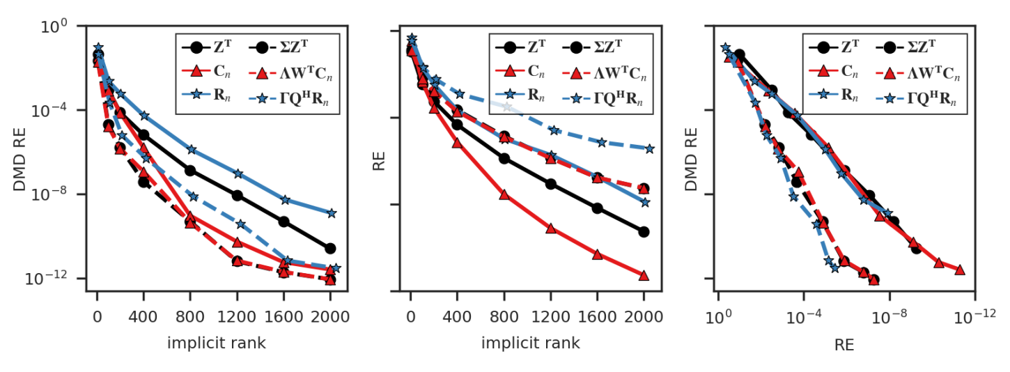
Figure 3: DMD experiment results. Left: variation in DMD relative error ($\|\bm{\mathcal{A}}_{\text{DMD}}{\star}_{{\scriptscriptstyle{\hskip-1.0pt\mathbf{M}}\hskip 1.0pt}}\bm{\mathcal{X}}-\bm{\mathcal{Y}}\|_{F}^{2}/\|tY\|_{F}^{2}$) in implicit target rank. Middle: Reconstruction error ($\|\bm{\mathcal{X}}-\bm{\mathcal{X}}_{(r)}\|_{F}^{2}/\|\bm{\mathcal{X}}\|_{F}^{2}$ where $\bm{\mathcal{X}}_{(r)}$ is the truncation of $\bm{\mathcal{X}}$ to implicit rank $r$ under ${\star}_{{\scriptscriptstyle{\hskip-1.0pt\mathbf{M}}\hskip 1.0pt}}$, i.e., zeroing all but the top-$r$ singular values) vs. implicit rank $r$. Right: DMD relative error obtained for varying implicit target rank $r$.

Then, Figure 4 shows how low-energy frequencies of the data-driven and DCT transforms can introduce spurious artifacts in the DMD reconstructions, which are mitigated when using the scaled versions of these transforms.

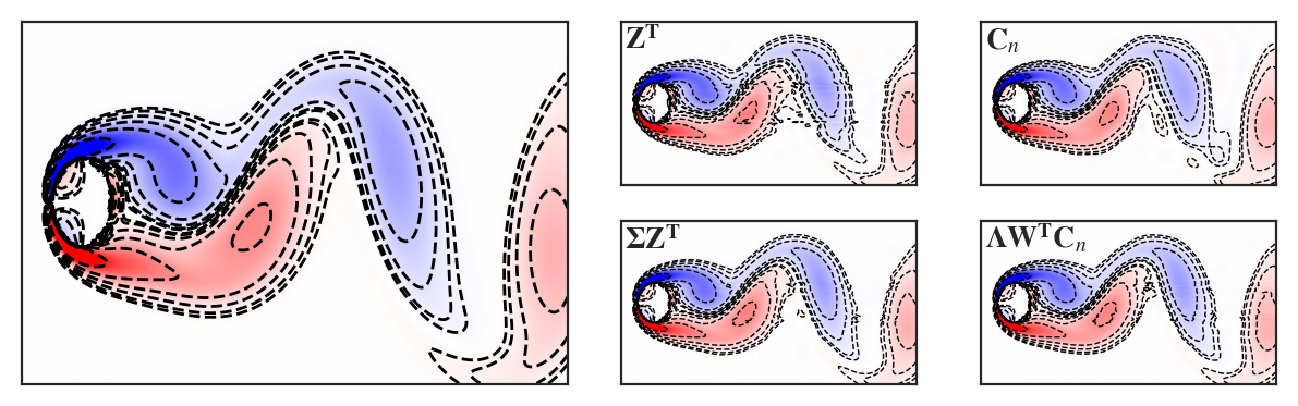
Figure 4: 2d state reconstruction for the last snapshot in $\bm{\mathcal{A}}_{\text{DMD}}{\star}_{{\scriptscriptstyle{\hskip-1.0pt\mathbf{M}}\hskip 1.0pt}}\bm{\mathcal{Y}}$, using the approximate $\bm{\mathcal{A}}_{\text{DMD}}$ obtained from truncating the tSVDM of $\bm{\mathcal{X}}$ to retain $\gamma=0.975$ of the energy, w.r.t the unscaled (top row) and scaled (bottom row) versions of the data-driven transform (middle column) and DCT (right column).

8 Conclusions

In this work, we have fully characterized the family of transforms that yield Eckart-Young optimal tSVDMII approximations. The notion of tubal length was key to this characterization, as it allowed us to express the approximation error in a simple form that is independent of the choice of transform. The definition of tubal length is itself an interesting contribution, as it generalizes matrix rank to the tubal-tensor setting in a way that is consistent with our expectations regarding the images and kernels of linear operators.

The practical implications of our theoretical results were discussed in the context of data analysis tasks that rely on low-rank tensor approximations. We show that non-uniformly scaled transforms are generally not beneficial for data compression tasks, but can be advantageous in applications where certain frequencies of the data are more relevant than others.

Appendix A Rings, Ideals, and Modules

A ring is a set $R$ equipped with two binary operations, addition $+$ and multiplication $\cdot$, such that $(R,+)$ is an Abelian group, multiplication is associative, distributive over addition from both sides, and there exists neutral elements $0_{R}\in R$ for addition and $1_{R}\in R$ for multiplication. A commutative ring is a ring where multiplication is commutative. For our purposes, all rings considered in this work are commutative and unital.

Definition A.1.

An ideal $I$ of a ring $R$ is a subset $I\subseteq R$ that is closed under addition, such that $r\cdot s\in I$ for all $r\in R$ and $s\in I$.

Let $R$ be a ring, an $R$-module is an Abelian group $(M,+)$ equipped with a scalar multiplication operation $\cdot:R{\times}M\to M$ that is distributive over addition in both $R$ and $M$, and associative with multiplication in $R$, i.e., for all $r_{1},r_{2}\in R$ and $m_{1},m_{2}\in M$ we have $(r_{1}+r_{2})\cdot m_{1}=r_{1}\cdot m_{1}+r_{2}\cdot m_{1}$, $r_{1}\cdot(m_{1}+m_{2})=r_{1}\cdot m_{1}+r_{1}\cdot m_{2}$, and $(r_{1}\cdot r_{2})\cdot m_{1}=r_{1}\cdot(r_{2}\cdot m_{1})$. It therefore holds that $1_{R}\cdot m=m$ and $0_{R}\cdot m=0_{M}$ for all $m\in M$. A submodule $N$ of an $R$-module $M$ is a subset $N\subseteq M$ that is closed under addition and scalar multiplication by elements of $R$.

The above definitions of ideals and modules are usually given in the context of general rings, where it is necessary to distinguish between left ideals/modules and right ideals/modules. However, since we only consider commutative rings in this work, the distinction is unnecessary, and we simply refer to ideals and modules.

Definition A.2.

Let $R$ be a ring, and let $M_{1},M_{2}$ be $R$-modules. A mapping $T:M_{1}\to M_{2}$ is called an $R$-module homomorphism if for all $s,r\in R$ and $m_{1},m_{2}\in M_{1}$ we have $T(r\cdot m_{1}+s\cdot m_{2})=r\cdot T(m_{1})+s\cdot T(m_{2})$. The set of all $R$-module homomorphisms from $M_{1}$ to $M_{2}$ is denoted by $\operatorname{Hom}_{R}(M_{1},M_{2})$.

A bijective module homomorphism is called an $R$-module isomorphism, and if such an isomorphism exists between $M_{1}$ and $M_{2}$, we say that $M_{1}$ and $M_{2}$ are isomorphic as $R$-modules, denoted by $M_{1}\cong M_{2}$.

Definition A.3 (Generating Set).

Let $R$ be a commutative ring, and $M$ be an $R$-module.

A subset $\Gamma\subseteq M$ is a generating set of $M$ if every element $m\in M$ can be expressed as a linear combination of elements of $\Gamma$, i.e., $m={\sum}_{j=1}^{J}r_{j}g_{j}$ for some $\{g_{j}\}_{j=1}^{J}\subseteq\Gamma$ and $\{r_{j}\}_{j=1}^{J}\subseteq r$.

Definition A.4 (Generated submodule).

Let $R$ be a commutative ring, and $M$ be an $R$-module. Let $S\subset M$ be a subset of $M$.

$$\langle S\rangle=\left\{{\sum}_{j\in J}r_{j}s_{j}|r_{j}\in R,s_{j}\in S,J<\infty\right\}\subseteq M$$

Note that $\langle S\rangle$ is a submodule of $M$, and is the smallest submodule of $M$ that contains $S$. Hence, $\langle S\rangle$ is defined as the submodule of $M$ generated by $S$.

Definition A.5 (Basis and Free-Modules).

Let $R$ be a ring, and $M$ be an $R$-module. A subset $S\subset M$ is a basis of $M$ if 1) $\langle S\rangle=M$ and 2) $S$ is minimal: ${\sum}_{j=1}^{J}r_{j}s_{j}=0_{M}$ for $s_{j}\in S$ and $r_{j}\in R$ if and only if $r_{j}=0_{R}$ for all $j=1,\dots,J$,

An $R$-module $M$ is free if it admits a basis.

The notion of free modules generalizes the notion of vector spaces over fields to modules over rings. Just as an $n$-dimensional vector space over $\mathbb{F}$ is isomorphic to $\mathbb{F}^{n}$, for an $R$-module $M$ with a basis $E$ we have $M\cong R^{(E)}={\bigoplus}_{e\in E}R$, i.e., the direct sum of copies of $R$ indexed by the elements of $E$. Yet, it is possible that a free module admits bases of different cardinalities, hence the notion of dimension is not well-defined for free modules in general.

Definition A.6 (Invariant Basis Number (IBN) and Ranks of Free Modules).

A ring $R$ has the Invariant Basis Number (IBN) if for every free $R$-module $M$ it holds that any two bases of $M$ have the same cardinality.

Suppose that $R$ has the IBN property, then, the cardinality of any basis of a free $R$-module $M$ is called the rank of $M$.

A fundamental result is that nonzero commutative rings have the IBN property.

Corollary A.7.

Let $R$ be a commutative ring, and $M$ be a finitely generated $R$-module.

Then $M$ is free if and only if there exists $N\in\mathbb{N}$ such that $M\cong R^{N}$.

Appendix B Cars experiment - Technical Workflow

After adding noise to the original video frames, we construct a data tensor $\bm{\mathcal{X}}\in\mathbb{R}^{256{\times}41{\times}455}$, and compute the consecutive difference tensor (in absolute value) $\bm{\mathcal{Y}}\in\mathbb{R}^{256{\times}40{\times}455}$, where $\bm{\mathcal{Y}}(:,i,:)=\bm{\mathcal{X}}(:,i+1,:)-\bm{\mathcal{X}}(:,i,:)$ for $i=1,\dots,40$ to highlight the moving objects in the video. To create a mask for the regions of interest (ROI) corresponding to moving vehicles, we apply spatial convolution to the values of $\bm{\mathcal{Y}}$ greater than its 90’th percentile using a $15{\times}15$ standard Gaussian kernel. The resulting mask is then filtered by removing once again all valued below the 90’th percentile.

In Figure 5, we present the process of generating the noisy video frames and mask for one of the frames in the sequence. You can observe that that due to the added noise, the moving vehicles are not easily distinguishable in the noisy frame. Furthermore, the noise also causes the masking of some background components, especially on regions outside the road, which have more composite textures.

Figure 5: The result of adding noise to the data and automatically masking moving objects

Figure 6: Showing the resulting tSVDMII approximations using the DCT (middle column, one component) and the scaled DCT (right, 220 components), for video frames 20 (top row) and 100 (bottom row) in the testing dataset.

Appendix C Beyond 3’rd Order Tensors

In consistence with the tubal precept, a $N+2$ order tensor $\bm{\mathcal{X}}\in\mathbb{R}^{m{\times}p{\times}n_{1}{\times}\cdots{\times}n_{N}}$ is an $m{\times}p$ matrix of $N$-way tubes $\bm{\mathcal{X}}(i,j,:,\ldots,:)\in\mathbb{R}^{n_{1}{\times}\cdots{\times}n_{N}}$.

Denote by $\Pi\coloneqq[n_{1}]{\times}\cdots{\times}[n_{N}]$ the multi-index set for $N$-way arrays in $\mathbb{R}^{n_{1}{\times}\cdots{\times}n_{N}}$ and consider any real tubal ring structure $\mathbb{R}_{\Pi}=(\mathbb{R}^{n_{1}{\times}\cdots{\times}n_{N}},+,\bullet)$, i.e., commutative, unital, Von Neumann regular ring that is also a real algebra.

Let $\iota\colon\mathbb{R}^{n_{1}{\times}\cdots{\times}n_{N}}\to\mathbb{R}^{|\Pi|}$ be any flattening, e.g., according to lexicographical ordering of multi-indices. Define a binary multiplication $\ast$ on $\mathbb{R}^{|\Pi|}$ as

$$\mathbf{a}\ast\mathbf{b}=\iota\left(\iota^{-1}(\mathbf{a})\bullet\iota^{-1}(\mathbf{b})\right),\quad\mathbf{a},\mathbf{b}\in\mathbb{R}^{|\Pi|}.$$

It is clear that $\iota$ is a ring (and $\mathbb{R}$-algebra) isomorphism between $\mathbb{R}_{|\Pi|}=(\mathbb{R}^{|\Pi|},+,\ast)$ and $\mathbb{R}_{\Pi}$, therefore $\mathbb{R}_{|\Pi|}$ is also a real tubal ring.

It follows from [AMDemystifying2025] that there exists an invertible linear transform $\mathbf{L}\in\mathbb{C}^{|\Pi|{\times}|\Pi|}$ such that

$$\mathbf{a}\ast\mathbf{b}=\mathbf{L}^{-1}\left((\mathbf{L}\mathbf{a})\odot(\mathbf{L}\mathbf{b})\right),\quad\mathbf{a},\mathbf{b}\in\mathbb{R}^{|\Pi|},$$

Furthermore, note that $\iota$ is also an isometry between inner-product spaces, i.e.,

$$\langle\bm{a},\bm{b}\rangle_{F}={\sum}_{\alpha\in\Pi}a_{\alpha}b_{\alpha}={\sum}_{j=1}^{|\Pi|}\iota(\bm{a})_{j}\iota(\bm{b})_{j}=\langle\iota(\bm{a}),\iota(\bm{b})\rangle_{F}$$

Therefore, by Theorem 5.1, setting $\mathbf{L}=\mathbf{D}\mathbf{Q}$ for any unitary $\mathbf{Q}\in\mathbb{C}^{|\Pi|{\times}|\Pi|}$ and diagonal $\mathbf{D}\in\mathbb{R}^{|\Pi|{\times}|\Pi|}$ such that Lemma 2.11 holds, we obtain a tubal ring structure $\mathbb{R}_{\Pi}$ that exhibits Eckart-Young optimality.