Informing Acquisition Functions via Foundation Models for Molecular Discovery

Abstract

Bayesian Optimization (BO) is a key methodology for accelerating molecular discovery by estimating the mapping from molecules to their properties while seeking the optimal candidate. Typically, BO iteratively updates a probabilistic surrogate model of this mapping and optimizes acquisition functions derived from the model to guide molecule selection. However, its performance is limited in low-data regimes with insufficient prior knowledge and vast candidate spaces. Large language models (LLMs) and chemistry foundation models offer rich priors to enhance BO, but high-dimensional features, costly in-context learning, and the computational burden of deep Bayesian surrogates hinder their full utilization. To address these challenges, we propose a likelihood-free BO method that bypasses explicit surrogate modeling and directly leverages priors from general LLMs and chemistry-specific foundation models to inform acquisition functions. Our method also learns a tree-structured partition of the molecular search space with local acquisition functions, enabling efficient candidate selection via Monte Carlo Tree Search. By further incorporating coarse-grained LLM-based clustering, it substantially improves scalability to large candidate sets by restricting acquisition function evaluations to clusters with statistically higher property values. We show through extensive experiments and ablations that the proposed method substantially improves scalability, robustness, and sample efficiency in LLM-guided BO for molecular discovery.

1 Introduction

Discovering molecules with desirable properties is crucial for drug design, materials science, and chemical engineering. Given the vast chemical space (restrepo_chemical_2022), exhaustive evaluation is infeasible, as density functional theory (DFT) simulations (parr_density_1989) are computationally expensive and experiments are laborious and time-consuming. Bayesian Optimization (BO, frazier_tutorial_2018; garnett_bayesian_2023) promises to minimize costly evaluations and accelerate discovery by using acquisition functions, expressed as the expected utility under a surrogate model (e.g., Gaussian Processes (GPs) and Bayesian Neural Networks (BNNs)) to guide the search toward promising candidates, balancing exploration of uncertain regions with exploitation of high observed-value regions.

However, the high cost of evaluations limits the number of initial points available to seed BO with informative Acquisition Function (AF) priors (typically $\sim$10 in previous studies (xie_bogrape_2025; kristiadi_sober_2024)), further constraining its performance. Recent approaches incorporate LLM priors into BNNs (kristiadi_sober_2024) with fixed features, parameter-efficient fine-tuning (PEFT; e.g., Low-Rank Adaptation (LoRA (hu_lora_2021))), or in-context learning (ICL; (ramos_bayesian_2023)), but they remain limited by scalability, cost, and computational challenges due to the vast discrete candidate space.

To address these challenges, we propose a principled likelihood-free BO method that avoids the costly Bayesian learning of a surrogate model, which (a) leverages rich prior knowledge from both general LLMs and specialized foundation models to inform AFs, and (b) partitions the molecular candidate space into a tree structure with local AF learned for each node, enabling efficient candidate selection via Monte Carlo Tree Search (MCTS) at each BO iteration given high-dimensional LLM features.

Our method directly models local AFs via density ratio estimation, which can be obtained by optimizing a binary classification objective at each tree node. These binary classifiers determine both the tree partitions and the corresponding local AFs. By meta-learning the shared LoRA weights and the initialization of the root node classifier, we enhance the stability of the binary classifiers, leading to more stable PEFT updates, even in low-data regimes. We further show that our proposed method, LLMAT (LLM-guided Acquisition Tree), visualized in Fig. 2, substantially improves the scalability, robustness, and sample efficiency of BO for molecular discovery.

Figure 1: General LLMs provide coarse property ranking of redox potentials rather than accurate numeric value for the three given molecules; responses are color-matched.

Finally, we observed that, although general LLMs are primarily trained on natural language and cannot predict precise numerical property values without in-context learning (ICL), they can capture coarse-grained information, such as whether a molecule’s property is relatively high or low. As shown in Fig. 1, while LLM-predicted redox potentials are not numerically accurate, the relative ordering of molecules is largely preserved. Building on this observation, we introduce an LLM-based clustering phase that queries a general LLM once to assign cluster labels to the entire candidate set. This cluster information is then used to improve scalability and BO performance by restricting AF evaluations to clusters with statistically higher property values.

To summarize, the main contributions of our paper are the following:

• We propose a likelihood-free BO method that leverages both general LLMs and specialized foundation models to inform AFs in a mathematically principled way. Our method also learns a tree-structured partition of the vast molecular search space and local AFs for the nodes with shared binary classifiers, enabling efficient candidate selection and local AF estimation via MCTS.

• To further improve the stability of partitioning and local AFs in the low-data regime, we introduce a meta-learning approach for training the shared binary classifiers, which enables more reliable and generalizable acquisition functions across partitions.

• We introduce an LLM-guided pre-clustering strategy along with a statistical cluster selection approach for BO, which estimates AF values only for candidates within selected clusters. This improves BO performance and reduces computational cost, particularly for PEFT, thereby mitigating the scalability challenges associated with vast candidate sets. Our approach provides a novel way to incorporate information from general LLMs into algorithm design with a reasonable API cost.

We evaluate our method on six real-world chemistry datasets and show that it outperforms baselines in most cases with improved scalability, benefiting from the prior knowledge in general LLMs, chemistry-specific foundation models, and the improved algorithm design.

2 Related Work

Due to space limitations, a more detailed discussion of related works is provided in Appendix B.

LLMs for Molecule Discovery. Recent studies have explored the potential of LLMs in a variety of chemistry-related tasks, including molecular property prediction (lu_unified_2022; christofidellis_unifying_2023; guo_what_2023; jablonka_14_2023), property-related molecule optimization (ramos_bayesian_2023; kristiadi_sober_2024), and molecular generation with desired properties (liu_conversational_2023; flam-shepherd_language_2023; wang_efficient_2024; jablonka_leveraging_2024). However, many of these LLM-based approaches (ramos_bayesian_2023; guo_what_2023) rely heavily on in-context learning (ICL) and prompt engineering. This dependency poses challenges for tasks involving strict numerical objectives, where LLMs often fall short in satisfying precise quantitative constraints or optimizing for specific target values (ai4science_impact_2023). To address this limitation, recent efforts have augmented LLMs with optimization frameworks such as Bayesian Optimization (BO) or Evolutionary Algorithms (EA). For example, kristiadi_sober_2024 integrate Laplace approximations with Bayesian neural networks for property prediction, while wang_efficient_2024 combine EA to generate and search molecules with desired property.

LLMs for Bayes Optimization over Molecules. General LLMs and chemistry foundation models capture rich priors from text and molecular datasets, offering the potential to guide BO in low-data regimes. Recent studies have explored this potential through various adaptations. For example, ramos_bayesian_2023 implemented BO via ICL by adaptively prompting general-purpose LLMs like GPT-4, which is effective but costly due to accumulated API queries and limited by prompt length. Alternatively, kristiadi_sober_2024 used LLMs for fixed-feature extraction and PEFT (hu_lora_2021; li_prefix-tuning_2021) in the BO loop, requiring expensive Laplace approximations of BNNs across the full candidate set and imposing high computational and memory demands. Moreover, relying on a single surrogate trained on limited data can be suboptimal, especially for high-dimensional LLM embeddings (wang_learning_2020). In contrast, our method directly leverages these priors to guide acquisition functions without costly surrogate learning and incorporates LLM-based clustering to restrict evaluations to promising regions, enabling scalable and data-efficient BO in large, high-dimensional molecular spaces.

3 Background

3.1 Bayesian Optimization

Bayesian Optimization (BO) aims to effectively maximize some unknown function $f:{\mathcal{X}}\rightarrow{\mathcal{Y}}$ over the candidate space ${\mathcal{X}}$, i.e., find $x^{*}=\arg\max_{x\in\mathcal{X}}f(x)$ , given a dataset $\mathbf{D}_{t}=\{x_{i},y_{i}\}_{i=1}^{t}$ of $t$ observations, where $x_{i}$ is a molecule, $y_{i}=f(x_{i})+\epsilon,\forall i\in[t]$ is a property value, and $\epsilon$ is noise conventionally assumed to be a Gaussian with $\epsilon\sim{\mathcal{N}}(0,\sigma^{2})$. Due to the intractability of $f$, a probabilistic surrogate model $\hat{f}$ learned from $\mathbf{D}_{t}$ is often used to approximate $f$ with consideration of epistemic uncertainty, reflected in the variance of the posterior $p(\hat{f}|\mathbf{D}_{t})$. Hence, for any unobserved data $(x,y)$, we have the predictive posterior $p(y|x,\mathbf{D}_{t})=\int p(y|\hat{f}(x))p(\hat{f}(x)|\mathbf{D}_{t})d\hat{f}(x)$.

Acquisition Function (AF) and Expected Utility. To address problems in the sequential decision-making setting, Bayesian Optimization (BO) methods typically select the next query $x_{t+1}$ by maximizing an acquisition function $\alpha:\mathcal{X}\to\mathbb{R}$, defined as:

$$\alpha(x;\mathbf{D}_{t},\tau):=\mathbb{E}_{y\sim p(y|x,\mathbf{D}_{t})}[u(y;\tau)],$$ (1)

where $x_{t+1}=\arg\max_{x\in{\mathcal{X}}}\alpha(x;\mathbf{D}_{t},\tau)$, $u(y;\tau)$ is a chosen utility function and $\tau$ is a threshold that measures the utility of $y$. The selection of $\tau$ controls the exploration-exploitation trade-off, and sometimes is set as $\tau=\max_{t}y_{t}$, the best observed value so far. Common choices of the utility function $u(y;\tau)$ satisfying Eq.(1) include: $u^{EI}(y;\tau)=\max(y-\tau,0)$ for Expected Improvement (EI, mockus_toward_1978) that measures how much $y$ exceeds the threshold $\tau$; $u^{PI}(y;\tau)={\mathbf{1}}(y-\tau>0)$, indicating whether $y$ exceeds $\tau$ for Probability of Improvement (PI, kushner_new_1964); Many other AFs can be expressed as the expected utility with a more complex utility function, such as Upper Confidence Bound (UCB, srinivas_gaussian_2009), Entropy Search (ES, hennig_entropy_2012), Knowledge Gradient (KG, frazier_knowledge-gradient_2008), Thompson Sampling (TS, thompson_likelihood_1933).

Direct Estimation of Acquisition Functions. Typical BO instantiations can be characterized as indirect: they first approximate the predictive posterior $p(y\mid x,\mathbf{D}_{t})$ via a surrogate model based on Gaussian Processes (GPs) or Bayesian Neural Networks (BNNs), and then compute the acquisition functions via Eq. (1) for a given utility function. We provide an introduction to this in Appendix A.1. However, these methods often face scalability issues due to the high computational cost when combining large, deep models, which limits their flexibility. Our proposed method on the other hand directly models AFs, forgoing the need for surrogate model. Let $l(x)=p(x|y\leq\tau,\mathbf{D}_{t})$ and $g(x)=p(x|y>\tau,\mathbf{D}_{t})$ be two densities that respectively characterize the data distribution on non-promising and promising region of candidate space. Instead of explicitly modeling the predictive posterior $p(y|x,\mathbf{D}_{t})$, bergstra_algorithms_2011 and tiao_bore_2021 directly model the acquisition function as the following $\gamma$-relative density ratio:

$$r_{\gamma}(x):=\frac{g(x)}{\gamma g(x)+(1-\gamma)l(x)}=h_{\gamma}(r_{0}(x))\,,$$ (2)

where $h_{\gamma}:u\rightarrow(\gamma+u^{-1}(1-\gamma))^{-1},u>0$ is strictly non-decreasing, $r_{0}(x)=\frac{g(x)}{l(x)}$ is the ordinary density ratio, and $\gamma=p(y>\tau|\mathbf{D}_{t})$ indicates $\tau$ is set as the $\gamma$-th quantile of all observed $y$. This density ratio has been proven by song_general_2022 to be equivalent to PI . Tree Parzen Estimator (TPE, (bergstra_algorithms_2011)) estimates the density ratio $r_{0}(x)$ by separately estimating $\ell(x)$ and $g(x)$ with tree variant of Kernel Density Estimation (KDE). BORE (tiao_bore_2021) avoids such indirect estimation by formulating the problem as a binary classification and showing the classifier $\pi_{\theta}(x)\approx p(c=1|x,\mathbf{D}_{t})=\gamma r_{\gamma}(x)$, where $c={\mathbf{1}}(y>\tau)$ is the class label and $p(c=1|\mathbf{D}_{t})=p(y>\tau|\mathbf{D}_{t})=\gamma$. Likelihood-free Bayes Optimization (LFBO, song_general_2022) adopts variational $\phi-$divergence estimation to directly estimate general expected utility AFs for complex $p(y|x,\mathbf{D}_{t})$ and $u(y;\tau)$, not limited to PI. Then, the likelihood-free AF is defined as:

$$\alpha(x;\mathbf{D}_{t},\tau):=\pi_{\theta^{*}}(x)/(1-\pi_{\theta^{*}}(x))\,,$$ (3)

where $\pi_{\theta}(x):=p_{\theta}(c=1|x,\mathbf{D}_{t})$, $\theta^{*}=\arg\min_{\theta}{\mathcal{L}}^{\tau}_{\mathbf{D}_{t}}(\theta)$,

$${\mathcal{L}}^{\tau}_{\mathbf{D}_{t}}(\theta):=\mathbb{E}_{(x,y)\sim\mathbf{D}_{t}}[-u(y;\tau)\log\pi_{\theta}(x)-\log(1-\pi_{\theta}(x))]\,.$$

3.2 BO for Molecular Discovery

In molecular discovery, the goal is to identify a novel molecule $x\in{\mathcal{X}}$ with desirable properties $y\in{\mathcal{Y}}\subseteq{\mathbb{R}}$, often requiring exploration of a vast and discrete search space ${\mathcal{X}}$ (estimated to contain over $10^{100}$ unique molecules). Exhaustively verifying property values is infeasible and costly, e.g., when relying on Density Functional Theory (DFT). In practice, experimental discovery restricts the search to a smaller candidate subset $\Omega\subset{\mathcal{X}}$. At each round $t+1$, given prior observations $\mathbf{D}_{t}=\{x_{i},y_{i}\}_{i=n+1}^{n+t}\cup\mathbf{D}_{0}$ with $n$ initial points $\mathbf{D}_{0}=\{x_{j},y_{j}\}_{j=1}^{n}$, a new candidate $x_{t+1}$ is selected from $\Omega\setminus\mathbf{D}_{t}:=\{x_{i}\in\Omega\mid x_{i}\notin\mathrm{supp}_{X}(\mathbf{D}_{t})\}$ for evaluation, with the aim of finding the optimal molecule $x^{*}$ in as few rounds as possible. This naturally fits the sequential BO framework.

To input molecules into machine learning models, common representations (griffiths_gauche_nodate; janakarajan_language_2024) include: (1) text-based formats such as SMILES (weininger_smiles_1988), SELFIES (krenn_self-referencing_2020), and IUPAC names; (2) feature-based fingerprints such as Morgan (morgan_generation_1965) and ECFPs (rogers_extended-connectivity_2010); and (3) graph-based encodings (duvenaud_convolutional_2015). In this work, we focus on text-based representations, which can be directly generated by modern NLP models, including general-purpose LLMs, transformer-based chemical foundation models, and domain-specific LLMs specialized for chemical data.

4 Methodology

As discussed previously, the early rounds of BO with limited observations, the high dimensionality of molecular features, and the vast discrete candidate space pose major challenges for efficient discovery. We address these challenges by leveraging LLMs to achieve: (1) Refined AF optimization. Local acquisition functions are learned on top of LLM/foundation model feature extractors while building the tree partition, combined with meta-learning of the root node initialization to mitigate overfitting for each sub-node. The next candidate is selected by comparing AF values within a small set of molecules in the most promising leaf node. (2) Improved computational efficiency. Evaluating AFs across the full candidate space is costly, especially with PEFT, so we employ LLM-based clustering and statistical testing to prune the search space before AF estimation. We refer to our method as LLM-guided Acquisition Tree (LLMAT), which integrates LLM-based clustering, foundation model representations, and tree-structured acquisition function learning for efficient molecular discovery. An overview is shown in Fig. 2.

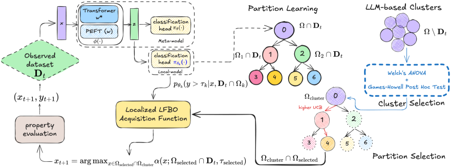
Figure 2: Overview of LLMAT: Binary classifiers on the LLM features recursively partition the candidate space to a tree structure and local AFs are learned from observations in each partition $\Omega_{k}\cap\mathbf{D}_{t}$. Promising partition $\Omega_{\text{selected}}$ is selected via UCB. Unseen candidates are clustered via LLM prompts, and promising clusters $\Omega_{\text{cluster}}$ are selected via statistical tests. Within $\Omega_{\text{cluster}}\cap\Omega_{\text{selected}}$, the property of the candidate with the highest local AF value is evaluated and added to the dataset.

4.1 Meta-Learning of Candidate Partitions and local Acquisition Functions

In this section, we introduce a meta-learning framework that trains shared binary classifiers for candidate partitioning and local AFs approximation when building the tree partition.

Algorithm 1 Meta-learning Tree Partitions and local AFs

1: Input: Observed dataset $\mathbf{D}_{t}$, quantile $\gamma$, candidate set $\Omega$, tree depth $L$, classification head $\theta$, PEFT parameters $w$, learning rate $\eta$, SGD steps $K$, finetuning flag $\mathbb{F}$, minimal leaf sample size $m$.

2: Nodes ${\mathcal{N}}=\{\}$;

3: $\Omega_{0}=\Omega,\mathbf{D}_{t}\cap\Omega_{0}=\mathbf{D}_{t},\mathbf{D}_{t}\cap\Omega_{k}=\emptyset,\forall k>0$;

4: for $k=0$ to $2^{L+1}-2$ do

5:  if $|\Omega_{k}\cap\mathbf{D}_{t}|<m$ or $\Omega_{k}$ not splitable then

6:   continue;

7:  end if

8:  $\tau_{k}=\Phi_{k}^{-1}(\gamma)$; Fix $w$, update $\theta_{k}=\text{SGD}({\mathcal{L}}^{\tau_{k}}_{\mathbf{D}_{t}\cap\Omega_{k}}(\theta,w),K)$;

9:  $\theta\leftarrow\theta+\eta(\theta_{k}-\theta)$, ${\mathcal{N}}\leftarrow{\mathcal{N}}\cup\{k\}$;

10:  for $(x,y)$ in $\mathbf{D}_{t}\cap\Omega_{k}$ do

11:   if $\pi_{\theta_{k}}(x)>0.5$ then

12:    $\mathbf{D}_{t}\cap\Omega_{2k+1}\leftarrow(\mathbf{D}_{t}\cap\Omega_{2k+1})\cup\{(x,y)\}$;

13:   else

14:    $\mathbf{D}_{t}\cap\Omega_{2k+2}\leftarrow(\mathbf{D}_{t}\cap\Omega_{2k+2})\cup\{(x,y)\}$;

15:   end if

16:  end for

17: end for

18: if $\mathbb{F}$ then

19:  Fix $\theta$, update $w=\text{PEFT}(\frac{1}{|{\mathcal{N}}|}\sum_{k\in{\mathcal{N}}}{\mathcal{L}}^{\tau_{k}}_{\mathbf{D}_{t}\cap\Omega_{k}}(\theta,w))$;

20: end if

21: Output: $\pi_{\theta_{k}}(x),\alpha(x;\Omega_{k}\cap\mathbf{D}_{t},\tau_{k}),\forall k\in{\mathcal{N}}$;

Recursive Candidate Space Partitioning. At any iteration $t$, we have the currently observed dataset $\mathbf{D}_{t}=\{x_{i},y_{i}\}_{i=1}^{n+t}$ defined in Sec. 3.1. As shown in Fig. 2, we use Monte Carlo Tree Search (MCTS) to hierarchically partition the candidate set $\Omega$, where each node in the tree corresponds to a subset of $\Omega$. The tree construction begins at the root node (node 0) with $\Omega_{0}=\Omega$ being the entire candidate space.

Each node $\Omega_{k}$ is recursively bifurcated into two subsets using a binary classifier $\pi_{\theta_{k}}$. Let $\Omega_{2k+1}:=\{x\in\Omega_{k}\mid\pi_{\theta_{k}}(x)>0.5\}$ and $\Omega_{2k+2}:=\{x\in\Omega_{k}\mid\pi_{\theta_{k}}(x)\leq 0.5\}$ be the left and right children respectively, representing the more promising (i.e., more likely to contain high-property candidates) and less promising regions. The tree expansion continues until a predefined maximum depth $L$ or the least number of samples in each node is reached, yielding a total maximum of $2^{L+1}-1$ nodes. To train the binary classifier at each node $\Omega_{k}$, we use the subset of observed samples within that node, i.e., $\mathbf{D}_{t}\cap\Omega_{k}:=\{(x_{i},y_{i})\in\mathbf{D}_{t}\mid x_{i}\in\Omega_{k}\}$, where their class labels can be obtained by directly thresholding $y$ as we described in the following. For unobserved samples in $\Omega_{k}$, the learned classifier $\pi_{\theta_{k}}$ assigns them to the left or right child. When estimating the AFs, rather than classifying all samples across the whole tree, we only route the search from the root to the most promising leaf, using classifiers at each node along that path.

Algorithm 2 Partition Selection for Refined and Reduced AFs

1: Input: Dataset $\mathbf{D}_{t}$, tree depth $L$, candidates in selected clusters $\Omega_{\text{cluster}}$, classifier $\theta$, learning rate $\eta$, SGD steps $K$, quantile $\gamma$, UCB hyper-parameter $\lambda$, time budget $T$, all nodes ${\mathcal{N}}$.

2: for $t=0$ to $T$ do

3:  Run Algo. 1;

4:  #Select the search tree path.

5:  Set $k=0$, $\tau_{k}=\Phi_{k}^{-1}(\gamma)$;

6:  Path ${\mathcal{P}}\leftarrow[]$;

7:  while $k\in{\mathcal{N}}$ do

8:   ${\mathcal{P}}\leftarrow{\mathcal{P}}+[k]$;

9:   Compute partition score for $2k+1$ and $2k+2$;

10:   $k=\arg\max_{j\in\{2k+1,2k+2\}}{\mathcal{S}}_{j}$;

11:  end while

12:  #Backtrack and select local AF up the path.

13:  ${\mathcal{P}}\leftarrow\text{Reverse}({\mathcal{P}})$;

14:  selected = 0;

15:  for each $k$ in ${\mathcal{P}}$ do

16:   if $|\Omega_{k}\cap\Omega_{\text{cluster}}|=0$ then

17:    continue;

18:   else

19:    selected = k;

20:    break;

21:   end if

22:  end for

23:  Sample $x_{t+1}=\operatorname*{arg\,max}\limits_{x\in\Omega_{\text{selected}}\cap\Omega_{\text{cluster}}}\alpha(x;\Omega_{\text{selected}}\cap\mathbf{D}_{t},\tau_{\text{selected}})$;

24:  Evaluate $y_{t+1}=f(x_{t+1})$;

25:  Update $\mathbf{D}_{t+1}\leftarrow\mathbf{D}_{t}\cup\{(x_{t+1},y_{t+1})\}$;

26: end for

LFBO Classifier Shared for Bifurcating. In LFBO, the AF at each iteration $t$ is estimated directly by learning a (weighted) binary classifier $\pi_{\theta}(x)=p_{\theta}(y>\tau|x,\mathbf{D}_{t})$, instead of training surrogate models for typical BO algorithms. This classifier can be reused as a natural choice for the aforementioned candidate space partitioning during the construction of the tree. At each node $k$, we set $\tau_{k}=\Phi_{k}^{-1}(\gamma)$ under the same $\gamma$, where $\gamma=\Phi_{k}(\tau_{k}):=p(y>\tau_{k}|\mathbf{D}_{t}\cap\Omega_{k})$. Then, the corresponding binary classifier is $\pi_{\theta_{k}}(x)=p_{\theta_{k}}(c=1|x,\mathbf{D}_{t}\cap\Omega_{k})$ with $c={\mathbf{1}}(y>\tau_{k})$, where the binary labels $c$ for training the classifier are assigned by thresholding the property value $y$ for all training samples in node $k$ instead of using the clustering approach in wang_learning_2020.

Meta-learning Shared Binary Classifiers.
Using a shared classification head connected after the transformer feature extractor, we propose a meta-learning approach that works for both fixed features and parameter efficient fine-tuning (PEFT). Since the tree is built recursively, we use the sequential version of Reptile (nichol_reptile_2018), meta-training the classification head. For a maximal $L$-depth Tree, we store one meta-model $\theta$ and $|{\mathcal{N}}|$ local models $\theta_{k},\forall k\in{\mathcal{N}}$. The detailed algorithm for learning the partitions and AFs at each iteration is presented in Algo. 1

4.2 Candidate Selection on Promising Subsets

With the built tree partition and learned local AFs, now we can perform refined AF estimation via partition selection and cluster selection to identify the most promising candidate in an efficient way.

Partition Selection. Given the aforementioned partition rule, a greedy strategy that always selects the left node would exploit the most promising leaf but risks overfitting to suboptimal partitions without sufficient exploration. To balance exploration and exploitation, we select partitions using some score metrics. For example, as in wang_learning_2020, let $n_{k}=|\mathbf{D}_{t}\cap\Omega_{k}|$ denote the visit count for each node $k$, and let the node value $v_{k}=\frac{1}{n_{k}}\sum_{i=1}^{n_{k}}y_{i}$ be the average property value of observed samples at node $k$. Then, the Upper Confidence Bound for Trees(UCT) score for a node $k\in{\mathcal{N}}$ is then defined as: ${\mathcal{S}}^{\text{UCT}}_{k}:=v_{k}+2\lambda\sqrt{2\log(n_{p})/n_{k}}$, where $p=\lceil\frac{k}{2}\rceil-1$ and $n_{p}$ is the number of visits at the parent node of $k$-th node and $\lambda$ is a hyper-parameter that controls the exploration-exploitation trade-off. Another possible choice is ${\mathcal{S}}^{\text{Var}}_{k}:=v_{k}+2\lambda\sqrt{\text{var}_{k}}$, where $\text{var}_{k}=\frac{1}{n_{k}}\sum_{i=1}^{n_{k}}(y_{i}-v_{k})^{2}$. When $\lambda=0$, both recover the greedy policy. Finally, we select the child node with the highest score from the root to a leaf. If no candidates reach a leaf node, we use a backtracking approach that selects the parent node instead. The selected partition is denoted as $\Omega_{selected}$, as illustrated in Algo. 2.

Clustering for Efficient Estimation of AFs. To reduce the high GPU memory and computation cost of calculating AFs for all candidates at each BO round, we propose a clustering-based approach. Molecular feature representations are precomputed once and grouped into clusters. Candidates within the selected clusters then undergo the partition selection process, and the optimal candidate is determined by comparing AFs only for $\Omega_{\text{cluster}}\cap\Omega_{selected}$.

(1) Cluster Selection via Statistical Test. To identify promising clusters for reduced AF estimation, we propose a statistical filtering approach based on observed data $\mathbf{D}_{t}$. Specifically, Welch’s ANOVA (Appendix A.3) that is robust to heterogeneous variances is first tested. For a given p-value $p$, if significant differences are detected in average property values across clusters, the Games-Howell post-hoc test (Appendix A.4) is applied to exclude outlier clusters using the same $p$. To support this, the BO initialization $\mathbf{D}_{0}$ is constructed by uniformly sampling candidates from each cluster.

(2) LLMs for Property-Related Clustering. Unsupervised clustering methods (e.g., k-means) do not guarantee grouping by property values, limiting the effectiveness of our cluster selection strategy. In contrast, general-purpose LLMs (e.g., ChatGPT) can provide property-aware clustering by classifying molecules into high, medium, or low property groups via tailored prompts, as what we used in Appendix C. This leverages the chemical knowledge embedded in their training corpora, yielding clusters aligned with property values. As shown in the experiments, it can enhance BO performance at a cost that is orders of magnitude lower than the ICL-based approaches reported in kristiadi_sober_2024, thereby providing a highly cost-effective way to exploit general LLMs.

5 Experiments

In this section, we experimentally validate the proposed algorithm across multiple datasets and ablation scenarios, demonstrating its ability to accelerate molecular discovery through superior BO performance and increased computational efficiency. All results are averaged over 15 independent runs with different random seeds. Additional details and results are provided in Appendix D and E.

5.1 Setting

Datasets. We employ the well-known multi-modal Levy function (levy_topics_2006) to generate a synthetic set to demonstrate the effectiveness of the proposed method in achieving more refined AF estimation within localized sub-regions. For molecular data, following kristiadi_sober_2024, we initialize BO with $n=10$ points and and evaluate our models on six benchmark datasets that capture realistic molecular design challenges across diverse domains: (1) minimizing redox potential for redoxmers (1,407 molecules), (2) minimizing solvation energy for flow battery electrolytes (1,407 molecules) (agarwal_discovery_2021), (3) minimizing docking scores of kinase inhibitors (10,449 molecules) for drug discovery (graff_accelerating_2021), (4) maximizing fluorescence oscillator strength for laser materials (10,000 molecules) (strieth-kalthoff_delocalized_2024), (5) maximizing power conversion efficiency (PCE) in photovoltaic materials (10,000 molecules) (lopez_harvard_2016), and (6) maximizing $\pi$–$\pi^{*}$ transition wavelengths for organic photoswitches (392 molecules) (griffiths_data-driven_2022). Together, these tasks cover a broad spectrum of molecular properties, providing a comprehensive testbed for molecular discovery. For each dataset, the physics-based simulators released by the original authors are used as the ground-truth oracles.

Fixed Features and Foundation Models. To assess whether the findings of kristiadi_sober_2024 that LLMs benefit molecular BO only when trained on domain specific data hold for our algorithm, we benchmark LLMAT against several baselines on using different features: (i) Morgan fingerprints (morgan_generation_1965) as a chemistry specific algorithmic representation, (ii) chemistry foundation models including T5-Chem (christofidellis_unifying_2023) and MolFormer (ross_large-scale_2022), and (iii) general LLMs such as T5 (raffel_exploring_2023), GPT-2 (radford_language_2019), and Llama-2-7b (touvron_llama_2023). Our comparison includes two settings: (1) Bayesian optimization using fixed feature representations extracted from these models, and (2) Parameter-Efficient Fine-Tuning (PEFT) of the above chemistry foundation models.

Evaluation Metrics. We report the trajectory of the best observed property value over time and use the GAP metric defined in jiang_binoculars_2020: $\text{GAP}_{t}:=\frac{y_{t}^{*}-y_{0}}{y^{*}-y_{0}},$ which normalizes the progression of the optimal value, where $y^{*}$ is the global optimum, $y_{0}$ is the initial optimum, and $y_{t}^{*}$ is the best value observed up to iteration $t$. However, in molecular discovery, identifying a single optimal molecule is often not the only goal. In practice, it is equally important to discover a set of high-performing candidates that scientists can further evaluate, balance against multiple criteria, or analyze for structure–property relationships. To capture this objective, we additionally report the average regret: $\text{Regret}_{t}:=\frac{1}{t}\sum_{i=1}^{t}\big(y^{*}-y_{i}\big),$ which reflects the overall quality of the molecules discovered so far. When aggregating results across datasets, we normalize the average regrets for comparability.

5.2 Performance Analysis

Effectiveness of Localized Search on Synthetic Data. Beyond LLM adaptation and its application to molecular discovery, our method contributes a novel discrete BO algorithm: we introduce shared binary classifiers that jointly serve both tree partitioning and localized AF approximation. To illustrate this benefit, we sample 1,000 examples from the Levy-1D function and observe that the proposed algorithm yields a more refined AF estimate at the selected leaf node than at the root node used by vanilla LFBO (song_general_2022). As shown in Fig. 3, the leaf node exhibits a narrower and more accurate confidence region around the true optimum, and the refinement becomes more pronounced over BO iterations as additional observations accumulate.

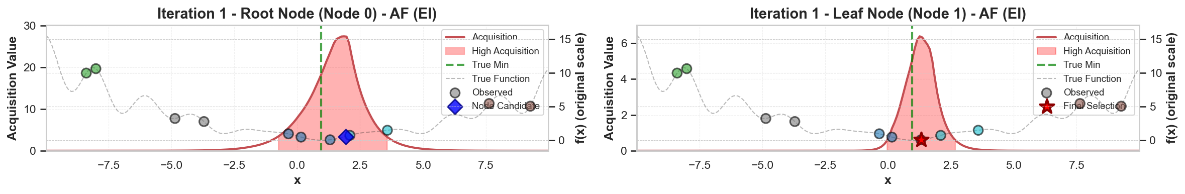
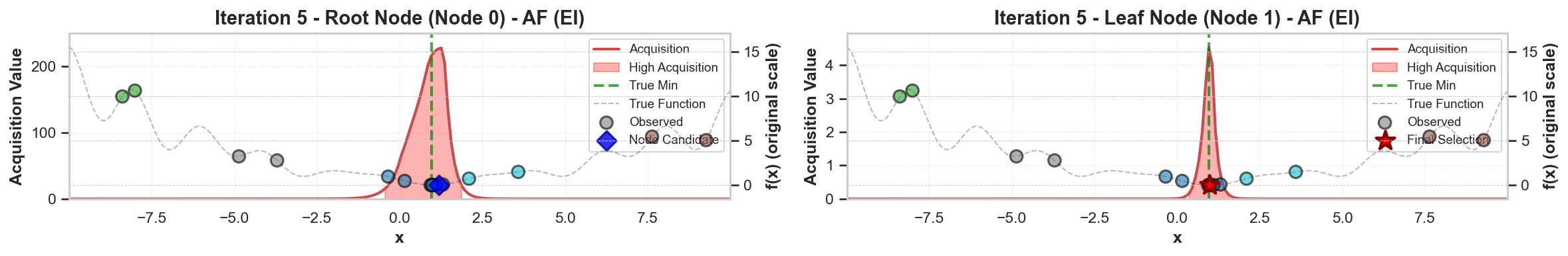
Figure 3: Leaf-node AFs offer more fine-grained candidate suggestions for Levy-1D optimization.

Superior Performance across Fixed-Features and Fine-Tuned Models on Molecular Data.  In the left panel of Fig. 4, we show that the proposed LLMAT algorithm outperforms standard discrete BO baselines when applied to fixed features extracted from the aforementioned models: Gaussian Processes (GP), the Laplace approximation (LAPLACE) (kristiadi_sober_2024), Likelihood-Free BO (LFBO), BORE (tiao_bore_2021), and random search (RANDOM), as measured by the average GAP metric across all datasets and models. The middle and right plot of Fig. 4 further compares LLMAT against LAPLACE across all datasets to assess iterative PEFT effectiveness with T5-Chem and Molformer backbones. While iterative PEFT enhances BO performance for both approaches, LAPLACE with PEFT still falls short of the performance achieved by our algorithm without PEFT. The radar chart in the left of Fig. 7 measures fine-tuning improvements over fixed features across six metrics demonstrates that our method achieves: (1) faster convergence in early BO rounds, (2) superior final performance, and (3) greater stability across different foundation models. The PEFT improvements are more substantial for Molformer than T5-Chem, reflecting T5-Chem’s larger scale and richer domain-specific knowledge.

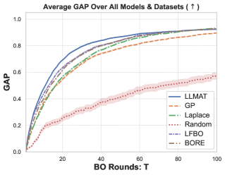
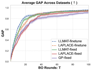
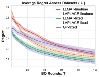
Figure 4: Left: Comparison over baselines on fixed features across all models and datasets. Middle& Right: Average GAP and regret (definition in 5.1) across datasets for fine-tuned (PEFT on $w$) and fixed ($w^{*}$) T5-chem model.

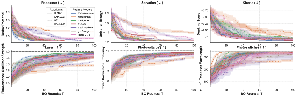
Figure 11: BO process for different datasets on features extracted from various foundation models.

Better Exploitation of Model Priors on Fixed Features.  In Fig. 5, we compare LLMAT (with maximal tree depth $L=1$ of $3$ nodes) against GP, LAPLACE, and RANDOM, using various fixed features mentioned before. We only plot the feature that achieved the best performance for each algorithm; the full plot is deferred to Fig. 11. Fig. 5 shows that LLMAT achieves superior performance compared to all baselines on most datasets, with slightly lower performance than LAPLACE on the Laser dataset. Other baselines exhibit substantial performance drops on several datasets while LLMAT remains consistent. LLMAT, LAPLACE, and GP achieve their best performance on the same feature models for the Redox-mer, Kinase, and Laser datasets (T5-Chem, T5, and MolFormer, respectively.). However, the best feature models differ for other datasets. The strong performance of LLMAT with T5, GPT-2-large, llama2-7b, and Morgan fingerprints suggests that general-purpose LLMs can still provide valuable information. This contrasts with kristiadi_sober_2024, who argue that LLMs are useful for BO over molecules only when pretrained or finetuned on domain-specific data, highlighting the importance of algorithmic design to fully exploit prior in different models.

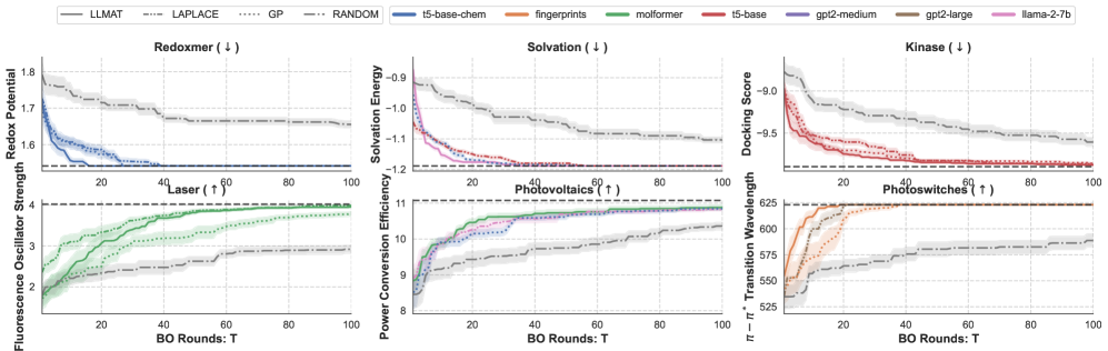
Figure 5: BO with fixed features (best-performing feature per algorithm shown). LLMAT achieves best overall performance, attaining top results on Solvation, Kinase, and Photoswitches using features from non-domain-specific models. The black dashed line marks the true optimum for each dataset.

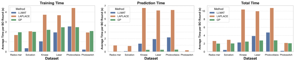
Figure 21: Computation time of different algorithms with fixed T5-Chem features across datasets.

Improved Computational Efficiency.  We also report training time, AF prediction time, and overall runtime per BO round using T5-chem features in Fig. 21. Our method achieves the shortest training time across all datasets. While prediction time increases slightly for the largest datasets (Kinase, Laser, Photovoltaics), this overhead is offset by GP’s poor performance on them. By contrast, LAPLACE incurs the highest overall cost, especially for predicting AFs during PEFT, making it the least efficient.

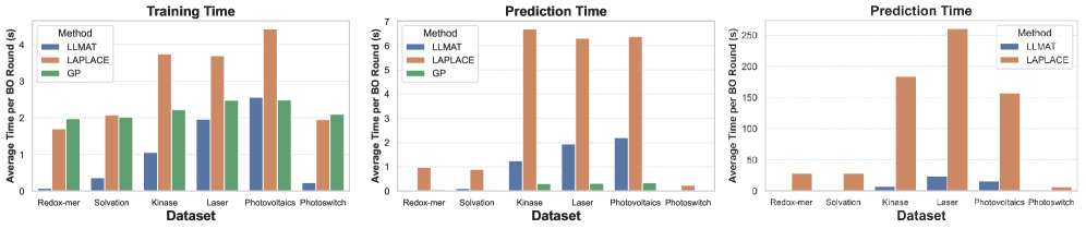
Figure 6: Left & Middle: Training and Prediction time of different methods on fixed ($w^{*}$) T5-Chem features. Right: Prediction time of LLMAT and LAPLACE for finetuning T5-chem (PEFT on $w$).

5.3 Ablation Studies

To understand the behavior of LLMAT, evaluate its module-wise effectiveness, and assess its robustness to noise, we conduct comprehensive ablation studies in this section.

Tree Depth Ablation: Improved Performance via Refined AFs.  The middle and right plots in Fig. 7 present an ablation on tree depths for LLMAT, which further strengthen the impact of refined acquisition functions (AFs). It shows that using only LFBO ($L=0$) performs significantly worse compared to deeper tree depths. With PEFT, performance peaks at depth $2$, demonstrating the benefit of deeper partitions, while with fixed features, performance is highest at depth $1$ and declines beyond due to over-partitioning.

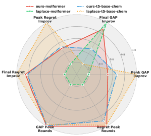
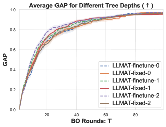
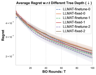
Figure 7: Left: Effectiveness of PEFT on T5-Chem and Molformer. Middle&Right: Tree-depth ablation on fixed and Finetuned Molformer across datasets, showing the importance of tree partition.

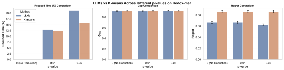
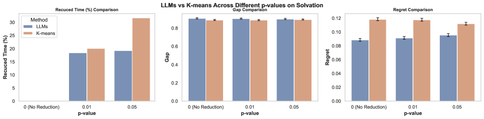
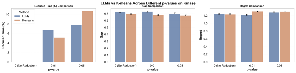
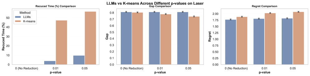
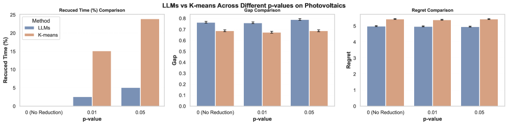
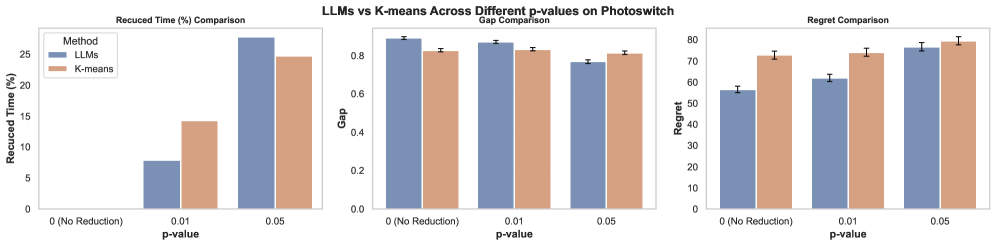
Figure 32: Prediction time reduction percentage, AUC of GAPs, and Regrets across all the datasets for different clustering approach and p-values.

Cluster Selection Ablation: LLMs Provide More Property-Relevant Information.  We compare LLM-based clustering with K-means on feature representations across different p-values, which determine the removal of clusters with significantly poorer property values. Fig. 8 shows that LLM-based clustering achieves better average GAP and regret at p-value = 0, highlighting its superior property-awareness for BO initialization. Increasing p-values filters more clusters during AF estimation, reducing prediction time by 10–25%. While LLM-based clustering removes fewer clusters than K-means at the same p-values, its performance remains stable at 0.01 and degrades only modestly at 0.05. In contrast, K-means is more prone to removing informative clusters, causing larger performance drops. Degradation does not always follow the p-value, as it depends on the property-cluster correlation. Fig. 32 shows LLM clustering removing irrelevant clusters on Redox-mer dataset, reducing computation and improving BO performance at the same time.

Figure 8: Average reduced prediction time percentage, average GAP, and average regret across six datasets for LLM-base clustering and K-means clustering w.r.t different p-values.

Ablation Study for Different Algorithmic Modules.  To provide a clearer understanding of the contribution of each algorithmic component in LLMAT, we conduct a detailed ablation study by selectively removing or adding modules and evaluating their impact on overall performance, as shown in the left plot of Fig. 9. The results indicate that both MCTS and meta-learning substantially enhance performance. LLM-based clustering offers a slight improvement, while K-means has a negligible effect. This is expected, as the clustering methods are primarily designed to reduce computational cost rather than directly boost optimization performance.

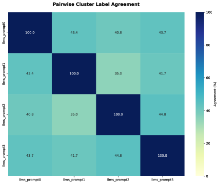
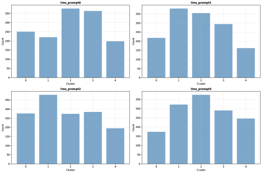
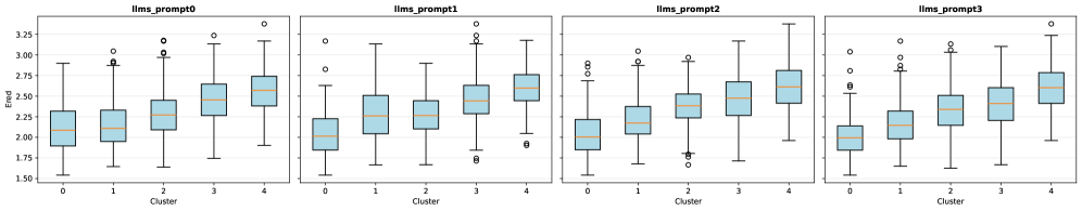
Figure 10: Prompt variation’s effect on cluster labels.

Sensitivity of Clustering prompts.  To evaluate LLMAT’s stability with respect to clustering prompts, we generated four similar prompts and compared their cluster labels agreements and cluster distributions in Fig. 10 in the Appendix. The right subplots of Fig. 9 show that the BO performance, measured by the GAP metric, remains largely consistent. This stability can be attributed to the statistical test used during cluster selection, which incorporates observed data to enhance robustness.

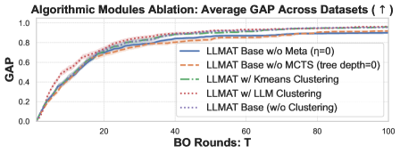
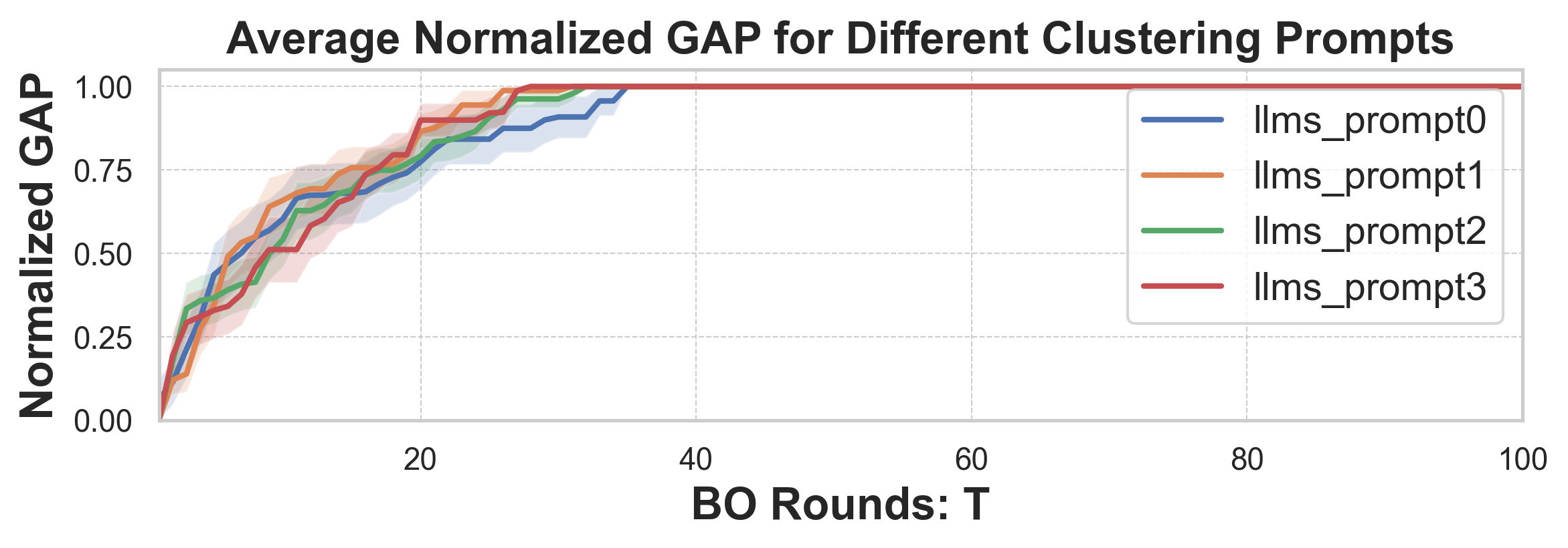
Figure 9: Left: Average GAP across six datasets illustrating the impact of individual algorithmic module ablations. Right: LLM Clustering Prompt Sensitivity in LLMAT on Redox-mer Data.

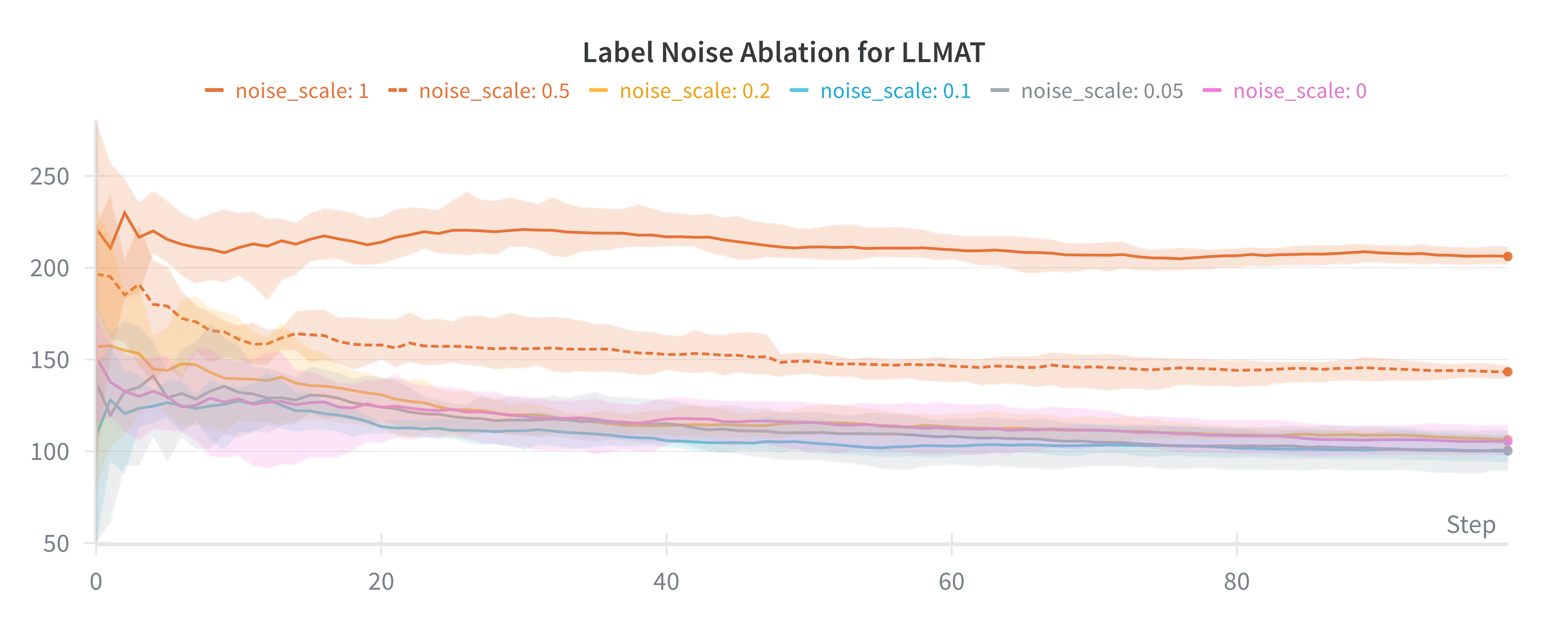
Figure 38: Illustration of Labal Noise’s affects on the average regret of LLMAT.

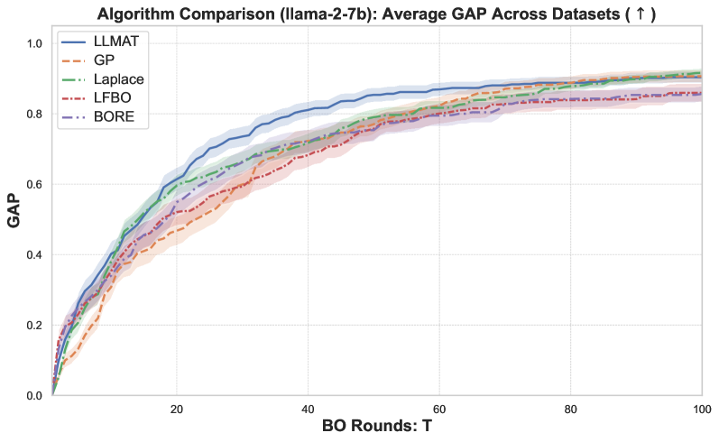
Figure 40: Illustration Performance Comparison of Various Algorithms on Llama2-7b across All Datasets.

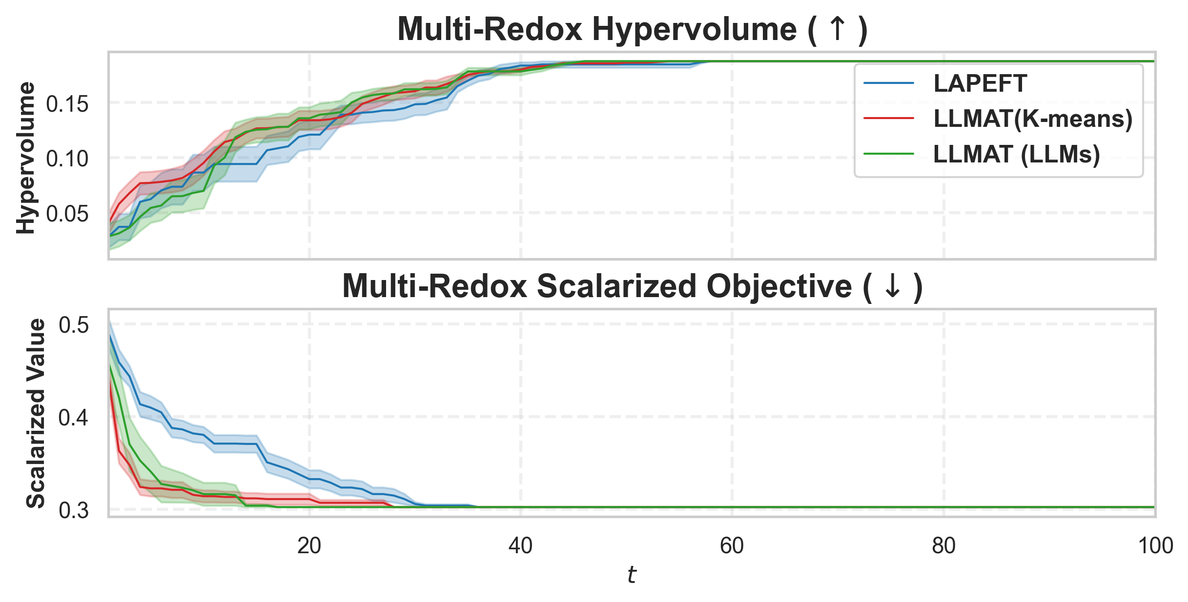
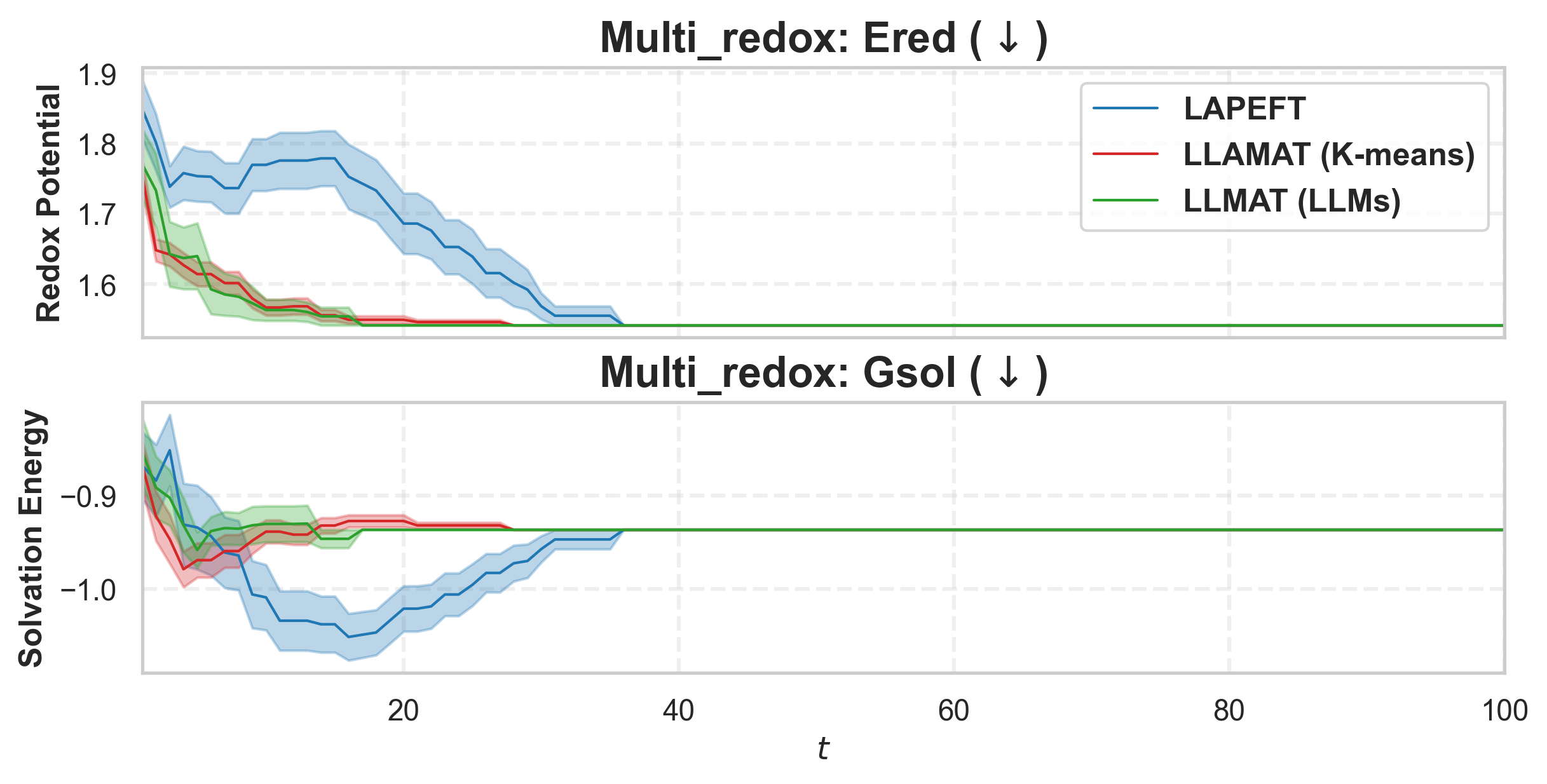
Figure 42: Multi-objective optimization for LAPEFT vs. LLMAT on the Redox-mer dataset: Upper & Lower Left: Hypervolume, scalarized objective. Right: Redox potential and solvation energy.

Due to space limitations, additional ablation studies on label noise, the quantile $\gamma$ and the extension to multi-objective optimization are provided in Fig. 38, Fig. 40, and Fig. 42 in the Appendix, respectively.

6 Conclusion

In this paper, we introduced LLMAT, a novel surrogate-free BO algorithm that incorporates LLM and foundation model features to inform the design and effectiveness of acquisition functions in BO. Our method also introduces a learned hierarchical partitioning scheme, using Monte Carlo Tree Search with tree nodes defined by shared binary classifiers to learn local acquisition functions that are informed by LLM priors. By incorporating shared parameters and meta-learning across these binary classifiers, LLMAT achieves better AF generalization in low-data regimes and enables efficient exploration of the vast search spaces of molecules. Extensive evaluations on six chemistry datasets demonstrate that LLMAT consistently outperforms baselines, highlighting the value of incorporating general LLMs and domain-specific foundation models with principled algorithmic design for molecular discovery.

Appendix

Appendix A Additional Background

A.1 Indirect Estimation of Acquisition Functions

Based on the definition of the acquisition function in Eq.(1), it’s natural to first calculate the predictive posterior $p(y|x,\mathbf{D}_{t})$, then estimate the AFs given the selected utility functions. In the following, we introduce two typical surrogate models that are non-parametric and parametric, respectively.

Gaussian Process (GP).

A typical choice of a non-parametric surrogate model $\hat{f}(x)$ is a GP with $p(\hat{f}(x)|\mathbf{D}_{t})={\mathcal{N}}(\mathbf{k}_{t}^{T}\mathbf{C}_{t}^{-1}\mathbf{y}_{t},k(x,x)-\mathbf{k}_{t}^{T}\mathbf{C}_{t}^{-1}\mathbf{k}_{t})$ being Gaussian given some kernel function $k(\cdot,\cdot)$, where $\mathbf{k}_{t}[i]=k(x_{i},x)\forall i\in[t]$, $\mathbf{K}_{t}[i,j]=k(x_{i},x_{j}),\forall i,j\in[t]$, and $\mathbf{C}_{t}=\mathbf{K}_{t}+\sigma^{2}\mathbf{I}_{t}$. In this case, the predictive posterior is tractable and has the form of $p(y|x,\mathbf{D}_{t})={\mathcal{N}}(\mathbf{k}_{t}^{T}\mathbf{C}_{t}^{-1}\mathbf{y}_{t},k(x,x)+\sigma^{2}-\mathbf{k}_{t}^{T}\mathbf{C}_{t}^{-1}\mathbf{k}_{t})$. However, the basic GPs have a ${\mathcal{O}}(t^{3})$ computational complexity for training, even sparse GPs still require ${\mathcal{O}}(t)$, posing difficulty to scale to a large dataset of observations.

Bayesian Neural Network (BNN).

If we consider parametric surrogate model $\hat{f}(x)=\text{NN}(\theta,x)$ with $\text{NN}(\theta,\cdot)$ being a predefined Neural Network (NN) of parameter $\theta$, then, the predictive posterior of BNN is $p(y|x,\mathbf{D}_{t})=\int p(y|x,\theta)p(\theta|\mathbf{D}_{t})d\theta$. The posterior $p(\theta|\mathbf{D}_{t})$ is often not analytically tractable. Hence, solutions like Laplace Approximation (LA), Variational Inference (VI) and Monte Carlo Sampling are often adopted to approximate the integral.

A.2 Parameter-Efficient Finetuning

Fine-tuning large pretrained models on downstream tasks often requires updating all model parameters, which can be computationally expensive and memory-intensive. Parameter-efficient fine-tuning (PEFT) methods aim to reduce this overhead by introducing a small set of trainable parameters while keeping the original pretrained model weights frozen.

Among various PEFT methods, Low-Rank Adaptation (LoRA) hu_lora_2021 has gained popularity due to its efficiency and effectiveness. LoRA hypothesizes that the update to the pretrained weight matrices can be approximated by a low-rank decomposition. Formally, consider a pretrained weight matrix $W_{0}\in\mathbb{R}^{d\times k}$ in a neural network (e.g., a linear layer or attention projection). Instead of updating $W_{0}$ directly, LoRA introduces two trainable matrices $A\in\mathbb{R}^{d\times r}$ and $B\in\mathbb{R}^{r\times k}$, where $r\ll\min(d,k)$ is the rank of the adaptation:

$$W=W_{0}+\Delta W=W_{0}+BA,$$

where $BA$ is a low-rank matrix capturing task-specific updates. During fine-tuning, $W_{0}$ is kept frozen, and only $A$ and $B$ are optimized. For an input $x\in\mathbb{R}^{k}$, the layer output becomes

$$y=Wx=W_{0}x+BAx.$$

To further control the magnitude of updates, a scaling factor $\alpha$ is often introduced:

$$W=W_{0}+\frac{\alpha}{r}BA,$$

where the factor $\frac{\alpha}{r}$ ensures the update has a similar scale across different rank settings. This formulation significantly reduces the number of trainable parameters from $d\times k$ to $r(d+k)$ while retaining strong adaptation capability.

A.3 Welch’s ANOVA

Suppose we have $k$ clusters, where cluster $i$ has sample size $n_{i}$, sample mean $\bar{x}_{i}$, and sample variance $\sigma_{i}^{2}$. Define the weights:

$$w_{i}=\frac{n_{i}}{\sigma_{i}^{2}},\quad i=1,\dots,k,$$

and the weighted mean:

$$\bar{x}_{w}=\frac{\sum_{i=1}^{k}w_{i}\bar{x}_{i}}{\sum_{i=1}^{k}w_{i}}.$$

The Welch F-statistic is then

$$F=\frac{\sum_{i=1}^{k}w_{i}(\bar{x}_{i}-\bar{x}_{w})^{2}}{(k-1)\left[1+\frac{2(k-2)}{k^{2}-1}\sum_{i=1}^{k}\frac{(1-w_{i}/\sum_{j}w_{j})^{2}}{n_{i}-1}\right]}.$$

The approximate degrees of freedom for the denominator is given by the Satterthwaite approximation:

$$\nu\approx\frac{k^{2}-1}{3\sum_{i=1}^{k}\frac{(1-w_{i}/\sum_{j}w_{j})^{2}}{n_{i}-1}}.$$

Finally, $F$ is compared against an $F$-distribution with $(k-1,\nu)$ degrees of freedom to compute the p-value.

A.4 Games-Howell Post-hoc Test

Suppose we have $k$ clusters, where cluster $i$ has sample size $n_{i}$, sample mean $\bar{x}_{i}$, and sample variance $\sigma_{i}^{2}$. For a pair of groups $(i,j)$, the test statistic is

$$t_{ij}=\frac{\bar{x}_{i}-\bar{x}_{j}}{\sqrt{\frac{\sigma_{i}^{2}}{n_{i}}+\frac{\sigma_{j}^{2}}{n_{j}}}}.$$

The degrees of freedom for this comparison are approximated using the Welch–Satterthwaite equation:

$$\nu_{ij}=\frac{\left(\frac{\sigma_{i}^{2}}{n_{i}}+\frac{\sigma_{j}^{2}}{n_{j}}\right)^{2}}{\frac{(\sigma_{i}^{2}/n_{i})^{2}}{n_{i}-1}+\frac{(\sigma_{j}^{2}/n_{j})^{2}}{n_{j}-1}}.$$

The p-value is computed from the $t$-distribution with $\nu_{ij}$ degrees of freedom:

$$p_{ij}=2\cdot\Big(1-T_{\nu_{ij}}(|t_{ij}|)\Big),$$

where $T_{\nu_{ij}}$ is the cumulative distribution function of the $t$-distribution. Optionally, a multiple comparison correction (e.g., Bonferroni) can be applied.

Appendix B Related Works

B.1 LLMs for Optimization.

Recent research has increasingly leveraged pretrained Large Language Models (LLMs) as informative priors in optimization tasks across a variety of domains. For instance, LLMs have been used to improve prompt optimization strategies by conditioning on query-dependent representations [sun_query-dependent_2024, yang_large_2024, guo_connecting_2024]. Other works have integrated LLMs into evolutionary algorithms, using them as generative operators to evolve prompts or candidate solutions [meyerson_language_2024, lehman_evolution_2022, chen_evoprompting_2023].In the context of Bayesian Optimization (BO), LLMs have also been employed to guide acquisition functions, either for hyperparameter tuning [liu_large_2024, zhang_using_nodate] or for scientific discovery tasks such as molecular optimization [kristiadi_sober_2024, ramos_bayesian_2023].

B.2 High-dimensional BO

Several approaches have been developed to scale BO to high-dimensional search spaces, including structural assumptions, subspace embedding, variable selection, and local modeling and space partitioning. wang_learning_2020, wang_sample-efficient_2021 progressively bifurcate the search space into more promising and less promising subspaces, starting with the full candidate space $\Omega$. K-means clustering is applied to observed data (features $x$ and values $y$) within each space to split the data into "good" and "bad" clusters based on the average values of the clusters. These labeled clusters are then used to train a Support Vector Machine (SVM) classifier, which produces a non-linear decision boundary to define latent actions for bifurcating the search space. Finally, local surrogate models for BO are trained on observed data in the selected subspace via Upper Confidence Bound (UCB). Based on wang_learning_2020, li_navigating_2025 propose to reweigh the samples in different partition by their UCB values without constraining sampling to certain partitions. In contrast, we do not separately use SVMs for partitioning and additional models for acquisition function estimation.

We focus on leveraging LLM-derived priors to enhance high-dimensional Bayesian Optimization (BO) for molecular discovery by using LLMs for feature extraction, finetuning and prompting for clustering. Unlike prior work, we introduce a shared neural network classifier that simultaneously partitions the candidate space and estimates acquisition functions at each tree node, effectively amortizing both tasks. To further improve data efficiency, we adopt a meta-learning [chen_generalization_2021, chen_stability-plasticity_2023] approach that amortizes classifier training across nodes, enabling more stable learning in early data-scarce stages. Moreover, while previous methods assume a continuous search space and rely on rejection sampling, they fail in discrete settings where selected regions may contain no valid candidates. We address this limitation via a backtracking strategy. Our method traverses a UCB-guided path through the search tree, estimating local acquisition functions from leaf to parent until valid candidates are found. In the worst case, it returns to the original Likelihood-Free BO (LFBO) approach.

Appendix C Clustering Prompts

C.1 Redoxmer

C.2 Solvation

C.3 Kinase

C.4 Photovoltaics

C.5 Laser

C.6 Photoswitches

C.7 Variations in Prompt

We ask ChatGPT to generate 4 alternative prompts based on our original prompt, the cluster label disagreements, the label distributions, and the generated prompts are listed below.

Appendix D Experimental Details

We follow most of the settings in kristiadi_sober_2024 for using the foundation models and baselines: GP and Laplace, while we Refactored their code presented in repo https://github.com/wiseodd/lapeft-bayesopt for better extension.

Computational Resource

The experiments were conducted on multiple server nodes, each equipped with 6 CPUs and a single GPU with 32 GB of memory. To obtain results faster, the experiments were run across different clusters. We ensured that, for each dataset, all algorithms were tested on the same type of CPU and GPU.

D.1 Foundation Models

Features and Prompts for Foundation Model.

For the LLM features, we average the last transformer embeddings along the sequence dimension, ignoring padding and EOS tokens. All LLM-related components in this work were implemented using the Hugging Face Transformers library wolf_huggingfaces_2019. We use the single SMILES string as the prompt input for feature extraction and parameter-efficient finetuning of these foundation models.

D.2 BO on Fixed-features

We use the same batch size 256 for AFs estimation (i.e., prediction) for all the algorithms.

D.2.1 Training Details

GP

For GP, we use BoTorch [balandat_botorch_2020], with the Tanimoto kernel from Gauche [griffiths_gauche_2023]. The marginal likelihood is optimized using Adam [kingma_adam_2014] with a learning rate of 0.01 for 500 epochs.

Laplace

A 2-hidden-layer multilayer perceptron with 50 units per layer is used. The network is optimized with Adam at a learning rate of $1\times 10^{-3}$ and weight decay $5\times 10^{-4}$ for 500 epochs with batch size 20, using cosine annealing for the learning rate [loshchilov_sgdr_2016]. The Laplace approximation is applied post hoc, with prior precision tuned via marginal likelihood for 100 iterations. The Hessian is approximated using a Kronecker structure [ritter_scalable_2018].

LLMAT

We build the MCTs that satisfy the tree depth and minimal leaf sample size constraints. Then we train classifiers that are 2-hidden-layer multilayer perceptrons with 50 units per layer using ReLU activation. The classifiers are trained with Adam of learning rate $1\times 10^{-2}$ and weight decay $5\times 10^{-4}$ for 50 epochs with batch size $256$. Other hyperparameters like the quantile $\gamma$, the $\lambda$ for UCB, the meta-learning rate $\eta$, the threshold for partitioning, the tree depth, and the p-value are summarized in Tab. 1.

Table 1: Hyperparameter Configuration

Category	Parameter	Value
General	$\gamma$	0.5
	$\lambda$	0.5
	$\eta$	0.005, 0.01
	tree_depth	3
	p_val	0, 0.01, 0.05
	threshold	0.5
Fix Args	batch_size	256
	Head Parameters:
	n_epochs	50
	learning rate	1e-2
	batch_size	256
	leaf_sample_size	2

D.3 BO with PEFT

We keep the same LoRA configuration for our algorithm and the Laplace baseline. The batch size for acquisition function estimation was set to $16$ for T5-Chem and $32$ for Molformer. Same batch size was also used for LoRA training.

LoRA Configuration.

We used LoRA with rank 4, applied without bias on the key and value attention weights. The scaling factor $\alpha$ was set to 16, and dropout with probability 0.1 was applied. We followed the implementation from HuggingFace’s PEFT library [mangrulkar_peft_2022].

D.3.1 Training details of Laplace

In kristiadi_sober_2024, the following setting was applied to PEFT with Laplace Approximation.

LoRA Training.

The LoRA parameters and the regression head were jointly trained using AdamW with learning rates of $3\times 10^{-4}$ and $1\times 10^{-3}$ for the LoRA and regression head weights, respectively (except for the Photoswitch dataset, where they used $3\times 10^{-3}$ and $1\times 10^{-2}$). Training was performed for 50 epochs with weight decay 0.01. Subsequently, the regression head was optimized for 100 epochs under the same hyperparameters.

Laplace Approximation.

The Laplace approximation was applied to both the LoRA and regression head weights. We used a Kronecker-factored Hessian and optimized the layerwise prior precisions with post hoc marginal likelihood for 200 iterations, following daxberger_laplace_2021.

D.3.2 Training details of our algorithm

Following the fixed-feature setting, we construct MCTs subject to tree-depth and minimum leaf-sample constraints, and train 2-layer MLP classifiers (50 hidden units per layer, ReLU activations). To enable larger classifier batch sizes, batching is applied after the feature extractor and LoRA layers. Classifiers are trained with Adam (lr $1\times 10^{-2}$, weight decay $5\times 10^{-4}$, batch size 256, 50 epochs). LoRA learning rates are task-specific: $3\times 10^{-5}$ (Solvation, Kinase), $5\times 10^{-5}$ (Redoxmer, Laser), and $1\times 10^{-7}$ (Photovoltaics, Photoswitch). Additional hyperparameters, including $\gamma$, $\lambda$, $\eta$, partitioning threshold, tree depth, and $p$-value, are listed in Tab. 1.

Table 2: Hyperparameter Configuration

Category	Parameter	Value
PEFT	batch_size	16, 32
	Head Parameters:
	n_epochs	50
	learning rate	1e-2
	batch_size	256
	leaf_sample_size	2
	LoRA Parameters:
	n_epochs	50
	learning rate	3e-5, 5e-5, 1e-7
	batch_size	16, 32

Appendix E Additional Experimental Results

In this section, we present additional experimental results on historical optimums, GAP metrics, regret, and computational costs for each dataset based on T5-chem and Molformer.

E.1 Fixed-feature results for more foundation models

E.1.1 Historical optimums

E.1.2 Computation Time

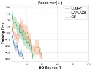
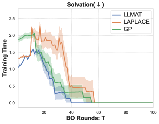
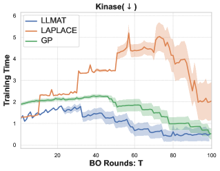
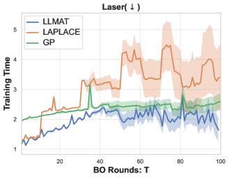
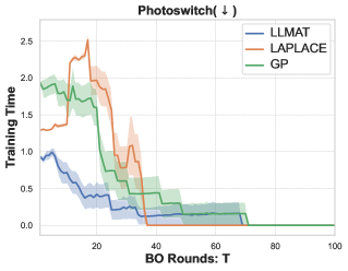
Figure 12: Training time comparison on different chemistry datasets with T5-Chem model.

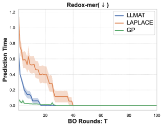
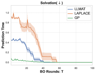
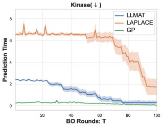
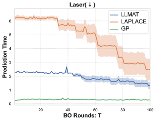
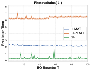
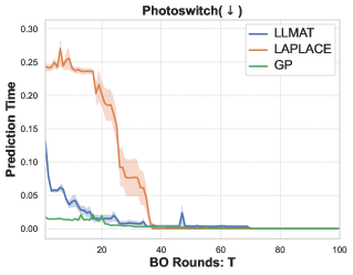
Figure 13: Prediction time comparison on different chemistry datasets with T5-Chem model.

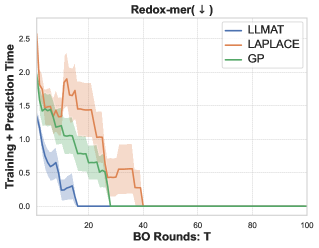
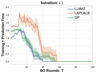
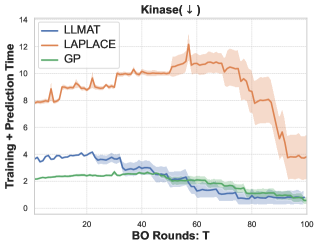
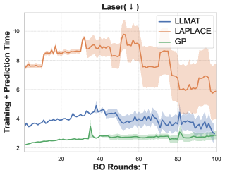
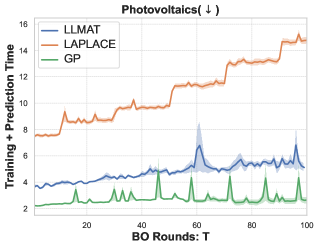
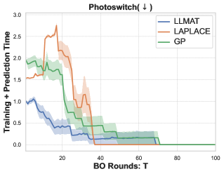
Figure 14: Overall time comparison on different chemistry datasets with T5-Chem model.

E.2 Fixed and finetuned results for T5-chem Model

E.2.1 Historical optimums

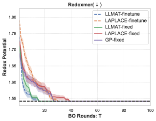
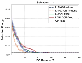
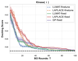
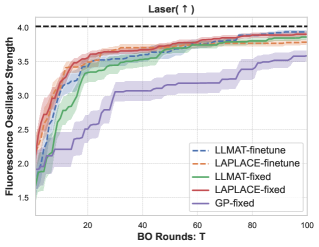
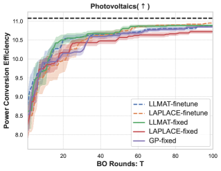
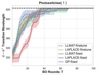
Figure 15: Historical optimums comparison on different chemistry datasets using T5-Chem model.

E.2.2 GAP metric

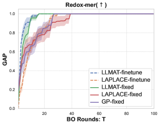
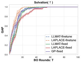
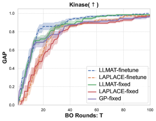
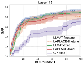
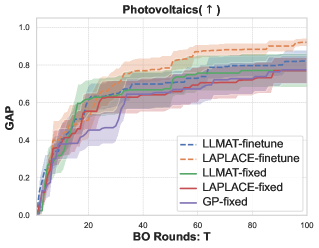
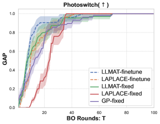
Figure 16: GAP comparison on different chemistry datasets with T5-Chem model.

E.2.3 Average Regret

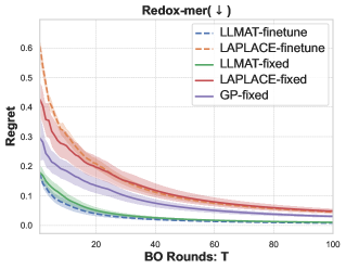
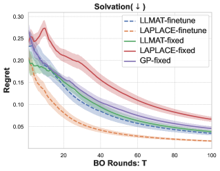
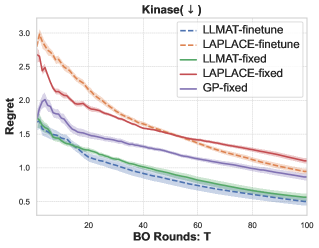
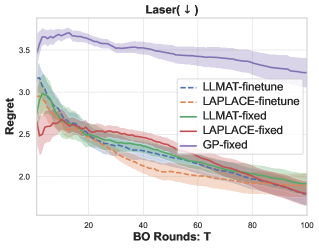
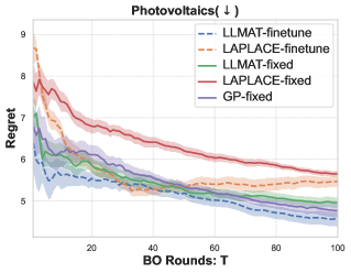
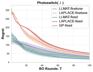
Figure 17: Regrets comparison on different chemistry datasets using T5-Chem model.

E.2.4 Computation time for PEFT

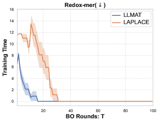
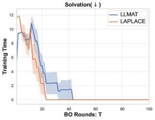
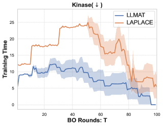
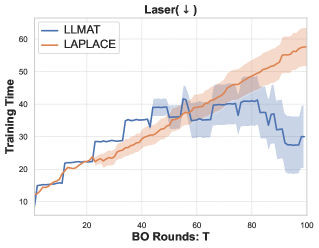
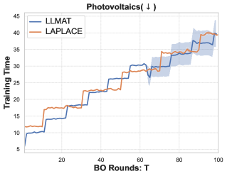
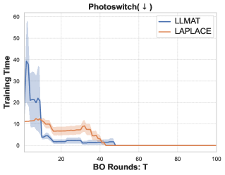
Figure 18: Training time comparison on different chemistry datasets with T5-Chem model.

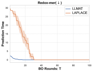
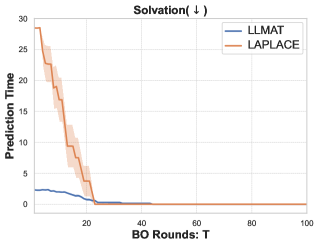
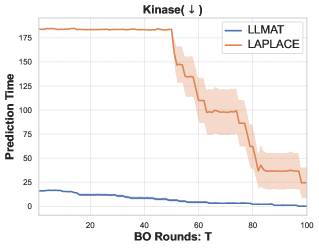
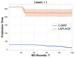
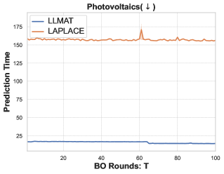
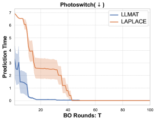
Figure 19: Prediction time comparison on different chemistry datasets with T5-Chem model.

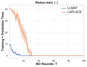
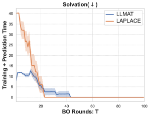
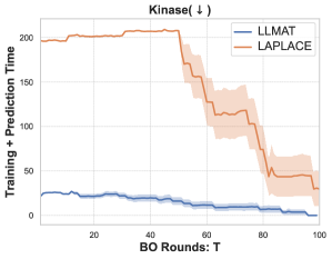
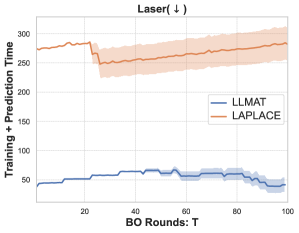
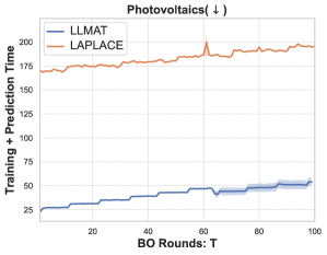
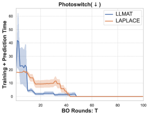
Figure 20: Overall time comparison on different chemistry datasets with T5-Chem model.

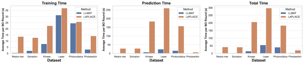
Figure 22: BO time for different datasets on finetuning T5-Chem model with LoRA.

E.3 Fixed and finetuned results for Molformer

E.3.1 Historical optimums

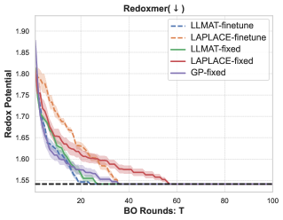
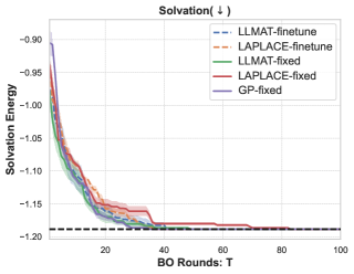
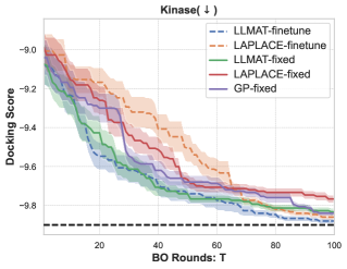
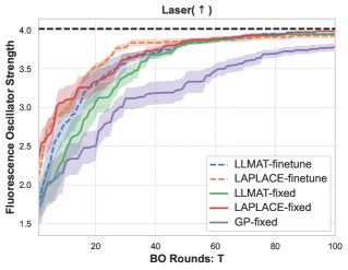
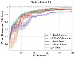
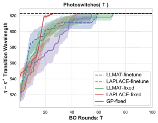
Figure 23: Historical optimums comparison on different chemistry datasets using Molformer.

E.3.2 Average regrets

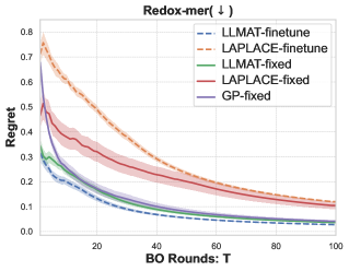
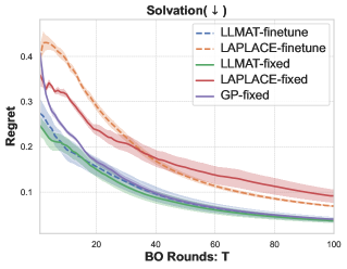
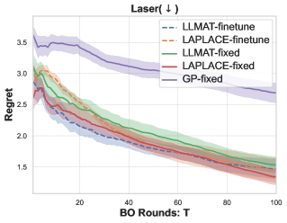
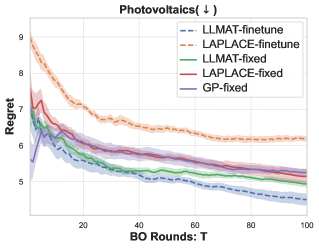
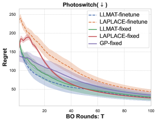
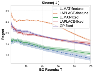
Figure 24: Regrets comparison on different chemistry datasets using Molformer.

E.3.3 GAPs

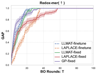
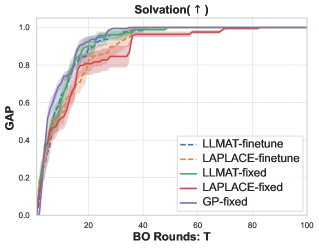
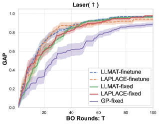
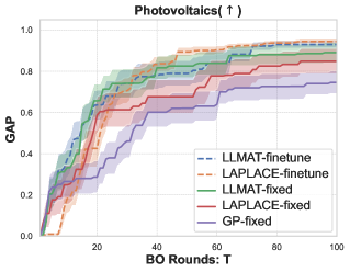
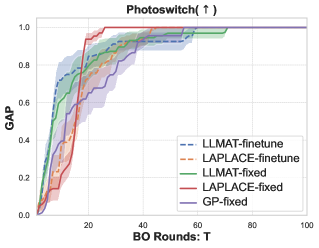
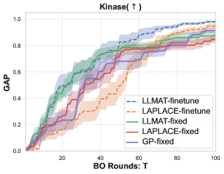
Figure 25: GAPs comparison on different chemistry datasets using Molformer

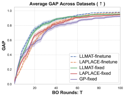
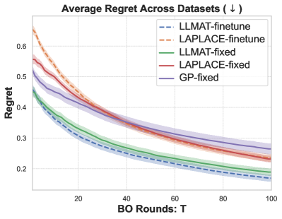
Figure 26: Average GAPs and regrets across all the datasets on finetuning and fixed Molformer.

E.4 Clustering results

E.4.1 K-means clustering

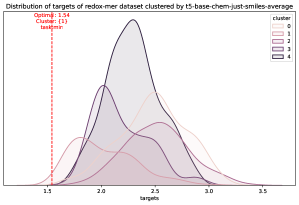
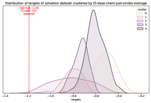
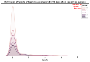
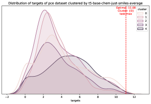
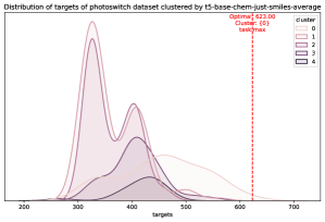
Figure 27: Distribution of property values for K-means clusters on features extracted from T5-Chem.

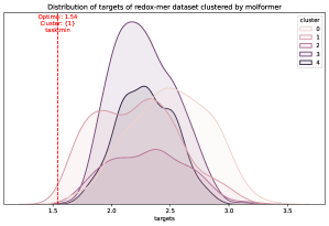
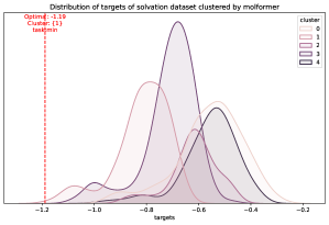
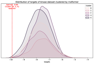
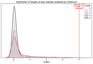
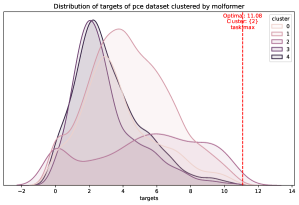
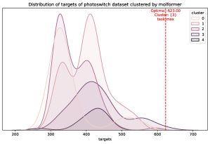
Figure 28: Distribution of property values for K-means clusters on features extracted from Molformer.

E.4.2 LLM-based clustering

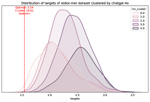
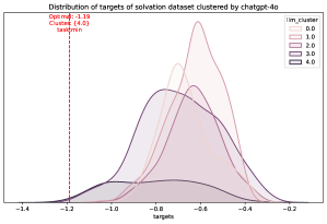
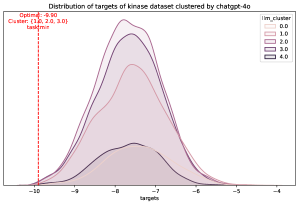
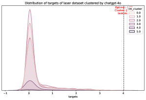
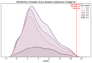
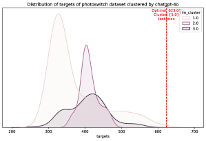
Figure 29: Distribution of property values for ChatGPT-based clustering results.

E.5 Ablation on p-values

In this section, we provide additional details on how varying the p-values impacts our proposed algorithm in terms of the GAP metric, average regret, and prediction time per BO round for each dataset, using both K-means and LLM-based clustering. The results suggest that the LLM-based clustering approach is significantly effective in reducing prediction time while at the same time improving or maintaining the GAP and regret performance for Redoxmer, Solvation, and Photovoltaics, reflecting that ChatGPT-4o has informative knowledge on these datasets. This is consistent with its clustering visualization in Fig. 1, where the mean property values for clusters have an obvious difference. K-means clustering is effective for Redoxmer and Solvation in reducing prediction time without degrading the performance.

E.5.1 GAPs’ change w.r.t different p-values

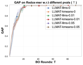
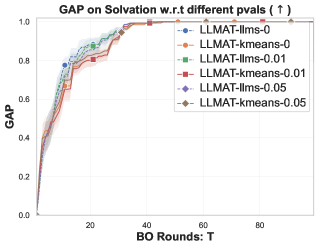
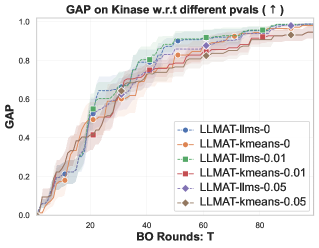
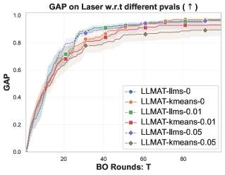
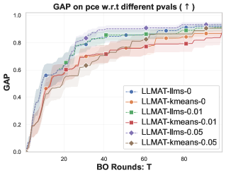
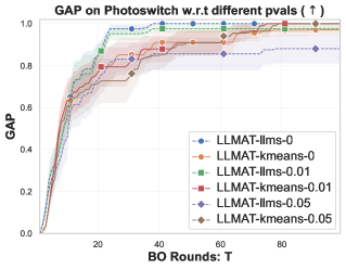
Figure 30: GAPs’ change for different clustering approach and p-values using Molformer.

E.5.2 Regrets change w.r.t different p-values

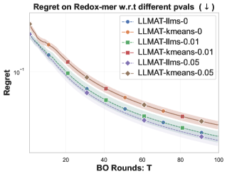
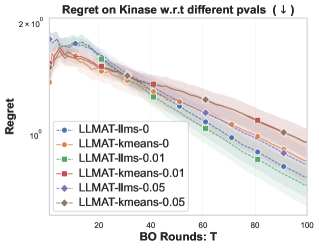
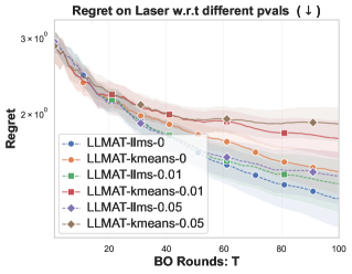
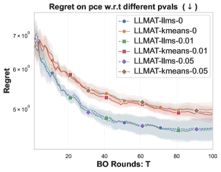
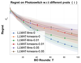
Figure 31: Regrets’ change for different clustering approach and p-values with Molformer.

E.5.3 Effects on reducing prediction time w.r.t different p-values

E.6 Toy Data

E.6.1 Levy-1D Data

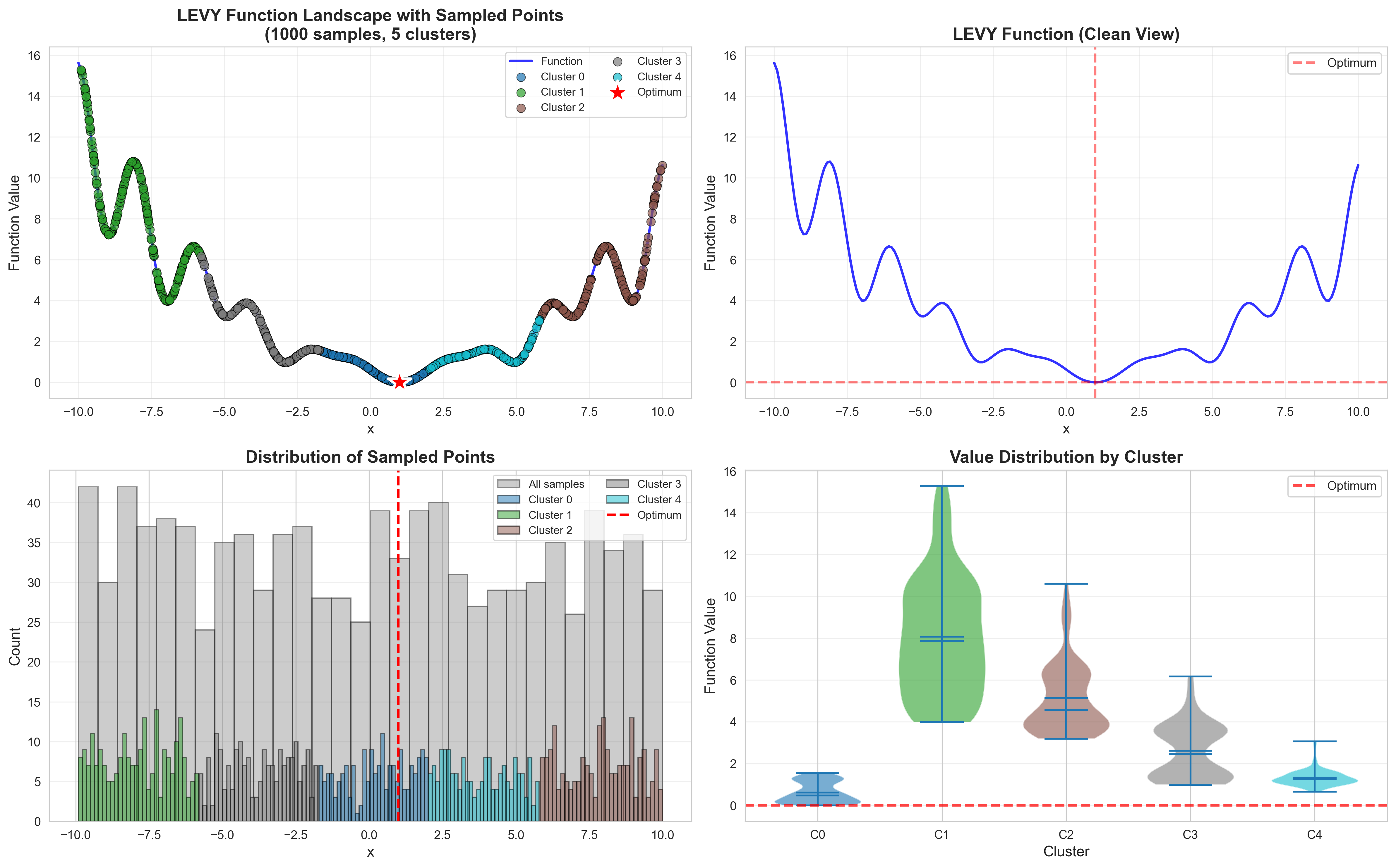
Figure 33: Illustration $1000$ samples of Levy-1D function with K-means clustering.

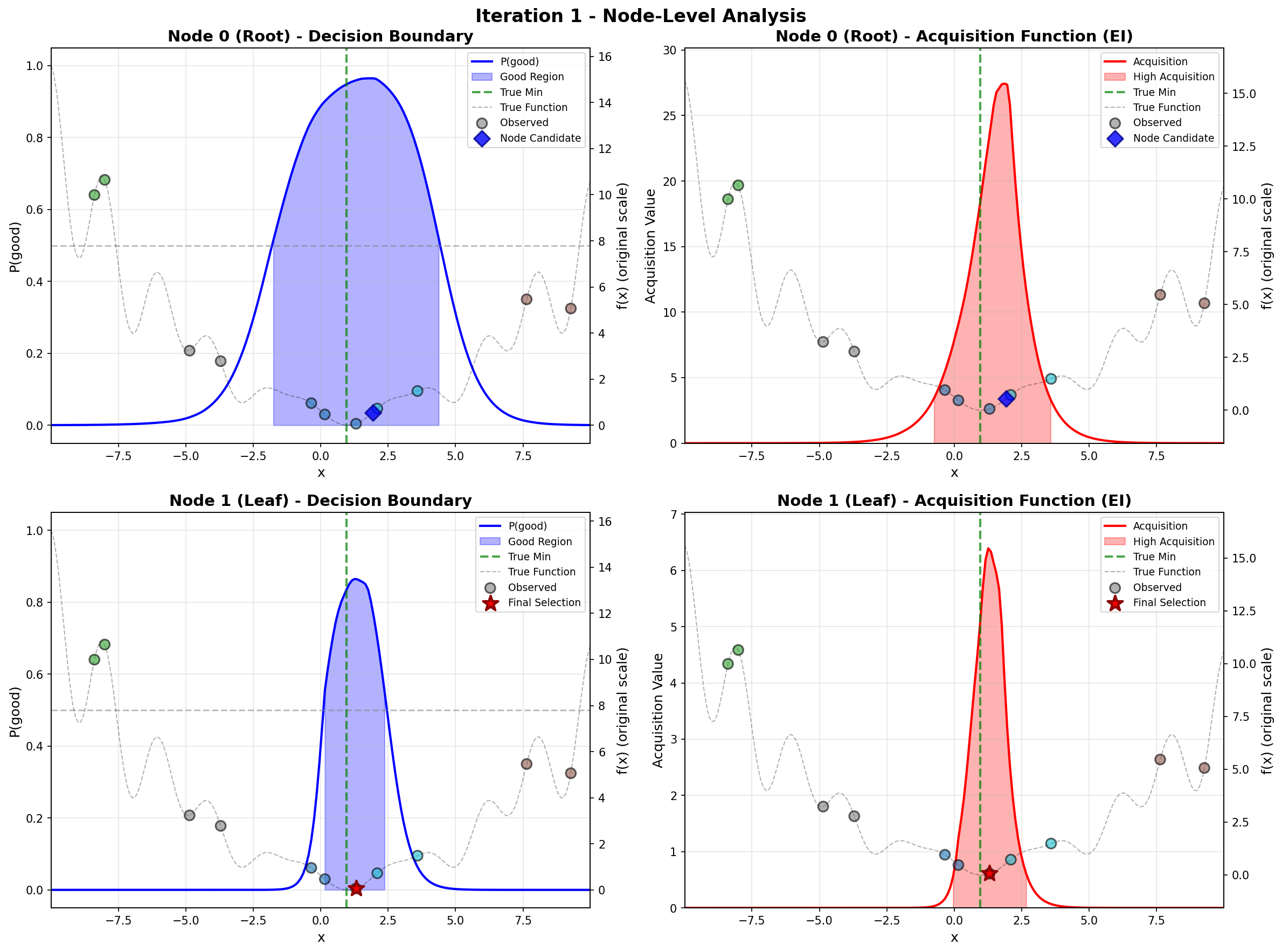
Figure 34: Refined AFs in LLMAT enable more efficient BO (Iteration 1).

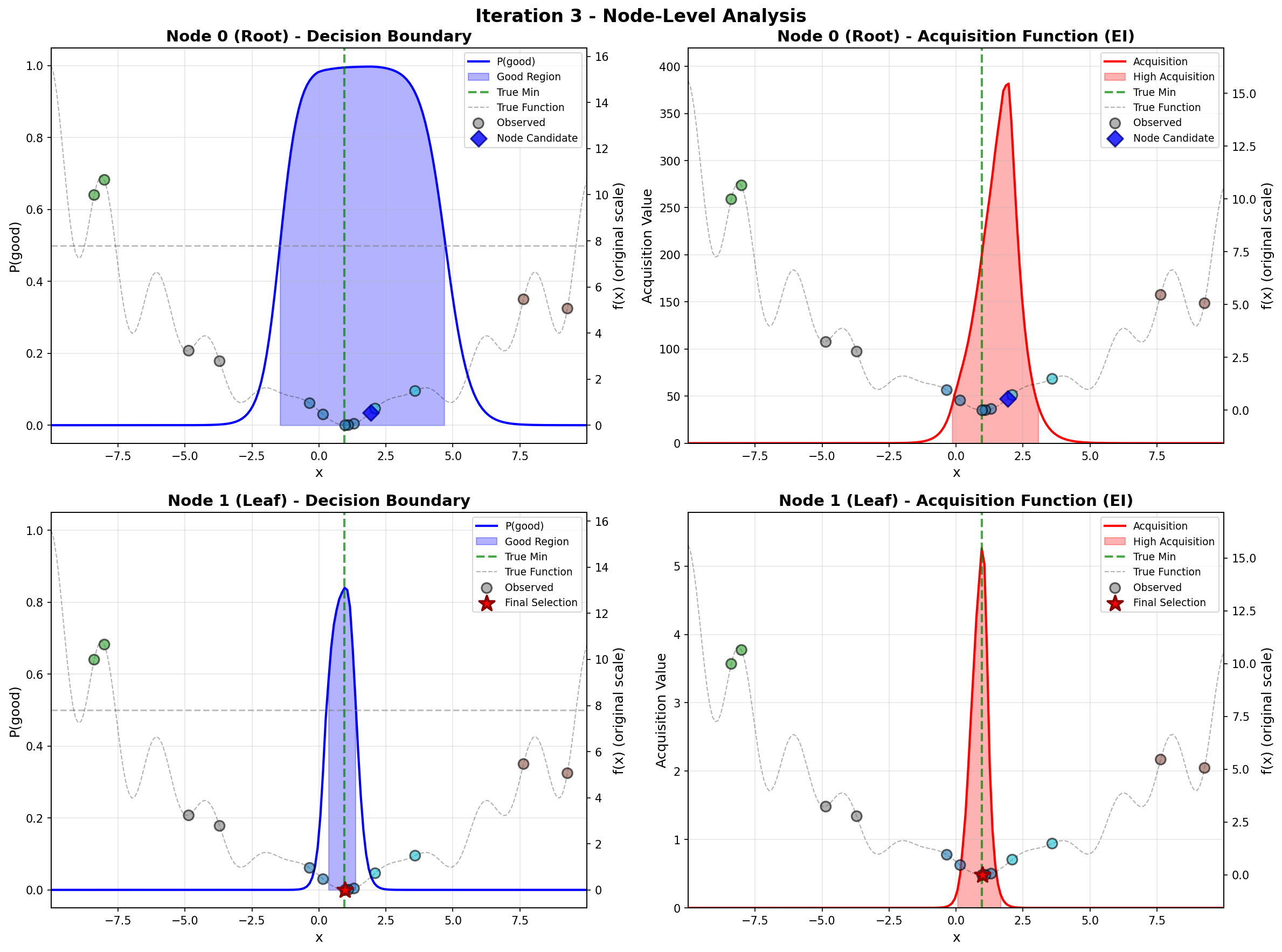
Figure 35: Refined AFs in LLMAT enable more efficient BO (Iteration 3).

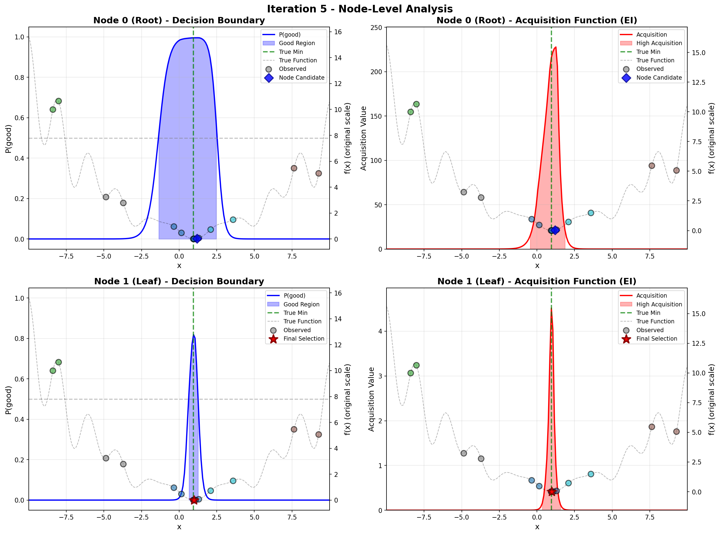
Figure 36: Refined AFs in LLMAT enable more efficient BO (Iteration 5).

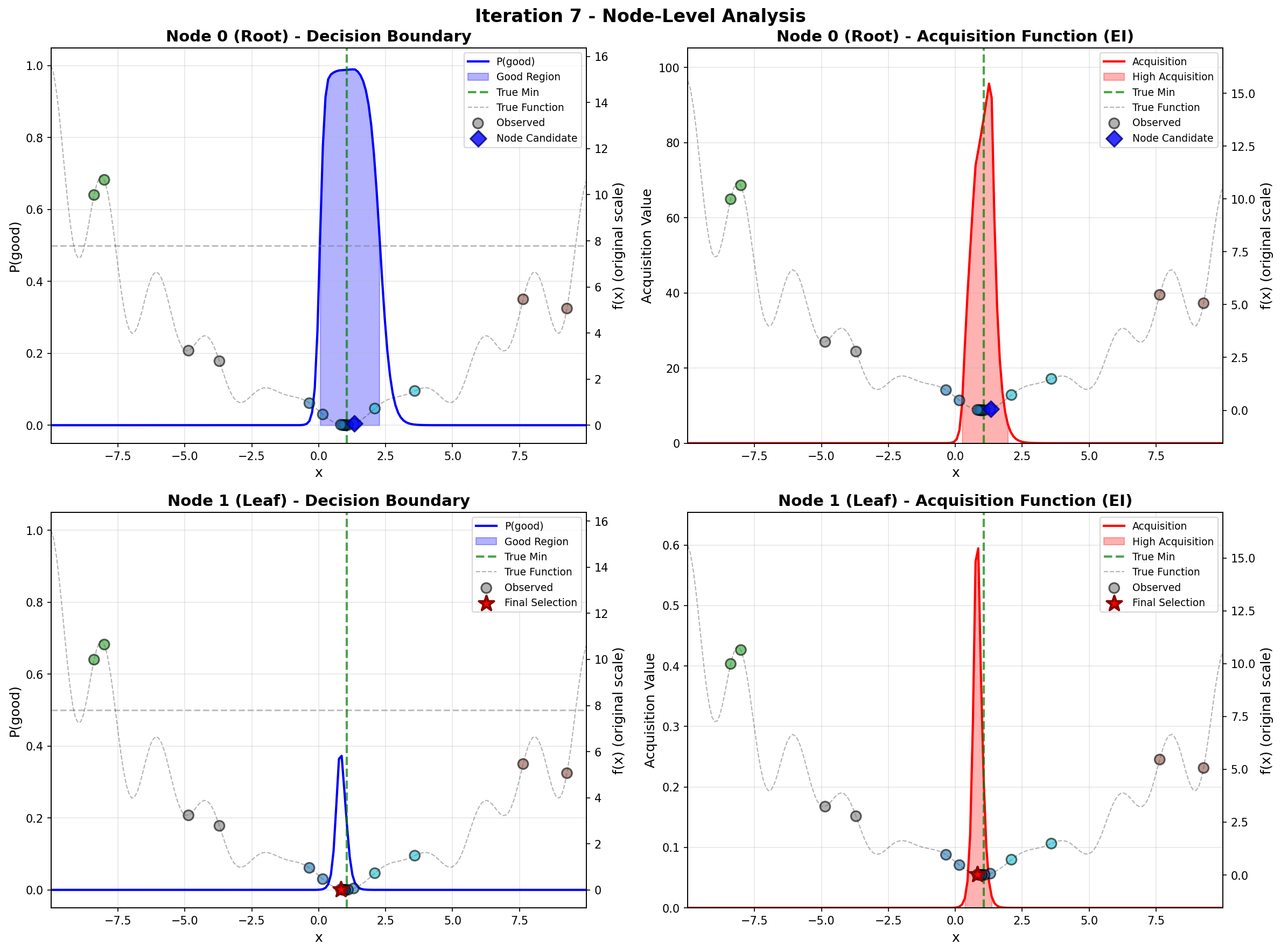
Figure 37: Refined AFs in LLMAT enable more efficient BO (Iteration 7).

E.6.2 Levy-10D Data

E.6.3 Ablation of $\gamma$

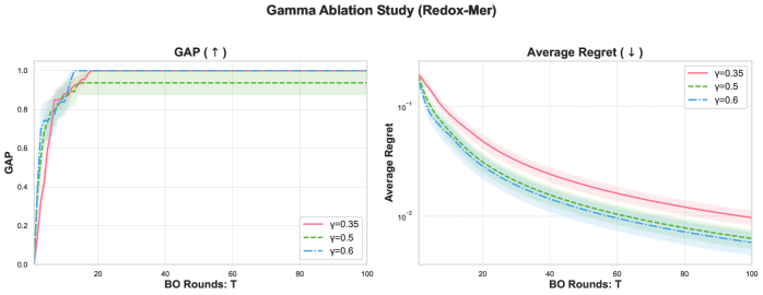
Figure 39: Illustration of LLMAT Performance Change w.r.t Different $\gamma$s.

E.6.4 Additional results for Llam2-7b

E.7 Multi-objective Optimization Extension

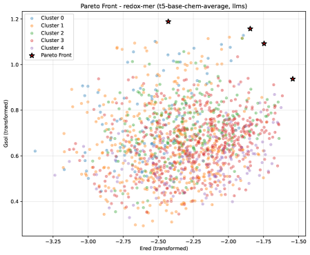
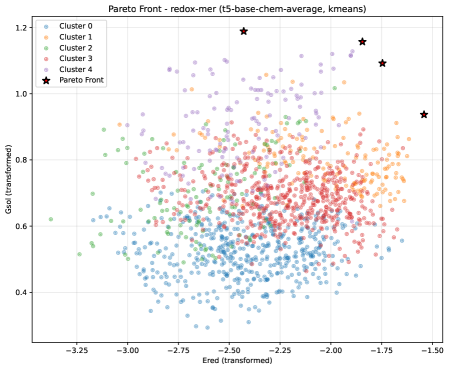
Figure 41: Illustration of Pareto fronts and LLMs and K-means clusters on Multi-Redox Data.

Appendix F Limitations and Claims

Limitations

In this paper, the LLM-clustering method is evaluated using simple prompts to GPT-4o, though it could be extended to other models such as GPT-5 or DeepSeek R1, or enhanced with explicit chain-of-thought designs. The prompts could also be refined by incorporating queries alongside the initial datasets. However, given the complexity of the current study, these extensions are left for future work.

Broader Impacts

• Potential Positive Impacts. The proposed methods can accelerate molecular discovery by leveraging knowledge from both general LLMs and domain-specific foundation models. They can be combined with generative approaches to propose novel, unseen molecules for drug and material design, offering significant societal benefits: new drugs may save lives, and new materials could contribute to environmental protection.

• Potential Negative Impacts. However, the method also carries potential risks. For example, the same capabilities could be misused to create toxic or harmful compounds, and overreliance on AI predictions without rigorous experimental validation could lead to unintended consequences. Responsible use, careful oversight, and appropriate safety measures are therefore critical.

Precise Use of Large Language Models (LLMs)

We use LLMs as grammar correction tools and for improving written text flow, combined with human proofreading. No LLM was used for the idea or primary text of the paper. However, as this paper investigates how LLMs can help inform acquisition functions for BO over molecular datasets, we incorporate LLMs as algorithmic modules, where we also prompt chatGPT to generate proper LLM-clustering prompts.