The Interplay of Statistics and Noisy Optimization: Learning Linear Predictors with Random Data Weights
Abstract
We analyze gradient descent with randomly weighted data points in a linear regression model, under a generic weighting distribution. This includes various forms of stochastic gradient descent, importance sampling, but also extends to weighting distributions with arbitrary continuous values, thereby providing a unified framework to analyze the impact of various kinds of noise on the training trajectory. We characterize the implicit regularization induced through the random weighting, connect it with weighted linear regression, and derive non-asymptotic bounds for convergence in first and second moments. Leveraging geometric moment contraction, we also investigate the stationary distribution induced by the added noise. Based on these results, we discuss how specific choices of weighting distribution influence both the underlying optimization problem and statistical properties of the resulting estimator, as well as some examples for which weightings that lead to fast convergence cause bad statistical performance.
1 Introduction
Gradient descent with random weightings of the data points is a ubiquitous method in the training of large machine learning models. For example, during each iteration of training, stochastic gradient descent (SGD) randomly selects a mini-batch of the data on which to compute the gradient, which may be interpreted as a random weighting with binary outcomes. This yields computational gains if the batch size is relatively small in comparison with the entire data set. The most basic instance of SGD features a fixed batch size and uniform inclusion probability for each data point, but some variants use random batch sizes [bieringer_kasieczka_et_al_2023] and/or weighted probabilities [needell_srebro_et_al_2014, needell_ward_2017, csiba_richtarik_2018].
While these methods were invented to make otherwise computationally intractable problems accessible, they also induce a regularizing effect on the problem [smith_dherin_et_al_2021, wu_su_2023]. This effect, termed implicit regularization, has recently experienced interest in the context of generalization [zhang_bengio_et_al_2017, zhang_bengio_et_al_2021]. In empirical risk minimization (ERM), generalization refers to the ability of an estimate to accurately predict the labels of previously unseen data. Non-convex risks, such as those associated with heavily over-parametrized deep neural networks, may admit many qualitatively different local and global minima, only some of which generalize. Implicit regularization through the chosen optimization method has been put forward as one plausible explanation for the effectiveness of ERM in producing large machine learning models that generalize [bartlett_montanari_et_al_2021].
One of the ways that random weighting of the data points influences the computed parameter estimates concerns the diffusion of the iterates through the parameter space. As an example, consider the empirical risk
with representing the loss on the th data point. For a given initialization , the classical SGD recursion takes the form , with and step-size . The conditional expectation of matches , so the long-run distribution of clusters around the critical points of under mild assumptions [azizian_iutzeler_et_al_2024]. The variance induced through the random sampling of the may help the SGD algorithm in escaping sharp local minima [ibayashi_imaizumi_2023], which leads to better generalization guarantees [haddouche_viallard_et_al_2025].
In the example above, the added noise does not change the conditional expectation of the gradient, but this may not always be the case. For biased sampling of the , the long-run distribution of the iterates will cluster around the critical points of the weighted empirical loss, with each weighted according to the probability of . Biased sampling may be desirable if some of the observed data points hold a stronger influence on the overall loss than others [needell_srebro_et_al_2014, needell_ward_2017]. In this case, the noise changes the underlying loss surface and hence the resulting trajectory of the SGD iterates.
In the present article, we focus on linear regression as a well-understood model and analyze the impact of random weightings on the underlying gradient descent dynamics. While the linear model does not capture the complexities associated with non-convex ERM, it serves as a useful starting point to characterize the induced regularization. Further, SGD with biased sampling in this model features a striking relationship with randomized algorithms for the solution of linear systems [needell_srebro_et_al_2014]. On the technical side, we adapt recent progress in the analysis of linear regression with dropout [clara_langer_et_al_2024, li_schmidt-hieber_et_al_2024], with the aim of characterizing the interactions between gradient descent dynamics and the added variance, as well as the resulting stationary distribution. Throughout, we provide a unified analysis for generic random weightings, meaning the distribution is not limited to discrete outcomes. Continuous weightings may be desirable to down-weight outliers and increase robustness, both in classical statistics [holland_welsch_1977] and modern machine learning [de_brabanter_de_brabanter_2021, ren_zeng_et_al_2018]. Further, continuously-valued random data weights relate to curriculum learning [bengio_weston_2009] and randomized sketching methods [vempala_2004].
The article is organized as follows: Section 2 gives a short overview of gradient descent in the linear model and discusses the relationship between weighted linear least squares (W-LLS) and random weightings. Section 3 details our convergence analysis of randomly weighted gradient descent. Section 4 discusses specific weighting strategies and their influence on both optimization and statistical properties of the algorithm. Section 5 concludes with further discussion of future research directions. The proofs of all numbered statements are deferred to the appendices.
1.1 Related Work
The idea of approximating an iterative optimization algorithm via random sampling finds its genesis in [robbins_monro_1951], often considered as having founded the study of stochastic approximation methods. Motivated by questions in machine learning, far ranging generalizations of classical stochastic approximation results have recently been obtained [davis_drusvyatskiy_et_al_2020, fehrman_gess_et_al_2020, mertikopoulos_hallak_et_al_2020, dereich_kassing_2024]. While we do not use these abstract convergence theorems, our results may be seen as concrete counterparts to such theorems that exploit the precise structure of the linear model as much as possible.
As a widely used method, SGD has inspired many studies, so we only summarize the most relevant directions of research. The batch size, as a tuning parameter, controls the variance of the gradient estimators and hence directly influences the training dynamics [wilson_martinez_2003]. For a weight-tied non-linear auto-encoder, [ghosh_frei_et_al_2025] show that the limit reached by SGD depends directly on the batch size. Biased sampling represents a further way to alter the dynamics, which may lead to faster convergence and connects to the randomized Kaczmarz method for linear systems [needell_srebro_et_al_2014]. One may also sample mini-batches with biased inclusion probabilities, with a natural sampling rule being proposed in [needell_ward_2017]. In a similar setting, [csiba_richtarik_2018] analyze the convergence of a stochastic dual coordinate ascent algorithm with importance sampling.
Toy model analysis of regularization induced by optimization algorithms is an active area of research. As shown in [bartlett_long_et_al_2023], sharpness-aware minimization forces the GD algorithm to asymptotically bounce between two opposing sides of a valley when applied to a quadratic objective. For diagonal linear networks trained with a stochastic version of SAM, [clara_langer_et_al_2025] compute the exact induced regularizer, which leads to exponentially fast balancing of the weight matrices along the GD trajectory. [wu_bartlett_et_al_2025] provide excess risk bounds for early stopping in logistic regression and investigate connections to explicit norm regularization. [clara_langer_et_al_2024] analyze the implicit and explicit regularizing effect of dropout in linear regression and [li_schmidt-hieber_et_al_2024] prove uniqueness of the induced stationary distribution and a quenched central limit theorem for the averaged iterates in the same setting.
For constant step-sizes, noisy GD algorithms produce iterates that diffuse through the parameter space indefinitely, unless the noise vanishes as the iterates approach a stable point. The resulting long-run distribution of the iterates reflects the geometry of the loss surface by clustering near critical points and may be shown to visit flat regions with higher frequency [azizian_iutzeler_et_al_2024]. [shalova_schlichting_et_al_2024] exhibit the asymptotic constraints induced by arbitrary noise in the small step-size limit. Ergodicity and asymptotic normality of the SGD iterate sequence for a non-convex loss is shown in [yu_balasubramanian_et_al_2021].
1.2 Notation
We let , , and signify the transpose, trace, and pseudo-inverse of a matrix . The maximal and minimal singular values of a matrix are denoted by and , with signifying the smallest non-zero singular value. For matrices of the same dimension, gives the element-wise product .
Euclidean vectors are always written in boldface and endowed with the standard norm . Given a matrix of suitable dimension, whenever . The orthogonal complement of contains all vectors satisfying for every ; we then also write .
Let and be non-trivial normed vector spaces, then the operator norm of a linear operator is given by . When and , the operator norm of a matrix matches and is also known as the spectral norm. We will drop the sub-script in this case, meaning .
For probability measures and on with sufficiently many moments, we denote by , the transportation distance
where the infimum is taken over all probability measures on with marginals and .
Given any two functions , as , signifies that .
2 Estimating Linear Predictors with Gradient Descent
Given a sample , of data points with corresponding labels , we aim to learn a linear predictor such that for each . We will focus on predictors learned via minimization of the empirical risk
| (1) |
Write for the length vector with entries and for the -matrix with rows , then, up to the constant factor , the empirical risk coincides with the linear least squares objective
| (2) |
From this point on, we absorb the factor into the observed data and labels and work with the loss (2). To keep notation compact, define the shorthand . If exists, then (2) admits the unique minimizer , known as the linear least squares estimator. The matrix defines a pseudo-inverse for , see [campbell_meyer_2009]. For singular , the definition of this estimator may be extended to take the value , with any generalization of the pseudo-inverse. In this case, admits many different pseudo-inverses, which lead to distinct estimators. We will choose a particular one so that coincides with the unique minimum-norm minimizer of (2), see Appendix D.1 for more details.
2.1 Noiseless Gradient Descent in the Overparametrized Setting
We briefly discuss minimization of the linear least squares objective via full-batch gradient descent. Fixing a sequence of step-sizes the gradient descent recursion generated by (2) takes the form
started from some initial guess . Expanding the norm in (2) yields the quadratic polynomial , with second derivative . Consequently, the objective is -strongly convex for invertible . Provided that for every and , this implies convergence of to the unique global minimizer , regardless of initialization. For singular , such as in the over-parametrized regime with , the objective (2) is merely convex, but an analogous convergence result holds under additional assumptions. The gradient of (2) evaluates to , so together with the property of the pseudo-inverse (Lemma D.1(a)), we can rewrite the gradient descent recursion as
| (3) |
For a suitably chosen initial point , the difference always lies in a sub-space on which each matrix acts as a contraction, ensuring convergence of to as . A precise result is given in the following classical lemma.
Lemma 2.1.
Suppose and , then
for every . Provided that , the left-hand side in the previous display vanishes as .
The fact that converges to the minimizer of (2) with the smallest magnitude appears in Section 3 of [bartlett_montanari_et_al_2021] as an example of implicit regularization through gradient descent. Lemma 2.1 restates this effect as an explicit property of the initialization. Indeed, if denotes an orthogonal decomposition of along the linear sub-space , meaning and , then
| (4) |
so the recursion (3) always leaves the projection of onto fixed. The assumption requires setting this projection to zero, which then gives the norm-minimal initialization among all vectors with the same orthogonal component. The gradient descent steps simply preserve this minimality, as shown in Lemma D.2. For a generic initialization, the iterates converge to the minimum norm solution with the same orthogonal component as .
The convergence rate in Lemma 2.1 depends on the choice of step-sizes . For example, a constant leads to convergence at the rate , whereas linearly decaying step-sizes yield the rate since for large enough . In contrast, generic convergence results for full-batch gradient descent on convex functions only achieve the rate , even for constant step-sizes (Theorem 3.4 of [garrigos_gower_2024]).
2.2 Random Weighting as a Generalization of Stochastic Gradient Descent
In practice, heavily over-parametrized models are often trained by evaluating the gradient only on a subset of the available data during each iteration, due to prohibitive cost of computing the full-batch gradient. This adds noise to the gradient descent recursion and may be interpreted as a -valued random weighting of the data points. Abstractly, given an initial guess and step-sizes , the randomly weighted gradient descent iterates are defined as
| (5) |
with each an independent copy of a random diagonal matrix . During every iteration, this updates the parameter according to its fit on the weighted data and . This definition includes various commonly used stochastic gradient descent methods, but we postpone a discussion of specific examples until Section 4.
We shall not make any distributional assumptions on , allowing for weightings taking on any real values. For now, we only require that has finite moments up to . As appears squared in (5), this ensures that the iterates admit a well-defined covariance matrix. Due to independence of the , each randomized loss represents a Monte-Carlo estimate of
| (6) |
where denotes the unique positive semi-definite square root of . Multiplication by in (6) may also be understood as a random sketching with diagonal sketching matrix, see [vempala_2004]. However, the iterates (6) do not minimize a single randomly sketched loss , but rather take a step along the gradient vector field of a newly sampled sketched loss in each iteration, similar to iterative sketching methods such as [pilanci_wainwright_2016].
For compactness sake, we will write , , and . The minimum-norm minimizer of (6) satisfies , see Lemma D.1(c). It then seems conceivable that converges to in the sense that vanishes as . Here, the expectation over refers to the marginalization over the whole sequence of weighting matrices that is sampled to generate the iterates . Indeed, the gradient descent iterates may be expressed as
| (7) |
suggesting that the contribution of the squared weighting matrices could asymptotically average out to due to their independence. Unfortunately, the situation is slightly more complicated as the summands in (7) are correlated across iterations. Further, in analogy with (3), we may rewrite the gradient descent recursion (5) as
| (8) |
This recursion represents the differences as a vector auto-regressive (VAR) process with random coefficients, mirroring the situation encountered in the study of linear regression with dropout [clara_langer_et_al_2024]. The random linear operators and random shifts feature significant correlation, making it a priori unclear whether a result analogous to Lemma 2.1 holds.
Whenever does not admit zero diagonal entries and has linearly independent rows, Lemma D.1(d) implies and so
| (9) |
where the last equality follows from being the orthogonal projection onto the (trivial) kernel of . If , then having linearly independent rows equates to . Accordingly, the affine shift in (8) vanishes, but this may not necessarily be the case for correlated data. If (9) is satisfied, then (8) reduces to a linear recursion. As shown in the analysis of simplified dropout in [clara_langer_et_al_2024], convergence of to zero follows in that case.
To conclude this discussion, we briefly illustrate how the expression relates to the “residual quantity at the minimum” that appeared in [needell_srebro_et_al_2014]. For a generic -strongly convex loss , where is the uniform distribution over finitely many individual losses , this quantity is defined as , with denoting the unique global minimum of . The main result of [needell_srebro_et_al_2014] then shows that the stochastic gradient descent iterates , satisfy
| (10) |
where we have omitted some constants related to the smoothness of the . Consequently, a non-zero residual acts as a fundamental lower-bound to the estimation of via constant step-size stochastic gradient schemes. The setting of zero residual is also termed the realizable case. To achieve a desired accuracy in squared norm, the second term in the previous display must be controlled via the step-size . The gradient of at evaluates to , so the second moment of the random shift in (8) represents the residual quantity for the randomly weighted iterates (5). Hence, whenever (9) holds, the randomly weighted linear regression problem is in the realizable case, meaning the minimum-norm solution features no residual variance. As a by-product of our convergence analysis in the next section, we will obtain a precise statement analogous to (10) for our specific regression model.
3 Convergence Analysis for Generic Random Weightings
We will now focus on analyzing the convergence of the random dynamical system in (8), without making a specific distributional assumption on the random weighting matrix . As in the previous section, we use the shorthand notations , , , and , as well as for the expectation with respect to the random matrices , .
3.1 Convergence of the First and Second Moments
Our first goal is to assess convergence of the expectation and covariance of . We suppose the following standing assumptions hold, which parallel the requirements of Lemma 2.1.
Assumption 3.1.
-
(a)
The step sizes satisfy and .
-
(b)
The initial guess almost surely lies in the orthogonal complement of .
-
(c)
The random weighting matrix has finite fourth moment and is non-singular.
If for some entry , then almost surely. Accordingly, the corresponding data point would never be active and can be removed without changing the iterates 5, making Assumption 3.1(c) natural. In analogy with (4), suppose , where and are random vectors respectively concentrated on and its orthogonal complement, then
Consequently, the recursion (8) can never change the orthogonal projection of onto . As in the noiseless case, we will use this fact together with Assumption 3.1(b) to argue that always stays orthogonal to .
As in the analysis of linear regression with dropout [clara_langer_et_al_2024], we start by marginalizing the contribution of the weighting matrices to the evolution of the random dynamical system (8). By definition, and so independence of the weighting matrices implies
| (11) |
Consequently, the marginalized linear part of the affine dynamical system (8) acts analogous to the noiseless recursion (5), with the weighted matrix replacing . Further, the random affine shift in (8) vanishes in mean since
| (12) |
where the last equality follows from Lemma D.1(a) and the definition of together implying . Hence, marginalizing the algorithmic noise in (8) yields a linear dynamical system that satisfies a convergence result paralleling Lemma 2.1.
Lemma 3.2.
Under Assumption 3.1, for every
Comparing with Lemma 2.1, the convergence rate of the randomly weighted iterates depends on , as opposed to . If , this leads to faster convergence, which may also be interpreted as an improvement of the effective conditioning of the problem in expectation.
With the marginalized dynamics taken care of in Lemma 3.2, we move on to assess how the differences diffuse around their expectations due to the random weighting . Since the dynamics of admit the affine representation (8), we may expect to discover an affine structure in the evolution of the second moments . This turns out to be almost true, up to a vanishing remainder term. We recall that denotes the element-wise product of two matrices.
Lemma 3.3.
Write for the covariance matrix of the random vector , well-defined due to Assumption 3.1(c), and consider the parametrized family , of affine operators acting on -matrices via
Under Assumption 3.1(b), for every , there exists a symmetric -matrix such that and
If in addition Assumption 3.1(a) holds, then for the remainder term vanishes at the rate
Lemma 3.3 may be summarized as follows: up to an exponentially small remainder term, the second moment of evolves as an affine dynamical system, pushed forward by the time-dependent maps . For constant step-sizes , the iteration map stays unchanged in time. As a shorthand, we will use and to refer to the intercept and linear part of each affine map . Both and may be computed directly from the VAR representation (8). In abstract terms, (8) takes the form , with and sequences of independent random linear operators and affine shifts, meaning
The linear operator then corresponds to the second moment of and the intercept to the second moment of . The remainder consists of the cross-multiplied terms, which can be bounded via Lemma 3.2. As shown in (9), almost surely whenever features independent rows. In this case, and so the dynamic in Lemma 3.3 collapses to an exact linear evolution. Using a similar technique as in the analysis of simplified dropout in [clara_langer_et_al_2025], linearity of the recursion implies vanishing of the second moment for small enough step-sizes, so we will mainly focus on the case of linearly dependent rows.
We may now proceed to derive a limiting expression and a convergence rate for the second moment of by unraveling the recursion in Lemma 3.3. The affine maps depend on the sequence of step-sizes, so the limit will also depend on this choice. For the sake of simplicity, we present limits for two classical approaches: square-summable and constant step-sizes. As an intermediate step in proving the next result, a limiting expression for generic step-sizes is given in Lemma B.3.
Theorem 3.4.
In addition to Assumption 3.1, suppose
then the following hold:
-
(a)
If , then the second moment of vanishes as . In particular, if for some , then there exists a constant that depends on , , , and the first four moments of , such that
-
(b)
If for every , then there exists a finite constant that depends on , , , , and the first four moments of , such that
where refers to inversion on the subspace of matrices satisfying .
The operator in Theorem 3.4(b) may not admit a global inverse whenever has a non-trivial kernel. One can show that acts as a contraction on the subspace of matrices with kernel including , hence the resulting Neumann series converges to the inverse of on this subspace. This also shows necessity of Assumption 3.1(b), without it may not contract the norm of through each repeated application, preventing convergence to the claimed limit.
For an explicit statement of the constants and , see the proof of Theorem 3.4. Square summability of the step-sizes is also known as the Robbins-Monro condition, after the seminal work [robbins_monro_1951]. The randomized gradient in (7) always appears scaled by , so its variance admits control via . Square summability then ensures that the randomized gradients converge to their expectations sufficiently fast as . In this case, the (deterministic) vector field of the expected gradients asymptotically dominates the dynamics, which yields convergence to a critical point of the underlying loss in quite general settings [davis_drusvyatskiy_et_al_2020, dereich_kassing_2024]. In our setting, the only critical point reachable from an initialization is . Convergence in spectral norm, as in Theorem 3.4(a) also entails convergence in second mean since
For constant step-sizes, Theorem 3.4(b) shows that the latter trace cannot vanish, unless the matrix is nilpotent. This is the case whenever (9) holds, which implies . As discussed in the final paragraph of Section 2, this relates to the residual quantity at the minimum in [needell_srebro_et_al_2014]. Taking the trace yields a result analogous to (10), with the slightly slower rate . This is due to Theorem 3.4(b) proving a stronger form of convergence via the spectral norm, whereas [needell_srebro_et_al_2014] exploit the co-coercivity of smooth functions to receive the rate , which only holds in the squared norm . An equivalent of (10) with the faster rate will follow from the results in the next section.
3.2 Geometric Moment Contraction and Stationary Distributions
Together, Lemma 3.2 and Theorem 3.4 show that the first two moments of converges as , but this does not by itself imply the existence of a well-defined limit for the distribution of . Under square-summable step-sizes, Theorem 3.4(b) yields convergence to a point mass. For constant step-sizes, stochastic gradient descent may admit non-degenerate long-run distributions that reflect the local geometry of the underlying loss function [azizian_iutzeler_et_al_2024].
We will analyze the long-run distribution of the random dynamical system (8) by adapting the techniques used in [li_schmidt-hieber_et_al_2024]. Fix two suitable measures and on . We now define the coupled stochastic processes and , initialized by and , that each obey the recursion (7) with exactly the same sequence of outcomes for the random weighting matrices, sampled independent of the initializations. Following [li_schmidt-hieber_et_al_2024], the gradient descent iterates are said to satisfy geometric moment contraction (GMC) if
| (13) |
for some constant and all that admit a finite left-hand side expectation. The GMC property is a key tool in the analysis of iterated random functions, for example by ensuring the existence of unique stationary distributions, see [wu_shao_2004] for further details.
We emphasize that (13) only concerns the algorithmic randomness, without reference to the initial distribution, or any further randomness inherent to the data . It is possible to account for the latter, see [li_schmidt-hieber_et_al_2024], but we are mainly interested in the algorithmic randomness, so we do not model the data generation process further. For independent of the initial distributions and , we may integrate over the product measure on both sides of (13), which by Fubini’s Theorem yields geometric moment contraction with respect to the joint distribution of , , and . To prove the GMC property, we will use the following additonal assumptions:
Assumption 3.5.
-
(a)
The distribution of has compact support, meaning almost surely for some .
-
(b)
The algorithm (7) is run with constant step-sizes that satisfy .
Adapting the argument that leads to Lemma 1 in [li_schmidt-hieber_et_al_2024] now yields the GMC property for the randomly weighted gradient descent iterates. In particular, convergence towards a unique stationary distribution may be phrased in terms of the transportation distances , as defined in Section 1.2. We recall that metrizes both weak convergence and convergence of the first moments, see Chapter 7 of [villani_2003] for more details.
Theorem 3.6.
Suppose Assumption 3.1 and 3.5 both hold, then the gradient descent iterates satisfy the GMC property (13) with
Consequently, the iterates (7) admit a unique stationary distribution that does not depend on the initialization. If and respectively denote the measures induced by and a random vector following the stationary distribution, then
for all , with constant depending only on , , , and the distribution of .
The stationary distribution in the previous theorem may be visualized as follows. Suppose for all and define such that
| (14) |
with the convention that the product evaluates to the identity matrix whenever . By construction, performing steps of the iteration (8) with initialization simply shifts the indexes and to now start at . Since the random weighting matrices are i.i.d., this leaves the distribution of fixed, so the latter may be seen as an independent copy of the stationary distribution. In contrast, the distribution reached by the iterates only depends on , as shown in [wu_shao_2004].
If (9) holds, then constitutes a point mass at since the right-hand side of (14) equals almost surely. As discussed at the end of Section 2, this corresponds to the realizable case in [needell_srebro_et_al_2014], when the gradient of the loss features no residual variance at the minimum. A slightly weaker result may be proven in the non-realizable case by controlling the magnitude of the residual variance via the step-size , see also Corollary 2.2 of [needell_srebro_et_al_2014]. Using the convergence towards a unique stationary distribution in Theorem 3.6, we can derive an analogous result that bounds the distance of to a point mass at up to a given tolerance level.
Theorem 3.7.
The proof of the previous theorem proceeds along the following lines: the assumption on controls the distance towards the stationary distribution via Theorem 3.6, then a bound for in terms of enables reverse engineering of the admissible step-sizes. The interrelated quantities , , and together determine the speed of convergence. A smaller desired tolerance level demands shrinking of the step-size , which in turn requires a larger number of iterations to converge within the prescribed tolerance. In comparison with Corollaries 2.1 and 3.1 of [needell_srebro_et_al_2014], Theorem 3.6 only demands logarithmic dependence of on .
4 Properties of Specific Random Weightings
Having characterized the effect of random weightings on the gradient descent dynamics, we move on to discuss some specific sampling strategies for the coefficients in (5). We will focus on -valued outcomes as the most important case, while keeping in mind that much of the discussion in this section also applies to weightings with continuous outcomes. Abstractly, any binary weighting may be interpreted as a distribution over subsets of , where if . Sampling and then selects the mini-batch corresponding to the subset from the available data on which to perform the gradient update in (5). The classic instance of stochastic gradient descent (SGD) samples each with a single diagonal entry equaling with uniform probability , hence selecting a single data point per iteration.
As shown in [needell_srebro_et_al_2014], non-uniform sampling can accelerate the convergence of SGD by prioritizing data points that are especially influential to the overall loss (1). For each
meaning any change in parameter can move towards a critical point of with size roughly proportional to . In other words, the norm of gives an estimate of the sensitivity of the loss to a change in fit on the th data point. Running weighted SGD with inclusion probabilities leads to the randomized Kaczmarz method of [strohmer_vershynin_2009], as already noted in Section 5 of [needell_srebro_et_al_2014]. This method achieves exponential convergence on full-rank over-parametrized linear least squares problems, which may be interpreted as a specific case of Theorem 3.6. In the full-rank case, the stationary distribution in Theorem 3.6 collapses to the point mass , centered at the weighted linear least squares estimator. Applying Lemma D.1(d), the latter coincides with the usual linear least squares estimator in the full-rank setting, so the desired convergence rate follows.
In general, any element of the probability simplex corresponds to a valid -valued weighted sampling scheme. As shown in Section 3, the chosen probability vector affects the weighted SGD algorithm both through the expected squared weighting matrix and the covariance matrix of the random vector . Binary outcomes entail , meaning
where the last equality follows from implying for batches of size . In particular, may be written in the form .
For a constant step-size , the convergence rates presented in Section 3 scale exponentially with , where . Assumption 3.1(a) requires and in turn the effective inverse condition number of the weighted matrix bounds the exponent. Hence, the largest and smallest inclusion probabilities determine the achievable speed-up via
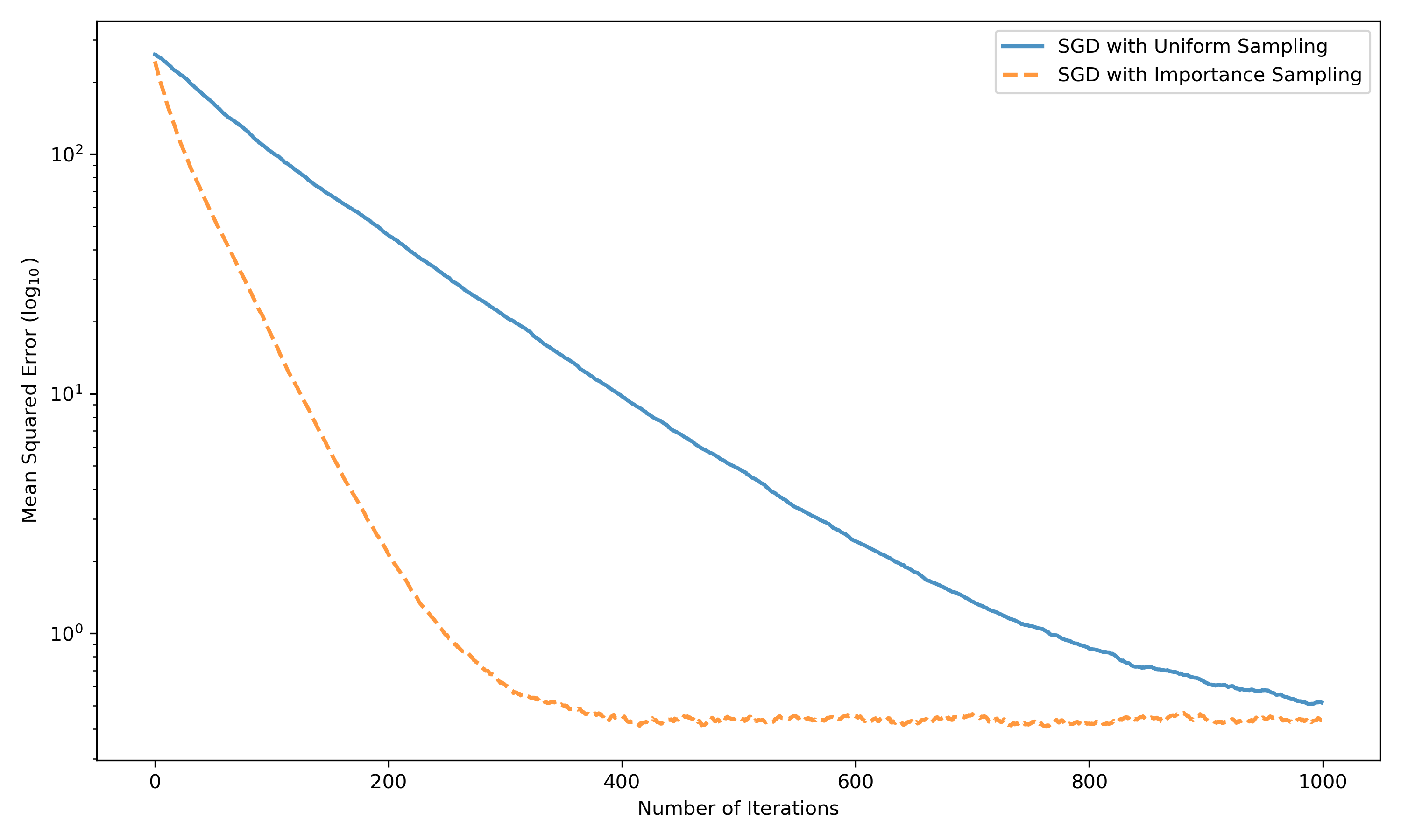
See Figure 1 for an empirical illustration of the speed-up. In fact, only affects the convergence rate through , meaning the maximal increase in exponent always depends on the ratio between and , even for non-binary weighting distributions. The actual gain may, however, be lower. For example, if has rank , then and no speed-up occurs.
As shown in Theorem 3.4(b), the affine operator of Lemma 3.3 describes how the iterates diffuse around their expected path towards . Repeating the argument in (29) without the trace operator leads to the estimate
| (15) |
where the second inequality follows from the assumption on in Theorem 3.4. Rescaling such that , the previous display remains bounded by . This may seem surprising; measures the variance added by the random weighting, so one may expect an increase in to cause a larger long-run variance of the iterates. However, the condition on in Theorem 3.4 automatically regulates the variance level.
This further underlines the importance of designing a weighting scheme that interacts well with the linear regression problem (2), to prevent a “bad” weighted solution . The iterates asymptotically cluster near , so the fit of the latter holds great influence over the long-run statistical properties of the algorithm, as illustrated by the next result.
Theorem 4.1.
Suppose for some true unknown parameter and independent centered measurement noise with covariance matrix . If and satisfies the assumptions of Theorem 3.4(b), then
for any deterministic initialization , where
with expectation taken over both and the sequence of random weighting matrices , .
The result shows that asymptotic recovery of depends almost entirely on the quality of as an estimator of . This may seem unexpected; different weighting distributions yield roughly comparable performance in the asymptotic regime if they feature the same expected weighting matrix , regardless of the actual shape of the distribution. For example, given a probability vector , any binary sampling scheme such that yields similar asymptotic performance since for any such distribution. This includes weighted SGD [needell_srebro_et_al_2014], weighted mini-batch SGD [needell_ward_2017, csiba_richtarik_2018], and independent sampling as in the stochastic Metropolis-Hastings method analyzed in [bieringer_kasieczka_et_al_2023]. Further, gives an example of a heavy-tailed weighting with continuous outcomes for which the iterates will cluster near the same weighted estimator .
Intuitively, this phenomenon appears due to a Gauss-Markov like property of the weighted estimator , in combination with the specific form of the affine operator in Lemma 3.3. By definition, is a deterministic linear transformation of , whereas each iterate results from a random affine transformation of . Theorem 3 of [clara_langer_et_al_2024] then shows that the covariance between and roughly scales with . Convergence in expectation (Lemma 2.1) now implies that the two are asymptotically uncorrelated, so must always have at least as much variance as while featuring the same bias. This yields the lower bound in Theorem 4.1, with the upper bound resulting from an estimate for the additional variance in terms of , analogous to the calculation (15).
The lower bound in Theorem 4.1 represents the fundamental bias-variance trade off in recovering via the weighted least squares estimator , with giving the bias term and the trace expression giving the variance term. One may expect that the bias should read , but this turns out to be equivalent as gives the orthogonal projection onto and . If , the variance term reduces to and matches the risk of the usual linear least squares estimator . The identity only holds under specific conditions, see Lemma D.1(d) for a sufficient one and Theorem 1.4.1 in [campbell_meyer_2009] for a more general result.
In fact, a “bad” expected weighting matrix has the potential to create arbitrarily large lower bounds in Theorem 4.1, as illustrated by the following example. Since for a rank one matrix,
Whenever , the second data point is more informative regarding the value of . If , randomly weighted SGD with and now causes the risk of to blow up in comparison with since
Despite the two data points being linearly dependent, meaning they should in principle contain the same geometric information about , prioritizing training on the “wrong” data point leads to bad statistical performance of the iterates .
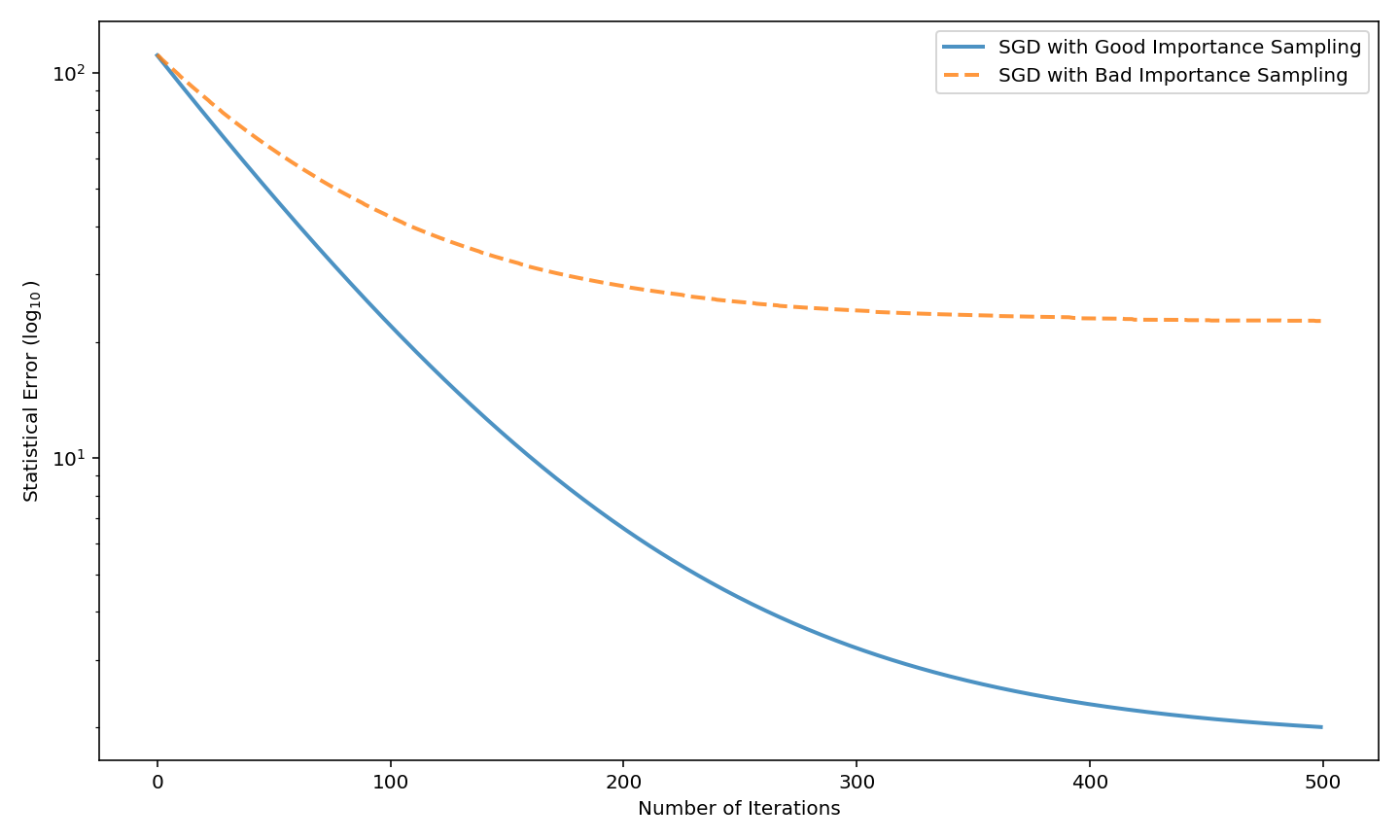
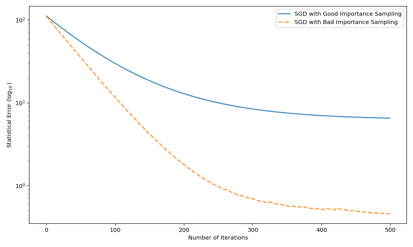
A weighting scheme that favors rows of with larger magnitudes, as introduced in the beginning of this section, naturally avoids the pathology of the previous example. However, the statistical noise may still result in better recovery of despite a “bad” weighting distribution. Suppose again that is diagonal, but not equal to the identity matrix, then the previous calculation in the rank-one setting leads to
If is sufficiently large in comparison with , then iterates prioritizing the less informative data point will outperform a uniform weighting distribution.
This illustrates a point of tension between the goals of fast optimization and statistically optimal estimation. In common statistical usage, the weighted least squares estimator is employed to reduce the variance of estimates based on data points of differing reliability. For uncorrelated statistical noise , this relies on weighting each data point according to an estimate of , see [strutz_2016]. A weighting scheme that prioritizes the wrong data points may accidentally amplify the residual variances, as shown in the example above and in Figure 2 for the randomly weighted iterates. This underlines how choices of optimization hyper-parameters, such as the sampling distribution of data points, can effectively change the underlying statistical estimation problem to cause undesirable outcomes.
5 Discussion and Outlook
We conclude with a discussion of some possible directions for future research. One of the main limitations of our current study lies in the model choice. Linear regression does not encapsulate all the complexities of optimizing the empirical risk of a non-linear deep neural network. In general, a depth network takes the form
with and , a collection of (usually non-linear) activation functions. Training such a network through ERM requires estimating the entries of each affine transformation , which defines a difficult non-convex optimization problem [li_xu_et_al_2018]. As an intermediate step in terms of model complexity, the study of matrix factorizations has experienced recent progress [arora_cohen_et_al_2019a, achour_malgouyres_et_al_2024, chatterji_long_et_al_2022]. In particular, full-batch gradient descent shows implicit bias towards nuclear norm minimal solutions when learning two-layer positive semi-definite factorizations [gunasekar_woodworth_et_al_2017]. Hence, one may conjecture that a weighted nuclear norm minimal estimator plays the same role as the weighted linear least squares estimator does in our analysis. Let and respectively denote the matrices containing the observed data points and the vector-valued labels, then two-layer loss with random weighting takes the form
where denotes the norm of a matrix when treated as a vector. This leads to the interlinked random dynamical systems
Taking the conditional expectation and defining and , one may analyze the underlying gradient descent trajectory of the expected loss via the same technique as in [nguegnang_rauhut_et_al_2024]. In contrast, convergence of the second moment seems more complicated. Due to the factorized structure of the loss, appears squared in the gradient with respect to and vice versa. This causes the second moment of the parameters to evolve differently than the approximately affine dynamical structure shown in Lemma 3.3, see also the corresponding discussion in Section 5 of [clara_langer_et_al_2024]. Further, the stationary distribution of the iterates may not be unique; different valleys in the non-convex loss landscape can trap the iterates with probability depending on the initialization. Consequently, any stationary distribution of the iterates only admits local uniqueness inside the basin of attraction of such a valley.
As a non-linear model with potentially interesting behavior under random weightings, we may consider the weight tied auto-encoder studied in [ghosh_frei_et_al_2025]. Consider the empirical risk
with the rectified linear unit (ReLU) activation. As shown in [ghosh_frei_et_al_2025], mini-batch SGD with a constant step-sizes manages to asymptotically find a global minimum of this loss, but the minimum reached depends on the batch size. Accordingly, one may expect that a weighted version of this result holds for SGD with biased sampling.
In the present article, the random weightings are sampled i.i.d., but in practice it may be desirable to introduce dependency across iterations. As an example, one could recompute the weighting distribution after every iteration to identify data points that are most important to update during the following iteration, which is reminiscent of methods such as saliency guided training [ismail_feizi_et_al_2021] and has applications in adaptive feature decorrelation [fröhlich_durst_et_al_2025]. Suppose we sample the diagonal of from a categorical distribution with weights computed as a function of the past . The resulting iterates do not necessarily minimize an expected loss in the form (6) and we may expect that any stationary distribution reached by the iterates strongly depends on the initialization and outcomes of the random weightings during early iterations. Further, recall from the proof of Lemma 3.2 that the evolution of the second moments of the iterates can be computed via the law of total covariance. Dependency across iterations of the weighting distribution then demands repeated application of said law, which leads to many more terms that must be computed. As a starting point, one may consider the case where the weights only depend on , so that the iterates still evolve as a Markov process. The weighted data points and labels should then be replaced with iteration dependent counterparts, where the weighting is given as a function of the previous iteration. We leave the details to future work.
Appendix A Proofs for Section 2
A.1 Proof of Lemma 2.1
Appendix B Proofs for Section 3
B.1 Proof of Lemma 3.2
Combining the conditional expectations (11) and (12) with the VAR representation (8), independence of the random weighting matrices implies
| (16) |
for every . From here, the proof follows the same steps as the proof of Lemma 2.1. Assumptions 3.1(b) and 3.1(c), as well as Lemma D.1(b) show that , so we may use Lemma D.2 and induction on to show that for all . Lemma D.2 also gives the estimate
with each contained in due to Assumption 3.1(a). Together with Lemma D.3(a), this finishes the proof.
B.2 Proof of Lemma 3.3
Throughout this proof, we write for the second moment of with respect to . For any random vectors and , the law of total covariance yields
| (17) |
Taking and and employing the same arguments that led to (11) and (12) yields
Writing for the covariance with respect to , (17) may then be rewritten as
| (18) |
By definition, both and are constant with respect to the randomness induced via the weighting matrices . Using the VAR representation (8), the conditional covariance then simplifies to
| (19) |
To compute the latter expression, we proceed by proving a short technical lemma.
Lemma B.1.
Let a deterministic vector and a random diagonal matrix of matching dimension be given. Suppose exists for each and write for the covariance matrix of the vector with entries , then
where denotes the element-wise product .
Proof.
Using the definition of the covariance matrix of a random vector,
The entries of the right-hand side matrices satisfy
Subtracting the respective entries now yields the claimed element-wise identity
where the right-hand side equals the -entry of . ∎
We now apply this lemma with , which is independent of when conditioning on , so (19) evaluates to
with the covariance matrix of , as defined in Lemma B.1. Combining this computation with (18) and exchanging the expectation with the linear operator now results in the recursion
| (20) |
Symmetry of and the inclusion follow directly from the previous display, so it remains to estimate the norm of this remainder term. To this end, sub-multiplicativity of the spectral norm and Lemma D.3(c) yield
To complete the proof, we may now apply Lemma D.3(b) and Lemma 3.2 to estimate
B.3 Proof of Theorem 3.4
As in the proof of Lemma 3.3, we write . The sequence of second moments satisfies , with the remainder term as computed in (20) vanishing as . Using induction on , we start by proving that
| (21) |
with the convention that the empty composition gives the identity operator. By definition, each is a linear operator for every and so equals , proving the base case. Suppose the result holds up to some , then Lemma 3.3 and linearity of imply
This proves the induction step and so (21) holds for all . To proceed, we require a bound on the effective operator norms of the linear operators when applied to and .
Lemma B.2.
Fix a symmetric -matrix with and
then
Proof.
As is symmetric and maps the space of symmetric matrices to itself, the singular values of are the magnitudes of its eigenvalues. To bound the latter, we will use the variational characterization of the eigenvalues, see Theorem 4.2.6 in [horn_johnson_2013]. Fix a non-zero unit vector . The definition of entails
| (22) |
If , then also , so acts as the identity on . Together with the assumption , this reduces (22) to
| (23) |
so all non-zero eigenvalues of must correspond to eigenvectors in the orthogonal complement of . As is symmetric, it admits a singular value decomposition of the form , with a positive semi-definite -diagonal matrix. Accordingly, for any matrix the Cauchy-Schwarz inequality implies
| (24) |
Applying a similar argument to the singular value decomposition of the symmetric matrix , we also find that
Suppose now that , which implies by Assumption 3.1(c). Taking the absolute value in (22), inserting the previous computations, as well as applying Lemma D.1(c) and Lemma D.3(c), we arrive at the estimate
where we recall that the norm of evaluates to . It now suffices to further bound the scalar multiplying in the previous display, then the variational characterization of eigenvalues completes the proof. Expanding the square and using the assumption on yields the desired inequality
∎
We now return to the expression (21) for , where we will use Lemma B.2 to bound the norm of each constituent summand, which then yields an expression for up to a vanishing remainder.
Lemma B.3.
Proof.
As shown in (23), each linear operator maps the space of matrices satisfying to itself. Due to Assumption 3.1(b) and Lemma 3.3, this includes as well as each remainder term . In turn, repeated application of Lemma B.2 yields the estimates
valid for every and . Together with the estimate for computed in Lemma 3.3, we may now rearrange (21) and take the norm to find the desired bound
∎
We will first prove the statement regarding square summable step-sizes in Theorem 3.4(a). To this end, recall from Lemma 3.3 that
The kernel of the constant symmetric matrix multiplying contains , so the triangle inequality and repeated application of Lemma B.2 result in
| (25) |
where the second inequality follows from sub-multiplicativity of the norm and Lemma D.3(b) and D.3(c). Defining , the latter expression is proportional to . By construction, for every , so Lemma D.3(a) implies
As , the tail series must vanish due to being square summable. The exponential term must then also go to since the are non-summable. Accordingly, (25) converges to , which proves the statement about square-summable step-sizes.
Suppose now that for some constant , then for every . In particular, converges to the Euler-Mascheroni constant from below. Consequently, Lemma D.3(a) implies
where the last inequality follows from. Recall that converges to a finite constant for all , namely , with the latter denoting the Riemann -function. Together with (25), we now arrive at the estimate
Combining the latter with Lemma B.3 and applying Lemma D.3(a) now leads to the desired convergence rate
with constant
This concludes the proof of Theorem 3.4(a).
We now turn our attention to the setting of constant step-sizes , as in Theorem 3.4(b). In this case, the affine map in Lemma 3.3 is the same for each iteration and so Lemma B.3 implies
Recall from Lemma 3.3 that is a symmetric matrix, the kernel of which contains . The collection of matrices with these properties is stable with respect to the usual vector space operations and hence forms a complete metric space under the spectral norm. As shown in Lemma B.2, the effective operator norm of on this space is given by . Consequently, the restriction of to this sub-space may be inverted via its Neumann series (Proposition 5.3.4 in [helemskii_2006], which yields
Combining these computations now leads to the desired convergence rate
with constant
Applying Lemma D.3(a) completes the proof of Theorem 3.4(b).
B.4 Proof of Theorem 3.6
The proof of the first statement follows along similar lines as the proof of Lemma 1 in [li_schmidt-hieber_et_al_2024]. Due to Assumption 3.5(a), both and admit deterministic upper-bounds that are polynomial in , , and , with degree depending on . Consequently, has finite expectation with respect to for all .
Fix , then the specific form of the gradient descent recursion (8) and the coupling between and imply
| (26) |
Due to Assumption 3.1(a), the initial difference is almost surely orthogonal to . For any and ,
so induction on proves that almost surely for all . Taking the expectation with respect to in (26), we may divide and multiply the latter by to rewrite
Write for the unit vector in the direction of , then the conditional expectation of is a deterministic function of . To maximize it, we may take the supremum over the orthogonal complement of . Since is generated independent of and , this results in
To prove the first claim, it now suffices to show that the supremum over in the previous display always leads to a multiplier contained in . By Assumption 3.5(b), the singular values of lie in , meaning . We first treat the case , which allows for the upper bound
Having reduced the problem to bounding the expectation of the squared norm, we further note via symmetry of that
Assumption 3.5(a) and sub-multiplicativity of the norm imply , so an argument similar to (24) yields
Expanding the square of and combining Assumptions 3.5(a) and 3.5(b) with Lemma D.2 now leads to the final bound
| (27) |
Assumption 3.5(b) further implies . The singular values of are always bounded by , so (27) lies strictly below . The case now follows from Hölder’s inequality, see the proof of Lemma 1 in [li_schmidt-hieber_et_al_2024] for more details.
Having verified the GMC property (13) with respect to the algorithmic randomness introduced via the random weightings , we may now integrate over the distributions of and , which proves geometric moment contraction for all such that the initial vectors admit a finite th moment. Applying Corollary 4 of [li_schmidt-hieber_et_al_2024], this proves existence and uniqueness of a stationary distribution for the gradient descent iterates (7). Further, this distribution is independent of the initialization.
To prove the final statement, let denote a random vector following an independent copy of the stationary distribution. Initializing we now perform iterations (7) on and with the same sequence of random weightings. Write for the iterates started from . Due to stationarity, induces the same measure for every , so this yields a coupling of and . Together with the GMC property (13) and the definition of the transportation distance, this implies the convergence rate
with constant implicit in the proof of Theorem 2, [wu_shao_2004]. Taking the th root and applying Lemma D.3(a) now completes the proof.
B.5 Proof of Theorem 3.7
The triangle inequality implies , so the result follows if both right-hand side distances are bounded by . Applying Theorem 3.6, the first distance satisfies
where the second inequality follows from plugging in the assumption on . We may estimate the second distance by bounding the expectation over a particular coupling of and . Choosing the product measure and letting be as defined in (14), this yields the bound
| (28) |
with denoting the expectation over both the random weightings and the initializations. In particular, then matches the conditional expectation . Recall from Theorem 7.12 of [villani_2003] that converging to in implies . By definition, and so continuity of the trace operator implies
Using the limit computed in Theorem 3.4(b), we find the vanishing bound
which leads to the conclusion
As shown in the proof of Theorem 3.4, the inversion of the linear operator on the space of matrices with kernel containing results from the Neumann series . We also recall from Lemma 3.2 that
which is a symmetric matrix with . As shown in (23), the kernel of contains whenever . Hence, we may repeatedly apply Lemma B.2 to find the estimate
| (29) |
Lemma D.1(b) and D.3(c), as well as sub-multiplicativity of the norm imply . Combining these computations into a bound for (28) and taking the square root results in
Due to the assumption on , the latter cannot exceed , which completes the proof.
Appendix C Proofs for Section 4
C.1 Proof of Theorem 4.1
Since and are independent and the only sources of randomness, we may write . The representation (8) of the gradient descent recursion shows that is an affine function of , which in turn also applies to . Consequently, defines a polynomial of order in the components of , with random coefficients that are independent of . The expectations of these coefficients must be uniformly bounded in . Otherwise, the convergent expression (21) in Theorem 3.4(b) would diverge, thereby creating a contradiction. This yields an integrable envelope, so dominated convergence implies
| (30) |
Applying the convergence results in Lemma 3.2 and Theorem 3.4(b), together with the continuous mapping theorem (see Theorem 2.3 of [van_der_vaart_1998]) the latter evaluates to
| (31) |
Due to positive-definiteness, the trace in the previous display cannot be negative, implying the bound . As , this yields the lower bound in Theorem 4.1 via
| (32) |
where since the latter gives the orthogonal projection onto .
The corresponding upper bound follows via analysis of the trace term in (31). Due to the specific form of , as computed in Lemma 3.3, inherits symmetry from . Further, the Schur Product Theorem (see Theorem 5.2.1 of [horn_johnson_1991]) implies the same for positive semi-definiteness. Now, using series expansion to invert , as well as applying Lemma B.2 together with Lemma D.3(d), the trace term satisfies
To further bound the trace in the previous display, note that and define linear operators that satisfy the assumptions of Lemma D.3(d). Consequently, since
where the last inequality follows from the assumption on in Theorem 3.4. As , it suffices to analyze the expected squared norm of . By assumption, and so implies
Together with the computations (31) and (32), this yields the claimed upper bound for the right-hand side of (30).
Appendix D Auxiliary Results
In this appendix we gather the main technical results used in the main text. Due to the nature of the linear regression loss, these tools are predominantly based on classical results in linear algebra.
D.1 Singular Values and Pseudo-Inversion
Let be an -matrix, then any decomposition is a singular value decomposition if the following hold:
-
(a)
The matrix is orthogonal and of size .
-
(b)
The matrix is orthogonal and of size .
-
(c)
The matrix has non-negative diagonal entries, zeroes everywhere else, and is of size .
The diagonal entries of are unique and referred to as the singular values of . Note that for a symmetric square matrix.
We may use the singular value decomposition to invert on the largest possible subspace. The pseudo-inverse of is given by , where denotes the diagonal -matrix with
By construction, and . Both and are diagonal matrices, featuring binary diagonal entries. The singular values of a non-singular matrix are positive, in which case and so .
For more details, we refer to Chapter 17 of [roman_2008]. We collect the relevant properties of the pseudo-inverse in the following lemma.
Lemma D.1.
-
(a)
For any matrix , the identity holds.
-
(b)
For any vector of compatible dimension, .
-
(c)
The minimum norm minimizer of is given by .
-
(d)
Given matrices and of compatible dimensions, whenever has linearly independent columns and has linearly independent rows.
Proof.
-
(a)
Let be a singular value decomposition, then . By construction, and the proof is complete.
-
(b)
Note that , so implies . Since is diagonal, it follows that can only be non-zero when . By definition of , this implies .
-
(c)
See Theorem 17.3 of [roman_2008].
-
(d)
See [greville_1966].
∎
Lastly, we prove a result to estimate the convergence rate of fixed-point iterations in terms of the non-zero singular values of a given matrix.
Lemma D.2.
Fix and suppose . If , then also and
Proof.
Write and let be a singular value decomposition. Permuting the columns of and , we may order the singular values such that if, and only if, . By definition, the column vectors of are orthogonal and in turn
The vector may be expressed as a unique linear combination . Theorem 17.3 of [roman_2008] shows that form an ortho-normal basis for , so implies for all . In turn,
which proves that . Further, the assumption entails for every , so the first diagonal entries of must all lie in . Accordingly, ortho-normality of the implies
To complete the proof, it suffices to note that attains its maximum over at the smallest non-zero diagonal entry of , which coincides with . ∎
D.2 Miscellaneous Facts
We collect various useful results in the following lemma.
Lemma D.3.
-
(a)
Let , be a sequence in , then
for every . In turn, whenever .
-
(b)
For any vectors and ,
-
(c)
Denote by the element-wise product of matrices, then
-
(d)
For any symmetric positive semi-definite matrix and linear operator that maps the space of such matrices to itself,
Proof.
-
(a)
Note that implies . Consequently,
-
(b)
Given any unit vector of the same dimension as , note that . The inner product is maximized over the unit sphere by taking , which proves the result.
-
(c)
See Theorem 5.5.1 in [horn_johnson_1991].
-
(d)
Let be a singular value decomposition and recall that the trace operator satisfies . If denotes a singular value decomposition of , then the definition of implies , provided the diagonal entries of both matrices are ordered in descending fashion. This completes the proof since
∎