Perturbative limits on axion-SU(2) gauge dynamics during inflation from the energy density of spin-2 particles

Abstract

We investigate the conditions under which the perturbative treatment of the backreaction of spin-2 particles on the dynamics of an axion-SU(2) gauge field system breaks down during cosmic inflation. This condition is based on the ratio of the energy density of spin-2 particles from the SU(2) gauge field to that of the background field. The perturbative treatment breaks down when this ratio exceeds unity. We show that this occurs within a parameter space nearly identical to the strong backreaction regime identified in previous studies. However, in some cases, the ratio exceeds unity even before the system enters the strong backreaction regime. Our results suggest that attempts to study the strong backreaction regime using perturbation theory are necessarily limited. Reliable calculations require non-perturbative treatments, such as three-dimensional lattice simulations.

1 Introduction

A pseudo Nambu-Goldstone boson, such as an ‘axionlike’ field $\chi$, plays a profound role in building models of cosmic inflation [Freese:1990rb]. Rich new phenomenology arises when $\chi$ is coupled to Abelian [Anber:2009ua] and non-Abelian [Maleknejad:2011jw, Adshead:2012kp] gauge fields via the Chern-Simons term, $\chi F\tilde{F}$. In particular, the motion of $\chi$ leads to the copious production of gauge-field particles. These particles can source observable scalar- and tensor-mode fluctuations that are parity-violating and non-Gaussian (see Refs. [Maleknejad:2012fw, Komatsu:2022nvu] for reviews and references therein).

However, the produced particles backreact on the background axion and gauge-field dynamics, which could spoil the successful phenomenology of these models [Anber:2009ua, Barnaby:2011qe, Dimastrogiovanni:2016fuu, Fujita:2017jwq]. For this reason, the strong backreaction regime of the axion-U(1) [Cheng:2015oqa, Notari:2016npn, DallAgata:2019yrr, Domcke:2020zez, Peloso:2022ovc, Gorbar:2021rlt, Durrer:2023rhc, vonEckardstein:2023gwk] and axion-SU(2) [Maleknejad:2018nxz, Ishiwata:2021yne, Iarygina:2023mtj, Dimastrogiovanni:2025snj] models is an active area of research today. A comprehensive review of the former can be found in Ref. [Barbon:2025wjl]. In this paper, we focus on the latter.

All of the aforementioned studies on the backreaction of axion-SU(2) models are based on perturbation theory. Specifically, the gauge field is decomposed into a background and linear perturbations. Then, the backreaction on the background evolution of the $\chi$ and gauge fields is calculated by averaging terms that are quadratic in the linear perturbations. But is this approach valid in the strong backreaction regime? We address this issue by calculating the energy density of spin-2 perturbations of the gauge field and comparing it to the background gauge-field energy density. For perturbation theory to be valid, the former must be smaller than the latter.

Ref. [Dimastrogiovanni:2024lzj] studied perturbativity limits by including spin-2 perturbations at second order (one-loop contributions). By requiring the one-loop contributions to be smaller than the tree-level contributions, they obtained perturbative limits on the viable parameter space of axion-SU(2) gauge field dynamics. In contrast, our approach, which is based on energy density, is conceptually different. If the energy density of spin-2 particles exceeds the background energy density, perturbation theory breaks down at all orders.

Throughout this paper, we take $M_{\rm pl}=(8\pi G)^{-1/2}=1$ and use the Friedmann-Lemaître-Robertson-Walker (FLRW) metric tensor, $g_{\mu\nu}={\rm diag}(-1,a^{2}(t),a^{2}(t),a^{2}(t))$, where $t$ and $a(t)$ are the physical time and the scale factor, respectively. The determinant of the metric tensor is denoted as $g$. In our convention, the Einstein’s field equations are given by $G_{\mu\nu}+T_{\mu\nu}=0$, where $G_{\mu\nu}$ and $T_{\mu\nu}$ are the Einstein tensor and the energy-momentum tensor, respectively.

2 Axion-SU(2) gauge model

2.1 The action and Euler-Lagrange equation

In this paper, we work with the spectator axion-SU(2) gauge field model [Dimastrogiovanni:2016fuu], which is given by the action

$$S=\int d^{4}x\sqrt{-g}\left[\frac{1}{2}R+{\cal L}_{\phi}+{\cal L}_{\chi}+{\cal L}_{A}+{\cal L}_{\rm CS}\right]\,,$$ (2.1)

where $R$ is the Ricci scalar and

$${\cal L}_{\phi} =-\frac{1}{2}g^{\mu\nu}\partial_{\mu}\phi\partial_{\nu}\phi-V_{\phi}(\phi)\,,$$ (2.2)

$${\cal L}_{\chi} =-\frac{1}{2}g^{\mu\nu}\partial_{\mu}\chi\partial_{\nu}\chi-V_{\chi}(\chi)\,,$$ (2.3)

$${\cal L}_{A} =-\frac{1}{4}F^{a}_{\mu\nu}F^{a\,\mu\nu}\,,$$ (2.4)

$${\cal L}_{\rm CS} =-\frac{\lambda}{4f}\chi F^{a}_{\mu\nu}\tilde{F}^{a\,\mu\nu}\,.$$ (2.5)

Here, $\phi$ and $\chi$ are the inflaton and spectator axion fields with potentials $V_{\phi}(\phi)$ and $V_{\chi}(\chi)$, respectively. ${\cal L}_{\rm CS}$ is the Chern-Simons (CS) term, where the axion decay constant and the dimensionless coupling constant are given by $f$ and $\lambda$, respectively. $F_{\mu\nu}^{a}$ ($a=1,2,3$) is the field-strength tensor of the SU(2) gauge field, and we define $\tilde{F}^{a\,\mu\nu}=\epsilon^{\mu\nu\rho\sigma}F^{a}_{\rho\sigma}/(2\sqrt{-g})$ with the Levi-Civita symbol satisfying $\epsilon^{0123}=1$. We define the gauge covariant derivative as $\partial_{\mu}-ig_{A}A_{\mu}^{a}T^{a}$, where $g_{A}$ and $T^{a}$ are the gauge coupling constant and the generator of the SU(2), respectively. Here, we do not distinguish between the upper and lower Latin indices $(a,b,c)$ and the repeated indices are summed regardless of their location. The field strength is given by $F_{\mu\nu}^{a}=\partial_{\mu}A_{\nu}^{a}-\partial_{\nu}A_{\mu}^{a}+g_{A}\epsilon^{abc}A_{\mu}^{b}A_{\nu}^{c}$. Our convention is the same as in Refs. [Maleknejad:2018nxz, Ishiwata:2021yne], while in Ref. [Dimastrogiovanni:2016fuu] the opposite sign convention is used for the Chern–Simons term and the interaction term in the gauge-covariant derivative. They are related to each other via the replacement, $\lambda\to-\lambda$ and $g_{A}\to-g_{A}$.

The Euler-Lagrange equations are

$$\nabla_{\mu}(\partial^{\mu}\phi)-V^{\prime}_{\phi}(\phi)=0\,,$$ (2.6)

$$\nabla_{\mu}(\partial^{\mu}\chi)-V^{\prime}_{\chi}(\chi)-\frac{\lambda}{4f}F^{a}_{\mu\nu}\tilde{F}^{a\,\mu\nu}=0\,,$$ (2.7)

$$\left[D_{\mu}{\cal F}^{\mu\nu}\right]^{a}\equiv\nabla_{\mu}{\cal F}^{a\,\mu\nu}-ig_{A}(T^{b})_{ac}A^{b}_{\mu}{\cal F}^{c\,\mu\nu}=0\,,$$ (2.8)

where $\nabla_{\mu}$ is the covariant derivative, $V^{\prime}_{\phi}(\phi)=\derivative*{V_{\phi}}{\phi}$, $V^{\prime}_{\chi}(\chi)=\derivative*{V_{\chi}}{\chi}$, and ${\cal F}^{a\,\mu\nu}\equiv F^{a\,\mu\nu}+\frac{\lambda}{f}\chi\tilde{F}^{a\,\mu\nu}$. $i(T^{b})_{ac}=\epsilon^{bac}$ is used for the adjoint representation.

The total energy momentum tensor, $T_{\mu\nu}=T^{\phi}_{\mu\nu}+T^{\chi}_{\mu\nu}+T^{A}_{\mu\nu}$, is conserved:

$$\nabla_{\mu}T^{\mu}_{~\nu}=\frac{1}{\sqrt{-g}}\partial_{\mu}(\sqrt{-g}T^{\mu}_{~\nu})-\frac{1}{2}\partial_{\nu}g_{\alpha\beta}T^{\alpha\beta}=0\,,$$ (2.9)

where

$$T^{\phi}_{\mu\nu} =-\partial_{\mu}\phi\partial_{\nu}\phi-g_{\mu\nu}{\cal L}_{\phi}\,,$$ (2.10)

$$T^{\chi}_{\mu\nu} =-\partial_{\mu}\chi\partial_{\nu}\chi-g_{\mu\nu}{\cal L}_{\chi}\,,$$ (2.11)

$$T^{A}_{\mu\nu} =-F^{a}_{\mu\alpha}F^{a\,\alpha}_{\nu}-g_{\mu\nu}{\cal L}_{A}\,.$$ (2.12)

Since the inflaton sector is decoupled, $\nabla_{\mu}T^{\phi\mu}_{~~\nu}=0$ holds. The energy density of the inflaton, axion, and gauge fields are respectively given by $\rho_{X}=T^{X0}_{~~~0}$ ($X=\phi,\chi,A$) and evaluated in Appendix A. The Hubble parameter is given by $H^{2}=\sum_{X}\rho_{X}/3$.

2.2 Spectator axion and gauge fields

In our study, $\rho_{\phi}$ dominates the total energy density during inflation,

$$\rho_{\phi}\gg\rho_{\chi},\,\rho_{A}\,,~~-\dot{H}/H^{2}\ll 1\,,$$ (2.13)

where dots denote time derivatives. Hereafter we will disregard the inhomogeneity in the inflaton and axion fields. Namely, we take

$$\phi=\phi(t)\,,~~~\chi=\chi(t)\,.$$ (2.14)

Then, the time derivative of $H$ is given by

$$-\frac{\dot{H}}{H^{2}}=\frac{\dot{\phi}^{2}}{2H^{2}}+\frac{\dot{\chi}^{2}}{2H^{2}}+\frac{2\rho_{A}}{3H^{2}}\,.$$ (2.15)

We will use this expression to check that $-\dot{H}/H^{2}\ll 1$ is satisfied. In what follows, we will neglect this term unless stated otherwise.

Unlike in Refs. [Dimastrogiovanni:2024xvc, Dimastrogiovanni:2025snj], Eq. (2.15) does not contain the backreaction term, ${\cal J}_{A}$. The time derivative of $H$ is given by the sum of the energy density, $\rho_{X}$, and pressure, $P_{X}$, of $X=(\phi,\chi,A)$ as $\dot{H}=-\sum_{X}(\rho_{X}+P_{X})/2$. Using $\rho_{\phi}+P_{\phi}=\dot{\phi}^{2}$, $\rho_{\chi}+P_{\chi}=\dot{\chi}^{2}$, and $\rho_{A}+P_{A}=4\rho_{A}/3$, we obtain Eq. (2.15) without invoking the equations of motion and, therefore, without ${\cal J}_{A}$. See Appendix B for more details.

Under this background configuration, $A^{a}_{\mu}$ acquires an isotropic and homogeneous background solution $\bar{A}^{a}_{\mu}$ [Maleknejad:2011jw, Maleknejad:2011sq]:

$$\bar{A}^{a}_{0}=0\,,~~~\bar{A}^{a}_{i}=a(t)Q(t)\delta^{a}_{i}\,.$$ (2.16)

This is an attractor solution [Maleknejad:2013npa, Wolfson:2020fqz, Wolfson:2021fya]. In addition, the perturbation around the background solution, $\delta A^{a}_{i}$, contains scalar, vector, and tensor modes. The tensor mode is especially important and affects the dynamics of the homogeneous solution via backreaction [Dimastrogiovanni:2016fuu, Fujita:2017jwq]. Writing the tensor mode as $\delta A^{a}_{i}=B_{ai}\,(=B_{ia})$, and plugging Eq. (2.14) and

$$A^{a}_{0}=0\,,~~~A^{a}_{i}=\bar{A}^{a}_{i}+\delta A^{a}_{i}\,,$$ (2.17)

into Eqs. (2.6) and (2.7), we get

$$\ddot{\phi}+3H\dot{\phi}+V^{\prime}_{\phi}(\phi)=0\,,$$ (2.18)

$$\ddot{\chi}+3H\dot{\chi}+V^{\prime}_{\chi}(\chi)+\frac{3g_{A}\lambda}{fa^{3}}(aQ)^{2}\partial_{t}(aQ)-{\cal P}_{\chi}=0\,,$$ (2.19)

$$\frac{\partial_{t}^{2}(aQ)}{a}+\frac{H\partial_{t}(aQ)}{a}+2g_{A}^{2}Q^{3}-\frac{g_{A}\lambda}{f}\dot{\chi}Q^{2}+{\cal J}_{A}=0\,.$$ (2.20)

Here, we use the FLRW metric, and $\partial_{t}=\partial/\partial t$. For simplicity, the $t$ dependence of the fields and the scale factor is omitted. Eq. (2.20) is obtained from the $\nu=i$ component of Eq. (2.8) contracted with $\delta^{a}_{i}$. Hereafter we will ignore the dynamics of $\phi$, since it does not affect the other fields.

${\cal P}_{\chi}$ and ${\cal J}_{A}$ are the contributions from the perturbation at ${\cal O}(B_{ij}^{2})$ [Maleknejad:2018nxz, Ishiwata:2021yne],

$${\cal P}_{\chi} =\frac{\lambda}{2fa^{3}}\left[2\epsilon^{iqp}\partial_{i}B_{pj}\dot{B}_{qj}+\partial_{t}(g_{A}aQB_{ij}^{2})\right]\,,$$ (2.21)

$${\cal J}_{A} =\frac{g_{A}}{3a^{2}}\left[\frac{1}{a}\epsilon^{iqp}\partial_{i}B_{jp}B_{jq}+\frac{\lambda}{2f}\dot{\chi}B_{ij}^{2}\right]\,,$$ (2.22)

where the Latin indices are 1,2,3 and the Levi-Civita symbol satisfies $\epsilon^{123}=1$. We do not distinguish between upper and lower indices and repeated indices are summed regardless of their location. We omit the symbol of the vacuum expectation value $\expectationvalue{\cdots}$ on the right-hand side for notational simplicity.

We write the symmetric tensor, $B_{ij}$, in terms of the helicity eigenstates, $T_{L}$ (left) and $T_{R}$ (right), of the spin-2 fields that are canonically normalized. For $\vec{k}=(0,0,|k|)$, for instance, $T_{L,R}=B_{11}\pm iB_{12}$. The sign $\pm$ corresponds to the left- ($+$) and right-handed ($-$) field. Then, $T_{L,R}$ are mixed with the helicity eigenstates of gravitational waves, $\psi_{L,R}$, i.e., the tensor modes of the metric perturbation. For the same $\vec{k}$, they are related to the metric perturbations of the tensor modes as $\psi_{L,R}=a(h_{+}\pm ih_{\times})/2$, where $\delta g_{11}=a^{2}h_{+}$ and $\delta g_{12}=a^{2}h_{\times}$ .

The linear equations of motion for $T_{L,R}$ and $\psi_{L,R}$ in the wavenumber space are given by ignoring the non-linear terms,

$$\partial^{2}_{\tau}T_{L,R}+\Omega^{2}_{T}T_{L,R}=-2\frac{\delta_{Q1}}{\tau}\partial_{\tau}\psi_{L,R}+\frac{2}{\tau^{2}}\left[\sqrt{\epsilon_{Q_{B}}}(m_{Q}\mp k\tau)-(\delta_{Q1}+\delta_{Q2})\right]\psi_{L,R}\,,$$ (2.23)

$$\partial^{2}_{\tau}\psi_{L,R}+\Omega_{\psi}^{2}\psi_{L,R}=2\frac{\delta_{Q1}}{\tau}\partial_{\tau}T_{L,R}+\frac{2\sqrt{\epsilon_{Q_{B}}}}{\tau^{2}}\left[m_{Q}\mp k\tau\right]T_{L,R}\,,$$ (2.24)

where $\tau=\int dt/a(t)=-1/(aH)$ is the conformal time and

$$\Omega_{T}^{2}=k^{2}+\frac{2}{\tau^{2}}\left\{m_{Q}\xi\mp k\tau(m_{Q}+\xi)\right\}\,,~~\Omega_{\psi}^{2}=k^{2}-\frac{2}{\tau^{2}}\,,$$ (2.25)

$$m_{Q}=\frac{g_{A}Q}{H}\,,~~\xi=\frac{\lambda\dot{\chi}}{2fH}\,,~~{\cal Q}\equiv aQ\,,$$ (2.26)

$$\delta_{Q1}=H\tau^{2}\partial_{\tau}{\cal Q}\,,~~\delta_{Q2}=H\tau^{3}\partial^{2}_{\tau}{\cal Q}\,,~~\epsilon_{Q_{E}}=\frac{(\dot{Q}+HQ)^{2}}{H^{2}}\,,~~\epsilon_{Q_{B}}=\frac{g_{A}^{2}Q^{4}}{H^{2}}\,.$$ (2.27)

Throughout this paper, we use the same notation, $T_{L,R}$ and $\psi_{L,R}$, for the coordinate-space and momentum-space representations. In Eqs. (2.23) and (2.24), the sign $\mp$ corresponds to “L” and “R” of the subscript.

In the above equations, $\delta_{Q1}$ and $\delta_{Q2}$ are new variables, which have not appeared in previous studies. By rewriting them as

$$\delta_{Q1}=\frac{\dot{Q}+HQ}{H}\,,~~~\delta_{Q2}=-\frac{2QH^{2}+3H\dot{Q}+\ddot{Q}}{H^{2}}\,,$$ (2.28)

they are related to the slow-roll parameter, $\sqrt{\epsilon_{Q_{E}}}$, as

$$\delta_{Q1} =\sqrt{\epsilon_{Q_{E}}}~~~~~~~~{\rm if}~\dot{Q}+HQ>0\,,$$ (2.29)

$$\delta_{Q1}+\delta_{Q2} \simeq-\sqrt{\epsilon_{Q_{E}}}~~~~~~{\rm if}~\dot{Q}\simeq 0~{\rm and}~\ddot{Q}\simeq 0\,.$$ (2.30)

With this approximation, Eqs. (2.23) and (2.24) agree with those in the literature (e.g., Ref. [Dimastrogiovanni:2016fuu]). In this paper, we solve the differential equations given in Eqs. (2.23) and (2.24) without this approximation.

The energy density of the gauge field at ${\cal O}(B_{ij}^{2})$ is given by $\rho_{A}=\bar{\rho}_{A}+\delta\rho_{A}$, where

$$\bar{\rho}_{A} =\frac{3}{2}H^{2}(\epsilon_{Q_{E}}+\epsilon_{Q_{B}})\,,$$ (2.31)

$$\delta\rho_{A} =\frac{1}{2a^{2}}\left[\dot{B}_{ij}^{2}-\frac{1}{a^{2}}B_{ij}\nabla^{2}B_{ij}+\frac{2g_{A}Q}{a}\epsilon^{iqp}B_{jq}\partial_{i}B_{jp}\right]\,.$$ (2.32)

The derivation is given in Eqs. (A.6) and (A.7) in Appendix A. When $\delta\rho_{A}>\bar{\rho}_{A}$, the gauge-field sector becomes non-perturbative due to self-interaction. The background-perturbation split is no longer valid and $B_{ij}$ cannot be treated as a perturbation. Therefore, we cannot write the equations of motion for $Q$ and $B_{ij}$ separately, as in Eqs. (2.20) and (2.23), because higher-order terms in $B_{ij}$ due to self-interaction cannot be ignored. For this reason, we use the threshold, $|\delta\rho_{A}|/\bar{\rho}_{A}=1$, to define the perturbative limit.

Our criterion for the perturbative limit does not apply to axion-U(1) models. The equations of motion for the U(1) gauge field do not contain non-linear terms when the axion is homogeneous due to the absence of self-interaction. The perturbative limit of the axion-U(1) system comes from the interaction between the inhomogeneous axion and gauge fields [Ferreira:2015omg], which is not captured in our work.

Using the mode functions, $T_{h}$, we write ${\cal P}_{\chi}$ [Eq. (2.21)], ${\cal J}_{A}$ [Eq. (2.22)], and $\delta\rho_{A}$ in terms of the wavenumber integral,

$${\cal P}_{\chi} =\frac{\lambda}{2fa^{3}}\partialderivative{t}\sum_{h=L,R}\int\frac{d^{3}k}{(2\pi)^{3}}\left[c_{h}k+aHm_{Q}\right]|T_{h}|^{2}$$ (2.33)

$${\cal J}_{A} =\frac{g_{A}}{3a^{3}}\sum_{h=L,R}\int\frac{d^{3}k}{(2\pi)^{3}}\left[c_{h}k+aH\xi\right]|T_{h}|^{2}\,,$$ (2.34)

$$\delta\rho_{A} =\frac{1}{2a^{2}}\sum_{h=L,R}\int\frac{d^{3}k}{(2\pi)^{3}}\left[|\dot{T}_{h}|^{2}+\left(\frac{k^{2}}{a^{2}}+2m_{Q}H\frac{c_{h}k}{a}\right)|T_{h}|^{2}\right]\,,$$ (2.35)

where $c_{h}=1\,(-1)$ for the left (right)-handed field.

3 Numerical method

We solve the integro-differential equation using ODE solvers provided in Julia [Bezanson:2014pyv]. We introduce $y=-\ln(-\tau)=\ln aH$, which is effectively the number of $e$-folds during inflation, as time coordinates. Using $\derivative*{t}=H\derivative*{y}$ and $\derivative*{\tau}=-\tau^{-1}\derivative*{y}$, the equations of motion for the axion and the background gauge field become

$$\tilde{\chi}^{\prime\prime}+3\tilde{\chi}^{\prime}-\frac{\beta(\chi)}{\lambda}=-\frac{3}{\lambda\kappa}m_{Q}^{2}(m_{Q}+m_{Q}^{\prime})+\tilde{{\cal P}}_{\chi}\,,$$ (3.1)

$$m_{Q}^{\prime\prime}+3m^{\prime}_{Q}+2m_{Q}(1+m^{2}_{Q})=\lambda m_{Q}^{2}\tilde{\chi}^{\prime}-\tilde{{\cal J}}_{A}\,,$$ (3.2)

where

$$\tilde{\chi}\equiv\frac{\chi}{f}\,,~~\kappa\equiv\left(\frac{g_{A}f}{\lambda H}\right)^{2}\,,~~\beta(\chi)\equiv-\frac{\lambda V^{\prime}_{\chi}(\chi)}{H^{2}f}\,,~~\tilde{{\cal P}}_{\chi}=\frac{1}{fH^{2}}{\cal P}_{\chi}\,,~~\tilde{{\cal J}}_{A}=\frac{g_{A}}{H^{3}}{\cal J}_{A}\,.$$ (3.3)

Here, the primes denote the derivatives with respect to $y$, unless they act on $V_{\chi}$ and $V_{\phi}$. In our numerical study, we take the potential of the axion as [Freese:1990rb]

$$V_{\chi}=\mu^{4}(1+\cos\tilde{\chi})\,.$$ (3.4)

Similarly, the linear equations of motion for the tensor modes are

$$T^{\prime\prime}_{L,R}+T^{\prime}_{L,R}+\tau^{2}\Omega_{T}^{2}T_{L,R}=2\delta_{Q1}\psi^{\prime}_{L,R}+2\left[\sqrt{\epsilon_{Q_{B}}}(m_{Q}\mp k\tau)-(\delta_{Q1}+\delta_{Q2})\right]\psi_{L,R}\,,$$ (3.5)

$$\psi^{\prime\prime}_{L,R}+\psi^{\prime}_{L,R}+\tau^{2}\Omega_{\psi}^{2}\psi_{L,R}=-2\delta_{Q1}T^{\prime}_{L,R}+2\sqrt{\epsilon_{Q_{B}}}\left[m_{Q}\mp k\tau\right]T_{L,R}\,,$$ (3.6)

where $\tau=-e^{-y}$, $\delta_{Q1}=H(m_{Q}+m^{\prime}_{Q})/g_{A}$, and $\delta_{Q2}=-H(m_{Q}^{\prime\prime}+3m_{Q}^{\prime}+2m_{Q})/g_{A}$.

We adopt the method given in Ref. [Fujita:2018ndp], in which the tensor modes are decomposed into intrinsic and sourced perturbations. See Appendix C for details. We numerically solve Eqs. (3.1), (3.2), (3.5), and (3.6) in the range $y=[0,25]$. Eqs. (3.5) and (3.6) are solved for each wavenumber $k$ and integrated to obtain $\tilde{{\cal P}}_{\chi}$, $\tilde{J}_{A}$, and $\delta\rho_{A}$ using Eqs. (2.33), (2.34), and (2.35), respectively. The wavenumber space is $k=[10^{-3},10^{12}]$ in units of $aH$ at $y=0$, but we set a cutoff wavenumber $k_{\rm cut}$ to regularize the integrals as follows. The integrands include the contribution of the Bunch-Davies vacuum, which diverges at high $k$. This should be excluded from the integral, since we are calculating the backreaction mainly due to the instability of $T_{R,L}$ caused by the dynamics of the background. To this end, we regularize the integral with a momentum cutoff. The momentum cutoff is given by one of the roots of $\Omega_{T}^{2}=0$ [Maleknejad:2018nxz],

$$k_{\rm cut}=aH\left[|m_{Q}+\xi|+\sqrt{m_{Q}^{2}+\xi^{2}}\right]\,.$$ (3.7)

Here, $aH=e^{y}$, $m_{Q}$ and $\xi$ depend on $y$ and we put the wavenumber upper bound at each $y$ in the integral. This regularization scheme properly accounts for the backreaction. See Appendix D for more details.

The system has five parameters, $\lambda$, $g_{A}$, $\mu$, $f$, and $H$. To investigate how these parameter affect the dynamics, we utilize the known stationary solutions. When $\tilde{\chi}^{\prime\prime}=m_{Q}^{\prime\prime}=0$ in Eqs. (3.1) and (3.2), then the equations of motion for $\tilde{\chi}$ and $m_{Q}$ are diagonalized as

$$m^{\prime}_{Q} =\frac{\kappa\beta(\chi)m_{Q}^{2}-3m_{Q}^{5}-6\kappa m_{Q}(1+m_{Q}^{2})+\kappa\lambda m_{Q}^{2}\tilde{\cal P}_{\chi}-3\kappa\tilde{\cal J}_{A}}{3(3\kappa+m_{Q}^{4})}\,,$$ (3.8)

$$\tilde{\chi}^{\prime} =\frac{\kappa\beta(\chi)-m_{Q}^{3}+2m_{Q}^{5}+\kappa\lambda\tilde{\cal P}_{\chi}+m_{Q}^{2}\tilde{\cal J}_{A}}{\lambda(3\kappa+m_{Q}^{4})}\,.$$ (3.9)

The stationary solutions, $m_{Q}^{\rm st}$, given by $m_{Q}^{\prime}=0$ without the backreaction terms, can be classified depending on the value of $\kappa$ [Ishiwata:2021yne], i.e.,

$${\rm(a)}~ m_{Q}^{\rm st}\simeq\left[\frac{\kappa\beta(\chi)}{3}\right]^{1/3}\,,$$ (3.10)

$${\rm(b)}~ m_{Q}^{\rm st}\simeq\frac{1}{12}\left[\beta(\chi)+\sqrt{\beta(\chi)^{2}-144}\right]\,,$$ (3.11)

for $\kappa\ll 1$ and $\kappa\gg 1$, respectively. We will refer to them as ‘case (a)’ and ‘case (b)’ in the following discussions. The case (a) and (b) solutions were found in Refs. [Adshead:2012kp] and [Ishiwata:2021yne], respectively.

We use the stationary solutions and $\kappa$ to set the five parameters. However, the dynamics are independent of a parameter $\mu^{4}/H^{2}$ when $\dot{H}$ is neglected. With this knowledge, we take the following four parameters as input:

$$\lambda\,,~~g_{A}\,,~~\kappa\,,~~m_{Q}^{\rm in}\,.$$ (3.12)

Then, using $m_{Q}^{\rm in}=m_{Q}^{\rm st}$ with Eqs. (3.10) and (3.11) for $\kappa<1$ and $\kappa>1$, respectively, and $\tilde{\chi}=0.5\pi$, the remaining parameters are determined.

We set initial conditions for the background field values as $m_{Q}^{\rm in}=m_{Q}^{\rm st}(\tilde{\chi}_{i})$ where $\tilde{\chi}_{i}\equiv\tilde{\chi}(y=0)=0.3\pi$. For the derivative of the field, we consider two different initial conditions:

1. $m^{\prime}_{Q}$ and $\tilde{\chi}^{\prime}$ at $y=0$ are given by Eqs. (3.8) and (3.9) ,

2. $m^{\prime}_{Q}=\tilde{\chi}^{\prime}=0$ at $y=0$ .

We set $\lambda=10^{2}$ and take $\kappa=10^{-2}$ and $10^{-1}$ for case (a), and $\kappa=10$ and $10^{2}$ for case (b).

4 Results

4.1 Criterion for the perturbative limit

Using the numerical method described in the previous section, we solve the integro-differential equations of the system. We focus on the validity of the perturbative expansion of the gauge field. As discussed in Section 2.2, the perturbative calculation is invalid if

$$\bar{\rho}_{A}<\delta\rho_{A}\,,$$ (4.1)

where the dependence on $y$ is implicit. This condition is independent of $H$, as $\delta\rho_{A}/\bar{\rho}_{A}$ is a function of $aH=e^{y}$.

Additionally, we set a criterion for the ‘strong backreaction’ by comparing the backreaction terms to the largest terms in the differential equations given in Eqs. (3.1) and (3.2):

$$\tilde{\cal J}_{A}>2m_{Q}(1+m_{Q}^{2})\,~~{\rm or}~~\tilde{\cal P}_{\chi}>\beta/\lambda\,,$$ (4.2)

where again the dependence on $y$ is implicit. If this condition is satisfied, we call it ‘strong backreaction.’

4.2 Solutions for case (a): $\kappa=0.01$

The top two panels of Figure 1 show the dynamics of the background fields, $m_{Q}$ and $\tilde{\chi}$, for $\lambda=10^{2}$, $\kappa=10^{-2}$, and $g_{A}=10^{-3}$ under initial condition (I). The initial condition (II) yields similar results. We verified the accuracy of the calculation by confirming that Eq. (A.20) was satisfied at the $\order{10^{-2}}$ % level. The different lines correspond to various values of $m_{Q}^{\rm in}$. The calculation for the largest value of $m_{Q}^{\rm in}$ is terminated at around $y\simeq 14$ because the dynamics reach the perturbative limit, i.e., $\delta\rho_{A}>\bar{\rho}_{A}$, as shown in the bottom panel. The growth of $\delta\rho_{A}$ arises from the enhancement of the right-handed tensor mode $T_{R}$, which is caused by its instability.

The middle two panels show the backreaction terms, $\tilde{{\cal J}}_{A}$ and $\tilde{\cal P}_{\chi}$, normalized to demonstrate how the backreaction becomes ‘strong’ according to the criterion given in Eq. (4.2). The backreaction terms become comparable to the largest terms in each differential equation at around $y\simeq 14$, which coincides with the perturbative limit. Namely, the growth of $T_{R}$ enhances both the backreaction terms and $\delta\rho_{A}$, thereby breaking the perturbative expansion of the gauge field.

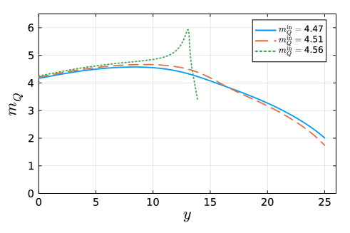
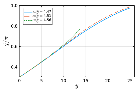
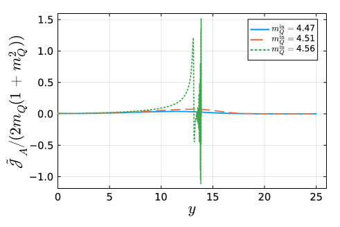
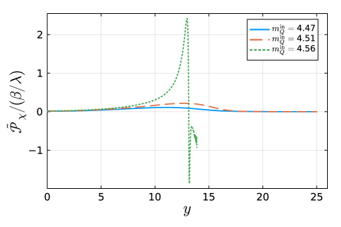
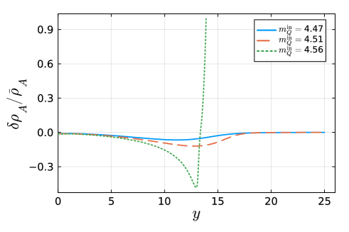
Figure 1: Time evolution of the background fields, $m_{Q}$ (top-left), $\tilde{\chi}$ (top-right), the backreaction term $\tilde{\cal J}_{A}$ divided by $2m_{Q}(1+m^{2}_{Q})$ (middle-left), the backreaction term $\tilde{\cal P}_{\chi}$ divided by $\beta/\lambda$ (middle-right), and $\delta\rho_{A}/\bar{\rho}_{A}$ (bottom), as a function of $y=\ln aH$. The values of the parameters are $\lambda=100$, $\kappa=10^{-2}$, and $g_{A}=10^{-3}$. The input values of $m_{Q}^{\rm in}$ are indicated in the legend. The initial conditions are given by initial condition (I), in which $m_{Q}^{\rm in}=m_{Q}^{\rm st}(\tilde{\chi}=\tilde{\chi}_{i})$, $\tilde{\chi}_{i}=0.3\pi$, and their derivatives are given by Eqs. (3.8) and (3.9).

The slow-roll approximation, $\tilde{\chi}^{\prime\prime}=m^{\prime\prime}_{Q}=\dot{H}=0$ and $\delta_{Q1}=-(\delta_{Q1}+\delta_{Q2})=\sqrt{\epsilon_{Q_{E}}}$, holds for most of the time evolution. The exceptions are the initial oscillatory regime in the early stage and the region near the perturbative limit. Figure 8 in Appendix E shows the time evolution of $m^{\prime}_{Q}$, $\xi$, $\delta_{Q1}$, and $\delta_{Q1}+\delta_{Q2}$. See the discussion there for more details. On the other hand, $-\dot{H}/H^{2}$ is always small. The behavior remains qualitatively unchanged for $\kappa=10^{-1}$ and other values of $g_{A}$. In addition, the choice of initial conditions has little effect on the dynamics. Figure 9 in Appendix E demonstrates this with the results for initial condition (II). In this case, while the amplitudes of the oscillation in $m^{\prime}_{Q}$, $\xi$ and the slow-roll parameters increase, the time evolution of the background fields remains unaffected.

4.3 Solutions for case (b): $\kappa=100$

Figure 2 shows the results for $\kappa=10^{2}$ under initial condition (I). The input values of $m_{Q}^{\rm in}$ are adjusted accordingly. We verified the accuracy of the calculation again by confirming that Eq. (A.20) was satisfied at the $\order{10^{-2}}$ % level. As in case (a), we encountered the perturbative limit and the strong backreaction almost simultaneously. We find that, while $\tilde{\cal J}_{A}$ increases, the contribution of $\tilde{\cal P}_{\chi}$ to the differential equation is negligible. Consequently, the backreaction has little effect on the dynamics of $\tilde{\chi}$, whereas $m_{Q}$ behaves differently depending on $m_{Q}^{\rm in}$.

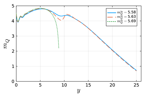
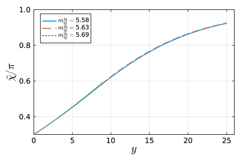
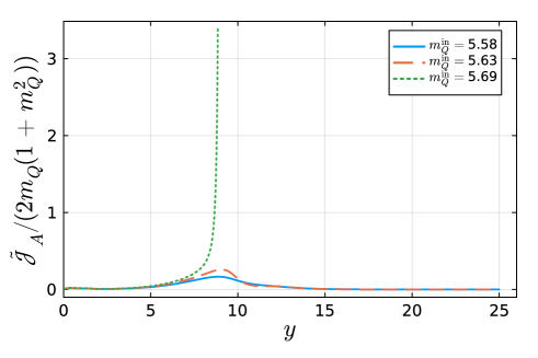
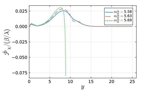
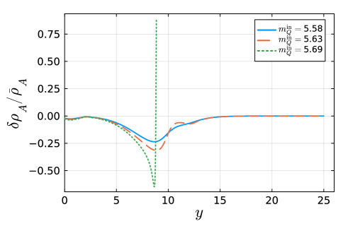
Figure 2: Same as Figure 1, but for $\kappa=10^{2}$.

The slow-roll approximation is less valid than in case (a). The slow-roll result of $m_{Q}^{\prime}$ assuming Eq. (3.8) deviates from the exact numerical solution over a wide range of time evolution. The approximation of $\delta_{Q1}+\delta_{Q2}\simeq-\sqrt{\epsilon_{Q_{E}}}$ is also poorer. See Figure 10 in Appendix E for more details.

The behavior of $m_{Q}$ changes drastically for the initial condition (II). The numerical results are shown in Figure 3. We find that $m_{Q}$ decreases rapidly at the beginning. This is due to the $2m_{Q}(1+m^{2}_{Q})$ term on the left-hand side of Eq. (3.2), which reduces $m_{Q}$. On the other hand, $\tilde{\chi}^{\prime}$ soon becomes positive and the term $\lambda m_{Q}^{2}\tilde{\chi}^{\prime}$ contributes in Eq. (3.2). After that, $m_{Q}$ approaches $m_{Q}^{\rm st}$. The suppression of $m_{Q}$ leads to a smaller value of $\bar{\rho}_{A}$, making the perturbative limit easier to reach. On the other hand, the backreaction terms are small and the system does not enter the strong backreaction regime.

The derivatives of the background field and the slow-roll parameters are presented in Figure 11 in Appendix E, and are qualitatively similar to Figure 10.

Regarding the accuracy of the numerical calculation, we find that, for a brief moment, Eq. (A.20) is violated by $\order{10}\%$. At that moment, both sides of Eq. (A.20) are suppressed, causing the relative deviation between the right- and left-hand sides to increase. However, Eq. (A.20) cannot be used for the check in this case because it is derived by neglecting the right-hand side of the equation of motion for $T_{L/R}$, which is also suppressed by the slow-roll parameters. After passing that point, we find that Eq. (A.20) holds at the $\order{10^{-2}}$% level.

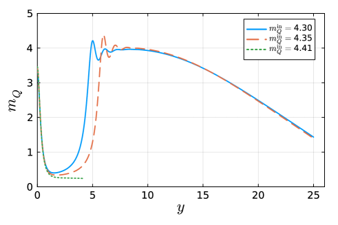
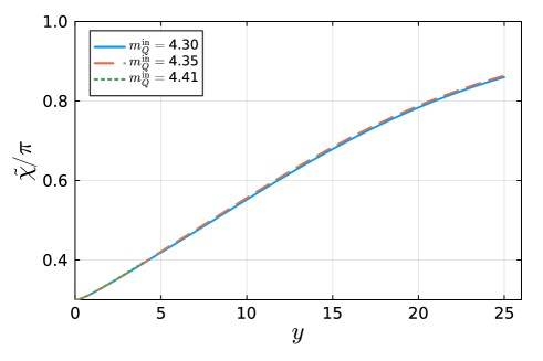
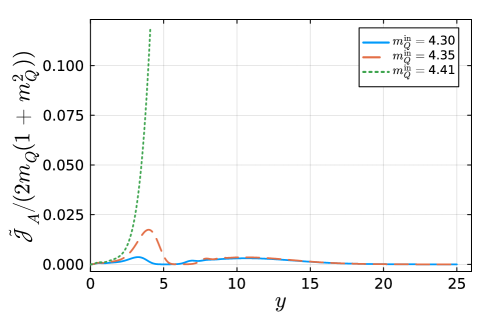
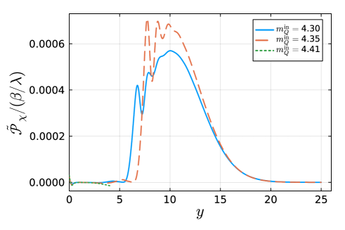
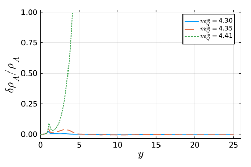
Figure 3: Same as Figure 2, but under initial condition (II), in which the initial conditions for the derivatives of the background fields are given by $m^{\prime}_{Q}=\tilde{\chi}^{\prime}=0$.

4.4 Perturbative limit

Figure 4 shows the perturbative limit for case (a) with $\kappa=10^{-2}$ and $10^{-1}$ under initial condition (I). The initial condition (II) yields similar results. The dashed line shows the stable solution found in Ref. [Ishiwata:2021yne]. Below this line, the backreaction terms have a negligible effect on the solutions, and the slow-roll approximation remains valid. We find that the boundary of the perturbative limit nearly coincides with the bound of the strong backreaction. Therefore, the perturbative calculation breaks down when the backreaction is strong. This is the main conclusion of this paper.

To further investigate the possible dependence on initial conditions, we computed the dynamics using different initial conditions. For instance, a larger value of initial $\tilde{\chi}^{\prime}$, such as $1.5$–$2$ times larger than that given in Eq. (3.9), induces strong backreaction, while perturbativity holds for a certain value of $m_{Q}^{\rm in}$. However, even in this specific case, the perturbative calculation breaks down when $m_{Q}^{\rm in}$ is a few % larger. Therefore, our main conclusion is valid for case (a), irrespective of the initial conditions within the percent-level uncertainty.

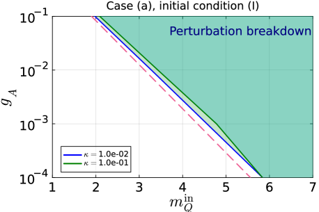
Figure 4: Perturbative limit on the $g_{A}$-$m_{Q}^{\rm in}$ plane for case (a) with $\lambda=10^{2}$ under initial condition (I). The perturbative calculation breaks down, i.e. $\delta\rho_{A}>\bar{\rho}_{A}$, in the shaded regions above the solid lines for $\kappa=10^{-2}$ and $10^{-1}$, as indicated in the legend. The dashed line shows the upper limit of the stable solution found in Ref. [Ishiwata:2021yne]. Below this line, the backreaction terms have a negligible effect on the differential equations.

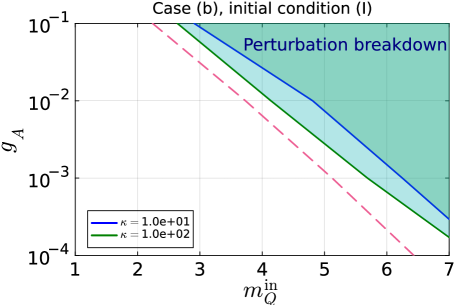
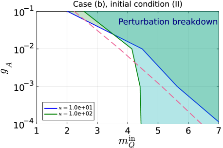
Figure 5: Same as Figure 4, but for case (b) under initial conditions (I) (left) and (II) (right). The shaded regions correspond to the breakdown of the perturbative calculation for $\kappa=10$ and $10^{2}$, as indicated in the legend.

Figure 5 shows the perturbative limit for case (b). Here we show the results under initial conditions (I) (left panel) and (II) (right panel). We also find that the perturbative limit is equivalent to the strong backreaction regime for initial condition (I). This is because the dynamics of case (b) under initial condition (I) are similar to those of case (a), as discussed in Section 4.3.

The situation under initial condition (II) with $\kappa=10$ is similar to that under initial condition (I). On the other hand, the perturbative limit for the case of $\kappa=10^{2}$ is more stringent when $g_{A}\leq 10^{-2}$. This is due to the suppression of $m_{Q}$ in the early stage of the dynamics (see the top left panel of Figure 3), resulting in a smaller value of $\bar{\rho}_{A}$. As a result, the perturbative limit becomes tighter than the strong backreaction. For $g_{A}=10^{-1}$, however, the dynamics are similar to those in Figure 2, and the perturbative limit and the strong backreaction occur similarly to the initial condition (I).

4.5 Gravitational waves

As seen in Eqs. (2.23) and (2.24), the tensor modes of the gauge field, $T_{L,R}$, are linearly mixed with the tensor metric perturbations, $\psi_{L,R}$, which gives rise to the production of primordial gravitational waves [Adshead:2013qp, Dimastrogiovanni:2012ew, Dimastrogiovanni:2016fuu]. The total gravitational wave power spectrum, ${\cal P}_{T}$, is given by ${\cal P}_{T}={\cal P}_{T}^{\rm(vac)}+{\cal P}_{T}^{\rm(src)}$, where

$${\cal P}_{T}^{\rm(vac)} =\lim_{|k\tau|\to 0}\frac{2H^{2}k^{3}\tau^{2}}{\pi^{2}}(|\psi^{\rm int}_{L}|^{2}+|\psi^{\rm int}_{R}|^{2})\simeq\frac{2H^{2}}{\pi^{2}}\,,$$ (4.3)

$${\cal P}_{T}^{\rm(src)} =\lim_{|k\tau|\to 0}\frac{2H^{2}k^{3}\tau^{2}}{\pi^{2}}(|\psi^{\rm src}_{L}|^{2}+|\psi^{\rm src}_{R}|^{2})\,.$$ (4.4)

Here, ${\cal P}_{T}^{\rm(vac)}$ is the vacuum contribution, while ${\cal P}_{T}^{\rm(src)}$ is the sourced contribution from the gauge tensor modes.

The left and right panels of Figure 6 show the power spectra of primordial gravitational waves under initial condition (I) for cases (a) and (b), respectively. The sourced component is dominated by $|\psi_{R}|^{2}$ and is much larger than the vacuum one. We find that the maximum amplitude is $\order{10^{-7}}$ in the perturbative region of case (a). This amplitude is much smaller than the $\order{10^{-3}\,\mathchar 45\relax\,10^{-2}}$ required to explain the recent observation of Pulsar Timing Array (PTA) [NANOGrav:2023gor, EPTA:2023fyk, Reardon:2023gzh, Xu:2023wog], in agreement with Ref. [Unal:2023srk]. However, if we could analyze the strong backreaction of the axion-SU(2) dynamics beyond perturbation theory, the induced gravitational waves might be amplified enough to explain the amplitude of the stochastic gravitational waves reported by the PTA observations.

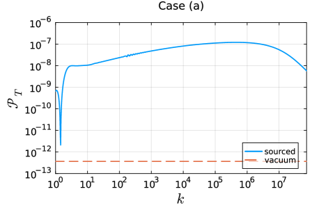
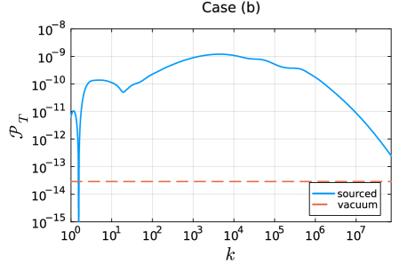
Figure 6: Gravitational waves sourced by the gauge field. (Left) The parameters are the same as in Figure 1 with $m_{Q}^{\rm in}=4.51$. (Right) The parameters are the same as in Figure 2 with $m_{Q}^{\rm in}=5.63$. The dashed lines show the vacuum contributions.

5 Comparison to previous works

Ref. [Dimastrogiovanni:2024lzj] also studied the perturbative limit of the same system as given in Eq. (2.1), focusing on the slow-roll dynamics of case (a). Their approach is based on the comparison between the tree-level and one-loop contributions to the two-point correlation function of the gauge field [Ferreira:2015omg]. In other words, they compared the relative importance of the first- and second-order perturbations in the equations of motion for the gauge field, while all previous work was based on the first-order perturbations. The perturbative limit is reached when the ratio of the one-loop contribution to the tree-level contribution exceeds unity, while in our study the perturbative limit is reached when $\delta\rho_{A}/\bar{\rho}_{A}$ exceeds unity. Their calculations include one-loop contributions from the self-interaction of the gauge fields as well as the non-linear interaction between the inhomogeneous axion and gauge fields. The latter is not addressed in our work, as discussed in Section 2.2. Their conclusion is similar to ours for case (a): the perturbative limit is reached when the system enters the strong reaction regime. In this paper, we have studied case (b) in addition to case (a) and found that the perturbative limit is reached even before the system enters the strong backreaction regime in some cases. Therefore, the perturbative limit depends on the configuration of the background fields of the system and it is not universally determined. It remains to be seen whether their approach yields a similar result for case (b).

On the technical side, we have solved the equations of motion, Eqs. (3.1), (3.2), (3.5), and (3.6), simultaneously without using the slow-roll approximation. In previous studies employing the slow-roll approximation (e.g., [Dimastrogiovanni:2016fuu]), several terms were neglected in the right-hand sides of Eqs. (2.23) and (2.24). In the evaluation of the backreaction terms, we used the cutoff regularization to properly take into account the contribution due to the tachyonic instability of the gauge spin-2 components. Our approach is similar to that of Ref. [Garcia-Bellido:2023ser], in which the backreaction term was analyzed for the axion-U(1) system. Ref. [Iarygina:2023mtj] regularized the integral for case (a) by subtracting the Bunch-Davies-vacuum component from the tensor modes. Their results are consistent with ours.

Refs. [Iarygina:2023mtj] studied the strong backreaction regime of case (a) using perturbation theory. Both our results and those in Ref. [Dimastrogiovanni:2024lzj] suggest that the perturbative approach is invalid in this regime. Therefore, it remains to be seen whether their quantitative results hold under non-linear, non-perturbative calculations.

6 Conclusion

We have investigated the limits of the perturbative treatment of axion-SU(2) gauge field dynamics during inflation. We considered the spectator axion-gauge sector as given in Eq. (2.1) [Dimastrogiovanni:2016fuu]. The system’s field contents include homogeneous axion and gauge fields, as well as the tensor modes (spin-2 perturbations) of the gauge field and the metric tensor. The instability of the tensor modes of the gauge field results in the copious production of spin-2 particles during inflation, which backreacts on the dynamics of the background fields. We find that the energy density of the tensor modes, $\delta\rho_{A}$, grows to be as large as the background gauge field energy density, $\bar{\rho}_{A}$, leading to the breakdown of the perturbative calculation.

The perturbative limits depend on the initial configuration of the background fields. We studied two background configurations, cases (a) [Eq. (3.10)] and (b) [Eq. (3.11)], based on the slow-roll stationary solutions with negligible backreaction. Cases (a) and (b) were found in Refs. [Adshead:2012kp] and [Ishiwata:2021yne], respectively. For each case, we considered two initial conditions, (I) and (II), for the derivatives of the background fields: the slow-roll values and zero, respectively. The dynamics are similar for both initial conditions in case (a), except for the initial oscillatory behavior, and we found similar perturbative limits for both. In contrast, the behavior of the background gauge field changes significantly depending on the initial conditions in case (b). The value of the background gauge field is suppressed under initial condition (II), which reduces its energy density. As a result, the perturbative limit becomes more stringent than in (I).

We studied the correlation between the perturbative limits and the strong backreaction regime, in which the absolute values of the backreaction terms, $\tilde{\cal J}_{A}$ and $\tilde{\cal P}_{\chi}$, become larger than the other dominant terms in the equations of motion. We found that the perturbative limit is reached in the strong backreaction regime, except for certain initial configurations of the background fields. This can be qualitatively understood as follows: the tachyonic instability of the tensor modes enhances $\delta\rho_{A}$ and the backreaction terms almost simultaneously. The exception is case (b) under initial condition (II). In this case, while the backreaction terms are much smaller than the other terms in the equations of motion, $\bar{\rho}_{A}$ is suppressed due to a smaller value of the background gauge field, leading to $\delta\rho_{A}/\bar{\rho}_{A}>1$.

To make progress, we need non-perturbative approaches, such as three-dimensional lattice simulations carried out for axion-U(1) systems [Caravano:2022epk, Figueroa:2023oxc, Figueroa:2024rkr, Sharma:2024nfu, Jamieson:2025ngu], which will help us understand the full dynamics of the axion-SU(2) system during inflation and their observational consequences.

Appendix A Energy momentum tensor

We use the conservation of the energy-momentum tensor to verify the accuracy of the numerical solution of the differential equations. We do not include the metric perturbations in this verification. The result is given in Eq. (A.20).

The energy density is given by

$$\rho_{\chi} =-T^{\chi}_{00}=\frac{\dot{\chi}^{2}}{2}+V_{\chi}\,,$$ (A.1)

$$\rho_{A} =-T^{A}_{00}=\frac{1}{2}a^{-2}(F^{a}_{0i})^{2}+\frac{1}{4}a^{-4}(F^{a}_{ij})^{2}\,,$$ (A.2)

where $T^{\chi}_{\mu\nu}$ and $T^{A}_{\mu\nu}$ are given in Eqs. (2.11) and (2.12), respectively, and

$$(F^{a}_{0i})^{2} =3\dot{{\cal Q}}^{2}+\dot{B}^{2}_{ij}\,,$$ (A.3)

$$(F^{a}_{ij})^{2} =6g_{A}^{2}M^{4}_{Q}-2g_{A}^{2}{\cal Q}^{2}B^{2}_{ij}+(\delta F^{a}_{ij})^{2}\,.$$ (A.4)

We do not distinguish between upper and lower Latin indices ($i,j,a$) and repeated indices are summed regardless of their location. Here, we have introduced ${\cal Q}\equiv aQ$ and

$$(\delta F^{a}_{ij})^{2}=(\partial_{i}B_{jk}-\partial_{j}B_{ik})^{2}+2g_{A}^{2}{\cal Q}^{2}B^{2}_{ij}-4g_{A}{\cal Q}\epsilon^{iqp}(\partial_{i}B_{jq})B_{jp}+\order{B_{ij}^{3}}\,.$$ (A.5)

We will omit the terms of order ${\cal O}(B_{ij}^{3})$ and separate $T^{A}_{00}$ into contributions from the background field and the perturbations:

$$\bar{\rho}_{A} =-T^{A}_{00}|_{\rm BG}=\frac{3}{2}a^{-2}\dot{{\cal Q}}^{2}+\frac{3}{2}a^{-4}g_{A}^{2}{\cal Q}^{4}\,,$$ (A.6)

$$\delta\rho_{A} =-T^{A}_{00}|_{B^{2}}=\frac{1}{2}a^{-2}\dot{B}^{2}_{ij}+\frac{1}{4}a^{-4}\left[(\partial_{i}B_{jk}-\partial_{j}B_{ik})^{2}-4g_{A}{\cal Q}\epsilon^{iqp}(\partial_{i}B_{jq})B_{jp}\right]\,.$$ (A.7)

With $\nabla_{\mu}T^{A\,\mu}_{~~~0}=-a^{-4}\partial_{0}(a^{4}T_{00})+a^{-2}\partial_{i}T_{i0}$ and neglecting the total derivative term, we obtain

$$\nabla_{\mu}T^{\chi\,\mu}_{~~~0}=\dot{\chi}(\ddot{\chi}+3H\dot{\chi}+V^{\prime}_{\chi})\,,$$ (A.8)

$$\nabla_{\mu}T^{A\,\mu}_{~~~\,0}|_{\rm BG}=3\dot{{\cal Q}}a^{-1}\left[a^{-1}\ddot{{\cal Q}}+Ha^{-1}\dot{{\cal Q}}+2g_{A}^{2}Q^{3}\right]\,,$$ (A.9)

$$\nabla_{\mu}T^{A\,\mu}_{~~~\,0}|_{B^{2}}=a^{-5}\partial_{\tau}B_{ij}\left[\partial_{\tau}^{2}B_{ij}-\partial_{i}^{2}B_{ij}+2g_{A}{\cal Q}\epsilon^{kjp}\partial_{k}B_{ip}\right]+a^{-5}g_{A}\partial_{\tau}{\cal Q}\epsilon^{iqp}(\partial_{i}B_{jq})B_{jp}\,.$$ (A.10)

To check the energy conservation, we rewrite the above equations by using the equations of motion. To do so, we need the equation of motion for $B_{ij}$. We derive the Euler-Lagrange equation from the action without metric perturbations. For convenience, we use the conformal time, $\tau$, instead of the physical time, $t$:

$$S|_{B^{2}}=\int d\tau d^{3}x\,a^{4}({\cal L}_{A}+{\cal L}_{\rm CS})|_{B^{2}}\,,$$ (A.11)

where

$$a^{4}{\cal L}_{A}|_{B^{2}} =\frac{1}{2}(\partial_{\tau}B_{ij})^{2}-\frac{1}{4}\left[(\partial_{i}B_{jk}-\partial_{j}B_{ik})^{2}-4g_{A}{\cal Q}\epsilon^{iqp}(\partial_{i}B_{jq})B_{jp}\right]\,,$$ (A.12)

$$a^{4}{\cal L}_{\rm CS}|_{B^{2}} =-\frac{\lambda\chi}{2f}\left[-g_{A}(\partial_{\tau}{\cal Q})B^{2}_{ij}+2(\partial_{\tau}B_{ka})\epsilon^{ijk}\partial_{i}B_{ja}-2g_{A}{\cal Q}(\partial_{\tau}B_{ij})B_{ij}\right]\,.$$ (A.13)

Then, the Euler-Lagrange equation is

$$(\partial_{\tau}^{2}-\partial_{i}^{2})B_{ij}+2g_{A}{\cal Q}\epsilon^{kjp}\partial_{k}B_{ip}+\frac{\lambda\partial_{\tau}\chi}{f}(\epsilon^{kip}\partial_{k}B_{jp}+g_{A}{\cal Q}B_{ij})=0\,.$$ (A.14)

Using the equations of motion, i.e., Eqs. (2.19), (2.20), and (A.14), we find

$$\nabla_{\mu}T^{\chi\,\mu}_{~~~0}=\dot{\chi}\left[-3a^{-1}\frac{g_{A}\lambda}{f}Q^{2}\dot{\cal Q}+{\cal P}_{\chi}\right]\,,$$ (A.15)

$$\nabla_{\mu}T^{A\,\mu}_{~~~\,0}|_{\rm BG}=3\dot{{\cal Q}}a^{-1}\left[\frac{g_{A}\lambda}{f}\dot{\chi}Q^{2}-{\cal J}_{A}\right]\,,$$ (A.16)

$$\nabla_{\mu}T^{A\,\mu}_{~~~\,0}|_{B^{2}}=-\dot{\chi}{\cal P}_{\chi}+3a^{-1}\dot{{\cal Q}}{\cal J}_{A}\,,$$ (A.17)

which leads to the conservation of the total energy-momentum tensor:

$$\nabla_{\mu}T^{\chi\,\mu}_{~~~0}+\nabla_{\mu}T^{A\,\mu}_{~~~\,0}|_{\rm BG}+\nabla_{\mu}T^{A\,\mu}_{~~~\,0}|_{B^{2}}=0\,.$$ (A.18)

We use Eq. (A.16) to verify the accuracy of the numerical solution. We rewrite it using $y=-\ln(-\tau)=\ln aH$ as the time variable:

$$\frac{3}{2}H^{3}a^{-4}\derivative{y}\left[a^{4}(\epsilon_{Q_{E}}+\epsilon_{Q_{B}})\right]=3H^{3}\sqrt{\epsilon_{Q_{E}}}\left[\lambda\sqrt{\epsilon_{Q_{B}}}\tilde{\chi}^{\prime}-\frac{H}{g_{A}}\tilde{{\cal J}}_{A}\right]\,,$$ (A.19)

where $\epsilon_{Q_{E}}$ and $\epsilon_{Q_{B}}$ are defined in Eq. (2.27) and $\tilde{\cal J}$ is defined in Eq. (3.3). Integrating both sides, we get

$$\frac{1}{2}(\epsilon_{Q_{E}}+\epsilon_{Q_{B}})(y)-\frac{1}{2}(\epsilon_{Q_{E}}+\epsilon_{Q_{B}})(0)\frac{a^{4}(0)}{a^{4}(y)}=\frac{1}{a^{4}(y)}\int_{0}^{y}dy^{\prime}\left[\sqrt{\epsilon_{Q_{B}}}\tilde{\chi}-\frac{H}{g_{A}}\tilde{{\cal J}}_{A}\right]\,.$$ (A.20)

We verify the accuracy of our numerical solution by computing both sides of Eq. (A.20) at each step of $y$.

Appendix B Time derivative of the Hubble parameter

The time derivative of the Hubble parameter is given by

$$\dot{H}=-\frac{1}{2}(\rho+P)\,,$$ (B.1)

where $\rho=\rho_{\phi}+\rho_{\chi}+\rho_{A}$ is the total energy density and $P=P_{\phi}+P_{\chi}+P_{A}$ is the total pressure. Using

$$\rho_{\phi}=\frac{\dot{\phi}^{2}}{2}+V_{\phi}\,,~~P_{\phi}=\frac{\dot{\phi}^{2}}{2}-V_{\phi}\,,$$ (B.2)

$$\rho_{\chi}=\frac{\dot{\chi}^{2}}{2}+V_{\chi}\,,~~P_{\chi}=\frac{\dot{\chi}^{2}}{2}-V_{\chi}\,,$$ (B.3)

$$\rho_{A}=3P_{A}\,,$$ (B.4)

we obtain Eq. (2.15).

However, this result does not agree with that given in Refs. [Dimastrogiovanni:2024xvc, Dimastrogiovanni:2025snj], where $\dot{H}$ includes ${\cal J}_{A}$. Therefore, we rederive Eq. (2.15) by taking the derivative of both sides of $3H^{2}=\rho_{\phi}+\rho_{\chi}+\rho_{A}$,

$$\dot{H}=\frac{1}{6H}(\dot{\rho}_{\phi}+\dot{\rho}_{\chi}+\dot{\rho}_{A})\,,$$ (B.5)

and show that the backreaction terms cancel in the final result.

Using the equation of motion, $\dot{\rho}_{\phi}$ and $\dot{\rho}_{\chi}$ are given by

$$\dot{\rho}_{\phi} =-3H\dot{\phi}^{2}\,,$$ (B.6)

$$\dot{\rho}_{\chi} =-3H\dot{\chi}^{2}+\dot{\chi}\left[-3a^{-1}\frac{g_{A}\lambda}{f}Q^{2}\dot{\cal Q}+{\cal P}_{\chi}\right]\,.$$ (B.7)

Using $\nabla_{\mu}T^{A\,\mu}_{~~~0}=-a^{-4}\partial_{0}(a^{4}T_{00})+a^{-2}\partial_{i}T_{i0}$ and Eqs. (A.16) and (A.17), $\dot{\rho}_{A}$ is given by

$$\dot{\rho}_{A}=-4H\rho_{A}+\dot{\chi}\left[3a^{-1}\frac{g_{A}\lambda}{f}Q^{2}\dot{\cal Q}-{\cal P}_{\chi}\right]\,.$$ (B.8)

Combining all of the above, the backreaction terms cancel, and the derivative of the Hubble parameter is obtained as

$$\dot{H}=-\left[\frac{1}{2}\dot{\phi}^{2}+\frac{1}{2}\dot{\chi}^{2}+\frac{2}{3}\rho_{A}\right]\,,$$ (B.9)

where $\rho_{A}=\bar{\rho}_{A}+\delta\rho_{A}$, in agreement with Eq. (2.15).

In terms of the slow-roll parameters, it is given by

$$-\frac{\dot{H}}{H^{2}} =\frac{\dot{\phi}^{2}}{2H^{2}}+\frac{\dot{\chi}^{2}}{2H^{2}}+\frac{2}{3H^{2}}\rho_{A}$$

$$=\epsilon_{\phi}+\epsilon_{\chi}+\epsilon_{Q_{E}}+\epsilon_{Q_{B}}+\frac{2}{3H^{2}}\delta\rho_{A}\,,$$ (B.10)

where $\delta\rho_{A}$, given in Eq. (A.7), is calculated from the tensor perturbations as [Eq. (2.35)]

$$\delta\rho_{A}=\frac{1}{2a^{2}}\sum_{h=L,R}\int\frac{d^{3}k}{(2\pi)^{3}}\left[|\dot{T}_{h}|^{2}+\left(\frac{k^{2}}{a^{2}}+2m_{Q}H\frac{c_{h}k}{a}\right)|T_{h}|^{2}\right]\,.$$ (B.11)

Appendix C Initial conditions for tensor modes

To solve the differential equations of the tensor modes, i.e., Eqs. (3.5) and (3.6), we adopt the procedure shown in Ref. [Fujita:2018ndp]. Considering the tensor field as a linear combination of intrinsic and sourced components, the equations can be decomposed as

$$T^{{\rm int}\,\prime\prime}_{L,R}+T^{{\rm int}\,\prime}_{L,R}+\tau^{2}\Omega_{T}^{2}T^{{\rm int}}_{L,R}=2\delta_{Q1}\psi^{{\rm src}\,\prime}_{L,R}+2\left[\sqrt{\epsilon_{Q_{B}}}(m_{Q}\mp k\tau)-(\delta_{Q1}+\delta_{Q2})\right]\psi^{\rm src}_{L,R}\,,$$ (C.1)

$$\psi^{{\rm int}\,\prime\prime}_{L,R}+\psi^{{\rm int}\,\prime}_{L,R}+\tau^{2}\Omega_{\psi}^{2}\psi^{\rm int}_{L,R}=-2\delta_{Q1}T^{{\rm src}\,\prime}_{L,R}+2\sqrt{\epsilon_{Q_{B}}}\left[m_{Q}\mp k\tau\right]T^{\rm src}_{L,R}\,,$$ (C.2)

$$T^{{\rm src}\,\prime\prime}_{L,R}+T^{{\rm src}\,\prime}_{L,R}+\tau^{2}\Omega_{T}^{2}T^{{\rm src}}_{L,R}=2\delta_{Q1}\psi^{{\rm int}\,\prime}_{L,R}+2\left[\sqrt{\epsilon_{Q_{B}}}(m_{Q}\mp k\tau)-(\delta_{Q1}+\delta_{Q2})\right]\psi^{\rm int}_{L,R}\,,$$ (C.3)

$$\psi^{{\rm src}\,\prime\prime}_{L,R}+\psi^{{\rm src}\,\prime}_{L,R}+\tau^{2}\Omega_{\psi}^{2}\psi^{\rm src}_{L,R}=-2\delta_{Q1}T^{{\rm int}\,\prime}_{L,R}+2\sqrt{\epsilon_{Q_{B}}}\left[m_{Q}\mp k\tau\right]T^{\rm int}_{L,R}\,.$$ (C.4)

Here, ‘int’ and ‘src’ stand for the intrinsic and sourced ones, respectively. We assume that the sourced components are zero at the short-wavelength limit and that they are induced via the interactions described by the right-hand sides. The intrinsic ones, on the other hand, are assumed to have a Bunch-Davies vacuum at the short wavelengths.

The solution for $T_{L,R}$ is given by neglecting the right-hand side of the equations and assuming that $m_{Q}$ and $\xi$ are constant; $(1/\sqrt{2k})i^{\beta}W_{\beta,\alpha}(2ik\tau)$ where $W_{\beta,\alpha}$ is the Whittaker function, $\alpha=-i\sqrt{2m_{Q}\xi-1/4}$, and $\beta=\pm i(m_{Q}+\xi)$ for left- and right-handed fields [Adshead:2013qp, Maleknejad:2013npa, Bhattacharjee:2014toa, Obata:2014loa, Obata:2016tmo]. Here we use the WKB solution in the sub-horizon limit, i.e. $T_{L,R}(-k\tau\to\infty)=(1/\sqrt{2k})(-2k\tau)^{\beta}e^{-ik\tau}$. On the other hand, the analytic solutions for $\psi_{L,R}$ are well-known and are given by $(1/\sqrt{2k})(1-i/k\tau)e^{-ik\tau}$ [Starobinsky:1979ty], neglecting the right-hand sides. Using these solutions, we determine the initial conditions for the differential equation at $y=0$ as

$$T_{L,R}^{\rm int}(0) =\frac{1}{\sqrt{2k}}i^{\beta}W_{\beta,\alpha}(2ik\tau)\,,$$ (C.5)

$$\psi_{L,R}^{\rm int}(0) =\frac{1}{\sqrt{2k}}\left(1-\frac{i}{k\tau}\right)e^{-ik\tau}\,,$$ (C.6)

$$T_{L,R}^{\rm src}(0) =0\,,$$ (C.7)

$$\psi_{L,R}^{\rm src}(0) =0\,,$$ (C.8)

for each $k$. The values of $\alpha$ and $\beta$ are determined by the initial values of the dynamical variables, $m_{Q}$ and $\xi$.

Appendix D Cutoff regularization

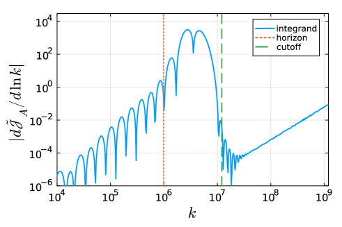
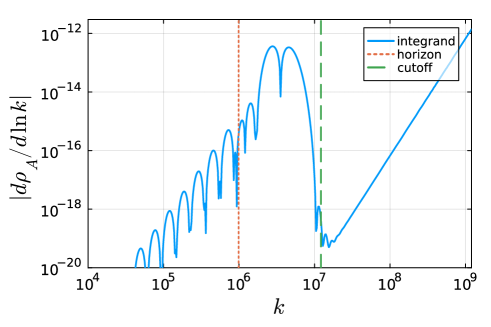
Figure 7: Absolute values of the integrand of $\tilde{\cal J}_{A}$, $d\tilde{\cal J}_{A}/d\ln k$ (left), and the integrand of $\delta\rho_{A}$, $d\delta\rho_{A}/d\ln k$ (right), as a function of $k$ in units of $aH$ at $y=0$. The input parameters are the same as in Figure 1, but $m_{Q}^{\rm in}=4.56$ and $y=13.8$ are taken. The comoving scale that exits the horizon (dotted, ‘horizon’) and the cutoff scale (dashed, ‘cutoff’) are also shown.

To verify that the $k$-integral is executed properly with the cutoff, $k_{\rm cut}$, given in Eq. (3.7), we present the integrands of $\tilde{\cal J}_{A}$ and $\delta\rho_{A}$. The integrands are defined in the logarithmic scale as

$$\tilde{\cal J}_{A} =\int d\ln k\frac{d\tilde{\cal J}_{A}}{d\ln k}\,,$$ (D.1)

$$\delta\rho_{A} =\int d\ln k\frac{d\delta\rho_{A}}{d\ln k}\,.$$ (D.2)

Figure 7 shows $|d\tilde{\cal J}_{A}/d\ln k|$ and $|d\delta\rho_{A}/d\ln k|$ for case (a) under initial condition (I). The parameters are the same as in Figure 1 and we choose $m_{Q}=4.56$. We show the results at $y=13.8$, which is just before the system reaches the perturbative limit. The cutoff scale, $k_{\rm cut}$, is shown by the vertical dashed lines. For reference, the comoving scale that exits the horizon at that time, $k=aH\,(=e^{y})$, is shown by the vertical dotted lines; the modes with $k$ smaller than this scale are outside the horizon.

We find that the modes between $aH$ and $k_{\rm cut}$ dominate the integral. The modes with $k>k_{\rm cut}$ correspond to the Bunch-Davies vacuum and should not be included in $\tilde{\cal J}_{A}$ or $\delta\rho_{A}$. The figure clearly shows that $k_{\rm cut}$ properly eliminates the Bunch-Davies vacuum contribution. Note that Ref. [Iarygina:2023mtj] adopts a subtraction scheme in which the Bunch-Davies vacuum contribution is subtracted from the integrand. Both approaches yield similar results.

Appendix E Slow-roll approximation

In this section, we verify the accuracy of the slow-roll approximation, i.e., $\tilde{\chi}^{\prime\prime}=m^{\prime\prime}_{Q}=\dot{H}=0$ and $\delta_{Q1}=-(\delta_{Q1}+\delta_{Q2})=\sqrt{\epsilon_{Q_{E}}}$.

Figure 8 shows the results for $m_{Q}^{\rm in}=4.47$ and $4.56$ in the left and right panels, respectively. The solid lines in the top four panels (‘Full result’) show the derivatives of the background fields, $m^{\prime}_{Q}$, $\xi\,(=\lambda\tilde{\chi}^{\prime}/2)$, $\delta_{Q1}$, and $-(\delta_{Q1}+\delta_{Q2})$, for case (a) under initial condition (I), which is associated with the dynamics shown in Figure 1. We have verified that $|\dot{H}|/H^{2}\lesssim\order{10^{-3}}$ is satisfied. The dashed lines (‘Slow-roll w BR’) and the dotted lines (‘Slow-roll w/o BR’) show $m^{\prime}_{Q}$ and $\xi$ given in Eqs. (3.8) and (3.9), in which the numerical solutions are used for the quantities on the right-hand sides with and without the backreaction (BR) terms, respectively. We find that the full results and the slow-roll results with BR agree well for $m_{Q}^{\rm in}=4.47$ (left panels), except for the earlier stage of the dynamics, where the $m_{Q}^{\prime\prime}$ and $\tilde{\chi}^{\prime\prime}$ terms give the oscillatory behavior. However, the slow-roll results without BR deviate from them. This means that the BR terms contribute to $m^{\prime}_{Q}$ and $\tilde{\chi}^{\prime}$ even before the strong BR regime; thus, the BR terms should always be included. We find similar results for $m_{Q}^{\rm in}=4.56$ (right panels). The slow-roll results with BR deviate from the full results near the perturbative limit.

The bottom two panels of Figure 8 show $\delta_{Q1}$ (solid) and $-(\delta_{Q1}+\delta_{Q2})$ (dashed). We find that $-(\delta_{Q1}+\delta_{Q2})\simeq\sqrt{\epsilon_{Q_{E}}}$ (dotted) is a good approximation, except for the earlier stage of the dynamics and near the perturbative limit. In summary, the slow-roll approximation, $m_{Q}^{\prime\prime}=\tilde{\chi}^{\prime\prime}=0$ and $\delta_{Q1}+\delta_{Q2}=-\sqrt{\epsilon_{Q_{E}}}$, cannot describe the oscillatory behavior and the dynamics near the perturbative limit. We find similar results under initial condition (II) (Figure 9).

Figures 10 and 11 show the results for case (b) under initial conditions (I) and (II), respectively. We have verified that $|\dot{H}|/H^{2}\lesssim\order{10^{-3}}$ is satisfied. We find that the slow-roll results for $m^{\prime}_{Q}$ deviate from the full result. For instance, the result with $m_{Q}^{\rm in}=5.58$ under initial condition (I) shows that the slow-roll approximation, i.e., neglecting $m^{\prime\prime}_{Q}$ and $\tilde{\chi}^{\prime\prime}$, is invalid. On the other hand, the slow-roll approximation is relatively accurate for $\xi$. This is because the right-hand side of the equation of motion for $\tilde{\chi}$ is suppressed with a large $\kappa$ and $3\tilde{\chi}^{\prime}-\beta(\chi)/\lambda\simeq 0$ tends to hold. Regarding $\delta_{Q1}$ and $\delta_{Q2}$, the slow-roll approximation, $-(\delta_{Q1}+\delta_{Q2})\simeq\sqrt{\epsilon_{Q_{E}}}$, does not hold in the early stage of the dynamics, i.e., the oscillatory behavior cannot be captured by the approximation. Otherwise, the approximation roughly holds, except near the perturbative limit.

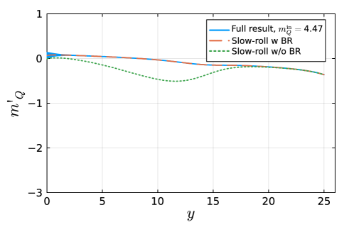
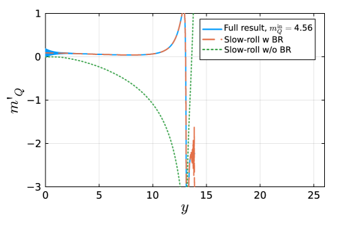
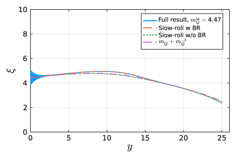
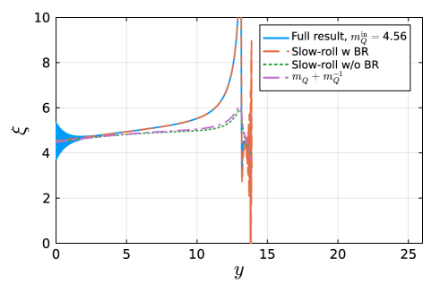
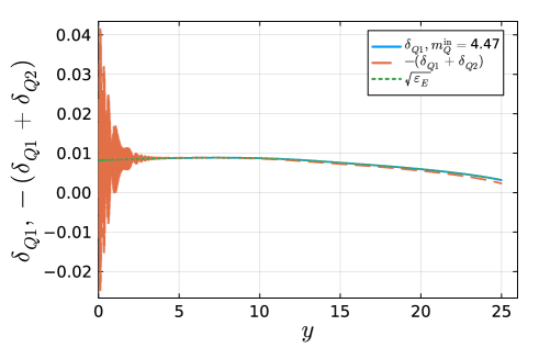
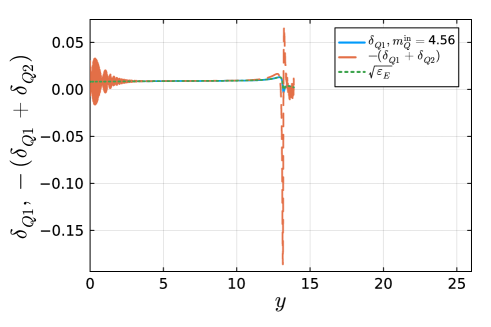
Figure 8: Time evolution of $m^{\prime}_{Q}$ (top), $\xi$ (middle), and $\delta_{Q1}$ and -($\delta_{Q1}+\delta_{Q2}$) (bottom), as a function of $y$. The parameters are the same as in Figure 1, i.e., case (a) under initial condition (I), but taking $m_{Q}^{\rm in}=4.47$ (left) and $4.56$ (right). ‘Full result’ shows the numerical solutions to the integro-differential equations. ‘Slow-roll w BR’ shows Eqs. (3.8) and (3.9) with $m_{Q}$, $\tilde{\chi}$, and the tensor modes on the right-hand sides from the numerical solutions. ‘Slow-roll w/o BR’ shows the results obtained by setting $\tilde{\cal J}_{A}=\tilde{\cal P}_{\chi}=0$. The dot-dashed lines in the middle panels show $\xi\simeq m_{Q}+m_{Q}^{-1}$, while the dotted lines in the bottom panels show $\delta_{Q1}+\delta_{Q2}\simeq-\sqrt{\epsilon_{Q_{E}}}$.

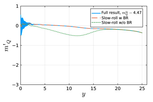
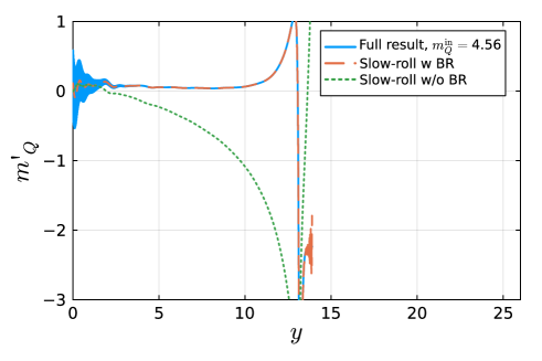
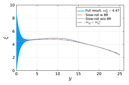
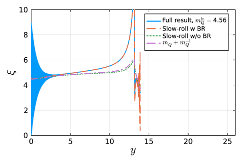
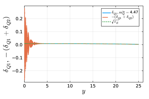
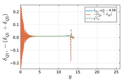
Figure 9: Same as Figure 8, but under initial condition (II), in which the initial conditions for the derivatives of the background fields are given by $m^{\prime}_{Q}=\tilde{\chi}^{\prime}=0$.

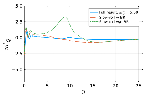
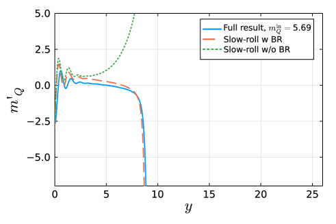
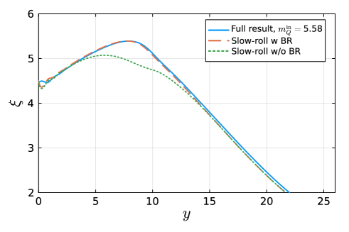
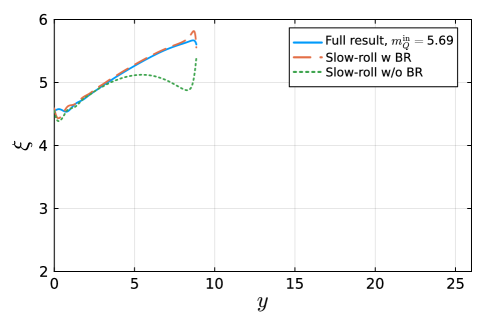
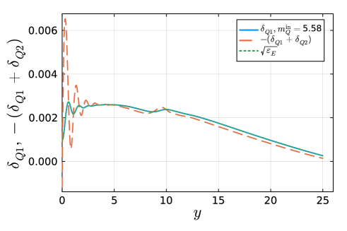
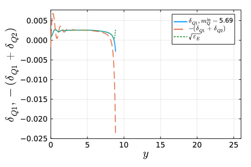
Figure 10: Same as Figure 8, but for case (b) under initial condition (I). The parameters are the same as in Figure 2, but taking $m_{Q}^{\rm in}=5.58$ (left) and $5.69$ (right).

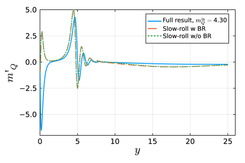
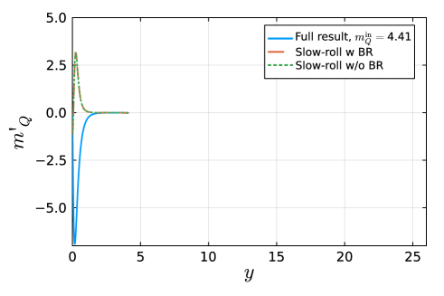
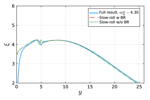
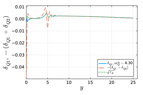
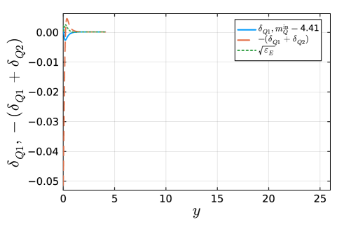
Figure 11: Same as Figure 10, but under initial condition (II). The parameters are the same as in Figure 3, but taking $m_{Q}^{\rm in}=4.30$ (left) and 4.41 (right).