A Lyapunov-Based Small-Gain Theorem for Fixed-Time Stability

Abstract

This paper introduces a novel Lyapunov-based small-gain methodology for establishing fixed-time stability (FxTS) guarantees in interconnected dynamical systems. Specifically, we consider interconnections in which each subsystem admits an individual fixed-time input-to-state stability (ISS) Lyapunov function that certifies FxT-ISS. We then show that if a nonlinear small-gain condition is satisfied, then the entire interconnected system is FxTS. Our results are analogous to existing Lyapunov-based small-gain theorems developed for asymptotic and finite-time stability, thereby filling an important gap in the stability analysis of interconnected dynamical systems. The proposed theoretical tools are further illustrated through analytical and numerical examples, including an application to fixed-time feedback optimization of dynamical systems without time-scale separation between the plant and the controller.

I Introduction

To address the growing demand for fast control and learning algorithms with greater accuracy and stronger robustness guarantees, significant research efforts have focused on developing tools that enable improved convergence properties. Finite-time stability (FTS) [bhatfinite] and control [zpjfinite] have attracted attention from the nonlinear controls community due to improved convergence and disturbance rejection properties. However, a drawback of finite-time stabilization is that the time by which the system is guaranteed to reach its equilibrium (i.e., the settling time) may grow unbounded with respect to the system’s initialization. This motivates the notion of fixed-time stability (FxTS), which distinguishes itself from FTS by further guaranteeing a uniform upper bound on the settling time. Following the introduction of Lyapunov conditions in [6104367] to verify FxTS for continuous-time autonomous systems, FxTS has received significant attention due to its ability to address challenges in a variety of engineering domains, such as control [9696292], network synchronization [hu2020fixed], optimization [10885949], learning [9760031], neural networks [CHEN2020412], etc. Despite the numerous advancements in the theory of FxTS, there are limited tools available that simplify the verification of FxTS for large scale systems. Current methods require the systems to satisfy restrictive structural requirements [9714166], certain interconnection conditions under a time-scale separation [10644358, 11239427], or trajectory-based small gain conditions [10886634].

The small-gain theorem is a fundamental tool for the stability analysis of interconnected systems. Originally developed for systems with linear gains [1098316], the small-gain theorem has been extended to those with nonlinear gains [jiang1994small] after the development of input-to-state stability (ISS) theory [sontag2008input]. In the past few decades, small-gain theory has been extended to hybrid systems [bao2018ios, liberzon2012small], stochastic systems [dragan1997small], discrete-time systems [jiang2004nonlinear, zhongping2008nonlinear], and infinite dimensional systems [mironchenko2021nonlinear, mironchenko2021small], to name a few. Moreover, to harness the power, applicability, and constructiveness of Lyapunov-based methods, considerable work has also been done to reformulate nonlinear small-gain theory in the sense of Lyapunov [jiang1996lyapunov, liberzon2014lyapunov, kawan2020lyapunov]. While the literature on nonlinear small-gain theory is indeed vast, extensions to systems with accelerated convergence are relatively recent and, for the most part, underdeveloped. Trajectory-based small-gain conditions were derived in [zpjfinite] for interconnected finite-time input-to-state stable systems, and a Lyapunov-based reformulation for networks was proposed in [sgfinite]. Following the development of the concept of fixed-time input-to-state stability (FxT ISS) [LOPEZRAMIREZ2020104775], a trajectory-based small-gain theorem was developed for interconnected FxT ISS systems in [10886634]. However, as acknowledged by the authors, the results are quite restrictive in that they contain additional conditions that depend on the settling-time function, its inverse, and several auxiliary functions that are used to upper bound the trajectories of the subsystems.

The main contribution of this paper is the introduction of a novel Lyapunov-based small-gain theorem to establish FxTS for interconnected FxT ISS subsystems. Specifically, we show that if each of the subsystems admit a FxT ISS Lyapunov function, and the gain functions —under a mild structural requirement— satisfy the nonlinear small-gain condition, then the overall interconnected system is FxTS. In this sense, our main result mirrors similar Lyapunov-based small gain theorems developed in the literature for the study of asymptotic stability and finite-time stability. However, as described in the paper, our results do not follow as simple extensions of previous results, but rather require the derivation of several new technical lemmas, which are presented in the Appendix for the sake of completeness.

After introducing the main analytical results, we present two numerical examples to illustrate our main results. In the first example we consider the interconnection of two systems with with homogeneous coupling terms. In the second example we consider the problem of fixed-time feedback optimization in dynamical systems [9075378, 8673636, bianchin2022online] without timescale separation, a problem that had not been addressed before.

The rest of this paper is organized as follows: Section II presents some mathematical preliminaries. Section III presents the main results. Section IV presents the application to feedback optimization, and Section V presents the conclusions.

II Preliminaries

II-A Notation

We use $\mathbb{R}_{\geq 0}$ to denote the set of nonnegative real numbers. A continuous function $\alpha:\mathbb{R}_{\geq 0}\to\mathbb{R}_{\geq 0}$ is said to be of class $\mathcal{K}$, denoted $\alpha\in\mathcal{K}$, if $\alpha(0)=0$ and $\alpha$ is strictly increasing. We use $\mathcal{K}_{\infty}$ to denote the set of $\alpha\in\mathcal{K}$ that satisfy $\lim_{s\to\infty}\alpha(s)=\infty$. Given $\alpha\in\mathcal{K}_{\infty}$, if there exists $n\in\mathbb{N}$ and constants $c_{i}>0$, $p_{i}>0$ for $i=1,...,n$ such that $\alpha(s)=\sum_{i=1}^{n}c_{i}s^{p_{i}}$ for $s\geq 0$, we say $\alpha$ is of class $\mathcal{K}_{\infty}^{+}$, denoted $\alpha\in\mathcal{K}_{\infty}^{+}$. Moreover, if $n=2$ with $p_{1}\in(0,1)$ and $p_{2}>1$, we say $\alpha\in\mathcal{K}_{\infty}^{\text{FxT}}$. Given $\alpha\in\mathcal{K}_{\infty}$, we use $\alpha^{-1}$ to denote its inverse. We define $\mathcal{K}_{\infty}^{-1}$ to be the class of functions $\alpha\in\mathcal{K}_{\infty}$ that satisfy $\alpha^{-1}\in\mathcal{K}_{\infty}^{+}$. A continuous function $\beta:\mathbb{R}_{\geq 0}\times\mathbb{R}_{\geq 0}\to\mathbb{R}_{\geq 0}$ is said to be of class $\mathcal{KL}^{\text{FXT}}$, denoted $\beta\in\mathcal{KL}^{\text{FXT}}$, if $\beta(\cdot,0)\in\mathcal{K}$ and for each fixed $r\geq 0$, $\beta(r,\cdot)$ is continuous, non-increasing and there exists a function $T:\mathbb{R}_{\geq 0}\to\mathbb{R}_{\geq 0}$ such that $\beta(r,t)=0$ for all $t\geq T(r)$. The mapping $T$ is called the settling time function. Given a measurable function $u:\mathbb{R}_{\geq 0}\to\mathbb{R}^{m}$ we denote $|u|_{\infty}=\text{ess}\sup_{t\geq 0}|u(t)|$, where $|\cdot|$ represents the Euclidean norm. We use $\mathcal{L}_{\infty}^{m}$ to denote the set of measurable functions $u:\mathbb{R}_{\geq 0}\to\mathbb{R}^{m}$ satisfying $|u|_{\infty}<\infty$. For a function $f:(a,b)\to\mathbb{R}$, the upper right Dini derivative at $t\in(a,b)$ is defined as $D^{+}f(t)=\limsup_{h\to 0^{+}}\frac{f(t+h)-f(t)}{h}$. Given a differentiable function $f:\mathbb{R}^{n}\to\mathbb{R}^{m}$, we use $\mathbf{J}_{f}(x)\in\mathbb{R}^{m\times n}$ to denote the Jacobian of $f$ evaluated at $x\in\mathbb{R}^{n}$. If $m=1$, we use $\nabla f(x)=\mathbf{J}_{f}(x)^{\top}$. If $\mathbf{J}_{f}(x)$ is continuous, we say $f$ is $\mathcal{C}^{1}$. We use $I_{n}\in\mathbb{R}^{n\times n}$ to denote the $n$-by-$n$ identity matrix. If $Q\in\mathbb{R}^{n\times n}$ is symmetric, we use $\overline{\lambda}(Q)$ and $\underline{\lambda}(Q)$ to denote its largest and smallest eigenvalue, respectively. If $Q\in\mathbb{R}^{n\times m}$, we use $\overline{\mu}(Q)$ to denote its largest singular value. We present a simple lemma that will be instrumental for our results

Lemma 1

Given $\underline{p}\leq p\leq\overline{p}$, the following holds

$$x^{p}\leq x^{\underline{p}}+x^{\overline{p}},$$

for all $x\geq 0$. $\square$

Proof:

For $x\in[0,1]$ we have $x^{p}\leq x^{\underline{p}}$, and for $x\geq 1$ we have $x^{p}\leq x^{\overline{p}}$. We combine both cases to establish the result. ∎

II-B Fixed-Time stability

Consider the following class of autonomous systems

$$\dot{x}=f(x),\quad x(0)=x_{0},$$ (1)

where $x\in\mathbb{R}^{n}$ is the state and $f:\mathbb{R}^{n}\to\mathbb{R}^{n}$ is a continuous vector field with $f(0)=0$. We will state some definitions that are inspired by the results of [6104367].

Definition 1

The origin of (1) is said to be uniformly globally fixed-time stable (FxTS) if there exists $\beta\in\mathcal{KL}^{\text{FXT}}$ such that for each $x_{0}\in\mathbb{R}^{n}$, every solution of (1) exists for $t\geq 0$ and satisfies $|x(t)|\leq\beta(|x_{0}|,t)$ for all $t\geq 0$, where the settling time function $T$ of $\beta$ is uniformly bounded with $T(0)=0$. $\square$

Definition 2

A continuous function $V:\mathbb{R}^{n}\to\mathbb{R}_{\geq 0}$ is said to be a FxTS Lyapunov function for (1) if

1. There exists $\underline{\alpha},\overline{\alpha}\in\mathcal{K}_{\infty}$ such that

   $$\underline{\alpha}(|x|)\leq V(x)\leq\overline{\alpha}(|x|),$$ (2)

   for all $x\in\mathbb{R}^{n}$.

2. There exists $\Psi\in\mathcal{K}_{\infty}^{\text{FxT}}$ such that the following holds

   $$D^{+}V(x(t))\leq-\Psi(V(x(t))),$$ (3)

   along the trajectories of the system (4) for all $t\geq 0$. $\square$

It was shown in [6104367] that the origin of (1) is FxTS if it admits a FxTS Lyapunov function. Moreover, if $\Psi$ in (3) is given by $\Psi(s)=as^{p}+bs^{q}$ with $a,b>0,p\in(0,1),q>1$, then the settling time of $\beta$ satisfies the following bound for all $x_{0}\in\mathbb{R}^{n}$:

$$T(x_{0})\leq\frac{1}{a(1-p)}+\frac{1}{b(q-1)}.$$

II-C Fixed-time input-to-state stability

Consider the following class of dynamical systems that also depend on an input:

$$\dot{x}=f(x,u),\quad x(0)=x_{0},$$ (4)

where $x\in\mathbb{R}^{n}$ is the state, $u\in\mathcal{L}_{\infty}^{m}$ is the input, and $f:\mathbb{R}^{n}\times\mathbb{R}^{m}\to\mathbb{R}^{n}$ is a continuous, non-Lipschitz vector field that satisfies $f(0,0)=0$. We will state some definitions and results from [LOPEZRAMIREZ2020104775] that will be particularly useful for our work

Definition 3

The system (4) is said to be fixed-time input-to-state stable (FxT ISS) if there exists $\beta\in\mathcal{KL}^{\text{FXT}}$ and $\varrho\in\mathcal{K}$ such that for each $x_{0}\in\mathbb{R}^{n}$ and $u\in\mathcal{L}_{\infty}^{m}$, every solution $x(t)$ of (4) exists for $t\geq 0$ and satisfies

$$|x(t)|\leq\beta(|x_{0}|,t)+\varrho(|u|_{\infty}),$$

for all $t\geq 0,$ where the settling time function $T$ of $\beta$ is continuous and uniformly bounded, with $T(0)=0$. $\square$

Definition 4

A $\mathcal{C}^{1}$ function $V:\mathbb{R}^{n}\to\mathbb{R}_{\geq 0}$ is said to be a FxT ISS Lyapunov function for (4) if it satisfies item 1 of Definition 2 and there exists $\chi\in\mathcal{K}_{\infty}$ and $\Psi\in\mathcal{K}_{\infty}^{\text{FxT}}$ such that the following holds

$$V(x)\geq\chi(|u|)\Rightarrow\nabla V(x)^{\top}f(x,u)\leq-\Psi(V(x)),$$ (5)

for all $x\in\mathbb{R}^{n}$ and $u\in\mathbb{R}^{m}$. $\square$

It is shown in [LOPEZRAMIREZ2020104775] that if (4) admits a FxT ISS Lyapunov function, it is FxT ISS. Moreover, it directly follows from definition that if (4) is FxT ISS, then the origin of system (4) with $u(t)\equiv 0$ is FxTS.

III Main Results

III-A Analysis

We consider interconnections of the following form

$$\dot{x}_{1} =f_{1}(x_{1},x_{2})$$ (6a)

$$\dot{x}_{2} =f_{2}(x_{1},x_{2}),$$ (6b)

where $x_{i}\in\mathbb{R}^{n_{i}}$ are the states and $f_{i}:\mathbb{R}^{n_{1}}\times\mathbb{R}^{n_{2}}\to\mathbb{R}^{n_{i}}$ are continuous vector fields with $f_{1}(0,0)=f_{2}(0,0)=0$, see Figure 1. Our primary goal is to derive lower order conditions on the subsystems (6a) and (6b) that allow us to establish FxTS of the system (6). To address this, we propose a Lyapunov-based small gain approach and make the following assumption on (6):

Assumption 1

Consider the system (6) and, for each $i=1,2$, with $j=3-i$, there exists $\mathcal{C}^{1}$ functions $V_{i}:\mathbb{R}^{n_{i}}\to\mathbb{R}_{+}$ satisfying the following conditions:

1. There exists $\underline{\alpha}_{i},\overline{\alpha}_{i}\in\mathcal{K}_{\infty}$ such that

   $$\underline{\alpha}_{i}(|x_{i}|)\leq V(x_{i})\leq\overline{\alpha}_{i}(|x_{i}|),$$ (7)

   for all $x_{i}\in\mathbb{R}^{n_{i}}$.

2. There exists $\gamma_{i}\in\mathcal{K}_{\infty}$ and $\Psi_{i}\in\mathcal{K}_{\infty}^{\text{FxT}}$ such that the following holds

   $$V_{i}(x_{i})\geq\gamma_{i}(V_{j}(x_{j}))$$

   $$\Rightarrow\nabla V_{i}(x_{i})^{\top}f_{i}(x_{1},x_{2})\leq-\Psi_{i}(V_{i}(x_{i})),$$ (8)

   for all $x\in\mathbb{R}^{n_{1}+n_{2}}$. $\square$

In other words, we simply require that each $x_{i}$ subsystem is FxT ISS with respect to “input” $x_{j}$, and that there exists a FxT ISS Lyapunov function to establish this property. Note that although (2) is not exactly in the form (5), it can be placed into the form (5) by leveraging (7). We are now ready to state the first main result of the paper:

Theorem 1

Let system (6) satisfy Assumption 1 and suppose, for each $i=1,2$, there exists $\hat{\gamma}_{i}\in\mathcal{K}_{\infty}^{+}\cup\mathcal{K}_{\infty}^{-1}$ such that the following conditions are satisfied:

1. $\hat{\gamma}_{i}(s)>\gamma_{i}(s)$ for all $s>0$.

2. $\hat{\gamma}_{1}\circ\hat{\gamma}_{2}(s)<s$ for all $s>0$.

Then, the origin of the system (6) is FxTS. $\square$

Figure 1: A block diagram depicting the interconnection (6).

Proof:

Let $\sigma_{\lambda}\in\mathcal{K}_{\infty}^{+}$ take the form $\sigma_{\lambda}(s)=s^{\lambda}$ for $\lambda\geq 1$, and consider the FxTS Lyapunov function candidate

$$V(x) =\max\{\sigma_{\lambda}\circ V_{1}(x_{1}),\sigma_{\lambda}\circ\hat{\gamma}_{1}\circ V_{2}(x_{2}),\sigma_{\lambda}\circ V_{2}(x_{2}),$$

$$~~~\sigma_{\lambda}\circ\hat{\gamma}_{2}\circ V_{1}(x_{1})\},$$ (9)

where $\lambda$ is a sufficiently large constant such that $\sigma_{\lambda}\circ\hat{\gamma}_{2}\circ V_{1}(x_{1})$ and $\sigma_{\lambda}\circ\hat{\gamma}_{1}\circ V_{2}(x_{2})$ are FxT ISS Lyapunov functions of the (6a) and (6b) subsystems, respectively. As shown in Lemmas 5 and 6, such a $\lambda\geq 1$ always exists. Moreover, since $\lambda\geq 1$, it follows from Lemma 5 that $\sigma_{\lambda}\circ V_{1}(x_{1})$ and $\sigma_{\lambda}\circ V_{2}(x_{2})$ are also FxT ISS Lyapunov functions of the (6a) and (6b) subsystems, respectively. Then, for $i,j\in\{1,2\}$, we define

$$\sigma_{i1}(s) :=\sigma_{\lambda}(s)$$ (10a)

$$\sigma_{i2}(s) :=\sigma_{\lambda}\circ\hat{\gamma}_{3-i}(s)$$ (10b)

$$V_{ij}(x_{i}) :=\sigma_{ij}\circ V_{i}(x_{i}).$$ (10c)

Let $x(0)\in\mathbb{R}^{n}$ and let $x(\cdot)$ be a maximal solution to system (6) from $x(0)$, defined for all $t\in[0,T_{\text{max}})$, with $T_{\text{max}}\in(0,\infty]$. Each $V_{ij}(x_{i})$ is a FxT ISS Lyapunov function for the $x_{i}$ subsystem and, hence, satisfies the following properties for each $i,j\in\{1,2\}$:

1. The inequalities

   $$\underline{\alpha}_{ij}(|x_{i}|)\leq V_{ij}(x_{i})\leq\overline{\alpha}_{ij}(|x_{i}|),$$

   hold for all $x_{i}\in\mathbb{R}^{n_{i}}$, where $\underline{\alpha}_{ij}=\sigma_{ij}\circ\underline{\alpha}_{i}$ and $\overline{\alpha}_{ij}=\sigma_{ij}\circ\overline{\alpha}_{i}$

2. There exists $\Psi_{ij}\in\mathcal{K}_{\infty}^{\text{FxT}}$ such that:

   $$V_{ij}(x_{i})\geq\gamma_{ij}\circ V_{3-i}(x_{3-i})$$

   $$\Rightarrow D^{+}V_{ij}(x_{i})\leq-\Psi_{ij}(V_{ij}(x_{i})),$$ (11)

   holds for all $0\leq t<T_{\text{max}}$ and $x\in\mathbb{R}^{n_{1}+n_{2}}$, where $\gamma_{ij}=\sigma_{ij}\circ\hat{\gamma}_{i}$.

Next, define

$$\underline{\alpha}(s) =\min_{i,j=1,2}\underline{\alpha}_{ij}\left(\frac{s}{\sqrt{2}}\right),\quad\overline{\alpha}(s)=\max_{i,j=1,2}\overline{\alpha}_{ij}(s).$$

It is easy to verify that $V(x)=\max_{i,j=1,2}V_{ij}(x_{i})$ satisfies (2) with $\underline{\alpha},\overline{\alpha}\in\mathcal{K}_{\infty}$. Now, consider some $t\in[0,T_{\text{max}})$ where $V(x)=\sigma_{ij}\circ V_{i}(x_{i})$, which leads to four cases:

1. If $i=1$ and $j=1$, we have that $\sigma_{11}\circ V_{1}(x_{1})\geq\sigma_{22}\circ V_{2}(x_{2})$. This implies $V_{1}(x_{1})\geq\hat{\gamma}_{1}\circ V_{2}(x_{2})$, and thus $V_{11}(x_{1})\geq\gamma_{11}\circ V_{2}(x_{2})$. By (2), we have $\nabla V_{11}(x_{1})^{\top}f_{1}(x_{1},x_{2})\leq-\Psi_{11}(V_{11}(x_{1}))$

2. If $i=1$ and $j=2$, we have $\sigma_{12}\circ V_{1}(x_{1})\geq\sigma_{21}\circ V_{2}(x_{2})$, which implies $\hat{\gamma}_{2}\circ V_{1}(x_{1})\geq V_{2}(x_{2})$. By the small gain condition, we also have $V_{1}(x_{1})\geq\hat{\gamma}_{1}\circ V_{2}(x_{2})$, which implies $V_{12}(x_{1})\geq\gamma_{12}\circ V_{2}(x_{2})$. Hence, by (2), it follows that $\nabla V_{12}(x_{1})^{\top}f_{1}(x_{1},x_{2})\leq-\Psi_{12}(V_{12}(x_{1}))$

3. If $i=2$ and $j=1$, we have $\sigma_{21}\circ V_{2}(x_{2})\geq\sigma_{12}\circ V_{1}(x_{1})$, which implies $V_{2}(x_{2})\geq\hat{\gamma}_{2}\circ V_{1}(x_{1})$, and thus $V_{21}(x_{2})\geq\gamma_{21}\circ V_{1}(x_{1})$. By (2), we have $\nabla V_{21}(x_{2})^{\top}f_{2}(x_{1},x_{2})\leq-\Psi_{21}(V_{21}(x_{2}))$.

4. If $i=2$ and $j=2$, we have $\sigma_{22}\circ V_{2}(x_{2})\geq\sigma_{11}\circ V_{1}(x_{1})$, which implies $\hat{\gamma}_{1}\circ V_{2}(x_{2})\geq V_{1}(x_{1})$. By the small gain condition, we have $V_{2}(x_{2})\geq\hat{\gamma}_{2}\circ V_{1}(x_{1})$, which implies $V_{22}(x_{2})\geq\gamma_{22}\circ V_{1}(x_{1})$. Hence, (2) yields $\nabla V_{22}(x_{2})^{\top}f_{2}(x_{1},x_{2})\leq-\Psi_{22}(V_{22}(x_{2}))$.

Since $\Psi_{i,j}\in\mathcal{K}_{\infty}^{\text{FxT}}$ for each $i,j$, it follows from Lemma 2 that there exists some $\Psi\in\mathcal{K}_{\infty}^{\text{FxT}}$ such that

$$\Psi(s)\leq\min_{i,j=1,2}\Psi_{ij}(s),\quad\forall s\geq 0.$$

Now we can define $I(t)=\{(i,j):V(x(t))=V_{ij}(x_{i}(t))\}$ for $t\in[0,T_{\text{max}})$, and we can take the upper right Dini derivative of $V$ along the trajectories of (6) to obtain

$$D^{+}V(x(t)) =\max_{(i,j)\in I(t)}D^{+}V_{ij}(x_{i}(t))$$

$$=\max_{(i,j)\in I(t)}\nabla V_{ij}(x_{i}(t))^{\top}f_{i}(x_{1}(t),x_{2}(t))$$

$$\leq\max_{(i,j)\in I(t)}-\Psi_{ij}(V_{ij}(x_{i}(t)))$$

$$\leq\max_{(i,j)\in I(t)}-\Psi(V_{ij}(x_{i}(t)))$$

$$=-\Psi(V(x(t))),$$

where the first equality follows from [giorgi1992dini, Lemma 2.9].The trajectories are bounded on $[0,T_{\text{max}})$, and hence they are defined for all $t\geq 0$. This concludes the proof. ∎

Our approach is inspired by the ideas from [jiang1996lyapunov, sgfinite], in that we leverage the gain functions $\gamma_{i}$ to construct, for the interconnected system, a FxTS Lyapunov function candidate defined in the max form (9). Since the constructed FxTS Lyapunov function is possibly non-smooth, we must rely on the Dini derivative formulation in (3) to establish FxTS. To ensure that the FxT ISS Lyapunov function properties are preserved, we also utilize the power-function-based scaling technique introduced in [sgfinite] (this is the role of $\sigma_{\lambda}$). However, one important distinction to note is that since [sgfinite] is only concerned with finite time stability notions, it is sufficient in their setting for the gains $\hat{\gamma}_{i}(\cdot)$ to only have a class $\mathcal{K}_{\infty}^{+}$ approximation near the origin. Since we are concerned with the global notion of fixed-time stability, we now require that the class $\mathcal{K}_{\infty}^{+}$ approximation holds globally. One challenge that arises is that if $\hat{\gamma}_{1},\hat{\gamma}_{2}\in\mathcal{K}_{\infty}^{+}$, the small-gain condition will never be satisfied if there is a $\hat{\gamma}_{i}$ containing terms with different powers. To address this, we also allow for the gains $\hat{\gamma}_{i}$ to be class $\mathcal{K}_{\infty}^{-1}$, and we show in the Lemma 6 of the Appendix that such functions can also be appropriately scaled to preserve the FxT ISS Lyapunov function property.

Remark 1

While most functions in $\mathcal{K}_{\infty}^{-1}$ do not have a closed-form expression, this is not particularly problematic for our work. Indeed, if $\hat{\gamma}_{i}\in\mathcal{K}_{\infty}^{-1}$, then $\hat{\gamma}_{i}^{-1}\in\mathcal{K}_{\infty}^{+}$, so we can use the following equivalence

$$V_{i}(x_{i})\geq\hat{\gamma}_{i}(V_{j}(x_{j}))\Longleftrightarrow\hat{\gamma}_{i}^{-1}(V_{i}(x_{i}))\geq V_{j}(x_{j}),$$

to verify (2) in a simplified manner. Moreover, if $\hat{\gamma}_{1}\in\mathcal{K}_{\infty}^{+}$ and $\hat{\gamma}_{2}\in\mathcal{K}_{\infty}^{-1}$, we can leverage the following fact

$$\hat{\gamma}_{1}\circ\hat{\gamma}_{2}(s)<s\Longleftrightarrow\hat{\gamma}_{1}(s)<\hat{\gamma}_{2}^{-1}(s),$$ (12)

to verify the small-gain condition. Since $\hat{\gamma}_{2}^{-1}\in\mathcal{K}_{\infty}^{+}$, the condition $\hat{\gamma}_{1}(s)<\hat{\gamma}_{2}^{-1}(s)$ can be checked using straightforward methods, such as by applying Lemma 1. This is further detailed in the following example. $\square$

III-B Second-Order example

Consider the dynamics

$$\dot{x} =f(x)+\varepsilon_{1}\left(\lfloor y\rceil^{p}+\lfloor y\rceil^{q}\right)$$ (13a)

$$\dot{y} =g(y)-\varepsilon_{2}\lfloor x\rceil^{r},$$ (13b)

where $p,q,r>0$ and $\lfloor\cdot\rceil^{a}=|\cdot|^{a}\text{sgn}(\cdot)$. We assume that $f(\cdot)$ and $g(\cdot)$ are continuous vector fields such that the origins of the systems $\dot{x}=f(x)$ and $\dot{y}=g(y)$ are FxTS. We also assume that they admit quadratic FxTS Lyapunov functions $V(x)=x^{2}$ and $W(y)=y^{2}$, respectively. We will show that the origin for the system (13) is FxTS, as long as $\varepsilon_{1},\varepsilon_{2}>0$ are sufficiently small and $p,q,r$ satisfy some conditions specified below.

Theorem 2

Consider the system (13) with $p,q,r>0$ and $f:\mathbb{R}\to\mathbb{R},g:\mathbb{R}\to\mathbb{R}$ are continuous vector fields for which there exists $m_{1},m_{2}>0,\alpha_{1},\alpha_{2}\in(0,1)$, and $\beta_{1},\beta_{2}>1$ such that the following hold

$$2xf(x) \leq-2m_{1}|x|^{2\alpha_{1}}-2m_{1}|x|^{2\beta_{1}}$$

$$2yg(y) \leq-2m_{2}|y|^{2\alpha_{2}}-2m_{2}|y|^{2\beta_{2}},$$

for all $x,y\in\mathbb{R}$. Moreover, let $L_{r}=\max(1,2^{r-1})$ and suppose $pr,qr\in[\alpha_{2},\beta_{2}]$ and $\varepsilon_{1},\varepsilon_{2}$ satisfy

$$0<\varepsilon_{1}^{r}\varepsilon_{2}<\frac{m_{1}^{r}m_{2}}{2^{r}L_{r}^{\frac{1}{2}}}.$$ (15)

Then, the origin of (13) is FxTS. $\square$

Proof:

Taking $V(x)=x^{2}$ and $W(y)=y^{2}$, we have:

$$\dot{V} =2xf(x)+2\varepsilon_{1}x\lfloor y\rceil^{p}+2\varepsilon_{1}x\lfloor y\rceil^{q}$$

$$\leq-2m_{1}V^{\alpha_{1}}-2m_{1}V^{\beta_{1}}+2|x|(\varepsilon_{1}|y|^{p}+\varepsilon_{1}|y|^{q}).$$

Let $c_{1}\in(0,m_{1})$, which yields the following implication

$$|x|>\frac{\varepsilon_{1}}{m_{1}-\frac{1}{2}c_{1}}(|y|^{p}+|y|^{q})\Rightarrow\dot{V}\leq-c_{1}V^{\alpha_{1}}-c_{1}V^{\beta_{1}}.$$

Thus, we have

$$\gamma_{1}(s) =\left(\frac{\varepsilon_{1}}{m_{1}-\frac{1}{2}c_{1}}\right)^{2}(s^{\frac{p}{2}}+s^{\frac{q}{2}})^{2}$$

$$\leq 2\left(\frac{\varepsilon_{1}}{m_{1}-\frac{1}{2}c_{1}}\right)^{2}(s^{p}+s^{q}).$$

For the $y$ subsystem, we have

$$\dot{W} =2yg(y)-2\varepsilon_{2}y\lfloor x\rceil^{r}$$

$$\leq-m_{2}W^{\alpha_{2}}-m_{2}W^{\beta_{2}}+\frac{\varepsilon_{2}^{2}}{m_{2}}|x|^{2r}.$$

If we fix some $c_{2}\in(0,m_{2})$, we obtain the following

$$\dot{W} \leq-c_{2}W^{\alpha_{2}}-c_{2}W^{\beta_{2}}$$

$$~~~+\left(\frac{\varepsilon_{2}^{2}}{m_{2}}|x|^{2r}-(m_{2}-c_{2})\left(W^{\alpha_{2}}+W^{\beta_{2}}\right)\right).$$

Let $L_{r}=\max(1,2^{r-1})$, and suppose $p,q,r$ satisfy $pr,qr\in[{\alpha_{2}},{\beta_{2}}]$. We want $\varepsilon_{1},\varepsilon_{2}$ sufficiently small such that

$$\gamma_{2}^{-1}(s):=\left(\frac{m_{2}(m_{2}-c_{2})}{L_{r}\varepsilon_{2}^{2}}\right)^{\frac{1}{r}}\left(s^{\frac{\alpha_{2}}{r}}+s^{\frac{\beta_{2}}{r}}\right)>\gamma_{1}(s),$$ (16)

for all $s>0$. By Lemma 1, it suffices to have

$$\left(\frac{m_{2}(m_{2}-c_{2})}{L_{r}\varepsilon_{2}^{2}}\right)^{\frac{1}{r}}\geq\frac{4\varepsilon_{1}^{2}}{(m_{1}-\frac{1}{2}c_{1})^{2}},$$

which can be obtained whenever

$$\varepsilon_{1}^{r}\varepsilon_{2}\leq\frac{(m_{1}-\frac{1}{2}c_{1})^{r}m_{2}^{\frac{1}{2}}(m_{2}-c_{2})^{\frac{1}{2}}}{2^{r}L_{r}^{\frac{1}{2}}}.$$ (17)

Now, suppose $V(x)<\gamma_{2}^{-1}(W(y))$, which means:

$$|x|^{2}<\left(\frac{m_{2}(m_{2}-c_{2})}{L_{r}\varepsilon_{2}^{2}}\right)^{\frac{1}{r}}\left(W^{\frac{\alpha_{2}}{r}}+W^{\frac{\beta_{2}}{r}}\right).$$

Raising to the $r$ power yields:

$$|x|^{2r} \leq\frac{m_{2}(m_{2}-c_{2})}{\varepsilon_{2}^{2}}(W^{\alpha_{2}}+W^{\beta_{2}}).$$

Thus,

$$\dot{W}\leq-c_{2}W^{\alpha_{2}}-c_{2}W^{\beta_{2}},\quad W(y)>\gamma_{2}(V(x)).$$

Recall that $c_{1}$ and $c_{2}$ are arbitrary. Hence, if $\varepsilon_{1}^{r}\varepsilon_{2}$ satisfies (15), it follows immediately that $c_{1},c_{2}$ can be chosen such that $\varepsilon_{1}^{r}\varepsilon_{2}$ also satisfies (17). Then (16) implies $\gamma_{2}(s)<\gamma_{1}^{-1}(s)$ for all $s>0$. We can pick $\varepsilon>0$ such that (12) is satisfied with $\hat{\gamma}_{i}(s)=(1+\varepsilon)\gamma_{i}(s)$, allowing us to conclude that the small-gain condition is satisfied. Hence, the origin of the system (13) is FxTS. ∎

To verify our results numerically, we plot the trajectories of (13) with varying initial conditions, where the parameters are chosen to yield the following system

$$\dot{x} =-x^{\frac{1}{3}}-x^{3}+0.3\left(\lfloor y\rceil^{2}+\lfloor y\rceil^{2.5}\right)$$ (18a)

$$\dot{y} =-\lfloor y\rceil^{\frac{1}{2}}-\lfloor y\rceil^{2}-0.1\lfloor x\rceil^{\frac{4}{9}}.$$ (18b)

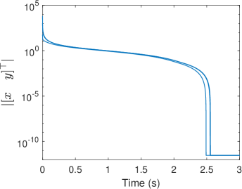
Figure 2: Trajectories of system (18) with varying $x(0),y(0)$.

It can be verified that these choice of parameters satisfy (15). The trajectories are shown in Figure 2, illustrating the FxTS property.

Remark 2

One important observation that can be made is that the presence of multiple exponents of $V$ in the classical FxTS and FxT ISS Lyapunov bounds in (3) and (5) allows us to handle $\mathcal{K}_{\infty}^{+}$ gains and interconnections that contain terms with differing exponents. For standard Lyapunov-based nonlinear small-gain theory [jiang1996lyapunov], the structure of the rate of decrease of the Lyapunov function (upon satisfaction of the ISS condition) results in a limited class of admissible gain functions. Even in the case of finite-time ISS [sgfinite] for interconnections, gain functions in $\mathcal{K}_{\infty}^{+}$ often only contain one term, the the exponents of the different gain functions need to multiply to 1. Indeed, if the origins of $\dot{x}=f(x)$ and $\dot{x}=g(x)$ are only assumed to be finite-time stable, then (13) will not satisfy the finite-time small-gain condition from [sgfinite] if $pr\neq 1$ or $qr\neq 1$. In our setting, this can be relaxed by leveraging the different exponents of $V$ and Lemma 1. Instead of precisely requiring $pr=qr=1$, or equivalently $p=q=\frac{1}{r}$, we now only require $pr,qr\in[\alpha_{2},\beta_{2}]$, which is a neighborhood of 1. This opens the door to generalizations of (13) that contain arbitrarily many cross terms between the subsystems, which will be of interest for future work. $\square$

IV Fixed-Time Feedback Optimization without Timescale Separation

In this section, we apply our results to study a practical problem of interest: feedback optimization of dynamical systems with fixed-time convergence. Standard feedback optimization schemes require inducing a timescale separation between the plant and controller [9075378, 8673636, bianchin2022online], as it enables stability analysis with tools from singular perturbation theory. This was also the case recently in [11239427], where the authors study multi-timescale fixed-time feedback optimization via composite Lyapunov functions. In contrast to this setting, we will show that, under certain conditions, approaching this problem with small-gain theory eliminates the need for a time-scale separation between the plant and controller. We consider plants of the form

$$\dot{x}=f(x,u),$$ (19)

where $x\in\mathbb{R}^{n}$ is the plant state and $u\in\mathbb{R}^{m}$ is a measurable and bounded control input. We will make the following assumption on the plant (19):

Assumption 2

For system (19), there exists $P\in\mathbb{R}^{n\times m}$ such that $f(Pu,u)=0$ for all $u\in\mathbb{R}^{m}$. Moreover, there exists $\ell,a,b>0,p\in(0,1),q>1$ such that

$$|x-Pu^{*}|^{2}\geq\ell^{2}|u-u^{*}|^{2}$$

$$\Rightarrow 2(x-Pu^{*})^{\top}f(x,u)\leq-a|x-Pu^{*}|^{2p}-b|x-Pu^{*}|^{2q},$$ (20)

for all $x\in\mathbb{R}^{n}$, $u\in\mathbb{R}^{m}$, and $u^{*}\in\mathbb{R}^{m}$. $\square$

Remark 3

The mapping $Pu$ is referred to as the steady-state mapping for the dynamics (19). In works that study feedback optimization using singular perturbation theory, it is typically the case that the steady state mapping is assumed to exhibit appropriate stability properties uniformly in $u$ (see, e.g [11239427, 9075378]). Here, we impose a very similar condition but in the FxT ISS framework. Essentially, we are requiring that for each fixed reference input $u^{*}$, the deviation $x-Pu^{*}$ is FxT ISS with respect to the deviation on the “input” $u-u^{*}$, which is established via the quadratic FxT ISS Lyapunov function $|x-Pu^{*}|^{2}$. We require that this property holds uniformly in $x,u$, and $u^{*}$. One class of systems satisfying Assumption 2 are those of the following form

$$\dot{x}=-\frac{A_{1}(x-Pu)}{|x-Pu|^{\tilde{p}}}-\frac{A_{2}(x-Pu)}{|x-Pu|^{\tilde{q}}},$$ (21)

where $A_{1},A_{2}\in\mathbb{R}^{n\times n}$ with $A_{1},A_{2}\succ 0$, $\tilde{p}\in(0,1)$, and $\tilde{q}<0$. The system (21) is a significant generalization of the plants considered in [10644358], where the authors used $m=n$ and $A_{1}=A_{2}=P=I_{n}$. $\square$

Our primary goal is to design a dynamic feedback law on $u$ to stabilize (19) while also optimizing a cost function $\phi(x,u)$. For this work, we will be primarily concerned with quadratic cost functions of the following form

$$\phi(x,u)=\frac{1}{2}x^{\top}Q_{1}x+b_{1}^{\top}x+\frac{1}{2}u^{\top}Q_{2}u+b_{2}^{\top}u,$$ (22)

where $Q_{1}\in\mathbb{R}^{n\times n},Q_{2}\in\mathbb{R}^{m\times m},b_{1}\in\mathbb{R}^{n}$, and $b_{2}\in\mathbb{R}^{m}$ with $Q_{1},Q_{2}\succ 0$. Since we wish to optimize (22) while stabilizing (19), we can substitute the steady state mapping $x=Pu$ into (22) to arrive at the following optimization problem

$$\min_{u}\Phi(u),$$ (23a)

where $\Phi(u)=\phi(Pu,u)$, with $\Phi(u)$ given by

$$\Phi(u):=\frac{1}{2}u^{\top}(P^{\top}Q_{1}P+Q_{2})u+(P^{\top}b_{1}+b_{2})^{\top}u.$$

To solve (23a), we propose a fixed-time gradient flow on $u$, i.e $\dot{u}=-\frac{\nabla\Phi(u)}{|\nabla\Phi(u)|^{\xi_{1}}}-\frac{\nabla\Phi(u)}{|\nabla\Phi(u)|^{\xi_{2}}}$, where $\xi_{1}\in(0,1)$ and $\xi_{2}<0$. Following the ideas from [11239427, 9075378], after evaluating $\nabla\Phi(u)$, we can substitute $x$ back into its steady state value to obtain the following feedback controller on $u$:

$$\dot{u}=-\frac{\mathcal{F}(x,u)}{|\mathcal{F}(x,u)|^{\xi_{1}}}-\frac{\mathcal{F}(x,u)}{|\mathcal{F}(x,u)|^{\xi_{2}}},$$ (24)

where $\mathcal{F}(x,u)$ is given by

$$\mathcal{F}(x,u)=P^{\top}Q_{1}x+Q_{2}u+P^{\top}b_{1}+b_{2}.$$

We are now ready to state the third main result of this paper:

Theorem 3

Consider system (19) interconnected with (24), where $\xi_{1}\in(0,1),\xi_{2}<0$, and system (19) satisfies Assumption 2. Moreover, suppose the following condition holds

$$\ell\frac{\overline{\mu}(P)\overline{\lambda}(Q_{1})}{\underline{\lambda}(Q_{2})}<1.$$ (25)

Then the point $(Pu^{*},u^{*})$ is rendered FxTS, where $u^{*}$ is the solution of (23a) and given by

$$u^{*}=-(P^{\top}Q_{1}P+Q_{2})^{-1}(P^{\top}b_{1}+b_{2}).$$

$\square$

Proof:

Denote $V(\tilde{x})=|\tilde{x}|^{2}$. We use the change of variables $\tilde{x}=x-Pu^{*}$ and $\tilde{u}=u-u^{*}$ to arrive at the following system

$$\dot{\tilde{x}} =f(\tilde{x}+Pu^{*},\tilde{u}+u^{*})$$ (26a)

$$\dot{\tilde{u}} =-\frac{\tilde{\mathcal{F}}(\tilde{x},\tilde{u})}{|\tilde{\mathcal{F}}(\tilde{x},\tilde{u})|^{\xi_{1}}}-\frac{\tilde{\mathcal{F}}(\tilde{x},\tilde{u})}{|\tilde{\mathcal{F}}(\tilde{x},\tilde{u})|^{\xi_{2}}},$$ (26b)

where $\tilde{\mathcal{F}}$ is given by

$$\tilde{\mathcal{F}}(\tilde{x},\tilde{u})=P^{\top}Q_{1}\tilde{x}+Q_{2}\tilde{u}.$$

By (25), we can pick $\varepsilon\in(0,\underline{\lambda}(Q_{2}))$ such that

$$\ell\frac{\overline{\mu}(P)\overline{\lambda}(Q_{1})}{\underline{\lambda}(Q_{2})-\varepsilon}<1.$$ (27)

Consider the FxT ISS Lyapunov function $W(\tilde{u})=|\tilde{u}|^{2}$ for (26b). It follows by direct computation that if $|\tilde{u}|\geq\frac{\overline{\mu}(P)\overline{\lambda}(Q_{1})}{\underline{\lambda}(Q_{2})-\varepsilon}|\tilde{x}|$, then the following inequalities hold:

$$\tilde{u}^{\top}P^{\top}Q_{1}\tilde{x}+\tilde{u}^{\top}Q_{2}\tilde{u} \geq\varepsilon|\tilde{u}|^{2}$$ (28a)

$$|P^{\top}Q_{1}\tilde{x}+Q_{2}\tilde{u}|^{\xi_{1}} \leq(2\overline{\lambda}(Q_{2}))^{\xi_{1}}|\tilde{u}|^{\xi_{1}}$$ (28b)

$$|P^{\top}Q_{1}\tilde{x}+Q_{2}\tilde{u}|^{-\xi_{2}} \geq\varepsilon^{-\xi_{2}}|\tilde{u}|^{-\xi_{2}}.$$ (28c)

We can then leverage the inequalities (28) with the FxT ISS Lyapunov function $W(\tilde{u})=|\tilde{u}|^{2}$ to obtain that, for $W(\tilde{u})\geq\left(\frac{\overline{\mu}(P)\overline{\lambda}(Q_{1})}{\underline{\lambda}(Q_{2})-\varepsilon}\right)^{2}V(\tilde{x})$, the following holds along the trajectories of (26b):

$$\dot{W} \leq-\frac{2\varepsilon}{(2\overline{\lambda}(Q_{2}))^{\xi_{1}}}|\tilde{u}|^{2(1-\frac{1}{2}\xi_{1})}-2\varepsilon^{1-\xi_{2}}|\tilde{u}|^{2(1-\frac{1}{2}\xi_{2})}$$

$$=-\frac{2\varepsilon}{(2\overline{\lambda}(Q_{2}))^{\xi_{1}}}W^{1-\frac{1}{2}\xi_{1}}-2\varepsilon^{1-\xi_{2}}W^{1-\frac{1}{2}\xi_{2}}.$$

Moreover, by Assumption 2, we know that for $V(\tilde{x})\geq\ell^{2}W(\tilde{u})$, the following holds along the trajectories of (26a)

$$\dot{V} =2\tilde{x}^{\top}f(\tilde{x}+Pu^{*},\tilde{u}+u^{*})\leq-aV^{p}-bV^{q}.$$

By (27) and Theorem 1, we conclude that the origin for the $(\tilde{x},\tilde{u})$ system is FxTS, which establishes the result. ∎

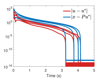
Figure 3: Trajectories of system (21) with (24) and varying initial conditions, where the parameters are given by (29) and (30).

To illustrate Theorem 2 numerically, we consider system (21) interconnected with the dynamic controller (24), where $x,u\in\mathbb{R}^{2}$ and

$$A_{1}=\begin{bmatrix}\frac{3}{2}&\frac{1}{5}\\ \frac{1}{5}&\frac{6}{5}\end{bmatrix},\quad A_{2}=\begin{bmatrix}\frac{6}{5}&\frac{3}{10}\\ \frac{3}{10}&\frac{8}{5}\end{bmatrix},\quad P=\begin{bmatrix}1&\frac{2}{3}\\ \frac{4}{3}&\frac{1}{3}\end{bmatrix},$$ (29)

and the cost function parameters of (22) are given by

$$Q_{1}=\begin{bmatrix}\frac{1}{2}&\frac{1}{4}\\ \frac{1}{4}&\frac{1}{5}\end{bmatrix},\quad Q_{2}=\begin{bmatrix}4&\frac{2}{5}\\ \frac{2}{5}&4\end{bmatrix},\quad b_{1}=\begin{bmatrix}3\\ 2\end{bmatrix},\quad b_{2}=\begin{bmatrix}1\\ 1\end{bmatrix}.$$ (30)

It is straightforward to verify that (21) with (29) satisfies Assumption 2 with $\ell=3.05$, and that the given parameters also satisfy (25). The trajectories are simulated with varying initial conditions in Figure 3.

V Conclusion

We introduced Lyapunov-based small-gain conditions for establishing fixed-time stability (FxTS) in interconnected dynamical systems. To the best of our knowledge, this is the first result of its kind in the literature on fixed-time stability. The theoretical developments are demonstrated through two illustrative examples. The first example, a second-order interconnection, provides a clear paradigm for applying the proposed tools to study interconnections of FxTS vector fields with homogeneous coupling terms. In the second example, we apply our results to analyze fixed-time feedback optimization in dynamical systems without requiring time-scale separation between the plant and the controller. Future work includes extending the result to large-scale networked and hybrid systems.

VI Appendix

Lemma 2

If $\alpha_{1},...,\alpha_{N}\in\mathcal{K}_{\infty}^{\text{FxT}}$, there exists $\alpha\in\mathcal{K}_{\infty}^{\text{FxT}}$ such that $\min_{k}\alpha_{k}(s)\geq\alpha(s)$ for all $s\geq 0$. $\square$

Proof:

Let $\alpha_{i}(s)=a_{i}s^{p_{i}}+b_{i}s^{q_{i}}$, where $p_{i}\in(0,1)$ and $q_{i}>1$ for $i=1,...,N$. Denote $m_{i}=\min(a_{i},b_{i})$ and $m=\min_{k}m_{k}$. By Lemma 1, we have that $\alpha_{i}(s)\geq ms^{r}$ for all $s\geq 0$, $i\in[N]$, and $r\in\cap_{j=1}^{N}[p_{j},q_{j}]=[\max_{k}p_{k},\min_{k}q_{k}]$. Fix $p\in[\max_{k}p_{k},1)$ and $q\in(1,\min_{k}q_{k}]$, then

$$\min_{k}\alpha_{k}(s)\geq\frac{m}{2}(s^{p}+s^{q})\in\mathcal{K}_{\infty}^{\text{FxT}},$$

which establishes the result. ∎

Lemma 3

Let $\Psi\in\mathcal{K}_{\infty}^{\text{FxT}}$ and $\sigma(s)=\sum_{i=1}^{n}c_{i}s^{r_{i}}$, where $1\leq r_{1}<r_{2}<..<r_{n}$ and $c_{i}>0$ for $i\in[n]$. Then, there exists $\tilde{\Psi}\in\mathcal{K}_{\infty}^{\text{FxT}}$ such that $\tilde{\Psi}(\sigma(s))\leq\Psi(s)\sigma^{\prime}(s)$ for all $s>0$. $\square$

Proof:

Let $\Psi(s)=as^{p}+bs^{q}$, where $p\in(0,1)$ and $q>1$. It then follows that $\sigma^{\prime}(s)=\sum_{i=1}^{n}r_{i}c_{i}s^{r_{i}-1}$, which yields

$$\Psi(s)\sigma^{\prime}(s) =\sum_{i=1}^{n}ar_{i}c_{i}s^{p+r_{i}-1}+\sum_{j=1}^{n}br_{j}c_{j}s^{q+r_{j}-1}$$

$$\geq ms^{p+r_{1}-1}+ms^{q+r_{n}-1},$$

where $m=\min(qr_{1}c_{1},br_{n}c_{n})$. We then postulate $\tilde{\Psi}\in\mathcal{K}_{\infty}^{\text{FxT}}$ of the form $\tilde{\Psi}(s)=\tilde{m}s^{\tilde{p}}+\tilde{m}s^{\tilde{q}}$, where $\tilde{p}=\frac{p+r_{1}-1}{r_{1}}\in(0,1)$ and $\tilde{q}=\frac{q+r_{n}-1}{r_{n}}>1$. Indeed, computations yield:

$$\tilde{\Psi}(\sigma(s)) \leq\tilde{m}\left(\sum_{i=1}^{n}c_{i}^{\tilde{p}}+n^{\tilde{q}-1}\sum_{j=1}^{n}c_{j}^{\tilde{q}}\right)(s^{p+r_{1}-1}+s^{q+r_{n}-1}),$$

where the inequality follows from Lemma 1 and the fact that $r_{i}\tilde{p},r_{i}\tilde{q}\in[p+r_{1}-1,q+r_{n}-1]$ for all $i\in[n]$. We can then pick $\tilde{m}$ sufficiently small to obtain the result. ∎

Lemma 4

Suppose $\gamma\in\mathcal{K}_{\infty}^{-1}$, and let $\Psi\in\mathcal{K}_{\infty}^{\text{FxT}}$. Then there exists $\lambda\geq 1$ and $\tilde{\Psi}\in\mathcal{K}_{\infty}^{\text{FxT}}$ such that $\varrho(s)\geq\tilde{\Psi}(\gamma^{\lambda}(s))$ for all $s>0$, where $\varrho(s)=\lambda\gamma^{\lambda-1}(s)\gamma^{\prime}(s)\Psi(s)$. $\square$

Proof:

Denote $\Psi(s)=as^{p}+bs^{q}$, where $p\in(0,1)$ and $q>1$ and let $\gamma^{-1}(s)=\sum_{i=1}^{n}c_{i}s^{r_{i}}$, where $0<r_{1}<r_{2}<...<r_{n}$ and $c_{i}>0$ for all $i\in[n]$. Note that $\gamma^{-1}(s)\geq c_{i}s^{r_{i}}$, which implies $\gamma(s)\leq\tilde{c}_{i}s^{\frac{1}{r_{i}}}$ for all $i\in[n]$ and $s\geq 0$, where $\tilde{c}_{i}=c_{i}^{-\frac{1}{r_{i}}}$. From this, we obtain the following:

$$\Psi(s) \geq\frac{a}{\tilde{c}_{i}^{pr_{i}}}\gamma^{pr_{i}}(s)+\frac{b}{\tilde{c}_{i}^{qr_{i}}}\gamma^{qr_{i}}(s)$$

$$=ac_{i}^{p}\gamma^{pr_{i}}(s)+bc_{i}^{q}\gamma^{qr_{i}}(s).$$

We define the constant $R:=\sum_{i=1}^{n}r_{i}c_{i}$, and we first consider the case of $\gamma(s)\in(0,1)$, which implies $\sum_{i=1}^{n}r_{i}c_{i}\gamma^{r_{i}-1}(s)\leq R\gamma^{r_{1}-1}(s)$. From the inverse function theorem, we obtain:

$$\varrho(s) =\frac{\lambda\gamma^{\lambda-1}(s)\Psi(s)}{\sum_{i=1}^{n}r_{i}c_{i}\gamma^{r_{i}-1}(s)}$$

$$\geq\frac{\lambda ac_{i}^{p}\gamma^{\lambda-1+pr_{i}}(s)+\lambda bc_{i}^{q}\gamma^{\lambda-1+qr_{i}}(s)}{R\gamma^{r_{1}-1}(s)}$$

$$\geq\tilde{m}_{i}\gamma^{\lambda+pr_{i}-r_{1}}(s)+\tilde{m}_{i}\gamma^{\lambda+qr_{i}-r_{1}}(s),$$

where $\tilde{m}_{i}=\frac{\lambda}{R}\min\left(ac_{i}^{p},bc_{i}^{q}\right)$. Choosing $i=1$ yields $\varrho(s)\geq\tilde{\Psi}_{1}(\gamma^{\lambda}(s))$, where $\tilde{\Psi}_{i}$ is given by

$$\tilde{\Psi}_{i}(s)=\tilde{m}_{i}s^{1-\frac{(1-p)r_{i}}{\lambda}}+\tilde{m}_{i}s^{1+\frac{(q-1)r_{i}}{\lambda}}.$$

Picking $\lambda>(1-p)r_{1}$ guarantees $\tilde{\Psi}_{1}\in\mathcal{K}_{\infty}^{\text{FxT}}$. Now, we consider the case of $\gamma(s)\geq 1$, which implies $\sum_{i=1}^{n}r_{i}c_{i}\gamma^{r_{i}-1}(s)\leq R\gamma^{r_{n}-1}(s)$. We can then perform similar calculations done above to obtain:

$$\varrho(s)\geq\tilde{m}_{i}\gamma^{\lambda+pr_{i}-r_{n}}(s)+\tilde{m}_{i}\gamma^{\lambda+qr_{i}-r_{n}}(s),\quad i\in[n].$$

If we choose $i=n$, we obtain $\varrho(s)\geq\tilde{\Psi}_{n}(\gamma^{\lambda}(s))$, where $\tilde{\Psi}_{n}\in\mathcal{K}_{\infty}^{\text{FxT}}$ if $\lambda>(1-p)r_{n}$. Since we assume $r_{1}<r_{n}$, it suffices to have $\lambda>(1-p)r_{n}$. By Lemma 2, we know that there exists $\tilde{\Psi}\in\mathcal{K}_{\infty}^{\text{FxT}}$ such that $\min(\tilde{\Psi}_{1}(s),\tilde{\Psi}_{n}(s))\geq\tilde{\Psi}(s)$ for all $s>0$. Putting both cases together, we obtain

$$\varrho(s)\geq\min\left(\tilde{\Psi}_{1}(\gamma^{\lambda}(s)),\tilde{\Psi}_{n}(\gamma^{\lambda}(s))\right)\geq\tilde{\Psi}(\gamma^{\lambda}(s)),$$

which establishes the result. ∎

Lemma 5

Suppose $V:\mathbb{R}^{n}\to\mathbb{R}_{+}$ is a FxT ISS Lyapunov function for (4). Then, if $\sigma(s)=\sum_{i=1}^{n}c_{i}s^{r_{i}}$, where $1\leq r_{1}<r_{2}<..<r_{n}$ and $c_{i}>0$ for $i\in[n]$, it follows that $\tilde{V}(x)=\sigma(V(x))$ is a FxT ISS Lyapunov function of (4). $\square$

Proof:

First, it is easy to verify that $\sigma(\underline{\alpha}(|x|))\leq\tilde{V}(x)\leq\sigma(\overline{\alpha}(|x|)).$ Let $\tilde{\chi}=\sigma\circ\chi$ and suppose $\tilde{V}(x)\geq\tilde{\chi}(|u|)$, which implies $\nabla V(x)^{\top}f(x,u)\leq-\Psi(V(x))$. Then we obtain:

$$\nabla\tilde{V}(x)^{\top}f(x,u) =\sigma^{\prime}(V(x))\nabla V(x)^{\top}f(x,u)$$

$$\leq-\Psi(V(x))\sigma^{\prime}(V(x)),$$

where $\Psi\in\mathcal{K}_{\infty}^{\text{FxT}}$ and $\sigma^{\prime}$ denotes the derivative of $\sigma$. By Lemma 3, we can find some $\tilde{\Psi}\in\mathcal{K}_{\infty}^{\text{FxT}}$ such that $\tilde{\Psi}(\sigma(s))\leq\Psi(s)\sigma^{\prime}(s)$ for all $s>0$. Then we obtain

$$\nabla\tilde{V}(x)^{\top}f(x,u)\leq-\tilde{\Psi}(\sigma(V(x)))=-\tilde{\Psi}(\tilde{V}(x)),$$

as desired. ∎

Lemma 6

Suppose $V:\mathbb{R}^{n}\to\mathbb{R}_{+}$ is a FxT ISS Lyapunov function for (4), and let $\gamma\in\mathcal{K}_{\infty}^{-1}$. Then, there exists $\lambda\geq 1$ such that $\tilde{V}(x)=\gamma^{\lambda}(V(x))$ is a FxT ISS Lyapunov function for (4). $\square$

Proof:

Let $\gamma^{-1}(s)=\sum_{i=1}^{n}c_{i}s^{r_{i}}$, where $0<r_{1}<r_{2}<...<r_{n}$ and $c_{i}>0$ for all $i\in[n]$. Since $\gamma^{-1}$ is $\mathcal{C}^{1}$ with a nonzero derivative on $(0,\infty)$, it follows from the inverse function theorem that $\gamma^{\lambda}$ is also $\mathcal{C}^{1}$ on $(0,\infty)$, and its derivative is given by

$$(\gamma^{\lambda})^{\prime}(s)=\frac{\lambda\gamma^{\lambda-1}(s)}{(\gamma^{-1})^{\prime}(\gamma(s))}=\frac{\lambda\gamma^{\lambda-1}(s)}{\sum_{i=1}^{n}r_{i}c_{i}\gamma^{r_{i}-1}(s)},\quad s>0.$$

Moreover, note that $\gamma(s)\leq\tilde{c}_{i}s^{\frac{1}{r_{i}}}$ for all $i\in[n]$ and $s\geq 0$, which implies

$$0\leq\lim_{h\to 0^{+}}\frac{\gamma^{\lambda}(h)-\gamma^{\lambda}(0)}{h}\leq\lim_{h\to 0^{+}}\frac{\tilde{c}^{\lambda}_{i}h^{\frac{\lambda}{r_{i}}}}{h}.$$

By choosing $i=1$, we observe that $\lambda>r_{1}$ results in $(\gamma^{\lambda})^{\prime}(0)=0$, which implies that $\gamma^{\lambda}$ is $\mathcal{C}^{1}$ on $[0,\infty)$. Suppose $\tilde{V}(x)\geq\tilde{\chi}(|u|)$, where $\tilde{\chi}=\gamma^{\lambda}\circ\chi$. This implies $V(x)\geq\chi(|u|)$, and thus $\nabla V(x)^{\top}f(x,u)\leq-\Psi(V(x))$ for some $\Psi\in\mathcal{K}_{\infty}^{\text{FxT}}$. Similar computations as done above yield:

$$\nabla\tilde{V}(x)^{\top}f(x,u) \leq-\varrho(V(x)),$$

where

$$\varrho(s)=(\gamma^{\lambda})^{\prime}(s)\Psi(s)=\frac{\lambda\gamma^{\lambda-1}(s)\Psi(s)}{\sum_{i=1}^{n}r_{i}c_{i}\gamma^{r_{i}-1}(s)}.$$

We would like to find $\tilde{\Psi}\in\mathcal{K}_{\infty}^{\text{FxT}}$ such that $\varrho(s)\geq\tilde{\Psi}(\gamma^{\lambda}(s))$ for all $s>0$. By Lemma 4, we can pick $\lambda$ sufficiently large such that this is possible. Thus, we have

$$\nabla\tilde{V}(x)^{\top}f(x,u)\leq-\tilde{\Psi}(\gamma^{\lambda}(V(x(t))))=\tilde{\Psi}(\tilde{V}(x)),$$

as desired. ∎