DNNs, Dataset Statistics,
and Correlation Functions

1 Introduction

The question of how Deep Neural Networks (DNNs) work is pressing. In the philosophical literature it is often pointed out that they appear to be black boxes. This so-called “opacity” makes it difficult to understand their obvious and storied successes. duede_ideal_model ; sullivan_Understand_ML_models ; sullivan_models-represent ; creel_transparency ; Boge_opacity One way machine learners and others have attempted to precisify this question is to ask how DNNs can possibly generalize as well as they do. Why, that is, when appropriately trained on a given set of data, do they perform so well on new, unseen, test data? The present essay considers this question primarily in the context of image classification—correctly identifying previously unseen handwritten digits from the MNIST dataset or sorting images from CIFAR (and other datasets) into appropriate classes, such as dogs, cats, trucks …. There seems to be little consensus in the literature—either in computer science or elsewhere—about why DNNs generalize as well as they do. Much of the current discussion centers around why DNNs do not overfit, as conventional statistical learning theory (SLT) apparently suggests they should, in a way that would impede their ability to generalize. The overfitting problem arises because DNNs have enormous numbers of tunable parameters (often many more than the data points upon which they are trained).

Classic SLT considers the general problem of finding bounds on the expected error on the test set (the structural risk) for functions selected on the basis of a training set. In particular, consider a function $f({\bf x})={\bf y}$ where ${\bf x}={x_{i}}$ are the input pixelated images and ${\bf y}={y_{i}}$ are category labels assigned to the images (cats, dogs, chairs …). The DNN is given information about the correct labels for images in the training set and we are interested in the expected error that the DNN will make in assigning labels to images in the test set, given its performance on the training set and other assumptions described below. Error/risk is measured by a loss function that captures the seriousness of mistakes—a simple possibility is just the mean squared error. It is assumed that both the training and test data are drawn i.i.d from the same unknown joint probability distribution ${\bf P}$ governing ${\bf x}$ and ${\bf y}$. Importantly, there are no additional restrictions on ${\bf P}$—it can be arbitrarily complex. It is further assumed that there is a class of functions $\mathcal{F}$ from which the fitting function $f$ is drawn. When a DNN has a very large number of parameters, it is generally thought, on both theoretical and empirical grounds, that the class of functions $\mathcal{F}$ that it can use to fit the data is very large—large enough so that the DNN can exactly fit the training data. Slightly more technically, to say that $\mathcal{F}$’s capacity is very large is to express how flexible $\mathcal{F}$ is, in the sense that it contains some function that will fit the data regardless of what that data is. When this is the case, the standard analysis in terms of SLT yields bounds on the risk, given the test data that are very large or perhaps ill-defined. Here this is understood to mean that generalizability to the test data is likely to be poor. As it is often put, on this analysis the DNN is likely to “overfit” the training data, fitting features that are noise or idiosyncratic to that particular (training) dataset and that do not support successful generalization to the test set.

However, in many cases this is not what happens. DNNs generalize successfully to the test set and often do not overfit. In fact, as noted in more detail below, although overfitting is sometimes observed, adding more parameters to a neural network (well beyond the point in which there are more parameters than data points) can improve performance on the training set. In recent years, there have been a large number of papers discussing this apparent paradox with various proposals on how it might be resolved and on what underlies the ability of DNNs to generalize successfully. zhang_gen ; rethinking_bias ; Gen_in_DL ; belkin_bias_var_tradeoff

SLT takes the capacity of the function class to be the feature which controls the expected error associated with generalization. The behavior of DNNs strongly suggests that something is wrong with this assumption or at least that it is incomplete in some way. Put very abstractly, our analysis argues that what goes wrong has to do with assumptions (or rather a lack of assumptions) SLT makes about the data. In particular, as noted above, SLT assumes that the data from which learning occurs can conform to any arbitrary probability function—there are no restrictions on ${\bf P}$. Furthermore, the SLT analysis is a worst case analysis in the sense that it provides expected error bounds that allow for the possibility that ${\bf P}$ may be highly pathological and unfriendly to learning.

We suggest, instead, that the real world images on which DNNs successfully generalize, conform to very specific, non-arbitrary probability distributions. In other words, rather than trying to locate the basis for successful generalization (solely) in restrictions on the function class the DNN is able to implement, we suggest that the structure of the data is crucial. Images are structured in particular ways that are friendly to learning by DNNs (and by humans too, of course). Furthermore, we hold that any account of how successful generalization is possible must take account of that structure. Specifically, we show that the actual datasets used for training possess complex, higher order non-Gaussian correlations (e.g., between pixels). We argue that learning these higher order correlations is necessary for successful classification and generalization.

Taken most generally, our suggestion that the data matters may seem completely obvious. But our proposal is much more specific than this. First, we point to very specific features of the data that matter for image classification. Second, our view contrasts, importantly, with analyses associated with SLT: SLT assumes that any restrictions required to prevent overfitting and poor generalizability are restrictions on the function class. That is, the capacity of class $\mathcal{F}$ must be restricted in some way. SLT does not, however, place restrictions on the probability distributions ${\bf P}$. We propose that the probability distributions characterizing real datasets (like images) are restricted or special in various shared ways, and that this is why the apparent pessimistic implications of SLT are not seen.

Finally, consider the role of bias in DNN learning. A variety of “no free lunch” theorems show that learning without some form of bias is impossible. no_free_lunch But an important question remains about the form such biases take. One possibility is that the bias is “hard” and incorporated in restrictions on the function class $\mathcal{F}$—certain functions are not in this class and hence, cannot be learned. Another possibility is a “softer” form of bias—the possible functions that might be learned are ordered in such a way that some are “penalized” more than others. soft_bias_paper Functions with a higher penalty are used only when this is required to adequately fit the data. This allows the data to control (to some extent) the functions that are employed. For instance, it represents another (nontrivial) way of thinking about how the data matters. A simple possibility is that the DNN may simply disregard weak connections, setting them to zero (“weight decay”). The data seen by the DNNs determines which connections are weak.

The paper examines the nature and genesis of the correlational structure in the actual datasets upon which DNNs are trained. In doing this it makes connections with a widespread methodology in condensed matter physics and materials science that aims to determine bulk behaviors of many-body systems (like fluids and gases) by focusing on mesoscale correlation structures that live in between fundamental, molecular or atomic scales, and continuum everyday scales. We hope to motivate that idea that DNNs (at least in image recognition, but likely more generally) can best be understood as implementing something akin to this multi-scale methodology. In particular, we suggest that DNNs must be discovering high order ($>2$)-point correlation functions.

In the next section we report on some pioneering work on image statistics from the 1990s that explicitly takes a correlation function approach to understanding robust statistical features in datasets. Humans, in fact, use these statistical features in learning to segment visual scenes into distinct objects. We suggest that DNNs likely do the same thing. Object segmentation is different than object classification (determining that a particular image is of a specific kind (dog vs. cat). We provide further evidence (section 5) that classification tasks require appeal to higher order correlations. This use of statistics in data segmentation is further evidence of our general theme that worldly facts about the data structures matter—in this case, the empirical fact that pixels similar in their luminance are likely to belong to the same object.

In section 3 we briefly elaborate on the correlation function methodology just mentioned. This is followed in section 4 by a more detailed discussion of the correlational statistics found in the actual datasets used in training and testing and the connection between those statistics and the evolution of the statistics of the layer weights in real DNN as they are trained on those datasets. In section 5 we address two important questions: (1) Are higher order correlation functions sufficient to distinguish members of one class (say, cats) from another (say, dogs) in the same dataset? We provide evidence that this is indeed the case. (2) Given a positive answer to the first question, are DNNs actually finding such higher order correlation functions? Here we discuss some recent work that suggests that this questions should, as well, receive a positive answer. The discussion here makes connections with certain perturbative calculations in quantum field theory that enable the calculation of $N$-point correlation functions (Green’s functions). In so doing it further supports our contention that DNNs are implementing the multi-scale methodology discussed in section 5.

2 Natural Images: Objects and Scaling

Ruderman and Bialek ruderman-Bialek took series of photographs at Hacklebarney State Park in New Jersey. The photos were primarily of trees, rocks, and a stream. An example is displayed in figure 1. The images measured 256 by 256 pixels and corresponded to 15 degrees in visual angle. The data they collected were the logarithm of each pixel’s luminance. (ruderman1997, , p. 3386). The data showed scaling “in the power spectrum of the form:

$$S(k)=\frac{A}{k^{2-\eta},}$$ (1)

with $k$ being the spatial frequency, $A$ is a constant representing the overall contrast power in the images ….” For their data the “anomalous” exponent $\eta$ had a value of 0.19.

Figure 1: Stream, Trees, Rocks

This scaling result means, essentially, that if one forms block pixels (in analogy with block spins in a real-space renormalization scheme kad-handbook , we would see the same statistical structure in the pixel-blocked images after appropriate renormalization. See figure 2.

Figure 2: Blocking and averaging to yield a new (coarse-grained) effective system (kad-handbook, , p. 172)

Ruderman and Bialek actually do this pixel blocking. They plot (Figure 3) the contrast, $\phi$, of the images (normalized to unit variance) averaged over $N^{2}$ pixel blocks for ($N=1,2,4,\ldots,32$). Each such plot superposes on the same (non-Gaussian) distribution.

Figure 3: Scaling of Contrast Distributionruderman-Bialek

This result is remarkably robust:

That the process of geological formation of hillsides and valleys, or the structure of forests due to the succession of flora, can exhibit scaling through their images is perhaps not altogether surprising. . . . It is striking, however, that the natural image datasets in which scaling was found are all quite different. No two sets of pictures were even from the same environment. (ruderman1997, , pp. 3385-3386)

Another indication of the robustness of the statistical structure in the natural images is shown by implementing a rather radical recalibration of the data. Ruderman describes a simple experiment in which all of the gray scale images in the data set were converted to black and white. This produced a new data set, yet the statistics were virtually unchanged. The exponent $\eta$ “changed slightly from $\eta=0.19$ to $\eta^{\prime}=0.20$. Given the drastic nature of the recalibration procedure, this change is surprisingly small.” (ruderman1997, , p. 3389)

This example is meant to demonstrate the robustness of scaling in natural images by pushing an extreme limit of recalibration. Of course it cannot be expected that entirely arbitrary recalibrations (e.g., a random reassignment of pixel values) would preserve the correlational structure of the images. More reasonably, it probably holds as long as nearby pixel values generally remain nearby under recalibration. (ruderman1997, , p. 3389)

The scaling result (1) is a function of the spatial frequency $k$. As Ruderman notes, analyzing images in the frequency domain is not the best way to understand which properties of natural images are responsible for scaling. This is simply because we actually observe images in the spatial domain: “Objects, after all, are generally spatially cohesive. In the Fourier domain, though, they spread and superpose over many frequency bands.” (ruderman1997, , p. 3387). So Ruderman reformulates the results in the spatial domain, introducing correlation functions that allow him to “define” objects statistically.

He introduces a correlation function that gives the expected product of the data at two pixels separated by a distances $x$:

$$C(x)=\langle\langle\langle\phi({\bf x_{0}})\phi({\bf x_{0}}+{\bf x})\rangle_{\theta}\rangle_{{\bf x_{0}}}\rangle_{\phi}.$$ (2)

$\phi({\bf x})$ is the image value at position ${\bf x}$ and the expectations (from the outside in) are taken over all the images $\phi$ , all initial positions ${\bf x_{0}}$ , and all displacement vectors ${\bf x}$ of length $x$ parameterized by the angle $\theta$. (ruderman1997, , p. 3387) Ruderman next introduces a “difference function” which is linearly related to $C(x)$:

$$D(x)=\mathop{\boldsymbol{\langle}}|\phi(0)-\phi(x)|^{2}\mathop{\boldsymbol{\rangle}},$$ (3)

where the bold angle brackets stand for the three expectations as in (2)). This allows one to easily define objects in images in terms of probability distributions: There will be a probability $P_{\mbox{\tiny{SAME}}}$ that a given pair of pixels a distance $x$ apart belong to the same object.

Now consider a model of image generation that puts “randomly chosen objects in the world at random locations” allowing objects to occlude one another. (ruderman1997, , p. 3389) One illuminates the world and takes a picture. Given this model, since objects are chosen at random, pixels in the images that correspond to the same object will have greater statistical dependence on each other than those from different objects, in part because “of the likelihood of them originating from the same material and receiving similar lighting.” (ruderman1997, , p. 3389) Choose two pixels at random and calculate the value of $D(x)$ for degree of visual angle $x$. “[T]his probability depends on the actual spatial sizes of objects, their distribution of distances from the observer [at $x=0$], and their shapes.” (ruderman1997, , p. 3389)

For two pixels belonging to the same object separated by $x$, there will be a corresponding difference function $D_{\mbox{\tiny{SAME}}}$. Likewise for those pixels belonging to different objects, there is a difference function $D_{\mbox{\tiny{DIFF}}}$. We can then express the distance function as follows:

$$D(x)=P_{\mbox{\tiny{SAME}}}(x)D_{\mbox{\tiny{SAME}}}(x)+[1-P_{\mbox{\tiny{SAME}}}(x)D_{\mbox{\tiny{DIFF}}}(x)].$$ (4)

By examining the images in the ensemble, making reasonable assumptions about what counts as an object in an image by appealing to “gross semantic boundaries,” Ruderman is able to determine values for $D_{\mbox{\tiny{SAME}}}$ and $D_{\mbox{\tiny{DIFF}}}$.

We mentioned, above, Ruderman’s model of image generation. It is worthwhile going into some more detail about it. It is introduced as follows:

Imagine walking on an infinite image plane. At a random location you blindly select from a number of choices an infinitesimally thin cardboard “cut-out” of some shape. You paint it a gray tone chosen from a distribution, and then drop it on the ground. This done, you continue to another random location and repeat the process. (ruderman1997, , p. 3392)

Such a model involves statistically independent objects that can occlude one another. “The true ‘independent components’ are the objects themselves, which have random size, location, and intensity.” (ruderman1997, , p. 3392)

Ruderman establishes two sufficient conditions for the scaling of correlations within the images. The first is that the probability distribution of “not crossing an object border scale in distance.” The second is that “objects have nearly uniform correlation within their borders [and zero correlation] between different objects.” (ruderman1997, , p. 3392). This second sufficient condition is guaranteed in the model by the fact that the cardboard objects are randomly painted before being placed.

This model has a correlation function $C(x)$ defined as follows:

$$C(x)-C_{0}P_{\mbox{\tiny{SAME}}}(x),$$ (5)

where $C_{0}$ “is the constant correlation within objects, and the term for different objects is absent since they have zero correlation.” (ruderman1997, , p. 3392). It remains to determine the value of $P_{\mbox{\tiny{SAME}}}(x)$. If this has power law scaling then so does the correlation function $C(x)$. Ruderman demonstrates that $P_{\mbox{\tiny{SAME}}}(x)$ is indeed a power law.

Without going into the details of the calculations, it is instructive (for the discussion to come) to get a qualitative understanding of the reasoning involved. First he shows that one can rewrite the formula for $P_{\mbox{\tiny{SAME}}}(x)$ as follows:

$$P_{\mbox{\tiny{SAME}}}(x)=\frac{p_{2}(x)}{p_{1}(x)+p_{2}(x)},$$ (6)

where $p_{1}(x)$ and $p_{2}(x)$ are determined by examining figure 4.

Given configuration (b) in figure 4, $p_{1}(x)$ is the probability that for a pair of pixels separated by length $x$ exactly one of them lies in a given region. Given configuration (c), $p_{2}(x)$ is the probability that for a pair of pixels separated by length $x$ both lie in a given region. Finally, configuration (a) yields the probability that neither pixel separated by length $x$ lies in a given region.

Ruderman concludes that

…the scaling of inter-object probability follows directly from the scaling of apparent object sizes. In images of the real world this apparent size (in degrees) depends on an object’s actual size as well as its distance from the observer. The overall distribution of apparent object size is thus a function of the distributions of object sizes and that of their distances. (ruderman1997, , p. 3393)

Figure 4: Throwing Line Segments on the Plane. [10, p. 3393] (a) yields $p_{0}(x)$; (b) yields $p_{1}(x)$; (c) yields $p_{2}(x)$ .

Scaling in natural images has been attributed to their apparent composition by “luminance edges, each of which has a $1/k^{2}$ spectrum.” (ruderman1997, , p. 3394) Ruderman’s argument shows this to be mistaken. “The important feature is not the characteristic form of object transitions (i.e., sharp edges), but rather the distribution of their occurrence as given by $P_{\mbox{\tiny{SAME}}}(x)$.” (ruderman1997, , p. 3394) This may be taken to be an indication that image recognition in DNNs that focus on edge detecting algorithms may be missing what is really important for object recognition. Instead, as noted, it is the probability of the edges belonging to the same object. Once, this is recognized and one treats objects in images statistically, one can determine the proper anomalous exponent $\eta$, in (1) yielding the observed $1/k^{2-\eta}$ spectrum.

In this section, we have gone into quite some detail about how to describe and explain scaling in natural images. The main reason for this is to suggest that the effectiveness of DNNs depends crucially upon there being correlational structure in the datasets input to the DNNs. This is to say that what can be called “worldly structure” in the data is an important, necessary ingredient for understanding many of the successes of deep learning. Focusing exclusively on the inner workings of DNNs as a means to reduce their “opacity,” misses the essential explanatory role played by the structure in the datasets upon which the DNNs are trained. Whatever the utility of this approach, we will still need an account that shows how DNNs are able to exploit the presence of certain statistics in the data. In fact, we believe that one can gain insight into why DNNs succeed without having to provide a detailed account of their inner workings.

The next section situates Ruderman’s appeals to correlational structure, both as means for statistically defining image objects and for determining power law scaling exponents, within a broader scientific methodology that privileges mesoscale structures as the right or natural focus for understanding bulk (that is, continuum scale) behaviors of many-body systems. In the context of images, the many-body analogs of individual atoms or molecules are the individual image pixels; and, the many-body analogs of bulk behaviors are the facts that the image is of a dog, of a cat, of a car ….

3 A Correlation Function Methodology

Ruderman’s scheme for determining the two-point correlation functions between image pixels is an instance of a widely applicable multi-scale methodology for understanding the behaviors of many-body systems in condensed matter physics and in materials science. This methodology was promoted by Leo Kadanoff and Paul Martin. It is sometimes referred to as a set of hydrodynamic or correlation function methods.

In order to characterize upper-scale/bulk behavior of such many-body systems, the most important continuum scale quantities are so-called “material parameters” and “order parameters.” Examples of these, respectively, include the viscosity of a fluid and the net magnetization of a ferromagnet. For instance, using the Navier-Stokes equations to describe, predict, and explain the behavior of a particular fluid, requires that one determine the values for the density and viscosity parameters that appear in those equations. While in most instances, one finds these values by laboratory experiments, middleway argues that such parameters are actually coding for correlational structures at mesoscales in between the so-called “fundamental” atomic or molecular scales, and continuum scales. Such correlational structures are hidden at atomic scales and only become visible at mesoscales.

For illustrative purposes, let us consider the heat equation which describes how heat diffuses through a material:

$$\frac{\partial u}{\partial t}=\alpha\left(\frac{\partial^{2}u}{\partial x^{2}}+\frac{\partial^{2}u}{\partial y^{2}}+\frac{\partial^{2}u}{\partial z^{2}}\right);$$ (7)

where $u(x,y,z,t)$ is the temperature of the material at spatial point $(x,y,z)$ at time $t$, and $\alpha$ is a parameter known as the thermal diffusivity of the material. This equation is an “effective” equation that describes the behavior of a continuum field—the heat field. As a continuum equation it posits no structure at scales below the macroscopic. In order to actually employ equation (7) we need to know the diffusivity of the material, $\alpha$, a real-valued material parameter.

Now consider a material that is a composite of a heat conductor and an insulator with a sandwich-like structure as in figure 5.

Figure 5: Conductor/Insulator Composite. Dark bands are the Insulators.

At the macroscopic, or continuum, scale this sandwich structure is not discernible. At that scale, the material appears to be completely homogeneous. We would like to determine the effective diffusivity, $\alpha_{e}$, as a function of the diffusivities of the two materials. Suppose that the dark material is the insulator with $\alpha=\alpha_{I}$ and the light material is the conductor with $\alpha=\alpha_{C}$, where $\alpha_{C}>\alpha_{I}$. It is clear that if we heat up the left side of the material, then after some time $\Delta t$ the temperature on the right side will be considerably more than the temperature would be at the top, had we instead heated the bottom with the same heat source and measured the temperature after the same elapsed time.

In fact, the effective value of $\alpha$ for the entire composite in the lefthand configuration is

$$\alpha_{e}=\alpha_{I}\phi_{I}+\alpha_{C}\phi_{C},$$ (8)

where $\phi_{I}$ and $\phi_{C}$ are the volume fractions of the insulating material and the conducting material respectively. This is the arithmetic average. If one believed that this average was the effective value for the diffusivity, one would grossly overestimate the heat conductivity of this example material at continuum scales. This is because the effective value, $\alpha_{e}$, in the righthand configuration (where the heat source is at the bottom) is best represented by the harmonic average:

$$\alpha_{e}=\left(\frac{\phi_{I}}{\alpha_{I}}+\frac{\phi_{C}}{\alpha_{C}}\right)^{-1}.$$ (9)

If one, likewise, believed that this (harmonic) average was the effective one for the diffusivity, one would grossly underestimate the heat conductivity of the material at continuum scales. This example shows that geometric structure at the mesoscale is relevant for the conductive behavior of the material at the macroscale. Here, a mesoscale, geometric notion of structure is defined by the geometric and topological arrangement of the conductors and insulators. This determines the macroscopic, continuum scale, material property: the diffusivity. For materials that are heterogeneous at mesoscales, then, the effective values of the material parameters appearing in our continuum equations are essentially dependent upon geometric structure at scales in between the atomic and the continuum. The material parameters appearing in our effective equations are coding for structures at those mesoscales.

In the last section, we saw that Ruderman’s line segments (and the probabilities $p_{0}$, $p_{1}$, and $p_{2}$) allow for the determination of two-point correlations between the pixels’ luminances. This provides some information about the statistical structure of the image—information that, as we have seen, is sufficient to determine the power law scaling of the images in the dataset.

Figure 6: Throwing Lines, Triangles …to Determine $N$-point Correlation Functions. middleway

In the current context however, to determine theoretical values for the continuum scale effective diffusivity of the composite, one needs considerably more correlational information. As illustrated schematically in figure 6, such information can be obtained by finding higher order (three-point, four-point, …, $N$-point) correlations. With this information one can effectively reconstruct the continuum scale (field value) for the effective diffusivity, $\alpha_{e}$, of the material as $N\to\infty$. Unfortunately, correlation functions of order greater than two are extremely difficult to calculate. All sorts of approximations and simulations have been proposed, very few of which in practice go beyond order three.

In the case of the two “sandwich” composites of figure 5, we know the mesoscale structure and that allows us to determine the different diffusivity values depending on the location of the heat source. In general, as in figure 6, the actual mesoscale structure maybe complex and unknown.. In those cases, materials scientists often start with what they believe to be a statistically representative volume element (RVE). Thus, on the assumption that figure 6 is an RVE, they will seek to determine $N$-point correlation functions to determine estimates for continuum scale material parameters such as the diffusivity above or Young’s modulus for elastic materials.

We have argued that the effectiveness of DNNs in image recognition (among other tasks) depends on the existence of correlational information that reflects features of the real world. Below we argue that DNNs must be finding $N$-point correlation functions present in the input (pixel) data. So, rather than starting with a RVE, as is often the case in materials research, we suggest that DNNs can be understood as constructing or finding representative volume elements (or at least the correlations they code for) for distinct classes within the various datasets. That is, we propose that DNNs are finding higher order correlation functions that, essentially, characterize RVEs for classes like dogs, cats, trucks ….

4 Dataset Statistics

An influential paper by H. Lin, M. Tegtmark, and D. Rolnick entitled “Why Does Deep and Cheap Learning Work So Well?”lin-deep-cheap , aims to show how the success of deep learning depends, not only on the mathematics of neural networks but also on certain facts about the world. They frame this as follows. “How can neural networks approximate functions well in practice, when the set of possible functions is exponentially larger than the set of practically possible networks?” (lin-deep-cheap, , p. 1225) The question arises because even networks with only one hidden layer can be shown, mathematically, to be universal function approximaters. That is, given a sufficient number of hidden units any smooth function can be approximated to any accuracy with just a single hidden layer. Lin et al. give a quick estimate that demonstrates that networks of “feasible size” however cannot do this. “There are $2^{2^{n}}$ different Boolean functions of $n$ variables, so a network implementing a generic function in this class requires at least $2^{n}$ bits to describe, i.e., more bits than there are atoms in our universe if $n>260$.” (lin-deep-cheap, , p. 1228) Despite this, neural networks of “feasible size”, have been extremely successful.

Lin et al. try to explain this success by noting that scientists who use neural networks only care about some small fraction of all functions that can be approximated. They argue that the kind of functions scientists/physicists typically care about are Hamiltonians of low polynomial order. Often these functions display certain symmetries and reflect local interactions. (lin-deep-cheap, , Section 2.4) These considerations help to explain why we can get away with “relatively” small neural networks: The kind of functions we want to approximate are extremely far from being random. In effect, they argue that one reason DNNs work well is because the space of functions we actually care about is extremely small in the space of all functions.

While we find this argument somewhat compelling, we do not think it is close to the whole story about why DNNs are so successful. By itself, it is not much of an explanation. Furthermore, our interests can (and should) only be part of the reason DNNs work so well. That is to say, reducing the size of the space of functions is likely a necessary but not sufficient condition for understanding the apparent “unreasonable” effectiveness of deep learning.

Finally, in the context of image recognition, we believe the real interest is in how DNNs actually find the functions that work—the functions that correctly recognize objects at the scale of dogs, given input at the scale of pixels. These are the functions that we should care about (not simply some set of functions with low polynomial order, etc.). The explanation for this must appeal to actual statistical facts about the world. Such facts include, for instance, the scale invariance Ruderman finds in natural images. We want to understand how DNNs find functions that detect the correlations that yield that invariance.

4.1 Scaling in Datasets

So here we need to look to the datasets upon which DNNs are trained. A partial list of these datasets include:

• MNIST—A large database of handwritten numerals.

• FMNIST—An MNIST-like database of labeled fashion images.

• CIFAR10—A very large database of labeled images from 10 classes representing airplanes, birds, cars, cats, deer, dogs, frogs, horses, ships, and trucks.

• IMAGENET—A huge database containing more than 14 million labeled images from more than 20,000 classes or categories.

Figure 7: Scree Plots: Scaling Behavior of $\Sigma_{M}$ for Various Datasets (levi_oz-RMT, , p. 4)

Levi and Oz levi_oz-RMT study such datasets using “tools from statistical physics and Random Matrix Theory (RMT) to reveal their underlying structure.” (levi_oz-RMT, , p. 1) They study the eigenvalue spectra of matrices representing samples from the datasets:

$$\Sigma_{M}=\frac{1}{M}XX^{T}$$ (10)

where $X\in\mathbb{R}^{d\times M}$ where $d$ the dimension of the image vectors, and $M$ is the number of samples. The matrix $\Sigma_{M}$ is an empirical covariance (Gram) matrix. Their empirical investigations show that the

spectrum of $\Sigma_{M}$ for various datasets can be separated into a set of large eigenvalues $(\mathcal{O}(10))$, a bulk of eigenvalues which decay as a power law $\lambda_{i}\sim i^{-1-\alpha}$ and a large tail of small eigenvalues which terminates at some finite index $n$. …The bulk of the eigenvalues …can be understood as representing the correlation structure of different features amongst themselves … . (levi_oz-RMT, , p. 2, Emphasis added.)

Furthermore, Levi and Oz explicitly refer to Ruderman’s scaling exponent in this context.

Their investigations reveal that despite the fact that the real world image datasets are quite varied, they nevertheless exhibit universal power law scaling that is quite distinct from data generated by sampling from a normal distribution—what they call “uncorrelated Gaussian Data (UGD).” (levi_oz-RMT, , p. 2). As evidenced in figure 7, this universality is striking.

As noted the eigenvalue bulk exhibits power law decay: $\lambda_{i}\sim i^{-1-\alpha}$. All of the real world datasets have $\alpha\leq 1/2$ where the value of $\alpha$ reflects the strength of the correlations in the covariance matrices.

The plots in figure 7 are log-log plots where the straight lines of the same slope correspond to the same power law scaling. By comparison, the horizontal line for the UGD data gives an indication of just how (statistically) structured the real world datasets are. As noted, this is a striking result that surely must figure in an explanation for how and why the DNNs can become so accomplished at image recognition. The work discussed in this section demonstrates the presence of higher order statistical structure in real world data. This structure is, of course, available to the DNNs. Whether or not DNNs actually use this structure and, if so, which structural features they employ is a further question to which we now turn. The next section 4.2 surveys some empirical investigations that help to answer these questions.

4.2 RMT and the Statistics of Layer Weight Matrices During Training

An extensive empirical evaluation of state of the art DNNs provides compelling evidence that the weight matrices for various layers of the DNNs undergo changes in statistics during training. This work is described in “Implicit Self-Regularizaiton in Deep Neural Networks: Evidence from Random Matrix Theory and Implications for Learning.” Martin_Mahoney_rmt In fact, Martin and Mahoney argue that “the weight matrices ‘learn’ the correlations in the data.” (Martin_Mahoney_rmt, , p. 29)

Martin and Mahoney represent the energy landscape (or optimization function) of a “typical” DNN having $L$ layers with activation functions $h_{l}(\cdot)$, weight matrices per layer $\boldsymbol{W}_{l}$, and biases $\boldsymbol{b}_{l}$ as:

$$E_{DNN}=h_{L}(\boldsymbol{W}_{L}\times h_{L-1}(\boldsymbol{W}_{L-1}\times h_{L-2}(\cdots)+\boldsymbol{b}_{L-1})+\boldsymbol{b}_{L}).$$

They study the weight matrices $\boldsymbol{W}_{l}$ before, during, and after training on various datasets for a wide range of actual DNNs. Specifically, they “analyze the distribution of eigenvalues, i.e., the Empirical Spectral Density (ESD), $\rho_{N}(\lambda)$, of the correlation matrix $\boldsymbol{X}=\boldsymbol{W}^{T}\boldsymbol{W}$ associated with the layer weight matrix $\boldsymbol{W}$.” (Martin_Mahoney_rmt, , p. 5) These are, again, empirical covariance matrices, though in this case for the layer weights, and not for the samples from the datasets studied by Levi and Oz as discussed in section 4.1.

Given a dataset $\mathcal{D}$ of labeled data $\{d_{i},y_{i}\}\in\mathcal{D}$ the goal of machine learning is to minimize the loss $\mathcal{L}$ between the $E_{DNN}$ and the labels $y_{i}$:

$$\min_{W_{l},b_{l}}\left(\sum_{i}E_{DNN}(d_{i})-y_{i}\right).$$ (11)

Typically, to avoid overfitting, this requires regularization by explicitly adding a term that “shrinks the norm(s) of the $\boldsymbol{W_{l}}$ matrices” (Martin_Mahoney_rmt, , p. 5) as follows:

$$\min_{W_{l},b_{l}}\left(\sum_{i}E_{DNN}(d_{i})-y_{i}\right)+\alpha\sum_{l}\|\boldsymbol{W_{l}}\|.$$ (12)

Martin and Mahoney show that large DNNs trained on the image datasets, effectively implement an implicit self-regularization that they call Heavy-Tailed Self-Regularization. (Martin_Mahoney_rmt, , p. 6). They demonstrate that the explicit introduction (as in SLT) of a regularizing norm (the second term in equation 12) is not required for large state of the art DNNs to generalize.

Random Matrix Theory provides Law of Large Numbers-like and Central Limit Theorem-like results for matrices. It yields unique results for both square and rectangular matrices. As Martin and Mahoney note, in DNNs square weight matrices are rare. Typically, the number of parameters ($N$) is greater than the number of samples ($M$). Much work in RMT has focused on a class of matrices that are members of a so-called Universality class of Gaussian Distributions: Given a matrix $\boldsymbol{W}$ assume that the elements $W_{i,j}$ are drawn from a Gaussian distribution:

$$W_{i,j}\sim N(O,\sigma^{2}_{mp}).$$

Under these assumptions, RMT shows that the Empirical Spectral Density (ESD) of the correlation matrix $\boldsymbol{X}=\boldsymbol{W}^{T}\boldsymbol{W}$:

$$\rho_{N}(\lambda):=\frac{1}{N}\sum_{i=1}^{M}\delta(\lambda-\lambda_{i}),$$

has the Marčhenko-Pastur (MP) distribution as its limiting form (as $N\to\infty$, with aspect ratio $Q=N/M\geq 1$ fixed) (Martin_Mahoney_rmt, , p. 14):

$$\lim_{N\to\infty}\rho_{N}(\lambda)=\begin{cases}\frac{Q}{2\pi\sigma_{mp}^{2}}\frac{\sqrt{(\lambda^{+}-\lambda)(\lambda-\lambda^{-})}}{\lambda},&\text{if $\lambda\in[\lambda^{-},\lambda^{+}]$}\\ 0,&\text{otherwise.}\end{cases}$$ (13)

These distributions are shown in figure 8. In effect, these are the RMT analogs (for matrices) of various Gaussian/normal distributions in ordinary probability theory.

Figure 8: Marčhenko-Pastur (MP) Distributions (Martin_Mahoney_rmt, , p.14)

Figure 9: Taxonomy of Trained Models. Changing RMT statistics for Weight Matrix Spectral Densities (Martin_Mahoney_rmt, , p.32)

In their investigation of the statistics of the weight matrices for fully connected layers in trained state-of-the-art DNNs, Martin and Mahoney find “profound deviations from traditional [MP or Gaussian based] RMT.” And they find that these DNNs “are reminiscent of strongly-correlated disordered systems that exhibit Heavy-Tailed behavior.” (Martin_Mahoney_rmt, , p. 29) This is illustrated in figure 9. The figure shows the evolution of the statistics of the ESDs for layer weight matrix $W_{l}$. Under training using, Stochastic Gradient Descent (SGD), the ESDs evolve from random-like distributions (associated with random weight initialization at the start of training) with good MP fit, to Heavy-Tailed distributions that correspond to strong correlations in $W_{l}$ for layers $l$ at the end of training. As a result one can model ESDs of trained DNNs with Heavy-Tailed distributions using RMT.

4.3 Recap

The recognition that the various training datasets are all members of a universality class exhibiting identical power law scaling suggests that the successes of DNNs at certain tasks may depend, at least in part, on their abilities to discover and utilize correlational structures present in real world data. Furthermore, the empirical investigations by Martin and Mahoney into actual DNNs being trained on such datasets, provides additional evidence that DNNs are exploiting this structure as they are trained using SGD.

Prior to constructing and exploring the empirical covariance matrices, equation (10), Levi and Oz “pre-process” the datasets to center and remove the “uninformative mean contribution.” (levi_oz-RMT, , p. 4) In other words, the real world datasets (MNIST, FMNIST, CIFAR …) as well as the constructed datasets of correlated (CGD) and uncorrelated Gaussian data (UGD) displayed in figure 7, have been adjusted so as to share the same mean (set to zero). As a result, Levi’s and Oz’s investigations into datasets correlations focus on the second moment of the distributions in the various datasets. They focus on the covariance which captures 2-point correlations as we saw in Section 2. And, again, figure 7 shows the covariance statistic is universal across the real world and CGD data.

Martin’s and Mahoney’s investigation shows the evolution of the Empirical Spectral Densities (ESDs) of correlation matrices for fully connected layers in actual DNNs from random/Gaussian initialization. This evolution is the result of neuron weight updating under training using SGD. The results they report show that the ESDs evolve to take on the non-Gaussian correlations responsible for the power law statistics present in the datasets themselves.

One upshot of these two investigations is that the process of training of DNNs using SGD on real world datasets with power law scaling, enables them to “learn” the “correlations in the data.” (Martin_Mahoney_rmt, , p. 29). The investigations confirm our suggestion in the introduction that the “data matters” and that the probability distributions characterizing real datasets are structured in special ways that are completely unspecified by classical SLT. We believe that the special nature of real world dataset statistics plays an essential role in explaining how DNNs are able to generalize and provides part of the explanation for their successes in image classification.

These results about means and variances reflect a “principle” that has received some attention in the literature on DNNs. This is the so-called Gaussian Equivalence Principle which states that “quantities like the test error of a neural network trained on realistic inputs can be exactly captured asymptotically by an appropriately chosen Gaussian model for the data.” (Refinetti_Learning_distrib, , p. 6) This principle/theorem asserts a Central Limit Theorem-like result suggesting, in effect, that real world datasets can be studied asymptotically by looking at Gaussian distributions with means and variances equivalent to those of the real world datasets.

We think that this equivalence—focusing as it does on the first two moments of dataset distributions—cannot, by itself, explain the abilities of DNNs generalize on test datasets. Below, we discuss the possibility (presented in Refinetti_Learning_distrib ) that after initially learning the means and variances of the dataset distributions, the DNNs learn higher order statistics that cannot be modeled by a Gaussian. We argue that such higher order statistics allow the DNNs to distinguish among classes of images.

In section 3 we described, briefly, a condensed matter/materials science method for upscaling from mesoscale correlational structures to continuum scale material parameters. In the next section we provide some evidence that DNNs are implementing some version of this correlation function methodology. That is, DNNs engaged in image classification (and, we believe, in other tasks as well), are finding higher order correlations—correlations beyond the first two moments. We motivate this first by examining 2-point and 3-point correlations in the MNIST dataset in section 5.1. Following this, in section 5.2 we discuss the work in Refinetti_Learning_distrib that further supports this conjecture.

5 Implementing the Correlation Function Methodology

This section reports on some investigations into following the two questions. First, can $N$-point correlation functions for ($N>2$) distinguish members of one class ($x_{i}\in{\bf x}$) of labelled images from those of another such class in the same dataset? Second, given that higher order correlations are sufficient for distinguishing labelled classes in a dataset, how might the DNNs actually go about determining or finding those correlation functions?

5.1 $N$-point Correlation Functions

Work in collaboration with Stephan Wojtowytsch examined the labelled numerals in the MNIST dataset and shows that $3$-point correlation functions are able to begin to distinguish, say, sevens from fours. Compare the 2-point plots (figure 10) with the 3-point plots (figure 11).

To yield the results displayed in figures 10 and 11, the MNIST data were changed from grayscale to black and white, with white pixels given the value 1 and black pixels the value 0. Each image is a square of $28^{2}$ pixels labelled by $x_{i,j}$. We first seek the probability that two pixels values $[x_{i,j}]$ and $[x_{i+\mbox{\footnotesize{shift}}_{x}},x_{j+\mbox{\footnotesize{shift}}_{y}}]$ are both 1 (white) for some fixed $\mbox{{shift}}=(\mbox{\footnotesize{shift}}_{x},\mbox{\footnotesize{shift}}_{y})$. This (2-point) probability is given by:

$$\begin{split}Pr([x_{i,j}])&=Pr([x_{i+\mbox{\footnotesize{shift}}_{x}},x_{j+\mbox{\footnotesize{shift}}_{y}}])\\ &=\frac{1}{\mbox{\footnotesize{\#Images in {\bf x}}}}\sum_{{\bf x}}\frac{1}{28^{2}}\sum_{i=1}^{28}\sum_{j=1}^{28}C_{i,j}({\bf x})=1\end{split}$$ (14)

where

$$C_{i,j}({\bf x})=\begin{cases}=1,\mbox{if}\ [x_{i,j}]\cdot[x_{i+\mbox{\footnotesize{shift}}_{x},j+\mbox{\footnotesize{shift}}_{y}}]=1\\ =0,\mbox{otherwise}.\end{cases}$$ (15)

For three point correlations we define $C_{i,j,{\bf{k}}}$ (for ${\bf k}=(l,m)$—a given shift from pixel $x_{i,j}$ in the image) as follows:

$$C_{i,j,{\bf{k}}}=\begin{cases}=1,\mbox{if}\ [x_{i,j}]\cdot[x_{i+\mbox{\footnotesize{shift}}_{x},j+\mbox{\footnotesize{shift}}_{y}}]\cdot[x_{i+l,j+m}]=1\\ =0,\mbox{otherwise}.\end{cases}$$ (16)

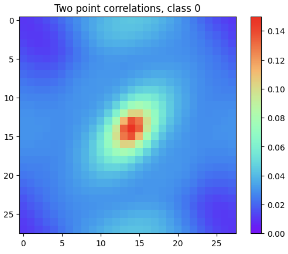
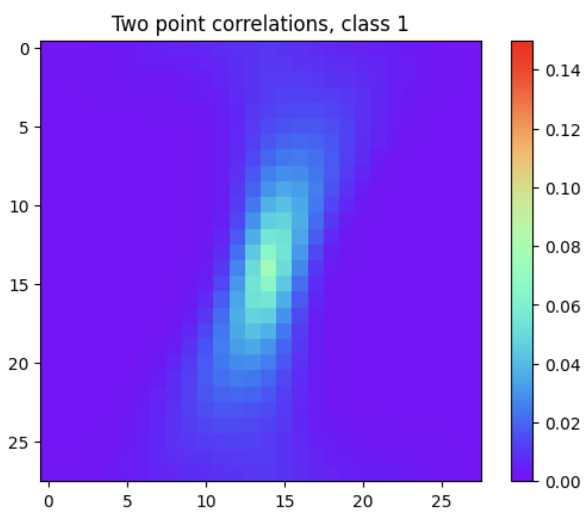
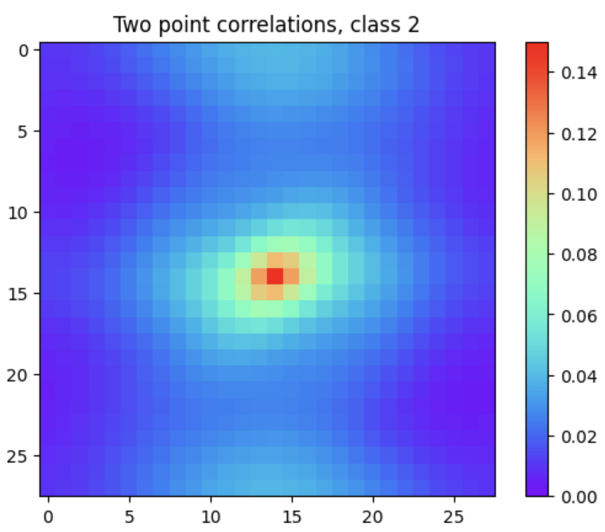
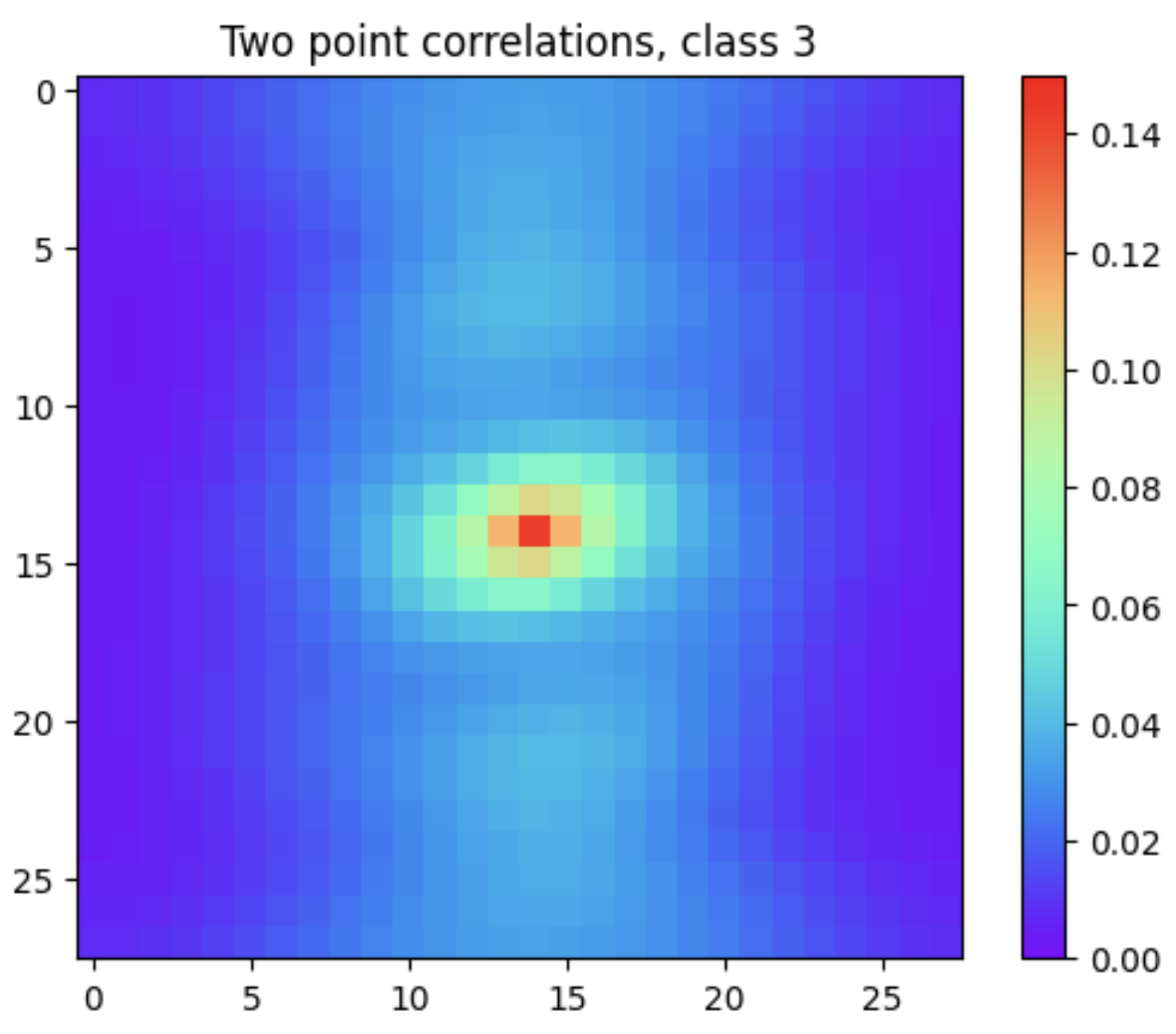
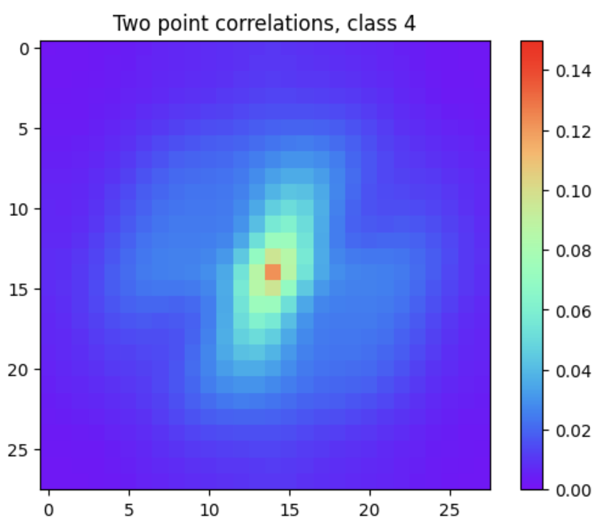
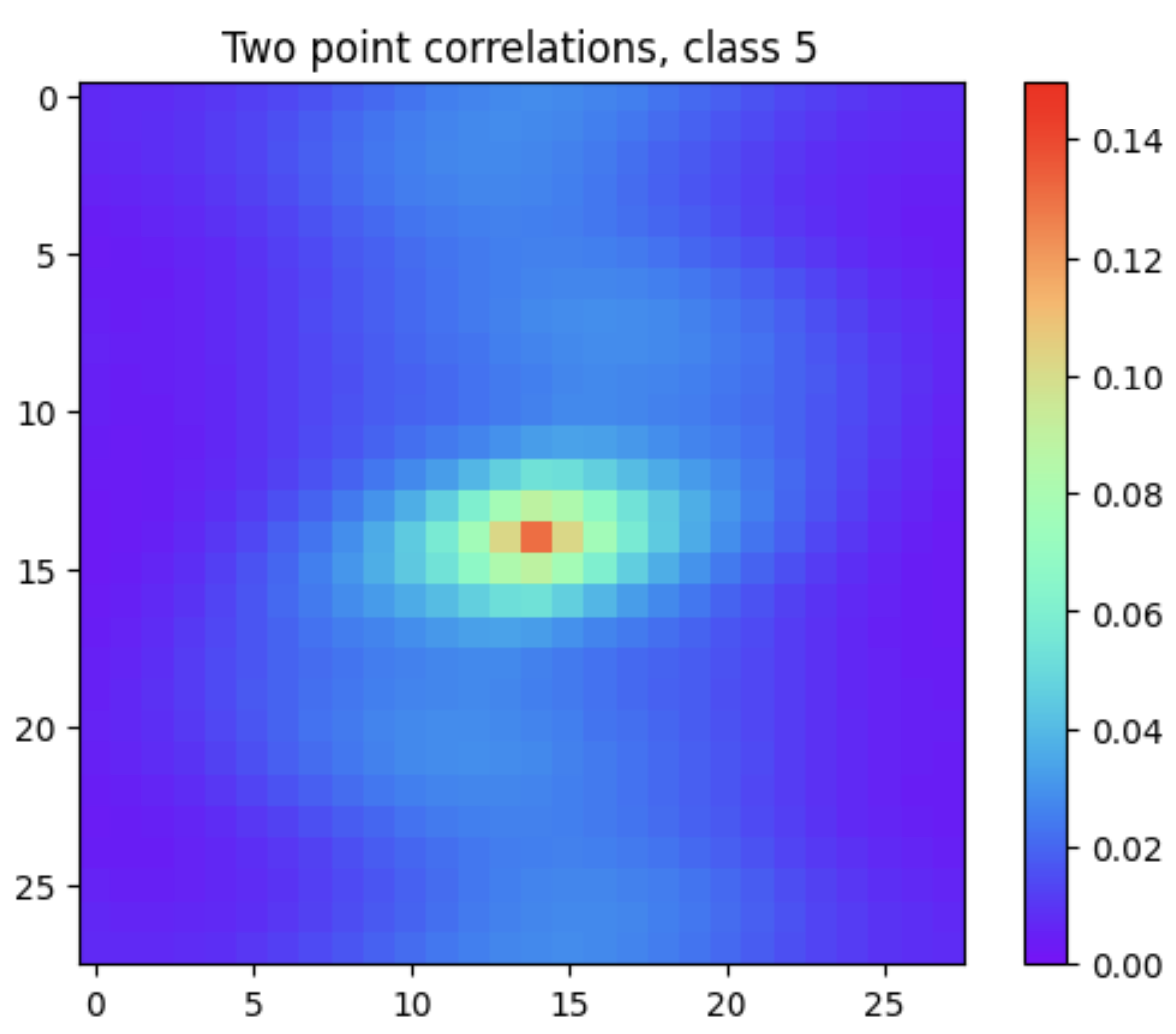
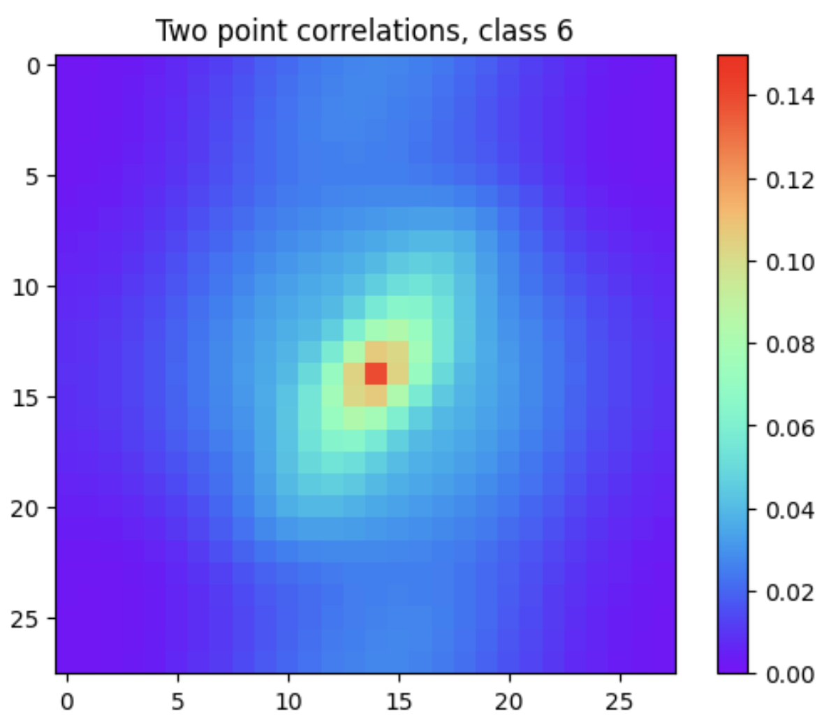
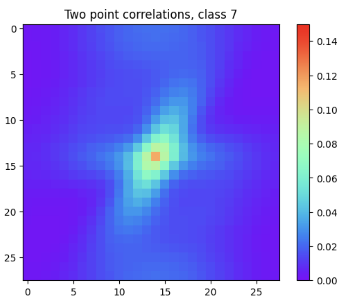
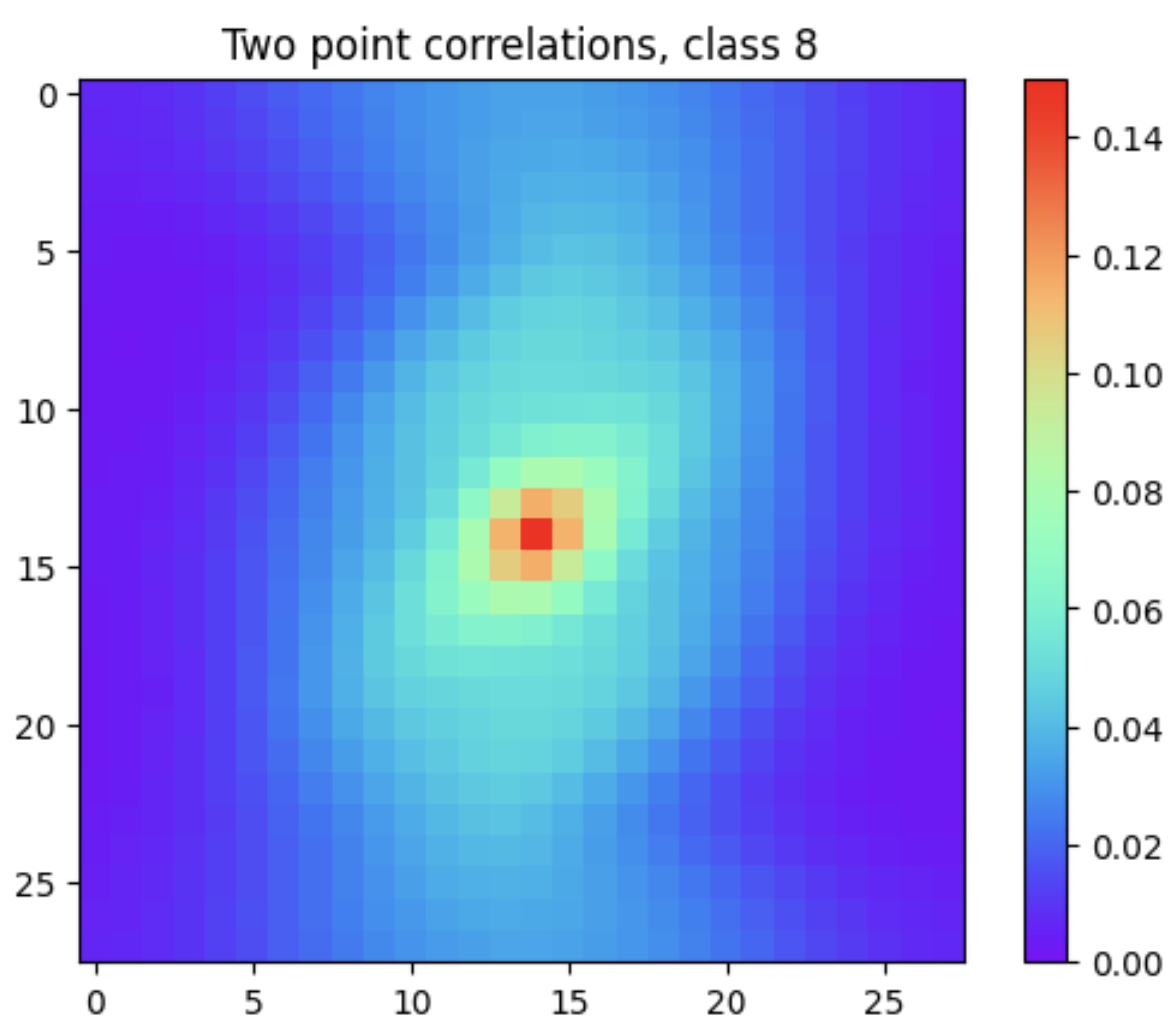
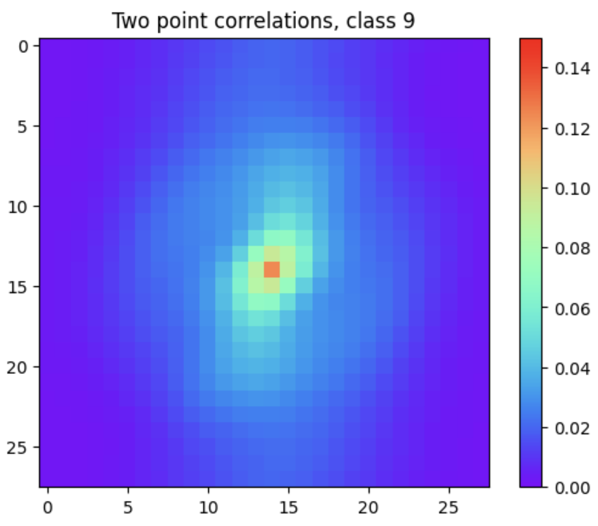
Figure 10: 2-Point Probability Plots

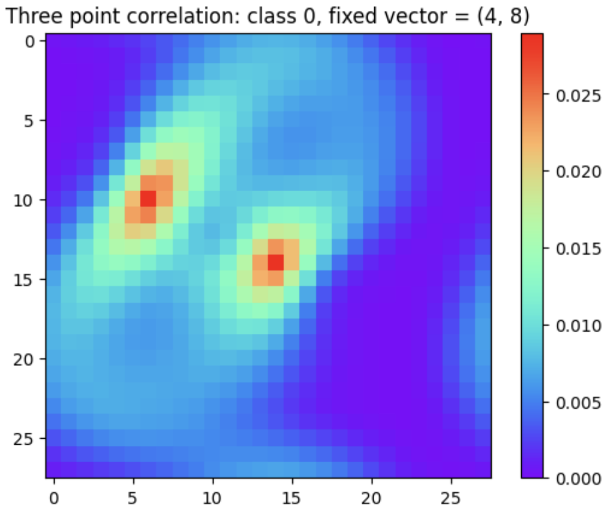
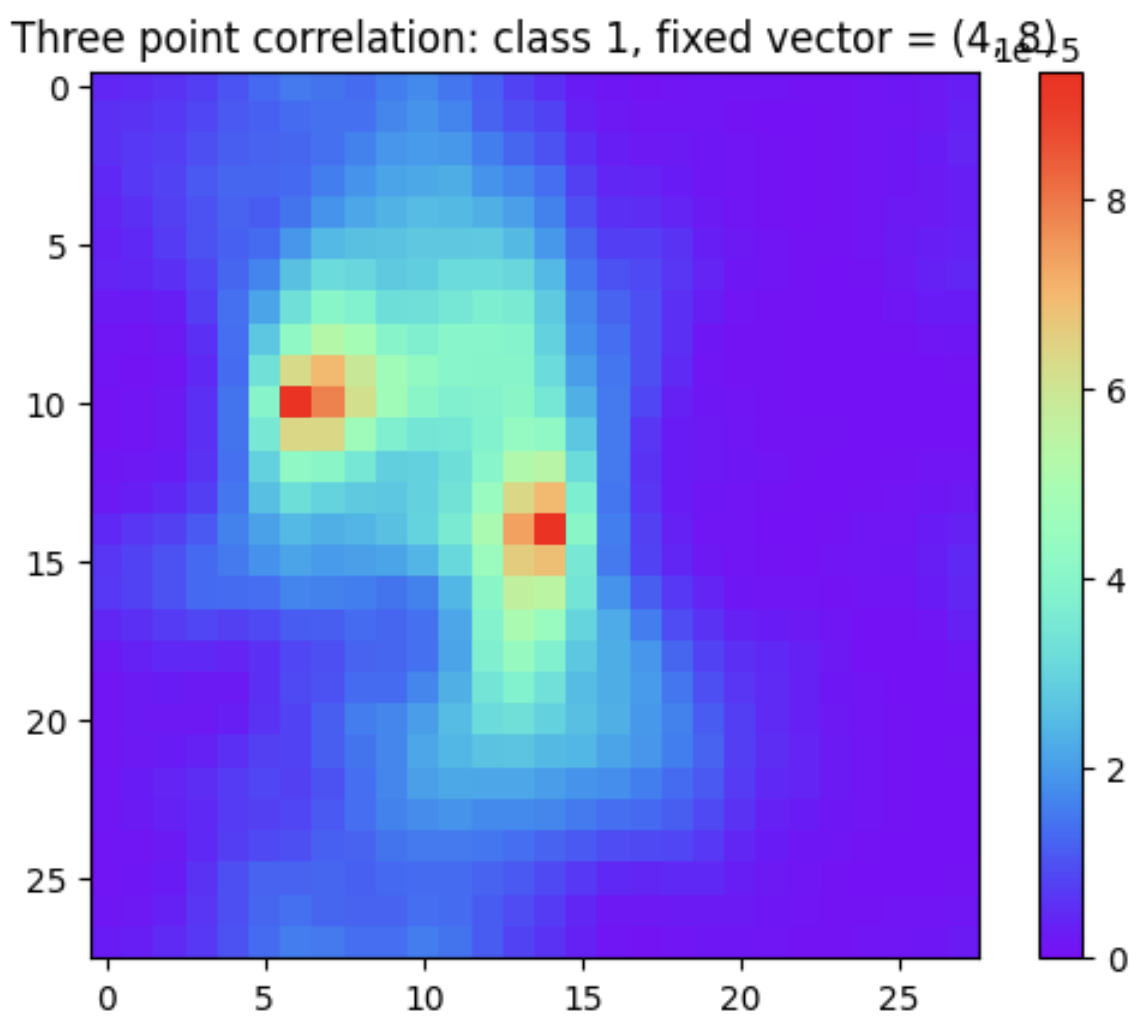
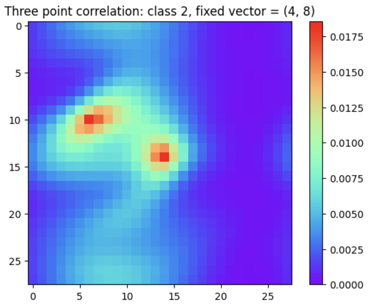
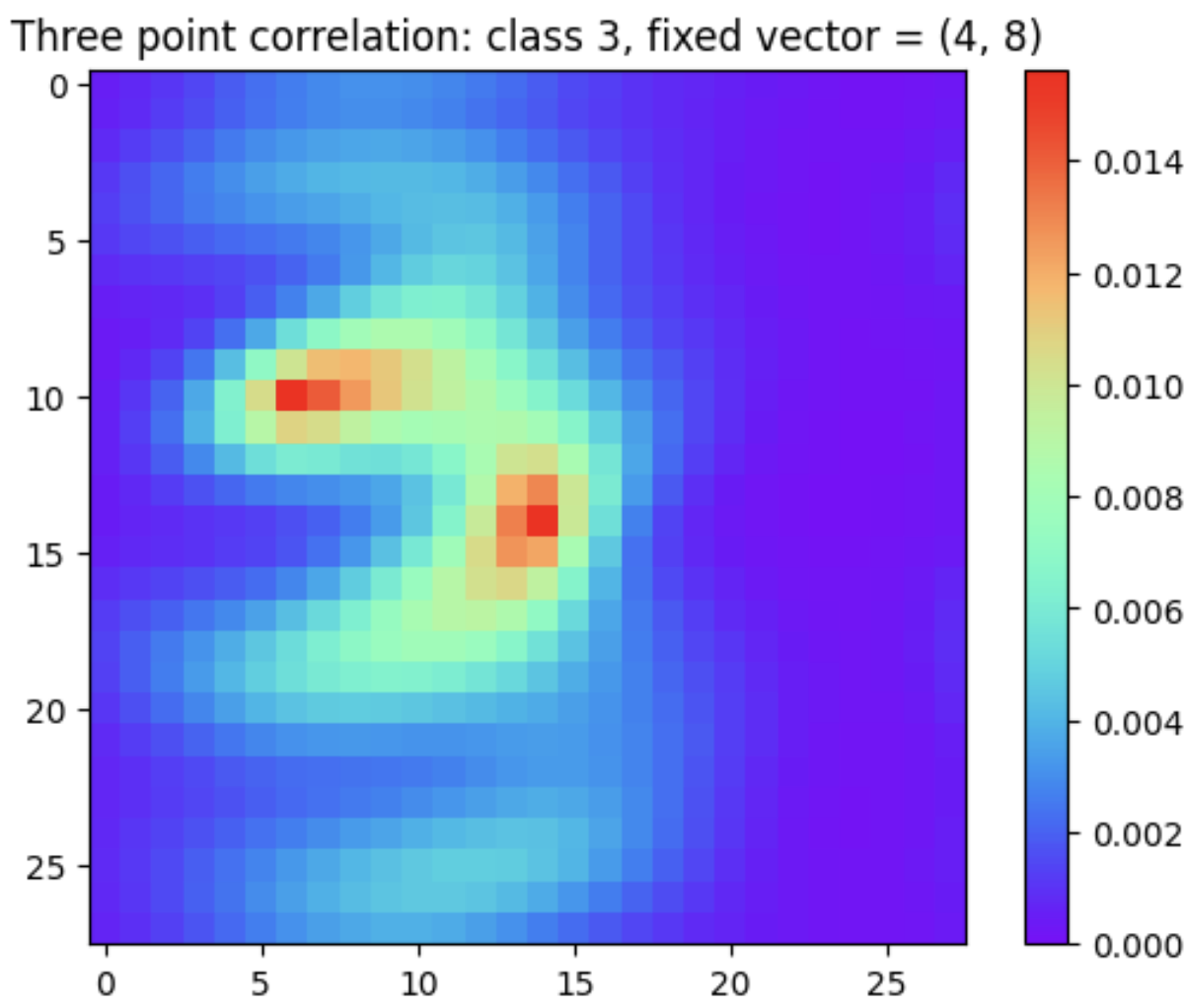
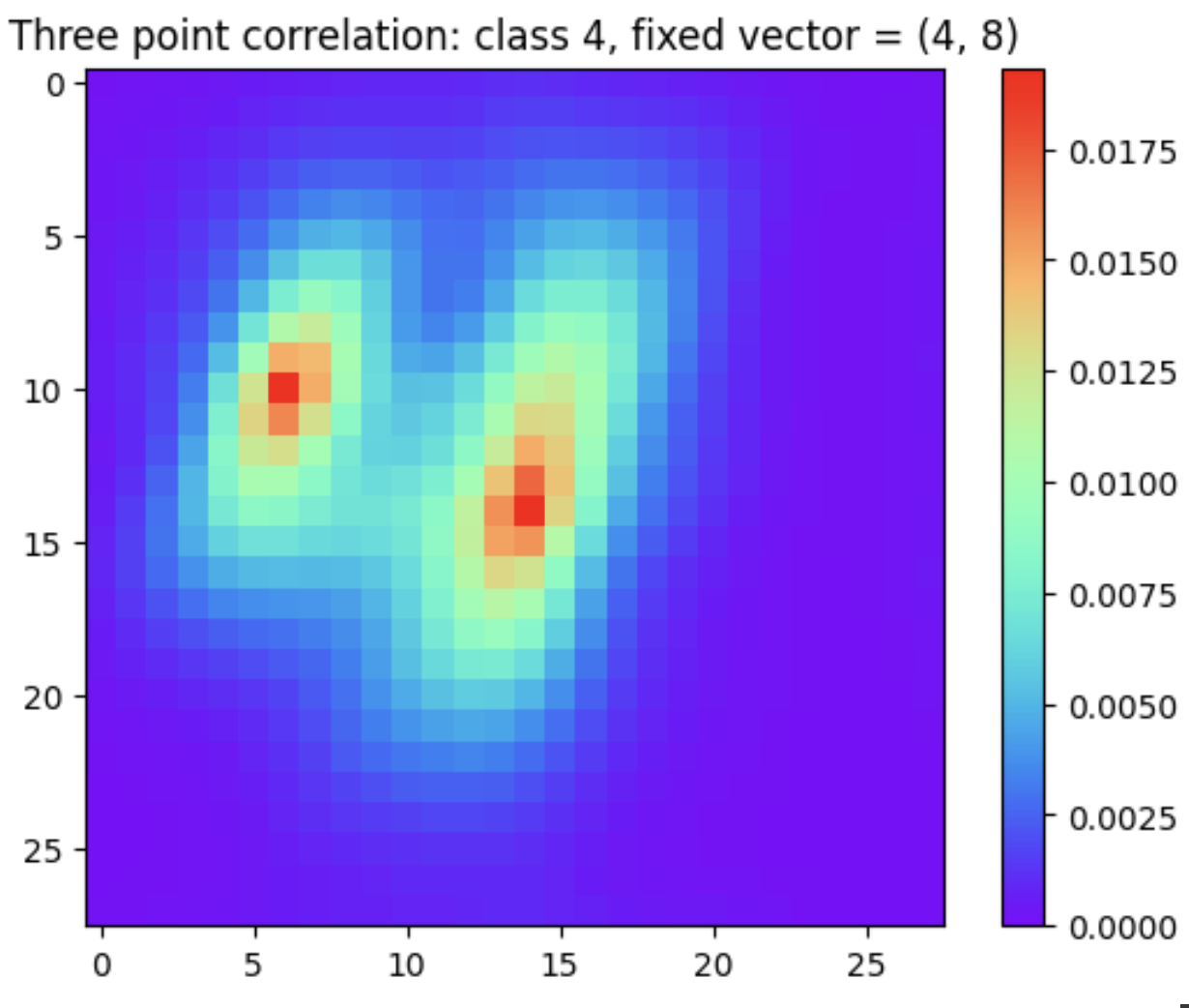
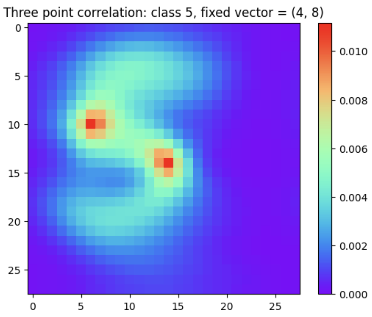
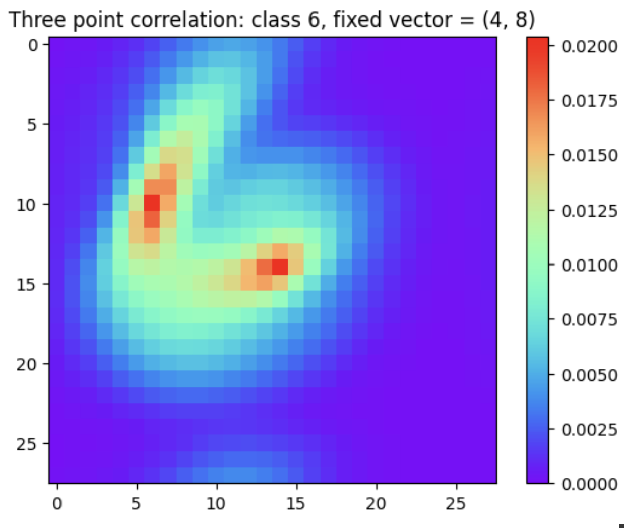
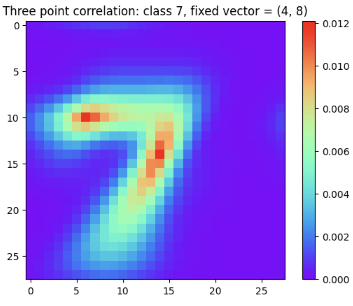
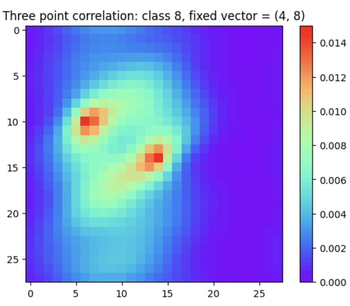
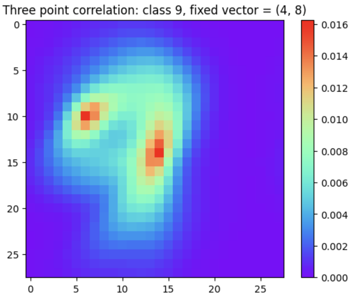
Figure 11: 3-Point Probability Plots

Figure 11 displays the $3$-point correlations for each class of numerals with the shift from pixel $x_{i,j}$, set to ${\bf k}=(4,8)$. These, and other plots implementing the same formula (with different shift pixels ${\bf k}$), provide evidence that higher order correlation functions of the kind discussed briefly in section 3, are sufficient for distinguishing distinct classes of numerals in the MNIST dataset. It is reasonable, we believe, to expect similar results from the other datasets mentioned listed in section 4. However, the second question remains: Can one show that, as a matter of fact, image recognitions DNNs are indeed finding such higher order correlations. How are these correlation functions being realized? The next section provides some evidence that, in fact, DNNs are finding such correlations and offers a suggestion of how (at least theoretically) they are able to do so.

5.2 Learning Higher Order Correlations

A recent paper entitled “Neural Networks Trained with SGD Learn Distributions of Increasing Complexity” Refinetti_Learning_distrib proposes what they call the Distributional Simplicity Bias (DSB):

“A parametric model trained on a classification task using SGD discriminates its inputs using increasingly higher-order input statistics as training progresses.” (Refinetti_Learning_distrib, , p. 2)

They motivate this principle by considering a simple/toy model of a single perceptron that is trained to distinguish between two types of data points that reside in two distinct rectangles in a plane. See figure 12.

Figure 12: Rectangular Data and Decision Boundaries (Refinetti_Learning_distrib, , p. 4)

The data ${\bf x}=(x^{i})_{i\leq D}$ are split into the two equally probable classes and are given labels $y_{i}$ with $i=\pm 1$. As one can see, the optimal decision boundary between the two classes is a line (dot-dashed) parallel to the $x_{2}$-axis that they call the “oracle.” (Refinetti_Learning_distrib, , p. 4). The perceptron’s output is given by:

$$\hat{y}-\sigma{\lambda},\quad\mbox{for}\quad\lambda\equiv w_{i}x^{i}/\sqrt{D},$$ (17)

with the weight vector $w_{i}$ and a nonlinear (sigmoid) activation function $\sigma$. The penalty during training is given by the square loss:

$$l(\lambda,y)=(\sigma(\lambda)-y)^{2}.$$

The perceptron is initialized with weights drawn from a Gaussian with variance 1 and then trained on a test set. They examine how the weight vector evolves during SGD with the given loss function. That is, they study the gradient flow:

$$\dot{w_{i}}=\eta\mathbb{E}(\sigma(\lambda-y)\sigma^{\prime}(\lambda)x^{i},$$ (18)

with fixed learning rate $\eta>0$. Here $\mathbb{E}$ is an average over the data distribution. (Refinetti_Learning_distrib, , p. 4). They do a Taylor expansion of activation function around $\lambda=0$:

$$\sigma(\lambda)=\sum_{k=0}^{\infty}\beta_{k}\lambda^{k}.$$

This gives the derivative

$$\sigma^{\prime}(\lambda)\sum_{k=0}^{\infty}\tilde{\beta}_{k+1}\lambda^{k-1},$$

with $\tilde{\beta_{k}}=k\beta_{k}=k\sigma^{(k)}(\lambda)|_{\lambda=0}.$

When entered into the gradient equation (18) this yields:

$$\frac{1}{\eta}\dot{w_{i}}=\sum_{k=0}^{\infty}\mathbb{E}\lambda^{k}x^{i}(\gamma_{k}-\tilde{\beta}_{k+1}y),$$ (19)

with $\tilde{\beta}_{k}$ and $\gamma_{k}$ constants from the Taylor expansion. This allows them to look at the zeroth order through third order components of the gradient flow (18) of the perceptron weight as it is trained.

They show that at zeroth order the “weight converges in direction” as

$$w_{i}^{0}\propto m^{i}\equiv\kappa_{+}^{i}-\kappa_{-}^{i}.$$

This is the difference between the means of each class, $\kappa_{\pm}^{i}=\mathbb{E}_{\pm}x^{i}.$ The idea here is that under training of this simple model, the decision boundary between the two classes rotates in the direction of the (curved) arrow in figure 12. At this zeroth order, the decision boundary moves to a line (yellow) splitting the means of the two rectangular classes.

At first order, the gradient of $w_{i}$ depends upon the second moments of the (data) inputs taking into consideration the difference between the “within class” variances and the variances “between classes.” This further rotates the decision boundary to the right and yields the classifier $w_{i}^{(1)}$, known in statistics as “Fisher’s linear discriminant.” (Refinetti_Learning_distrib, , p. 4) In figure 12, this is the green line.

Next, the second order term in the expansion contributes nothing to the gradient flow as it would involve the third moment which in this case is equal to zero because of symmetry in the data. As a result, the second order term in the perturbation expansion of the gradient flow does not improve upon the first order term.

Finally, the third order involves the fourth moments: $\kappa^{ijkl}$. As with the second moments, they decompose the fourth moment into a “between-class” fourth moment and a “within-class” fourth moment. Without going into the details, this allows them to express the fourth moments in terms of contributions from a “within-class” fourth order cumulant and contributions from the mean and second moments. At this order the expansion finally takes into consideration some non-Gaussian correlational information that is present in the dataset. For the current problem, this information rotates the decision boundary (now the purple line) even closer to the “oracle.”

The procedure here strongly resembles that employed in the so-called $\epsilon$-expansion in quantum field theory. There one aims to determine $N$-point correlations (Greens functions) via a perturbation expansion around a zeroth order Gaussian field.. In that context the calculations are facilitated by the use of Feynman diagrams which allow for the (relatively) easy summation of cumulants of higher orders.

This single perceptron model is an extremely simple toy model. It allows one to explicitly demonstrate how the consideration of higher order correlations can improve classification. But, of course, this model is not really learning increasingly complex functions. As Refinetti et al., note “its decision boundary remains a straight line.” (Refinetti_Learning_distrib, , p. 5) Nevertheless, as noted, the direction of the weight vector $w_{i}$,

and hence its decision boundary, first only depends on the means of each class, …, then on their mean and covariance, …, and finally also on higher-order cumulants, …, yielding increasingly accurate predictors. (Refinetti_Learning_distrib, , p. 5)

As further evidence for their “distribution centric” (Refinetti_Learning_distrib, , p. 6) point of view, these authors train neural networks with different architectures on various approximate “clones” of the CIFAR dataset. These clones are designed to have the same mean and covariance as the images in CIFAR, but also differ by progressively including higher order cumulants. (Refinetti_Learning_distrib, , pp. 6–8) The results, while somewhat preliminary, provide further evidence that the neural networks are learning distributions of increasing complexity after having learned the first and second order (Gaussian) correlational statistics.

Our goal in this section has been to provide some evidence in favor of the hypothesis that DNNs are successful at certain tasks (specifically, but not exclusively, image recognition tasks) because they implement something like the correlation function methodology described in section 3. This evidence is reflected in arguments for what Refinetti et al. call the “distributional simplicity bias.” It explicitly appeals to the stochastic gradient descent algorithm (SGD) and aims to show that the algorithm is driven by progressively examining higher order dataset statistics. As noted, the idea here is similar to those developed in the context of quantum field theoretic perturbative calculations of $N$-point correlation (Green’s) functions. The idea there being that all of the information about a quantum field is to be found in those functions. In analogy, we believe that being able to determine $N$-point correlation functions of image datasets for $N>2$, will provide information sufficient for the successes of DNNs on image recognition tasks. As noted in section 3 one way to conceptualize this is the following: DNNs, in determining higher order correlation functions, are finding statistical representatives (RVEs) that uniquely distinguish classes in a given dataset.

6 Conclusion

We would like to stress that understanding the successes of DNNs on various tasks requires a focus on facts about the world. These worldly facts are responsible for robust statistical properties that are present in the datasets upon which the DNNs are trained. The workings of DNNs will remain obscure and opaque if one only looks “under the hood” and ignores these robust, universal, features of the datasets. Furthermore, we believe that these statistical features present in the datasets are what drive the dynamics of weight updating.

In addition, we have argued that DNNs are actually implementing a well-understood methodology (important for any field that aims to explain continuum scale behavior of complex systems) that privileges correlational structures at mesoscales. middleway In the context of image recognition, the lowest (fundamental) scale corresponds to features of individual pixels such as their luminance, their weighted color (RGB) values, etc. In analogy with many-body physical systems, the “continuum” scale behavior of images is their (correct) label—whether the image is that of a dog, a cat, …. As in the physical examples, the most important features or quantities for identifying the images as members of a given class are functions that represent correlational structures in the images at mesoscales. And, just as in the physical examples, these correlations are hidden at the smallest pixel scale. The discovery of these correlational features allows for successful identification of an image as a member of a specific class.

Our focus on correlational structures in datasets also highlights differences between understanding contemporary deep learning and the theoretical perspective of statistical learning theory. As we noted, DNNs can successfully generalize to test sets upon training, despite commonly employing more parameters than the data points on which they are trained. This is contrary suggestions from SLT and, for that matter, conventional informal statistical wisdom about overfitting. We suggested that part of the reason for this is a mismatch between the assumptions made in SLT and the empirical features of the data on which they are trained. SLT provides worst case bounds on expected performance on a test set without any assumptions concerning the probability distributions characterizing the data. However, as we have emphasized, real world data consisting of images is governed by very specific kinds of probability distributions. DNNs, we suggest, operate so as to learn certain features of these probability distributions, particularly those having to do with higher order correlations. By contrast, for arbitrary probability distributions, higher order correlation functions may not exist or may be uninformative. Moreover, in constructing and training DNNs that classify well, what matters is not worse case behavior but something more like typical or attainable behavior.

Another way of expressing this point is to note that, although the collections of images on which DNNs are trained have very high dimensionality, there is a great deal of evidence that (as one might expect) the effective number of dimensions that the DNNs employ in classifying data is many orders of magnitude smaller. This reflects the fact that there is a great deal of redundancy in real life images when these are viewed at the level of individual pixels and the task is one of sorting them into rather coarse-grained categories (“dog” vs. “cat”). The presence of scale invariances and power law distributions in the characterization of images, detailed above, is one facet of such redundancy. Note again, that there is nothing a priori about this—one can certainly imagine a collection of pixels that does not have this kind of redundant structure. There, the exact luminance levels of pixels in comparison with other arbitrarily chosen pixels might be critical for how the collection is classified. Presumably, however, collections of pixels without such redundant structure would not be recognizable by us as images of anything—they would look like noise. As Ruderman’s work shows, images in the sense of scenes composed of objects recognizable by us, have very different structures. When we train a DNN to classify in accordance with the classifications we make, we train it to pay attention to these structures. Another observation: As noted in section 2, real images have the feature that pixels that are close by in physical distance are generally similar in luminance. One can think of this as a kind of smoothness condition—pixel luminances do not generally vary wildly over short distances. This smoothness condition is another “worldly condition” that characterizes real life images.

It is tempting to make the following connection: As Martin and Mahoney Martin_Mahoney_rmt (and others) have shown, stochastic gradient descent implements “self-regularization”. That is, it selects functions that have low norm. Such functions are also relatively smooth—they don’t exhibit large changes over small distances. In this respect they are well matched to the smoothness condition satisfied by real life images. One may then conjecture that such self-regularization selects for functions that track these features, thereby helping to explain why SGD leads to results that “work” for images. If this is correct, one would expect that DNNs trained with SGD would work less well with structures that do not satisfy smoothness conditions and this in fact is what is found. simplicity_bias

Summing up, one can contrast two different approaches to understanding the generalizing abilities of DNNs. The first, characteristic of SLT (and other similar approaches) focuses on the class of functions that are available to classify images but does not assume that the images themselves have any particular structure. This approach cannot explain why DNNs successfully generalize. The second approach focuses on specific features of the images themselves, including the presence in them of higher order correlational structures. This approach explains successful generalization in terms of the ability of DNNs to exploit these structures. This suggests the following research program: Look for the features of the images themselves that can support successful generalization to new cases.

References

- (1) M. Baniassadi, S. Ahzi, H. Garmestani, D. Ruch, and Y. Remond. New approximate solution for -point correlation functions for heterogeneous materials. Journal of the Mechanics and Physics of Solids, 60:104–199, 2012.
- (2) Robert W. Batterman. A Middle Way: A Non-Fundamental Approach to Many-Body Physics. Oxford University Press, 2021.
- (3) Mikhail Belkin, Daniel Hsu, Syuan Ma, and Soumik Mandal. Reconciling modern machine-learning practice and the classical bias-variance trade-off. PNAS, 116(32):15849–15854, 2019.
- (4) Christopher M. Bishop. Pattern Recognition and Machine Learning. Springer, New York, 2006.
- (5) Florian J. Boge. Two dimensions of opacity and the deep learning predicament. Minds and Machines, 32:43–75, 2022.
- (6) Harold W. Chalkley, Jerome Cornfield, and Helen Park. A method for estimating volume-surface ratios. Science, 110:295–298, 1949.
- (7) Kathleen Creel. Transparency in complex computational systems. Philosophy of Science, 87(4):568–589, 2020.
- (8) P. Debeye, H. R. Anderson Jr., and H. Brumberger. Scattering by an inhomegeneous solid. ii. the correlation function and its application. Journal of Applied Physics, 28(679–683), 1957.
- (9) Eamon Duede. The representational status of deep learning models. arXiv:2303.12032v2, 2025.
- (10) Dieter Forster. Hydrodynamic Fluctuations, Broken Symmetry, and Correlation Functions. Advanced Book Classics. Perseus Books, 1990.
- (11) Nigel Goldenfeld. Lectures on Phase Transitions and the Renormalization Group. Number 85 in Frontiers in Physics. Addison-Wesley, Reading, Massachusetts, 1992.
- (12) Sebastian Goldt, Marc Mézard, Florent Krzakala, and Lenka Zdeborová. Modelling the influence of data structure on learning in neural networks: The hiddn manifold model. arXiv:1909.11500v4, 2020.
- (13) A. N. Gorban and I. Y. Tyukin. Blessing of dimensionality: Mathematical foundations of the statistical physics of data. Philosophical Transactions of the Royal Society A: Mathematical, Physical and Engineering Sciences, 376(20170237), 2018.
- (14) Leo P. Kadanoff. Theories of matter: Infinities and renormalization. In Robert W. Batterman, editor, The Oxford Handbook of Philosophy of Physics, chapter Four, pages 141–188. Oxford University Press, 2013.
- (15) Leo P. Kadanoff and Paul C. Martin. Hydrodynamic equations and correlation functions. Annals of Physics, 24:419–469, 1963.
- (16) Kenji Kawaguchi, Leslie Pack Kaelbling, and Yoshua Bengio. Generalization in deep learning. arXiv:1710.05468, 2023.
- (17) Noam Levi and Yaron Oz. The underlying scaling laws and universal structure of complex datasets. arXiv:2306.14975v3, 2024.
- (18) Henry W. Lin, Max Tegmark, and David Rolnick. Why does deep and cheap lerning work so well? Journal of Statistical Physics, 168:1223–1247, 2017.
- (19) Charles H. Martin and Michael W. Mahoney. Implicit self-regularization in deep neural networks: Evidence from random matrix theory and implications for learning. CoRR, abs/1810.01075, 2018.
- (20) Maria Refinetti, Alessandro Ingrosso, and Sebastian Goldt. Neural networks trained with SGD learn distributions of increasing complexity. arXiv:2211.11567v2, 2023.
- (21) Daniel L. Ruderman. Origins of scaling in natural images. Vision Research, 37(23):3385–3398, 1997.
- (22) Daniel L. Ruderman and William Bialek. Statistics of natural images: Scaling in the woods. Physical Review Letters, 73(6):814–817, 1994.
- (23) Emily Sullivan. Understanding from machine learning models. The British Journal for the Philosophy of Science, 73(1):109–133, 2022.
- (24) Emily Sullivan. Do machine learning models represent their targets? Philosophy of Science, 91(5):1445–1455, 2024.
- (25) Damien Teney, Liangze Jian, Florin Gogianu Bitdefender, and Eshan Abbasnejad. Do we always need the simplicity bias? looking for optimal inductive biases in the wild. arXiv:2503.10065v1, 2025.
- (26) Salvatore Torquato. Random Heterogeneous Materials: Microstructure and Macroscopic Properties. Springer, New York, 2002.
- (27) Andrew Gordon Wilson. Deep learning is not so mysterious or different. Proceedings of the International Conference on Machine Learning, 2025.
- (28) Kenneth G. Wilson and J. Kogut. The renormalization group and the expansion. Physics Reports, 12(2):75–199, 1974.
- (29) D. H. Wolpert and W. G. Macready. No free lunch theorems for optimization. IEEE Transactions on Evolutionay Computation, 1:67–82, 1997.
- (30) Zitong Yang, Yaodong Yu, Chong You, Jacob Steinhardt, and Yi Ma. Rethinking bias-variance trade-off for generalization of neural networks. Proceedings of the International Conference on Machine Learning, 2020.
- (31) Chiyuan Zhang, Samy Bengio, Moritz Hardt, Benjamin Recht, and Oriol Vinyals. Understanding deep learning requries re-thinking generalzition. ArXiv:1611.03530v2, 2017.