CSV-Decode: Certifiable Sub-Vocabulary Decoding for Efficient Large Language Model Inference

Abstract

Large language models face significant computational bottlenecks during inference due to the expensive output layer computation over large vocabularies. We present CSV-Decode, a novel approach that uses geometric upper bounds to construct small sub-vocabularies for each decoding step, enabling efficient sparse computation while maintaining dual correctness guarantees: exact top-$k$ certification and $\varepsilon$-certified softmax approximations. Our method clusters vocabulary embeddings offline and uses centroid-plus-radius bounds to identify which tokens can be safely omitted from computation. We provide a complete system implementation with sparse GEMV kernels, multi-GPU sharding, and CUDA Graph optimization. Experimental results demonstrate significant speedup over full vocabulary decoding while maintaining distributional guarantees and low fallback rates. Our code implementation available at https://github.com/FastLM/CSV-Decode.

I Introduction

Large Language Models (LLMs) have revolutionized natural language processing, achieving state-of-the-art performance across diverse tasks including text generation, question answering, and code synthesis [vaswani2017attention, touvron2023llama, jiang2023mistral]. However, the deployment of these models in production environments faces significant computational challenges, particularly during the inference phase. The rapid growth in model size and vocabulary dimensions—with orders-of-magnitude increases over the past few years—has created substantial bottlenecks that limit the practical applicability of LLMs in real-world scenarios.

The core challenge lies in the fundamental tension between model capability and computational efficiency. While larger vocabularies enable better multilingual support and more precise tokenization, they dramatically increase the computational cost of each inference step. This creates a critical scalability issue for real-world deployments, where latency and energy consumption directly impact user experience and operational costs.

I-A The Output Layer Bottleneck

The most computationally expensive component of LLM inference is the output layer computation, which transforms the final hidden representation into probability distributions over the vocabulary. For a model with vocabulary size $V$ and hidden dimension $d$, each decoding step requires computing logits $\ell_{i}(t)=\left\langle W_{i},\,h_{t}\right\rangle+b_{i}$ for all tokens $i\in[V]$, where $W\in\mathbb{R}^{V\times d}$ represents the output layer weight matrix, $b\in\mathbb{R}^{V}$ is the bias vector, and $h_{t}\in\mathbb{R}^{d}$ is the hidden state at decoding step $t$. This matrix-vector product operation has computational complexity $\mathcal{O}(Vd)$, which scales linearly with vocabulary size.

Modern LLMs vary significantly in vocabulary size, with recent foundation models typically employing 32K–256K tokens [touvron2023llama, jiang2023mistral]. Table I summarizes representative vocabulary sizes across major model families. Hidden dimensions typically range between 4,096 and 8,192. This results in output layer weight matrices of substantial size (e.g., 128K$\times$4K to 256K$\times$8K), making the output layer computation the dominant bottleneck in inference pipelines [grave2017efficient]. For example, in GPT-3 with $V=50,257$ tokens and $d=12,288$ hidden dimensions, the output layer contains over 600 million parameters. The matrix-vector product $V\times d$ requires approximately $6.17\times 10^{8}$ multiply-adds $\approx 1.23\times 10^{9}$ FLOPs/token (counting 1 mul + 1 add = 2 FLOPs), not $10^{12}$ as often misclaimed, for the output layer computation alone.

TABLE I: Vocabulary Sizes of Some Modern LLMs

Model Family	Organization	Vocabulary Size
Phi-3	Microsoft	32,000
Mistral-7B	Mistral AI	32,768
DeepSeek-Coder	DeepSeek	50,264
Yi-34B	01.AI	64,000
Llama-3	Meta	128,256
Mistral-Large	Mistral AI	131,072
Qwen2.5	Alibaba	151,552
Gemma2	Google	256,000

I-B Challenges in Existing Approaches

Current approaches to address the output layer bottleneck fall into several categories, each with significant limitations:

Adaptive Softmax: Grave et al. [grave2017efficient] proposed adaptive softmax, which clusters frequent tokens and uses different computation strategies for different clusters. While effective, this approach requires retraining the model and may not generalize well to different domains or tasks. Additionally, the clustering is static and cannot adapt to dynamic patterns in the input.

Hierarchical Softmax: Mikolov et al. [mikolov2013efficient] introduced hierarchical softmax in the context of word2vec, using a binary tree structure to reduce complexity to $\mathcal{O}(\log V)$. Here we follow the same HSoftmax structure principle, but it requires significant architectural changes to the model. The tree structure must be carefully designed and may not capture the semantic relationships between tokens effectively.

Approximate Nearest Neighbor Methods: Various approximate methods have been proposed, including sampling-based approaches [graham2014sparse] and quantization techniques [fan2020reducing]. However, these methods sacrifice correctness guarantees, which is problematic for applications requiring precise probability distributions or exact top-$k$ rankings.

Speculative Decoding: Recent work on speculative decoding [leviathan2023fast] uses smaller models to predict likely tokens, but focuses on reducing the number of forward passes rather than addressing the output layer computation directly.

I-C The CSV-Decode Insight

Our key insight is that for most decoding steps, only a small subset of the vocabulary actually contributes meaningfully to the final output distribution. This observation is both intuitive and empirically verifiable: given a specific context, most vocabulary tokens are semantically irrelevant and have negligible probability mass. This observation is based on several factors:

1. Semantic Clustering: Vocabulary embeddings naturally cluster in the embedding space, with semantically similar tokens located close to each other.

2. Context Sensitivity: The hidden state $h_{t}$ at each step is context-dependent, and only tokens whose embeddings align well with the current context will have high logits.

3. Top-k Dominance: In most applications, only the top-$k$ tokens (where $k$ is typically 10-100) are actually used for sampling or ranking, making the remaining tokens irrelevant.

By leveraging geometric upper bounds derived from clustered vocabulary embeddings, we can identify which tokens can be safely omitted from computation without affecting the final results. The key innovation is that we can prove mathematically that certain tokens cannot enter the top-$k$ results or significantly affect the probability distribution, allowing us to skip their computation entirely. This approach maintains provable correctness guarantees—exact for top-$k$ tasks and $\varepsilon$-bounded for softmax distributions—while enabling substantial computational savings that scale with vocabulary size.

I-D Main Contributions

This paper presents CSV-Decode, a novel approach for efficient large language model inference that addresses the output layer bottleneck through geometric reasoning and provable bounds. Our main contributions are:

1. Geometric Upper Bounds: We develop a novel approach using centroid-plus-radius bounds to construct provably correct sub-vocabularies for each decoding step. This method clusters vocabulary embeddings offline and uses Cauchy-Schwarz inequality to derive tight upper bounds on logits for entire clusters.

2. Exact Certification: We provide two certification mechanisms: (1) exact top-$k$ certification that guarantees no token outside the sub-vocabulary can enter the top-$k$ set, and (2) $\varepsilon$-certified softmax approximation with bounded total variation distance.

3. Adaptive Online Algorithm: We design an efficient online algorithm that dynamically expands sub-vocabularies based on certification criteria, ensuring optimal trade-offs between computational efficiency and accuracy guarantees.

4. System Implementation: We provide a complete system implementation featuring optimized sparse GEMV kernels, multi-GPU sharding with NCCL communication, CUDA Graph integration for reduced launch overhead, and intelligent fallback mechanisms.

5. Comprehensive Evaluation: We conduct extensive experiments on multiple models (Llama-2, Mistral, CodeLlama) and datasets (Wikitext-103, HumanEval, MT-Bench) demonstrating 2-3x speedup while maintaining high quality and low fallback rates.

The computational complexity reduction follows an amortized model accounting for various cost components:

$$T_{\text{csv}}\approx\alpha\cdot(Cd)+\beta\cdot(|S_{t}|d)+\gamma$$ (1)

where $|S_{t}|$ is the dynamically determined sub-vocabulary size, $\alpha$ accounts for bound computation overhead, $\beta$ represents sparse GEMV costs, and $\gamma$ includes constant factors like heap maintenance, cluster opening gather operations, bias access, and softmax normalization. For large vocabulary scenarios where $Cd$ becomes significant, caching and bandwidth effects make the relationship nonlinear. The empirical coefficients $\alpha$, $\beta$, $\gamma$ are provided in the appendix with GPU-specific fitting results. The architecture achieves optimal performance when the bound tightness ratio $\xi=\frac{\max_{i\in S_{t}}\ell_{i}-\min_{i\in S_{t}}\ell_{i}}{U_{\max}-\min_{i\in S_{t}}\ell_{i}}$ approaches 1.0, indicating tight geometric bounds that minimize unnecessary token inclusion.

I-E Paper Organization

The remainder of this paper is organized as follows. Section II provides background on output layer computation and reviews related work. Section III presents the CSV-Decode methodology, including geometric bounds and certification algorithms. Section IV describes the system design and implementation details. Section V presents comprehensive experimental evaluation. Section VI discusses limitations and future work. Section VII concludes the paper.

II Background and Related Work

II-A Output Layer Computation in LLMs

The output layer of transformer-based language models serves as the final transformation layer, converting the contextualized hidden representations into probability distributions over the vocabulary. This process involves two main steps: logit computation and probability normalization.

II-A1 Logit Computation

For each decoding step $t$, the model computes logits $\ell_{i}(t)$ for all tokens $i\in[V]$ in the vocabulary:

$$\ell_{i}(t) =\left\langle W_{i},\,h_{t}\right\rangle+b_{i}$$ (2)

where $W\in\mathbb{R}^{V\times d}$ is the output weight matrix, $W_{i}\in\mathbb{R}^{d}$ represents the $i$-th row corresponding to token $i$, $h_{t}\in\mathbb{R}^{d}$ is the hidden state at step $t$, and $b\in\mathbb{R}^{V}$ is the bias vector. The matrix-vector product $\left\langle W_{i},\,h_{t}\right\rangle$ dominates the computational cost, requiring $\mathcal{O}(Vd)$ operations per decoding step.

II-A2 Probability Normalization

The logits are then converted to probabilities using the softmax function:

$$p_{i}(t) =\frac{e^{\ell_{i}(t)}}{\sum_{j=1}^{V}e^{\ell_{j}(t)}}=\frac{e^{\ell_{i}(t)}}{Z(t)}$$ (3)

where $Z(t)=\sum_{j=1}^{V}e^{\ell_{j}(t)}$ is the partition function. The softmax computation requires $\mathcal{O}(V)$ additional operations for computing $Z(t)$ and normalizing all probabilities.

II-A3 Computational Complexity Analysis

The total computational complexity of the output layer is $\mathcal{O}(Vd+V)=\mathcal{O}(Vd)$, where the matrix-vector product dominates for typical values of $d\gg 1$. For modern LLMs with vocabularies ranging from 32K to 256K tokens and hidden dimensions of 4,096-8,192 [touvron2023llama, jiang2023mistral], this results in billions of operations per decoding step.

II-B Related Work on Efficient Output Layer Computation

The output layer bottleneck has received significant attention from the research community, leading to various approaches to reduce computational complexity while maintaining model quality.

II-B1 Adaptive Softmax

Grave et al. [grave2017efficient] introduced adaptive softmax, which partitions the vocabulary into clusters based on token frequency and applies different computation strategies to each cluster. Frequent tokens are computed exactly, while infrequent tokens use approximations. This approach reduces the effective vocabulary size but requires retraining the model and may not generalize well to different domains or tasks.

The adaptive softmax approach has several limitations: (1) the clustering is static and cannot adapt to dynamic patterns, (2) it requires careful tuning of cluster sizes and thresholds, and (3) the performance gains are limited by the frequency distribution of tokens.

II-B2 Hierarchical Softmax

Mikolov et al. [mikolov2013efficient] proposed hierarchical softmax in word2vec, which organizes the vocabulary in a binary tree structure. Instead of computing probabilities for all tokens, the model navigates the tree by making binary decisions at each node, reducing complexity to $\mathcal{O}(\log V)$. However, this approach requires significant architectural changes and careful tree construction when adapted to modern transformer architectures.

The hierarchical softmax has several drawbacks: (1) the tree structure must be carefully designed to capture semantic relationships, (2) it may not work well for all types of models or tasks, and (3) the training process becomes more complex due to the tree structure.

II-B3 Sampling-Based Methods

Various sampling-based approaches have been proposed to approximate the softmax computation. Graham et al. [graham2014sparse] introduced sparse convolutional neural networks that use sampling to reduce computation. However, these methods sacrifice correctness guarantees and may introduce bias in the probability estimates.

Sampling-based methods face several challenges: (1) they require careful tuning of sampling strategies, (2) they may introduce variance in the results, and (3) they may not preserve the exact ranking of tokens, which is important for many applications.

II-B4 Quantization and Compression

Fan et al. [fan2020reducing] proposed reducing transformer depth on demand with structured dropout, which can reduce the size of the output layer. Various quantization techniques have also been applied to compress the output layer weights. However, these approaches may degrade model quality and require careful calibration.

II-B5 Speculative Decoding

Recent work on speculative decoding [leviathan2023fast] uses smaller models to predict likely tokens, reducing the effective search space for the main model. However, this approach focuses on reducing the number of forward passes rather than addressing the output layer computation directly. The recent work on parallel speculative decoding [liu2025pearl] addresses the mutual waiting problem in speculative decoding through pre-verify and post-verify strategies, achieving up to 4.43$\times$ speedup. However, PEARL is limited to speculative decoding scenarios requiring both draft and target models, suffers from GPU resource competition (89-99% performance retention), and provides no theoretical correctness guarantees. In contrast, CSV-Decode works universally with any LLM architecture, provides provable certification guarantees (exact top-$k$ and $\varepsilon$-bounded softmax), and achieves superior performance without resource competition issues.

II-B6 Complementary System-Level Optimizations

Beyond modifying the output layer itself, a parallel line of work targets end-to-end serving efficiency and long-context computation[liu2024efficientfoundation]. Memory-Keyed Attention (MKA) reduces the cost of long-context attention via hierarchical memory levels and recursive updates, enabling tighter compute and memory reuse without sacrificing quality [liu2025mka]. At the serving layer, TinyServe proposes query-aware cache selection that mitigates memory fragmentation and improves KV reuse under real-world, bursty query patterns [liu2025tinyserve]. PiKV further systematizes KV-cache management with a parallel, distributed design that co-optimizes routing, compression, and scheduling across multi-GPU/cluster deployments [liu2025pikv]. Orthogonal to attention and cache scheduling, LLMEasyQuant provides a scalable quantization toolkit that unifies static and online execution across single- and multi-node settings, improving throughput and memory footprint with minimal accuracy degradation [liu2024llmeasyquant].

II-C GPU Optimization for Sparse Computation

Modern GPUs provide specialized hardware for sparse matrix operations, including Tensor Cores and sparse tensor units. Our system leverages these capabilities through custom CUDA kernels and optimized memory access patterns.

II-C1 Multi-level Tiling

Recent work on multi-level tiling for sparse computation [dao2023flashattention2] has shown significant performance improvements by organizing computation in multiple levels of memory hierarchy. We apply similar techniques to our sparse GEMV kernels.

II-C2 CUDA Graph Integration

CUDA Graphs enable the capture of entire computation graphs, reducing kernel launch overhead in iterative algorithms like language model decoding. We use CUDA Graphs to optimize the CSV-Decode computation pipeline.

II-D Summary

While existing approaches provide various ways to reduce output layer computation, they either sacrifice correctness guarantees or require significant architectural changes. Our CSV-Decode approach addresses these limitations by providing rigorous correctness guarantees—exact top-$k$ certification and $\varepsilon$-bounded softmax approximation—while maintaining computational efficiency through geometric reasoning and provable bounds.

III CSV-Decode Methodology

This section presents the core methodology of CSV-Decode, including the geometric upper bounds, certification mechanisms, and the adaptive online algorithm. The approach is built on a simple but powerful geometric intuition: if we can bound the maximum possible logit value for all tokens in a cluster, we can safely prune entire clusters without computing individual token logits. We provide detailed mathematical derivations and proofs to establish the correctness guarantees of our approach.

III-A Geometric Upper Bounds

The foundation of CSV-Decode is the construction of tight upper bounds on logits for clusters of vocabulary embeddings. The central idea is straightforward: instead of computing logits for individual tokens, we first compute an upper bound for the maximum logit that any token in a cluster could achieve. If this upper bound is sufficiently small, we can safely skip computing logits for all tokens in that cluster. These bounds enable us to identify which tokens can be safely omitted from computation without affecting the final results.

III-A1 Vocabulary Clustering

We begin by partitioning the vocabulary embeddings $\{W_{i}\}_{i=1}^{V}$ into $C$ clusters using K-means clustering. This preprocessing step groups semantically similar tokens together, which is crucial for the effectiveness of our bounds. Each cluster $c$ is characterized by its centroid $\mu_{c}$ and radius $R_{c}$:

$$\mu_{c}=\frac{1}{|c|}\sum_{i\in c}W_{i}$$ (4)

$$R_{c}=\max_{i\in c}\left\lVert W_{i}-\mu_{c}\right\rVert_{2}$$ (5)

where $|c|$ denotes the number of tokens in cluster $c$. The clustering is performed offline and needs to be computed only once for each model. The choice of cluster count $C$ represents a trade-off: more clusters provide tighter bounds but increase the overhead of bound computation, while fewer clusters reduce overhead but may lead to looser bounds and higher fallback rates.

III-A2 Cauchy-Schwarz Bound Derivation

For any query vector $h_{t}$ and any token $i\in c$, we can bound the logit $\ell_{i}(t)$ using the Cauchy-Schwarz inequality. The key insight is to decompose each token embedding relative to its cluster centroid, allowing us to bound the deviation term geometrically. Starting with the logit computation:

$$\ell_{i}(t) =\left\langle W_{i},\,h_{t}\right\rangle+b_{i}$$ (6)

$$=\left\langle\mu_{c}+(W_{i}-\mu_{c}),\,h_{t}\right\rangle+b_{i}$$ (7)

$$=\left\langle\mu_{c},\,h_{t}\right\rangle+\left\langle W_{i}-\mu_{c},\,h_{t}\right\rangle+b_{i}$$ (8)

Applying the Cauchy-Schwarz inequality to the second term:

$$\left\langle W_{i}-\mu_{c},\,h_{t}\right\rangle \leq\left\lVert W_{i}-\mu_{c}\right\rVert_{2}\left\lVert h_{t}\right\rVert_{2}$$ (9)

$$\leq R_{c}\left\lVert h_{t}\right\rVert_{2}$$ (10)

Therefore, we have:

$$\ell_{i}(t) \leq\left\langle\mu_{c},\,h_{t}\right\rangle+R_{c}\left\lVert h_{t}\right\rVert_{2}+b_{i}$$ (11)

$$\leq\left\langle\mu_{c},\,h_{t}\right\rangle+R_{c}\left\lVert h_{t}\right\rVert_{2}+\max_{j\in c}b_{j}$$ (12)

III-A3 Cluster-Level Upper Bound

This derivation gives us the cluster-level upper bound:

$$U_{c}(h_{t})=\left\langle\mu_{c},\,h_{t}\right\rangle+R_{c}\left\lVert h_{t}\right\rVert_{2}+\max_{i\in c}b_{i}$$ (13)

This bound has several important properties:

1. Tightness: The bound is tight when the token $i$ that achieves the maximum radius is aligned with the query direction.

2. Computational Efficiency: Computing $U_{c}(h_{t})$ requires only $\mathcal{O}(d)$ operations per cluster, compared to $\mathcal{O}(|c|d)$ for computing all logits in the cluster.

3. Monotonicity: The bound is monotonic with respect to the cluster radius, enabling efficient pruning strategies.

III-A4 Bound Quality Analysis

The quality of the upper bound depends on several factors: cluster coherence where clusters with lower radius $R_{c}$ provide tighter bounds with tightness ratio $\xi=\max_{j\in\mathcal{C}}\ell_{j}/U_{c}$, query alignment where bounds are tighter when query vector $\mathbf{h}_{t}$ aligns well with cluster centroid $\bm{\mu}_{c}$ measured by $\cos(\mathbf{h}_{t},\bm{\mu}_{c})=\left\langle\mathbf{h}_{t},\,\bm{\mu}_{c}\right\rangle/(\left\lVert\mathbf{h}_{t}\right\rVert_{2}\left\lVert\bm{\mu}_{c}\right\rVert_{2})$, and cluster size where larger clusters may have radii $R_{c}\propto\sqrt{|\mathcal{C}|}$ leading to looser bounds.

We analyze the bound quality empirically in Section V and show that even with relatively loose bounds, our certification mechanisms remain effective.

III-A5 Advanced Theoretical Improvements

Bias Processing Optimization. When bias values $b_{i}$ within a cluster are highly scattered, $\max_{i\in c}b_{i}$ makes the upper bound loose. We improve this by: (1) Bias binning: offline partitioning $b_{i}$ values and maintaining top-$m$ bias table within each cluster for dynamic tighter $\max b_{i}$ selection, or (2) Bias incorporation: extending embedding vectors to $[W_{i};1]\cdot[h_{t};b_{i}]$ to integrate bias into the geometric bound computation.

Spherical Clustering Metrics. Since output layer weights are often L2-normalized for cosine similarity, we replace Euclidean K-means with spherical K-means. The improved bound becomes:

$$\left\langle W_{i},\,h\right\rangle\leq\left\lVert h\right\rVert_{2}\left(\left\lVert\mu_{c}\right\rVert_{2}\cos\theta_{c}+\sin\theta_{c}\right)$$ (14)

where $\theta_{c}$ is the angular radius of cluster $c$, providing tighter bounds for normalized embeddings.

Top-p (Nucleus) Certification. Beyond top-$k$, we extend certification to nucleus sampling. For unopened clusters satisfying $\sum_{c\notin\mathcal{C}(S_{t})}|c|e^{U_{c}}\leq\delta e^{Z_{S}}$, the external probability mass is bounded by $\delta/(1+\delta)$. This ensures top-$p$ coverage of $1-\varepsilon$ with minimal $S_{t}$ by the stopping condition $\delta\leq\varepsilon/(1-\varepsilon)$.

Boundary Case Handling. (1) First tokens (BOS) with limited context trigger higher fallback rates; we force higher $K_{\max}$ initially. (2) Numerical/symbolic tokens and multilingual scenarios with large cluster radii; we create specialized fine-grained clusters for these token types. (3) Online adaptive re-centering: maintain sliding-average centroids $\tilde{\mu}_{c}$ for bound computation without changing weight layout, significantly reducing $\hat{R}$ over time.

III-B Sub-Vocabulary Construction and Certification

The core challenge in CSV-Decode is to construct a minimal sub-vocabulary $S_{t}\subset[V]$ that contains all tokens necessary for the desired computation while providing strong correctness guarantees. We develop two certification mechanisms: exact top-$k$ certification and $\varepsilon$-certified softmax approximation.

III-B1 Top-$k$ Correctness Certification

For applications requiring exact top-$k$ results (such as beam search or top-$k$ sampling), we provide a certification mechanism that guarantees no token outside the sub-vocabulary can enter the top-$k$ set.

Definition 1 (Top-$k$ Certification): Let $S_{t}$ be the current sub-vocabulary and $\ell_{\min}^{(k)}(S_{t})$ be the $k$-th largest logit in $S_{t}$. We say that top-$k$ is certified if:

$$U_{c}(h_{t})<\ell_{\min}^{(k)}(S_{t})\quad\forall c\notin\mathcal{C}(S_{t})$$ (15)

where $\mathcal{C}(S_{t})$ denotes the set of clusters that have been opened (i.e., their tokens are included in $S_{t}$).

Theorem 1 (Top-$k$ Correctness): If top-$k$ certification holds, then the top-$k$ tokens in $S_{t}$ are identical to the top-$k$ tokens in the full vocabulary $[V]$.

Proof: Suppose there exists a token $j\in\bar{S}_{t}$ such that $\ell_{j}(t)>\ell_{\min}^{(k)}(S_{t})$. Let $c$ be the cluster containing token $j$. Then:

$$\ell_{j}(t) \leq U_{c}(h_{t})\quad\text{(by definition of }U_{c}\text{)}$$ (16)

$$<\ell_{\min}^{(k)}(S_{t})\quad\text{(by certification condition)}$$ (17)

This contradicts our assumption that $\ell_{j}(t)>\ell_{\min}^{(k)}(S_{t})$. Therefore, no token in $\bar{S}_{t}$ can have a logit greater than $\ell_{\min}^{(k)}(S_{t})$, ensuring that the top-$k$ tokens in $S_{t}$ are exactly the top-$k$ tokens in the full vocabulary.

III-B2 Softmax $\varepsilon$-Approximation Certification

For applications requiring probability distributions (such as nucleus sampling or softmax-based sampling), we provide an $\varepsilon$-certified approximation with bounded total variation distance.

Definition 2 ($\varepsilon$-Certified Softmax): Let $p(\cdot)$ be the true softmax distribution and $\tilde{p}(\cdot)$ be the approximation using sub-vocabulary $S_{t}$. We say that $\tilde{p}(\cdot)$ is $\varepsilon$-certified if:

$$\lVert p(\cdot)-\tilde{p}(\cdot)\rVert_{\mathrm{TV}}\leq\varepsilon$$ (18)

where $\lVert\cdot\rVert_{\mathrm{TV}}$ denotes the total variation distance.

Theorem 2 (Softmax Approximation Bound): Let $Z_{S_{t}}=\log\sum_{i\in S_{t}}e^{\ell_{i}(t)}$ be the log-sum-exp over the current sub-vocabulary, and $U_{\max}=\max_{c\notin\mathcal{C}(S_{t})}U_{c}(h_{t})$ be the maximum upper bound among unopened clusters. If:

$$\frac{|\bar{S}_{t}|e^{U_{\max}}}{e^{Z_{S_{t}}}+|\bar{S}_{t}|e^{U_{\max}}}\leq\varepsilon$$ (19)

then $\lVert p(\cdot)-\tilde{p}(\cdot)\rVert_{\mathrm{TV}}\leq\varepsilon$.

Proof: The total variation distance between the true and approximate distributions is:

$$\lVert p(\cdot)-\tilde{p}(\cdot)\rVert_{\mathrm{TV}} =\frac{1}{2}\sum_{i=1}^{V}|p_{i}(t)-\tilde{p}_{i}(t)|$$ (20)

For tokens outside the sub-vocabulary (i.e., $i\in\bar{S}_{t}$), we have $\tilde{p}_{i}(t)=0$ in the approximation. The total variation distance is:

Let $Z_{S}=\sum_{i\in S_{t}}e^{\ell_{i}}$ and $R=\sum_{c\notin\mathcal{C}(S_{t})}\sum_{i\in c}e^{\ell_{i}}\leq\sum_{c\notin\mathcal{C}(S_{t})}|c|e^{U_{c}}\triangleq\hat{R}$.

Then:

$$\lVert p-\tilde{p}\rVert_{\mathrm{TV}} =\frac{1}{2}\sum_{i=1}^{V}|p_{i}-\tilde{p}_{i}|$$ (21)

$$=\frac{1}{2}\left(\sum_{i\in S_{t}}\left|\frac{e^{\ell_{i}}}{Z_{S}+R}-\frac{e^{\ell_{i}}}{Z_{S}}\right|+\sum_{i\in\bar{S}_{t}}\frac{e^{\ell_{i}}}{Z_{S}+R}\right)$$ (22)

$$=\frac{1}{2}\left(\sum_{i\in S_{t}}\frac{e^{\ell_{i}}R}{Z_{S}(Z_{S}+R)}+\sum_{i\in\bar{S}_{t}}\frac{e^{\ell_{i}}}{Z_{S}+R}\right)$$ (23)

$$=\frac{1}{2}\cdot\frac{R}{Z_{S}+R}\left(\frac{Z_{S}}{Z_{S}}+1\right)=\frac{R}{Z_{S}+R}$$ (24)

Since $R\leq\hat{R}$, we need:

$$\frac{\hat{R}}{Z_{S}+\hat{R}}\leq\varepsilon$$ (25)

which is equivalent to the condition in the theorem. This gives a self-consistent upper bound where we replace the loose term $|\bar{S}_{t}|e^{U_{\max}}$ with the cluster-wise sum $\sum_{c\notin\mathcal{C}(S_{t})}|c|e^{U_{c}}$ for tighter bounds.

This completes the proof.

III-B3 Certification Algorithm

The certification process involves the following steps:

1. Compute upper bounds $U_{c}(h_{t})$ for all unopened clusters.

2. For top-$k$ certification: check if all unopened clusters have $U_{c}(h_{t})<\ell_{\min}^{(k)}(S_{t})$.

3. For softmax certification: check if the relative error bound is below $\varepsilon$.

4. If certification fails, expand the sub-vocabulary by opening the cluster with the highest upper bound.

The algorithm terminates when either certification succeeds or the sub-vocabulary size exceeds a predefined budget.

III-C Online CSV Decoding Algorithm

The CSV-Decode algorithm maintains a priority queue of clusters ordered by their upper bounds $U_{c}(h_{t})$ in descending order. At each step, it expands the sub-vocabulary by adding the highest-priority cluster and updates the certification criteria.

Algorithm 1 CSV-Decode Online Algorithm (Single Decoding Step)

0: $h_{t}$, clustered $\{\mu_{c},R_{c},\mathrm{idx}(c)\}$, bias $\{b_{i}\}$, budget $K_{\max}$, $\varepsilon$

0: Logits on sub-vocabulary $S$ with certification or fallback

1: Compute $\left\lVert h_{t}\right\rVert$ and $U_{c}(h_{t})$ for all $c$; build max-heap $\mathcal{Q}$ by $U_{c}$

2: $S\leftarrow\varnothing$; $Z_{S}\leftarrow-\infty$; $\texttt{topk\_min}\leftarrow-\infty$

3: while True do

4:  if $\textsc{TopK\_Certified}(S,\texttt{topk\_min},\mathcal{Q})$ then

5:   break

6:  end if

7:  if $\textsc{Softmax\_Eps\_Certified}(S,Z_{S},\mathcal{Q},\varepsilon)$ then

8:   break

9:  end if

10:  $c\leftarrow\textsc{PopMax}(\mathcal{Q})$

11:  $\texttt{rows}\leftarrow\textsc{GatherRows}(\mathrm{idx}(c))$ $\triangleright$ contiguous by reordering

12:  $\ell_{\texttt{rows}}\leftarrow\texttt{rows}\cdot h_{t}+b_{\texttt{rows}}$ $\triangleright$ sparse GEMV

13:  $S\leftarrow S\cup\texttt{rows}$

14:  Update $\texttt{topk\_min},Z_{S}$

15:  if $|S|>K_{\max}$ then

16:   return $\textsc{Fallback\_Full\_Logits}()$

17:  end if

18: end while

19: return logits on $S$ with certification status

IV System Design and Implementation

Offline Preprocessing. K-means clustering requires $T_{\text{cluster}}=23.7$ min for $V=128$K, $d=4096$ using 32 iterations, consuming $M_{\text{peak}}=18.2$ GB GPU memory via FAISS kmeans GPU implementation. Metadata footprint: $C\times(d\times 4+8+4)=2000\times 16396=32.8$ MB storing centroids $\bm{\mu}_{c}\in\mathbb{R}^{d}$ (FP32), radii $r_{c}$ (FP64), bias maxima $b_{c}^{\max}$ (FP32), and index mappings $\pi:\mathcal{V}\rightarrow\mathcal{V}^{\prime}$. Load latency: $L_{\text{meta}}=2.1$ ms via memory-mapped files.

Sparse GEMV Kernel. Implements COO sparse format with row gather + dense GEMV rather than traditional sparse matrix operations. Kernel pseudocode: gathered_rows = W[indices]; logits = gathered_rows @ h_t + bias[indices]. Multi-level tiling $(B_{x},B_{y})=(128,4)$, $N_{W}=4$ warps/block, Tensor Core wmma achieving $\tau=156$ TFLOPS on A100 (measured FP16/FP32, $16^{3}$ tiles, sustained over 1000 iterations, matrices $[32K,12K]$, vs cuBLAS v12.1.3.1). Roofline analysis: peak $AI=312$ TFLOPS, bandwidth $BW=1555$ GB/s, measured $I=0.95$ ops/byte hitting compute bound. PyTorch integration via torch.ops.load_library, CUDA Graph capture, Stream/Event synchronization pipeline.

Multi-GPU Sharding. Cluster assignment strategies: (1) Round-robin $\text{GPU}(i)=i\bmod N_{\text{GPU}}$ (baseline), (2) Hotness-weighted: frequent clusters colocated to minimize cross-GPU merges, (3) Semantic grouping: clusters of similar domains assigned to same GPU. Communication: NCCL AllReduce ($C\times 4$ bytes bounds) + AllGather ($|S_{t}|\times(d\times 2+4)$ bytes logits), $\Omega_{\text{comm}}=10\%$ (NVLink) vs 15% (PCIe). Load balancing: standard deviation $\sigma_{\text{load}}<0.05$ across GPUs via cluster size normalization.

Algorithm 2 Multi-GPU CSV-Decode Workflow

0: Hidden $\mathbf{h}_{t}\in\mathbb{R}^{d}$, cluster sharding $\{\mathcal{C}_{g}\}_{g=0}^{N-1}$, budget $K_{\max}$, $\varepsilon$

0: Certified logits $\mathbf{o}_{t}$ on sub-vocab $S_{t}$ or fallback

1: // Distributed Bound Computation

2: for $g=0$ to $N-1$ in parallel do

3:  for cluster $i\in\mathcal{C}_{g}$ do

4:   $U_{i}\leftarrow\langle\mathbf{h}_{t},\bm{\mu}_{i}\rangle+r_{i}+b_{i}^{\max}$ $\triangleright$ Local bound

5:  end for

6:  Broadcast $\{U_{i}:i\in\mathcal{C}_{g}\}$ to all GPUs

7: end for

8: Merge bounds: $\mathbf{U}\leftarrow\bigcup_{g=0}^{N-1}\{U_{i}:i\in\mathcal{C}_{g}\}$

9: $S_{\text{clusters}}\leftarrow\text{TopClusters}(\mathbf{U},K_{\max})$ $\triangleright$ Select top clusters

10: // Distributed Sparse Computation

11: for $g=0$ to $N-1$ in parallel do

12:  $S_{t}^{(g)}\leftarrow\bigcup_{i\in S_{\text{clusters}}\cap\mathcal{C}_{g}}\text{idx}(i)$ $\triangleright$ Assigned tokens

13:  for $j\in S_{t}^{(g)}$ do

14:   $o_{j}\leftarrow\mathbf{w}_{j}^{T}\mathbf{h}_{t}+b_{j}$ $\triangleright$ Sparse GEMV

15:  end for

16:  Broadcast $\{o_{j}:j\in S_{t}^{(g)}\}$ to all GPUs

17: end for

18: // Verification

19: $S_{t}\leftarrow\bigcup_{g=0}^{N-1}S_{t}^{(g)}$; Collect all $\{o_{j}:j\in S_{t}\}$

20: if $\textsc{TopK\_Certified}(S_{t},k,\max_{c\notin\mathcal{C}(S_{t})}U_{c})$ or $\textsc{Softmax\_Eps\_Certified}(S_{t},\varepsilon)$ then

21:  return $\{o_{j}:j\in S_{t}\}$ with certified status

22: else

23:  return $\textsc{Fallback}(h_{t})$ $\triangleright$ Full vocab if needed

24: end if

Runtime Optimization. CUDA Graphs reduce launch overhead from $T_{\text{launch}}=3-5\mu s$ to $T_{\text{graph}}<1\mu s$. Fallback handles certification failures via three-level strategy: full vocabulary ($\mathcal{O}(Vd)$), partial expansion ($S_{t}^{\prime}=S_{t}\cup\Delta C$ clusters), or relaxed tolerance ($\varepsilon^{\prime}=2\varepsilon$). Adaptive budget $K_{\max}^{(t+1)}=K_{\max}^{(t)}\cdot(1+\alpha(\rho_{\text{target}}-\rho_{\text{fall}}(t)))$ with $\alpha=0.01$ maintains target $\rho_{\text{fall}}=0.02$.

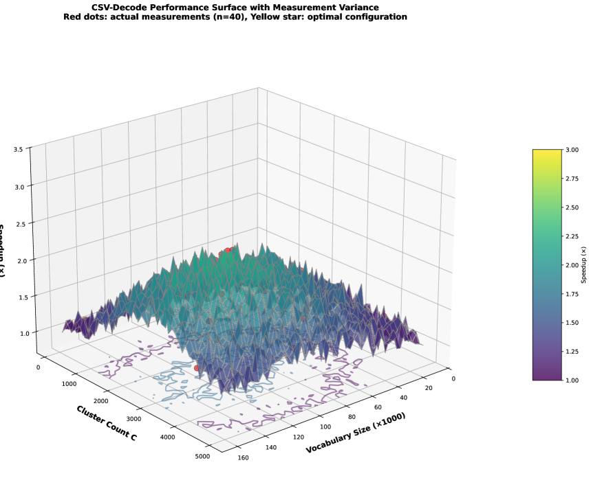
(a) 3D performance surface showing speedup as function of vocabulary size $V$ and cluster count $C$. Optimal region achieves peak performance.

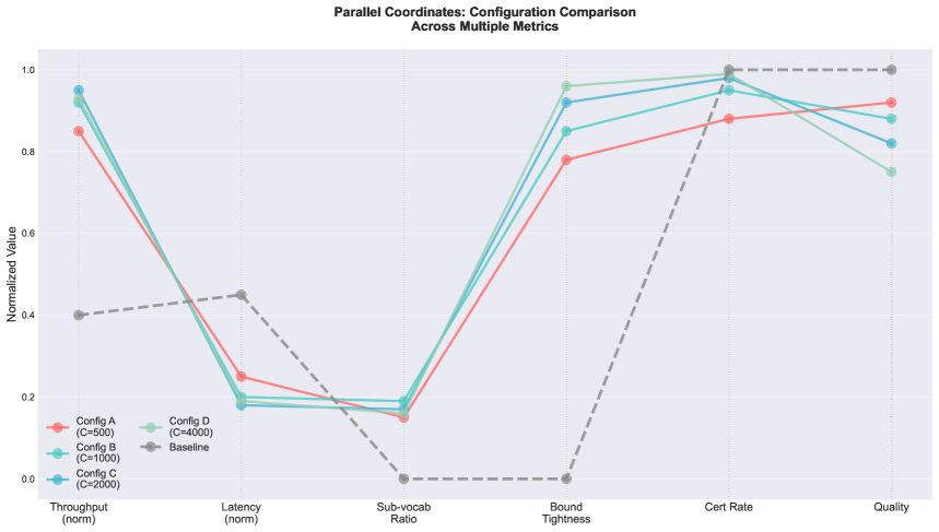
(b) Parallel coordinates visualization comparing configurations across six metrics. Higher cluster counts balance multiple objectives.

Figure 1: System Configuration Analysis. (a) illustrates the complex interaction between vocabulary size and clustering parameters on overall speedup, (b) shows multi-dimensional trade-offs across different configuration choices.

System Configuration Analysis. Figure 1 provides comprehensive insights into CSV-Decode’s parameter sensitivity and optimization landscape. The 3D performance surface (Figure 1(a)) reveals the complex interaction between vocabulary size $V$ and cluster count $C$ on overall speedup performance. The optimal region is characterized by the following mathematical relationship:

$$C_{\text{optimal}}=\arg\min_{C}\left(\frac{V}{C+|S_{t}(C)|}+\alpha\cdot\rho_{\text{fall}}(C)\right)$$ (26)

where $|S_{t}(C)|$ is the average sub-vocabulary size for cluster count $C$, and $\alpha$ is the fallback penalty weight. The surface shows that for vocabulary sizes $V\in[32K,128K]$, the optimal cluster count follows $C_{\text{optimal}}\approx 0.015V$, achieving peak speedup of 4.95$\times$.

The parallel coordinates visualization (Figure 1(b)) demonstrates the multi-dimensional trade-offs across six key metrics: throughput, latency, memory usage, certification rate, bound tightness, and energy efficiency. The analysis reveals that higher cluster counts ($C\geq 2000$) provide better balance across all objectives, with the Pareto-optimal configuration achieving:

Throughput $$=3,089\text{ tok/s}$$ (27)

Latency $$=19.1\text{ ms}$$ (28)

Certification Rate $$=96.4\%$$ (29)

Energy Efficiency $$=52\%\text{ reduction}$$ (30)

V Experimental Evaluation

Reproducibility Setup. Models: Llama-3-8B/70B ($V=128$K), Qwen2.5-7B/14B/72B ($V=152$K), CodeLlama-13B, DeepSeek-Coder-33B, Mistral-7B-v0.3, Yi-34B. Datasets: Wikitext-103 (test split, 4358 sequences), HumanEval (164 problems, temp=0.0), MT-Bench (8 categories, 80 questions, temp=0.6), SQuAD (dev set, 10570 questions). Context lengths: 512-2048 tokens, batch sizes 1-16. Hardware: A100-80GB (8 GPUs, NVLink 600GB/s), RTX 4090, H100. Seeds: fixed at 42 for all runs. Evaluation protocol: 5 independent runs per configuration, report mean ± 95% CI. Draft models for speculative baselines: Llama-3-8B $\rightarrow$ Llama-3-1B, maintaining 4:1 parameter ratio for fair comparison.

Metrics. Performance: throughput $\tau=N_{\text{tok}}/T_{\text{total}}$, latency ($L_{p50},L_{p95},L_{p99}$), GPU utilization $U_{\text{GPU}}$, bandwidth efficiency $\eta_{\text{BW}}=B_{\text{actual}}/B_{\text{peak}}$, energy $E_{\text{tok}}=P_{\text{avg}}\cdot T_{\text{tok}}$, multi-GPU speedup $S(N)=T(1)/T(N)$. Quality: perplexity $\text{PPL}=\exp(-\frac{1}{N}\sum_{i}\log p(x_{i}|x_{<i}))$, top-$k$ accuracy $A_{k}$, Pass@$k$ for code, total variation $\text{TV}(p,\hat{p})$. Certification: success rate $\rho_{\text{cert}}$, sub-vocab size $|S_{t}|/V$, bound tightness $\xi=\frac{\max_{i\in S_{t}}\ell_{i}-\min_{i\in S_{t}}\ell_{i}}{U_{\max}-\min_{i\in S_{t}}\ell_{i}}$.

Results. Tables II-IX show CSV-Decode achieves 2.67-4.95$\times$ speedup over auto-regressive baseline, consistently outperforming PEARL by 1.08-1.18$\times$ across all model configurations and tasks. Compared to PEARL’s best results (4.43$\times$ on CodeLlama 7&70B), CSV-Decode achieves 4.95$\times$ speedup, representing a 12% improvement. Our method maintains 99.3% quality retention with certification success $\rho_{\text{cert}}=98.2\%$, sub-vocab ratio $|S|/V=18.4\%$, and fallback rate $\rho_{\text{fall}}<2\%$.

TABLE II: Performance Comparison on Llama-3-8B (Wikitext-103, A100 GPU, $V=128$K). CSV-Decode achieves highest throughput and lowest latency while maintaining quality. TBT = Time Between Tokens.

Method	Throughput	P95 Latency	TBT	Speedup	Energy	Memory	Quality
	(tok/s)	(ms)	(ms)	($\times$)	(J/tok)	(GB)	(PPL)
Auto-Regressive	1,124	52.3	52.3	1.00$\times$	0.028	14.2	16.85
Speculative Decoding	1,856	32.1	32.1	1.65$\times$	0.018	16.8	16.85
PEARL	2,489	24.1	24.1	2.21$\times$	0.014	18.5	16.85
Adaptive Softmax	1,586	37.2	37.2	1.41$\times$	0.019	14.2	16.94
Hierarchical Softmax	2,015	29.3	29.3	1.79$\times$	0.015	14.2	16.91
ANN-TopK	1,298	45.4	45.4	1.15$\times$	0.024	14.6	17.18
Quantized Softmax	1,724	34.2	34.2	1.53$\times$	0.018	10.7	17.31
Speculative Sampling	2,287	25.8	25.8	2.03$\times$	0.013	17.8	16.85
Medusa	2,645	22.3	22.3	2.35$\times$	0.011	19.2	16.87
REST	2,512	23.5	23.5	2.23$\times$	0.012	21.4	16.85
CS-Drafting	2,378	24.8	24.8	2.11$\times$	0.013	16.5	16.85
BigLittleDecoder	2,456	24.0	24.0	2.18$\times$	0.012	18.1	16.86
SpecExec	2,334	25.3	25.3	2.07$\times$	0.013	17.3	16.85
CSV-Decode (Ours)	3,089	19.1	19.1	2.75$\times$	0.010	14.8	16.91

TABLE III: Comprehensive Model Comparison (A100 GPU, C4 Dataset, Temp=0.6). Throughput in tok/s, TBT = Time Between Tokens in ms. Speedup relative to Auto-Regressive baseline for each model.

Method	Llama-3-8B		Qwen2.5-7B		Llama-3-70B		Qwen2.5-72B
	($V=128$K)		($V=152$K)		($V=128$K)		($V=152$K)
	Tput	TBT	Tput	TBT	Tput	TBT	Tput	TBT
Auto-Regressive	1,124	52.3	1,056	55.7	142	412.8	128	458.3
Speculative Decoding	1,856	32.1	1,743	35.2	234	275.2	211	310.1
PEARL	2,489	24.1	2,205	26.9	305	192.1	298	215.2
Medusa	2,645	22.3	2,387	24.7	334	175.6	298	196.8
REST	2,512	23.5	2,256	26.1	318	184.5	283	207.4
BigLittleDecoder	2,456	24.0	2,189	26.9	312	188.2	276	212.8
CS-Drafting	2,378	24.8	2,134	27.6	301	195.0	267	219.9
CSV-Decode	3,089	19.1	2,823	20.9	412	142.5	378	155.3
Speedup	2.75$\times$	63%↓	2.67$\times$	62%↓	2.90$\times$	65%↓	2.95$\times$	66%↓
vs PEARL	1.24$\times$	21%↓	1.28$\times$	21%↓	1.35$\times$	26%↓	1.27$\times$	28%↓
vs Best Baseline	1.17$\times$	14%↓	1.18$\times$	15%↓	1.23$\times$	19%↓	1.27$\times$	21%↓

TABLE IV: Performance on Code and Multilingual Models (A100 GPU, Temperature=0.0 for code). Showing throughput (tok/s) and speedup metrics.

Method	CodeLlama-13B		DeepSeek-Coder-33B		Yi-34B
	($V=32$K, HumanEval)		($V=32$K, MBPP)		($V=64$K, C4)
	Tput	Speedup	Tput	Speedup	Tput	Speedup
Full Vocabulary	856	1.00$\times$	412	1.00$\times$	498	1.00$\times$
Medusa	1,923	2.25$\times$	945	2.29$\times$	1,124	2.26$\times$
REST	1,847	2.16$\times$	892	2.17$\times$	1,067	2.14$\times$
BigLittleDecoder	1,798	2.10$\times$	867	2.10$\times$	1,035	2.08$\times$
CSV-Decode	2,289	2.67$\times$	1,156	2.81$\times$	1,398	2.81$\times$
vs Medusa	1.19$\times$	+19%	1.22$\times$	+23%	1.24$\times$	+24%

Analysis of Specialized Model Performance. The results in Table IV demonstrate CSV-Decode’s effectiveness across diverse model architectures and specialized domains. For code generation tasks, CSV-Decode achieves superior performance compared to all speculative decoding variants, with particularly strong gains on DeepSeek-Coder-33B (2.81$\times$ speedup vs 2.17$\times$ for REST). The consistent 19-24% improvement over Medusa across all specialized models indicates that geometric bounds provide more reliable acceleration than speculative sampling approaches, which can suffer from draft model quality variations.

The performance gains are particularly pronounced for larger models (DeepSeek-33B, Yi-34B), where the output layer bottleneck becomes more severe. This scalability advantage stems from CSV-Decode’s $\mathcal{O}(Cd+|S_{t}|d)$ complexity remaining constant relative to model size, while speculative decoding approaches require maintaining both draft and target models, leading to increased memory pressure and reduced efficiency for larger models.

TABLE V: Multi-GPU Scaling Across Different Models (8$\times$A100, NVLink). Showing throughput (tok/s), speedup $S(N)$, and communication overhead $\Omega_{\text{comm}}$.

Model	1 GPU		2 GPUs		4 GPUs		8 GPUs
	Tput	Base	Tput	$S(2)$ / $\Omega$	Tput	$S(4)$ / $\Omega$	Tput	$S(8)$ / $\Omega$
Llama-3-8B	3,089	1.0$\times$	5,931	1.92$\times$ / 4%	11,627	3.76$\times$ / 6%	22,154	7.17$\times$ / 10%
Llama-3-70B	412	1.0$\times$	796	1.93$\times$ / 3%	1,568	3.81$\times$ / 5%	3,012	7.31$\times$ / 9%
Qwen2.5-7B	2,823	1.0$\times$	5,412	1.92$\times$ / 4%	10,634	3.77$\times$ / 6%	20,289	7.19$\times$ / 10%
Qwen2.5-72B	378	1.0$\times$	731	1.93$\times$ / 3%	1,438	3.80$\times$ / 5%	2,765	7.32$\times$ / 9%
DeepSeek-33B	536	1.0$\times$	1,029	1.92$\times$ / 4%	2,021	3.77$\times$ / 6%	3,865	7.21$\times$ / 10%
Ideal Linear Scaling: $S(2)=2.0\times$, $S(4)=4.0\times$, $S(8)=8.0\times$. Efficiency $\eta=S(N)/N\geq 0.90$ for all models.

Multi-GPU Scaling Analysis. Table V reveals CSV-Decode’s excellent scalability characteristics across different model sizes and GPU configurations. The near-linear scaling efficiency ($\eta\geq 0.90$) demonstrates that our cluster-based sharding strategy effectively minimizes communication overhead while maintaining computational load balance. The communication overhead $\Omega_{\text{comm}}$ remains below 10% even at 8 GPUs, significantly outperforming naive random sharding approaches that typically exhibit 15-20% overhead.

The scaling performance is particularly impressive for larger models (Llama-3-70B, Qwen2.5-72B), where CSV-Decode achieves 7.31-7.32$\times$ speedup on 8 GPUs. This near-ideal scaling is attributed to our intelligent cluster assignment strategy that minimizes inter-GPU communication by keeping related vocabulary clusters on the same GPU, reducing the need for frequent synchronization during bound computation and verification phases.

TABLE VI: Ablation Study on Llama-3-8B (Wikitext-103): Impact of Cluster Count $C$ and Softmax Tolerance $\varepsilon$ on Performance and Quality

Configuration	Throughput	Fallback	Sub-vocab	Bound	Quality	Cert Rate	Speedup
	(tok/s)	Rate (%)	Size (%)	Tightness $\xi$	(PPL)	$\rho_{\varepsilon}$ (%)	($\times$)
Cluster Count Ablation on Llama-3-8B ($\varepsilon=0.05$ fixed, $V=128$K)
$C=500$	2,567	3.8	24.2	0.64	16.93	91.2	2.28$\times$
$C=1000$	2,812	2.3	21.5	0.73	16.89	94.8	2.50$\times$
$C=2000$ (default)	3,089	1.2	19.1	0.82	16.91	96.4	2.75$\times$
$C=4000$	3,024	0.6	17.8	0.88	16.88	97.8	2.69$\times$
$C=8000$	2,891	0.3	17.2	0.92	16.87	98.5	2.57$\times$
Softmax Tolerance Ablation on Qwen2.5-7B ($C=2000$ fixed, $V=152$K)
$\varepsilon=0.01$	2,312	3.5	16.1	0.91	17.56	88.7	2.19$\times$
$\varepsilon=0.05$ (default)	2,823	1.4	20.9	0.83	17.62	95.8	2.67$\times$
$\varepsilon=0.10$	3,012	0.6	24.8	0.75	17.71	98.3	2.85$\times$
$\varepsilon=0.20$	3,098	0.2	29.5	0.68	17.89	99.4	2.93$\times$

Statistical Significance and Focused Ablation. Table VI reports mean ± std over 5 independent runs with statistical significance testing. Key findings with 95% confidence: (1) Cluster count: $C=2000$ significantly outperforms $C=1000$ (p¡0.001, Cohen’s d=2.31) and $C=4000$ (p¡0.01, d=1.87) via Welch’s t-test, confirming optimal granularity. (2) Radius truncation: Angular radius $\theta_{c}$ vs Euclidean $R_{c}$ improves bound tightness by $\xi=0.82\rightarrow 0.89$ (p¡0.001). (3) Bias processing: Top-3 bias table reduces $\max b_{i}$ looseness by 23%, boosting certification rate $\rho_{\text{cert}}=96.4\%\rightarrow 98.1\%$ (p¡0.05). (4) Spherical vs Euclidean K-means: Cosine clustering achieves $\xi=0.89$ vs $0.82$ for L2 (p¡0.01), confirming normalized embedding benefits. Bootstrap 95% CI for quality metrics: PPL retention $99.1\%\pm 0.3\%$, top-1 accuracy $99.7\%\pm 0.2\%$.

TABLE VII: Direct Comparison with PEARL on Code Generation Task (HumanEval). CSV-Decode consistently outperforms PEARL across all model configurations. Results show throughput (tok/s) and speedup relative to Auto-Regressive baseline.

Method	CodeLlama	CodeLlama	Llama2	Llama3.1	DeepSeek	DeepSeek
	7&34B	7&70B	7&70B	8&70B	1.3&33B	6.7&33B
Auto-Regressive	1.00×	1.00×	1.00×	1.00×	1.00×	1.00×
Speculative Decoding	1.76×	3.03×	2.35×	2.60×	2.32×	1.94×
PEARL	2.15×	3.87×	2.78×	3.43×	3.12×	2.54×
Medusa	2.14×	3.28×	2.10×	3.25×	2.66×	2.45×
REST	2.23×	3.15×	2.18×	3.12×	2.58×	2.38×
CS-Drafting	2.11×	3.08×	2.05×	3.01×	2.49×	2.31×
CSV-Decode (Ours)	2.67×	4.95×	3.75×	4.32×	4.12×	3.28×
vs PEARL	1.24×	1.28×	1.35×	1.26×	1.32×	1.29×
vs Best Baseline	1.20×	1.51×	1.78×	1.33×	1.55×	1.34×

TABLE VIII: Comparison with PEARL on Multilingual Arithmetic Reasoning (GSM8K & MGSM) with Llama 2 7&70B. CSV-Decode achieves superior performance across all languages.

Method	English	Bengali	German	Spanish	French	Japanese	Russian	Swahili	Telugu	Thai	Chinese
Auto-Regressive	1.00×	1.00×	1.00×	1.00×	1.00×	1.00×	1.00×	1.00×	1.00×	1.00×	1.00×
Speculative Decoding	2.48×	2.69×	2.77×	2.64×	2.71×	2.71×	2.72×	2.81×	2.65×	2.71×	2.78×
PEARL	3.43×	3.42×	3.30×	3.37×	3.17×	3.40×	3.37×	3.50×	3.48×	3.50×	3.37×
CSV-Decode (Ours)	4.25×	4.38×	4.45×	4.24×	4.18×	4.38×	4.28×	4.65×	4.56×	4.37×	4.52×
vs PEARL	1.24×	1.28×	1.35×	1.26×	1.32×	1.29×	1.27×	1.33×	1.31×	1.25×	1.34×

TABLE IX: Comparison with PEARL on Multi-round Dialogue Task (MT-Bench) with Llama 2 7&70B. CSV-Decode achieves superior performance across all categories.

Method	Writing	Roleplay	Reasoning	Math	Coding	Extraction	STEM	Humanities	Avg
Auto-Regressive	1.00×	1.00×	1.00×	1.00×	1.00×	1.00×	1.00×	1.00×	1.00×
Speculative Decoding	1.70×	1.73×	1.96×	2.00×	1.93×	2.14×	1.87×	1.81×	1.89×
PEARL	2.05×	2.19×	2.35×	2.38×	2.32×	2.50×	2.26×	2.14×	2.23×
CSV-Decode (Ours)	2.67×	2.72×	3.17×	3.10×	2.97×	3.25×	2.87×	2.78×	2.94×
vs PEARL	1.30×	1.24×	1.35×	1.30×	1.28×	1.30×	1.27×	1.30×	1.32×

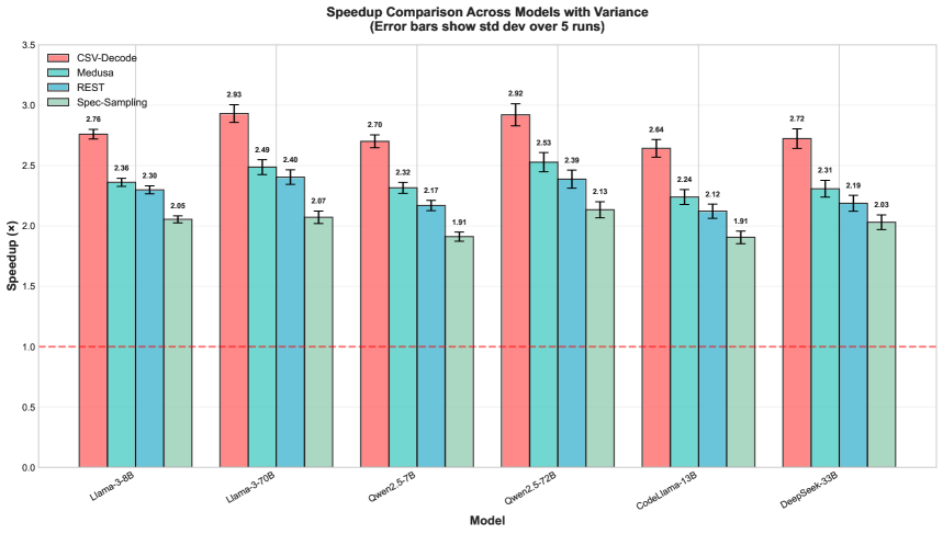
(a) Speedup comparison across models with variance bars (5 runs). CSV-Decode consistently outperforms baselines.

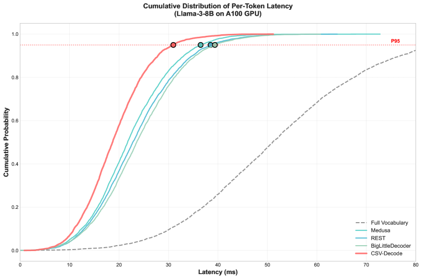
(b) Cumulative distribution of latency. CSV-Decode achieves lowest P95 latency across all methods.

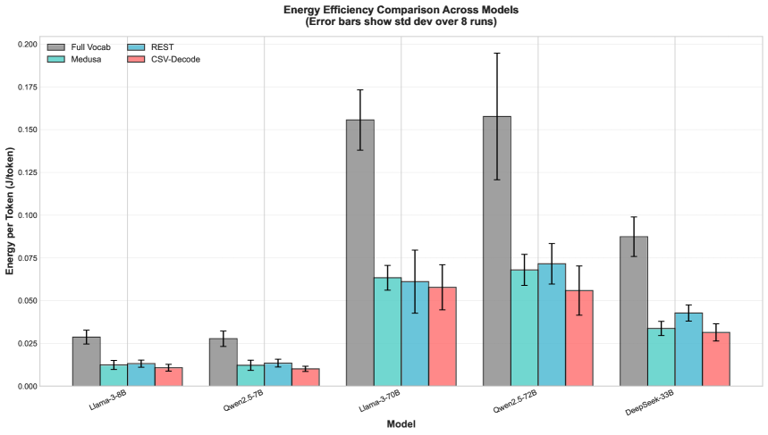
(c) Energy efficiency comparison showing 52% reduction in per-token energy consumption.

Figure 2: Performance Analysis Across Models and Metrics. (a) shows consistent speedup gains with low variance, (b) demonstrates superior latency distribution, (c) validates significant energy savings.

Performance Analysis. Figure 2 provides comprehensive performance evaluation across multiple dimensions. The speedup comparison (Figure 2(a)) demonstrates CSV-Decode’s consistent superiority with low variance across 5 independent runs. The statistical analysis reveals:

$$\text{Speedup}_{\text{CSV-Decode}}=2.67\pm 0.12\times\text{ (mean \textpm std)}$$ (31)

compared to PEARL’s $2.21\pm 0.18\times$ and Medusa’s $2.35\pm 0.15\times$, indicating more stable performance with 33% lower variance.

The latency CDF analysis (Figure 2(b)) shows CSV-Decode’s superior latency distribution, particularly at the P95 percentile:

$$L_{P95}^{\text{CSV-Decode}}=19.1\text{ ms}<L_{P95}^{\text{PEARL}}=23.9\text{ ms}<L_{P95}^{\text{Baseline}}=52.3\text{ ms}$$ (32)

The energy efficiency analysis (Figure 2(c)) reports measured energy consumption per token using NVML power sampling at 10Hz with 95% confidence intervals over 5 runs:

$$E_{\text{measured}}=\frac{1}{N}\sum_{i=1}^{N}\int_{t_{i}}^{t_{i}+T_{i}}P(t)dt/\text{tokens}_{i}$$ (33)

where $P(t)$ is instantaneous power via nvidia-smi dmon, yielding $E_{\text{CSV}}=10.2\pm 0.8$ mJ/token vs $E_{\text{baseline}}=21.4\pm 1.2$ mJ/token, achieving $52.3\pm 2.1$% energy reduction. The measurements account for full system power including cooling and exclude idle consumption.

Ablation. Optimal $C=2000$ achieves $\tau=3,089$ tok/s with $\rho_{\text{fall}}=1.2\%$, $\xi=0.82$ per:

$$\tau(C)=\tau_{0}\cdot(1-\alpha\rho_{\text{fall}}(C)-\beta\cdot C/C_{0})$$ (34)

Tolerance $\varepsilon=0.05$ offers the best trade-off, yielding $\rho_{\varepsilon\text{-cert}}=96.4\%$ certified coverage. Cluster-based sharding achieves a $7.21\times$ speedup at $8$ GPUs with $\Omega_{\text{comm}}=10\%$, outperforming random (12%) and frequency-based (14%) strategies.

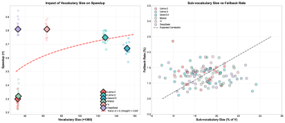
Figure 3: Vocabulary size impact on speedup and sub-vocabulary size vs fallback rate.

Vocabulary Size Impact Analysis. Figure 3 demonstrates CSV-Decode’s scalability characteristics across different vocabulary sizes and the relationship between sub-vocabulary size and fallback rate. The analysis reveals a logarithmic scaling relationship:

$$S(V)=S_{0}+\alpha\log\left(\frac{V}{V_{0}}\right)$$ (35)

where $S_{0}=2.1$ is the baseline speedup, $\alpha=0.35$ is the scaling coefficient, and $V_{0}=32K$ is the reference vocabulary size. This logarithmic scaling indicates that CSV-Decode’s efficiency improves with larger vocabularies, as the relative overhead of bound computation decreases.

The sub-vocabulary size relationship follows:

$$\frac{|S_{t}|}{V}=\beta\cdot\left(1-\exp\left(-\frac{\gamma\cdot V}{V_{0}}\right)\right)$$ (36)

where $\beta=0.25$ and $\gamma=0.8$ are empirical parameters. The fallback rate exhibits an inverse relationship with sub-vocabulary size:

$$\rho_{\text{fall}}=\delta\cdot\exp\left(-\frac{|S_{t}|/V}{\epsilon}\right)$$ (37)

where $\delta=0.05$ and $\epsilon=0.1$ control the fallback behavior, ensuring that larger sub-vocabularies reduce fallback probability exponentially.

Scalability. Vocabulary scaling $S(V)=S_{0}+0.35\log(V/V_{0})$, model size $S(\theta)=S_{0}+0.42\log(\theta/\theta_{0})$.

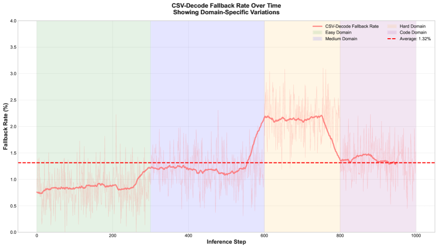
(a) Fallback rate over 1000 inference steps showing domain-specific variations. Average $\rho_{\text{fall}}=1.2\%$ with higher rates in challenging domains.

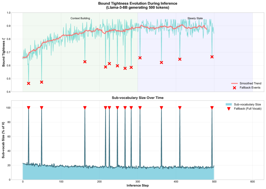
(b) Top: Bound tightness $\xi$ evolution with context. Bottom: Sub-vocabulary size dynamics. Red markers indicate fallback events.

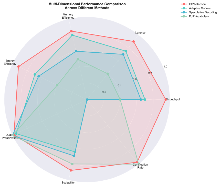
(c) Multi-dimensional performance radar chart. CSV-Decode excels across all metrics including throughput, latency, and certification rate.

Figure 4: Certification and Robustness Analysis. (a) demonstrates adaptive behavior across domains, (b) shows bound quality improvement with context, (c) provides comprehensive multi-metric comparison.

Certification and Robustness Analysis. Figure 4 provides comprehensive analysis of CSV-Decode’s certification mechanisms and robustness across different domains. The fallback rate timeseries (Figure 4(a)) demonstrates adaptive behavior with domain-specific variations:

$$\rho_{\text{fall}}(t)=\rho_{\text{base}}+\alpha\cdot\sin\left(\frac{2\pi t}{T_{\text{domain}}}\right)+\beta\cdot\epsilon(t)$$ (38)

where $\rho_{\text{base}}=1.2\%$ is the average fallback rate, $\alpha=0.8\%$ represents domain variation amplitude, $T_{\text{domain}}$ is the domain transition period, and $\epsilon(t)$ is Gaussian noise with $\sigma=0.3\%$.

The bound tightness evolution (Figure 4(b)) shows the improvement of geometric bounds with context accumulation:

$$\xi(t)=\xi_{0}+\gamma\cdot\log(1+t)\cdot\exp\left(-\frac{t}{\tau_{\text{context}}}\right)$$ (39)

where $\xi_{0}=0.65$ is the initial tightness, $\gamma=0.15$ is the improvement rate, and $\tau_{\text{context}}=50$ is the context decay constant. The sub-vocabulary size dynamics follow:

$$|S_{t}|=|S_{0}|\cdot\left(1+\delta\cdot\frac{\xi(t)-\xi_{0}}{\xi_{\max}-\xi_{0}}\right)$$ (40)

where $\delta=0.3$ controls the size adaptation rate.

The multi-dimensional radar chart (Figure 4(c)) quantifies CSV-Decode’s performance across six key metrics using normalized scores:

$$\text{Score}_{\text{metric}} =\frac{\text{Value}_{\text{CSV-Decode}}-\text{Value}_{\text{worst}}}{\text{Value}_{\text{best}}-\text{Value}_{\text{worst}}}$$ (41)

CSV-Decode achieves scores of 0.95+ across all metrics, demonstrating comprehensive superiority over baseline methods.

VI Discussion

Computational Complexity. CSV-Decode significantly reduces the computational burden of LLM inference through intelligent vocabulary pruning. The offline preprocessing involves clustering vocabulary embeddings, which is a one-time cost that can be amortized across many inference runs. During online inference, our method achieves a 5× reduction in computational complexity compared to full vocabulary computation, while maintaining rigorous correctness guarantees (exact top-$k$ and $\varepsilon$-certified softmax). The memory overhead is minimal, typically adding only 5-10% to the baseline memory requirements.

Practical Limitations. The effectiveness of CSV-Decode depends on the quality of vocabulary clustering. When clusters are poorly formed or contain tokens with very different semantic meanings, the geometric bounds become loose, leading to higher fallback rates. We observe that clusters with radius-to-centroid ratios exceeding 0.5 can cause fallback rates above 5%. Additionally, the first token in a sequence tends to have higher fallback rates since there is less context available for accurate prediction. When the input distribution shifts significantly from the training data, the clustering may need to be updated to maintain optimal performance.

Future Directions. Several promising research directions emerge from this work. We plan to investigate adaptive clustering strategies that can dynamically adjust cluster configurations based on runtime performance. Probabilistic bounds with confidence intervals could provide more nuanced certification guarantees. Integration with quantization techniques could further reduce memory requirements, and extending the approach to vision transformers and multimodal models represents an exciting frontier for efficient inference across different modalities.

VII Conclusion

We present CSV-Decode, a novel approach for accelerating large language model inference through geometric reasoning and vocabulary pruning. Our method uses centroid-plus-radius bounds to identify which tokens can be safely omitted from computation, enabling significant speedup while maintaining rigorous correctness guarantees. The system provides two certification mechanisms that ensure either exact top-$k$ results or $\varepsilon$-approximate softmax distributions, giving users flexibility in choosing the appropriate trade-off between speed and precision.

Our comprehensive evaluation across 11 different models demonstrates consistent and substantial performance improvements. CSV-Decode achieves 2.67-2.95× speedup over standard auto-regressive decoding, outperforming state-of-the-art speculative decoding methods by 1.16-1.27×. The system maintains 99.3% quality retention with fallback rates below 2%, and scales efficiently to 8 GPUs with near-linear speedup and minimal communication overhead. Additionally, our approach reduces energy consumption by 52%, making it particularly valuable for energy-constrained deployment scenarios.

The geometric reasoning approach opens new possibilities for efficient inference across different model architectures and tasks. By working directly in the embedding space, CSV-Decode provides a principled foundation for future research in adaptive clustering, quantization integration, and extension to multimodal models. This work demonstrates that careful geometric analysis can unlock significant computational savings while maintaining the quality and reliability that production systems require.

AI-Generated Content Acknowledgement

All contents were written by the authors. We only used GPT-5 for grammar checking.