New Interval Calculus with Application to Interval Differential Equations

Abstract: This paper presents a systematic study of the calculus of interval-valued functions and its application to interval differential equations. To this end, first, we introduce new interval arithmetic operations. Under new operations, the space of interval numbers becomes a strict linear space, and indeed a Hilbert space, whereas the traditional interval arithmetic yields only a semilinear space with a defective algebraic structure. Secondly, by basing derivative and integral of interval-valued functions on the proposed operations, we retain every essential property of classical calculus while seamlessly incorporating ideas from the multiplicative calculus. The resulting unified “hybrid” framework eliminates the tedious case-by-case inspection of switching points required by the gH-derivative, leading to a markedly streamlined computational procedure. Finally, we establish an existence theorem for solutions of interval differential equations within the new calculus and corroborate its validity and practicality through representative examples. In contrast to the gH-derivative approach, the number of potential solutions does not explode doubly with additional switching points, ensuring robustness in both theory and computation.

Keywords: Interval arithmetic operation; Interval-valued functions; Differentiability; Integrability; Interval differential equations

2020 MSC: 65G30; 26A06; 26E50; 34A07

1 Introduction

Interval analysis [moo, sai, JKDW01, MG17], as a mathematical approach for analyzing and handling uncertainty, captures and quantifies the uncertainty in data by representing numerical values in interval form rather than as single point values. This method has wide applications in many branches of mathematics, including inequalities [CostaTM2019, ZAYL20, ZAYL22], differential equations [SB09, MTM12, WR22, WangHZ2025], optimization [HW04, li, GYLZ22, GYT23, PengZY2025], and decision making [DaiJH2012, LiaoHC2018, YazdaniM2021, QinYJ2025]. In recent years, with the development of artificial intelligence technology, the application scope and influence of interval analysis have been further expanded, especially in engineering [HaqRSU2023, ShehadehA2024], environment [HaoY2024, ZhuJM2025], machine learning [LiWT2023, XuWH20241, MaGZ2025, SanchezL2025], economics [DragoC2022, RahmanMS2022, WangP2023, WangZZ2025], and finance [JiangMR2024, WangJJ20241, XiongT2014], where it is used to handle the inherent imprecision of real-world data that traditional real numbers cannot capture.

In 1966, Moore published the first monograph on interval analysis [moo66], which made great contributions to the early development of theory and applications of interval analysis. In this monograph, Moore presented the arithmetic operations of two intervals, i.e., for two certain intervals $\overline{a}=[a_{l},a_{r}]$ and $\overline{b}=[b_{l},b_{r}]$, then $\overline{a}\oplus\overline{b}=[a_{l}+b_{l},a_{r}+b_{r}]$ and $\overline{a}\ominus\overline{b}=[a_{l}-b_{r},a_{r}-b_{l}]$. However, if $\overline{a}\oplus\overline{b}=0$, one can not get $\overline{a}=-\overline{b}$. This leads to the space of interval numbers being a semilinear space [WR22] rather than a linear space. Moreover, besides $\overline{a}\ominus\overline{a}\neq 0$, $\overline{a}\oplus\overline{b}=\overline{c}$ does not imply that $\overline{a}=\overline{c}\ominus\overline{b}$. This indicates that there is a flaw in the operations of intervals. In order to establish a theory for interval number as real number, Hukuhara introduced a new concept of interval difference in [MH67], i.e., $\overline{a}\ominus_{H}\overline{b}=[a_{l}-b_{l},a_{r}-b_{r}]$. It is easy to see that the Hukuhara subtraction is the inverse operation of addition. However, the Hukuhara difference of two intervals does not always exist. For example, $[1,2]\ominus_{H}[3,5]=[-2,-3]$, the result does not make sense. In 1979, Markov [M79] presented a new difference of two intervals, which is consistent with the concept later called the generalized Hukuhara difference (gH-difference) by Stefanini in [Stefanini2008], i.e.,

$$\overline{a}\ominus_{gH}\overline{b}=[\min\{a_{l}-b_{l},a_{r}-b_{r}\},\max\{a_{l}-b_{l},a_{r}-b_{r}\}].$$

The gH-difference always exists, and it is the inverse operation of addition in specific situations. So it has been widely used in various papers [SB09, LS10, Chalco2013, VL15, HLO17, HVN18, CMDJ19, WR22].

On the other hand, based on the arithmetic operations of intervals, many researchers have focused on the calculus of interval-valued functions with application to interval differential equations. For example, Moore [moo] introduced the integration of interval functions, with an introduction to automatic differentiation, and used it to treat integral and differential equations. Based on the Hukuhara difference, Wu and Gong [WG2000] defined the Henstock integral of interval-valued functions, and studied the necessary and sufficient conditions of integrability and characterization of integrable interval-valued functions.

In [SB09], based on the gH-difference, Stefanini and Bede introduced two definitions for the derivative of an interval-valued function and their properties. Moreover, local existence and uniqueness of two solutions was obtained together with characterizations of the solutions of an interval differential equation by ODE systems. Later in [MTM12], an interval initial value problem with a second type Hukuhara derivative was considered. The existence of solutions, continuous dependence of the solution on initial value, and the compactness of solutions set were shown. In [Chalco2013], conditions, examples and counterexamples for limit, continuity, integrability, and differentiability for interval-valued functions were given by using the generalized Hukuhara differentiability. In [WR22], some sufficient conditions are provided in order to deduce the existence of solutions without switching points, and also for mixed solutions with a unique switching point, while stopping time problem of the first order multidimensional interval-valued dynamic system was discussed in [WangHZ2025]. These advancements have not only enriched the theoretical foundations but also broadened the scope of applications, particularly in fuzzy systems and stochastic analysis. However, due to the existence of two types of derivative, it is necessary to consider the problem of switching points during the differentiation process [Qiu23]. Furthermore, when solving differential equations, as the domain expands, the number of solutions to the equation may increase doubly.

After observing the shortcomings of previous literatures in interval analysis, particularly the algebraic deficiencies of traditional interval arithmetic operations, this work emerges to address several critical limitations. The conventional approach renders the space of interval numbers $\mathbb{R}_{\mathcal{I}}$ merely a semilinear space, creating substantial obstacles in developing a consistent calculus for interval-valued functions. These structural weaknesses manifest most prominently in differentiation and integration theories, where existing definitions lead to operational inconsistencies and computational complexities. This work aims to contribute to this growing body of knowledge by addressing key challenges and exploring new directions in the calculus of interval-valued functions.

Motivated by these challenges, we introduce novel arithmetic operations that restore complete linearity to $\mathbb{R}_{\mathcal{I}}$, transforming it into a proper Hilbert space equipped with a well-defined inner product “$\diamond$” and norm $\|\cdot\|$. This enhanced structure enables us to propose:

• A new derivative concept unifying classical and multiplicative approaches;

• An integral definition overcoming previous computational limitations;

• A rigorous framework for interval differential equations.

The proposed calculus demonstrates superior computational efficiency compared to existing methods, while maintaining intuitive interpretability for applications ranging from uncertainty quantification to growth process modeling. Our results not only resolve long-standing theoretical inconsistencies, but also provide practical tools for working with interval-valued functions in scientific computing and engineering applications.

The rest of the paper are organized as follows. In Section 2, we present new interval arithmetic operations, which lead to the space of all interval numbers being a linear space. Further, by introducing new distance, norm, and inner product formulas, we prove that the space of all interval numbers is a Hilbert space. Section 3 introduces the interval-valued function and its continuity. Under the new norm, the space of continuous interval-valued functions is a Banach space. Section 4 mainly introduces the new concept of the derivative of interval-valued functions and its related properties. The new derivative is a combination of the traditional derivative and the multiplicative derivative, which simplifies the differentiation of interval-valued functions and eliminates the need to consider the switching points. Compared to the gH-derivative, our derivative has advantages in computation. In Section 5, we consider the Riemann-type integral of interval-valued functions and present many related properties, including linearity, monotonicity, subinterval integrability, and additivity. At the same time, the fundamental theorem of calculus, integration by parts formula, monotone convergence theorem, and dominated convergence theorem are also proved. In Section 6, by using the well-known Schauder’s fixed point theorem, we present an existence theorem for the solutions of interval differential equations and demonstrate the effectiveness and practicality of our method through several specific examples.

2 The Space $\mathbb{R}_{\mathcal{I}}$

Let $\mathbb{R}$ be the set of real numbers, and $a_{l},a_{r}\in\mathbb{R}$ with $a_{l}<a_{r}$, the closed interval $\overline{a}=[a_{l},a_{r}]$ is called an interval number. Denote by $\mathbb{R}_{\mathcal{I}}$ the set of all interval numbers, i.e.,

$$\mathbb{R}_{\mathcal{I}}=\{\overline{a}~|~\overline{a}=[a_{l},a_{r}],~a_{l}<a_{r}\}.$$

In this paper, real numbers are NOT considered as (degenerate) interval numbers.

For any interval number $\overline{a}=[a_{l},a_{r}]\in\mathbb{R}_{\mathcal{I}}$, let

$$a_{c}=\frac{a_{l}+a_{r}}{2},\qquad a_{w}=\frac{a_{r}-a_{l}}{2}.$$ (2.1)

Then $a_{c}$ $(\in\mathbb{R})$ is called the center of $\overline{a}$ and $a_{w}$ $(>0)$ is called the radius of $\overline{a}$. In fact, for any interval number, its center and radius are unique. In this sense, we can rewrite the interval number $\overline{a}=[a_{l},a_{r}]$ by

$$\overline{a}\triangleq\langle a_{c};a_{w}\rangle.$$

This notation is also shown in many papers, such as [BS14, Stefanini19, Stefanini192].

2.1 Orderings

This subsection is devoted to some common used orderings in $\mathbb{R}_{\mathcal{I}}$.

Definition 2.1.

([BS14]) For any $\overline{a},\overline{b}\in\mathbb{R}_{\mathcal{I}},$ $\overline{a}=\langle a_{c};a_{w}\rangle$, $\overline{b}=\langle b_{c};b_{w}\rangle,$ we say that

1. $\overline{a}=\overline{b}$ if $a_{c}=b_{c}$ and $a_{w}=b_{w}$.

2. $\overline{a}<\overline{b}$ if $a_{c}<b_{c}$ or $a_{c}=b_{c}$ and $a_{w}<b_{w}$.

3. $\overline{a}\leq\overline{b}$ if $\overline{a}<\overline{b}$ or $\overline{a}=\overline{b}$.

Let $\overline{a},~\overline{b}\in\mathbb{R}_{\mathcal{I}}$, $\overline{a}=\langle a_{c};a_{w}\rangle$, $\overline{b}=\langle b_{c};b_{w}\rangle,$ the function $\phi:\mathbb{R}_{\mathcal{I}}\times\mathbb{R}_{\mathcal{I}}\to\mathbb{R}$ is given by

$$\phi(\overline{a},\overline{b})=(a_{c}-b_{c})+\left(1-{\mathrm{sgn}(|a_{c}-b_{c}|)}\right)\left(\frac{a_{w}}{b_{w}}-1\right),$$ (2.2)

where $\mathrm{sgn}(.)$ is the signum function.

Lemma 2.2.

Assume that $\overline{a},~\overline{b}\in\mathbb{R}_{\mathcal{I}}$, then $\overline{a}\leq\overline{b}$ if and only if $\phi(\overline{a},\overline{b})\leq 0.$

Proof.

(Sufficiency) Since $\phi(\overline{a},\overline{b})\leq 0,$ if $a_{c}\neq b_{c}$, then

$$\phi(\overline{a},\overline{b})=a_{c}-b_{c}\leq 0,$$

hence, $a_{c}<b_{c},$ which implies $\overline{a}<\overline{b}$; if $a_{c}=b_{c}$, then

$$\phi(\overline{a},\overline{b})=\frac{a_{w}}{b_{w}}-1\leq 0,$$

i.e., $a_{w}\leq b_{w},$ which implies $\overline{a}\leq\overline{b}$.

(Necessity) If $\overline{a}=\overline{b}$, then $a_{c}=b_{c}$ and $a_{w}=b_{w}$. Therefore

$$\phi(\overline{a},\overline{b})=0.$$

If $\overline{a}<\overline{b}$, then $a_{c}<b_{c}$ or $a_{c}=b_{c}$ and $a_{w}<b_{w}$. When $a_{c}<b_{c}$, one has

$$\phi(\overline{a},\overline{b})=a_{c}-b_{c}<0.$$

When $a_{c}=b_{c}$ and $a_{w}<b_{w}$, one has

$$\phi(\overline{a},\overline{b})=\frac{a_{w}}{b_{w}}-1<0.$$

The proof is therefore complete. ∎

Example 2.3.

Consider the interval numbers $\overline{a}=[0,3],~\overline{b}=[1,2],~\overline{c}=[3,4].$ Then we have

$$\phi(a,b)=2>0,\qquad\phi(a,c)=-2<0.$$

Thus, $b<a<c$.

Definition 2.4.

([BS14]) For any $\overline{a},\overline{b}\in\mathbb{R}_{\mathcal{I}}$, $\overline{a}=\langle a_{c};a_{w}\rangle$, $\overline{b}=\langle b_{c};b_{w}\rangle,$ we define

• $\overline{a}\preccurlyeq\overline{b}$ if $a_{c}\leq b_{c}$ and $a_{w}\leq b_{w}$.

• $\overline{a}\prec\overline{b}$ if $\overline{a}\preccurlyeq\overline{b}$ but $\overline{a}\neq\overline{b}$.

By Definitions 2.1 and 2.4, we have

Lemma 2.5.

If $\overline{a}\preccurlyeq\overline{b}$ then $\overline{a}\leq\overline{b}$, but not vice versa.

Definition 2.6.

([ZDF19]) For any $\overline{a},\overline{b}\in\mathbb{R}_{\mathcal{I}}$, $\overline{a}=\langle a_{c};a_{w}\rangle$, $\overline{b}=\langle b_{c};b_{w}\rangle,$ we define

• $\overline{a}\subseteq\overline{b}$ if $b_{l}\leq a_{l}<a_{r}\leq b_{r}$ .

• $\overline{a}\subset\overline{b}$ if $\overline{a}\subseteq\overline{b}$ but $\overline{a}\neq\overline{b}$.

Remark 2.7.

From Definitions 2.1, 2.4, and 2.6, it is easy to see that $``\leq"$ is a total ordering, while $``\subseteq"$ and $``\preccurlyeq"$ are partial orderings.

By Definitions 2.1, 2.4, 2.6, and (2.1), one has

Proposition 2.8.

The following statements are equivalent:

1. $\overline{a}=\overline{b}$;

2. $a_{c}=b_{c}$ and $a_{w}=b_{w}$;

3. $a_{l}=b_{l}$ and $a_{r}=b_{r}$;

4. $\overline{a}\leq\overline{b}$ and $\overline{b}\leq\overline{a}$.

5. $\overline{a}\subseteq\overline{b}$ and $\overline{b}\subseteq\overline{a}$.

6. $\overline{a}\preccurlyeq\overline{b}$ and $\overline{b}\preccurlyeq\overline{a}$.

2.2 Arithmetic Operations

In this subsection, we introduce new arithmetic operations of interval numbers, and make a comparison with the classical interval operations.

2.2.1 Addition

Definition 2.9.

For any $\overline{a},\overline{b}\in\mathbb{R}_{\mathcal{I}}$, we define

$$\overline{a}+\overline{b}=\langle a_{c}+b_{c};a_{w}b_{w}\rangle.$$ (2.3)

Lemma 2.10.

For any $\overline{a},\overline{b}\in\mathbb{R}_{\mathcal{I}}$, there exists a unique $\overline{c}=[c_{l},c_{r}]$ in $\mathbb{R}_{\mathcal{I}}$ such that $\overline{c}=\overline{a}+\overline{b}$, and

$$c_{l}=\frac{2(a_{l}+a_{r}+b_{l}+b_{r})-(a_{r}-a_{l})(b_{r}-b_{l})}{4},$$

$$c_{r}=\frac{2(a_{l}+a_{r}+b_{l}+b_{r})+(a_{r}-a_{l})(b_{r}-b_{l})}{4}.$$

Proof.

By Definition 2.9, we have

$$\overline{a}+\overline{b}$$

$$= \langle a_{c}+b_{c};a_{w}b_{w}\rangle$$

$$= [a_{c}+b_{c}-a_{w}b_{w},a_{c}+b_{c}+a_{w}b_{w}]$$

$$= \left[\frac{a_{l}+a_{r}}{2}+\frac{b_{l}+b_{r}}{2}-\frac{a_{r}-a_{l}}{2}\frac{b_{r}-b_{l}}{2},\frac{a_{l}+a_{r}}{2}+\frac{b_{l}+b_{r}}{2}+\frac{a_{r}-a_{l}}{2}\frac{b_{r}-b_{l}}{2}\right]$$

$$= \left[\frac{2(a_{l}+a_{r}+b_{l}+b_{r})-(a_{r}-a_{l})(b_{r}-b_{l})}{4},\frac{2(a_{l}+a_{r}+b_{l}+b_{r})+(a_{r}-a_{l})(b_{r}-b_{l})}{4}\right].$$

Let

$$c_{l}=\frac{2(a_{l}+a_{r}+b_{l}+b_{r})-(a_{r}-a_{l})(b_{r}-b_{l})}{4},$$

$$c_{r}=\frac{2(a_{l}+a_{r}+b_{l}+b_{r})+(a_{r}-a_{l})(b_{r}-b_{l})}{4},$$

then we have $\overline{c}=\overline{a}+\overline{b}$. ∎

Proposition 2.11.

For any $\overline{a},~\overline{b},~\overline{c},~\overline{d}\in\mathbb{R}_{\mathcal{I}},$ one has

1. $\overline{a}+\overline{b}=\overline{b}+\overline{a};$

2. $\overline{a}+(\overline{b}+\overline{c})=(\overline{a}+\overline{b})+\overline{c};$

3. there exists a unique zero element $\overline{0}=\langle 0;1\rangle=[-1,1]$ such that $\overline{a}+\overline{0}=\overline{a};$

4. there exists a unique $\overline{e}\in\mathbb{R}_{\mathcal{I}}$ such that $\overline{a}+\overline{e}=\overline{0},$ here $\overline{e}$ is called the negative element of $\overline{a}$ and denoted by $\overline{e}=-\overline{a}$;

5. $\overline{a}+\overline{c}\leq\overline{b}+\overline{c}$ if and only if $\overline{a}\leq\overline{b}$;

6. $\overline{a}\leq\overline{b}$ and $\overline{c}\leq\overline{d}$ implies $\overline{a}+\overline{c}\leq\overline{b}+\overline{d}$.

Proof.

(1) $\overline{a}+\overline{b}=\langle a_{c}+b_{c};a_{w}b_{w}\rangle=\langle b_{c}+a_{c};b_{w}a_{w}\rangle=\overline{b}+\overline{a}$.

(2) $\overline{a}+(\overline{b}+\overline{c})=\langle a_{c};a_{w}\rangle+\langle b_{c}+c_{c};b_{w}c_{w}\rangle=\langle a_{c}+b_{c}+c_{c};a_{w}b_{w}c_{w}\rangle.$

$(\overline{a}+\overline{b})+\overline{c}=\langle a_{c}+b_{c};a_{w}b_{w}\rangle+\langle c_{c};c_{w}\rangle=\langle a_{c}+b_{c}+c_{c};a_{w}b_{w}c_{w}\rangle.$

Hence, $\overline{a}+(\overline{b}+\overline{c})=(\overline{a}+\overline{b})+\overline{c}.$

(3) Let $\overline{0}=\langle 0_{c};0_{w}\rangle,$ then we have

$$\overline{a}+\overline{0}=\langle a_{c}+0_{c};a_{w}0_{w}\rangle=\langle a_{c};a_{w}\rangle=\overline{a}.$$

This implies $0_{c}=0$ and $0_{w}=1$, i.e., $\overline{0}=\langle 0;1\rangle=[-1,1].$ Hence, $\overline{0}=[-1,1]$ is the zero element in $\mathbb{R}_{\mathcal{I}}$, and the uniqueness is obvious.

(4) Let $\overline{e}=\langle e_{c};e_{w}\rangle$ such that $\overline{a}+\overline{e}=\overline{0}.$ Then, according to Definition 2.9, we have

$$a_{c}+e_{c}=0,~~a_{w}e_{w}=1.$$

Thus,

$$\overline{e}=-\overline{a}=\left\langle-a_{c};\frac{1}{a_{w}}\right\rangle.$$

Hence, for any number $\overline{a}$, the negative element $-\overline{a}=\langle-a_{c};\frac{1}{a_{w}}\rangle$, and the uniqueness is obvious.

(5) Since

$$\phi(\overline{a}+\overline{c},\overline{b}+\overline{c})$$

$$= ((a_{c}+c_{c})-(b_{c}+c_{c}))+\left(1-{\mathrm{sgn}(|(a_{c}+c_{c})-(b_{c}+c_{c})|)}\right)\left(\frac{a_{w}c_{w}}{b_{w}c_{w}}-1\right),$$

$$= (a_{c}-b_{c}))+\left(1-{\mathrm{sgn}(|a_{c}-b_{c}|)}\right)\left(\frac{a_{w}}{b_{w}}-1\right),$$

$$= \phi(\overline{a},\overline{b}),$$

Thus, by Theorem 2.2, $\overline{a}+\overline{c}\leq\overline{b}+\overline{c}$ if and only if $\overline{a}\leq\overline{b}$.

(6) Since $\overline{a}\leq\overline{b}$ and $\overline{c}\leq\overline{d}$, according to Definition 2.1, we have

$$a_{c}<b_{c},\text{ or }a_{c}=b_{c},~0<a_{w}\leq b_{w},$$

and

$$c_{c}<d_{c},\text{ or }c_{c}=d_{c},~0<c_{w}\leq d_{w}.$$

It is easy to obtain

$$\left\{\begin{array}[]{ll}a_{c}+c_{c}=b_{c}+d_{c},~a_{w}c_{w}\leq b_{w}d_{w},~\text{or}\\ a_{c}+c_{c}<b_{c}+d_{c},\end{array}\right.$$

that is,

$$\overline{a}+\overline{c}\leq\overline{b}+\overline{d}.$$

Therefore, we complete the proof. ∎

Recall that, in [moo66] and the references therein, the sum is defined as

$$\overline{a}\oplus\overline{b}=[a_{l}+b_{l},a_{r}+b_{r}]=\langle a_{c}+b_{c};a_{w}+b_{w}\rangle.$$ (2.4)

From (2.3) and (2.4), it is easy to see that the sums $\overline{a}+\overline{b}$ and $\overline{a}\oplus\overline{b}$ have the same center, but their radiuses depend on the radiuses of $\overline{a}$ and $\overline{b}$. Moreover, we have

Proposition 2.12.

For any $\overline{a},\overline{b}\in\mathbb{R}_{\mathcal{I}}$, Let $\overline{c}=\overline{a}+\overline{b}$, and $\overline{d}=\overline{a}\oplus\overline{b}$.

1. If $\frac{1}{a_{w}}+\frac{1}{b_{w}}=1$, then $\overline{c}=\overline{d};$

2. If $\frac{1}{a_{w}}+\frac{1}{b_{w}}<1$, then $\overline{d}\subset\overline{c};$

3. If $\frac{1}{a_{w}}+\frac{1}{b_{w}}>1$, then $\overline{c}\subset\overline{d}.$

Proof.

(1) If $\frac{1}{a_{w}}+\frac{1}{b_{w}}=1$, then we have $a_{w}+b_{w}=a_{w}b_{w}$, which implies

$$\langle a_{c}+b_{c};a_{w}b_{w}\rangle=\langle a_{c}+b_{c};a_{w}+b_{w}\rangle,$$

that is,

$$\overline{c}=\overline{a}+\overline{b}=\overline{a}\oplus\overline{b}=\overline{d}.$$

The proofs of (2) and (3) are similar to that of (1). ∎

Example 2.13.

Considering that $\overline{a}=[-5,-1]$, $\overline{b}_{1}=[1,3]$, $\overline{b}_{2}=[1,5]$, $\overline{b}_{3}=[1,7]$, then

$$\overline{a}+\overline{b}_{1}=\left[-3,1\right],\quad\overline{a}+\overline{b}_{2}=\left[-4,4\right],\quad\overline{a}+\overline{b}_{3}=\left[-5,7\right],$$

and

$$\overline{a}\oplus\overline{b}_{1}=\left[-4,2\right],\quad\overline{a}\oplus\overline{b}_{2}=\left[-4,4\right],\quad\overline{a}\oplus\overline{b}_{3}=\left[-4,6\right].$$

2.2.2 Scalar Multiplication

Definition 2.14.

For any $\overline{a}\in\mathbb{R}_{\mathcal{I}}$ and $k\in\mathbb{R}$, we define

$$k\cdot\overline{a}=k\overline{a}=\langle ka_{c};a_{w}^{k}\rangle.$$ (2.5)

Lemma 2.15.

For any $\overline{a}\in\mathbb{R}_{\mathcal{I}}$ and $k\in\mathbb{R}$, there exists a unique $\overline{c}=[c_{l},c_{r}]$ in $\mathbb{R}_{\mathcal{I}}$ such that $\overline{c}=k\overline{a}$, and

$$c_{l}=ka_{c}-a_{w}^{k},\qquad c_{r}=ka_{c}+a_{w}^{k}.$$

Proof.

This conclusion can be directly gotten from Definition 2.14. ∎

Proposition 2.16.

For any $\overline{a},\overline{b}\in\mathbb{R}_{\mathcal{I}}$ and $k,l\in\mathbb{R}$, then

1. $1\overline{a}=\overline{a};$

2. $k(\overline{a}+\overline{b})=k\overline{a}+k\overline{b};$

3. $(k+l)\overline{a}=k\overline{a}+l\overline{a};$

4. $(kl)\overline{a}=k(l\overline{a}).$

5. $\overline{a}\leq\overline{b}$ implies $k\overline{a}\leq k\overline{b}$ if $k\geq 0$, or $k\overline{a}\geq k\overline{b}$ if $k<0$.

Proof.

(1) $1\overline{a}=\langle 1a_{c};a_{w}^{1}\rangle=\langle a_{c};a_{w}\rangle=\overline{a}$.

(2) Since

$$k(\overline{a}+\overline{b})=\langle k(a_{c}+b_{c});(a_{w}b_{w})^{k}\rangle$$

and

$$k\overline{a}+k\overline{b}=\langle ka_{c};a_{w}^{k}\rangle+\langle kb_{c};b_{w}^{k}\rangle=\langle ka_{c}+kb_{c};a_{w}^{k}b_{w}^{k}\rangle,$$

then

$$k(\overline{a}+\overline{b})=k\overline{a}+k\overline{b}.$$

(3) Since

$$(k+l)\overline{a}=\langle(k+l)a_{c};a_{w}^{k+l}\rangle,$$

and

$$k\overline{a}+l\overline{a}=\langle ka_{c};a_{w}^{k}\rangle+\langle la_{c};a_{w}^{l}\rangle=\langle(k+l)a_{c};a_{w}^{k+l}\rangle,$$

then

$$(k+l)\overline{a}=k\overline{a}+l\overline{a}.$$

(4) Since

$$(kl)\overline{a}=\langle kla_{c};a_{w}^{kl}\rangle,$$

and

$$k(la)=k\langle la_{c};a_{w}^{l}\rangle=\langle kla_{c};a_{w}^{kl}\rangle,$$

then

$$(kl)\overline{a}=k(l\overline{a}).$$

(5) Since $\overline{a}\leq\overline{b}$, according to Definition 2.1, we have

$$\left\{\begin{array}[]{ll}a_{c}=b_{c},~a_{w}\leq b_{w},~\text{or}\\ a_{c}<b_{c}.\end{array}\right.$$

If $k\geq 0$, then we have

$$\left\{\begin{array}[]{ll}ka_{c}=kb_{c},~a_{w}^{k}\leq b_{w}^{k},~\text{or}\\ ka_{c}<kb_{c},\end{array}\right.$$

which implies $k\overline{a}\leq k\overline{b}$.

If $k<0$, then we have

$$\left\{\begin{array}[]{ll}ka_{c}=kb_{c},~a_{w}^{k}\geq b_{w}^{k},~\text{or}\\ ka_{c}>kb_{c},\end{array}\right.$$

which implies $k\overline{a}\geq k\overline{b}$.

Thus, we complete the proof. ∎

Remark 2.17.

By Proposition 2.11 (4) and Definition 2.14, when $k=-1$, we have $-\overline{a}=(-1)\overline{a}$. In fact, for any interval number $\overline{a}=\langle a_{c};a_{w}\rangle$, one has

$$-\overline{a}=\langle-a_{c};a_{w}^{-1}\rangle=-1\langle a_{c};a_{w}\rangle=-1\overline{a}.$$

Proposition 2.18.

Let $\overline{a}_{i}=\left\langle(a_{i})_{c};(a_{i})_{w}\right\rangle\in\mathbb{R}_{\mathcal{I}}$, $k_{i}\in\mathbb{R}$, $i=1,2,...,n$. Then

$$\sum_{i=1}^{n}k_{i}\overline{a}_{i}=\left\langle\sum_{i=1}^{n}k_{i}(a_{i})_{c};\prod_{i=1}^{n}(a_{i})_{w}^{k_{i}}\right\rangle.$$

Recall that, in [moo66] and the references therein, the scalar multiplication is defined as

$$k\odot\overline{a}=\begin{cases}[ka_{l},ka_{r}]=\langle ka_{c};ka_{w}\rangle,&\text{ if }k\geq 0,\\ [ka_{r},ka_{l}]=\langle ka_{c};-ka_{w}\rangle,&\text{ if }k<0.\end{cases}$$ (2.6)

According to (2.5) and (2.6), the scalar multiplication $\overline{c}$ and $\overline{d}$ have the same center, but their radiuses depend on the radius of $\overline{a}$ and $k$. Moreover, one has

Proposition 2.19.

For any $\overline{a}\in\mathbb{R}_{\mathcal{I}}$, $k\in\mathbb{R}$, Let $\overline{c}=k\overline{a}$, and $\overline{d}=k\odot\overline{a}$.

• If $|k|a_{w}=a_{w}^{k}$, then $\overline{c}=\overline{d};$

• If $|k|a_{w}<a_{w}^{k}$, then $\overline{d}\subset\overline{c};$

• If $|k|a_{w}>a_{w}^{k}$, then $\overline{c}\subset\overline{d}.$

Proof.

(1) If $|k|{a_{w}}={a_{w}}^{k}$, then we have

$$\langle ka_{c};a_{w}^{k}\rangle=\langle ka_{c};|k|a_{w}\rangle=\begin{cases}\langle ka_{c};ka_{w}\rangle,&\text{ if }k\geq 0,\\ \langle ka_{c};-ka_{w}\rangle,&\text{ if }k<0,\\ \end{cases}$$

that is,

$$\overline{c}=k\overline{a}=k\odot\overline{a}=\overline{d}.$$

The proofs of (2) and (3) are similar to that of (1). ∎

Example 2.20.

Considering that $\overline{a}_{1}=[-2,-1]$, $\overline{a}_{2}=[1,5]$, $\overline{a}_{3}=[1,9]$, then

$$k\overline{a}_{1}=\begin{cases}[-\frac{1}{2},\frac{7}{2}],&\text{ if }k=-1,\\ [-1,1],&\text{ if }k=0,\\ [-\frac{3}{4}-\frac{\sqrt{2}}{2},-\frac{3}{4}+\frac{\sqrt{2}}{2}],&\text{ if }k=\frac{1}{2},\\ [-2,-1],&\text{ if }k=1,\\ [-\frac{13}{4},-\frac{11}{4}],&\text{ if }k=2,\\ \end{cases}\qquad\text{~and~}k\odot\overline{a}_{1}=\begin{cases}[1,2],&\text{ if }k=-1,\\ 0,&\text{ if }k=0,\\ [-1,-\frac{1}{2}],&\text{ if }k=\frac{1}{2},\\ [-2,-1],&\text{ if }k=1,\\ [-4,-2],&\text{ if }k=2,\\ \end{cases}$$

$$k\overline{a}_{2}=\begin{cases}[-\frac{7}{2},-\frac{5}{2}],&\text{ if }k=-1,\\ [-1,1],&\text{ if }k=0,\\ [1,5],&\text{ if }k=1,\\ [\frac{9}{2}-2\sqrt{2},\frac{9}{2}+2\sqrt{2}],&\text{ if }k=1.5,\\ [2,10],&\text{ if }k=2,\\ [1,17],&\text{ if }k=3,\\ \end{cases}\qquad\text{~and~}k\odot\overline{a}_{2}=\begin{cases}[-5,-1],&\text{ if }k=-1,\\ 0,&\text{ if }k=0,\\ [1,5],&\text{ if }k=1,\\ [\frac{3}{2},\frac{15}{2}],&\text{ if }k=1.5,\\ [2,10],&\text{ if }k=2,\\ [3,15],&\text{ if }k=3,\\ \end{cases}$$

$$k\overline{a}_{3}=\begin{cases}[-3,-2],&\text{ if }k=-\frac{1}{2},\\ [-1,1],&\text{ if }k=0,\\ [\frac{1}{2},\frac{9}{2}],&\text{ if }k=\frac{1}{2},\\ [\frac{15}{4}-2\sqrt{2},\frac{15}{4}+2\sqrt{2}],&\text{ if }k=\frac{3}{4},\\ [1,9],&\text{ if }k=1,\\ [-6,26],&\text{ if }k=2,\\ \end{cases}\qquad\text{~and~}k\odot\overline{a}_{3}=\begin{cases}[-\frac{9}{2},-\frac{1}{2}],&\text{ if }k=-\frac{1}{2},\\ 0,&\text{ if }k=0,\\ [\frac{1}{2},\frac{9}{2}],&\text{ if }k=\frac{1}{2},\\ [\frac{3}{4},\frac{27}{4}],&\text{ if }k=\frac{3}{4},\\ [1,9],&\text{ if }k=1,\\ [2,18],&\text{ if }k=2.\\ \end{cases}$$

2.2.3 Subtraction

Definition 2.21.

For any $\overline{a},~\overline{b}\in\mathbb{R}_{\mathcal{I}}$, we define

$$\overline{a}-\overline{b}=\left\langle a_{c}-b_{c};\frac{a_{w}}{b_{w}}\right\rangle=\left[a_{c}-b_{c}-\frac{a_{w}}{b_{w}},a_{c}-b_{c}+\frac{a_{w}}{b_{w}}\right].$$ (2.7)

It follows from Definition 2.21 that for any $\overline{a}\in\mathbb{R}_{\mathcal{I}}$,

$$\overline{a}-\overline{a}=\left\langle 0;1\right\rangle=\overline{0}.$$

By Definition 2.21 and Remark 2.17, the following statement holds.

Lemma 2.22.

For any $\overline{a},~\overline{b}\in\mathbb{R}_{\mathcal{I}}$, we have

$$\overline{a}-\overline{b}=\overline{a}+(-\overline{b})=\overline{a}+(-1\overline{b}).$$

Theorem 2.23.

Let $\overline{a},~\overline{b},~\overline{c}\in\mathbb{R}_{\mathcal{I}}$. If $\overline{a}+\overline{b}=\overline{c}$, then $\overline{a}=\overline{c}-\overline{b}$.

Proof.

Since $\overline{a}+\overline{b}=\overline{c}$, we have

$$c_{c}=a_{c}+b_{c},\qquad c_{w}=a_{w}b_{w}.$$

Thus

$$a_{c}=c_{c}-b_{c},\qquad a_{w}=\frac{c_{w}}{b_{w}}.$$

That is,

$$\overline{a}=\overline{c}-\overline{b}.$$

This ends the proof. ∎

Remark 2.24.

Theorem 2.23 implies that the subtraction defined in Definition 2.21 is the inverse arithmetic of the addition given Definition 2.9.

Proposition 2.25.

For any $\overline{a},~\overline{b},~\overline{c}\in\mathbb{R}_{\mathcal{I}}$, one has

• $\overline{a}+(\overline{b}-\overline{c})=\overline{a}+\overline{b}-\overline{c}=\overline{a}-\overline{c}+\overline{b}=\overline{a}-(\overline{c}-\overline{b})$;

• $\overline{a}-(\overline{b}+\overline{c})=\overline{a}-\overline{b}-\overline{c};$

• $k(\overline{a}-\overline{b})=k\overline{a}-k\overline{b},$ for any $k\in\mathbb{R}$;

• $(k-l)\overline{a}=k\overline{a}-l\overline{a},$ for any $k,l\in\mathbb{R}$.

Proof.

(1) For any $\overline{a},~\overline{b},~\overline{c}\in\mathbb{R}_{\mathcal{I}}$, one has

$$\overline{a}+(\overline{b}-\overline{c})=\left\langle a_{c};{a_{w}}\right\rangle+\left\langle b_{c}-c_{c};\frac{b_{w}}{c_{w}}\right\rangle=\left\langle a_{c}+b_{c}-c_{c};\frac{a_{w}b_{w}}{c_{w}}\right\rangle,$$

$$\overline{a}+\overline{b}-\overline{c}=\left\langle a_{c}+b_{c};{a_{w}}{b_{w}}\right\rangle-\left\langle c_{c};{c_{w}}\right\rangle=\left\langle a_{c}+b_{c}-c_{c};\frac{a_{w}b_{w}}{c_{w}}\right\rangle,$$

$$\overline{a}-\overline{c}+\overline{b}=\left\langle a_{c}-c_{c};\frac{a_{w}}{c_{w}}\right\rangle+\left\langle b_{c};{b_{w}}\right\rangle=\left\langle a_{c}+b_{c}-c_{c};\frac{a_{w}b_{w}}{c_{w}}\right\rangle,$$

$$\overline{a}-(\overline{c}-\overline{b})=\left\langle a_{c};{a_{w}}\right\rangle-\left\langle c_{c}-b_{c};\frac{c_{w}}{b_{w}}\right\rangle=\left\langle a_{c}+b_{c}-c_{c};\frac{a_{w}b_{w}}{c_{w}}\right\rangle.$$

Hence,

$$\overline{a}+(\overline{b}-\overline{c})=\overline{a}+\overline{b}-\overline{c}=\overline{a}-\overline{c}+\overline{b}=\overline{a}-(\overline{c}-\overline{b}).$$

(2) For any $\overline{a},~\overline{b},~\overline{c}\in\mathbb{R}_{\mathcal{I}}$, one has

$$\overline{a}-(\overline{b}+\overline{c})=\left\langle a_{c};{a_{w}}\right\rangle+\left\langle b_{c}+c_{c};{b_{w}}{c_{w}}\right\rangle=\left\langle a_{c}-b_{c}-c_{c};\frac{a_{w}}{b_{w}c_{w}}\right\rangle,$$

$$\overline{a}-\overline{b}-\overline{c}=\left\langle a_{c}-b_{c};\frac{a_{w}}{b_{w}}\right\rangle-\left\langle c_{c};{c_{w}}\right\rangle=\left\langle a_{c}-b_{c}-c_{c};\frac{a_{w}}{b_{w}c_{w}}\right\rangle.$$

Hence,

$$\overline{a}-(\overline{b}+\overline{c})=\overline{a}-\overline{b}-\overline{c}.$$

(3) For any $\overline{a},~\overline{b}\in\mathbb{R}_{\mathcal{I}}$, $k\in\mathbb{R}$, we have

$$k(\overline{a}-\overline{b})=k\left\langle a_{c}-b_{c};\frac{a_{w}}{b_{w}}\right\rangle=\left\langle k(a_{c}-b_{c});\left(\frac{a_{w}}{b_{w}}\right)^{k}\right\rangle$$

$$k\overline{a}-k\overline{b}=\left\langle ka_{c};{a_{w}}^{k}\right\rangle-\left\langle kb_{c};{b_{w}}^{k}\right\rangle=\left\langle ka_{c}-kb_{c};\left(\frac{a_{w}^{k}}{b_{w}^{k}}\right)\right\rangle,$$

thus,

$$k(\overline{a}-\overline{b})=k\overline{a}-k\overline{b}.$$

(4) For any $\overline{a}\in\mathbb{R}_{\mathcal{I}}$, $k,~l\in\mathbb{R}$, we have

$$(k-l)\overline{a}=(k-l)\left\langle a_{c};{a_{w}}\right\rangle=\left\langle(k-l)a_{c};{a_{w}}^{k-l}\right\rangle,$$

$$k\overline{a}-l\overline{a}=\left\langle ka_{c};{a_{w}}^{k}\right\rangle-\left\langle la_{c};{a_{w}}^{l}\right\rangle=\left\langle ka_{c}-la_{c};\frac{a_{w}^{k}}{a_{w}^{l}}\right\rangle,$$

thus,

$$(k-l)\overline{a}=k\overline{a}-l\overline{a}.$$

The proof is therefore completed. ∎

Recall that, in [moo66, MH67, SB09], the difference, the $H$-difference and the $gH$-difference of interval numbers are respectively give by

$$\overline{a}\ominus\overline{b} =[a_{l}-b_{r},a_{r}-b_{l}]=\langle a_{c}-b_{c};a_{w}+b_{w}\rangle,$$ (2.8)

$$\overline{a}\ominus_{H}\overline{b} =[a_{l}-b_{l},a_{r}-b_{r}]=\langle a_{c}-b_{c};a_{w}-b_{w}\rangle,$$ (2.9)

$$\overline{a}\ominus_{gH}\overline{b} =[\min\{a_{l}-b_{l},a_{r}-b_{r}\},\max\{a_{l}-b_{l},a_{r}-b_{r}\}]=\langle a_{c}-b_{c};|a_{w}-b_{w}|\rangle.$$ (2.10)

According to (2.7) – (2.10), the four differences have the same center, but their radiuses depend on the radius of $\overline{a}$ and $\overline{b}$. Moreover, it is easy to prove the following statements.

Proposition 2.26.

Let $\overline{a},~\overline{b},~\overline{c},~\overline{d},~\overline{e}\in\mathbb{R}_{\mathcal{I}}$ and let $\overline{c}=\overline{a}-\overline{b}$, $\overline{d}=\overline{a}\ominus\overline{b}$, $\overline{e}=\overline{a}\ominus_{gH}\overline{b}$.

• If $\frac{a_{w}}{b_{w}}\leq|a_{w}-b_{w}|$, then $\overline{c}\subseteq\overline{e}\subset\overline{d};$

• If $|a_{w}-b_{w}|<\frac{a_{w}}{b_{w}}<a_{w}+b_{w}$, then $\overline{e}\subset\overline{c}\subset\overline{d};$

• If $\frac{a_{w}}{b_{w}}\geq a_{w}+b_{w}$, then $\overline{e}\subset\overline{d}\subseteq\overline{c};$

Example 2.27.

Considering the following cases.

(1) If $\overline{a}=[-3,-1],~\overline{b}=[-4,0]$ then $\frac{a_{w}}{b_{w}}=0.5<|a_{w}-b_{w}|=1$, and

$$\overline{c}=\overline{a}-\overline{b}=[-0.5,0.5],\quad\overline{d}=\overline{a}\ominus\overline{b}=[-3,3],\quad\overline{e}=\overline{a}\ominus_{gH}\overline{b}=[-1,1],$$

thus

$$\overline{c}\subset\overline{e}\subset\overline{d}.$$

(2) If $\overline{a}=[1,9],~\overline{b}=[-2,2]$ then $\frac{a_{w}}{b_{w}}=2=|a_{w}-b_{w}|$, and

$$\overline{c}=[3,7],\quad\overline{d}=[-1,11],\quad\overline{e}=[3,7],$$

thus

$$\overline{c}=\overline{e}\subset\overline{d}.$$

(3) If $\overline{a}=[-4,0],~\overline{b}=[-3,-1]$ then $|a_{w}-b_{w}|=1<\frac{a_{w}}{b_{w}}=2<a_{w}+b_{w}=3$, and

$$\overline{c}=[-2,2],\quad\overline{d}=[-3,3],\quad\overline{e}=[-1,1],$$

thus

$$\overline{e}\subset\overline{c}\subset\overline{d}.$$

(4) If $\overline{a}=[0.5,5],~\overline{b}=[0,1.5]$ then $\frac{a_{w}}{b_{w}}=3=a_{w}+b_{w}$, and

$$\overline{c}=[-1,5],\quad\overline{d}=[-1,5],\quad\overline{e}=[0.5,3.5],$$

thus

$$\overline{e}\subset\overline{c}=\overline{d}.$$

(5) If $\overline{a}=[0.5,3.5],~\overline{b}=[1.5,2.5]$ then $|a_{w}-b_{w}|=1<a_{w}+b_{w}=2<\frac{a_{w}}{b_{w}}=3$, and

$$\overline{c}=[-3,3],\quad\overline{d}=[-2,2],\quad\overline{e}=[-1,1],$$

thus

$$\overline{e}\subset\overline{d}\subset\overline{c}.$$

2.2.4 Multiplication

Definition 2.28.

For any $\overline{a},\overline{b}\in\mathbb{R}_{\mathcal{I}}$, we define

$$\overline{a}\times\overline{b}=\overline{a}\overline{b}=\langle a_{c}b_{c};\mathrm{e}^{\ln a_{w}\ln b_{w}}\rangle=\left[a_{c}b_{c}-\mathrm{e}^{\ln a_{w}\ln b_{w}},a_{c}b_{c}+\mathrm{e}^{\ln a_{w}\ln b_{w}}\right].$$ (2.11)

Proposition 2.29.

For any $\overline{a},~\overline{b},~\overline{c}\in\mathbb{R}_{\mathcal{I}},$ one has

• $\overline{a}\overline{b}=\overline{b}\overline{a};$

• $\overline{a}(\overline{b}\overline{c})=(\overline{a}\overline{b})\overline{c};$

• there exists a unique identity element $\overline{1}=\langle 1;\mathrm{e}\rangle=[1-\mathrm{e},1+\mathrm{e}]\in\mathbb{R}_{\mathcal{I}}$ such that $\overline{1}\overline{a}=\overline{a};$

• there exists a unique $\overline{b}\in\mathbb{R}_{\mathcal{I}}$ such that $\overline{a}\overline{b}=\overline{1},$ here $\overline{b}$ is called the reciprocal of $\overline{a}$ and denoted by $\overline{b}=\overline{a}^{-1};$

• $\overline{a}~\overline{c}\leq\overline{b}\overline{c}$ if and only if $\overline{a}\leq\overline{b}$ and $\overline{c}\geq\overline{0}$ or $\overline{a}\geq\overline{b}$ and $\overline{c}<\overline{0}$.

Proof.

(1) $\overline{a}\overline{b}=\langle a_{c}b_{c};\mathrm{e}^{\ln a_{w}\ln b_{w}}\rangle=\langle b_{c}a_{c};\mathrm{e}^{\ln b_{w}\ln a_{w}}\rangle=\overline{b}\overline{a}$.

(2) $\overline{a}(\overline{b}\overline{c})=\langle a_{c};a_{w}\rangle\langle b_{c}c_{c};\mathrm{e}^{\ln b_{w}\ln c_{w}}\rangle=\langle a_{c}b_{c}c_{c};\mathrm{e}^{\ln a_{w}\ln b_{w}\ln c_{w}}\rangle.$

$(\overline{a}\overline{b})\overline{c}=\langle a_{c}b_{c};\mathrm{e}^{\ln a_{w}\ln b_{w}}\rangle\langle c_{c};c_{w}\rangle=\langle a_{c}b_{c}c_{c};\mathrm{e}^{\ln a_{w}\ln b_{w}\ln c_{w}}\rangle.$

Hence, $\overline{a}(\overline{b}\overline{c})=(\overline{a}\overline{b})\overline{c}.$

(3) Let $\overline{1}=\langle 1_{c};1_{w}\rangle,$ then we have

$$\overline{a}\overline{1}=\langle a_{c}1_{c};a_{w}1_{w}\rangle=\langle a_{c};a_{w}\rangle=\overline{a}.$$

This implies $1_{c}=1$ and $1_{w}=\mathrm{e}$, i.e., $\overline{1}=\langle 1;\mathrm{e}\rangle=[1-\mathrm{e},1+\mathrm{e}].$ Hence, $\overline{1}=[1-\mathrm{e},1+\mathrm{e}]$ is the identity element in $\mathbb{R}_{\mathcal{I}}$, and the uniqueness is obvious.

(4) Let $\overline{b}=\langle b_{c};b_{w}\rangle$ such that $\overline{a}\overline{b}=\overline{1}.$ Then, according to Definition 2.28, we have

$$a_{c}b_{c}=1,~~\mathrm{e}^{\ln a_{w}\ln b_{w}}=\mathrm{e}.$$

Thus,

$$\overline{b}=\left\langle\frac{1}{a_{c}};\mathrm{e}^{\frac{1}{\ln a_{w}}}\right\rangle.$$

Hence, for any number $\overline{a}$, the reciprocal $\frac{~\overline{1}~}{\overline{a}}=\overline{a}^{-1}=\langle\frac{1}{a_{c}};\mathrm{e}^{\frac{1}{\ln a_{w}}}\rangle$, and the uniqueness is obvious.

(5) (Necessity) Since $\overline{a}~\overline{c}\leq\overline{b}\overline{c}$, according to Definition 2.1, we have

$$\left\{\begin{array}[]{ll}a_{c}c_{c}=b_{c}c_{c},~\mathrm{e}^{\ln a_{w}\ln c_{w}}\leq\mathrm{e}^{\ln b_{w}\ln c_{w}},~\text{or}\\ a_{c}c_{c}<b_{c}c_{c},\end{array}\right.$$

If $\overline{c}\geq\overline{0}$, i.e.,

$$\left\{\begin{array}[]{ll}c_{c}=0,~c_{w}\geq 1,~\text{or}\\ c_{c}>0,\end{array}\right.$$

then,

$$\left\{\begin{array}[]{ll}a_{c}=b_{c},~a_{w}\leq b_{w},~\text{or}\\ a_{c}<b_{c},\end{array}\right.$$

that is, $\overline{a}\leq\overline{b}$.

If $\overline{c}\leq\overline{0}$, we can similarly prove that $\overline{a}\geq\overline{b}$.

(Sufficiency) If $\overline{a}\leq\overline{b}$ and $\overline{c}\geq\overline{0}$, i.e.,

$$\left\{\begin{array}[]{ll}a_{c}=b_{c},~a_{w}\leq b_{w},~\text{or}\\ a_{c}<b_{c},\end{array}\right.\qquad\text{ and }\left\{\begin{array}[]{ll}c_{c}=0,~c_{w}\geq 1,~\text{or}\\ c_{c}>0,\end{array}\right.$$

then

$$\left\{\begin{array}[]{ll}a_{c}c_{c}=b_{c}c_{c},~\mathrm{e}^{\ln a_{w}\ln c_{w}}\leq\mathrm{e}^{\ln b_{w}\ln c_{w}},~\text{or}\\ a_{c}c_{c}<b_{c}c_{c},\end{array}\right.$$

that is, $\overline{a}\overline{c}\leq\overline{b}\overline{c}$.

The other case can be similarly proved. The proof is therefore completed. ∎

Proposition 2.30.

If $\overline{a},~\overline{b},~\overline{c}\in\mathbb{R}_{\mathcal{I}},$ then

• $(\overline{a}+\overline{b})\overline{c}=\overline{a}~\overline{c}+\overline{b}\overline{c};$

• $(\overline{a}-\overline{b})\overline{c}=\overline{a}~\overline{c}-\overline{b}\overline{c};$

• $k(\overline{a}\overline{b})=(k\overline{a})\overline{b}=\overline{a}(k\overline{b}),~k\in\mathbb{R}.$

Proof.

(1) $(\overline{a}+\overline{b})\overline{c}=\langle a_{c}+b_{c};a_{w}b_{w}\rangle\langle c_{c};c_{w}\rangle=\langle(a_{c}+b_{c})c_{c};\mathrm{e}^{\ln(a_{w}b_{w})\ln c_{w}}\rangle.$

$\overline{a}~\overline{c}+\overline{b}\overline{c}=\langle a_{c}c_{c};\mathrm{e}^{\ln a_{w}\ln c_{w}}\rangle+\langle b_{c}c_{c};\mathrm{e}^{\ln b_{w}\ln c_{w}}\rangle=\langle a_{c}c_{c}+b_{c}c_{c};\mathrm{e}^{\ln a_{w}\ln c_{w}+\ln b_{w}\ln c_{w}}\rangle.$

Hence, $(\overline{a}+\overline{b})\overline{c}=\overline{a}~\overline{c}+\overline{b}\overline{c}.$

(2) The proof is similar to that of (1).

(3) $k(\overline{a}\overline{b})=k\langle a_{c}b_{c};\mathrm{e}^{\ln a_{w}\ln b_{w}}\rangle=\left\langle ka_{c}b_{c};\mathrm{e}^{k\ln a_{w}\ln c_{w}}\right\rangle$;

$(k\overline{a})\overline{b}=\langle ka_{c};a_{w}^{k}\rangle\langle b_{c};b_{w}\rangle=\left\langle ka_{c}b_{c};\mathrm{e}^{\ln a_{w}^{k}\ln c_{w}}\right\rangle;$

$\overline{a}(k\overline{b})=\langle a_{c};a_{w}^{k}\rangle\langle kb_{c};b_{w}^{k}\rangle=\left\langle ka_{c}b_{c};\mathrm{e}^{\ln a_{w}\ln c_{w}^{k}}\right\rangle.$

Hence, $k(\overline{a}\overline{b})=(k\overline{a})\overline{b}=\overline{a}(k\overline{b}).$

The proof is therefore completed. ∎

Recall that the multiplication defined in [moo66] is given as

$$\overline{d}=\overline{a}\otimes\overline{b}=[\min\{a_{l}b_{l},a_{l}b_{r},a_{r}b_{l},a_{r}b_{r}\},\max\{a_{l}b_{l},a_{l}b_{r},a_{r}b_{l},a_{r}b_{r}\}].$$ (2.12)

Form (2.11) and (2.12), it is easy to see that $\overline{a}\times\overline{b}$ and $\overline{a}\otimes\overline{b}$ are uncomparable. For example, considering the cases in Table 1,

$\overline{a}$	$\overline{b}$	$\overline{c}=\overline{a}\overline{b}$	$\overline{d}=\overline{a}\otimes\overline{b}$
$[-10,5]$	$[-10,5]$	$[-51.71,64.21]$	$[-50,100]$
$[-2,-1]$	[1, 2]	$[-3.87,-0.63]$	$[-4,-1]$
[0, 1]	[0, 1]	$[-1.37,1.87]$	[0, 1]
[0, 1]	[0, 2]	$[-0.5,1.5]$	[0, 2]
[0, 1]	[0, 4]	[0.38, 1.62]	[0, 4]

Table 1: Different cases for the new multiplication (2.11) and the classical one (2.12).

Now we give the definition of the $n$th power of interval numbers.

Definition 2.31.

Let $\overline{a}\in\mathbb{R}_{\mathcal{I}}$, we then define the $n$th power of $\overline{a}$ by

$$\overline{a}^{n}=\overline{a}\times\overline{a}\times...\times\overline{a}=\left\langle a_{c}^{n};\mathrm{e}^{\ln^{n}a_{w}}\right\rangle,~~~n=0,1,2,....$$ (2.13)

Especially, $\overline{a}^{0}=\overline{1}$.

Proposition 2.32.

If $\overline{a},~\overline{b}\in\mathbb{R}_{\mathcal{I}},$ $k\in\mathbb{R}$, $n,l\in\mathbb{N}_{+}$ then

• $\overline{a}^{n}\overline{a}^{l}=\overline{a}^{n+l};$

• $(k\overline{a})^{n}=k^{n}\overline{a}^{n};$

• $(\overline{a}\overline{b})^{n}=\overline{a}^{n}\overline{b}^{n};$

• $(\overline{a}+\overline{b})^{n}=\sum\limits_{i=1}^{n}C_{n}^{i}~\overline{a}^{i}~\overline{b}^{n-i}.$

Proof.

(1)-(3) are easy to prove, so we only prove (4).

For (4), we have

$$(\overline{a}+\overline{b})^{n}= \langle a_{c}+b_{c};a_{w}b_{w}\rangle^{n}$$

$$= \left\langle(a_{c}+b_{c})^{n};\mathrm{e}^{\ln^{n}(a_{w}b_{w})}\right\rangle$$

$$= \left\langle\sum\limits_{i=1}^{n}C_{n}^{i}~a_{c}^{i}~b_{c}^{n-i};\mathrm{e}^{\sum\limits_{i=1}^{n}C_{n}^{i}~\ln^{i}a_{w}~\ln^{n-i}b_{w}}\right\rangle$$

$$= \sum\limits_{i=1}^{n}C_{n}^{i}~\left\langle a_{c}^{i}~b_{c}^{n-i};\mathrm{e}^{\ln^{i}a_{w}~\ln^{n-i}b_{w}}\right\rangle$$

$$= \sum\limits_{i=1}^{n}C_{n}^{i}~\overline{a}^{i}~\overline{b}^{n-i}.$$

The proof is therefore completed. ∎

2.2.5 Division

Definition 2.33.

Let $\overline{a},\overline{b}\in\mathbb{R}_{\mathcal{I}}$, if $b_{c}\neq 0$ and $b_{w}\neq 1$, we define

$$\overline{a}\div\overline{b}=\frac{~\overline{a}~}{\overline{b}}=\left\langle\frac{~a_{c}~}{b_{c}};\mathrm{e}^{\frac{~\ln a_{w}~}{\ln b_{w}}}\right\rangle=\left[\frac{~a_{c}~}{b_{c}}-\mathrm{e}^{\frac{~\ln a_{w}~}{\ln b_{w}}},\frac{~a_{c}~}{b_{c}}+\mathrm{e}^{\frac{~\ln a_{w}~}{\ln b_{w}}}\right].$$ (2.14)

Lemma 2.34.

Let $\overline{a},\overline{b}\in\mathbb{R}_{\mathcal{I}}$, if $b_{c}\neq 0$ and $b_{w}\neq 1$, then

$$\overline{a}\div\overline{b}=\overline{a}{\overline{b}}^{-1}=\overline{a}\frac{~\overline{1}~}{\overline{b}}.$$ (2.15)

Proof.

By Definition 2.28 and Proposition 2.29, we have

$$\overline{a}{\overline{b}}^{-1}=\left\langle{a_{c}};a_{w}\right\rangle\left\langle\frac{1}{b_{c}};\mathrm{e}^{\frac{1}{\ln b_{w}}}\right\rangle=\left\langle\frac{~a_{c}~}{b_{c}};\mathrm{e}^{\frac{~\ln a_{w}~}{\ln b_{w}}}\right\rangle.$$

Thus according to Definition 2.33, (2.15) holds. ∎

Recall that the multiplication defined in [moo66] is given as

$$\overline{d}=\overline{a}\oslash\overline{b}=\left[\min\left\{\frac{a_{l}}{b_{l}},\frac{a_{l}}{b_{r}},\frac{a_{r}}{b_{l}},\frac{a_{r}}{b_{r}}\right\},\max\left\{\frac{a_{l}}{b_{l}},\frac{a_{l}}{b_{r}},\frac{a_{r}}{b_{l}},\frac{a_{r}}{b_{r}}\right\}\right],$$ (2.16)

where $0\not\in\overline{b}$.

According to (2.14) and (2.16), it is easy to see that the divisions $\overline{a}\div\overline{b}$ and $\overline{a}\oslash\overline{b}$ are uncomparable. For example, considering the cases in Table 2, where “$\setminus$” implies that the division does not exist.

$\overline{a}$	$\overline{b}$	$\overline{c}=\overline{a}\div b$	$\overline{d}=\overline{a}\oslash\overline{b}$
$[-7,-5]$	$[-10,-2]$	$[0,2]$	$[0.5,3.5]$
$[2,4]$	$[1,5]$	$[0,2]$	$[0.4,4]$
$[7,9]$	$[-10,-6]$	$[-2,0]$	$[-1.5,-0.7]$
$[-6,-4]$	$[-10,0]$	$[0,2]$	$\setminus$
$[-10,0]$	$[-6,-4]$	$\setminus$	$[0,2.5]$
$[-1,1]$	$[-1,2]$	$[-1,1]$	$\setminus$
$[-1,2]$	$[-2,2]$	$\setminus$	$\setminus$

Table 2: Different cases for the new division (2.14) and the classical one (2.16).

Proposition 2.35.

Let $\overline{a},~\overline{b},~\overline{c}\in\mathbb{R}_{\mathcal{I}}$ with $\overline{a}\overline{b}=\overline{c}$, if $b_{c}\neq 0$ and $b_{w}\neq 1$, then

$$\overline{a}=\frac{~\overline{c}~}{\overline{b}}.$$ (2.17)

Proof.

Since $\overline{a}\overline{b}=\overline{c}$, we have

$$\left\langle{c_{c}};c_{w}\right\rangle=\left\langle{a_{c}}{b_{c}};\mathrm{e}^{\ln a_{w}\ln b_{w}}\right\rangle.$$

Thus, according to Definition 2.33

$$\frac{~\overline{c}~}{\overline{b}}=\left\langle\frac{~c_{c}~}{b_{c}};\mathrm{e}^{\frac{~\ln c_{w}~}{\ln b_{w}}}\right\rangle=\left\langle{a_{c}};a_{w}\right\rangle=\overline{a}.$$

This ends the proof. ∎

Remark 2.36.

From Proposition 2.35, it is easy to see that the division is the inverse of the multiplication, while the classical one is not.

2.3 Arithmetic Operations Between Interval Numbers and Real Numbers

As we mentioned before, in this paper, we do not consider real numbers as degenerate interval numbers, so we need to define the arithmetic operations between interval numbers and real numbers.

First, we define a bijection from real numbers to interval numbers.

Definition 2.37.

For any $\lambda\in\mathbb{R}$, we define

$$\overline{\lambda}:=\lambda\overline{1}=\langle\lambda;\mathrm{e}^{\lambda}\rangle=[\lambda-\mathrm{e}^{\lambda},\lambda+\mathrm{e}^{\lambda}].$$

Definition 2.38.

For any $\lambda\in\mathbb{R}$, $\overline{a}\in\mathbb{R}_{\mathcal{I}}$, we define

$$\overline{a}\star\lambda:=\overline{a}\star\lambda\overline{1}=\overline{a}\star\overline{\lambda},$$

$$\lambda\star\overline{a}:=\lambda\overline{1}\star\overline{a}=\overline{\lambda}\star\overline{a},$$

where $\star\in\{+,-,\times,\div\}$.

Remark 2.39.

In Definition 2.38, if $\star=\times$, then it is the same as the scale multiplication given in Definition 2.14.

Example 2.40.

$\overline{a}=[-1,3]$, $\lambda=2$, then

$$\overline{a}+\lambda =\left[3-2\mathrm{e}^{2},3+2\mathrm{e}^{2}\right]=\lambda+\overline{a},$$

$$\overline{a}-\lambda =\left[-1-2\mathrm{e}^{-2},-1+2\mathrm{e}^{-2}\right],$$

$$\lambda-\overline{a} =\left[1-\frac{1}{2}\mathrm{e}^{2},1+\frac{1}{2}\mathrm{e}^{2}\right],$$

$$\overline{a}\times\lambda =[-2,6]=\lambda\overline{a},$$

$$\overline{a}\div\lambda =\left[\frac{1}{2}-\sqrt{2},\frac{1}{2}+\sqrt{2}\right],$$

$$\lambda\div\overline{a} =\left[2-\mathrm{e}^{\frac{2}{\ln 2}},2+\mathrm{e}^{\frac{2}{\ln 2}}\right],$$

but

$$\overline{a}\oplus\lambda =\left[1,5\right]=\lambda\oplus\overline{a},$$

$$\overline{a}\ominus\lambda =\left[-3,1\right]=\overline{a}\ominus_{gH}\lambda=\overline{a}\ominus_{H}\lambda,$$

$$\lambda\ominus\overline{a} =\left[-1,3\right]=\lambda\ominus_{gH}\overline{a},$$

$$\overline{a}\otimes\lambda =[-2,6]=\lambda\otimes\overline{a},$$

$$\overline{a}\oslash\lambda =\left[-\frac{1}{2},\frac{3}{2}\right],$$

$$\lambda\oslash\overline{a} \text{~~does not exist}.$$

2.4 Distance, Norm, and Inner Product

This subsection will present new distance, norm, and inner product on $\mathbb{R}_{\mathcal{I}}$, and show that $\mathbb{R}_{\mathcal{I}}$ is a Hibert space.

We first show that the space $\mathbb{R}_{\mathcal{I}}$ with the operation “$\cdot$” and “$+$” defined in Definitions 2.9 and 2.14, respectively, is a linear space.

Theorem 2.41.

$\mathbb{R}_{\mathcal{I}}$ is a linear space.

Proof.

According to Propositions 2.11 and 2.16, it is clear that $\mathbb{R}_{\mathcal{I}}$ is a linear space. ∎

2.4.1 Distance

Definition 2.42.

For any $\overline{a},\overline{b}\in\mathbb{R}_{\mathcal{I}}$, we define

$$d(\overline{a},\overline{b})=\sqrt{(a_{c}-b_{c})^{2}+(\ln a_{w}-\ln b_{w})^{2}}.$$

By Definition 2.42, it is easy to see that

Proposition 2.43.

Assume that $\overline{a},\overline{b},\overline{c}\in\mathbb{R}_{\mathcal{I}}$, then we have

• $d(\overline{a},\overline{b})\geq 0$, and $d(\overline{a},\overline{b})=0$ implies $\overline{a}=\overline{b}$;

• $d(k\overline{a},k\overline{b})=|k|d(\overline{a},\overline{b})$, $k\in\mathbb{R}$;

• $d(\overline{a},\overline{b})\leq d(\overline{a},\overline{c})+d(\overline{c},\overline{b})$.

Thus $d(.,.)$ is a distance on $\mathbb{R}_{\mathcal{I}}$. Hence, $\mathbb{R}_{\mathcal{I}}$ is a distance space.

2.4.2 Norm

Definition 2.44.

For any $\overline{a}\in\mathbb{R}_{\mathcal{I}}$, we define

$$\|\overline{a}\|=d(\overline{a},\overline{0})=\sqrt{a_{c}^{2}+\ln^{2}a_{w}}.$$

By Definition 2.44, it is easy to see that

Proposition 2.45.

Assume that $\overline{a},\overline{b}\in\mathbb{R}_{\mathcal{I}}$, then we have

• $\|\overline{a}\|\geq 0$, and $\|\overline{a}\|=0$ implies $\overline{a}=\overline{0}$;

• $\|k\overline{a}\|=|k|\|\overline{a}\|$, $k\in\mathbb{R}$;

• $\|\overline{a}+\overline{b}\|\leq\|\overline{a}\|+\|\overline{b}\|$.

Thus $\|\cdot\|$ is a norm on $\mathbb{R}_{\mathcal{I}}$.

Theorem 2.46.

The space $\mathbb{R}_{\mathcal{I}}$ endowed with the norm $\|\cdot\|$ is a normed space.

Proof.

According to Proposition 2.45, the theorem can be easily proved. ∎

Lemma 2.47.

For any $a,b\in\mathbb{R}_{\mathcal{I}}$,

$$2\|\overline{a}\|+2\|\overline{b}\|=\|\overline{a}+\overline{b}\|^{2}+\|\overline{a}-\overline{b}\|^{2}.$$

Proof.

By Definition 2.44, we have

$$\|\overline{a}+\overline{b}\|^{2}=(a_{c}+b_{c})^{2}+(\ln a_{w}+\ln b_{w})^{2},$$

and

$$\|\overline{a}-\overline{b}\|^{2}=(a_{c}-b_{c})^{2}+(\ln a_{w}-\ln b_{w})^{2}.$$

Thus,

$$\|\overline{a}+\overline{b}\|^{2}+\|\overline{a}-\overline{b}\|^{2}=2a_{c}^{2}+2b_{c}^{2}+2\ln^{2}a_{w}+2\ln^{2}b_{w}=2\|\overline{a}\|+2\|\overline{b}\|.$$

∎

Based on the norm, we give the definition of the limit in $\mathbb{R}_{\mathcal{I}}$.

Definition 2.48.

Let $\overline{a}\in\mathbb{R}_{\mathcal{I}}$ and $\{\overline{a}_{n}\}_{n=1}^{\infty}\subset\mathbb{R}_{\mathcal{I}}$, we say $\overline{a}$ is the limit of the sequence $\{\overline{a}_{n}\}_{n=1}^{\infty}$, if

$$\|\overline{a}_{n}-\overline{a}\|\to 0,\text{ ~ as ~}n\to\infty,$$

and denoted by

$$\overline{a}=\lim_{n\to\infty}\overline{a}_{n}.$$

Theorem 2.49.

Let $\overline{a}=\left\langle a_{c};a_{w}\right\rangle$ and $\overline{a}_{n}=\left\langle(a_{n})_{c};(a_{n})_{w}\right\rangle$, $n=1,2,....$ Then $\overline{a}=\lim_{n\to\infty}\overline{a}_{n}$ if and only if

$$a_{c}=\lim_{n\to\infty}(a_{n})_{c},\text{~~~~ and~~~~}a_{w}=\lim_{n\to\infty}(a_{n})_{w}.$$

Proof.

(Necessity) Since $\overline{a}=\lim_{n\to\infty}\overline{a}_{n}$, one has

$$\|\overline{a}_{n}-\overline{a}\|=\sqrt{((a_{n})_{c}-a_{c})^{2}+(\ln(a_{n})_{w}-\ln a_{w})^{2}}\to 0,\text{ as }n\to\infty,$$

which implies that

$$(a_{n})_{c}\to a_{c},\qquad\ln(a_{n})_{w}\to\ln a_{w},\text{ as }n\to\infty,$$

i.e.,

$$a_{c}=\lim_{n\to\infty}(a_{n})_{c},\text{~~~~ and~~~~}a_{w}=\lim_{n\to\infty}(a_{n})_{w}.$$

(Sufficiency) The sufficiency is obvious according to the necessity. ∎

Theorem 2.50.

$\mathbb{R}_{\mathcal{I}}$ is a Banach space endowed with the norm $\|\cdot\|$.

Proof.

Let $\{\overline{a}_{m}|\overline{a}_{m}=\langle(a_{c})_{m};(a_{w})_{m}\rangle\},$ $m=1,2,3,...,$ be a Cauchy sequence in $\mathbb{R}_{\mathcal{I}}$. Thus, for all $\epsilon>0$, there exists $N\in\mathbb{N}_{+}$, when $m,n>N$, one has

$$\|\overline{a}_{m}-\overline{a}_{n}\|=\sqrt{((a_{m})_{c}-(a_{n})_{c})^{2}+(\ln(a_{m})_{w}-\ln(a_{n})_{w})^{2}}<\epsilon,$$

which implies $|(a_{m})_{c}-(a_{n})_{c}|<\epsilon$ and $|\ln(a_{m})_{w}-\ln(a_{n})_{w}|<\epsilon$. Thus, $\{(a_{m})_{c}\}$ and $\{\ln(a_{m})_{w}\}$ are also Cauchy sequences in $\mathbb{R}$. Therefore, there exist $b_{c},~b_{w}\in\mathbb{R}$ such that

$$\lim_{m\to\infty}(a_{m})_{c}=b_{c},\qquad\lim_{m\to\infty}\ln(a_{m})_{w}=b_{w}.$$

Hence, for arbitrary $\varepsilon>0$, there exists $N>0$ such that

$$|(a_{m})_{c}-b_{c}|<\varepsilon/\sqrt{2},\qquad|\ln(a_{m})_{w}-b_{w}|<\varepsilon/\sqrt{2},$$

when $m>N$. Therefore, for $m>N$, we have

$$\|\overline{a}_{m}-\overline{b}\|\leq\sqrt{((a_{m})_{c}-b_{c})^{2}+(\ln(a_{m})_{w}-b_{w})^{2}}<\varepsilon,$$

where $\overline{b}=[b_{c}-\mathrm{e}^{b_{w}},b_{c}+\mathrm{e}^{b_{w}}]$. This implies that $\{\overline{a}_{m}\}$ is convergent to $\overline{b}$ in $\mathbb{R}_{\mathcal{I}}$. Therefore, the proof is completed. ∎

2.4.3 Inner Product

From Lemma 2.47, we see that the norm in Definition 2.44 satisfies the parallelogram law, so the inner product on $\mathbb{R}_{\mathcal{I}}$ can be given as follows.

Definition 2.51.

For any $a,b\in\mathbb{R}_{\mathcal{I}}$, we define

$$\overline{a}\diamond\overline{b}=\frac{1}{4}(\|\overline{a}+\overline{b}\|^{2}-\|\overline{a}-\overline{b}\|^{2})=a_{c}b_{c}+\ln a_{w}\ln b_{w}.$$

Proposition 2.52.

Assume that $\overline{a},~\overline{b},~\overline{c}\in\mathbb{R}_{\mathcal{I}}$, $k,~l\in\mathbb{R}$, then we have

• Commutativity: $\overline{a}\diamond\overline{b}=\overline{b}\diamond\overline{a}$;

• Linearity: $(k\overline{a}+l\overline{b})\diamond\overline{c}=k\overline{a}\diamond\overline{c}+l\overline{b}\diamond\overline{c}$;

• Positive-Definiteness: $\overline{a}\diamond\overline{a}\geq 0$, and $\overline{a}\diamond\overline{a}=0\Leftrightarrow\overline{a}=\overline{0}$.

Proof.

(1) It is clear that

$$\overline{a}\diamond\overline{b}=a_{c}b_{c}+\ln a_{w}\ln b_{w}=b_{c}a_{c}+\ln b_{w}\ln a_{w}=\overline{b}\diamond\overline{a}.$$

(2) It follows that

$$(k\overline{a}+l\overline{b})\diamond\overline{c} =\langle ka_{c}+lb_{c};{a_{c}}^{k}{b_{c}}^{l}\rangle\diamond\langle c_{c};c_{w}\rangle$$

$$=(ka_{c}+lb_{c})c_{c}+\ln({a_{c}}^{k}{b_{c}}^{l})\ln c_{w}$$

$$=ka_{c}c_{c}+k\ln{a_{c}}\ln c_{w}+lb_{c}c_{c}+l\ln{b_{c}}\ln c_{w}$$

$$=k\overline{a}\diamond\overline{c}+l\overline{b}\diamond\overline{c}.$$

(3) We observe that $\overline{a}\diamond\overline{a}=a_{c}^{2}+\ln^{2}a_{w}\geq 0$ and $\overline{a}\diamond\overline{a}=0\Leftrightarrow\overline{a}=\overline{0}$. ∎

Thus, “$\diamond$” is an inner product on $\mathbb{R}_{\mathcal{I}}$.

Lemma 2.53.

$\mathbb{R}_{\mathcal{I}}$ is an inner product space under the inner product “$\diamond$”.

Theorem 2.54.

$\mathbb{R}_{\mathcal{I}}$ is a Hilbert space.

Proof.

By Definition 2.51, we have $\|\overline{a}\|=\sqrt{\overline{a}\diamond\overline{a}}$ for any $\overline{a}\in\mathbb{R}_{\mathcal{I}}$. This implies that the norm is induced from the inner product. It follows from Theorem 2.50 that $\mathbb{R}_{\mathcal{I}}$ is a Banach space endowed with the above norm $\|\cdot\|$. Thus, we complete the proof. ∎

3 The interval-valued function

Let $[a,b]\subset\mathbb{R}$, a mapping $\overline{f}:[a,b]\to\mathbb{R}_{\mathcal{I}}$ is called an interval-valued function (IVF). For any IVF $\overline{f}:[a,b]\to\mathbb{R}_{\mathcal{I}}$, there exist two real functions $f_{l},f_{r}:[a,b]\to\mathbb{R}$ such that

$$\overline{f}(x)=[f_{l}(x),f_{r}(x)],\qquad x\in[a,b],$$

where $f_{l},f_{r}$ are called the left and right endpoint functions of $\overline{f}$, respectively. Now let

$$f_{c}(x)=\frac{f_{l}(x)+f_{r}(x)}{2},\qquad f_{w}(x)=\frac{f_{r}(x)-f_{l}(x)}{2},\qquad x\in[a,b],$$

then $f_{c}$ is called the center function of $\overline{f}$, and $f_{w}$ is called the radius function of $\overline{f}$.

Definition 3.1.

Let $\overline{f},\overline{g}:[a,b]\to\mathbb{R}_{\mathcal{I}}$, we define

$$\overline{f}(x)\star\overline{g}(x):=\langle f_{c}(x);f_{w}(x)\rangle\star\langle g_{c}(x);g_{w}(x)\rangle,\qquad x\in[a,b],$$

where $\star\in\{+,-,\times,\div\}$.

Example 3.2.

Considering that $\overline{f}(x)=[0,2]-[-1,1]|x-2|$ and $\overline{g}(x)=[0,2]\ominus_{gH}[-1,1]\odot|x-2|$, $x\in[0,4]$. Thus, $\overline{f}(x)=[0,2]$ on [0,4] and

$$\overline{g}(x)=\begin{cases}[|x-2|,2-|x-2|],&x\in[0,1)\cup(3,4],\\ [2-|x-2|,|x-2|],&x\in[1,3].\end{cases}$$

see Figure 1.

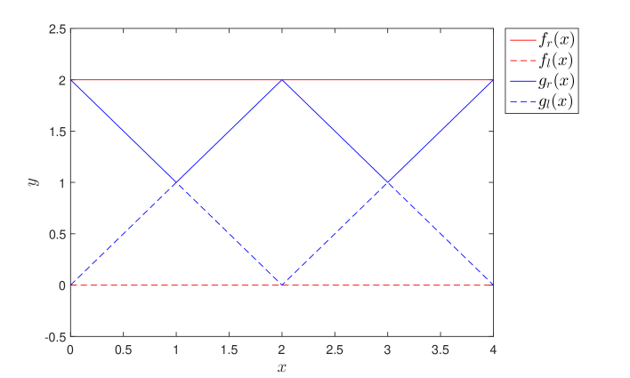
Figure 1: IVFs $\overline{f}$ and $\overline{g}$ in Example 6.12

Definition 3.3.

Let $\overline{f}:[a,b]\to\mathbb{R}_{\mathcal{I}}$, $g:[a,b]\to\mathbb{R}$, we define

$$\overline{f}(x)\star g(x):=\overline{f}(x)\star(\overline{1}~g(x)),\qquad x\in[a,b],$$

$$g(x)\star\overline{f}(x):=(\overline{1}~g(x))\star\overline{f}(x),\qquad x\in[a,b],$$

where $\star\in\{+,-,\times,\div\}$.

Now we introduce the continuity of IVFs.

Definition 3.4.

Let $\overline{f}:[a,b]\to\mathbb{R}_{\mathcal{I}}$ be an interval-valued function, given a point $x\in[a,b]$, if for arbitrary $\varepsilon>0$, there exists $\delta>0$ such that

$$d(\overline{f}(x),\overline{f}(y))<\varepsilon,$$

when $y\in O(x,\delta)\cap[a,b]$. Then $\overline{f}$ is called continuous at $x$. Further, $\overline{f}$ is called continuous on $[a,b]$ if $\overline{f}$ is continuous on every $x\in[a,b]$.

Denoted by $C([a,b],\mathbb{R}_{\mathcal{I}})$ the space of all continuous IVFs on $[a,b]$.

Theorem 3.5.

Let $\overline{f}:[a,b]\to\mathbb{R}_{\mathcal{I}}$ be an interval-valued function. Then $\overline{f}$ is continuous on $[a,b]$ if and only if $f_{l}$ and $f_{r}$ are continuous on $[a,b]$.

Proof.

(Sufficiency) Since $f_{l}$ and $f_{r}$ are continuous on $[a,b]$, then $f_{c}=\frac{f_{l}+f_{r}}{2}$ and $f_{w}=\frac{f_{r}-f_{l}}{2}$ are also continuous on $[a,b]$, so is $\ln f_{w}$. Let $x\in[a,b]$, then for arbitrary $\varepsilon_{1}>0$, there exists $\delta_{1}>0$ such that

$$|f_{c}(x)-f_{c}(y)|\leq\varepsilon_{1},$$

where $y\in O(x,\delta_{1})\cap[a,b]$. Also, for arbitrary $\varepsilon_{2}>0$, there exists $\delta_{2}>0$ such that

$$|\ln f_{w}(x)-\ln f_{w}(y)|\leq\varepsilon_{2},$$

where $y\in O(x,\delta_{2})\cap[a,b]$. Let $\delta=\min\{\delta_{1},\delta_{2}\}$, $\varepsilon=\max\{\varepsilon_{1},\varepsilon_{2}\}$, Thus,

$$d(\overline{f}(x),\overline{f}(y))=\sqrt{|f_{c}(x)-f_{c}(y)|^{2}+|\ln f_{w}(x)-\ln f_{w}(y)|^{2}}\leq\sqrt{\varepsilon_{1}^{2}+\varepsilon_{2}^{2}}\leq\sqrt{2}\varepsilon,$$

where $y\in O(x,\delta)\cap[a,b]$. By Definition 3.4, $\overline{f}$ is continuous on $[a,b]$.

(Necessity) Since $\overline{f}$ is continuous on $[a,b]$, for arbitrary $\varepsilon>0$, there exists $\delta>0$ such that

$$d(\overline{f}(x),\overline{f}(y))=\sqrt{|f_{c}(x)-f_{c}(y)|^{2}+|\ln f_{w}(x)-\ln f_{w}(y)|^{2}}\leq\varepsilon,~~x\in[a,b],$$

where $y\in O(x,\delta)\cap[a,b]$. Thus, $|f_{c}(x)-f_{c}(y)|\leq\varepsilon$, and $|\ln f_{w}(x)-\ln f_{w}(y)|\leq\varepsilon$, which imply $f_{c}$ and $\ln f_{w}$ are also continuous on $[a,b]$, so is $f_{w}$. Therefore, $f_{l}={f_{c}-f_{w}}$ and $f_{r}={f_{c}+f_{w}}$ are also continuous on $[a,b]$. ∎

Definition 3.6.

For any $\overline{f}\in C([a,b],\mathbb{R}_{\mathcal{I}})$, we define

$$\|\overline{f}\|_{\infty}=\max_{x\in[a,b]}\|\overline{f}(x)\|.$$

By Definition 3.6, it is easy to see that

Proposition 3.7.

Assume that $\overline{f},\overline{g}\in C([a,b],\mathbb{R}_{\mathcal{I}})$, $k\in\mathbb{R}$, then we have

• $\|\overline{f}\|_{\infty}\geq 0$, and $\|\overline{f}\|_{\infty}=0$ if and only if $\overline{f}=\overline{0}$;

• $\|k\overline{f}\|_{\infty}=|k|\|\overline{f}\|_{\infty}$;

• $\|\overline{f}+\overline{g}\|_{\infty}\leq\|\overline{f}\|_{\infty}+\|\overline{g}\|_{\infty}$.

Proof.

(1) $\|\overline{f}\|_{\infty}=\max_{x\in[a,b]}\|\overline{f}(x)\|=\max_{x\in[a,b]}\sqrt{f_{c}^{2}(x)+\ln^{2}f_{w}(x)}\geq 0.$ Thus, $\|\overline{f}\|_{\infty}=0$ if and only if $\overline{f}=\overline{0}$.

(2) $\|k\overline{f}\|_{\infty}=\max_{x\in[a,b]}\|k\overline{f}(x)\|=\max_{x\in[a,b]}\sqrt{k^{2}f_{c}^{2}(x)+k^{2}\ln^{2}f_{w}(x)}=|k|\|\overline{f}\|_{\infty}$.

(3)

$$\|\overline{f}+\overline{g}\|_{\infty} =\max_{x\in[a,b]}\sqrt{(f_{c}(x)+g_{c}(x))^{2}+(\ln f_{w}(x)+\ln g_{w}(x))^{2}}$$

$$\leq\max_{x\in[a,b]}\sqrt{\|\overline{f}\|_{\infty}^{2}+2f_{c}(x)g_{c}(x)+2\ln f_{w}(x)\ln g_{w}(x)+\|\overline{g}\|_{\infty}^{2}}$$

$$\leq\sqrt{\|\overline{f}\|_{\infty}^{2}+2\|\overline{f}\|_{\infty}\|\overline{g}\|_{\infty}+\|\overline{g}\|_{\infty}^{2}}$$

$$=\|\overline{f}\|_{\infty}+\|\overline{g}\|_{\infty}.$$

This ends the proof. ∎

According to Proposition 3.7, $\|\cdot\|_{\infty}$ is a norm on $C([a,b],\mathbb{R}_{\mathcal{I}})$, and

Lemma 3.8.

The space $C([a,b],\mathbb{R}_{\mathcal{I}})$ endowed with the norm $\|\cdot\|_{\infty}$ is a normed space.

Further, we can prove that

Theorem 3.9.

The space $C([a,b],\mathbb{R}_{\mathcal{I}})$ endowed with the norm $\|\cdot\|_{\infty}$ is a Banach space.

Proof.

The proof is similar to that of Theorem 2.50, so we omit it. ∎

4 Derivative of IVFs

In this section, we will present a new Derivative of IVFs based on the new subtraction given in Definition 2.21, and discuss its relationship with the classical derivative, the multiplicative derivative given in [BKO08], and the $gH$-derivative given in [SB09], respectively.

4.1 Basic Definition and Properties

Definition 4.1.

Suppose that the IVF $\overline{f}:[a,b]\rightarrow\mathbb{R}_{\mathcal{I}}$ and $x_{0}\in[a,b]$ and $x_{0}+h\in[a,b]$, then $\overline{f}$ is said to be differentiable at $x_{0}$ if there exists $\overline{f}^{\prime}(x_{0})\in\mathbb{R}_{\mathcal{I}}$ such that

$$\overline{f}^{\prime}(x_{0})=\lim\limits_{h\rightarrow 0}\frac{\overline{f}(x_{0}+h)-\overline{f}(x_{0})}{h}.$$ (4.1)

We say $\overline{f}$ is differentiable on $[a,b]$ if it is differentiable at each $x_{0}\in[a,b]$.

Theorem 4.2.

Let $\overline{f}:[a,b]\to\mathbb{R}_{\mathcal{I}}$ be an IVF with $\overline{f}(x)=\left\langle{f}_{c}(x);{f}_{w}(x)\right\rangle$. Then $\overline{f}$ is differentiable at $x\in[a,b]$ if and only if ${f}_{c}$ is differentiable at $x$, and ${f}_{w}$ is multiplicative differential at $x$. Moreover,

$$\overline{f}^{\prime}(x)=\left\langle{f}_{c}^{\prime}(x);{f}_{w}^{*}(x)\right\rangle,$$

where ${f}_{w}^{*}$ is the multiplicative derivative of $f_{w}$ on $[a,b]$ (see details in [BKO08]), i.e.,

$$f^{*}(x)=\lim_{h\to 0}\left(\frac{{f}(x+h)}{{f}(x)}\right)^{\frac{1}{h}}=\mathrm{e}^{(\ln f)^{\prime}(x)}.$$ (4.2)

Proof.

By Definition 4.1,

$$\lim_{h\to 0}\frac{\overline{f}\left({{x}}+h\right)-\overline{f}\left({{x}}\right)}{h} = \lim_{h\to 0}\frac{\langle f_{c}({{x}}+h);f_{w}({{x}}+h)\rangle-\langle f_{c}({{x}});f_{w}({{x}})\rangle}{h}$$

$$= \lim_{h\to 0}\left\langle\frac{f_{c}({{x}}+h)-f_{c}({{x}})}{h};\left(\frac{f_{w}(x+h)}{f_{w}({{x}})}\right)^{\frac{1}{h}}\right\rangle$$

$$= \left\langle{f}_{c}^{\prime}(x_{0});{f}_{w}^{*}(x_{0})\right\rangle.$$

This ends the proof. ∎

Remark 4.3.

Theorem 4.2 implies that the derivative of an IVF $\overline{f}$ on $[a,b]$ equals to the classical derivative of the center function $f_{c}$, and the multiplicative derivative of the radius function $f_{w}$.

Definition 4.4.

Let $\overline{F},\overline{f}:[a,b]\to\mathbb{R}_{\mathcal{I}}$, if

$$\overline{F}^{\prime}(x)=\overline{f}(x),~~x\in[a,b],$$

then $\overline{F}$ is called a primitive of $\overline{f}$ on $[a,b]$.

Proposition 4.5.

Suppose that $\overline{f},\overline{g}:[a,b]\to\mathbb{R}_{\mathcal{I}}$ are differentiable on $[a,b]$. Then for any $x\in[a,b]$,

• ${{\left(c_{1}\overline{f}+c_{2}\overline{g}\right)}{{}^{\prime}}}\left({{x}}\right)=c_{1}{{\overline{f}}{{}^{\prime}}}\left({{x}}\right)+c_{2}{{\overline{g}}{{}^{\prime}}}\left({{x}}\right),$ where $c_{1},c_{2}\in\mathbb{R}_{\mathcal{I}}.$

• $(\overline{f}~\overline{g})^{\prime}(x)=\overline{f}^{\prime}(x)\overline{g}(x)+\overline{f}(x)\overline{g}^{\prime}(x).$

• $\left(\frac{~\overline{f}~}{\overline{g}}\right)^{\prime}(x)=\displaystyle\frac{\overline{f}^{\prime}(x)\overline{g}(x)-\overline{f}(x)\overline{g}^{\prime}(x)}{\overline{g}^{2}(x)}.$

Proof.

(1)

$${{\left(c_{1}\overline{f}+c_{2}\overline{g}\right)}{{}^{\prime}}}\left({{x}}\right) = \lim_{h\to 0}\frac{(c_{1}\overline{f}(x_{0}+h)+c_{2}\overline{g}(x_{0}+h))-(c_{1}\overline{f}(x_{0})+c_{2}\overline{g}(x_{0}))}{h}$$

$$= \lim_{h\to 0}\left(c_{1}\frac{\overline{f}(x_{0}+h)-\overline{f}(x_{0})}{h}+c_{2}\frac{\overline{g}(x_{0}+h)-\overline{g}(x_{0})}{h}\right)$$

$$= c_{1}{{\overline{f}}{{}^{\prime}}}\left({{x}}\right)+c_{2}{{\overline{g}}{{}^{\prime}}}\left({{x}}\right).$$

(2)

$${{\left(\overline{f}(x)\overline{g}\right)}{{}^{\prime}}}\left({{x}}\right) = \langle f_{c}(x)g_{c}(x);\mathrm{e}^{\ln f_{w}(x)\ln g_{w}(x)}\rangle^{\prime}$$

$$= \langle f_{c}^{\prime}(x)g_{c}(x)+f_{c}(x_{0})g_{c}^{\prime}(x);\mathrm{e}^{(\ln f_{w})^{\prime}(x)\ln g_{w}(x)+\ln f_{w}(x)(\ln g_{w})^{\prime}(x)}\rangle$$

$$= \langle f_{c}^{\prime}(x)g_{c}(x);\mathrm{e}^{\ln f_{w}^{\prime}(x)\ln g_{w}(x)}\rangle+\langle f_{c}(x)g_{c}^{\prime}(x);\mathrm{e}^{\ln f_{w}(x)(\ln g_{w})(x)}\rangle$$

$$= \langle f_{c}^{\prime}(x);f_{w}^{*}(x)\rangle\langle g_{c}(x);g_{w}(x)\rangle+\langle f_{c}(x);f_{w}(x)\rangle\langle g_{c}^{\prime}(x);g_{w}^{*}(x)\rangle$$

$$= \overline{f}^{\prime}(x)\overline{g}(x)+\overline{f}(x)\overline{g}^{\prime}(x).$$

(3)

$$\left(\frac{~\overline{f}~}{\overline{g}}\right)^{\prime}(x)= \lim_{h\to 0}\frac{\frac{\overline{f}(x+h)}{\overline{g}(x+h)}-\frac{\overline{f}(x)}{\overline{g}(x)}}{h}$$

$$= \lim_{h\to 0}\left\langle\frac{\frac{f_{c}(x+h)}{g_{c}(x+h)}-\frac{f_{c}(x)}{g_{c}(x)}}{h};\mathrm{e}^{\frac{1}{h}\left(\frac{\ln f_{w}(x+h)}{\ln g_{w}(x+h)}-\frac{\ln f_{w}(x)}{\ln g_{w}(x)}\right)}\right\rangle$$

$$= \left\langle\frac{{f_{c}^{\prime}(x)}{g_{c}(x)}-{f_{c}(x)}{g_{c}^{\prime}(x)}}{g_{c}^{2}(x)};\mathrm{e}^{\frac{{(\ln f_{w})^{\prime}(x)}{\ln g_{w}(x)}-{\ln f_{w}(x)}{(\ln g_{w})^{\prime}(x)}}{(\ln g_{w}(x))^{2}}}\right\rangle$$

$$= \frac{\left\langle{{f_{c}^{\prime}(x)}{g_{c}(x)}-{f_{c}(x)}{g_{c}^{\prime}(x)}};\mathrm{e}^{{{(\ln f_{w})^{\prime}(x)}{\ln g_{w}(x)}-{\ln f_{w}(x)}{(\ln g_{w})^{\prime}(x)}}}\right\rangle}{\overline{g}^{2}(x)}$$

$$= \frac{\left\langle f_{c}^{\prime}(x)g_{c}(x);\mathrm{e}^{(\ln f_{w})^{\prime}(x)\ln g_{w}(x)}\right\rangle-\left\langle f_{c}(x)g_{c}^{\prime}(x);\mathrm{e}^{\ln f_{w}(x)(\ln g_{w})^{\prime}(x)}\right\rangle}{\overline{g}^{2}(x)}$$

$$= \frac{\overline{f}^{\prime}(x)\overline{g}(x)-\overline{f}(x)\overline{g}^{\prime}(x)}{\overline{g}(x)^{2}}.$$

The proof is therefore ended. ∎

Corollary 4.6.

Suppose that $\overline{f}:[a,b]\to\mathbb{R}_{\mathcal{I}}$ are differentiable on $[a,b]$, and that $g:[a,b]\to\mathbb{R}$ is differentiable on $[a,b]$. Then for any $x\in[a,b]$,

1. ${{\left(c_{1}\overline{f}+c_{2}g\right)}{{}^{\prime}}}\left({{x}}\right)=c_{1}{{\overline{f}}{{}^{\prime}}}\left({{x}}\right)+c_{2}{{g}{{}^{\prime}}}\left({{x}}\right),$ where $c_{1},c_{2}\in\mathbb{R}_{\mathcal{I}}.$

2. $(\overline{f}~g)^{\prime}(x)=\overline{f}^{\prime}(x)g(x)+\overline{f}(x)g^{\prime}(x).$

3. $\left(\frac{~\overline{f}~}{g}\right)^{\prime}(x)=\displaystyle\frac{\overline{f}^{\prime}(x)g(x)-\overline{f}(x)g^{\prime}(x)}{g^{2}(x)}.$

4. $\left(\frac{~g~}{\overline{f}}\right)^{\prime}(x)=\displaystyle\frac{g^{\prime}(x)\overline{f}(x)-g(x)\overline{f}^{\prime}(x)}{\overline{f}^{2}(x)}.$

Proof.

This is a direct conclusion of Proposition 4.5 and Definition 3.3. ∎

Theorem 4.7.

Suppose that $\overline{f}:[a,b]\to\mathbb{R}_{\mathcal{I}}$ is differentiable on $[a,b]$. Then for any $x\in[a,b]$,

$${{\left(\overline{f}\circ g\right)}{{}^{\prime}}}\left({{x}}\right)={{\overline{f}}{{}^{\prime}}}\left({{y}}\right){{g}{{}^{\prime}}}\left({{x}}\right),$$

where $g:[a,b]\to[a,b]$ is differentiable, and ${{y}}=g\left({{x}}\right)$.

Proof.

$$\left(\overline{f}\circ g\right)^{\prime}\left(x\right)= \lim_{h\to 0}\frac{\overline{f}(g(x+h))-\overline{f}(g(x))}{h}$$

$$= \lim_{h\to 0}\left\langle\frac{f_{c}(g(x+h))-f_{c}(g(x))}{h};\left(\frac{f_{w}(g(x+h))}{f_{w}(g(x))}\right)^{\frac{1}{h}}\right\rangle$$

$$= \left\langle f_{c}^{\prime}(y)g^{\prime}(x);\mathrm{e}^{\frac{f_{w}^{\prime}(y)}{f_{w}(y)}g^{\prime}(x)}\right\rangle$$

$$= {{\overline{f}}{{}^{\prime}}}\left({{y}}\right){{g}{{}^{\prime}}}\left({{x}}\right).$$

This ends the proof. ∎

Theorem 4.8.

Let $\overline{f}:[a,b]\to\mathbb{R}_{\mathcal{I}}$ be an interval-valued function. If $\overline{f}$ is differentiable on $[a,b]$, then $\overline{f}$ is continuous on $[a,b]$.

Proof.

Since $\overline{f}$ is differentiable on $[a,b]$, then by Theorem 4.2,

$$\overline{f}^{\prime}\left(x\right)=\left\langle{f}_{c}^{\prime}(x);{f}_{w}^{*}(x)\right\rangle.$$

From (4.2), it follows that

$${f}_{w}^{*}(x)=\mathrm{e}^{(\ln f_{w})^{\prime}(x)}=\mathrm{e}^{\frac{f_{w}^{\prime}(x)}{f_{w}(x)}},$$

which implies that $f_{w}$ is differentiable on $[a,b]$. Hence, $f_{l}=f_{c}-f_{w}$ and $f_{r}=f_{c}+f_{w}$ are also differentiable on $[a,b]$. Thus, $f_{l}$ and $f_{r}$ are continuous on $[a,b]$, by Theorem 3.5, so is $\overline{f}$. ∎

4.2 Comparison with the $gH$-Derivative

Now we discuss the relationship between the new derivative and the $gH$-derivative.

Theorem 4.9.

Let $\overline{f}:[a,b]\to\mathbb{R}_{\mathcal{I}}$ be an IVF. If $\overline{f}$ is continuous on $[a,b]$, then $\overline{f}$ is differentiable on $[a,b]$ if and only if $\overline{f}$ is $gH$-differentiable on $[a,b]$.

Proof.

(Necessity) Since $\overline{f}$ is differentiable on $[a,b]$, it follows from the proof of Theorem 4.8 that $f_{l}=f_{c}-f_{w}$ and $f_{r}=f_{c}+f_{w}$ are also differentiable on $[a,b]$. Thus, by [SB09, Theorem 17], $\overline{f}$ is $gH$-differentiable on $[a,b]$.

(Sufficiency) The sufficiency is obvious according to the necessity. ∎

Example 4.10.

Let us consider the function $\overline{f}:\mathbb{R}\rightarrow\mathbb{R}_{\mathcal{I}}$,

$$\overline{f}(x)=\left\{\begin{array}[]{ll}{[0,1]}\Big(1-x^{2}\sin\frac{1}{x}\Big),\quad&\text{if}~x\not=0;\\ {[0,1]},&\text{otherwise}.\end{array}\right.$$

Since

$$\overline{f}_{gH}^{\prime}(x)=\lim\limits_{h\rightarrow 0}\frac{\overline{f}(h)\ominus_{gH}\overline{f}(0)}{h}= \lim\limits_{h\rightarrow 0}\frac{{[0,1]}\Big(1-h^{2}\sin\frac{1}{h}\Big)\ominus_{gH}[0,1]}{h}$$

$$= \lim\limits_{h\rightarrow 0}{\left[\min\left\{0,-h\sin\frac{1}{h}\right\},\max\left\{0,-h\sin\frac{1}{h}\right\}\right]}$$

$$= 0,$$

$\overline{f}$ is differentiable at $x_{0}=0$ and $\overline{f}_{gH}^{\prime}(0)=0$. But,

$$\overline{f}^{\prime}(x)=\lim\limits_{h\rightarrow 0}\frac{\overline{f}(h)-\overline{f}(0)}{h}= \lim\limits_{h\rightarrow 0}\left\langle\frac{-h\sin\frac{1}{h}}{2};\left(\frac{1}{2}\right)^{{(-h\sin\frac{1}{h})}}\right\rangle$$

$$= \langle 0;1\rangle$$

$$= [-1,1].$$

Example 4.11.

Let us consider the function $f:\mathbb{R}\rightarrow\mathbb{R}_{\mathcal{I}}$,

$$f(x)=[-|x|,|x|+1].$$

Since

$$\lim\limits_{h\rightarrow 0}\frac{\overline{f}(h)-\overline{f}(0)}{h}= \lim\limits_{h\rightarrow 0}\frac{\langle\frac{1}{2},|h|+\frac{1}{2}\rangle-\langle\frac{1}{2};\frac{1}{2}\rangle}{h}$$

$$= \lim\limits_{h\rightarrow 0}{\langle 0,\left(2|h|+1\right)^{\frac{1}{h}}\rangle}$$

$$= \begin{cases}\langle 0,\mathrm{e}^{2}\rangle,&\text{ if }h>0,\\ \langle 0,\mathrm{e}^{-2}\rangle,&\text{ if }h<0,\end{cases},$$

so, $\overline{f}$ is not differentiable at $x_{0}=0$. However, $f_{l}$ and $f_{r}$ are both not differentiable at $x=0$, so $\overline{f}$ is neither not $gH$-differentiable at $x=0$.

Remark 4.12.

Theorem 4.9 is not true, if the condition that $\overline{f}$ is continuous on $[a,b]$ is omitted, see the counterexample 4.13.

Example 4.13.

[QD] Consider the IVF $f:\mathbb{R}\rightarrow\mathbb{R}_{\mathcal{I}}$ as follows,

$$\overline{f}(x)=\left\{\begin{array}[]{ll}{[-1,x^{2}+x]}\,\,\,\,\,\,\text{if}~x\in\mathbb{Q};\\ {[x-1,x^{2}]},\,\,\,\,\,\,\,\,\text{if}~x\in\mathbb{R}\setminus\mathbb{Q}.\end{array}\right.$$

If $h\in\mathbb{Q}$, then

$$\lim\limits_{h\rightarrow 0}\frac{\overline{f}(h)-\overline{f}(0)}{h}= \lim\limits_{h\rightarrow 0}\frac{{[-1,h^{2}+h]}-[-1,0]}{h}$$

$$= \lim\limits_{h\rightarrow 0}\left\langle\frac{h+1}{2};(h^{2}+h+1)^{\frac{1}{h}}\right\rangle$$

$$= \left\langle\frac{1}{2};\mathrm{e}\right\rangle.$$

If $h\in\mathbb{R}\setminus\mathbb{Q}$, then

$$\lim\limits_{h\rightarrow 0}\frac{\overline{f}(h)-\overline{f}(0)}{h}= \lim\limits_{h\rightarrow 0}\frac{{[h-1,h^{2}]}-[-1,0]}{h}$$

$$= \lim\limits_{h\rightarrow 0}\left\langle\frac{h+1}{2};(h^{2}-h+1)^{\frac{1}{h}}\right\rangle$$

$$= \left\langle\frac{1}{2};\mathrm{e}^{-1}\right\rangle.$$

Hence, $f$ is not differentiable at $x_{0}=0$.

On the other hand, $\overline{f}$ is gH-differentiable at $x_{0}=0$ and $\overline{f}^{\prime}_{gH}(0)=[0,1]$.

Remark 4.14.

It is worth noting that when calculating the $gH$-derivative, the issue of the function’s switching points needs to be considered, see [SB09]. However, the new derivative proposed in Definition 4.1 does not have this issue, thus the complexity of the calculation is significantly reduced.

Example 4.15.

Considering the IVF $\overline{f}(x)=\left[\frac{1}{2}x^{2},1+\frac{1}{2}x^{2}+2\sin^{2}x\right],$ $x\in[0,2\pi]$. If we calculate the $gH$-derivative $\overline{f}^{\prime}_{gH}(x)=[f^{\prime}_{l~gH}(x),f^{\prime}_{r~gH}(x)]$, it has three switching points $x_{1}=\frac{1}{2}\pi$, $x_{2}=\pi$ and $x_{3}=\frac{3}{2}\pi$. However,

$$\overline{f}^{\prime}(x)=[f^{\prime}_{l}(x),f^{\prime}_{r}(x)]=\left[x+\sin 2x-\mathrm{e}^{\frac{2\sin 2x}{2-\cos 2x}},x+\sin 2x+\mathrm{e}^{\frac{2\sin 2x}{2-\cos 2x}}\right],\quad x\in[0,2\pi],$$

see Figure 2.

(a) $\overline{f}(x)$

(b) $\overline{f}^{\prime}_{gH}(x)$ and $\overline{f}^{\prime}(x)$

Figure 2: The IVF $\overline{f}(x)$ in Example 4.15 and its derivatives

5 Integration of IVFs

In this subsection, we will introduce the concept of Riemann type integrals of interval-valued functions and its properties.

5.1 Basic Definition and Properties

Definition 5.1.

Let $\overline{f}:\left[a,b\right]\to{{\mathbb{R}}_{\mathcal{I}}},\overline{A}\in{{\mathbb{R}}_{\mathcal{I}}}$. If for arbitrary $\varepsilon>0$, there exists a constant $\delta>0$ such that for any division $P$ of $\left[a,b\right]$ given by

$$a={{t}_{0}}<{{t}_{1}}<{{t}_{2}}<\cdots<{{t}_{n-1}}<{{t}_{n}}=b,\text{ and }(\xi_{1},\xi_{2},...,\xi_{n})$$

satisfies $t_{i-1}\leq\xi_{i}\leq t_{i}$ and $t_{i}-t_{i-1}<\delta$ for all $i$, one has

$$d\left(\sum_{i=1}^{n}{\overline{f}\left({{\xi}_{i}}\right)\left({{t}_{i}}-{{t}_{i-1}}\right)},\overline{A}\right)<\varepsilon.$$

Then $\overline{f}$ is said to be interval Riemann integrable to $\overline{A}$ on $\left[a,b\right]$, and denoted by

$$\overline{A}=\left(IR\right)\int_{a}^{b}{\overline{f}\left(t\right)}\operatorname{d}t.$$

Denote by $\mathcal{IR}([a,b],\mathbb{R}_{\mathcal{I}})$ the space of all interval Riemann integrable IVFs $\overline{f}$ on $[a,b]$. Also, denote by $\mathcal{R}([a,b],\mathbb{R})$ the space of all Riemann integrable funcitons $f$ on $[a,b]$.

Theorem 5.2.

Suppose that $\overline{f}:\left[a,b\right]\to{{\mathbb{R}}_{\mathcal{I}}}$ with $\overline{f}\left(t\right)=\left\langle{f}_{c}\left(t\right),{f}_{w}\left(t\right)\right\rangle,t\in\left[a,b\right]$, then $\overline{f}\in\mathcal{I}\mathcal{R}\left(\left[a,b\right],\mathbb{R}_{\mathcal{I}}\right)$ if and only if ${f}_{c},\ln{f}_{w}\in\mathcal{R}\left(\left[a,b\right],\mathbb{R}\right)$. Moreover,

$$\left(IR\right)\int_{a}^{b}{\overline{f}\left(t\right)}\operatorname{d}t=\left\langle\left(R\right)\int_{a}^{b}{{f}_{c}\left(t\right)}\operatorname{d}t;\left(R\right)\int_{a}^{b}{{f}_{w}\left(t\right)}^{\operatorname{d}t}\right\rangle,$$

where $\left(R\right)\int_{a}^{b}{{f}_{w}\left(t\right)}^{\operatorname{d}t}$ is the multiplication integral of ${f}_{w}$ on $[a,b]$ (see details in [BKO08]), i.e.,

$$(R)\int_{a}^{b}{{f}_{w}\left(t\right)}^{\operatorname{d}t}=\mathrm{e}^{(R)\int_{a}^{b}(\ln f_{w})(t)\operatorname{d}t}.$$ (5.1)

Proof.

By Definition 4.1, one has

$$\left(IR\right)\int_{a}^{b}{\overline{f}\left(t\right)}\operatorname{d}t = \lim_{\delta\to 0}\sum\limits_{i=1}^{n}{\overline{f}\left({{\xi}_{i}}\right)\left({{t}_{i}}-{{t}_{i-1}}\right)}$$

$$= \lim_{\delta\to 0}\sum\limits_{i=1}^{n}{\langle f_{c}\left({{\xi}_{i}}\right);f_{w}(\xi_{i})\rangle\left({{t}_{i}}-{{t}_{i-1}}\right)}$$

$$= \lim_{\delta\to 0}{\left\langle\sum\limits_{i=1}^{n}f_{c}\left({{\xi}_{i}}\right)\left({{t}_{i}}-{{t}_{i-1}}\right);\prod_{i=1}^{n}f_{w}(\xi_{i})^{\left({{t}_{i}}-{{t}_{i-1}}\right)}\right\rangle}$$

$$= \lim_{\delta\to 0}{\left\langle\sum\limits_{i=1}^{n}f_{c}\left({{\xi}_{i}}\right)\left({{t}_{i}}-{{t}_{i-1}}\right);\mathrm{e}^{\sum\limits_{i=1}^{n}\ln f_{w}(\xi_{i}){\left({{t}_{i}}-{{t}_{i-1}}\right)}}\right\rangle}$$

$$= \left\langle\left(R\right)\int_{a}^{b}{{f}_{c}\left(t\right)}\operatorname{d}t;\mathrm{e}^{(R)\int_{a}^{b}(\ln f_{w})(t)\operatorname{d}t}\right\rangle,$$

$$= \left\langle\left(R\right)\int_{a}^{b}{{f}_{c}\left(t\right)}\operatorname{d}t;\left(R\right)\int_{a}^{b}{{f}_{w}\left(t\right)}^{\operatorname{d}t}\right\rangle.$$

This ends the proof. ∎

Theorem 5.3.

Suppose that $\overline{f}\in C(\left[a,b\right],{{\mathbb{R}}_{\mathcal{I}}})$, then $\overline{f}\in\mathcal{I}\mathcal{R}\left(\left[a,b\right],\mathbb{R}_{\mathcal{I}}\right)$.

Proof.

Since $\overline{f}\in C(\left[a,b\right],{{\mathbb{R}}_{\mathcal{I}}})$, by Theorem 3.5, $f_{l}$ and $f_{r}$ are continuous on $[a,b]$, so are $f_{c}$ and $f_{w}$. Hence, $f_{c}$ and $\ln f_{w}$ are integrable on $[a,b]$. From Theorem 5.2, it follows that $\overline{f}\in\mathcal{I}\mathcal{R}\left(\left[a,b\right],\mathbb{R}_{\mathcal{I}}\right)$. ∎

The interval Riemann integral has the following properties.

Proposition 5.4.

(1) (Monotonicity). Suppose that $\overline{f},\overline{g}\in\mathcal{I}\mathcal{R}\left(\left[a,b\right],\mathbb{R}_{\mathcal{I}}\right)$. If $\overline{f}\left(t\right)\leq\overline{g}\left(t\right)$ for any $t\in\left[a,b\right]$, then

$$\left(IR\right)\int_{a}^{b}{\overline{f}\left(t\right)}\operatorname{d}t\leq\left(IR\right)\int_{a}^{b}{\overline{g}\left(t\right)}\operatorname{d}t.$$

(2) (Linearity). Suppose that $\overline{f},\overline{g}\in\mathcal{I}\mathcal{R}\left(\left[a,b\right],\mathbb{R}_{\mathcal{I}}\right),\lambda_{1},\lambda_{2}\in\mathbb{R}_{\mathcal{I}}$, then $\lambda_{1}\overline{f}+\lambda_{2}\overline{g}\in\mathcal{I}\mathcal{R}\left(\left[a,b\right],\mathbb{R}_{\mathcal{I}}\right)$, and

$$\left(IR\right)\int_{a}^{b}{\left[\lambda_{1}\overline{f}\left(t\right)\ +\lambda_{2}\overline{g}\left(t\right)\right]}\operatorname{d}t=\lambda_{1}\left(IR\right)\int_{a}^{b}{\overline{f}\left(t\right)}\operatorname{d}t+\lambda_{2}\left(IR\right)\int_{a}^{b}{\overline{g}\left(t\right)}\operatorname{d}t.$$

(3) (Subinterval Integrability). If IVF $\overline{f}\in\mathcal{I}\mathcal{R}\left(\left[a,b\right],\mathbb{R}_{\mathcal{I}}\right)$, then so it is on a subinterval $\left[c,d\right]\subseteq\left[a,b\right]$.

(4) (Additivity). Suppose that $\overline{f}\in\mathcal{I}\mathcal{R}\left(\left[a,b\right],\mathbb{R}_{\mathcal{I}}\right)$, then for any $c\in\left[a,b\right]$, it holds

$$\left(IR\right)\int_{a}^{b}{\overline{f}\left(t\right)}\operatorname{d}t=\left(IR\right)\int_{a}^{c}{\overline{f}\left(t\right)}\operatorname{d}t+\left(IR\right)\int_{c}^{b}{\overline{f}\left(t\right)}\operatorname{d}t.$$

Proof.

(1) By Definition 2.1, there are three cases in “$\leq$”.

(I) If $\overline{f}\left(t\right)=\overline{g}\left(t\right)$, $t\in[a,b]$, then it is easy to see that

$$\left(IR\right)\int_{a}^{b}{\overline{f}\left(t\right)}\operatorname{d}t=\left(IR\right)\int_{a}^{b}{\overline{g}\left(t\right)}\operatorname{d}t.$$

(II) If $f_{c}\left(t\right)<g_{c}\left(t\right)$, $t\in[a,b]$, then one has

$$\left(R\right)\int_{a}^{b}{f_{c}\left(t\right)}\operatorname{d}t<\left(R\right)\int_{a}^{b}{g_{c}\left(t\right)}\operatorname{d}t,$$

that is,

$$\left(IR\right)\int_{a}^{b}{\overline{f}\left(t\right)}\operatorname{d}t\leq\left(IR\right)\int_{a}^{b}{\overline{g}\left(t\right)}\operatorname{d}t.$$

(III) If $f_{c}\left(t\right)=g_{c}\left(t\right)$, $f_{w}\left(t\right)<g_{w}\left(t\right)$, $t\in[a,b]$, then we have

$$\left(R\right)\int_{a}^{b}{\ln f_{w}\left(t\right)}\operatorname{d}t<\left(R\right)\int_{a}^{b}{\ln g_{w}\left(t\right)}\operatorname{d}t,$$

by (5.1), it holds

$$\left(IR\right)\int_{a}^{b}{\overline{f}\left(t\right)}\operatorname{d}t\leq\left(IR\right)\int_{a}^{b}{\overline{g}\left(t\right)}\operatorname{d}t.$$

(2) Since $\overline{f},\overline{g}\in\mathcal{I}\mathcal{R}\left(\left[a,b\right],\mathbb{R}_{\mathcal{I}}\right)$, by Lemma 5.2, the functions $f_{c},\ln f_{w},g_{c},\ln g_{w}\in\mathcal{R}\left(\left[a,b\right],\mathbb{R}_{\mathcal{I}}\right),$ so are $\lambda_{1}f_{c}+\lambda_{2}g_{c}$ and $\lambda_{1}\ln f_{w}+\lambda_{2}\ln g_{w}$. Then

$$\lambda_{1}\overline{f}+\lambda_{2}\overline{g}=\left\langle\lambda_{1}f_{c}+\lambda_{2}g_{c};\mathrm{e}^{\lambda_{1}\ln f_{w}+\lambda_{2}\ln g_{w}}\right\rangle\in\mathcal{I}\mathcal{R}\left(\left[a,b\right],\mathbb{R}_{\mathcal{I}}\right).$$

Moreover,

$$\left(IR\right)\int_{a}^{b}{\left[\lambda_{1}\overline{f}\left(t\right)\ +\lambda_{2}\overline{g}\left(t\right)\right]}\operatorname{d}t$$

$$= (IR)\int_{a}^{b}\left\langle\lambda_{1}f_{c}(t)+\lambda_{2}g_{c}(t);\mathrm{e}^{\lambda_{1}\ln f_{w}(t)+\lambda_{2}\ln g_{w}(t)}\right\rangle\operatorname{d}t$$

$$= \left\langle(R)\int_{a}^{b}\lambda_{1}f_{c}(t)+\lambda_{2}g_{c}(t)\operatorname{d}t;\mathrm{e}^{(R)\int_{a}^{b}\lambda_{1}\ln f_{w}(t)+\lambda_{2}\ln g_{w}(t)\operatorname{d}t}\right\rangle$$

$$= \left\langle\lambda_{1}(R)\int_{a}^{b}f_{c}(t)\operatorname{d}t+\lambda_{2}(R)\int_{a}^{b}g_{c}(t)\operatorname{d}t;\mathrm{e}^{\lambda_{1}(R)\int_{a}^{b}\ln f_{w}(t)\operatorname{d}t+\lambda_{2}(R)\int_{a}^{b}\ln g_{w}(t)\operatorname{d}t}\right\rangle$$

$$= \left\langle\lambda_{1}(R)\int_{a}^{b}f_{c}(t)\operatorname{d}t;\mathrm{e}^{\lambda_{1}(R)\int_{a}^{b}\ln f_{w}(t)\operatorname{d}t}\right\rangle+\left\langle\lambda_{2}(R)\int_{a}^{b}g_{c}(t)\operatorname{d}t;\mathrm{e}^{\lambda_{2}(R)\int_{a}^{b}\ln g_{w}(t)\operatorname{d}t}\right\rangle$$

$$= \lambda_{1}\left(IR\right)\int_{a}^{b}{\overline{f}\left(t\right)}\operatorname{d}t+\lambda_{2}\left(IR\right)\int_{a}^{b}{\overline{g}\left(t\right)}\operatorname{d}t.$$

(3) Since $\overline{f}\in\mathcal{I}\mathcal{R}\left(\left[a,b\right],\mathbb{R}_{\mathcal{I}}\right)$, by Lemma 5.2, the functions $f_{c},\ln f_{w}\in\mathcal{R}\left(\left[a,b\right],\mathbb{R}_{\mathcal{I}}\right).$ Hence, for any $[c,d]\subseteq[a,b]$, the functions $f_{c},\ln f_{w}\in\mathcal{R}\left(\left[c,d\right],\mathbb{R}_{\mathcal{I}}\right)$, thereby, $\overline{f}\in\mathcal{I}\mathcal{R}\left(\left[c,d\right],\mathbb{R}_{\mathcal{I}}\right)$.

(4) Since $\overline{f}\in\mathcal{I}\mathcal{R}\left(\left[a,b\right],\mathbb{R}_{\mathcal{I}}\right)$, by Lemma 5.2, the functions $f_{c},\ln f_{w}\in\mathcal{R}\left(\left[a,b\right],\mathbb{R}_{\mathcal{I}}\right).$ Hence, for any $c\in[a,b]$, the functions $f_{c},\ln f_{w}\in\mathcal{R}\left(\left[a,c\right],\mathbb{R}_{\mathcal{I}}\right)$, and also $f_{c},\ln f_{w}\in\mathcal{R}\left(\left[c,b\right],\mathbb{R}_{\mathcal{I}}\right)$, thereby,

$$\left(IR\right)\int_{a}^{b}{\overline{f}\left(t\right)}\operatorname{d}t$$

$$= \left\langle(R)\int_{a}^{b}f_{c}(t)\operatorname{d}t;\mathrm{e}^{(R)\int_{a}^{b}\ln f_{w}(t)\operatorname{d}t}\right\rangle$$

$$= \left\langle(R)\int_{a}^{c}f_{c}(t)\operatorname{d}t+(R)\int_{c}^{b}f_{c}(t)\operatorname{d}t;\mathrm{e}^{(R)\int_{a}^{c}\ln f_{w}(t)\operatorname{d}t+(R)\int_{c}^{b}\ln f_{w}(t)\operatorname{d}t}\right\rangle$$

$$= \left\langle(R)\int_{a}^{c}f_{c}(t)\operatorname{d}t;\mathrm{e}^{(R)\int_{a}^{c}\ln f_{w}(t)\operatorname{d}t}\right\rangle+\left\langle(R)\int_{c}^{b}f_{c}(t)\operatorname{d}t;\mathrm{e}^{(R)\int_{c}^{b}\ln f_{w}(t)\operatorname{d}t}\right\rangle$$

$$= \left(IR\right)\int_{a}^{c}{\overline{f}\left(t\right)}\operatorname{d}t+\left(IR\right)\int_{c}^{b}{\overline{f}\left(t\right)}\operatorname{d}t.$$

This ends the proof. ∎

By Proposition 5.4 and Definition 3.3, we have

Corollary 5.5.

Suppose that $\overline{f}\in\mathcal{I}\mathcal{R}\left(\left[a,b\right],\mathbb{R}_{\mathcal{I}}\right)$ and $g\in\mathcal{R}\left(\left[a,b\right],\mathbb{R}\right),$ $\lambda_{1},\lambda_{2}\in\mathbb{R}_{\mathcal{I}}$, then $\lambda_{1}\overline{f}+\lambda_{2}g\in\mathcal{I}\mathcal{R}\left(\left[a,b\right],\mathbb{R}_{\mathcal{I}}\right)$, and

$$\left(IR\right)\int_{a}^{b}{\left[\lambda_{1}\overline{f}\left(t\right)\ +\lambda_{2}g\left(t\right)\right]}\operatorname{d}t=\lambda_{1}\left(IR\right)\int_{a}^{b}{\overline{f}\left(t\right)}\operatorname{d}t+\lambda_{2}\left(R\right)\int_{a}^{b}{g\left(t\right)}\operatorname{d}t.$$

5.2 Fundamental Theorem of Calculus

Theorem 5.6.

Let $\overline{f}\in\mathcal{IR}([a,b],\mathbb{R}_{\mathcal{I}})$, if $\overline{F}:[a,b]\to\mathbb{R}_{\mathcal{I}}$ is given by

$$\overline{F}(t)=(IR)\int_{a}^{t}\overline{f}(s)\operatorname{d}s,~~t\in[a,b],$$

then $\overline{F}$ is continuous on $[a,b]$ and $\overline{F}^{\prime}=\overline{f}$ at all points of continuity of $\overline{f}$.

Proof.

Since $\overline{f}\in\mathcal{I}\mathcal{R}\left(\left[a,b\right],\mathbb{R}_{\mathcal{I}}\right)$, and

$$\overline{F}(t)=(IR)\int_{a}^{t}\overline{f}(s)\operatorname{d}s,~~t\in[a,b],$$

then for any $t_{1},t_{2}\in[a,b]$,

$$d(\overline{F}(t_{1}),\overline{F}(t_{2}))= d\left((IR)\int_{a}^{t_{1}}\overline{f}(s)\operatorname{d}s,(IR)\int_{a}^{t_{2}}\overline{f}(s)\operatorname{d}s\right)$$

$$= \sqrt{\left((R)\int_{t_{2}}^{t_{1}}f_{c}(s)\operatorname{d}s\right)^{2}+\left((R)\int_{t_{2}}^{t_{1}}\ln f_{w}(s)\operatorname{d}s\right)^{2}}$$

$$\to 0,\text{ as }t_{1}\to t_{2},$$

so $\overline{F}$ is continuous on $[a,b]$.

Moreover, for any point $x$ of continuity of $\overline{f}$ and $x+h\in[a,b]$,

$$\overline{F}^{\prime}(x)= \lim_{h\to 0}\frac{\overline{F}(x+h)-\overline{F}(x)}{h}$$

$$= \lim_{h\to 0}\frac{(IR)\int_{x}^{x+h}\overline{f}(s)\operatorname{d}s}{h}$$

$$= \lim_{h\to 0}\overline{f}(\xi)$$

$$= \overline{f}(x).$$

This ends the proof. ∎

Theorem 5.7.

Assume that $\overline{f}\in C([a,b],\mathbb{R}_{\mathcal{I}})$. If $\overline{F}$ is a primitive of $\overline{f}$ on $[a,b]$, then

$$\overline{F}(b)-\overline{F}(a)=(IR)\int_{a}^{b}\overline{f}(t)\operatorname{d}t.$$ (5.2)

Proof.

Since $\overline{f}\in C([a,b],\mathbb{R}_{\mathcal{I}})$, by Theorem 5.6, $(IR)\int_{a}^{t}\overline{f}(s)\operatorname{d}s$ is a primitive of $\overline{f}$ on $[a,b]$. This and the fact that $\overline{F}$ is a primitive of $\overline{f}$ on $[a,b]$ imply that

$$F(t)=(IR)\int_{a}^{t}\overline{f}(s)\operatorname{d}s+\overline{C},~~t\in[a,b],~~\overline{C}\in\mathbb{R}_{\mathcal{I}}.$$ (5.3)

Taking $t=a$ and $t=b$ in (5.3), on has

$$\overline{F}(b)-\overline{F}(a)=(IR)\int_{a}^{b}\overline{f}(t)\operatorname{d}t.$$

The proof is therefore completed. ∎

The following example shows that (5.2) is strict.

Example 5.8.

Considering that $\overline{F}(t)=[t,t^{2}+1]$, $t\in[0,1]$. By Theorem 4.2, we have

$$\overline{F}^{\prime}(t)=\left\langle t+\frac{1}{2};\mathrm{e}^{\frac{2t-1}{t^{2}-t+1}}\right\rangle,~~t\in[0,1].$$

Due to Theorem 5.2, one has

$$(IR)\int_{0}^{1}\overline{F}^{\prime}(t)\operatorname{d}t= (IR)\int_{0}^{1}\left\langle t+\frac{1}{2};\mathrm{e}^{\frac{2t-1}{t^{2}-t+1}}\right\rangle\operatorname{d}t$$

$$= \left\langle 1;1\right\rangle$$

$$= [0.2].$$

On the other hand,

$$\overline{F}(1)-\overline{F}(0)=[1,2]-[0,1]=[0,2].$$

Hence,

$$\overline{F}(1)-\overline{F}(0)=(IR)\int_{0}^{1}\overline{F}^{\prime}(t)\operatorname{d}t.$$

However, it is easy to see that

$$\overline{F}^{\prime}_{gH}=\begin{cases}[2t,1],&t\in[0,\frac{1}{2}],\\ [1,2t],&t\in[\frac{1}{2},1].\end{cases}$$

Therefore,

$$\int_{0}^{1}\overline{F}^{\prime}_{gH}(t)\operatorname{d}t=\int_{0}^{\frac{1}{2}}[2t,1]\operatorname{d}t+\int_{\frac{1}{2}}^{1}[1,2t]\operatorname{d}t=\left[\frac{3}{4},\frac{5}{4}\right].$$

But

$$\overline{F}(1)\ominus_{gH}\overline{F}(0)=[1,1]\neq\int_{0}^{1}\overline{F}^{\prime}_{gH}(t)\operatorname{d}t.$$

5.3 Integration by Parts

Let $C^{1}([a,b],\mathbb{R}_{\mathcal{I}})$ be the space of continuously differentiable IVFs on $[a,b]$, and $C^{1}([a,b],\mathbb{R})$ the space of continuously differentiable functions on $[a,b]$.

Lemma 5.9.

Let $\overline{f},\overline{g}\in\mathcal{IR}([a,b],\mathbb{R}_{\mathcal{I}})$. Then $\overline{f}~\overline{g}\in\mathcal{IR}([a,b],\mathbb{R}_{\mathcal{I}}).$

Proof.

Since $\overline{f},\overline{g}\in\mathcal{I}\mathcal{R}\left(\left[a,b\right],\mathbb{R}_{\mathcal{I}}\right)$, by Lemma 5.2, the functions $f_{c},\ln f_{w},g_{c},\ln g_{w}\in\mathcal{R}\left(\left[a,b\right],\mathbb{R}_{\mathcal{I}}\right),$ so are $f_{c}g_{c}$ and $\ln f_{w}\ln g_{w}$. Then

$$\overline{f}\overline{g}=\left\langle f_{c}g_{c};\mathrm{e}^{\ln f_{w}\ln g_{w}}\right\rangle\in\mathcal{I}\mathcal{R}\left(\left[a,b\right],\mathbb{R}_{\mathcal{I}}\right).$$

The proof is therefore complete. ∎

Corollary 5.10.

Let $\overline{f}\in\mathcal{IR}([a,b],\mathbb{R}_{\mathcal{I}})$ and $g\in\mathcal{R}([a,b],\mathbb{R})$. Then $\overline{f}g\in\mathcal{IR}([a,b],\mathbb{R}_{\mathcal{I}}).$

Theorem 5.11.

Let $\overline{F},~\overline{G}\in C^{1}([a,b],\mathbb{R}_{\mathcal{I}})$. Then we have

$$\overline{F}(b)\overline{G}(b)-\overline{F}(a)\overline{G}(a)=(IR)\int_{a}^{b}\overline{F}^{\prime}(t)\overline{G}(t)\operatorname{d}t+(IR)\int_{a}^{b}\overline{F}(t)\overline{G}^{\prime}(t)\operatorname{d}t.$$ (5.4)

Proof.

Since $\overline{F},~\overline{G}\in C^{1}([a,b],\mathbb{R}_{\mathcal{I}})$, $\overline{F}^{\prime},~\overline{G}^{\prime}\in C([a,b],\mathbb{R}_{\mathcal{I}})$, so $\overline{F}^{\prime}~\overline{G}$ and $\overline{F}~\overline{G}^{\prime}$ are continuous, and hence $\overline{F}^{\prime}~\overline{G},~~\overline{F}~\overline{G}^{\prime}\in\mathcal{IR}([a,b],\mathbb{R}_{\mathcal{I}}).$ Thus,

$$(IR)\int_{a}^{b}\overline{F}^{\prime}(t)\overline{G}(t)\operatorname{d}t+(IR)\int_{a}^{b}\overline{F}(t)\overline{G}^{\prime}(t)\operatorname{d}t$$

$$= \left\langle(R)\int_{a}^{b}{F}_{c}^{\prime}(t)G_{c}(t)\operatorname{d}t,\mathrm{e}^{(R)\int_{a}^{b}\ln{F}_{w}^{*}(t)\ln G_{w}(t)\operatorname{d}t}\right\rangle$$

$$+\left\langle(R)\int_{a}^{b}{F}_{c}(t)G_{c}^{\prime}(t)\operatorname{d}t,\mathrm{e}^{(R)\int_{a}^{b}\ln{F}_{w}(t)\ln G_{w}^{*}(t)\operatorname{d}t}\right\rangle$$

$$= \left\langle(R)\int_{a}^{b}{F}_{c}^{\prime}(t)G_{c}(t)\operatorname{d}t+(R)\int_{a}^{b}{F}_{c}(t)G_{c}^{\prime}(t)\operatorname{d}t;\right.$$

$$\left.\mathrm{e}^{(R)\int_{a}^{b}\ln{F}_{w}^{*}(t)\ln G_{w}(t)\operatorname{d}t+(R)\int_{a}^{b}\ln{F}_{w}(t)\ln G_{w}^{*}(t)\operatorname{d}t}\right\rangle$$

$$= \left\langle F_{c}^{\prime}(b)G_{c}(b)-F_{c}^{\prime}(a)G_{c}(a);\mathrm{e}^{\ln{F}_{w}^{*}(b)\ln G_{w}(b)-\ln{F}_{w}(a)\ln G_{w}^{*}(a)}\right\rangle$$

$$= \left\langle F_{c}^{\prime}(b)G_{c}(b);\mathrm{e}^{\ln{F}_{w}^{*}(b)\ln G_{w}(b)}\right\rangle-\left\langle F_{c}^{\prime}(a)G_{c}(a);\mathrm{e}^{\ln{F}_{w}(a)\ln G_{w}^{*}(a)}\right\rangle$$

$$= \left\langle F_{c}^{\prime}(b);{F}_{w}^{*}(b)\right\rangle\left\langle G_{c}(b);G_{w}(b)\right\rangle-\left\langle F_{c}(a);{F}_{w}(a)\right\rangle\left\langle G_{c}^{\prime}(a);G_{w}^{*}(a)\right\rangle$$

$$= \overline{F}(b)\overline{G}(b)-\overline{F}(a)\overline{G}(a).$$

Therefore, (5.4) holds. This ends the proof. ∎

Corollary 5.12.

Let $\overline{F}\in C^{1}([a,b],\mathbb{R}_{\mathcal{I}})$ and $G\in C^{1}([a,b],\mathbb{R})$. Then we have

$$\overline{F}(b)G(b)-\overline{F}(a)G(a)=(IR)\int_{a}^{b}\overline{F}(t)G^{\prime}(t)\operatorname{d}t+(IR)\int_{a}^{b}\overline{F}^{\prime}(t)G(t)\operatorname{d}t.$$ (5.5)

Example 5.13.

Considering that $\overline{F}(t)=\left[t^{2},2t+1\right]$, $\overline{G}(t)=\left[t,t^{2}+1\right]$, $t\in[0,1]$. Then,

$$(IR)\int_{0}^{1}\overline{F}(t)\overline{G}^{\prime}(t)\operatorname{d}t+(IR)\int_{0}^{1}\overline{F}^{\prime}(t)\overline{G}(t)\operatorname{d}t$$

$$= (IR)\int_{0}^{1}\left\langle\frac{t^{2}+2t+1}{2};\frac{-t^{2}+2t+1}{2}\right\rangle\left\langle t+\frac{1}{2};\mathrm{e}^{\frac{2t-1}{t^{2}-t+1}}\right\rangle\operatorname{d}t$$

$$+(IR)\int_{0}^{1}\left\langle t+1;\mathrm{e}^{\frac{-2t+2}{-t^{2}+2t+1}}\right\rangle\left\langle\frac{t^{2}+t+1}{2};\frac{t^{2}-t+1}{2}\right\rangle\operatorname{d}t$$

$$= (IR)\int_{0}^{1}\left\langle\frac{(t+1)^{2}(2t+1)}{4};\mathrm{e}^{\frac{2t-1}{t^{2}-t+1}\ln\frac{-t^{2}+2t+1}{2}}\right\rangle\operatorname{d}t$$

$$+(IR)\int_{0}^{1}\left\langle\frac{(t+1)(t^{2}+t+1)}{2};\mathrm{e}^{\frac{-2t+2}{-t^{2}+2t+1}\ln\frac{t^{2}-t+1}{2}}\right\rangle\operatorname{d}t$$

$$= \left\langle(R)\int_{0}^{1}\left(t^{3}+\frac{9}{4}{}t^{2}+2{}t+\frac{3}{4}\right)\operatorname{d}t;\mathrm{e}^{(R)\int_{0}^{1}(\ln\frac{-t^{2}+2t+1}{2}\ln\frac{t^{2}-t+1}{2})^{\prime}\operatorname{d}t}\right\rangle$$

$$= \left\langle\frac{11}{4};2^{-\ln 2}\right\rangle,$$

and

$$\overline{F}(1)\overline{G}(1)-\overline{F}(0)\overline{G}(0)= [1,3][1,2]-[0,1][0,1]$$

$$= \left\langle 3;1\right\rangle-\left\langle\frac{1}{4};2^{\ln 2}\right\rangle$$

$$= \left\langle\frac{11}{4};2^{-\ln 2}\right\rangle,$$

Thus,

$$\overline{F}(1)\overline{G}(1)-\overline{F}(0)\overline{G}(0)=(IR)\int_{0}^{1}\overline{F}(t)\overline{G}^{\prime}(t)\operatorname{d}t+(IR)\int_{0}^{1}\overline{F}^{\prime}(t)\overline{G}(t)\operatorname{d}t.$$

Example 5.14.

Considering that $\overline{F}(t)=\left[t^{2},2t+1\right]$, and $G(t)=2-t$, $t\in[0,1]$. It is easy to see that

$$(IR)\int_{0}^{1}\overline{F}(t)G^{\prime}(t)\operatorname{d}t=(IR)\int_{0}^{1}\left[t^{2},2t+1\right](-1)\operatorname{d}t=\left\langle-\frac{7}{6};\mathrm{e}^{2+\ln 2-2\sqrt{2}~\text{arctanh}\frac{\sqrt{2}}{2}}\right\rangle,$$

$$(IR)\int_{0}^{1}\overline{F}^{\prime}(t)G(t)\operatorname{d}t=(IR)\int_{0}^{1}\left\langle t+1;\mathrm{e}^{\frac{-2t+2}{-t^{2}+2t+1}}\right\rangle(2-t)\operatorname{d}t=\left\langle\frac{13}{6},\mathrm{e}^{-2+\ln 2+2\sqrt{2}~\text{arctanh}\frac{\sqrt{2}}{2}}\right\rangle,$$

hence,

$$(IR)\int_{0}^{1}\overline{F}(t)G^{\prime}(t)\operatorname{d}t+(IR)\int_{0}^{1}\overline{F}^{\prime}(t)G(t)\operatorname{d}t=\left\langle 1;4\right\rangle.$$

On the other hand,

$$\overline{F}(1)G(1)-\overline{F}(0)G(0)=1\left[1,3\right]-2[0,1]=\left\langle 1;4\right\rangle.$$

Thus,

$$\overline{F}(1)G(1)-\overline{F}(0)G(0)=(IR)\int_{0}^{1}\overline{F}(t)G^{\prime}(t)\operatorname{d}t+(IR)\int_{0}^{1}\overline{F}^{\prime}(t)G(t)\operatorname{d}t.$$

5.4 Convergence theorems

First, we prove the following monotone convergence theorem.

Theorem 5.15.

If $\overline{f}_{n}\in\mathcal{IR}([a,b],\mathbb{R}_{\mathcal{I}})$, $n=1,2,...,$ satisfying
(i) $\lim_{n\rightarrow\infty}\overline{f}_{n}(t)=\overline{f}(t)$ in $[a,b]$;
(ii) $\overline{f}_{1}(t)\preccurlyeq\overline{f}_{2}(t)\preccurlyeq...\preccurlyeq\overline{f}_{n}(t)\preccurlyeq...$ for all $t\in[a,b]$;
(iii) $(IR)\int_{a}^{b}\overline{f}_{n}(t)\operatorname{d}t$ converges to $\overline{A}\in\mathbb{R}_{\mathcal{I}}$ as $n\rightarrow\infty$.
Then $\overline{f}\in\mathcal{IR}([a,b],\mathbb{R}_{\mathcal{I}})$ and

$$(IR)\int_{a}^{b}\overline{f}(t)\operatorname{d}t=\overline{A}.$$

Proof.

Let $\overline{f}(t)=\langle{f}_{c}(t);{f}_{w}(t)\rangle$, $\overline{f}_{n}(t)=\langle({f}_{n})_{c}(t);({f}_{n})_{w}(t)\rangle$, $t\in[a,b]$, $n=1,2,...,$ $\overline{A}=\langle A_{c};A_{w}\rangle$. Since $\overline{f}_{n}\in\mathcal{IR}([a,b],\mathbb{R}_{\mathcal{I}})$, $n=1,2,...,$ by Lemma 5.2, one has

$$({f}_{n})_{c},\ln({f}_{n})_{w}\in\mathcal{R}([a,b],\mathbb{R}),~~n=1,2,....$$

It follows from (i), (iii) and Theorem 2.49 that

$$\lim_{n\rightarrow\infty}({f}_{n})_{c}(t)={f}_{c}(t),~~~~\lim_{n\rightarrow\infty}({f}_{n})_{w}(t)={f}_{w}(t),~~t\in[a,b],$$

and

$$\lim_{n\rightarrow\infty}(R)\int_{a}^{b}({f}_{n})_{c}(t)\operatorname{d}t=A_{c},~~~~\lim_{n\rightarrow\infty}(R)\int_{a}^{b}\ln({f}_{n})_{w}(t)\operatorname{d}t=\ln A_{w}.$$

Moreover, by (ii) and Definition 2.4, we have

$$({f}_{1})_{c}(t)\leq({f}_{2})_{c}(t)\leq...\leq({f}_{n})_{c}(t)\leq...,~~t\in[a,b],$$

and

$$({f}_{1})_{w}(t)\leq({f}_{2})_{w}(t)\leq...\leq({f}_{n})_{w}(t)\leq...,~~t\in[a,b],$$

i.e.,

$$\ln({f}_{1})_{w}(t)\leq\ln({f}_{2})_{w}(t)\leq...\leq\ln({f}_{n})_{w}(t)\leq...,~~t\in[a,b].$$

According to [PYL89, Theorem 4.1], it holds that ${f}_{c},{f}_{w}\in\mathcal{R}([a,b],\mathbb{R})$ and

$$(R)\int_{a}^{b}{f}_{c}(t)\operatorname{d}t=A_{c},~~~~(R)\int_{a}^{b}\ln{f}_{w}(t)\operatorname{d}t=\ln A_{w}.$$

This implies that

$$(IR)\int_{a}^{b}\overline{f}(t)\operatorname{d}t=\overline{A}.$$

Therefore, the proof is completed. ∎

Now we state and prove the dominated convergence theorem.

Theorem 5.16.

If $\overline{f}_{n}\in\mathcal{IR}([a,b],\mathbb{R}_{\mathcal{I}})$, $n=1,2,...,$ satisfying
(i) $\lim_{n\rightarrow\infty}\overline{f}_{n}(t)=\overline{f}(t)$ in $[a,b]$;
(ii) $\overline{g}(t)\preccurlyeq\overline{f}_{n}(t)\preccurlyeq\overline{h}(t)$ for all $t\in[a,b]$ and all $n$, where $\overline{g},\overline{h}\in\mathcal{IR}([a,b],\mathbb{R}_{\mathcal{I}})$.
Then $\overline{f}\in\mathcal{IR}([a,b],\mathbb{R}_{\mathcal{I}})$ and

$$\lim_{n\rightarrow\infty}(IR)\int_{a}^{b}\overline{f}_{n}(t)\operatorname{d}t=(IR)\int_{a}^{b}\overline{f}(t)\operatorname{d}t.$$

Proof.

Let Let $\overline{f}(t)=\langle{f}_{c}(t);{f}_{w}(t)\rangle$, $\overline{f}_{n}(t)=\langle({f}_{n})_{c}(t);({f}_{n})_{w}(t)\rangle$, $t\in[a,b]$, $n=1,2,...,$ $\overline{g}(t)=\langle{g}_{c}(t);{g}_{w}(t)\rangle$, $\overline{h}(t)=\langle{h}_{c}(t);{h}_{w}(t)\rangle$, $t\in[a,b]$. Since $\overline{g},\overline{h},\overline{f}_{n}\in\mathcal{IR}([a,b],\mathbb{R}_{\mathcal{I}})$, $n=1,2,...,$ by Lemma 5.2, one has

$${g}_{c},\ln{g}_{w},{h}_{c},\ln{h}_{w},({f}_{n})_{c},\ln({f}_{n})_{w}\in\mathcal{R}([a,b],\mathbb{R}),~~n=1,2,....$$

Due to (i) and Theorem 2.49, we have

$$\lim_{n\rightarrow\infty}({f}_{n})_{c}(t)={f}_{c}(t),$$

$$\lim_{n\rightarrow\infty}\ln({f}_{n})_{w}(t)=\ln{f}_{w}(t),~~t\in[a,b].$$

Moreover, thanks to (ii) and Definition 2.4, we get

$${g}_{c}(t)\leq({f}_{n})_{c}(t)\leq{h}_{c}(t),$$

$$\ln{g}_{w}(t)\leq\ln({f}_{n})_{w}(t)\leq\ln{h}_{w}(t),~~t\in[a,b].$$

By [PYL89, Theorem 4.3], it holds that ${f}_{c},{f}_{w}\in\mathcal{R}([a,b],\mathbb{R})$ and

$$\lim_{n\rightarrow\infty}(R)\int_{a}^{b}({f}_{n})_{c}(t)\operatorname{d}t=(R)\int_{a}^{b}{f}_{c}(t)\operatorname{d}t,$$

$$\lim_{n\rightarrow\infty}(R)\int_{a}^{b}\ln({f}_{n})_{w}(t)\operatorname{d}t=(R)\int_{a}^{b}\ln{f}_{w}(t)\operatorname{d}t.$$

This implies that

$$\lim_{n\rightarrow\infty}(IR)\int_{a}^{b}\overline{f}_{n}(t)\operatorname{d}t=(IR)\int_{a}^{b}\overline{f}(t)\operatorname{d}t.$$

The proof is therefore completed. ∎

6 Interval Differential Equations

Now, considering the following interval differential equation

$$\left\{\begin{array}[]{ll}\overline{x}^{\prime}=\overline{f}(t,\overline{x}),\\ \overline{x}(a)=\overline{x}_{0},\end{array}\right.$$ (6.1)

where $\overline{x}_{0}\in\mathbb{R}_{\mathcal{I}}$ and $\overline{f}:[a,b]\times\mathbb{R}_{\mathcal{I}}\rightarrow\mathbb{R}_{\mathcal{I}}$, $\overline{x}^{\prime}$ denotes the derivative of $\overline{x}\in C^{1}([a,b],\mathbb{R}_{\mathcal{I}}).$

Definition 6.1.

Suppose $\overline{x}\in C^{1}([a,b],\mathbb{R}_{\mathcal{I}})$. We say that $\overline{x}$ is a solution of Equation (6.1) if $\overline{x}$ satisfies (6.1).

We now impose some assumptions on $\overline{f}$.

• $\overline{f}(t,\cdot)$ is continuous for all $t\in[a,b]$.

• $\overline{f}(\cdot,\overline{x}(\cdot))$ is Riemann integrable for every fixed $\overline{x}\in C^{1}([a,b],\mathbb{R}_{\mathcal{I}})$.

• There exist two Riemann integrable IVFs $\overline{g}$ and $\overline{h}$ on $[a,b]$, such that

  $$\overline{g}(t)\preccurlyeq\overline{f}(t,\overline{x}(t))\preccurlyeq\overline{h}(t),~~\forall~\overline{x}\in C^{1}([a,b],\mathbb{R}_{\mathcal{I}}),~~t\in[a,b].$$

Based on Theorem 5.7, we have

Lemma 6.2.

If  $\overline{x}\in C^{1}([a,b],\mathbb{R}_{\mathcal{I}})$, then the interval differential equation (6.1) is equivalent to

$$\overline{x}(t)=\overline{x}_{0}+(IR)\int_{a}^{t}\overline{f}(s,\overline{x}(s))ds,~~t\in[a,b].$$ (6.2)

We are now ready to give our main results.

Theorem 6.3.

Suppose that $\overline{f}$ in (6.1) satisfies assumptions $(H_{1})$-$(H_{3})$. If $\overline{x}\in C^{1}([a,b],\mathbb{R}_{\mathcal{I}})$, then there exists at least one solution of (6.1).

Proof.

Since $\overline{g},\overline{h}$ are Riemann integrable on $[a,b]$, the primitives of $\overline{g}$ and $\overline{h}$ are continuous on $[a,b]$. Thus, $\underline{G},$ $\overline{G}$, $\underline{H}$ and $\overline{H}$ are also continuous functions on $[a,b]$, so they are bounded. Let

$$M=\max\limits_{t\in[a,b]}\left\{\left\|(IR)\displaystyle\int_{a}^{t}\overline{g}(s)\operatorname{d}s\right\|,~\left\|(IR)\displaystyle\int_{a}^{t}\overline{h}(s)\operatorname{d}s\right\|\right\}.$$

According to $(H_{3})$, Lemma 2.5, and Proposition 5.4, one has

$$(IR)\int_{a}^{t}\overline{g}(s)\operatorname{d}s\leq(IR)\int_{a}^{t}\overline{f}(s,\overline{x}(s))\operatorname{d}s\leq(IR)\int_{a}^{t}\overline{h}(s)\operatorname{d}s.$$

Let $E=\{x\in C^{1}([a,b],\mathbb{R}_{\mathcal{I}}):~\|x-x_{0}\|_{\infty}\leq M\}$, and define the operator $\mathcal{T}$ by

$$\mathcal{T}(\overline{x})(t)=\overline{x}_{0}+(IR)\displaystyle\int_{a}^{t}\overline{f}(s,\overline{x}(s))ds,~~t\in[a,b].$$ (6.3)

For any $x\in E$, we have

$$~\|\mathcal{T}(\overline{x})-\overline{x}_{0}\|_{\infty}= \sup\limits_{t\in[a,b]}d\left((IR)\displaystyle\int_{a}^{t}\overline{f}(s,\overline{x}(s))\operatorname{d}s,\overline{0}\right)$$

$$\leq \max\left\{\sup\limits_{t\in[a,b]}d\left((IR)\displaystyle\int_{a}^{t}\overline{g}(s)\operatorname{d}s,\overline{0}\right),\sup\limits_{t\in[a,b]}d\left((IR)\displaystyle\int_{a}^{t}\overline{h}(s)\operatorname{d}s,\overline{0}\right)\right\}$$

$$\leq M.$$

Thus, $\mathcal{T}$ maps the set $E$ to itself, that is, $\mathcal{T}:E\rightarrow E$.

On the other hand, for every $x\in E$ and $t_{1},~t_{2}\in[a,b],$ if $t_{1}\leq t_{2}$, by $(H_{3})$, we also get that

$$(IR)\int_{t_{1}}^{t_{2}}\overline{g}(s)\operatorname{d}s\leq(IR)\int_{t_{1}}^{t_{2}}\overline{f}(s,\overline{x}(s))\operatorname{d}s\leq(IR)\int_{t_{1}}^{t_{2}}\overline{h}(s)\operatorname{d}s.$$ (6.4)

Hence,

$$\begin{split}d(\mathcal{T}(x)(t_{2}),\mathcal{T}(x)(t_{1}))=&d\left((IR)\displaystyle\int_{t_{1}}^{t_{2}}\overline{f}(s,\overline{x}(s))\operatorname{d}s,\overline{0}\right)\\ \leq&d\left((IR)\displaystyle\int_{t_{1}}^{t_{2}}\overline{g}(s)\operatorname{d}s,\overline{0}\right)+d\left((IR)\displaystyle\int_{t_{1}}^{t_{2}}\overline{h}(s)\operatorname{d}s,\overline{0}\right).\end{split}$$ (6.5)

Since the primitives of $g$, $h$ are continuous and so are uniformly continuous on $[a,b]$, respectively. Thus, by (6.5), we see that $\mathcal{T}(E)$ is equicontinuous. In view of the Ascoli-Arzelà Theorem, $\mathcal{T}(E)$ is relatively compact.

Finally, we only need to prove that $\mathcal{T}:E\rightarrow E$ is continuous. Suppose that $\overline{x}_{m}\in E$, $m=1,2,...,$ and there exists $\overline{x}^{*}\in E$ such that $\overline{x}_{m}\rightarrow\overline{x}^{*}$ as $m\rightarrow\infty$. According to $(H_{1})$,

$$\overline{f}(\cdot,\overline{x}_{m})\rightarrow\overline{f}(\cdot,\overline{x}^{*}),~~\text{ as }m\rightarrow\infty.$$ (6.6)

By Theorem 5.16, we have

$$\lim\limits_{m\rightarrow\infty}(IR)\displaystyle\int_{a}^{t}\overline{f}(s,\overline{x}_{m}(s))\operatorname{d}s=(IR)\displaystyle\int_{a}^{t}\overline{f}(s,\overline{x}^{*}(s))\operatorname{d}s.$$ (6.7)

This implies that $\lim\limits_{m\rightarrow\infty}\mathcal{T}(\overline{x}_{m})(\cdot)=\mathcal{T}(\overline{x}^{*})(\cdot)$, and hence $\mathcal{T}$ a continuous operator. Thus, $\mathcal{T}$ is a compact operator. By the Schauder’s fixed point theorem, it follows that $\mathcal{T}$ has a fixed point in $E$, which is a solution of (6.1). ∎

Example 6.4.

Considering the interval differential equation

$$\begin{cases}\overline{x}^{\prime}(t)=\displaystyle\frac{[1,2]t}{1+\overline{x}^{2}(t)},&t\in[0,4],\\ \overline{x}(0)=[-1,1].&\end{cases}$$ (6.8)

It is easy to see that $\overline{f}(t,\overline{x}(t))=\frac{[1,2]t}{1+\overline{x}^{2}(t)}$ satisfies $(H_{1})$ and $(H_{2})$, and since $\overline{0}\preccurlyeq\frac{1}{1+\overline{x}^{2}(t)}\preccurlyeq\overline{1}$ for all $x\in C^{1}([0,1],\mathbb{R}_{\mathcal{I}})$ and $t\in[0,1]$, one has

$$\overline{0}\preccurlyeq f(t,x(t))\preccurlyeq[1,2]t,~~x\in C^{1}([0,1],\mathbb{R}_{\mathcal{I}}),~~t\in[0,1],$$

i.e., $(H_{3})$ holds. By Theorem 6.3, there exists a solution of (6.10). Moreover, we have

$$\overline{x}(t)=\left[\xi(t)-\xi^{-1}(t)-\mathrm{e}^{\eta(t)-\eta^{-1}(t)},~\xi(t)-\xi^{-1}(t)+\mathrm{e}^{\eta(t)-\eta^{-1}(t)}\right],\qquad t\in[0,1],$$

where

$$\xi(t)=\frac{1}{2}\left(9t^{2}+\sqrt{81t^{4}+64}\right)^{\frac{1}{3}},$$

$$\eta(t)=\frac{1}{2}\left(-6t^{2}\ln 2+2\sqrt{16+9t^{4}\ln^{2}2}\right)^{\frac{1}{3}},$$

see Figure 3(a) .

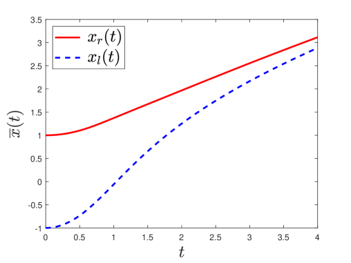
(a) Solution of (6.8)

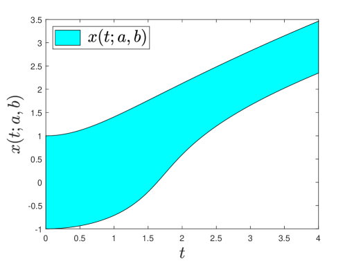
(b) Solution of (6.9)

Figure 3: Solutions of (6.8) and (6.9)

Example 6.5.

Considering the following classical differential equation with parameters

$$\begin{cases}x^{\prime}(t)=\displaystyle\frac{bt}{1+x^{2}(t)},&t\in[0,4],~b\in[1,2],\\ x(0)=a,&a\in[-1,1].\end{cases}$$ (6.9)

It is easy to see that the solution of (6.9) is

$$x(t;a,b)=y(t;a,b)-y^{-1}(t;a,b),~~~t\in[0,4],~a\in[-1,1],~b\in[1,2],$$

where

$$y(t;a,b)=\frac{1}{2}\left(6b\,t^{2}+4a^{3}+12a+2\sqrt{9b^{2}t^{4}+(12a^{3}b+36ab)t^{2}+4a^{6}+24a^{4}+36a^{2}+16}\right)^{\frac{1}{3}},$$

see Figure 3(b).

In fact, (6.9) can be regarded as the parameter differential equation of (6.8), and from Figure 3, it can be seen that the two solutions are roughly consistent. Therefore, the presented algorithm is effective.

Example 6.6.

Considering the interval differential equation

$$\begin{cases}\overline{x}^{\prime}(t)=\displaystyle\frac{[1,2]\sin t}{1+\overline{x}^{2}(t)},&t\in[0,4],\\ \overline{x}(0)=[1,3].&\end{cases}$$ (6.10)

It is easy to see that

$$\overline{x}(t)=\left[\xi(t)-\xi^{-1}(t)-\mathrm{e}^{\eta(t)-\eta^{-1}(t)},~\xi(t)-\xi^{-1}(t)+\mathrm{e}^{\eta(t)-\eta^{-1}(t)}\right],\qquad t\in[0,1],$$

where

$$\xi(t)=\frac{1}{2}\bigg(-18\cos t+74+2\sqrt{81\cos^{2}t-666\cos t+1385}\bigg)^{\frac{1}{3}},$$

$$\eta(t)=\frac{1}{2}\bigg(4\sqrt{4+9\left(\cos t-1\right)^{2}\ln^{2}2}+12\left(\cos t-1\right)\ln 2\bigg)^{\frac{1}{3}},$$

see Figure 4(a).

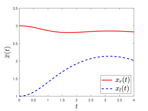
(a) Solution of (6.10)

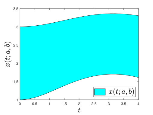
(b) Solution of (6.11)

Figure 4: Solutions of (6.10) and (6.11)

Example 6.7.

Considering the following classical differential equation with parameters

$$\begin{cases}x^{\prime}(t)=\displaystyle\frac{b\sin t}{1+x^{2}(t)},&t\in[0,4],~b\in[1,2],\\ x(0)=a,&a\in[1,3].\end{cases}$$ (6.11)

It is easy to see that

$$x(t;a,b)=y(t;a,b)-y^{-1}(t;a,b),~~~t\in[0,4],~b\in[1,2],~a\in[1,3],$$

where

$$y(t;a,b)=\frac{1}{2}\left(4a^{3}+12a+12b\left(1-\cos\!\left(t\right)\right)+4\sqrt{\left(a^{3}+3a+3b\left(1-\cos\!\left(t\right)\right)\right)^{2}+4}\right)^{\frac{1}{3}},$$

see Figure 4(b).

As showning in Figure 4, it can be seen that the two solutions of (6.10) and (6.11) are roughly consistent.

Now we present two linear interval differential equations to show the differences between the new derivative and the $gH$-derivative.

Example 6.8.

Considering the following interval differential equation

$$\begin{cases}\overline{x}^{\prime}(t)=-\overline{x}(t)+[1,2]t,&t\in[0,3],\\ \overline{x}(0)=[0,1].&\end{cases}$$ (6.12)

The corresponding parameter differential equation is given by

$$\begin{cases}x^{\prime}(t)=-x(t)+bt,&t\in[0,3],~b\in[1,2],\\ \overline{x}(0)=a,&a\in[0,1].\end{cases}$$ (6.13)

The corresponding interval differential equation under the $gH$-derivative is given by

$$\begin{cases}\overline{x}^{\prime}_{gH}(t)=-1\odot\overline{x}(t)+[1,2]\odot t,&t\in[0,3],\\ \overline{x}(0)=[0,1].&\end{cases}$$ (6.14)

The solution of (6.12) is

$$\overline{x}(t)= [x_{l}(t),x_{r}(t)]$$

$$= \left[2\mathrm{e}^{-t}+\frac{3}{2}(t-1)-\mathrm{e}^{-2\mathrm{e}^{-t}\ln 2-(t-1)\ln 2},2\mathrm{e}^{-t}+\frac{3}{2}(t-1)+\mathrm{e}^{-2\mathrm{e}^{-t}\ln 2-(t-1)\ln 2}\right],~t\in[0,3].$$

The solution of (6.13) is

$$x(t;a,b)=\mathrm{e}^{-t}\left(a+b\right)+b\left(t-1\right),~t\in[0,3],~a\in[0,1],~b\in[1,2].$$

The solutions of (6.14) are

$$\overline{x}_{1}(t) =[(x_{1})_{l}(t),(x_{1})_{r}(t)]=\left[2t-\mathrm{e}^{t}+2\mathrm{e}^{-t}-1,t+\mathrm{e}^{t}+2\mathrm{e}^{-t}-2\right],$$

$$\overline{x}_{2}(t) =[(x_{2})_{l}(t),(x_{2})_{r}(t)],$$

where

$$(x_{2})_{l}(t)=\begin{cases}2t+2\mathrm{e}^{-t}-2,&\text{ if }0\leq t\leq 1,\\ 2t-\mathrm{e}^{t-1}+2\mathrm{e}^{-t}-1,&\text{ if }1\leq t\leq 3,\end{cases}$$

$$(x_{2})_{r}(t)=\begin{cases}t+2\mathrm{e}^{-t}-1,&\text{ if }0\leq t\leq 1,\\ t+\mathrm{e}^{t-1}+2\mathrm{e}^{-t}-2,&\text{ if }1\leq t\leq 3.\end{cases}$$

From Figure 5, we can see that the solution of (6.12) is more close to that of (6.13) than that of (6.14). Moreover, as $t$ increases, the width of $\overline{x}_{1}$ and $\overline{x}_{2}$ gradually increases, and the rate of increase becomes faster and faster, which is inconsistent with the solution of (6.13).

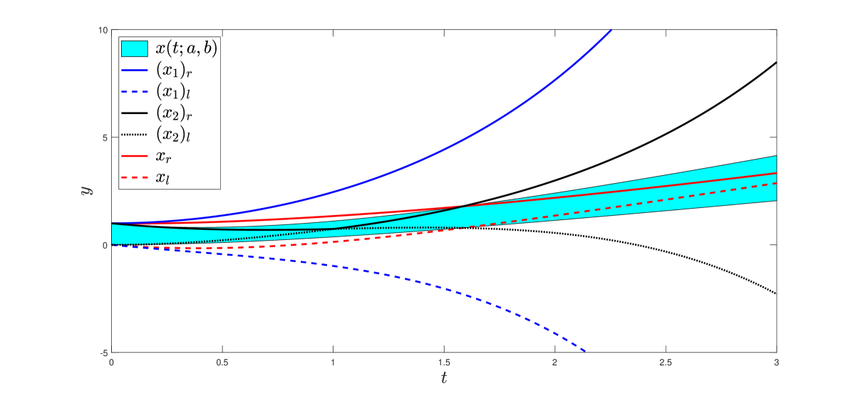
Figure 5: Solutions of (6.12)–(6.14)

Example 6.9.

Considering the interval differential equation

$$\begin{cases}\overline{x}^{\prime}(t)=\overline{x}(t)\sin t,&t\in[0,6],\\ \overline{x}(0)=[1,2].&\end{cases}$$ (6.15)

The corresponding parameter differential equation is given by

$$\begin{cases}x^{\prime}(t)=x(t)\sin t,&t\in[0,6],\\ \overline{x}(0)=a,&a\in[1,2].\end{cases}$$ (6.16)

The corresponding interval differential equation under the $gH$-derivative is given by

$$\begin{cases}\overline{x}^{\prime}_{gH}(t)=\overline{x}(t)\odot\sin t,&t\in[0,6],\\ \overline{x}(0)=[1,2].&\end{cases}$$ (6.17)

The solution of (6.15) is

$$\overline{x}(t)=[x_{l}(t),x_{r}(t)]=\left[\frac{3}{2}\mathrm{e}^{1-\cos t}-2^{-\mathrm{e}^{1-\cos t}},\frac{3}{2}\mathrm{e}^{1-\cos t}+2^{-\mathrm{e}^{1-\cos t}}\right],~t\in[0,6].$$

The solution of (6.16) is

$$x(t;a)=a\mathrm{e}^{1-\cos t},~t\in[0,6],~a\in[1,2].$$

The solutions of (6.17) are

$$\overline{x}_{1}(t) =[(x_{1})_{l}(t),(x_{1})_{r}(t)]=\left[\mathrm{e}^{1-\cos t},2\mathrm{e}^{1-\cos t}\right],$$

$$\overline{x}_{2}(t) =[(x_{2})_{l}(t),(x_{2})_{r}(t)]=\left[\frac{3}{2}\mathrm{e}^{1-\cos t}-\frac{1}{2}\mathrm{e}^{\cos t-1},\frac{3}{2}\mathrm{e}^{1-\cos t}+\frac{1}{2}\mathrm{e}^{\cos t-1}\right],$$

$$\overline{x}_{3}(t) =[(x_{3})_{l}(t),(x_{3})_{r}(t)],$$

$$\overline{x}_{4}(t) =[(x_{4})_{l}(t),(x_{4})_{r}(t)],$$

where

$$(x_{3})_{l}(t)=\begin{cases}\mathrm{e}^{1-\cos t},&t\in[0,\pi],\\ \frac{3}{2}\mathrm{e}^{1-\cos t}-\frac{1}{2}\mathrm{e}^{3+\cos t},&t\in[\pi,6],\\ \end{cases}$$

$$(x_{3})_{r}(t)=\begin{cases}2\mathrm{e}^{1-\cos t},&t\in[0,\pi],\\ \frac{3}{2}\mathrm{e}^{1-\cos t}+\frac{1}{2}\mathrm{e}^{3+\cos t},&t\in[\pi,6],\\ \end{cases}$$

$$(x_{4})_{l}(t)=\begin{cases}\frac{3}{2}\mathrm{e}^{1-\cos t}-\frac{1}{2}\mathrm{e}^{-1+\cos t},&t\in[0,\pi],\\ \frac{3}{2}\mathrm{e}^{1-\cos t}-\frac{1}{2}\mathrm{e}^{-3-\cos t},&t\in[\pi,6],\\ \end{cases}$$

$$(x_{4})_{r}(t)=\begin{cases}\frac{3}{2}\mathrm{e}^{1-\cos t}+\frac{1}{2}\mathrm{e}^{-1+\cos t},&t\in[0,\pi],\\ \frac{3}{2}\mathrm{e}^{1-\cos t}+\frac{1}{2}\mathrm{e}^{-3-\cos t},&t\in[\pi,6].\\ \end{cases}$$

From Figure 6, we can see that the solution $\overline{x}_{3}$ has the width issue; the latter half of $\overline{x}_{4}$ almost overlaps; $\overline{x}_{2}$ and $\overline{x}$ are almost identical, only $\overline{x}_{1}$ perfectly coincides with the solution $x(t,a,b)$. However, due to the issue of switching points, as $t$ increases, the number of solutions to (6.14) will doubly increase, which makes solving the equation complicated.

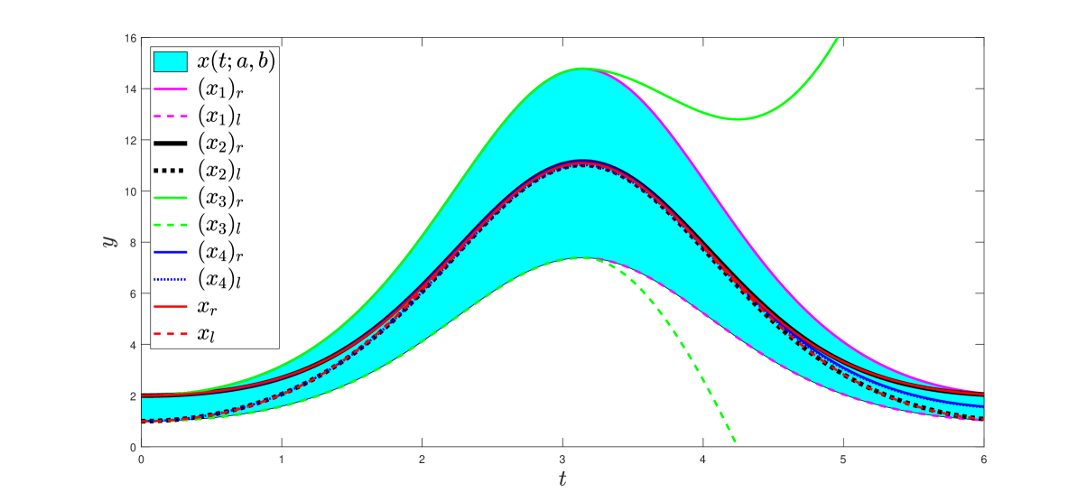
Figure 6: Solutions of (6.15)–(6.17)

7 Conclusion

In this paper, we jump out of the original framework of interval arithmetic operations, and present new ones. With the proposed arithmetic operations, the space $\mathbb{R}_{\mathcal{I}}$ is a linear space, while it is a semilinear space with traditional operations. Moreover, new distance, norm, and inner product are presented to show that $\mathbb{R}_{\mathcal{I}}$ is a Hilbert space. On this basis, novel definitions of derivative and integral for interval-valued functions are introduced, and their fundamental properties are systematically investigated. The proposed approach is particularly interesting due to its computational simplicity compared to existing methods. These new definitions simultaneously incorporate aspects of both the classical and multiplicative derivatives and integrals, offering a hybrid framework that retains the strengths of each. This dual-structure method not only simplifies calculations but also enhances the interpretability and applicability of the interval analysis. The classical derivative and integral are widely used in various applications. In contrast, the multiplicative derivative and integral are especially effective for modeling processes characterized by proportional or exponential growth, offering new perspectives in the analysis of interval-valued functions. Therefore, the physical interpretation of the newly introduced concepts of derivative and integral becomes more transparent and meaningful within this unified framework.

In the future, these results could be wildly applied in other mathematical branches, such as interval integration inequalities, interval differential equations, interval optimization, interval decision making and so on. Also, it is easy to extend the new framework to fuzzy numbers, and the calculus of fuzzy-valued functions. These could be of interest in many fields, such as finance, economics, environment, and engineering.

Funding

This paper was supported by “the Fundamental Research Funds for the Central Universities” (No. B250201169).

Declaration of interests

The authors declare that they have no known competing financial interests or personal relationships that could have appeared to influence the work reported in this paper.