Holographically Emergent Gauge Theory in Symmetric Quantum Circuits

Abstract

We develop a novel holographic framework for mixed-state phases in random quantum circuits, both unitary and non-unitary, with a global symmetry $G$. Viewing the circuit as a tensor network, we decompose it into two parts: a symmetric layer, which defines an emergent gauge wavefunction in one higher dimension, and a random non-symmetric layer, which consists of random multiplicity tensors. For unitarity circuits, the bulk gauge state is deconfined, but under a generic non-unitary circuit (e.g. channels), the bulk gauge theory can undergo a decoherence-induced phase transition: for $G\,{=}\,\mathbb{Z}_{N}$ with local symmetric noise, the circuit can act as a quantum error-correcting code with a distinguished logical subspace inheriting the $\mathbb{Z}_{N}$-surface code’s topological protection. We then identify that the charge sharpening transition from the measurement side is complementary to a decodability transition in the bulk: noise of the bulk can be interpreted as measurement from the environment. For $N\,{\leq}\,4$, weak measurements drive a single transition from a charge-fuzzy phase with sharpening time $t_{\#}\sim e^{L}$ to a charge-sharp phase with $t_{\#}\sim\mathcal{O}(1)$, corresponding to confinement that destroys logical information. For $N>4$, measurements generically generate an intermediate quasi-long-range ordered Coulomb phase with gapless photons and purification time $t_{\#}\sim\mathcal{O}(L)$.

I Introduction

Measurement-induced phase transitions (MIPTs) are now recognized as universal phenomena which appear in open quantum systems undergoing local scrambling and measurement dynamics [1, 2, 3, 4, 5, 6, 7, 8, 9, 10, 11, 12, 13, 14, 15, 16, 17]. As the measurement rate $p$ is increased past a critical value $p_{c}$, the steady-state entanglement entropy of subregions exhibits a sharp transition from a volume law to an area law. Equivalently, MIPTs can be viewed as purification transitions: once $p>p_{c}$, an initially mixed state purifies on a timescale $t_{p}\sim\mathcal{O}(1)$ that is independent of system size [9]. They may also be interpreted as error-correction transitions, in which sufficiently frequent measurements overwhelm the scrambling dynamics and prevent quantum information from being hidden from the measuring observer [9, 10].

Incorporating symmetries into the dynamics enriches the phase diagram and qualitatively modifies operator spreading and entanglement growth [18, 19, 20, 21, 22]. In 1D random unitary circuits with local measurements and a global U(1) symmetry, the volume-law phase splits into two phases, charge sharp and charge fuzzy, separated by a second critical measurement rate $p_{\#}<p_{c}$ [23, 24, 25, 26, 27, 25, 28, 29, 30, 31]. This charge-sharpening transition is characterized by the timescale $t_{\#}$ needed to infer the global charge from local measurement records: for $p<p_{\#}$, $t_{\#}\sim L$, while for $p>p_{\#}$, $t_{\#}\sim\mathcal{O}(1)$, even though identifying the microscopic state still requires exponentially long times.

Measurements introduce intrinsic stochasticity into the dynamics, with each sequence of outcomes generating a distinct final state or “trajectory”. Each trajectory occurs with a probability determined by the Born rule. Measurement-induced phase transitions arise from qualitative changes in the ensemble of such trajectories; they are mixed-state phase transitions. Other prominent examples of mixed-state transitions include decoherence-induced phase transitions in topological error-correcting codes [32, 33, 34, 35, 36, 37, 38, 39, 40]. Developing a complete classification of mixed-state orders in open quantum systems remains a central challenge, although significant progress has been made in this direction in recent years.

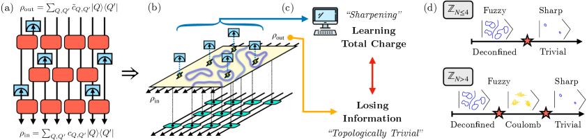
Figure 1: Summary. (a) Monitored Symmetric Circuit. The circuit consists of two parts: local symmetric gates and local charge measurements. One can map a symmetric monitored random circuit into the tensor network. (b) Two-layer tensor network. The top layer of the model is constructed using the Clebsch-Gordon coefficients of the group and realizes a gauge theory. The bottom layer is comprised of random multiplicity tensors. (c) Sharpening transition. Charge sharpening occurs when local charge measurements extract the global charge of the spin chain. At the same time, information encoded in the gauge wavefunction is destroyed. Therefore, fuzzy (sharp) phase corresponds to information protected (lost) in the gauge theory. (d) Phase diagram. For $\mathbb{Z}_{N<4}$, there exists only two phases: truly fuzzy (deconfined) and sharp (trivial), where sharpening time scales as $\exp(L)$ and ${\cal O}(1)$, respectively. However, for $\mathbb{Z}_{N\geq 4}$ an intermediate Coulomb (QLRO) phase opens up, where the purification time scales as ${\cal O}(L)$. In the limit $N\rightarrow\infty$, where the symmetry becomes U(1), the deconfined phase collapses into a point.

Here we propose a novel framework to understand the mixed state phases arising in random symmetric circuits through the lens of a holographically emergent gauge theory. This framework is general, enabling the study of such mixed state transitions in circuits with arbitrary abelian or non-abelian symmetries. Leveraging powerful tensor network techniques [41, 42, 43, 44], we decompose symmetric random circuits into a two-layered tensor network: a symmetric layer describing propagation of charged degrees of freedom and a non-symmetric layer describing propagation of uncharged ones (see  Fig. 1). We show that for a $1$ dimensional quantum system endowed with a global $G$-symmetry, this symmetric layer constitutes a $2$ dimensional $G$-gauge wavefunction (or more generally a $G$-spin network state [45, 46, 47]). Controlled calculations are possible when the uncharged layer has a large bond dimension. This condition confines us to the volume-law phase, where the $(S_{n}\times S_{n})\rtimes\mathbb{Z}_{2}^{\mathbb{H}}$ replica symmetry is spontaneously broken. Note that this is precisely the regime where a charge sharpening transition occurs.

For random unitary circuits endowed with a $G$-symmetry, we show that averaging over the non-symmetric layer generically produces a gauge state with long range entanglement (LRE)-a coherent superposition of all allowed string-net configurations. When $G=\mathbb{Z}_{N}$, we obtain precisely the deconfined fixed point state of $\mathbb{Z}_{N}$ gauge theory. In this case, the global symmetry operator of the spin chain maps to a non-contractible ’t Hooft loop in the emergent gauge theory. Thus, different global charge sectors of the spin chain correspond to distinct topological sectors of the gauge theory.

We further extend the bulk-boundary correspondence to the case of spin chains evolving under symmetric gates and subject to local noise channels that act only on the charge degrees of freedom at each timestep. In this setting, the emergent bulk gauge theory realizes a dynamically generated topological code, with the same noise channel applied to every link of the code. When $G=\mathbb{Z}_{N}$, we obtain precisely the $\mathbb{Z}_{N}$ surface code [48, 49]. This observation naturally identifies a set of logical states for the $\mathbb{Z}_{N}$ symmetric spin chain, one within each global charge sector. Logical information encoded in this basis inherits the topological protection of the bulk surface code, and therefore remains robust against sufficiently weak noise. We make this correspondence precise by showing that the coherent information of the spin chain evolving under the noisy channel, after averaging over the uncharged layer, is exactly equal to the coherent information of the noisy bulk topological code. This establishes a sharp equivalence between the mixed-state phase diagram of the random symmetric quantum circuit in its volume-law phase and the mixed-state phase diagram of a noisy topological code.

Finally, we turn to the specific example of charge-sharpening transitions in monitored circuits. We consider $\mathbb{Z}_{N}$ symmetric circuits subject to weak (imperfect) charge measurements on every spin at each timestep. In the bulk description, this procedure produces a gauge theory state subjected to weak measurements on every link. Charge sharpening occurs when measurements collapse an initial coherent superposition of several global charge sectors onto a single, definite sector. Within the bulk description, this precisely corresponds to a decodability transition whereby logical information encoded in the surface code is destroyed. Furthermore, we show that this phenomenon admits a natural interpretation as a confinement transition [50, 51]. While our framework applies to general symmetry groups, we present explicit calculations for $\mathbb{Z}_{N}$ symmetric circuits. In the charge-fuzzy phase, the post-measurement ensemble of gauge wavefunctions retains long-range entanglement (LRE) leading to an exponentially large sharpening timescale $(t_{\#}\sim e^{L})$. Once the system crosses the sharpening threshold, the ensemble supports only short-range entanglement (SRE), resulting in a rapid sharpening timescale $(t_{\#}\sim\mathcal{O}(1))$. We show that when $N>4$, the bulk gauge theory can enter an intermediate Coulombic phase featuring emergent gapless photons and power-law correlations. In this regime the sharpening timescale becomes linear, $(t_{\#}\sim L)$, mirroring the behavior found in the $U(1)$ symmetric circuits. New phases emerging from non-abelian symmetric circuits will be discussed in a forthcoming work.

II Emergent Gauge State from random symmetric circuits

In this section, we show how a gauge-theory wavefunction naturally emerges from random quantum circuits with on-site global symmetry $G$ [44, 41, 42, 43, 52].

We consider a spin chain of length $L$, with local Hilbert space $\mathcal{H}$ of dimension $q$. The global Hilbert space is $\mathcal{H}_{\text{global}}=\mathcal{H}^{\otimes L}$, with total dimension $q^{L}$. Starting from an initial state $\ket{\psi_{0}}\in\mathcal{H}_{\text{global}}$, we evolve with a (possibly non-unitary) brickwork circuit operator $\mathcal{U}_{\text{circuit}}$ built from local gates that act on nearest neighbors, see Fig. 2.

We can transform a local gate $U$ acting on $k$-sites to a (vertex) state by writing its singular value decomposition and vectorizing it [53, 54]:

$$U=\sum_{i}\lambda_{i}\ket{l_{i}}\bra{r_{i}}\rightarrow\ket{U}=\sum_{i}\lambda_{i}\ket{l_{i}}\ket{r^{*}_{i}}$$ (1)

As a $k$-local operator, $U:\mathcal{H}^{\otimes k}\rightarrow\mathcal{H}^{\otimes k}$ and $\ket{U}\in\mathcal{H}^{\otimes k}\otimes\mathcal{H}^{*\otimes k}$. The vertex states are connected to one another by projecting them along maximally entangled EPR pairs, $\ket{I}=\sum_{i}\ket{i}\ket{i^{*}}$, which correspond to the vectorization of the identity operator. With such a definition, the final output of the circuit can be formally written as

$$|\Psi_{\textrm{out}}\rangle=\Big[\langle\Psi_{\textrm{in}}|\otimes\langle\bm{I}|\Big]\cdot|\bm{U}\rangle,$$ (2)

where $|\bm{U}\rangle:=\otimes_{v}|U_{v}\rangle$ is the tensor product of all gate states, $|\bm{I}\rangle:=\otimes_{l}|I_{l}\rangle$ is the tensor product of all link EPR pairs, and $|\Psi_{\rm in}\rangle$ is the input state.

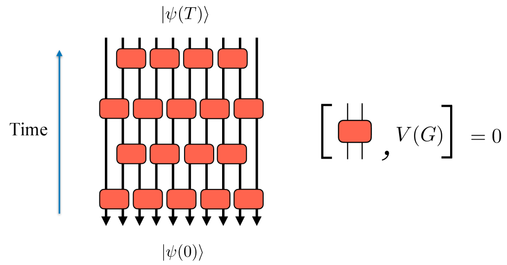
Figure 2: Random Symmetric Circuits: We consider a random symmetric circuit with bricklayer geometry as depicted. The symmetry group $G$ acts by means of some unitary representation $V(\cdot):G\rightarrow\mathcal{U}(\mathcal{H}_{\text{global}})$. Each gate is individually chosen to commute with the group action but are otherwise random.

II.1 Charge Basis

The on-site symmetry is implemented by a unitary representation $V(\cdot):G\rightarrow\mathcal{U}(\mathcal{H}_{\text{global}})$ acting locally on the spin chain as $V(g)=\bigotimes_{i=1}^{L}V_{i}(g)$. Then, symmetry of the circuit is imposed by requiring

$$[U,V(g)]=0,$$ (3)

Since any finite-dimensional representation decomposes into the sum of irreducible representations (irreps), the local Hilbert space can be written as

$$\mathcal{H}=\bigoplus_{j}n_{j}\mathcal{R}_{j}$$ (4)

where $\mathcal{R}_{j}$ is a $G$-irrep labeled by $j$ and $n_{j}$ is its multiplicity. Therefore, we choose the following local basis

$$\ket{j,\mu_{j},a_{j}}$$ (5)

where $j$ labels the irrep, $\mu_{j}$ denotes a state within the irrep $j$, and $a_{j}$ is a multiplicity index associated with that irrep. Whenever possible, we omit the subscripts on $\mu_{j}$ and $a_{j}$ to simplify the notation. The symmetry operators $V(g)$ are block-diagonal in the irrep labels and act trivially on the multiplicity spaces:

$$V(g)=\bigoplus_{j}V^{j}(g)\otimes\mathbb{I}_{n_{j}},$$ (6)

where $\mathbb{I}_{n{j}}$ is the identity operator on the $n_{j}$-dimensional multiplicity space for the irrep labeled by $j$.

II.2 Symmetry Decomposition of Vertex Tensors

The symmetry of a local gate implies that its vectorized state $\ket{U}$ must be a group singlet under the action of $G$. If $V(g)$ acts on the “ket” legs and $V(g)^{*}$ on the “bra” legs, we have

$$\ket{U}=V(g)\otimes V(g)^{*}\ket{U},$$ (7)

for all $g\in G$. It is convenient to encode whether a leg is incoming or outgoing by an arrow on each link: when the arrow points into a vertex, we conjugate the irrep label on that leg; when it points out, we do not.

We expand $\ket{U}$ in the basis Eq. (5). Introducing a joint index $J=(j,\mu_{j},a_{j})$ and $\mathbf{J}=(J_{1},\dots,J_{2k})$, we write

$$\ket{U}=\sum_{\mathbf{J}}A^{\mathbf{J}}\otimes_{i=1}^{2k}\ket{J_{i}},$$ (8)

where $A^{\mathbf{J}}$ is a tensor with one index per leg. Symmetry implies that $A^{\mathbf{J}}$ is an invariant tensor of $G$ [44, 41, 42, 43].

Representation theory then constrains the structure of such tensors. As a warm-up, consider a two-legged tensor $A^{J_{1}J_{2}}$ with one incoming and one outgoing leg. The invariance condition reads

$$A^{J_{1}J_{2}}=\sum_{J_{1}^{\prime},J_{2}^{\prime}}V^{J_{1}J_{1}^{\prime}}(g)A^{J_{1}^{\prime}J_{2}^{\prime}}[V^{J_{2}^{\prime}J_{2}}(g)]^{\dagger},$$ (9)

for all $g\in G$. By Schur’s lemma, such an invariant tensor must be proportional to the identity within each irrep block:

$$A^{J_{1}J_{2}}=\delta^{j_{1}j_{2}}\delta_{\mu_{1}\mu_{2}}T^{j_{1}j_{2}}_{a_{1}a_{2}},$$ (10)

where $T^{j_{1}j_{2}}_{a_{1}a_{2}}$ is an unconstrained multiplicity tensor. The generalization to both legs incoming or both outgoing is obtained by conjugating the corresponding irrep labels.

The first nontrivial case is a three-legged tensor $A^{J_{1}J_{2}J_{3}}$ with, say, two incoming and one outgoing leg. The irreps obey a fusion algebra

$$\mathcal{R}_{i}\otimes\mathcal{R}_{j}=\bigoplus_{k}N^{k}_{ij}\mathcal{R}_{k}$$ (11)

where $N_{ij}^{k}$ is the multiplicity of the channel $i\times j\to k$. For notational simplicity, assume the group is multiplicity-free in fusion, $N_{ij}^{k}\leq 1$. The Clebsch-Gordan coefficients

$$C^{j_{1}j_{2}j_{3}}_{\mu_{1}\mu_{2}\mu_{3}}=\innerproduct{j_{3},\mu_{3}}{j_{1},\mu_{1};j_{2},\mu_{2}}$$ (12)

are invariant tensors of the group . By the Wigner-Eckart theorem, any three-legged invariant tensor can be decomposed as

$$A^{J_{1}J_{2}J_{3}}=C^{j_{1}j_{2}j_{3}}_{\mu_{1}\mu_{2}\mu_{3}}T^{j_{1}j_{2}j_{3}}_{a_{1}a_{2}a_{3}},$$ (13)

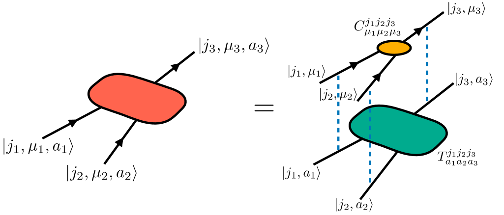
Figure 3: Symmetry Decomposition I. Here we depict the symmetry decomposition of a trivalent vertex with two incoming legs and one outgoing leg.

where $T^{j_{1}j_{2}j_{3}}_{a_{1}a_{2}a_{3}}$ is an unconstrained multiplicity tensor. In other words, symmetry splits the tensor into a fixed charged part $C$ (the intertwiner) and a free multiplicity part $T$, see Fig. 3. A similar structure holds for four-legged tensors. Consider a tensor $A^{J_{1}J_{2}J_{3}J_{4}}$ with two outgoing legs labeled by $j_{1},j_{2}$ and two incoming legs labeled by $j_{3},j_{4}$. Suppose $j_{1}\otimes j_{2}$ and $j_{3}\otimes j_{4}$ both contain an intermediate irrep $e$. Then an invariant tensor can be built as

$$B^{j_{1}j_{2},j_{3},j_{4};e}_{\mu_{1}\mu_{2}\mu_{3}\mu_{4}}=\sum_{\mu_{e}}\big(C^{j_{1}j_{2}e}_{\mu_{1}\mu_{2}\mu_{e}}\big)^{*}C^{j_{3}j_{4}e}_{\mu_{3}\mu_{4}\mu_{e}}.$$ (14)

whose structure is again fixed by the symmetry group $G$. There is one such invariant tensor for each allowed intermediate charge $e$. A generic four-legged invariant tensor then decomposes as

$$A^{J_{1}J_{2}J_{3}J_{4}}=\sum_{e}B^{j_{1}j_{2},j_{3},j_{4};e}_{\mu_{1}\mu_{2}\mu_{3}\mu_{4}}T^{j_{1}j_{2}j_{3}j_{4};e}_{a_{1}a_{2}a_{3}a_{4}},$$ (15)

where $T^{j_{1}j_{2}j_{3}j_{4};e}_{a_{1}a_{2}a_{3}a_{4}}$ is again an unconstrained multiplicity tensor, see Fig. 4. In fact, we can interpret Eq. (14) as a way to split the four-legged vertex into a pair of three-legged vertices connected by an internal link which itself carries charge and state labels. The result of this splitting is to transform the square lattice of the charged layer into a hexagonal lattice with Clebsch-Gordon tensors sitting at each trivalent vertex (Fig. 6).

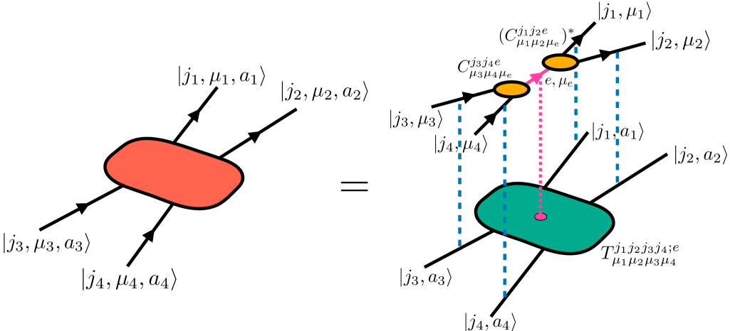
Figure 4: Symmetry Decomposition II. Here we depict the symmetry decomposition of a four-legged vertex with two incoming legs and two outgoing legs.

Different ways of associating a four-legged tensor to trivalent fusion trees are related by $F$-moves. For example, an alternative fusion channel built from

$$\tilde{B}^{j_{1}j_{2},j_{3},j_{4};f}_{\mu_{1}\mu_{2}\mu_{3}\mu_{4}}=\sum_{\mu_{f}}C^{j_{3}fj_{1}}_{\mu_{3}\mu_{f}\mu_{1}}C^{j_{2}^{*}j_{4}f}_{\mu_{2}\mu_{4}\mu_{f}}$$ (16)

is related to the previous one by

$$B^{j_{1}j_{2},j_{3},j_{4};e}=\sum_{f}F^{j_{1}j_{2}e}_{j_{3}j_{4}f}\tilde{B}^{j_{1}j_{2},j_{3},j_{4};f},$$ (17)

where $F$ is the F-symbol of the underlying unitary fusion category, see Fig. 5. These F-symbols obey the pentagon equation [56]. The resulting structure is that of a unitary modular tensor category, familiar from the description of bosonic topologically ordered phases.

For tensors with more legs, one iteratively decomposes into trivalent intertwiners, summing over internal charges on intermediate links. Different trivalent graphs are related by sequences of $F$-moves. We refer to this insensitivity to the underlying trivalent graph as background independence [52].

The Abelian case is particularly simple. Fusion of irreps produces a single irrep, and all irreps are one dimensional. The Clebsch-Gordan tensors reduce to Kronecker delta functions enforcing charge conservation. The symmetry constraint for a $2k$-legged tensor then takes the form

$$A^{J_{1},\dots,J_{2k}}=B^{j_{1},\dots,j_{2k}}T^{j_{1},\dots,j_{2k}}_{a_{1},\dots,a_{2k}},$$ (18)

where $B^{j_{1},\dots,j_{2k}}=1$ if the Abelian charge-selection rule is satisfied at the vertex and zero otherwise. There is no need to explicitly decompose into trivalent tensors in this case.

Collecting these observations, each symmetric vertex tensor can be written as a product

$$A^{\mathbf{J}}=B^{\mathbf{j};\mathbf{e}}_{\bm{\mu}}T^{\mathbf{j};\mathbf{e}}_{\bm{a}},$$ (19)

where $B$ encodes the Clebsch-Gordan data and intermediate charges $\mathbf{e}$, and $T$ is an unconstrained multiplicity tensor. We refer to $B$ as the charged tensor and $T$ as the multiplicity tensor. Finally, the full tensor network is obtained by contracting vertex states $\ket{U}$ with EPR pairs. In the symmetry basis, each EPR pair takes the form $\ket{I}=\sum_{j,\mu,a}\ket{j,\mu,a}\ket{j^{*},\mu,a}$.

II.3 Constructing the Gauge Wavefunction

We now show that the charged layer, obtained by contracting Clebsch-Gordan tensors across the circuit, defines a gauge-theory wavefunction $\ket{\Phi_{\text{g}}}$. For concreteness, we assume that the charged layer has been decomposed into a trivalent graph, with a Clebsch-Gordan tensor $C_{v}$ assigned to each vertex $v$.

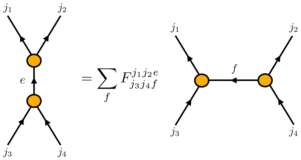
Figure 5: $F$-move. Local move relating different trivalent decompositions of a four-legged invariant tensor via F-symbols.

Fix an assignment of irrep labels $\mathbf{j}=\{j_{l}\}$ on the links of this graph. Contractions of $\bm{\mu}$-indices between neighboring intertwiners are nonzero only if the irrep labels on the two ends of each oriented link are conjugate to one another; equivalently, we may treat each link as carrying a single charge label $j_{l}$. Tracing over the internal state labels $\bm{\mu}$, we obtain a wavefunction on configurations of link charges. Explicitly, we define

$$\ket{\Phi_{\text{g}}}=\sum_{\{j_{l}\}}\operatorname{Tr}_{\bm{\mu}}\bigg[\prod_{v}(C_{v})^{j_{1}j_{2}j_{3}}_{\mu_{1}\mu_{2}\mu_{3}}\bigg]\bigotimes_{l}\ket{j_{l}},$$ (20)

where the trace contracts $\bm{\mu}$ indices on neighboring tensors, and the product runs over vertices of the trivalent graph. In analogy with PEPS, the link charges $j_{l}$ play the role of “physical” degrees of freedom, while the $\mu$-indices are virtual.

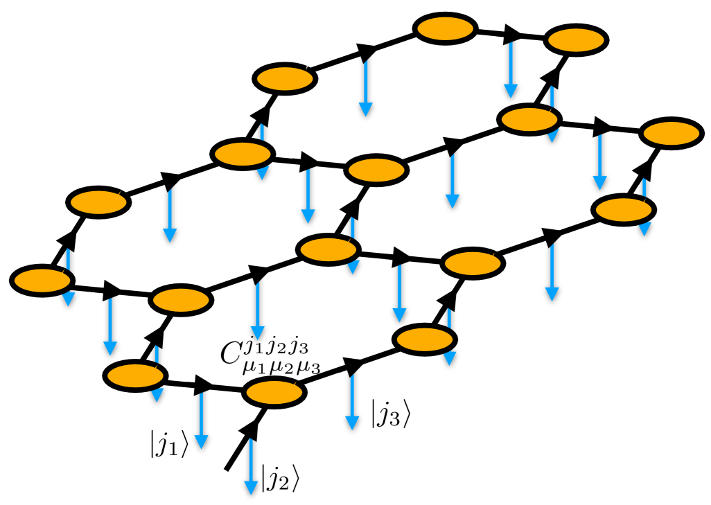
Figure 6: Gauge wavefunction in the charged layer. Decomposing four-legged symmetric vertices into trivalent Clebsch-Gordan tensors transforms the square lattice into a hexagonal lattice with trivalent vertices. Link degrees of freedom carry irrep labels $j_{l}$, while internal indices $\mu$ are summed over. Clebsch-Gordan tensors act as intertwiners enforcing gauge-invariant flux configurations.

To further proceed, on each link we interpret the charge (irreps) as an electric flux (string labels) in the corresponding lattice gauge theory:

$$\text{Charges on links}\longleftrightarrow\text{electric fluxes}.$$ (21)

The Clebsch-Gordan tensors $C_{v}$ specify the allowed fusion channels of flux lines meeting at each vertex, see Fig. 6. Furthermore, the fact that each $C_{v}$ should be a group singlet implies an exact lattice Gauss law. At a vertex $v$, define the gauge transformation operator

$$\mathcal{G}_{v}(g)=\prod_{l\in v}V^{j_{l}}(g),$$ (22)

where the product runs over links $l$ incident on $v$, and $V^{j_{l}}(g)$ acts in irrep $j_{l}$. When a link is oriented towards $v$, we act with the conjugate representation; when it is oriented away from $v$, we act with the original representation. Under $\mathcal{G}_{v}(g)$, the Clebsch-Gordan tensor at $v$ transforms as

$$(C_{v})^{\cdots j_{l}\cdots}_{\cdots\mu_{l}\cdots}\rightarrow\sum_{\nu_{l}}V^{j_{l}}(g)_{\mu_{l}\nu_{l}}(C_{v})^{\cdots j_{l}\cdots}_{\cdots\nu_{l}\cdots}.$$ (23)

Since $C_{v}$ is an invariant tensor, these transformations cancel around each vertex, and the full state obeys

$$\mathcal{G}_{v}(g)\ket{\Phi_{\text{g}}}=\ket{\Phi_{\text{g}}},$$ (24)

for all vertices $v$ and all $g\in G$. Thus $\ket{\Phi_{\text{g}}}$ is a pure-gauge state with no static charges.

Finally, the geometry of the original circuit induces boundary conditions for $\ket{\Phi_{\text{g}}}$. Initial and final time slices correspond to rough boundaries, which can be viewed as sourcing edge charges and the associated flux lines. The left and right spatial boundaries are smooth, where electric strings can terminate without exposing unscreened charge. In a deconfined phase, flux lines can spread through the bulk, while in a confining phase the amplitude for long electric strings decays as $e^{-T_{\text{str}}l}$, suppressing flux penetration into the circuit bulk (an “electric Meissner” effect).

II.4 Bulk-Boundary Correspondence

The two-layer structure of the symmetric tensor network can now be made explicit: the full network is a contraction of multiplicity tensors on top of a fixed bulk spin-network state encoding the charged degrees of freedom [57, 44], see Fig. 7. At each spacetime vertex $v$, we define the multiplicity vertex state

$$\ket{T_{v}}=\sum_{\bm{j},\bm{a}}(T_{v})^{\bm{j}}_{\bm{a}}\bigotimes_{i=1}^{2k}\ket{j_{i},a_{i}},$$ (25)

where the product runs over the legs attached to $v$. The bulk charged state $\ket{\Phi_{\text{g}}}$ lives on link degrees of freedom.

To glue these link variables to vertex multiplicity variables, we introduce an isometry $E$ that embeds the link Hilbert space into an extended Hilbert space with one copy of $(j,a)$ at each end of the link. For an oriented link $l:x\to y$, we define

$$E_{l}:\ket{j}\mapsto\frac{1}{\sqrt{n_{j}}}\sum_{a}\ket{j^{*},a}_{xy}\otimes\ket{j,a}_{yx},$$ (26)

where the charge at the beginning of the link is conjugated and the charge at the end is not. On links internal to the trivalent decomposition (which are not present in the original circuit), we let $E_{l}$ act as the identity. The full isometry is the product over all physical links,

$$E=\prod_{\text{links }l}E_{l},\quad E^{\dagger}E=\mathbb{I}.$$ (27)

In gauge-theory language, $E$ is the canonical embedding into the extended Hilbert space [58, 59].

Finally, contracting the gauge wavefunciton $|\Phi_{g}\rangle$ with the embedding tensor $E$, and then with the multiplicity tensor yields a boundary state on the initial and final time slices (c.f. Eq. (2)):

$$\ket{\Phi_{\text{Bdy}}}=\Big(\hskip-2.0pt\otimes_{v}\hskip-2.0pt\langle T_{v}|\Big)E\ket{\Phi_{\text{g}}}.$$ (28)

Further contracted with a fixed initial state $|\Psi_{\textrm{in}}\rangle$, Eq. (28) expresses the final state of the spin chain in terms of the bulk gauge wavefunction and the random multiplicity tensors. This realizes a discrete bulk-boundary correspondence: the global symmetry of the boundary state arises as the remnant of bulk gauge invariance, with the bulk direction identified with time.

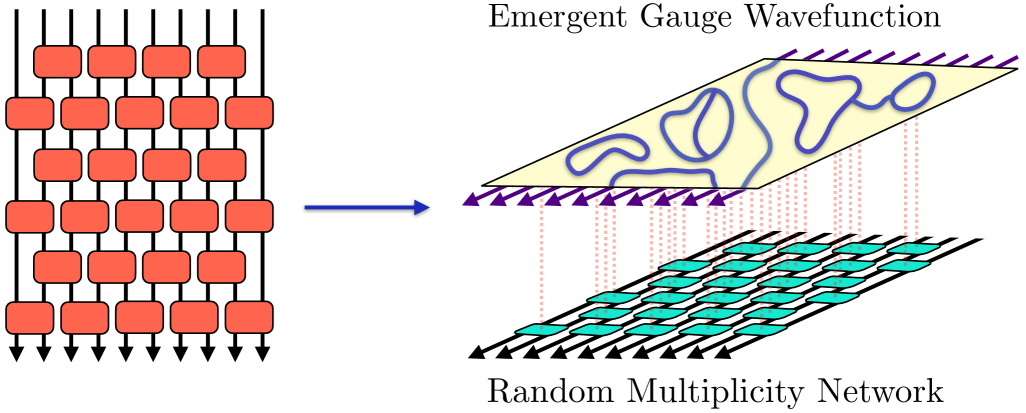
Figure 7: Bulk-boundary correspondence. The symmetric circuit tensor network factorizes into a fixed charged (bulk) layer and a random multiplicity (boundary) layer. Contracting the bulk spin network with random multiplicity tensors produces the boundary state.

We can generalize this construction to circuits with additional symmetric noise or measurements. Consider a brickwork circuit of $G$-symmetric gates, followed after each layer by a local quantum channel $\mathcal{E}^{t}$ that factorizes over sites,

$$\mathcal{E}^{t}(\cdot)=\prod_{k=1}^{L}\mathcal{E}^{t}_{k}(\cdot),$$ (29)

with each $\mathcal{E}^{t}_{k}$ admitting a Kraus representation

$$\mathcal{E}(\cdot)=\sum_{\alpha}p_{\alpha}K_{\alpha}(\cdot)K_{\alpha}^{\dagger}.$$ (30)

We assume that the Kraus operators commute with the symmetry,

$$[K_{\alpha},V(g)]=0,$$ (31)

and act diagonally on multiplicity indices, so that they modify only the charged degrees of freedom. Examples include local charge-measurement channels.

In this setting, the bulk charged state $\ket{\Phi_{\text{g}}}$ is replaced by a mixed state

$$\rho_{\text{g}}=\prod_{\mu}\mathcal{E}_{\mu}\big(\ket{\Phi_{\text{g}}}\bra{\Phi_{\text{g}}}\big),$$ (32)

where the product runs over links $\mu$ of the gauge lattice and $\mathcal{E}_{\mu}$ acts on the corresponding charged degree of freedom. The bulk-boundary correspondence becomes

$$\rho_{\text{Bdy}}=\Big(\bigotimes_{v}\bra{T_{v}}\Big)E\rho_{\text{g}}E^{\dagger}\Big(\bigotimes_{v}\ket{T_{v}}\Big).$$ (33)

Thus, local symmetric channels acting on the spin chain map to local operations on the bulk gauge wavefunction, while the multiplicity layer still provides a random projection from bulk to boundary.

II.5 Unitarity and Deconfinement

So far, we have not imposed any requirement on the local gates other than symmetry. We now restrict our attention to $2\times 2$ unitary gates and examine what unitarity imposes on the structure of the gauge wavefunction. We first focus on the case where $G$ is abelian. In this setting, $\mu_{j}$ label is trivial, and there is no fusion multiplicity. Since all intermediate charge sectors are fixed, we may simply write

$$A^{j}_{\bm{a}}=B^{\bm{j}}T^{\bm{j}}_{\bm{a}}.$$ (34)

The $B^{\bm{j}}$ tensor is 1 if the charges obey the appropriate selection rule and is 0 otherwise. Any constant prefactor can be re-absorbed into $T^{\bm{j}}_{\bm{a}}$.

II.5.1 $G=\mathbb{Z}_{N}$

We first consider $\mathbb{Z}_{N}$-symmetric circuits with $D$-dimensional local Hilbert space, $\mathcal{H}=\bigotimes_{j=0}^{N-1}nR_{j}$. Here each one-dimensional irrep $R_{j}$ appears with multiplicity $n$. Separating the charge labels $\bm{j}$ into incoming and outgoing parts, $\bm{j}_{\text{in}}$ and $\bm{j}_{\text{out}}$, the $\mathbb{Z}_{N}$ charge conservation rule can be written as

$$\sum_{i}j_{\text{in},i}=\sum_{i}j_{\text{out},i}\pmod{N}.$$ (35)

Defining the total incoming and outgoing charges as $J_{\text{in}}=\sum_{i}j_{\text{in},i}$ and $J_{\text{out}}=\sum_{i}j_{\text{out},i}$ respectively allows us to express the matrix elements of the gate in the form

$$A^{\bm{j}_{\text{out}}\bm{j}_{\text{in}}}_{\bm{a}_{\text{out}}\bm{a}_{\text{in}}}=\delta^{J_{\text{out}},J_{\text{in}}}T^{\bm{j}_{\text{out}}\bm{j}_{\text{in}}}_{\bm{a}_{\text{out}}\bm{a}_{\text{in}}}$$ (36)

Thus, the gate is block-diagonal in total charge sectors, labeled by $J=J_{\text{out}}=J_{\text{in}}$. The total charge $J$ takes values $0,1,\dots,N-1$, giving rise to $N$ independent charge sectors. Each block $T^{J}$ acts within a subspace of dimension $D=Nn^{2}$. For instance, for $\mathbb{Z}_{3}$, $U$ would look like

$$U=\begin{bmatrix}\framebox{$T^{0}_{3n^{2}\crossproduct 3n^{2}}$}&0&0\\ 0&\framebox{$T^{1}_{3n^{2}\crossproduct 3n^{2}}$}&0\\ 0&0&\framebox{$T^{2}_{3n^{2}\crossproduct 3n^{2}}$}\\ \end{bmatrix}$$

If each block $T^{J}$ is chosen to be unitary, the full gate $U$ is automatically unitary. Since we are interested in random circuit ensembles, we take the elements of each $T^{J}$ to be independently sampled from the Haar measure on $U(D)$. Analytic treatment of such Haar-random ensembles is typically intractable; however, substantial simplifications occur in the large-multiplicity limit $n\gg 1$, where each block becomes large. In this regime, Haar averages coincide with Gaussian (Wick) averages owing to measure concentration on high-dimensional unitary groups [60]. Thus, in this limit we may equivalently assume that the matrix elements of each block are independent Gaussian variables with mean zero and variance $1/D$.

Finally, note that since $B^{\bm{j}}=\delta^{J_{\text{out}},J_{\text{in}}}$ (with the $\delta$-function understood modulo $N$), the corresponding gauge wavefunction $\ket{\Phi_{\text{g}}}$ takes the form of an equal-weight superposition over all $\mathbb{Z}_{N}$ electric string-net configurations compatible with the boundary conditions:

$$\ket{\Phi_{\text{g}}}=\sum_{\mathcal{C}}\ket{\mathcal{C}}$$ (37)

This is precisely the deconfined fixed-point state of the $\mathbb{Z}_{N}$ lattice gauge theory. The final state $|\psi_{t}\rangle$ of the spin chain after depth-$t$ circuit is obtained through the bulk-boundary mapping in Eq. (28). Our objective is to evaluate non-linear functionals of the boundary density matrix ${|\psi_{t}\rangle\langle\psi_{t}|}$, averaged over the ensemble of multiplicity tensors. This requires computing averages over products of local tensors of the form $\overline{|T_{v}\rangle\langle T_{v}|^{\otimes k}}$. In the large bond-dimension limit, it simplifies to (see Appendix. A)

$$\overline{|T_{v}\rangle\langle T_{v}|^{\otimes k}}=\sum_{\sigma\in S_{k}}M^{\otimes k}P_{\sigma}M^{\otimes k}$$ (38)

where $P_{\sigma}$ denotes the permutation operator acting on the $k$ replicated tensor copies, and $M$ is a diagonal operator enforcing the local charge-selection rule. Explicitly, $M$ acts on the basis states $\ket{\bm{j},\bm{a}}$ as $\ket{\bm{j},\bm{a}}$ as $M\ket{\bm{j},\bm{a}}=\frac{1}{\sqrt{D}}\delta^{J_{\text{out}},J_{\text{in}}}\ket{\bm{j},\bm{a}}$. The net effect of this averaging procedure is to dress the gauge wavefunction by the operator $M$, $\ket{\Phi_{\text{g}}}\rightarrow M\ket{\Phi_{\text{g}}}$. Since the gauge wavefunction $\ket{\Phi_{\text{g}}}$ already satisfies the Gauss law constraint at each vertex, the action of $M$ is purely multiplicative-it contributes only an overall normalization factor of $D^{-V/2}$, where $V$ is the number of vertices in the lattice.

II.5.2 $U(1)$ symmetric gates

We next consider a $U(1)$-symmetric random circuit composed of two-site gates, with a local Hilbert space of the form $\mathcal{H}=\bigoplus_{j=0}^{N-1}n\mathcal{R}_{j}$. Each local site carries an integer-valued charge $j\in{0,1,\dots,N-1}$, with each one-dimensional charge sector appearing with multiplicity $n$. A key distinction between the continuous group $U(1)$ and the cyclic group $\mathbb{Z}_{N}$ is that $U(1)$, in principle, possesses an infinite tower of irreducible representations, whereas $\mathbb{Z}_{N}$ admits only finitely many. The corresponding charge-selection rule takes the simple form $J_{\text{out}}=J_{\text{in}}$. The total incoming/outgoing charge $J=J_{\text{out}}=J_{\text{in}}$ can therefore take values from $0$ to $2(N-1)$. The multiplicity of each total charge block is $D_{J}=n^{2}d_{J}$, where $d_{J}$ denotes the number of integer solutions to $j_{1}+j_{2}=J$ for $j_{1,2}\in{0,1,\dots,N-1}$. As a concrete example, consider the qubit case ($N=2$), for which $\mathcal{H}=n\mathcal{R}_{-1}\oplus n\mathcal{R}_{1}$. Here the total charge $J$ can take values $-2$, $0$, or $2$, and the corresponding $U(1)$-symmetric two-site gate takes the block-diagonal form

$$U=\begin{bmatrix}\framebox{$T^{-2}_{n^{2}\crossproduct n^{2}}$}&0&0\\ 0&\framebox{$T^{0}_{2n^{2}\crossproduct 2n^{2}}$}&0\\ 0&0&\framebox{$T^{2}_{n^{2}\crossproduct n^{2}}$}\\ \end{bmatrix}$$

Unitarity of the gate requires that each charge block individually form a unitary matrix. Accordingly, we take each block to be independently drawn from the Haar measure on the unitary group $U(D_{J})$. As before, we work in the large-multiplicity limit $n\gg 1$, where each non-zero matrix element of the two-site gate can be effectively treated as an independent complex Gaussian random variable. Since the charge blocks have different dimensions, the Gaussian variances must be scaled appropriately for each block. In particular, the elements within the $J$-th charge block are assigned variances of $1/D_{J}$ to ensure proper normalization in the large-$n$ limit.

Again, since $B^{\bm{j}}=\delta^{J_{\text{out}},J_{\text{in}}}$, the corresponding gauge wavefunction $\ket{\Phi_{\text{g}}}$ is an equal-weight superposition over all allowed electric string-net configurations consistent with the boundary conditions. The key difference here is that averaging over multiplicity tensors introduces additional factors which weigh the different string-net configurations differently. In the large bond-dimension limit, the average of the $k$th moment of the multiplicity state again takes the same form as in Eq. (38) but $M$ now acts on the basis states $\ket{\bm{j},\bm{a}}$ in the following manner $M\ket{\bm{j},\bm{a}}=\frac{1}{\sqrt{D_{J_{\text{out}}}}}\delta^{J_{\text{out}},J_{\text{in}}}\ket{\bm{j},\bm{a}}$. Hence, the normalization factor of the gauge wavefunction at each vertex depends on the total charge entering or leaving it.

II.5.3 Finite non-abelian groups

Finally, we consider a generic finite group $G$, which may be non-abelian. It possesses a finite set of irreps and the local Hilbert space is taken to be the direct sum of all irreps, each appearing with multiplicity $n$: $\mathcal{H}=\bigoplus_{j}n\mathcal{R}_{j}$. To analyze the constraints imposed by unitarity, we must first specify a normalization convention for the Clebsch-Gordan coefficients. We assume that these coefficients are normalized as follows

$$\sum_{j_{3},\mu_{3}}(C^{j_{1}j_{2}j_{3}}_{\mu_{1}^{\prime}\mu^{\prime}_{2}\mu_{3}})^{*}C^{j_{1}j_{2}j_{3}}_{\mu_{1}\mu_{2}\mu_{3}} =\delta_{\mu_{1}\mu_{1}^{\prime}}\delta_{\mu_{2}\mu_{2}^{\prime}}$$ (39)

$$\sum_{\mu_{1}\mu_{2}}(C^{j_{1}j_{2}j_{3}}_{\mu_{1}\mu_{2}\mu_{3}})^{*}C^{j_{1}j_{2}j^{\prime}_{3}}_{\mu_{1}\mu_{2}\mu^{\prime}_{3}} =\delta_{j_{3}j_{3}^{\prime}}\delta_{\mu_{3}\mu_{3}^{\prime}}$$ (40)

For simplicity, we assume that $G$ is multiplicity-free, so that each irrep $j_{3}$ appears at most once in the tensor product $j_{1}\otimes j_{2}$. Recall that the tensor components of a two-site $G$-symmetric gate decomposes as follows

$$A^{J_{1}J_{2}J_{3}J_{4}}=\sum_{e}B^{j_{1}j_{2},j_{3},j_{4};e}_{\mu_{1}\mu_{2}\mu_{3}\mu_{4}}T^{j_{1}j_{2}j_{3}j_{4};e}_{a_{1}a_{2}a_{3}a_{4}}$$ (41)

where the charged $B$ tensor is constructed from pairs of Clebsch-Gordan coefficients as follows

$$B^{j_{1}j_{2},j_{3},j_{4};e}_{\mu_{1}\mu_{2}\mu_{3}\mu_{4}}=\sum_{\mu_{e}}\big(C^{j_{1}j_{2}e}_{\mu_{1}\mu_{2}\mu_{e}}\big)^{*}C^{j_{3}j_{4}e}_{\mu_{3}\mu_{4}\mu_{e}}$$ (42)

Again, the gate decomposes into independent blocks, one for each value of the total charge $e$

The sizes of the blocks are $D_{e}=n^{2}d_{e}$ where $d_{e}$ is the number of distinct ways to obtain the intermediate charge $e$ by fusing two incoming charges. We must therefore choose an appropriate ensemble for the multiplicity tensors $T^{j_{1}j_{2}j_{3}j_{4};e}_{a_{1}a_{2}a_{3}a_{4}}$ such that the resulting two-site gate is unitary. We show in Appendix. D that unitarity of the full gate is achieved precisely when, for each intermediate charge $e$, the tensor $T$ is unitary in all charge and multiplicity indices belonging to that block. Therefore, unitarity again reduces to imposing blockwise unitarity within each total-charge sector. In the large-multiplicity limit, this corresponds to choosing each element of the block with total charge $e$ as an independent complex Gaussian random variable with variance $1/D_{e}$ to ensure proper normalization. In the large bond-dimension limit, the average of the $k-$th moment of the multiplicity state takes the same form as in Eq. (38), except that the operator $M$ now acts on the trivalent vertex states $\ket{j_{1},a_{1}}\ket{j_{2},a_{2}}\ket{e}$ in the following manner $M\ket{j_{1},a_{1}}\ket{j_{2},a_{2}}\ket{e}=\frac{1}{\sqrt{D_{e}}}\ket{j_{1},a_{1}}\ket{j_{2},a_{2}}\ket{e}$. (Here we assume that the lattice has been decomposed into a trivalent network.) Once again, this contributes a charge-dependent normalization factor to the gauge wavefunction at each vertex, determined by the intermediate charge $e$. These states can be interpreted as a sum over spin-network states within the gauge Hilbert space. Unlike in the abelian case, they do not satisfy a local flatness constraint and therefore cannot be regarded as topological fixed points. Nonetheless, because they involve a sum over all possible string-network configurations, they are necessarily long-range entangled states.

II.6 Weak Measurements

Finally, we incorporate measurements into the analysis. We focus on charge measurements whose Kraus operators $K_{s}$ commute with the group action, namely

$$[K_{s},V(g)]=0.$$ (43)

This condition ensures that $K_{s}$ can distinguish only the irrep labels, not the internal state labels within each irrep. Such measurements exclusively modify the gauge wavefunction $\ket{\Phi_{\text{g}}}$ and leave the random multiplicity network unaltered. For example, in $SU(2)$ symmetric circuits, one may measure the Casimir operator, $L^{2}=L^{2}_{x}+L^{2}_{y}+L^{2}_{z}$, which determines the total-spin (irrep) label, whereas measuring any individual component $L_{i}$ would explicitly break the $SU(2)$ symmetry.

In general, measurements can be weak, where the Kraus operators take the following form

$$K_{s}=\sum_{j,\mu_{j},a_{j}}\sqrt{p_{j;s}}|j,\mu_{j},a_{j}\rangle\langle j,\mu_{j},a_{j}|$$ (44)

where the coefficients $p_{j;s}\geq 0$ quantify the strength of the measurement and they must sum to unity to ensure that $\sum_{s}K_{s}^{\dagger}K_{s}=\mathbb{I}$. Projective measurements correspond to the limit $p_{j;s}=\delta_{j,s}$. For a given measurement history $\{s_{v}\}$ on the set of vertices $\{v\}$, the updated gauge state is therefore

$$\prod_{v}\tilde{K}_{s_{v}}|\Phi_{g}\rangle\quad\text{where}\quad\tilde{K}_{s}:=\sum_{j,\mu_{j}}\sqrt{p_{j;s}}|j,\mu_{j}\rangle\langle j,\mu_{j}|.$$ (45)

Here we dropped the multiplicity labels to define $\tilde{K}_{s}$.

For $G=\mathbb{Z}_{N}$, the Kraus operators are given as

$$\tilde{K}_{s}=\sum_{j=0}^{N-1}\sqrt{p_{j;s}}|j\rangle\langle j|.$$ (46)

When the charge labels $j$ are viewed as evenly spaced points on a circle, it is natural to impose $\mathbb{Z}_{N}$ translation invariance, $p_{j+k;s+k}=p_{j;s}$, which forces the parameters $p_{j;s}$ to only depend on the relative angular separation between $j$ and $s$, $p_{j;s}=p_{j-s}$. Furthermore, we will focus on clock type weak measurements which are characterized by the additional parity (particle-hole) symmetry $p_{k}=p_{-k\mod N}$. This ensures that the measurement uncertainty is distributed symmetrically around the mean value.

III Dynamically generated Topological Codes

In the previous section, we demonstrated how a gauge wavefunction $\ket{\Phi_{g}}$ naturally emerges in the description of random symmetric quantum circuits. We now demonstrate that distinct global charge sectors of the underlying spin chain map directly onto distinct topological sectors of the gauge theory. For $\mathbb{Z}_{N}$-symmetric circuits, we show that the resulting bulk gauge theory realizes a $\mathbb{Z}_{N}$ surface code. This allows us to identify a distinguished set of logical states of the spin chain that inherit the topological protection of the bulk surface code. We make this correspondence precise by demonstrating the equivalence of relevant bulk and boundary information-theoretic diagnostics.

III.1 Global charge becomes topological

Consider a $\mathbb{Z}_{N}$ symmetric spin chain. All group elements $g\in G$ can be written as powers of a single generator $a$ with $a^{N}=e$. To proceed, we define generalized $\mathbb{Z}_{N}$ Pauli operators $X$ and $Z$ such that $XZ=\omega ZX$ with $\omega=e^{2\pi i/N}$ with $X^{N}\,{=}\,Z^{N}\,{=}\,1$. Then, the symmetry action $V(a)$ can be written as

$$V(a)=\prod_{k=1}^{L}Z_{k}=:Z_{\text{tot}}.$$ (47)

The global Hilbert space decomposes into superselection sectors labeled by the total conserved charge, $\mathcal{H}^{\otimes L}=\bigoplus_{Q=0}^{N-1}\mathcal{H}_{Q}$ where $Q$ denotes the global charge sector. Within each global charge sector, the symmetry operator $Z_{\text{tot}}$ acts as multiplication by a phase.

Now recall that the bulk-boundary correspondence (see Eq. (28)) expresses the final state of the spin chain in terms of the gauge wavefunction and the random multiplicity tensors. Employing the explicit form of the extended Hilbert space isometry $E$ (see Eq. (26)), we find that the action of $Z_{\text{tot}}$ on the final spin-chain state can equivalently be represented as

$$\prod_{k=1}^{L}Z_{k}\bigg[\bigotimes_{v}(\bra{T_{v}})E\ket{\Phi_{\text{g}}}\bigg]=\bigotimes_{v}\bra{T_{v}}E\prod_{\mu=1}^{L}Z_{\mu}\ket{\Phi_{\text{g}}}$$ (48)

where

$$T_{\hat{\gamma}}=\prod_{\mu=1}^{L}Z_{\mu}$$ (49)

denotes the ’t Hooft operator associated with a dual-lattice loop $\hat{\gamma}$ running along the rough boundary at the final timeslice (see Fig. 8). When periodic boundary conditions are imposed on the spin chain, the spacetime lattice on which the gauge state is defined takes the form of a cylinder, and the ’t Hooft operator $T_{\hat{\gamma}}$ corresponds to the familiar magnetic operator that winds around the non-contractible cycle of this cylinder.

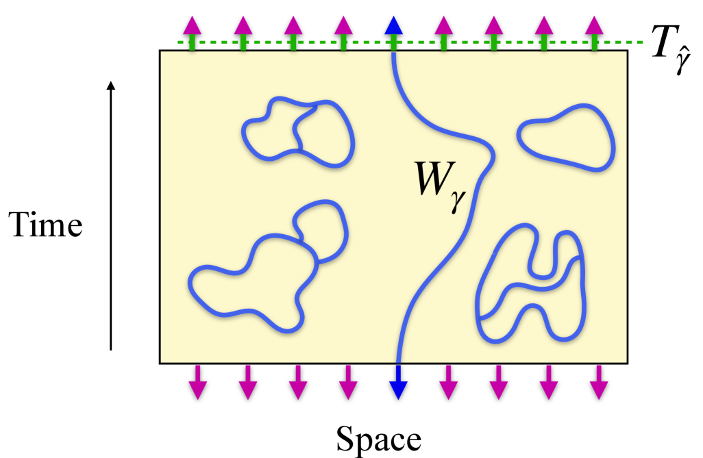
Figure 8: Wilson and ’t Hooft loops. The dual lattice curve, $T_{\hat{\gamma}}$, at the final time slice denotes a ’t Hooft loop. It generates an 1-form electric symmetry in the gauge theory and serves to distinguish between different topological sectors. States in different topological sectors are related to one another through the action of a non-contractible Wilson string, $W_{\gamma}$, which begins at the initial timeslice boundary and terminates at the final timeslice boundary.

Recall that the ’t Hooft operator $T_{\hat{\mathcal{C}}}$ measures the total electric flux penetrating the closed dual loop $\hat{\mathcal{C}}$. In a pure gauge theory without charge defects, Gauss’s law enforces that the net electric flux through any contractible loop must vanish. However, it imposes no constraint on the flux through a non-contractible surface. Consequently, states carrying different amounts of electric flux through homologically non-trivial surfaces belong to distinct topological superselection sectors of the gauge-theory Hilbert space. These sectors are related by “large gauge transformations” and cannot be connected by any local operator.

Since the ’t Hooft operator corresponds to a global symmetry operator of the spin chain, it follows that the distinct topological sectors of the gauge theory map directly onto the different global charge sectors of the spin chain. This exemplifies a well-known phenomenon: when a 1-form symmetry operator in the bulk gauge theory is pushed to the boundary, it manifests as a 0-form global symmetry in the edge theory.

III.2 Logical States

The structure of the bulk gauge wavefunction depends on two ingredients: $\mathbb{Z}_{N}$ charge selection rule, and initial state $|\Psi_{\rm in}\rangle$. Depending on which initial state we choose, the circuit dynamics, such as whether the charge information can be learned or not under weak measurements, can change. Without loss of generality, we define a set of initial states which are maximally robust in the sense that it protects the information leakage against measurements or decoherence. We shall refer to this as logical subspace of the spin chain. For $\mathbb{Z}_{N}$ symmetric circuits, this allows to encode precisely one qudit worth of information.

For example, consider the initial spin configuration given by the product state with definite local charges:

$$\ket{\psi_{0}}=\ket{j_{1}}|j_{2}\rangle\cdots\ket{j_{L}},$$ (50)

where we dropped multiplicity labels as they do not matter. Such a state loses its charge information quickly under local weak measurements. On the other hand, if the initial spin-chain state is prepared as a uniform superposition over all simultaneous $Z$-eigenstates with a fixed total charge $Q$,

$$\ket{\psi_{0}(Q)}=\frac{1}{N^{(L-1)/2}}\hskip-15.0pt\sum_{\begin{subarray}{c}j_{1}\cdots j_{L}\\ Q\equiv\sum_{i}j_{i}\textrm{ mod $N$}\end{subarray}}\hskip-15.0pt\ket{j_{1}}\cdots\ket{j_{L}}$$ (51)

then the resulting gauge state $\ket{\Phi_{g}(Q)}$ is a uniform superposition over all $\mathbb{Z}_{N}$ string-net configurations with initial and final time slices subject to the condition $T_{\hat{\gamma}}\ket{\Phi_{g}(Q)}=e^{2\pi iQ/N}\ket{\Phi_{g}(Q)}$.

The observation that product and scrambled states exhibit different levels of protection against charge measurements is the coherent version of the distinction between mixed states with and without strong-to-weak spontaneous symmetry breaking (SWSSB) [35, 61, 62, 63, 64, 65]. A product state with definite local charges is easily learned by charge measurements, whereas a scrambled state makes the same charge information difficult to access. Put differently, their response to a measurement channel (weakly symmetric) is sharply different [35]. In our setup, the circuit is initialized in a coherent SWSSB state, namely a pure state in which the charge is highly scrambled and thus enjoys enhanced protection against charge measurements. From this perspective, the charge purification transition corresponds to the restoration of strong symmetry.

States with different $Q$s are only distinguished by the total $\mathbb{Z}_{N}$ flux that crosses any surface at intermediate circuit time. They can be related to one another as follows

$$\ket{\Phi_{g}(Q)}=W_{\gamma}^{Q}\ket{\Phi_{g}(0)}$$ (52)

where $W_{\gamma}$ is a Wilson loop (a product of $X$ operators on the direct lattice) along a non-contractible open curve $\gamma$ connecting the two rough boundaries (see Fig. 8). $Q$ being an eigenvalue of ’t Hooft operator, $\ket{\Phi_{g}(Q)}$ are precisely the logical states of the $\mathbb{Z}_{N}$ surface code.

Accordingly, we define a logical subspace of the spin chain as follows

$$\mathcal{H}_{\text{logical}}=\mathrm{span}\{\ket{\psi_{0}(Q)}\,|\,Q=0,1,...,N-1\}.$$ (53)

This logical subspace can be protected against local errors because its circuit dynamics maps to the higher-dimensional topological bulk under decoherence, which has a finite noise threshold. More explicitly, consider a local symmetric quantum channel acting on the charge degrees of freedom, $\mathcal{E}^{t}(\cdot)=\prod_{k=1}^{L}\mathcal{E}^{t}_{k}(\cdot)$. Its action maps to the corresponding channel on every bulk link of the gauge wavefunction, $\prod_{\mu}\mathcal{E}_{\mu}\big(\cdot\big)$. Because the logical qudit of the surface code is stable against weak decoherence [34, 36, 37, 66], the corresponding logical spin states likewise retain their encoded information in this regime.

III.3 Coherent Information

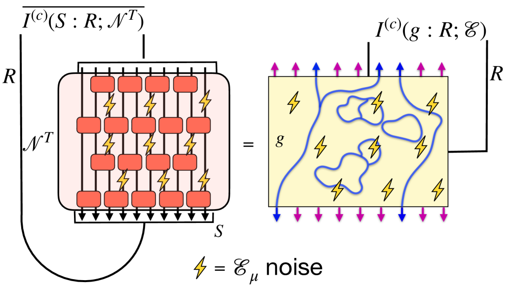
Figure 9: Equality of Coherent Information: Upon averaging over the multiplicity tensors in the large multiplicity limit, the coherent information of the spin chain evolving under the noisy symmetric circuit is precisely equal to the coherent information of the bulk surface code subjected to the same local noise.

Let us examine the robustness of the information encoded in the spin states $\{\ket{\psi_{0}(Q)}\}$ in more detail. To this end, it is useful to imagine coupling the spin chain $S$ to an external reference qudit $R$ whose Hilbert space dimension equals the number of distinct global charges of the spin chain. We can then prepare the composite spin chain + qudit system in a maximally entangled state

$$\ket{\Psi_{0}}_{SR}=\frac{1}{\sqrt{N}}\sum_{Q=0}^{N-1}\ket{\psi_{0}(Q)}_{S}\otimes\ket{Q}_{R}$$ (54)

The density matrix of the composite $SR$ system is $\rho_{SR}=|\Psi_{0}\rangle_{SR}\langle\Psi_{0}|_{SR}$ whereas the reduced density matrix of $S$ is found to be a classical mixture of all logical states

$$\rho_{S}=\frac{1}{N}\sum_{Q}|{\psi_{0}(Q)}\rangle_{S}\langle\psi_{0}(Q)|_{S}$$ (55)

The spin chain is then evolved using local unitary gates arranged in a bricklayer architecture, interleaved with local noise channels of the form $\mathcal{E}^{t}(\cdot)=\prod_{k=1}^{L}\mathcal{E}^{t}_{k}(\cdot)$. Let us denote the combined quantum channel after $T$ time steps by $\mathcal{N}^{T}$. The amount of distillable quantum information that can be extracted following the action of $\mathcal{N}^{T}$ is quantified by the coherent information [67, 68, 69, 70], defined as

$$I^{(c)}(S:R;\mathcal{N}^{T})=S(\mathcal{N}^{T}(\rho_{S}))-S(\mathcal{N}^{T}(\rho_{SR}))$$ (56)

where $S(\cdot)$ denotes the von Neumann entropy. Since the coherent information obeys the data processing inequality, $I^{(c)}(S:R;\mathcal{N}^{1}\circ\mathcal{N}^{2})\leq I^{(c)}(S:R;\mathcal{N}^{2})$, the amount of information that is lost as a consequence of noise can never be recovered by post-processing. As a consequence of the sub-additivity of entropy, it is easy to see that

$$-\log N\leq I^{(c)}(S:R;\mathcal{N}^{T})\leq\log N$$ (57)

A positive coherent information heralds distillable entanglement whereas a negative coherent information points to consumption of entanglement by the noisy channel.

Using the bulk boundary correspondence, we can write the final state of the spin chain as

$$\mathcal{N}^{T}(\rho_{S}) =\bigg(\bigotimes_{v}\bra{T_{v}}\bigg)E\rho_{\text{g}}E^{\dagger}\bigg(\bigotimes_{v}(\ket{T_{v}}\bigg)$$

$$\mathcal{N}^{T}(\rho_{SR}) =\bigg(\bigotimes_{v}\bra{T_{v}}\bigg)E\rho_{\text{gR}}E^{\dagger}\bigg(\bigotimes_{v}(\ket{T_{v}}\bigg)$$ (58)

where $\rho_{\text{gR}}=\prod_{\mu}\mathcal{E}_{\mu}(|\Phi_{\text{g}R}\rangle\langle\Phi_{\text{g}R}|)$, the state $\ket{\Phi_{\text{g}R}}$ is given by

$$\ket{\Phi_{\text{g}R}}=\frac{1}{\sqrt{N}}\sum_{Q=0}^{N-1}\ket{\Phi_{\text{g}}(Q)}\otimes\ket{Q}_{R}$$ (59)

and finally $\rho_{\text{g}}=\Tr_{\text{R}}\rho_{\text{gR}}$. Note that $\ket{\Phi_{\text{g}R}}$ is just a maximally entangled state between the logical subspace of the dynamically generated surface code and the reference system.

For now, let us consider the case where the channels $\mathcal{E}(\cdot)$ represent decoherence channels rather than measurement channels, so we do not have access to classical information carried by measurement register. We will investigate measurement-induced transitions in the next section. Our goal is to compute the coherent information averaged over realizations of the random multiplicity tensors. In the large-multiplicity limit-deep within the volume-law phase where replica symmetry is spontaneously broken-we show in Appendix. B that

$$\overline{S(\mathcal{N}^{T}(\rho_{S}))} =S(\mathcal{E}(\rho_{g}))$$

$$\overline{S(\mathcal{N}^{T}(\rho_{SR}))} =S(\mathcal{E}(\rho_{gR}))$$ (60)

namely, the averaged von Neumann entropy of the boundary state evolved under the quantum channel $\mathcal{N}^{T}$ equals the bulk von Neumann entropy of the corresponding surface-code state evolved under the linkwise decoherence channel $\mathcal{E}=\prod_{\mu}\mathcal{E}_{\mu}$. Consequently, the averaged coherent information of the $\mathbb{Z}_{N}$-symmetric spin chain is precisely equal to the coherent information of the bulk surface code:

$$\overline{I^{(c)}(S:R;\mathcal{N}^{T})} =I^{(c)}(g:R;\mathcal{E})$$ (61)

For the $\mathbb{Z}_{N}$ surface code, it is well established that the coherent information remains approximately constant at $\log N$ in the regime of weak decoherence, reflecting perfect recoverability of the encoded logical information. This robustness is directly inherited by the boundary spin chain: the logical qudit encoded in the spin states $\{\ket{\psi_{0}(Q)}\}$ remains protected against local errors induced by decoherence.

IV $\mathbb{Z}_{N}$ Charge Sharpening Transition

Charge sharpening is a measurement-induced phase transition in which an initial spin state, prepared as a superposition of multiple global charge sectors, collapses onto a single, definite charge sector once the (rate) strength of (projective) weak measurements becomes sufficiently large. A natural diagnostic for detecting this transition is the average variance of the global charge or symmetry operator. For the case $G=\mathbb{Z}_{N}$, each element of the group is generated by a single element $a$ with $a^{N}=e$. Thus, suffices to consider the variance of $V(a)=\prod_{k=1}^{L}Z_{k}=:Z_{\text{tot}}$ where $Z_{k}$ is the generalized Pauli operator at site $k$. Since $Z_{\text{tot}}$ is unitary, its variance at time $t$, conditioned on measurement outcomes $\bm{s}=\{s_{\mu}\}$ is simply given by

$$\textrm{Var}[Z_{\text{tot}}]^{\bf{s}}_{t}: =\langle|Z_{\text{tot}}-\langle Z_{\text{tot}}\rangle_{\mathbf{s},t}|^{2}\rangle_{\mathbf{s},t}$$

$$=1-|\langle Z_{\text{tot}}\rangle_{\mathbf{s},t}|^{2}$$ (62)

where $\langle\cdot\rangle_{\mathbf{s},t}$ denotes the normalized expectation value with respect to the spin chain state $\ket{\psi^{\mathbf{s}}(t)}$ at time $t$ for a specific trajectory of measurement outcomes $\bm{s}$. If the initial state $\ket{\psi_{0}}$ is chosen to maximize the charge variance $\textrm{Var}[Z_{\text{tot}}]_{0}=1$, then charge sharpening occurs when $\textrm{Var}[Z_{\text{tot}}]^{\bf{s}}_{t}\approx 0$, indicating that the spin chain has collapsed to a definite global charge sector. Conversely, if $\textrm{Var}[Z_{\text{tot}}]={\cal O}(1)$, the final state retains multiple charge sectors and the global charge remains fuzzy.

This setup involves two layers of randomness: (1) the local multiplicity tensors of the circuit are independently drawn from a random ensemble, and (2) the measurement outcomes $\bm{s}$ are random in accordance with the Born rule. Since we are interested in typical behaviour of the system, we need to average over both sources of randomness but the order of averaging is crucial since the Born probabilities themselves depend on the sampled multiplicity tensors.

We first average $\textrm{Var}[Z_{\text{tot}}]^{\bf{s}}_{t}$ over the post measurement ensemble $\{\ket{\psi^{\bf{s}}(t)}\}$. Each such trajectory occurs with probability $p^{\bf{s}}(t)=\innerproduct{\psi^{\bf{s}}(t)}{\psi^{\bf{s}}(t)}$. In the case of projective measurements, we must average over both the measurement locations and the measurement outcomes, whereas in the case of weak measurements, we only average over the measurement outcomes. We denote the average over measurement outcomes $\bm{s}$ using double brackets:

$$\langle\hskip-2.0pt\langle\textrm{Var}[Z_{\text{tot}}]\rangle\hskip-2.0pt\rangle_{t} =\sum_{\bf{s}}p^{\bf{s}}(t)\textrm{Var}[Z_{\text{tot}}]^{\textbf{s}}_{t}$$

$$=1-\sum_{\bf{s}}p^{\bf{s}}(t)|\langle Z_{\text{tot}}\rangle_{\mathbf{s},t}|^{2}$$ (63)

We then perform a second average over the ensemble of random multiplicity tensors, denoted by $\overline{\cdots}$. The resulting quantity is:

$$\overline{\langle\hskip-2.0pt\langle\textrm{Var}[Z_{\text{tot}}]\rangle\hskip-2.0pt\rangle}_{t}=1-\overline{\langle\hskip-2.0pt\langle|\langle Z_{\text{tot}}\rangle_{\mathbf{s},t}|^{2}\rangle\hskip-2.0pt\rangle}$$ (64)

Since this quantity involves a measurement average of a non-linear function of the state, it is capable of detecting the charge sharpening transition. In particular, in the charge fuzzy phase, we expect that $\overline{\langle\hskip-2.0pt\langle\textrm{Var}[Z_{\text{tot}}]\rangle\hskip-2.0pt\rangle}_{t}=\mathcal{O}(1)$ upto timescales $t\sim L$ whereas in the charge- harp phase, we expect that $\overline{\langle\hskip-2.0pt\langle\textrm{Var}[Z_{\text{tot}}]\rangle\hskip-2.0pt\rangle}_{t}\approx 0$ already at $t\sim\mathcal{O}(1)$. Evidently, an equivalent diagnostic for the sharpening transition is the quantity

$$\overline{\langle\hskip-2.0pt\langle|\langle Z_{\text{tot}}\rangle_{\mathbf{s},t}|^{2}\rangle\hskip-2.0pt\rangle}=\sum_{\bf{s}}\overline{\Bigg[\frac{|\matrixelement{\psi^{\mathbf{s}}(t)}{Z_{\text{tot}}}{\psi^{\mathbf{s}}(t)}|^{2}}{\innerproduct{\psi^{\mathbf{s}}(t)}{\psi^{\mathbf{s}}(t)}}\Bigg]}$$ (65)

which displays precisely the opposite behaviour, namely it remains approximately $0$ upto times $t\sim L$ in the charge fuzzy phase whereas in the charge sharp phase it rapidly saturates to 1 on a timescale $t\sim\mathcal{O}(1)$. In the following, we demonstrate how this order parameter is evaluated within the gauge theory and explain the nature of the associated bulk transition.

IV.1 Gauge Theoretical Description

Using the bulk-boundary correspondence, the final state of the spin chain may be expressed as $\ket{\psi^{\bf{s}}(t)}=\bigotimes_{v}(\bra{T_{v}})E\ket{\Phi^{\bf{s}}_{\text{g}}}$ where $\ket{\Phi^{\bf{s}}_{\text{g}}}=\tilde{K}_{\bf{s}}\ket{\Phi_{\text{g}}}$ is the (unnormalized) gauge wavefunction conditioned on measurement outcomes $\bf{s}$. Using the intertwining identity in Eq. (48), the action of the symmetry operator $Z_{\text{tot}}$ on the spin chain can be replaced by that of a non-contractible ’t Hooft loop $T_{\hat{\gamma}}$ which threads the rough boundary of the bulk gauge theory at the final timeslice. In Appendix. C, we show that averaging over the multiplicity tensors in the large-multiplicity limit yields the simple equation

$$\overline{\langle\hskip-2.0pt\langle|\langle Z_{\text{tot}}\rangle_{\mathbf{s},t}|^{2}\rangle\hskip-2.0pt\rangle} =\sum_{\bf{s}}p({\bf{s}})\Bigg|\frac{\bra{\Phi^{\bm{s}}_{\text{g}}}{T_{\hat{\gamma}}}\ket{\Phi^{\bm{s}}_{\text{g}}}}{\innerproduct{\Phi^{\bm{s}}_{\text{g}}}{\Phi^{\bm{s}}_{\text{g}}}}\Bigg|^{2}$$

$$=\langle\hskip-2.0pt\langle|T_{\hat{\gamma}}|^{2}\rangle\hskip-2.0pt\rangle$$ (66)

where now $p({\bf{s}})=\innerproduct{\Phi^{\bm{s}}_{\text{g}}}{\Phi^{\bm{s}}_{\text{g}}}$. Thus, the diagnostic for sharpening is precisely the measurement average of the squared expectation value of a non-contractible ’t Hooft operator. We choose the initial state to be the uniform superposition of logical spin states defined in (51)

$$\ket{\psi_{0}}=\frac{1}{\sqrt{N}}\sum_{Q=0}^{N-1}\ket{\psi_{0}(Q)}$$ (67)

This state is the simultaneous +1 eigenstate of all $\mathbb{Z}_{N}$ Pauli $X$ operators. This state satisfies $\textrm{Var}[Z_{\text{tot}}]_{0}=1$ and, since it is a logical state, it is robust to the errors induced by measurements. The corresponding gauge state is thus given by

$$\ket{\Phi^{\bm{s}}_{\text{g}}}=\sum_{Q=0}^{N-1}\ket{\Phi^{\bm{s}}_{\text{g}}(Q)}$$ (68)

where $\ket{\Phi^{\bm{s}}_{\text{g}}(Q)}=\tilde{K}_{\bm{s}}\ket{\Phi_{\text{g}}(Q)}$ and we’ve dropped the normalization. Since the measurement Kraus operators commute with $T_{\hat{\gamma}}$, and since $T_{\hat{\gamma}}\ket{\Phi^{\bm{s}}_{\text{g}}(Q)}=\omega^{Q}\ket{\Phi^{\bm{s}}_{\text{g}}(Q)}$ where $\omega=e^{2\pi i/N}$, it follows that

$$\langle\hskip-2.0pt\langle|T_{\hat{\gamma}}|^{2}\rangle\hskip-2.0pt\rangle=\sum_{\bf{s}}\bigg(\sum_{Q^{\prime}=0}^{N-1}\mathcal{Z}[\textbf{s},Q^{\prime}]\bigg)\Bigg|\frac{\sum_{Q=0}^{N-1}\omega^{Q}\mathcal{Z}[\textbf{s},Q]}{\sum_{Q=0}^{N-1}\mathcal{Z}[\textbf{s},Q]}\Bigg|^{2}$$ (69)

where we’ve defined $\mathcal{Z}[\textbf{s},Q]=\innerproduct{\Phi^{\bm{s}}_{\text{g}}(Q)}{\Phi^{\bm{s}}_{\text{g}}(Q)}$. Evaluating this quantity reduces to computing the Born probabilities $\mathcal{Z}[\textbf{s},Q]$ for observing measurement outcomes $\bf{s}$ for the logical state $\ket{\Phi_{\text{g}}(Q)}$. Below, we show that these probabilities can be conveninetly re-expressed as the partition function of a disordered statistical-mechanics model.

IV.2 Local Charge Sharpening

We can also consider the fluctuation of charge contained in a local region of the spin chain. For instance, consider a subregion $A$ of the spin chain of length $l_{A}$. The associated $\mathbb{Z}_{N}$ symmetry operator is given by $Z_{A}=\prod_{k\in A}Z_{k}$ respectively. Its variance is

$$\mathrm{Var}[Z_{A}]^{\mathbf{s}}_{t}=1-|\langle Z_{A}\rangle_{\mathbf{s},t}|^{2}$$ (70)

Once again, averaging the squared expectation $|\langle Z_{A}\rangle_{\mathbf{s},t}|^{2}$ over all measurement outcomes and the ensemble of random multiplicity tensors yields

$$\overline{\langle\hskip-2.0pt\langle|\langle Z_{\text{tot}}\rangle_{\mathbf{s},t}|^{2}\rangle\hskip-2.0pt\rangle} =\sum_{\bf{s}}p({\bf{s}})\Bigg|\frac{\bra{\Phi^{\bm{s}}_{\text{g}}}{T_{\hat{\gamma}_{A}}}\ket{\Phi^{\bm{s}}_{\text{g}}}}{\innerproduct{\Phi^{\bm{s}}_{\text{g}}}{\Phi^{\bm{s}}_{\text{g}}}}\Bigg|^{2}$$

$$=\langle\hskip-2.0pt\langle|T_{\hat{\gamma}_{A}}|^{2}\rangle\hskip-2.0pt\rangle$$ (71)

where $T_{\hat{\gamma}_{A}}$ is an open ’t Hooft string inserted at the final timeslice which threads across subregion $A$. This can be interpreted as creating a pair of magnetic fluxes on the ends of subregion $A$. Thus the expectation value $\langle T_{\gamma_{A}}\rangle$ is expected to behave as a two point correlator.

IV.3 Random Bond Clock Models

In this section, we demonstrate how the probabilities $\innerproduct{\Phi^{\bm{s}}_{\text{g}}(Q)}{\Phi^{\bm{s}}_{\text{g}}(Q)}$ can be reexpressed as partition functions for disordered clock models. We take the weak measurement Kraus operators to be

$$\tilde{K}_{s} ={\sum_{j=0}^{N-1}\sqrt{p_{j;s}}|j\rangle\langle j|}$$ (72)

The logical surface code state $\ket{\Phi_{\text{g}}(Q)}$ is a uniform superposition of all allowed string-net configurations satisfying $T_{\hat{\gamma}}\ket{\Phi^{\bm{s}}_{\text{g}}(Q)}=\omega^{Q}\ket{\Phi^{\bm{s}}_{\text{g}}(Q)}$. A convenient way to parametrize these states is in terms of a $\mathbb{Z}_{n}$-valued flow variable $\bf{k}$ defined on the links of the lattice, representing the eigenvalue of the Pauli $Z$ operator associated with each link. In this notation, we can write

$$\ket{\Phi_{\text{g}}(Q)}=\sum_{\begin{subarray}{c}\bf{k}|\nabla\cdot\bf{k}=0\\ \hat{\gamma}(\bf{k})=Q\end{subarray}}\ket{\bf{k}}$$ (73)

where the lattice divergence condition $\nabla\cdot\bf{k}=0\mod N$ enforces Gauss’ law on each vertex and $\hat{\gamma}(\bf{k})=Q$ fixes the $\mathbb{Z}_{n}$ flux threading the non-contractible cycle $\hat{\gamma}$ to be $Q$, namely $\sum_{\mu\perp\hat{\gamma}}k_{\mu}=Q\mod N$. Acting on this state with the weak measurement operators then yields

$$\prod_{\mu}\tilde{K}_{s_{\mu}}\ket{\Phi_{\text{g}}(Q)} =\sum_{\begin{subarray}{c}\textbf{k}|\nabla\cdot\textbf{k}=0\\ \hat{\gamma}(\textbf{k})=Q\end{subarray}}\prod_{\mu}\sqrt{p_{k_{\mu};s_{\mu}}}\ket{\bf{k}}$$ (74)

It then follows that

$$\mathcal{Z}[\textbf{s};Q]=\innerproduct{\Phi^{\bm{s}}_{\text{g}}(Q)}{\Phi^{\bm{s}}_{\text{g}}(Q)}=\sum_{\begin{subarray}{c}\textbf{k}|\nabla\cdot\textbf{k}=0\\ \hat{\gamma}(\textbf{k})=Q\end{subarray}}\prod_{\mu}p_{k_{\mu};s_{\mu}}$$ (75)

For clock type weak measurements characterized by the properties, $p_{j;s}\equiv p_{j-s\mod N}$ and $p_{k}=p_{-k\mod N}$, $\mathcal{Z}[\textbf{s};Q]$ precisely corresponds to the current-loop representation of a $\mathbb{Z}_{N}$ clock model clock model with quenched bond disorder $\{s_{\mu}\}$, restricted to a fixed homology sector labeled by $Q$. To see this, we first write $p_{k}=\frac{e^{\alpha_{k}}}{\mathcal{N}}$, where $\mathcal{N}=\sum_{k}e^{\alpha_{k}}$, and define the discrete $\mathbb{Z}_{N}$ Fourier transform of $\alpha_{k}$ as follows

$$\alpha_{k} =\sum_{m=0}^{[N/2]}\beta_{m}\cos{\frac{2\pi km}{N}}$$ (76)

Only cosine modes appear due to the assumed parity symmetry $p_{k}=p_{-k\mod N}$. It then follows that $p_{j;s}=\frac{1}{\mathcal{N}}\exp{\sum_{m=0}^{[N/2]}\beta_{m}\cos{\frac{2\pi(j-s)m}{N}}}$. Next we solve the divergence free condition by introducing $\mathbb{Z}_{N}$ spins $\theta_{p}$ on each plaquette of the lattice and defining

$$k_{\langle p_{1}\rightarrow p_{2}\rangle} =\theta_{p_{1}}-\theta_{p_{2}}\mod N$$ (77)

Here $\langle p_{1}\rightarrow p_{2}\rangle$ denotes the unique oriented dual lattice link that cuts the direct lattice link $\mu$ from left to right. Such flows satisfy both $\nabla\cdot\bf{k}=0$ and $\hat{\gamma}(\bf{k})=0$. To generate a non-trivial $\mathbb{Z}_{n}$ flux through $\hat{\gamma}$, we may choose an arbitrary direct-lattice loop $\gamma$ connecting the initial and final timeslice boundaries and add a flow $Q$ along $\gamma$. This is equivalent to modifying the quenched background configuration by subtracting $Q$ from every link along $\gamma$.

$$s^{Q}_{\mu}=\begin{cases}s^{0}_{\mu}-Q\quad\mu\in\gamma\\ s^{0}_{\mu}\quad\mu\notin\gamma\end{cases}$$ (78)

This then allows us to write (upto normalization)

$$\mathcal{Z}[\textbf{s}^{Q}] =\sum_{\{\theta_{p}\}}\exp{-H[\{\theta_{p}\};\textbf{s}^{Q}]}$$ (79)

$$H[\{\theta_{p}\};\textbf{s}^{Q}] =-\sum_{\langle p_{1},p_{2}\rangle}\sum_{m=0}^{[N/2]}\beta_{m}$$

$$\times\cos{\frac{2\pi m\big(\theta_{p_{1}}-\theta_{p_{2}}-s^{Q}_{\langle p_{1},p_{2}\rangle}\big)}{N}}$$ (80)

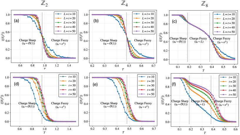
Figure 10: Numerical results for $\langle|T_{\hat{\gamma}}|^{2}\rangle$: We study charge sharpening dynamics in $\mathbb{Z}_{2}$ (left), $\mathbb{Z}_{4}$ (middle), and $\mathbb{Z}_{8}$ (right) symmetric circuits subject to the weak measurement model of Eq. (83). The measurement strength is controlled by a single effective parameter $T$, which we interpret as a temperature. We evaluate $\langle|T_{\hat{\gamma}}|^{2}\rangle$ using the worm algorithm; this quantity directly diagnoses the sharpening transition. When $\langle\hskip-2.0pt\langle|T_{\hat{\gamma}}|^{2}\rangle\hskip-2.0pt\rangle\approx 0$, the global charge remains fuzzy whereas when $\langle\hskip-2.0pt\langle|T_{\hat{\gamma}}|^{2}\rangle\hskip-2.0pt\rangle\approx 1$, the charge sharpens. Throughout $L$ denotes the size of the spin chain and $t$ denotes time. Figures (a), (b) and (c) plot $\langle\hskip-2.0pt\langle|T_{\hat{\gamma}}|^{2}\rangle\hskip-2.0pt\rangle$ for $L=t$. Note that for large $T$, when measurements are weak, the global charge remains fuzzy whereas for small $T$, when measurements are strong, global charge sharpens rapidly. Notably, in the $\mathbb{Z}_{8}$ case we find a clear regime where the curves collapse for all $L=t$, a hallmark of the QLRO (Coulomb) phase. Figures (d), (e) and (f) plot $\langle\hskip-2.0pt\langle|T_{\hat{\gamma}}|^{2}\rangle\hskip-2.0pt\rangle$ for fixed system size $L=30$ and varying circuit time $t$.

This is precisely the partition function of a $\mathbb{Z}_{N}$ clock model with quenched bond disorder $\{s_{\mu}\}$ determined by the measurement outcomes and couplings $\beta_{m}$ determined by the measurement channel. Note that the net effect of non-trivial flux $Q$ is to impose a $(-Q)$-twisted boundary condition along the path $\gamma$ in the clock model. This introduces a form of topological frustration that energetically biases the system toward one topological sector over the rest.

Finally, note that the expectation value of an open ’t Hooft string $T_{\hat{\gamma}_{A}}$ along subregion $A$ can be written as

$$\bra{\Phi^{\bm{s}}_{\text{g}}}{T_{\hat{\gamma}_{A}}}\ket{\Phi^{\bm{s}}_{\text{g}}}=\sum_{\{\theta_{p}\}}\omega^{\theta_{p_{1}}-\theta_{p_{2}}}e^{-H[\{\theta_{p}\};\textbf{s}^{Q}]}$$ (81)

where ${p_{1}}$ and $p_{2}$ are the plaquettes at the endpoints of the dual lattice curve $\hat{\gamma}_{A}$. This expression is simply the (disconnected) spin–spin correlation function of the disordered clock model for a fixed realization of the quenched couplings $\bf{s}$. It follows that

$$\langle\hskip-2.0pt\langle|T_{\hat{\gamma}_{A}}|^{2}\rangle\hskip-2.0pt\rangle=[\langle\omega^{\theta_{p_{1}}-\theta_{p_{2}}}\rangle|^{2}]$$ (82)

where in the RHS $\langle\cdots\rangle$ now denotes a thermal average at fixed disorder and $[\cdots]$ denotes an average over the disorder ensemble.

IV.4 Phase Diagrams

$\mathbb{Z}_{N}$ clock models in 2 dimensions have been studied extensively in the literature since they interpolate between the Ising model ($N=2$) and the XY model ($N\rightarrow\infty$). Notable intermediate cases include the three-state Potts model $(N=3)$ and the Ashkin-Teller model $(N=4)$. These models display a rich phase diagram owing to their dihedral symmetry $D_{N}=\mathbb{Z}_{N}\rtimes\mathbb{Z}^{P}_{2}$. In the absence of disorder, it has long been known that the phase diagram of the 2D clock model qualitatively changes with increasing $N$. In particular, for $2\leq N\leq 4$, the $\mathbb{Z}_{N}$ clock model exhibits only two phases: an ordered ferromagnetic phase at low temperature and a disordered paramagnetic phase at high temperature, separated by a single critical point. On the other hand, for $N>4$, the $\mathbb{Z}_{N}$ clock model exhibits three different phases: an ordered phase, an disordered phase, and an intervening quasi–long-range-ordered (QLRO) critical phase. [71, 72, 73, 74, 75, 76, 77, 78, 79, 80]. Within this intermediate phase, vortices remain irrelevant and furthermore the $\mathbb{Z}_{N}$ locking terms also become irrelevant, leaving behind an effective Gaussian spin-wave theory with an emergent $U(1)$ symmetry. The existence of the QLRO phase follows from general renormalization group arguments: it does not rely on any fine tuned choice of $\beta_{m}$ couplings. These couplings merely affect nonuniversal properties, such as the precise locations of the two critical points, without altering the qualitative structure of the phase diagram.

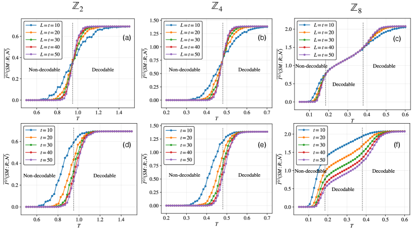
Figure 11: Numerical results for the coherent information $\overline{I^{(c)}(SM:R;\mathcal{N})}$: We compute the measurement-averaged coherent information for $\mathbb{Z}_{2}$ (left), $\mathbb{Z}_{4}$ (middle), and $\mathbb{Z}_{8}$ (right) symmetric circuits subjected to the weak measurement model of Eq. (83). The coherent information is evaluated using the analytic form derived in Eq. (IV.5) and sampled numerically via the worm algorithm. Panels (a), (b), and (c) show $\overline{I^{(c)}(SM\!:\!R;\mathcal{N})}$ along the line $L=t$, while panels (d), (e), and (f) display $\overline{I^{(c)}(SM\!:\!R;\mathcal{N})}$ for a fixed system size $L=30$ as a function of circuit time $t$. For large $T$ (weak measurements), the encoded quantum information remains robust and the monitored symmetric circuit acts as a stable memory. In contrast, for small $T$ (strong measurements), the information stored in the spin chain is rapidly erased. The coherent information exhibits a sharp transition at the same critical measurement strength as the charge-sharpening transition, confirming that learnability of the global charge coincides with a decodability transition of the emergent code.

The fate of this intermediate QLRO phase in the presence of quenched disorder has been heavily debated [81]. It is known that sufficiently strong disorder destroys all signatures of the QLRO phase. However, in our case, we are interested in computing expectation values of the form given in Eq. (69) for which the disorder distribution $P(\bf{s})$ is effectively proportional to the partition function itself $\mathcal{Z}[\bf{s}]$. This ties the temperature to the disorder and confines us to a special locus known as the Nishimori line. The Nishimori line is very special because the disordered model acquires an effective local $\mathbb{Z}_{N}$ symmetry [82, 83]. This is entirely unsurprising in our context, since the partition functions we evaluate encode amplitudes of an underlying gauge wavefunction. Along the Nishimori line, it is generally expected that the qualitative structure of the phase diagram matches that of the clean $\mathbb{Z}_{N}$ clock model [84, 85]. Which phase the system occupies ultimately depends on the weak measurement channel and the choice of parameters $p_{k}$. Below, we make a concrete choice for these parameters and numerically confirm the emergence of all three phases along the Nishimori line for $N>4$ as the strength of the measurement is varied.

IV.4.1 Numerics

Here we briefly outline how to compute the quantity $\langle\hskip-2.0pt\langle|T_{\hat{\gamma}}|^{2}\rangle\hskip-2.0pt\rangle$ given in Eq. (69). We consider the simple weak measurement model with parameters

$$p_{k}=\frac{\exp{\frac{1}{T}\cos{\frac{2\pi k}{N}}}}{\mathcal{N}}$$ (83)

where $\mathcal{N}$ is a normalization constant. In the notation of Eq. (79), this corresponds to choosing a single nonzero coupling $\beta_{1}=\frac{1}{T}$ with all other $\beta_{m\neq 1}=0$. The parameter $T$ plays the role of an effective “temperature” controlling the strength of the weak measurement. For small $T$, $p_{k}$ is sharply peaked around $k=0$ approaching the projective measurement limit. In this regime, measurements profoundly disrupt the state and the global charge sharpens rapidly. On the other hand, for large $T$, $p_{k}\approx\frac{1}{N}$ corresponding to the no measurement limit.

To proceed, note that the quantity $P(\textbf{s},Q)=\mathcal{Z}[\textbf{s},Q]/(\sum_{Q^{\prime}=0}^{N-1}\mathcal{Z}[\textbf{s},Q^{\prime}])$ is just a winding number probability in the presence of quenched disorder s. These probabilities can be computed efficiently using the worm algorithm [86, 87]. The algorithm samples configurations in the high-temperature (current-loop) expansion of the classical statistical model, in the form given in  Eq. (75).

Flow configurations obey a divergence-free constraint $\nabla\cdot\mathbf{k}=0$, which the worm algorithm temporarily relaxes by introducing a pair of defect sites—the head and tail of the worm—that violate this constraint. The Markov chain then propagates the head through local moves weighted by the appropriate Boltzmann factor. When the head returns to the tail, the defects annihilate and the configuration again satisfies all constraints of the original model. Observables are obtained by averaging over these closed-loop configurations, while the intermediate open-worm configurations ensure ergodic sampling of correlation functions. Importantly, the algorithm suffers from minimal critical slowing down and is ergodic across all winding-number sectors, making it highly efficient for computing the winding probabilities $P(\textbf{s},Q)$ (see [86, 87] for more details).

Since our focus is on bulk phase transitions of the statistical mechanical model, we may impose periodic boundary conditions in both lattice directions. The horizontal winding sectors can be safely traced over, as they have no physical meaning in the surface code picture due to the rough boundaries at the initial and final timeslice. In the limit of large lattice sizes, the bulk phase transitions of the Stat model with periodic boundaries coincide with those of the original surface code geometry, since boundary effects become completely negligible.

In Appendix. F, we analyse the scaling of the partition function $\mathcal{Z}[\textbf{s};Q]$ with $L$ and $t$ (the dimensions of the lattice) using high and low temperature expansions together with a Gaussian mean-field ansatz appropriate for the QLRO phase. If the frustration of the bonds s along the non-contractible closed curve $\hat{\gamma}$ is given by $Q^{\prime}=\hat{\gamma}(\textbf{s})$, so that $\mathcal{Z}[\textbf{s};Q^{\prime}]$ contains no topological frustration, we find that:

$$\mathcal{Z}[\textbf{s};Q]\sim\begin{cases}\mathcal{Z}[\textbf{s};Q^{\prime}]+c_{1}(Q-Q^{\prime})Te^{-\alpha L}&\text{Disordered}\\ e^{-c_{2}(Q-Q^{\prime})\frac{t}{L}}\mathcal{Z}[\textbf{s};Q^{\prime}]&\text{QLRO}\\ e^{-c_{3}(Q-Q^{\prime})T}\mathcal{Z}[\textbf{s};Q^{\prime}]&\text{Ordered}\end{cases}$$ (84)

This predicts sharpening timescales of the form

$$t_{\#}\sim\begin{cases}e^{\alpha L}&\text{Disordered}\\ L&\text{QLRO}\\ \mathcal{O}(1)&\text{Ordered}\end{cases}$$ (85)

We verify these predictions numerically in Fig. 10.

IV.4.2 Confinement Transition

We can also consider the case of local sharpening. It should be immediate that in the disordered and QLRO phases, local charges should never fully sharpen. Using the fact that the sharpening order parameter is precisely the disorder-averaged squared spin–spin correlator (see Eq. (82)), we immediately infer its scaling in the three phases:

$$\langle\hskip-2.0pt\langle|T_{\hat{\gamma}_{A}}|^{2}\rangle\hskip-2.0pt\rangle=\begin{cases}e^{-cL_{A}}\qquad\text{{Disordered}}\\ L_{A}^{-2\Delta}\qquad\text{{QLRO}}\\ \mathcal{O}(1)\qquad\text{{Ordered}}\end{cases}$$ (86)

This behavior admits a transparent interpretation in the gauge-theoretic picture. Recall that the ensemble of post-measurement gauge states is given by

$$\ket{\Phi^{\bf{s}}_{\text{g}}}=\sum_{\begin{subarray}{c}\textbf{k}|\nabla\cdot\textbf{k}=0\\ \hat{\gamma}(\textbf{k})=Q\end{subarray}}\prod_{\mu}\sqrt{p_{k_{\mu};s_{\mu}}}\ket{\bf{k}}$$ (87)

At large $T$ (low measurement strength), the weights $p_{k_{\mu};s_{\mu}}$ are broad so $\ket{\Phi^{\bf{s}}_{\text{g}}}$ is acoherent sum over essentially all string-net configurations. This is a long range entangled state and electrically deconfined state. Equivalently, since the expectation value of the open ’tHooft string decays exponentially $\langle\hskip-2.0pt\langle|T_{\hat{\gamma}_{A}}|^{2}\rangle\hskip-2.0pt\rangle\approx e^{-cL_{A}}$, implying linear confinement of magnetic fluxes.

On the other hand, for very low $T$, measurements become projective and $\ket{\Phi^{\bf{s}}_{\text{g}}}$ approaches a product state $\ket{\bf{s}}$ that possesses short range entanglement and is electrically confined. Equivalently since $\langle\hskip-2.0pt\langle|T_{\hat{\gamma}_{A}}|^{2}\rangle\hskip-2.0pt\rangle\approx\mathcal{O}(1)$, magnetic fluxes proliferate in this phase and states are magnetically deconfined. Thus, the ensemble of measured states undergoes a transition from electric deconfinement to electric confinement. In the intermediate QLRO phase, the ’t Hooft operator decays as a power law, the ’t Hooft string decays as a power law $\langle\hskip-2.0pt\langle|T_{\hat{\gamma}_{A}}|^{2}\rangle\hskip-2.0pt\rangle\approx e^{-cL_{A}}$, indicating that the state supports gapless modes. This corresponds to a Coulomb phase with emergent photons. Recall that in this regime the partition function is governed by an effective Gaussian spin-wave theory, whose long-wavelength excitations capture smooth fluctuations of the coarse-grained spin field. Since these spin variables encode magnetic flux, the emergent photons can be understood as collective, long-wavelength oscillations of local magnetic fluxes.

IV.5 Decodability Transition

Upto this point, we have interpreted the sharpening transition as a learnability transition: a change in how quickly local charge measurements reveal the global charge. We now recast the same phenomenon as a decodability transition, in which the logical information encoded in terms of the initial spin chain states given in Eq. (53) is destroyed by the monitored symmetric circuit.

In the charge-fuzzy phase, the global charge remains hidden, and the monitored symmetric circuit functions as an effective quantum memory: the logical qudit encoded in the global charge sector is protected against the local measurement-induced noise. By contrast, in the charge-sharp phase, the global charge is revealed rapidly, and the same measurement process simultaneously erases the logical information stored in the initial spin-chain state. Viewed through this lens, charge sharpening is precisely the transition at which the logical qudit ceases to be decodable under the monitored symmetric dynamics.

To this end, we consider the coherent information of the spin chain evolving under the combined unitary+measurement channel. A crucial subtlety is that the measurement record constitutes classical information and must be retained explicitly. Consequently, the effective quantum channel that acts on the spin chain $S$ is really given by

$$\mathcal{N}(\rho_{S})=\sum_{\textbf{s}}{\mathcal{N}}_{s}\rho_{S}\mathcal{N}^{\dagger}_{\textbf{s}}\otimes|s\rangle\langle s|_{M}$$ (88)

where $\mathcal{N}_{\textbf{s}}$ denotes the monitored circuit evolution with measurement outcomes conditioned to be s and $|\mathbf{s}\rangle\langle\mathbf{s}|_{M}$ denotes the state of the classical measurement register $M$ that stores the full trajectory of measurement outcomes.

Let us choose a reference $R$ that is maximally entangled with the logical states of the spin chain, given in Eq. (53).

$$\ket{\Psi_{0}}_{SR}=\frac{1}{\sqrt{N}}\sum_{Q=0}^{N-1}\ket{\psi_{0}(Q)}_{S}\otimes\ket{Q}_{R}$$ (89)

Under the quantum channel, this state evolves to

$$\rho_{SRM}=\sum_{\textbf{s}}{\mathcal{N}}_{s}|\Psi_{0}\rangle_{SR}\langle\Psi_{0}|_{SR}\mathcal{N}^{\dagger}_{\textbf{s}}\otimes|s\rangle\langle s|_{M}$$ (90)

The coherent information, which quantifies the distillable quantum information preserved by the channel, given access to the measurement outcomes, is

$$I^{(c)}(SM:R;\mathcal{N})=S(\mathcal{N}(\rho_{SM}))-S(\mathcal{N}(\rho_{SRM}))$$ (91)

Again, averaging this quantity over random multiplicity tensors in the large bond dimension limit allows us to express this quantity as the coherent information of the bulk surface code (see Sec. B)

$$\overline{I^{(c)}(SM:R;\mathcal{N})}=S(\mathcal{E}(\rho_{gM}))-S(\mathcal{E}(\rho_{gRM}))$$ (92)

where $\mathcal{E}$ now only contains measurement channels and not unitary evolution. The initial state of the reference $R$ and the gauge theory $g$ is given by

$$\ket{\Phi_{\text{g}R}}=\frac{1}{\sqrt{N}}\sum_{Q=0}^{N-1}\ket{\Phi_{\text{g}}(Q)}\otimes\ket{Q}_{R}$$ (93)

Recall again that $\ket{\Phi_{\text{g}}(Q)}$ are just the surface code logical states. We can now compute the above entropies in the bulk surface code and show that it undergoes a transition. In terms of the partition functions $\mathcal{Z}[\textbf{s},Q]=\innerproduct{\Phi^{\bm{s}}_{\text{g}}(Q)}{\Phi^{\bm{s}}_{\text{g}}(Q)}$, it is easily shown that

$$S(\mathcal{E}(\rho_{gMR})) =-\sum_{\textbf{s}}\mathcal{Z}[\textbf{s}]\log\mathcal{Z}[\textbf{s}]$$ (94)

$$S(\mathcal{E}(\rho_{gM})) =-\sum_{\textbf{s},Q}\frac{\mathcal{Z}[\textbf{s},Q]}{N}\log\frac{\mathcal{Z}[\textbf{s},Q]}{N}$$ (95)

where $\mathcal{Z}[\textbf{s}]=\frac{1}{N}\sum_{Q}\mathcal{Z}[\textbf{s},Q]$ and for convenience we’ve assumed the normalization $\frac{1}{N}\sum_{\textbf{s},Q}\mathcal{Z}[\textbf{s},Q]=1$. This immediately implies that

$$\overline{I^{(c)}(SM:R;\mathcal{N})} =-\sum_{\textbf{s},Q}\frac{\mathcal{Z}[\textbf{s},Q]}{N}\log\frac{\mathcal{Z}[\textbf{s},Q]}{\sum_{Q^{\prime}}\mathcal{Z}[\textbf{s},Q^{\prime}]}$$

$$=\langle\hskip-2.0pt\langle S(\rho_{gM}|\textbf{s})\rangle\hskip-2.0pt\rangle$$ (96)

where $S(\rho_{gM}|\textbf{s})$ is just the Von Neumann entropy of the state $\rho_{gM}$ conditioned on measurement outcome s. In Fig. 11, we use the worm algorithm to numerically evaluate the coherent information and find that it exhibits a sharp transition at exactly the same critical measurement strength as the charge-sharpening transition. This confirms that the learnability of the global charge coincides with the loss of quantum information encoded in the surface-code logical states.

V Discussion

In this work, we introduced a holographic framework for mixed-state phases of symmetric quantum circuits. The final state of a local circuit with global $G$ symmetry admits a bulk–boundary description in terms of a network of bulk multiplicity tensors contracted with a $G$-gauge wavefunction in one higher dimension. In the large-multiplicity limit, averages of a broad class of charge observables map directly to gauge-theoretic observables, and for unitary dynamics, the gauge wavefunction becomes a coherent superposition of all allowed string-net configurations, implying long-range entanglement that can robustly store information.

For $\mathbb{Z}_{N}$-symmetric circuits, symmetric unitary gates interspersed with local symmetry-respecting noise realize a dynamical error-correcting code. The associated bulk gauge theory is a noisy $\mathbb{Z}_{N}$ surface code, which naturally identifies a logical state in each global charge sector that inherits the surface code’s topological protection. In the large-multiplicity limit, the coherent information of the spin chain is exactly equal to that of the corresponding surface code.

Finally, we analyzed $\mathbb{Z}_{N}$-symmetric monitored circuits with weak charge measurements at each timestep, corresponding in the bulk to a weakly measured $\mathbb{Z}_{N}$ gauge theory on each link. Above a critical measurement rate, the gauge wavefunction undergoes a separability transition in which the ensemble of post-measurement states loses long-range entanglement, coincident with the loss of logical information and sharpening of the global charge. Using a squared ’t Hooft loop as a diagnostic, we find that for $N\leq 4$ there is a single transition from a fuzzy phase with $t_{\#}\sim e^{L}$ to a sharp phase with $t_{\#}\sim\mathcal{O}(1)$, while for $N>4$ measurements generically produce an intermediate phase with $t_{\#}\sim L$ in which the bulk realizes a Coulomb phase supporting gapless photons and reproducing the scaling behavior of $U(1)$-symmetric circuits.

While we have focused on mixed phases in abelian symmetric circuits, the analysis extends directly to non-abelian symmetries. It would be interesting to test how robust the error-correcting properties identified here are in that setting, and whether non-abelian circuits support genuinely new mixed-state phases, driven by measurements or decoherence, with no abelian analogue. Furthermore, as discussed earlier, the charge purification transition can be viewed as the restoration of strong symmetry from an initial SWSSB phase, closely tied to charge scrambling [88]. We therefore expect the holographic framework developed here to be useful for analyzing entanglement and operator dynamics in symmetric quantum circuits, and for addressing questions of thermalization and scrambling in the presence of conserved charges.

Notes added: Near the completion, we became aware of an independent work that is broadly related [89]. We also draw attention for the forthcoming work on monitored symmetric circuits using higher Lindbladians [90].

Appendix A Averaging over random multiplicity vectors $\ket{T_{v}}$

Here we provide additional details on the averaging over random multiplicity tensors. Let the on-site Hilbert space decompose into irreducible representations as

$$\mathcal{H}=\bigoplus_{j}n_{j}\mathcal{R}_{j}$$ (97)

where $R_{j}$ are assumed to be one dimensional abelian irreps. The multiplicity vertex tensors are given by

$$\ket{T_{v}}=\sum_{\bm{j},\bm{a}}(T_{v})^{\bm{j}}_{\bm{a}}|\bm{j},\bm{a}\rangle$$ (98)

The tensor components $(T_{v})^{\bm{j}}_{\bm{a}}$ break up into blocks which are labeled by the total incoming or outgoing charge $J=J_{\text{in}}=J_{\text{out}}$. The sizes of the blocks are given by $D_{J}$. Our objective is to compute ensemble averages of the moments

$$\overline{\ket{T_{v}}\bra{T_{v}}^{\otimes k}}$$ (99)

First consider the case when $k=2$. Expanding this out in the above basis, we obtain

$$\overline{\ket{T_{v}}\bra{T_{v}}^{\otimes 2}}=\sum_{\begin{subarray}{c}\bm{j}_{1},\bm{j}_{2}\bm{j}_{3}\bm{j}_{4}\\ \bm{a}_{1},\bm{a}_{2}\bm{a}_{3}\bm{a}_{4}\end{subarray}}\overline{(T_{v})^{\bm{j}_{1}}_{\bm{a}_{1}}(T_{v})^{\bm{j}_{2}}_{\bm{a}_{2}}(T^{*}_{v})^{\bm{j}_{3}}_{\bm{a}_{3}}(T^{*}_{v})^{\bm{j}_{4}}_{\bm{a}_{4}}}$$

$$|\bm{j}_{1},\bm{a}_{1}\rangle|\bm{j}_{2},\bm{a}_{2}\rangle\langle\bm{j}_{3},\bm{a}_{3}|\langle\bm{j}_{4},\bm{a}_{4}|$$ (100)

Using Wick’s theorem, the above average breaks up into a sum of 2 terms which are

$$\frac{1}{D_{J_{1}}D_{J_{2}}}\bigg(\delta^{\bm{j}_{1}\bm{j}_{3}}\delta^{\bm{j}_{2}\bm{j}_{4}}\delta_{\bm{a}_{1}\bm{a}_{3}}\delta_{\bm{a}_{2}\bm{a}_{4}}+\delta^{\bm{j}_{1}\bm{j}_{4}}\delta^{\bm{j}_{2}\bm{j}_{3}}\delta_{\bm{a}_{1}\bm{a}_{4}}\delta_{\bm{a}_{2}\bm{a}_{3}}\bigg)$$

Note the appearance of (total) charge dependent variances. If $D_{J}$ is the same for all $J$, we can move this prefactor out of the sums and express the resulting operator as a simple sum of an identity and swap operator. However since we cannot generally do this, we define the following operator.

$$M =\sum_{\bm{j},\bm{a}}\frac{\delta^{J_{\text{out}},J_{\text{in}}}}{\sqrt{D_{J}}}|\bm{j},\bm{a}\rangle\langle\bm{j},\bm{a}|$$ (101)

where $\delta^{J_{\text{out}},J_{\text{in}}}$ just ensures that only states which obey the charge selection rule are included in the sum $J=J_{\text{out}}=J_{\text{in}}$. Thus, note that

$$M^{\otimes 2}P_{e}M^{\otimes 2} =\sum_{\begin{subarray}{c}\bm{j}_{1},\bm{j}_{2}\\ \bm{a}_{1},\bm{a}_{2}\end{subarray}}\frac{\delta^{J_{1;\text{out}},J_{1;\text{in}}}\delta^{J_{2;\text{out}},J_{2;\text{in}}}}{D_{J_{1}}D_{J_{2}}}$$

$$\times|\bm{j}_{1},\bm{a}_{1}\rangle|\bm{j}_{2},\bm{a}_{2}\rangle\langle\bm{j}_{1},\bm{a}_{1}|\langle\bm{j}_{2},\bm{a}_{2}|$$ (102)

$$M^{\otimes 2}P_{\tau}M^{\otimes 2} =\sum_{\begin{subarray}{c}\bm{j}_{1},\bm{j}_{2}\\ \bm{a}_{1},\bm{a}_{2}\end{subarray}}\frac{\delta^{J_{1;\text{out}},J_{1;\text{in}}}\delta^{J_{2;\text{out}},J_{2;\text{in}}}}{D_{J_{1}}D_{J_{2}}}$$

$$\times|\bm{j}_{1},\bm{a}_{1}\rangle|\bm{j}_{2},\bm{a}_{2}\rangle\langle\bm{j}_{2},\bm{a}_{2}|\langle\bm{j}_{1},\bm{a}_{1}|$$ (103)

where $P_{e}$ and $P_{\tau}$ are the identity and swap operators respectively. It is then clear that

$$\overline{|T_{v}\rangle\langle T_{v}|^{\otimes 2}}=M^{\otimes 2}P_{e}M^{\otimes 2}+M^{\otimes 2}P_{\tau}M^{\otimes 2}$$ (104)

It is easily verified that this pattern continues to hold for general $k$.

$$\overline{|T_{v}\rangle\langle T_{v}|^{\otimes k}}=\sum_{\sigma\in S_{n}}M^{\otimes k}P_{\sigma}M^{\otimes k}$$ (105)

Appendix B Boundary entropy = Bulk entropy

The bulk–boundary correspondence in the general setting takes the form

$$\rho_{\mathrm{Bdy}}=\Bigl(\bigotimes_{v}\!\bra{T_{v}}\Bigr)\,E\,\rho_{\mathrm{g}}\,E^{\dagger}\,\Bigl(\bigotimes_{v}\!\ket{T_{v}}\Bigr),$$ (106)

where $\rho_{\mathrm{g}}$ is the bulk (gauge) density matrix and $E$ denotes the extended-Hilbert-space embedding map. Throughout this section, we assume that the initial state of the spin chain is pure.

Our goal is to show that, in the limit of large multiplicity, the entropy of the boundary state matches that of the bulk state:

$$\overline{S(\rho_{\mathrm{Bdy}})}=S(\rho_{\mathrm{g}}).$$ (107)

To establish this identity, it suffices to demonstrate equality for all Rényi entropies,

$$\overline{S^{(n)}(\rho_{\mathrm{Bdy}})}=S^{(n)}(\rho_{\mathrm{g}}),\qquad n\in\mathbb{N},$$ (108)

since the von Neumann entropy follows from the analytically-continued limit $S(\rho)=\lim_{n\to 1}S^{(n)}(\rho)$. A key property of random multiplicity tensors in the large bond-dimension limit is the self-averaging identity [57, 44]

$$\overline{\bigg[\ln\frac{\Tr\rho_{\text{Bdy}}^{n}}{(\Tr\rho_{\text{Bdy}})^{n}}\bigg]}=\frac{\overline{\Tr\rho_{\text{Bdy}}^{n}}}{\overline{(\Tr\rho_{\text{Bdy}})^{n}}}$$ (109)

which holds because fluctuations of the vertex tensors are suppressed by powers of the multiplicity dimension. Let us first write the $n-$th normalized moment of $\rho_{\text{Bdy}}$ as

$$\frac{\Tr\rho_{\text{Bdy}}^{n}}{(\Tr\rho_{\text{Bdy}})^{n}}=\frac{\Tr\rho^{\otimes n}_{\text{Bdy}}\tau_{n}}{(\Tr\rho^{\otimes n}_{\text{Bdy}}e)}$$ (110)

where $\tau_{n}$ denotes the cyclic permutation on $n$ copies of the state. Using the bulk-boundary correspondence, the latter can be written as

$$\frac{\Tr\rho^{\otimes n}_{\text{Bdy}}\sigma_{n}}{(\Tr\rho^{\otimes n}_{\text{Bdy}}e)}=\frac{\Tr\rho_{\text{Bulk}}^{\otimes n}\tau_{n}\Big(\bigotimes_{v}\ket{T_{v}}\bra{T_{v}}^{\otimes n}\Big)}{\Tr\rho_{\text{Bulk}}^{\otimes n}e\Big(\bigotimes_{v}\ket{T_{v}}\bra{T_{v}}^{\otimes n}\Big)}$$ (111)

where for convenience, we’ve introduced notation $\rho_{\text{Bulk}}=E\rho_{\text{g}}E^{\dagger}$. We now consider the averaged numerator and denominator separately. Using the standard identity for large-multiplicity random tensors,

$$\overline{|T_{v}\rangle\langle T_{v}|^{\otimes k}}\;=\;\sum_{\sigma\in S_{k}}M^{\otimes k}\,P_{\sigma}\,M^{\otimes k},$$ (112)

the averaged numerator becomes

$$\Tr{\rho}_{\text{Bulk}}^{\otimes n}\tau_{n} \overline{\Big(\bigotimes_{v}\ket{T_{v}}\bra{T_{v}}^{\otimes n}\Big)}$$

$$=\sum_{\{\sigma_{x}\}}\Tr{\tilde{\rho}_{\text{Bulk}}^{\otimes n}\tau_{n}\prod_{x}\sigma_{x}}$$

$$=\sum_{\{\sigma_{x}\}}\Tr{\tilde{\rho}_{\text{g}}^{\otimes n}E^{\dagger}\tau_{n}\prod_{x}\sigma_{x}E}$$ (113)

where the product runs over all vertices $x$ and where $\tilde{\rho}_{\text{g}}^{\otimes n}=\prod_{x}M_{x}^{\otimes}{\rho_{\text{g}}}^{\otimes n}\prod_{x}M_{x}^{\otimes}$ is the dressed gauge state.

The presence of the canonical isometry $E$ is crucial here. Recall that $E$ factorizes over all links of the lattice,

$$E=\prod_{\langle xy\rangle}E_{xy}.$$ (114)

We now show that any contribution in which neighboring permutations do not align is suppressed by powers of the multiplicity network bond dimension. For simplicity, let us focus on the case $n=2$, corresponding to the computation of the purity. In this case, each local permutation $\sigma_{x}$ can be either the identity $e$ or the swap $\tau$.

Let $E_{xy}$ denote the isometry associated with the link from vertex $x$ to vertex $y$, which we write as

$$E_{xy}=\sum_{j}\frac{1}{\sqrt{n_{j}}}\sum_{a}\ket{j^{*},a}_{xy}\ket{j,a}_{yx}\bra{j}$$ (115)

where $\ket{\cdot}_{xy}$ belongs to the Hilbert space at vertex $x$ and $\ket{\cdot}_{yx}$ to the Hilbert space at vertex $y$, and $n_{j}$ is the multiplicity of irrep $j$. If $\sigma_{x}=\sigma_{y}=e$, then $E^{\otimes 2\dagger}_{xy}\sigma_{x}\sigma_{y}E_{xy}^{\otimes 2}=\mathbb{I}$ whereas if $\sigma_{x}=\sigma_{y}=\tau$, then $E^{\otimes 2\dagger}_{xy}\tau_{x}\tau_{y}E_{xy}^{\otimes 2}=\tau_{xy}$ where $\tau_{xy}$ is the swap (twist) operator acting on the two replicas of the link degree of freedom $(xy)$. To see this note that $E^{\otimes 2\dagger}_{xy}\tau_{x}\tau_{y}E_{xy}^{\otimes 2}$ is just given by

$$\sum_{\begin{subarray}{c}j_{1}j_{2}\\ a_{1},a_{2}\end{subarray}}\frac{1}{\sqrt{n_{j_{1}}n_{j_{2}}}}\ket{j_{1}j_{2}}\bra{j_{1}^{*},a_{1};j^{*}_{2},a_{2}}_{xy}\bra{j_{1},a_{1};j_{2},a_{2}}_{yx}\times$$

$$\sum_{\begin{subarray}{c}k_{1}k_{2}\\ b_{1},b_{2}\end{subarray}}\frac{1}{\sqrt{n_{k_{1}}n_{k_{2}}}}\ket{k_{2}^{*},b_{2};k^{*}_{1},b_{1}}_{xy}\ket{k_{2},b_{2};k_{1},b_{1}}_{yx}\bra{k_{1}k_{2}}$$

$$= \sum_{\begin{subarray}{c}j_{1}j_{2}k_{1}k_{2}\\ a_{1},a_{2}b_{1}b_{2}\end{subarray}}\frac{1}{\sqrt{n_{j_{1}}n_{j_{2}}n_{k_{1}}n_{k_{2}}}}\ket{j_{1}j_{2}}\bra{k_{1}k_{2}}\times$$

$$\qquad\qquad\delta_{j_{1}k_{2}}\delta_{a_{1}b_{2}}\delta_{j_{2}k_{1}}\delta_{a_{2}b_{1}}\delta_{j_{1}k_{2}}\delta_{a_{1}b_{2}}\delta_{j_{2}k_{1}}\delta_{a_{2}b_{1}}$$

$$=\sum_{j,k}\ket{j,k}\bra{k,j}=\tau_{xy}$$ (116)

On the other hand if $\sigma_{x}=\tau$ but $\sigma_{y}=e$, the same calculation yields instead

$$\sum_{\begin{subarray}{c}j_{1}j_{2}\\ a_{1},a_{2}\end{subarray}}\frac{1}{\sqrt{n_{j_{1}}n_{j_{2}}}}\ket{j_{1}j_{2}}\bra{j_{1}^{*},a_{1};j^{*}_{2},a_{2}}_{xy}\bra{j_{1},a_{1};j_{2},a_{2}}_{yx}\times$$

$$\sum_{\begin{subarray}{c}k_{1}k_{2}\\ b_{1},b_{2}\end{subarray}}\frac{1}{\sqrt{n_{k_{1}}n_{k_{2}}}}\ket{k_{2}^{*},b_{2};k^{*}_{1},b_{1}}_{xy}\ket{k_{1},b_{1};k_{2},b_{2}}_{yx}\bra{k_{1}k_{2}}$$

$$= \sum_{\begin{subarray}{c}j_{1}j_{2}k_{1}k_{2}\\ a_{1},a_{2}b_{1}b_{2}\end{subarray}}\frac{1}{\sqrt{n_{j_{1}}n_{j_{2}}n_{k_{1}}n_{k_{2}}}}\ket{j_{1}j_{2}}\bra{k_{1}k_{2}}\times$$

$$\qquad\qquad\delta_{j_{1}k_{2}}\delta_{a_{1}b_{2}}\delta_{j_{2}k_{1}}\delta_{a_{2}b_{1}}\delta_{j_{1}k_{1}}\delta_{a_{1}b_{1}}\delta_{j_{2}k_{2}}\delta_{a_{2}b_{2}}$$

$$=\sum_{j}\frac{1}{{n_{j}}}\ket{j,j}\bra{j,j}$$ (117)

The operator $E^{\otimes 2\,\dagger}\,\tau_{x}\,E^{\otimes 2}$ freezes the same charge across all the replicas of the link. But crucially note the additional factor of $\frac{1}{{n_{j}}}$ outfront. In the limit of large multiplicities $n_{j}\to\infty$, such contributions become strongly suppressed. This observation extends to arbitrary replica number $n>2$. Whenever the neighboring permutations $\sigma_{x}$ and $\sigma_{y}$ differ, i.e. whenever $\sigma_{x}\sigma_{y}^{-1}$ contains a nontrivial cycle, the resulting contraction introduces additional suppressing factors in multiplicity. Consequently, all configurations with locally misaligned permutations are parametrically suppressed in the large-multiplicity limit.

Thus the dominant contribution always stems from the configuration in which all local permutations are aligned. This is an expression of replica symmetry breaking in the large-multiplicity limit. The specific choice of the frozen permutation pattern is not arbitrary: it is fixed by the boundary conditions, which in turn are determined by the observable we are computing. In this discussion we restrict to the case in which a single permutation is imposed uniformly along the boundary. This simplifies the analysis considerably. When the boundary permutation is $\tau_{n}$, all bulk permutations are forced into $\tau_{n}$; when the boundary permutation is $e$, all bulk permutations are forced into $e$.

This implies that, after averaging over multiplicity tensors, the normalized replica moments become:

$$\Tr{\rho_{\text{Bulk}}^{\otimes n}\tau_{n}\overline{\Big(\bigotimes_{v}\ket{T_{v}}\bra{T_{v}}^{\otimes n}\Big)}} \approx\Tr{\tilde{\rho}^{n}_{\text{g}}}$$ (118)

$$\Tr{\rho_{\text{Bulk}}^{\otimes n}e\overline{\Big(\bigotimes_{v}\ket{T_{v}}\bra{T_{v}}^{\otimes n}\Big)}} \approx\Tr{\tilde{\rho}_{\text{g}}}^{n}$$ (119)

In the $\mathbb{Z}_{N}$ case, dressing the gauge state with the multiplicity projector $M$ has no effect, so Eq. (108) follows immediately.

Finally, suppose that and external reference system $R$ is entangled with the charge degrees of freedom of the initial spin-chain state but entirely unentangled with multiplicity degrees of freedom. In this case the bulk–boundary correspondence for the final boundary state on $S$ together with the reference $R$ is trivially modified to

$$\rho_{SR}=\Bigl(\bigotimes_{v}\!\bra{T_{v}}\Bigr)\,E\,\rho_{\mathrm{gR}}\,E^{\dagger}\,\Bigl(\bigotimes_{v}\!\ket{T_{v}}\Bigr),$$ (120)

where $\rho_{\mathrm{gR}}$ denotes the joint mixed state of the gauge theory and the reference system. The previous analysis now applies verbatim and the replica calculation under this modified correspondence immediately yields

$$\overline{S(\rho_{SR})}=S(\rho_{\mathrm{gR}}),$$ (121)

Appendix C Charge Sharpening Diagnostic

Our goal in this section is to prove Eq. (IV.1) of the main text. The calculation closely parallels the entropy argument presented in Sec. B. Recall that the diagnostic for charge sharpening is the quantity

$$\overline{\langle\hskip-2.0pt\langle|\langle Z_{\text{tot}}\rangle_{\mathbf{s},t}|^{2}\rangle\hskip-2.0pt\rangle} =\overline{\bigg[\sum_{\textbf{s}}\frac{\bra{\psi^{\bf{s}}(t)}^{\otimes 2}Z_{\text{tot}}^{\dagger}\otimes Z_{\text{tot}}\ket{\psi^{\bf{s}}(t)}^{\otimes 2}}{\innerproduct{\psi^{\bf{s}}(t)}{\psi^{\bf{s}}(t)}}\bigg]}$$

Again, using the bulk-boundary correspondence, the RHS becomes

$$\overline{\Bigg[\frac{\bra{\Phi^{\bm{s}}_{\text{g}}}^{\otimes 2}E^{\otimes 2\dagger}\bigotimes_{v}\ket{T_{v}}\bra{T_{v}}^{\otimes 2}Z_{\text{tot}}^{\dagger}\otimes Z_{\text{tot}}E^{\otimes 2}\ket{\Phi^{\bm{s}}_{\text{g}}}^{\otimes 2}}{\bra{\Phi^{\bm{s}}_{\text{g}}}E\bigotimes_{v}\ket{T_{v}}\bra{T_{v}}E\ket{\Phi^{\bm{s}}_{\text{g}}}}\Bigg]}$$

where $\ket{\Phi^{\mathbf{s}}_{\mathrm{g}}}$ is the bulk gauge wavefunction associated with conditioned measurement record $\mathbf{s}$.

At large multiplicities, the Gaussian average factorizes across vertices in both the numerator and the denominator, allowing each to be computed independently. Since we specialize here to $\mathbb{Z}_{N}$ gauge theory, we may ignore all multiplicity-dressing factors $M$. Under this averaging, the denominator reduces immediately to $\innerproduct{\Phi^{\bf{s}}_{g}}{\Phi^{\bf{s}}_{g}}$. On the other hand, averaging over $\ket{T_{v}}\bra{T_{v}}^{\otimes 2}$ yields a sum over the identity $e$ and swap operator $\tau$ at each vertex $v$. Thus, we can find that

$$\overline{\langle\hskip-2.0pt\langle|\langle Z_{\text{tot}}\rangle_{\mathbf{s},t}|^{2}\rangle\hskip-2.0pt\rangle}=$$

$$\frac{\sum_{\Omega\subseteq V}\bra{\Phi^{\bm{s}}_{\text{g}}}^{\otimes 2}E^{\otimes 2\dagger}\tau_{\Omega}Z_{\text{tot}}^{\dagger}\otimes Z_{\text{tot}}E^{\otimes 2}\ket{\Phi^{\bm{s}}_{\text{g}}}^{\otimes 2}}{\innerproduct{\Phi^{\bf{s}}_{g}}{\Phi^{\bf{s}}_{g}}}$$ (122)

where $\tau_{\Omega}=\prod_{v\in\Omega}\tau_{v}$ and the sum is over all disconnected subsets $\Omega\subseteq V$ of the two-dimensional spacetime lattice.. To further proceed, we once again invoke the fact that in the limit $n_{j}\gg 1$. Using the same argument as in Sec. B, we conclude that the numerator is completely dominated by the saddle point $\Omega=\phi$ where all permutations are $e$. Again this is an expression of replica symmetry breaking in the volume law phase We thus obtain

$$\overline{\langle\hskip-2.0pt\langle|\langle Z_{\text{tot}}\rangle_{\mathbf{s},t}|^{2}\rangle\hskip-2.0pt\rangle} =\sum_{\bf{s}}p({\bf{s}})\Bigg|\frac{\bra{\Phi^{\bm{s}}_{\text{g}}}{T_{\hat{\gamma}}}\ket{\Phi^{\bm{s}}_{\text{g}}}}{\innerproduct{\Phi^{\bm{s}}_{\text{g}}}{\Phi^{\bm{s}}_{\text{g}}}}\Bigg|^{2}$$

$$=\langle\hskip-2.0pt\langle|T_{\hat{\gamma}}|^{2}\rangle\hskip-2.0pt\rangle$$ (123)

where $p(\textbf{s})=\innerproduct{\Phi^{\textbf{s}}_{g}}{\Phi^{\textbf{s}}_{g}}$ and $T_{\hat{\gamma}}=E^{\dagger}Z_{\text{tot}}E$ in the ’t Hooft loop inserted at the final timeslice boundary.

Appendix D Unitarity of non-abelian $G$-symmetric gates

Recall that a $G$-symmetric two-site gate admits the tensor decomposition

$$A^{J_{1}J_{2}J_{3}J_{4}}=\sum_{e,\mu_{e}}\big(C^{j_{1}j_{2}e}_{\mu_{1}\mu_{2}\mu_{e}}\big)^{*}C^{j_{3}j_{4}e}_{\mu_{3}\mu_{4}\mu_{e}}T^{j_{1}j_{2}j_{3}j_{4};e}_{a_{1}a_{2}a_{3}a_{4}}$$ (124)

where $J=(j,\mu,a)$. This decomposition is block-diagonal in the intermediate (fusion) charge $e$. Unitarity of the gate requires

$$\sum_{J_{3}J_{4}}A^{J_{1}J_{2}J_{3}J_{4}}(A^{J_{5}J_{6}J_{3}J_{4}})^{*}=\delta^{J_{1}J_{5}}\delta^{J_{2}J_{6}}$$ (125)

Expanding this out, we obtain

$$\delta^{J_{1}J_{5}}\delta^{J_{2}J_{6}}= \sum_{J_{3}J_{4}}\sum_{e,\mu_{e}}\big(C^{j_{1}j_{2}e}_{\mu_{1}\mu_{2}\mu_{e}}\big)^{*}C^{j_{3}j_{4}e}_{\mu_{3}\mu_{4}\mu_{e}}T^{j_{1}j_{2}j_{3}j_{4};e}_{a_{1}a_{2}a_{3}a_{4}}$$

$$\times \sum_{f,\mu_{f}}C^{j_{5}j_{6}f}_{\mu_{5}\mu_{6}\mu_{f}}\big(C^{j_{3}j_{4}f}_{\mu_{3}\mu_{4}\mu_{f}}\big)^{*}(T^{j_{5}j_{6}j_{3}j_{4};f}_{a_{5}a_{6}a_{3}a_{4}})^{*}$$ (126)

Then using the normalization convention for the Clebsch-Gordon coefficients Eq. (39), we obtain

$$\delta^{J_{1}J_{5}}\delta^{J_{2}J_{6}}= \sum_{e,\mu_{e}}\big(C^{j_{1}j_{2}e}_{\mu_{1}\mu_{2}\mu_{e}}\big)^{*}C^{j_{5}j_{6}e}_{\mu_{5}\mu_{6}\mu_{e}}$$

$$\times \sum_{j_{3}j_{4}}\sum_{a_{3}a_{4}}T^{j_{1}j_{2}j_{3}j_{4};e}_{a_{1}a_{2}a_{3}a_{4}}(T^{j_{5}j_{6}j_{3}j_{4};e}_{a_{5}a_{6}a_{3}a_{4}})^{*}$$ (127)

If assume that

$$\sum_{j_{3}j_{4}}\sum_{a_{3}a_{4}}T^{j_{1}j_{2}j_{3}j_{4};e}_{a_{1}a_{2}a_{3}a_{4}}(T^{j_{5}j_{6}j_{3}j_{4};e}_{a_{5}a_{6}a_{3}a_{4}})^{*}=\delta^{j_{1}j_{5}}\delta^{j_{2}j_{6}}\delta_{a_{1}a_{5}}\delta_{a_{2}a_{6}}$$ (128)

namely if $T$ is unitary within each block labeled by the total charge $e$ when viewed as a matrix in the combined charge and multiplicity indices, then the unitarity condition Eq. (125) for the full gate $A$ follows immediately. Note that we choose $T^{j_{1}j_{2}j_{3}j_{4};e}_{\cdots}=0$ when $e$ doesn’t appear in the fusions $j_{1}\otimes j_{2}$ and $j_{3}\otimes j_{4}$.

Appendix E Relative Entropy

Finally, before proceeding, we consider an additional diagnostic for the robustness of the logical qudit encoded in spin states $\{\ket{\psi_{0}(Q)}\}$. This is the quantum relative entropy between two distinct logical states following the action of $\mathcal{N}^{T}$.

Recall that for two density matrices $\rho$ and $\sigma$, the quantum relative entropy is given by

$$D(\rho||\sigma)=\Tr\rho(\ln\rho-\ln\sigma)$$ (129)

It is a non-negative $D(\rho||\sigma)\geq 0$ and non-symmetric measure of distinguishability. It vanishes if and only if $\rho=\sigma$ and it obeys the data processing inequality, $D(\mathcal{N}(\rho)||\mathcal{N}(\sigma))\leq D(\rho||\sigma)$ for any quantum channel $\mathcal{N}(\cdot)$. The latter is an expression of the fact that physical operations cannot increase our ability to tell states apart.

Now consider 2 logical spin states evolved under the channel $\mathcal{N}^{T}$

$$\rho_{S}(Q_{1}) =\mathcal{N}^{T}(|\psi_{0}(Q_{1})\rangle\langle\psi_{0}(Q_{1})|)$$

$$\rho_{S}(Q_{2}) =\mathcal{N}^{T}(|\psi_{0}(Q_{2})\rangle\langle\psi_{0}(Q_{2})|)$$ (130)

The relative entropy $D(\rho_{S}(Q_{1})||\rho_{S}(Q_{1}))$ quantifies the distinguishability of the two logical states at the final time $T$. Once again, averaging over the multiplicity tensors in the large-multiplicity limit yields

$$\overline{D(\rho_{S}(Q_{1})||\rho_{S}(Q_{1}))}=D(\rho_{g}(Q_{1})||\rho_{g}(Q_{2}))$$ (131)

where $\rho_{g}(Q_{1})$ and $\rho_{g}(Q_{2})$ are decohered surface code logical states.

$$\rho_{g}(Q_{1}) =\mathcal{E}(|\Phi_{g}(Q_{1})\rangle\langle\Phi_{g}(Q_{1})|)$$ (132)

$$\rho_{g}(Q_{2}) =\mathcal{E}(|\Phi_{g}(Q_{2})\rangle\langle\Phi_{g}(Q_{2})|)$$ (133)

Once again, since the surface-code logical states remain perfectly distinguishable at weak decoherence strength (in the $L\rightarrow\infty$ limit), so do the corresponding spin chain states. Eq. (131) establishes an equivalence between bulk and boundary relative entropies; in the holography literature, this relation is known as the JLMS formula [91].

Appendix F Random Bond Clock Model

Here we assess the effect of topological frustration in the random bond clock model along the Nishimori line. The key property of the Nishimori line is that the disorder distribution $P(\bf{s})$ is effectively proportional to the partition function itself, $\mathcal{Z}[\bf{s}]$. For concreteness, we focus on the clock-model Hamiltonian with a single nonzero coupling $\beta_{1}=\beta$ which plays the role of an inverse temperature:

$$H[\{\theta_{i}\};\textbf{s}^{Q}] =-\beta\sum_{\langle i,j\rangle}\cos{\frac{2\pi\big(\theta_{i}-\theta_{j}-s^{Q}_{{ij}}\big)}{N}}$$ (134)

We additionally assume periodic boundary conditions in the spatial direction, although none of our results depend on this choice.

F.1 Low Temp Limit

When $\beta\ggg 1$, the $\mathbb{Z}_{N}$ clock model lies deep in the ordered phase. In this regime, the partition function $\mathcal{Z}[\textbf{s};Q]$ for quenched set of couplings s is dominated by minimal energy saddle point configurations. Any bond configuration $\bf{s}$ that contains local frustrations necessarily produces a saddle point with strictly higher energy, leading to a partition function that is exponentially suppressed in $\beta$. Since the Nishimori condition implies $P(\bf{s})\sim\mathcal{Z}[\bf{s}]$, all locally frustrated bond configurations must therefore be exponentially unlikely. This is physically natural since in this limit the weak measurements become effectively projective, and the probability of observing charge defects should be negligible.The same argument applies to topological frustration. For a fixed locally frustration-free bond configurations $\bf{s}^{Q}$, only one of can have non-zero topological frustration, $\hat{\gamma}(\textbf{s}^{Q})=0$, since $\hat{\gamma}(\textbf{s}^{Q})=\hat{\gamma}(\textbf{s}^{0})+Q$. We denote this configuration as $Q^{\prime}$ with $\hat{\gamma}(\textbf{s}^{Q^{\prime}})=0$. Note that the specific value of $Q$ is determined by the measurement outcomes and cannot be predicted a priori. All other twists $Q\neq Q^{\prime}$ produce a configuration with nonzero topological frustration. In this case, $\mathcal{Z}[\textbf{s};Q]$ contains a domain wall extending along the circuit-time direction. Thus, the associated energy cost yields an exponential suppression of the partition function relative to the untwisted sector.

$$\mathcal{Z}[\textbf{s};Q]\approx e^{-c(Q-Q^{\prime})t}\mathcal{Z}[\textbf{s};Q^{\prime}]$$ (135)

with $c(0)=0$. We therefore conclude that the global charge sharpens to $Q^{\prime}$ on a timescale $t_{\#}\sim\mathcal{O}(1)$.

F.2 High Temp Phase

When $\beta\lll 1$, the $\mathbb{Z}_{N}$ clock model lies deep in the disordered (high-temperature) phase. In this regime the partition function $\mathcal{Z}[\mathbf{s};Q]$ becomes a nearly uniform sum over all current-loop configurations. Since energetics is irrelevant at leading order, local frustrations in the bond variables $\mathbf{s}$ have negligible effect, and thus $\mathcal{Z}[\mathbf{s};Q]$ is expected to be approximately independent of the topological sector $Q$. This intuition can be made precise via the standard high-temperature expansion. This given by

$$\mathcal{Z}[\textbf{s};Q] \approx\sum_{\{\theta_{p}\}}\prod_{\langle i,j\rangle}\bigg[1+\beta\cos{\frac{2\pi\big(\theta_{i}-\theta_{j}-s^{Q}_{ij}\big)}{N}}\bigg]$$ (136)

Thus the high temperature expansion is an expansion in sums of products of links where each link $\langle i,j\rangle$ contributes a factor $\beta\cos{\frac{2\pi(\theta_{i}-\theta_{j}-s^{Q}_{ij})}{N}}$. We can sum over the spins $\theta_{i}$ using the identities

$$\sum_{\theta=0}^{N-1}\cos{\frac{2\pi\big(\theta-\phi\big)}{N}} =0$$

$$\sum_{\theta=0}^{N-1}\cos{\frac{2\pi\big(\theta-\phi_{1}\big)}{N}}\cos{\frac{2\pi\big(\theta-\phi_{2}\big)}{N}} =\frac{N}{2}\cos{\frac{2\pi\big(\phi_{1}-\phi_{2}\big)}{N}}$$

Only terms in which each $\theta_{i}$ appears an even number of times survive, yielding a sum over loops. For a single closed loop $\gamma$ one obtains a contribution $\beta^{|\gamma|}\cos{\frac{2\pi s^{Q}_{\gamma}}{N}}$ where $s^{Q}_{\gamma}=\sum_{\langle i,j\rangle\in\gamma}s^{Q}_{ij}$. Note For any contractible loop $\gamma$, the quantity $s^{Q}_{\gamma}$ is independent of $Q$. Hence all such loops contribute identically to every $\mathcal{Z}[\mathbf{s};Q]$. The leading differences between topological sectors arise solely from non-contractible loops that wind around the cylinder. These loops control the leading contributions to $\langle\hskip-2.0pt\langle|T_{\hat{\gamma}}|^{2}\rangle\hskip-2.0pt\rangle$. These loops have length of order $L$ with a degeneracy proportional to $t$ (the cylinder height). Thus for any two topological sectors $Q$ and $Q^{\prime}$, we expect

$$\mathcal{Z}[\mathbf{s};Q]-\mathcal{Z}[\mathbf{s};Q^{\prime}]\approx a(Q-Q^{\prime})te^{-L\ln(1/\beta)}.$$ (137)

This difference is exponentially suppressed in the system size $L$. We therefore conclude that the charge-fuzzy phase is extremely stable at small $\beta$ and the charge-sharpening timescale grows exponentially with $L$:

$$t_{\#}\sim e^{L}$$ (138)

F.3 QLRO Phase

Finally, for $N\geq 5$, the $\mathbb{Z}{N}$ clock model exhibits an intermediate phase between the disordered and ordered phases, characterized by quasi–long-range order (QLRO). In this regime, the low-energy excitations are effectively gapless spin waves, and the infrared theory is well described by a Gaussian action. Accordingly, we model

$$\mathcal{Z}[\mathbf{s};Q] =\int\mathcal{D}\varphi e^{-H[\varphi,\textbf{s}_{J}]}$$ (139)

$$H[\varphi,\textbf{s}^{Q}] =\frac{\rho_{s}}{2}\int d^{2}x(\nabla\varphi(x)-\textbf{s}^{Q}(x))^{2}$$ (140)

where $\varphi$ is a coarse-grained phase field that is effectively non-compact in this phase (vortices are suppressed), and $\mathbf{s}^{Q}$ is the coarse-grained background field that encodes the phase disorder associated with the bond variables in the topological sector $Q$. Interpreting $\mathbf{E}=-\nabla\varphi$ as an electric field and $\mathbf{s}^{Q}$ as a polarization field, the problem maps onto a two-dimensional electrostatics problem: we are solving for the electric field in the presence of a background distribution of dipole moments described by $\mathbf{s}^{Q}(x)$. According to the Helmholtz decomposition theorem, any sufficiently smooth vector field on a 2D domain can be written as

$$\textbf{s}^{Q}(x)=\textbf{s}_{\text{curl-free}}(x)+\textbf{s}_{\text{div-free}}(x)+\textbf{s}_{\text{harm}}^{Q}(x)$$ (141)

where

$$\nabla\times\textbf{s}_{\text{curl-free}}(x)=0 \implies\textbf{s}_{\text{curl-free}}(x)=\nabla\chi$$ (142)

$$\nabla\cdot\textbf{s}_{\text{div-free}}(x)=0 \implies\textbf{s}_{\text{div-free}}(x)=\nabla\times\textbf{r}$$ (143)

$$\nabla\times\textbf{s}_{\text{harm}}^{Q} =\nabla\cdot\textbf{s}_{\text{harm}}^{Q}=0$$ (144)

In contrast, the divergence-free and harmonic components cannot be removed in this manner. The divergence-free component encodes local frustrations in the bond variables. However, in the QLRO (spin-wave) phase vortices are energetically suppressed, so $\nabla\varphi$ must remain curl-free. As a result, it cannot compensate or screen the divergence-free part of $\mathbf{s}^{Q}$, and any such frustration necessarily contributes an increased energy cost.

Along the Nishimori line, frustrated configurations are therefore suppressed: the disorder is arranged so that $\mathbf{s}^{Q}$ contains no divergence-free component. Consequently, the only part of $\mathbf{s}^{Q}$ that remains relevant in the spin-wave description is the harmonic mode $\mathbf{s}^{Q}_{\text{harm}}$, which captures the dependence of the free energy on the topological sector $Q$. These properties imply that in the spin-wave phase,

$$\int_{\mathcal{\text{Contractile }\gamma}}\textbf{s}^{Q}(x) =0$$ (145)

$$\int_{\mathcal{\text{Non-Contractile }\gamma}}\textbf{s}^{Q}(x) =\int_{\mathcal{\text{Non-Contractile }\gamma}}\textbf{s}^{0}(x)+Q$$ (146)

where the second line corresponds to integration along a non-contractible loop winding once around the cylinder. The polarization field $\textbf{s}^{Q}$ necessarily contains a non-trivial harmonic (topological) zero mode for all but one value of $Q$. Let us suppose that the winding is 0 for a specific value $Q^{\prime}$. This then allows us to write

$$\textbf{s}^{Q}=\frac{c(Q-Q^{\prime})}{L}\textbf{e}_{x}$$ (147)

for some $c$ with $c(0)=0$. The presence of such a harmonic mode increases the energy of the configuration. Assuming that the spin-wave field $\varphi$ is itself periodic on the cylinder, we find that the additional energy cost is precisely given by

$$c(Q-Q^{\prime})\int_{0}^{t}dt^{\prime}\int_{0}^{L}dx\frac{1}{L^{2}}=c(Q-Q^{\prime})\frac{t}{L}$$ (148)

Thus, we conclude that in the QLRO phase

$$\mathcal{Z}[\mathbf{s};Q]\approx\mathcal{Z}[\mathbf{s};Q^{\prime}]e^{-c(Q-Q^{\prime})t/L}$$ (149)

For $t\ll L$, this suppression factor is essentially unity, so all winding sectors contribute with nearly equal weight and the system remains in the charge-fuzzy phase. In contrast, when $t\sim L$, the suppression becomes appreciable, the nontrivial winding sectors are exponentially disfavored, and the system effectively sharpens its charge. This results in a linear sharpening timescale

$$t_{\#}\sim L$$ (150)