Escaping the Verifier:
Learning to Reason via Demonstrations

Abstract

Training Large Language Models (LLMs) to reason often relies on Reinforcement Learning (RL) with task-specific verifiers. However, many real-world reasoning-intensive tasks lack verifiers, despite offering abundant expert demonstrations that remain under-utilized for reasoning-focused training. We introduce RARO (Relativistic Adversarial Reasoning Optimization) that learns strong reasoning capabilities from only expert demonstrations via Inverse Reinforcement Learning. Our method sets up an adversarial interaction between a policy (generator) and a relativistic critic (discriminator): the policy learns to mimic expert answers, while the critic learns to compare and distinguish between policy and expert answers. Our method trains both the policy and the critic jointly and continuously via RL, and we identify the key stabilization techniques required for robust learning. Empirically, RARO significantly outperforms strong verifier-free baselines on all of our evaluation tasks — Countdown, DeepMath, and Poetry Writing — and enjoys the same robust scaling trends as RL on verifiable tasks. These results demonstrate that our method effectively elicits strong reasoning performance from expert demonstrations alone, enabling robust reasoning learning even when task-specific verifiers are unavailable.

1 Introduction

Recent advances in Large Language Models (LLMs) have been driven substantially by improvements in their reasoning abilities. Reasoning enables LLMs to perform deliberate intermediate computations before producing answers to the user queries, proposing candidate solutions and self-corrections. Much of this progress has been enabled via Reinforcemeng Learning (RL) on verifiable tasks such as mathematics and competitive programming (deepseek-r1; qwen3; grpo-deepseekmath; deepcoder2025). Notably, recent work has demonstrated that RL with Verifiable Rewards (RLVR) can enable LLMs to develop robust reasoning capabilities without any additional supervision  (deepseek-r1). A growing body of work further improves the efficiency and stability of such RL algorithms on verifiable tasks, such as DAPO (yu2025dapoopensourcellmreinforcement) and GSPO (gspo). However, comparatively little attention has been paid to developing reasoning abilities on non-verifiable tasks, where task-specific verifiers are unavailable.

Yet, in many impactful and challenging tasks — such as analytical writing, open-ended research, or financial analysis — LLM outputs are not directly verifiable due to hard-to-specify criteria, wide variation among acceptable answers, and other practical constraints. A popular approach in these settings is Reinforcement Learning from Human Feedback (RLHF) (instructgpt_NEURIPS2022_b1efde53; dpo), but they require collecting human preferences beyond demonstration data, which is often a time-consuming and expensive process.

Without preference data, the typical approach to improving LLM performance in these domains is to conduct Supervised Fine-Tuning (SFT) on expert demonstration data via the next-token prediction objective. However, such methods, even if the data are further annotated with reasoning traces, does not encourage the same reasoning behaviors ellcited from large-scale RL training on verifiable tasks  (chu2025sftmemorizesrlgeneralizes). Additionally, naive next-token prediction objective induces training-inference distribution mismatch: during training, the model conditions only on the dataset contexts, whereas at inference, it conditions on self-sampled contexts. Training on self-sampled contexts, as occurs during RL, yields lower training-inference mismatch, leading to better performance at test time  (ross-learning-upper-bound). Thus, we hypothesize that leveraging expert demonstrations in conjunction with RL could cultivate robust reasoning abilities, leading to improved performance on downstream tasks and offering a new pathway for developing reasoning capabilities in non-verifiable domains.

To this end, we introduce RARO (Relativistic Adversarial Reasoning Optimization), a robust RL algorithm that trains LLMs to reason using only expert demonstrations without task-specific verifiers or human preferences.

The key contributions of our work are as follows:

• We propose a novel perspective on training reasoning models via Inverse Reinforcement Learning (ng2000algorithms). With this perspective, we develop a principled method, RARO, that enables training reasoning models using demonstration data only.

• We evaluate RARO on a controlled toy reasoning task, Countdown, where it not only significantly outperforms SOTA baselines without verification, but it nearly matches the performance of RLVR, demonstrating the effectiveness of RARO on inducing reasoning behaviors.

• Next, we further stress test RARO’s reasoning elicitation capability by scaling it on the general domain of math problems via the DeepMath dataset (he2025deepmath103klargescalechallengingdecontaminated), where RARO again outperforms baselines without verification and exhibits similar scaling trends as RLVR, demonstrating the scalability of RARO.

• Finally, we demonstrate that RARO’s superior performance generalizes well to non-verifiable domains by evaluating it on Poetry Writing, where it substantially outperforms all baselines, underscoring its effectiveness in open-ended tasks without verification.

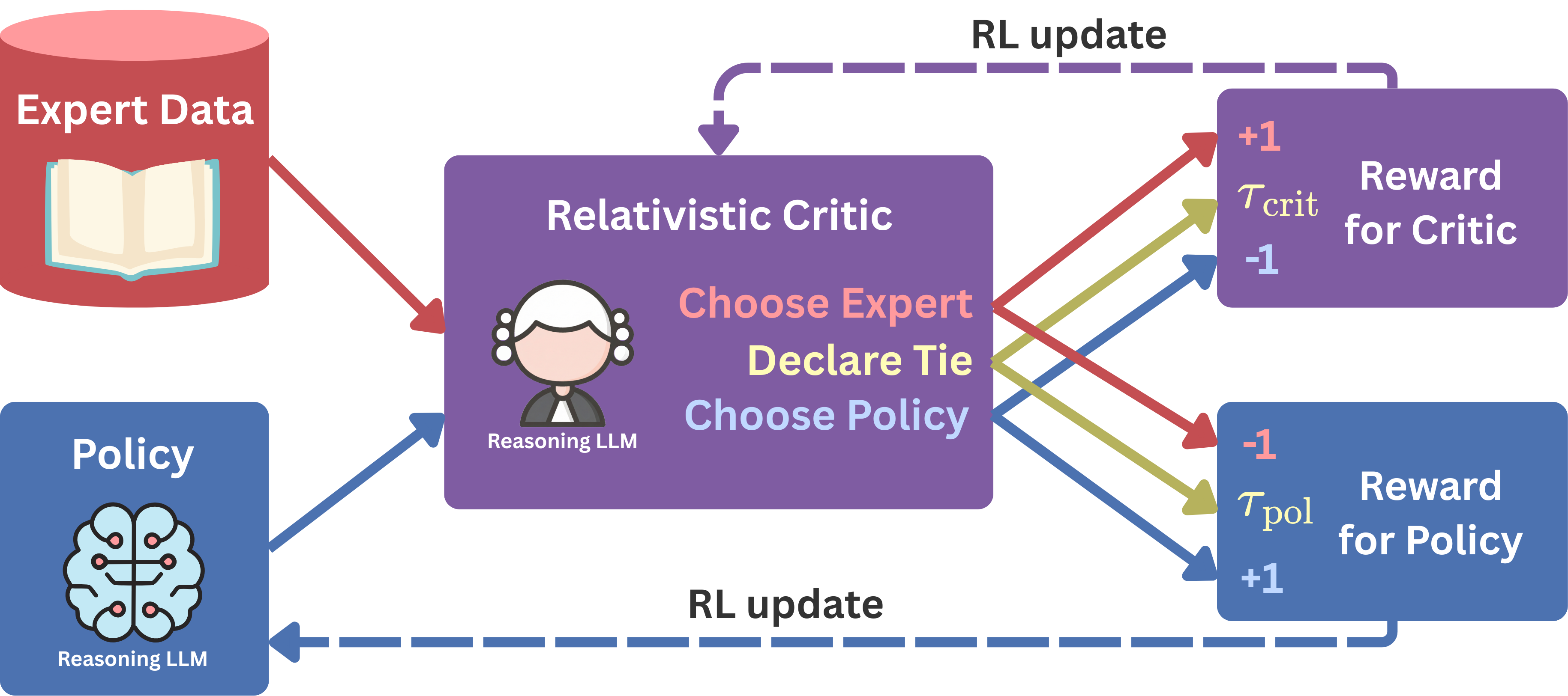
Figure 1: Overview of RARO. The framework creates an adversarial game between a policy and a relativistic critic. The policy generates an answer given a question, while the critic learns to distinguish between the policy’s answer and an expert’s answer for the same question. The critic is rewarded for correctly identifying the expert answer, while the policy is rewarded for deceiving the critic. Additionally, the critic can declare a tie, yielding tie rewards for both the policy and the critic. Both the policy and the critic are trained jointly and continuously via RL.

2 Related Work

2.1 Reinforcement Learning with Verifiable Rewards

Chain-of-Thought (CoT) prompting (wei2022chain) is a simple yet effective technique that enables LLMs to generate intermediate reasoning tokens, steering them toward correct answers. This approach has become a central focus for enhancing reasoning, pairing naturally with test-time scaling for further performance gains (snell2024scalingllmtesttimecompute).

Currently, the standard method to elicit such strong CoT capabilities is Reinforcement Learning with Verifiable Rewards (RLVR). RLVR methods train LLMs to produce long reasoning traces on tasks with ground-truth verifiers, enabling recent open-source models to achieve expert-level performance (deepseek-r1; yang2025qwen3technicalreport).

The dominant algorithm in this space is Group Relative Policy Optimization (GRPO) (grpo-deepseekmath), which builds upon Proximal Policy Optimization (PPO) (ppo) by estimating advantages via group-wise sample averages. Subsequent works like DAPO (yu2025dapoopensourcellmreinforcement) and GSPO (gspo) have further improved its efficiency and stability. However, while RLVR is highly effective, it is fundamentally constrained to verifiable tasks such as mathematics and competitive programming.

2.2 General Reasoning Learning

While RLVR is effective for training LLMs to reason on readily verifiable tasks, it does not directly extend to the broader setting of learning reasoning on real-world domains with no verifiers, yet many of these tasks could still benefit from explicit reasoning  (zhou2025verifree).

Although no consensus method exists for general reasoning learning to our knowledge, several recent efforts make early progress. zhou2025verifree and gurung2025learningreasonlongformstory propose to train LLMs to reason with reward derived from the model’s own logits on expert answers rather than from an external verifier. jia2025writingzerobridgegapnonverifiable propose a pairwise generative reward model with a PPO-style objective for non-verifiable writing tasks, achieving gains without external training signals. gunjal2025rubricsrewardsreinforcementlearning propose using an LLM-as-judge (gu2025surveyllmasajudge) together with pre-generated rubrics from strong LLM to provide rewards for non-verifiable tasks. ma2025generalreasoneradvancingllmreasoning distill a model-based verifier from a strong teacher to train general reasoners without rule-based verifiers. li2025internbootcamptechnicalreportboosting investigate large-scale multi-task RLVR, hypothesizing that breadth across many tasks induces stronger general reasoning. We build on this line of work while adopting a demonstration-only setting and a complementary perspective based on Inverse Reinforcement Learning.

2.3 Inverse Reinforcement Learning

Inverse Reinforcement Learning (IRL) (ng2000algorithms) studies the task of recovering a reward function for which an observed expert policy is near-optimal. A seminal application is robust imitation learning, most notably Generative Adversarial Imitation Learning (GAIL) (ho2016generativeadversarialimitationlearning), casting imitation as an adversarial game between a policy and a discriminator.

sun2025inverserlignmentlargelanguagemodel recently investigated the application of IRL for aligning LLMs with expert demonstrations. They show that a classifier trained in the IRL paradigm can serve as an effective reward model for Best-of-N sampling. However, their work stops short of exploring stable, joint adversarial training, or reasoning-intensive tasks, where the model must learn to navigate complex solution spaces rather than aligning with surface-level preferences.

3 Method

We study the general setting where we are given an expert Question–Answer (QA) dataset, and we aim to train a LLM policy to produce expert-level answers via explicit CoT reasoning. We adopt this setting because verifiable tasks are relatively scarce, whereas expert demonstration data are abundant for many non-verifiable domains (e.g., highly upvoted Stack Exchange answers).

To approach this task, we propose a novel inverse reinforcement learning framework that sets up an adversarial interaction between a policy and a relativistic critic: the policy learns to mimic expert answers, while the critic learns to discriminate between policy and expert answers via pairwise comparison. By jointly training both the policy and the critic to reason via RL, we enable the emergence of strong reasoning capabilities from demonstrations alone, without requiring task-specific verifiers.

3.1 From Maximum Likelihood to Reward Gradient

Setup.

Let $D=\{(q_{i},a_{i})\}_{i=1}^{n}$ denote the expert QA dataset. We parameterize our LLM policy as a conditional latent-variable model (trice) $\pi_{\theta}(a,z\mid q)$, a distribution over answers $a$ and CoT reasonings $z$ conditioned on a question $q$. We let $\hat{p}_{q}(\cdot)$ denote the empirical distribution of questions in $D$, $\hat{p}_{a\mid q}(\cdot\mid\cdot)$ denote the empirical distribution of expert answers conditioned on a question, and the joint $\hat{p}_{D}=\hat{p}_{a\mid q}\hat{p}_{q}$ denote the empirical distribution of dataset pairs $(q,a)$.

A natural baseline for producing expert-quality answers is the maximum likelihood (ML) objective on expert demonstrations: $\arg\max_{\theta}\;\mathbb{E}_{(q,a)\sim\hat{p}_{D}}\!\left[\log\pi_{\theta}(a\mid q)\right]$.

However, for models that perform CoT reasoning before producing an answer, each $(q,a)$ is associated with many possible CoT traces. Thus, the marginal likelihood required by the ML objective, $\pi_{\theta}(a\mid q)=\sum_{z}\pi_{\theta}(a,z\mid q)$, involves summing over a combinatorially large (often effectively unbounded) set of traces, rendering exact computation and its gradients computationally impractical.

Inverse Reinforcement Learning.

To address this intractability, we adopt the perspective of Inverse Reinforcement Learning (IRL). Rather than maximizing the marginal likelihood directly, we learn a parameterized reward $r_{\phi}(a,q)$ over QA pairs such that optimizing a policy $\pi_{\theta}(a\mid q)$ with respect to $r_{\phi}$ yields a “near-optimal” policy that approximately maximizes the ML objective.

We formalize “near-optimality” via the KL-regularized reward-maximization objective. Under this objective, it can be shown (awr) that the optimal policy has the following closed-form solution:

$$\pi_{\theta^{\star}(\phi)}(a\mid q)=\frac{1}{Z_{\theta^{\star}(\phi)}(q)}\,\pi_{\mathrm{ref}}(a\mid q)\,\exp\!\Bigg\{\frac{1}{\beta}\,r_{\phi}(a,q)\Bigg\},$$

where $Z_{\theta^{\star}(\phi)}(q)$ is the partition function, $\pi_{\mathrm{ref}}$ is a fixed reference policy, and $\beta>0$ controls the strength of the KL-regularization. See Appendix A.1 for the proof.

Reward Gradient.

With the closed-form expression for the optimal policy under the reward model $r_{\phi}$, we can derive the corresponding gradient needed to optimize it by differentiating the negative ML loss with respect to $\phi$:

$$\nabla_{\phi}\mathcal{L}(\phi)=\frac{1}{\beta}\Big(\underbrace{\mathbb{E}_{(q,a)\sim\hat{p}_{D}}\big[\nabla_{\phi}r_{\phi}(a,q)\big]}_{\text{expert answers}}-\underbrace{\mathbb{E}_{q\sim\hat{p}_{q}}\,\mathbb{E}_{a^{\prime}\sim\pi_{\theta^{\star}(\phi)}(\cdot\mid q)}\big[\nabla_{\phi}r_{\phi}(a^{\prime},q)\big]}_{\text{policy answers}}\Big).$$

See Appendix A.2 for the proof.

Intuition.

The gradient shapes the reward signal by increasing reward model $r_{\phi}(a,q)$ on expert answers and decreasing it on policy answers, thus nudging the policy toward the expert distribution. A concrete algorithm for the alternating optimization is given in Algorithm 4 in Appendix E.

3.2 Reasoning Reward Model

To instantiate this framework, we need to decide on an appropriate architecture for the reward model $r_{\phi}$. Our setting targets difficult QA tasks that benefit from reasoning. Thus, to reliably separate expert from policy answers, we expect the reward model to be at least as capable as the policy.

To this end, we represent $r_{\phi}$ with a reasoning critic $c_{\phi}$ that takes an $(q,a)$ pair and outputs $\ell\in\{\mathrm{expert},\mathrm{policy}\}$, classifying whether an answer is from the expert or the policy. Specifically, we parametrize $r_{\phi}$ as the difference in probabilities of classifying as $\mathrm{expert}$ and $\mathrm{policy}$ for a $(q,a)$ pair.

Under this parameterization, as shown in Appendix A.3, the gradient $\nabla_{\phi}L$ corresponds to the standard policy gradient, and we can further derive an unbiased estimator for $r_{\phi}(a,q)$, resulting in two simple reward functions for the critic and policy.

Reward for Critic:

$$R_{\text{critic}}(\ell,a,q)=\mathbbm{1}_{\ell\text{ is correct}}-\mathbbm{1}_{\ell\text{ is incorrect}}$$

Reward for Policy:

$$R_{\text{policy}}(a,q)=\mathbbm{1}_{\ell=\mathrm{expert}}-\mathbbm{1}_{\ell=\mathrm{policy}},\quad\ell\sim c_{\phi}(\cdot\mid a,q)$$

This allows us to optimize both the critic and policy using GRPO.

Intuition.

Such reward formulation creates an adversarial game between the critic and policy: the critic is rewarded when it correctly classifies answer as coming from the expert or policy, while the policy is rewarded when the critic incorrectly classifies its answer as an expert answer.

Limitations.

Despite the theoreical soundness, this binary classification setup poses challenges for critic learning. As policy approaches the expert, the classification task becomes much more difficult due to a lack of reference answer for the critic to compare against. In addition, with an optimal policy, the critic effectively degenerates to random guessing, providing high-variance, uninformative gradients to the policy, leading to training instability as we observed (see Appendix D.2).

3.3 Relativistic Critic

To address the lack of reference in the binary classification setup, we adopt a relativistic formulation: the critic takes a triplet $(q,a,a^{*})$ consisting of one policy answer and one expert answer, and outputs which is better or tie if they are equal in quality. This resolves the degeneracy where the critic is forced to differentiate even when the policy is optimal. We empirically show that the tie option is crucial for better performance (see Appendix D.2).

Formally, the relativistic critic $c_{\phi}$ takes a question $q$ and two candidate answers $(a^{(1)},a^{(2)})$ and returns a label $\ell\in\{\text{1},\text{2},\text{tie}\}$. Assuming one expert and one policy answer, we can define:

Reward for Critic:

$$R_{\text{critic}}\bigl(q,a^{(1)},a^{(2)}\bigr)=\mathbbm{1}_{\ell\text{ is expert}}+\tau_{\text{crit}}\cdot\mathbbm{1}_{\ell=\text{tie}},\qquad\tau_{\text{crit}}\in[0,1].$$

Reward for Policy:

$$R_{\text{policy}}\bigl(q,a^{(1)},a^{(2)}\bigr)=\mathbbm{1}_{\ell\text{ is policy}}+\tau_{\text{pol}}\cdot\mathbbm{1}_{\ell=\text{tie}},\qquad\tau_{\text{pol}}\in[0,1].$$

where $\tau_{\text{crit}}$ and $\tau_{\text{pol}}$ are tie rewards, new hyperparameters introduced to handle the tie label.

Algorithm 1 Relativistic Critic with KL-Regularized Policy

Inputs: Dataset $D=\{(q_{i},a_{i})\}$; Tie reward $\tau_{\mathrm{pol}},\tau_{\mathrm{crit}}$; Batch $B$; Rollout $K_{\pi},K_{c}$;
Models: Policy $\pi_{\theta}(z,a\mid q)$; Relativistic critic $c_{\phi}(q,a^{(1)},a^{(2)})$.

1:Initialize $\theta,\phi$

2:for $t=1,\dots,T$ do

3:  Draw $\{(q_{i},a^{\mathrm{E}}_{i})\}_{i=1}^{B}\sim D$

4:  for $i=1..B,k=1..K_{\pi}$ do

5:   $\left.\begin{array}[]{@{}p{0.7\linewidth}@{}}$\begin{aligned} &\text{Sample }(z^{\pi}_{i,k},a^{\mathrm{P}}_{i,k})\!\sim\!\pi_{\theta}(z,a\mid q_{i});\text{ build pair }(a^{\mathrm{E}}_{i},a^{\mathrm{P}}_{i,k})\\ &\ell_{i,k}\!\leftarrow\!c_{\phi}(q_{i},a^{\mathrm{E}}_{i},a^{\mathrm{P}}_{i,k})\\ &R^{\mathrm{pol}}_{i,k}\!\leftarrow\!\mathbbm{1}_{\ell\text{ is policy}}+\tau_{\mathrm{pol}}\mathbbm{1}_{\ell=\text{tie}}\end{aligned}$\end{array}\right\}$ Policy rollouts

6:  end for

7:  for $i=1..B,j=1..K_{c}$ do

8:   $\left.\begin{array}[]{@{}p{0.7\linewidth}@{}}$\begin{aligned} &\text{Form pair }(a^{(1)}_{i,j},a^{(2)}_{i,j})\text{ for }q_{i},\text{ query critic }\ell_{i,j}\!\leftarrow\!c_{\phi}(q_{i},a^{(1)}_{i,j},a^{(2)}_{i,j})\\ &R^{\mathrm{crit}}_{i,j}\!\leftarrow\!\mathbbm{1}_{\ell\text{ is expert}}+\tau_{\mathrm{crit}}\mathbbm{1}_{\ell=\text{tie}}\end{aligned}$\end{array}\right\}$ Critic rollouts

9:  end for

10:  GRPO step on $\theta$ to maximize $\mathbb{E}[R^{\mathrm{pol}}_{i,k}]-\beta D_{\mathrm{KL}}(\pi_{\theta}\|\pi_{\mathrm{ref}})$.

11:  GRPO step on $\phi$ to maximize $\mathbb{E}[R^{\mathrm{crit}}_{i,j}]$.

12:end for

13:return $\theta,\phi$

Intuition.

Unlike the binary classification setup, the relativistic critic is now given a pairwise comparison task: the critic is rewarded when it correctly identifies the expert answer, and the policy is rewarded when the critic mistakenly identifies its answer as the expert answer, with additional tie rewards to ensure non-degeneracy and stable learning. Algorithm 1 describes the full training process and see Appendix E for example critic outputs.

3.4 RARO: Relativistic Adversarial Reasoning Optimization

To ensure stable and efficient learning, we implement several optimizations. First, we use a shared LLM for both the critic and the policy, which reduces memory usage and promotes generalization. This allows us to employ data mixing, where policy and critic rollouts are combined in a single batch, simplifying the training loop. To prevent the critic from suffering from catastrophic forgetting, we utilize a replay buffer that mixes past policy rollouts with current ones. Finally, we incorporate several practical improvements to the GRPO algorithm, such as over-length filtering and removing advantage/length normalization. For full implementation details, please refer to Appendix C.1.

Incorporating all of these optimizations into a concrete algorithm, we arrive at our final algorithm, RARO (Relativistic Adversarial Reasoning Optimization), shown in Algorithm 2.

Algorithm 2 RARO (Relativistic Adversarial Reasoning Optimization)

Inputs: Dataset $D=\{(q_{i},a_{i})\}$; Tie reward $\tau_{\mathrm{pol}},\tau_{\mathrm{crit}}$; Loss weight $\lambda_{\mathrm{pol}},\lambda_{\mathrm{crit}}$ Batch $B$; Rollout $K$.
Model: Shared $\theta\to\pi_{\theta},c_{\theta}$. Replay buffer $\mathcal{R}$.

1:Initialize $\theta,\mathcal{R}\leftarrow\emptyset$;

2:for $t=1,\ldots,T$ do

3:  $\mathcal{R}_{\text{new}}\leftarrow\emptyset$

4:  Draw $\{(q_{i},a^{\mathrm{E}}_{i})\}_{i=1}^{B}\sim D$

5:  for $i=1\dots B,\,k=1\dots K$ do

6:   $\left.\begin{array}[]{@{}p{0.7\linewidth}@{}}$\begin{aligned} &(z^{\mathrm{P}}_{i,k},a^{\mathrm{P}}_{i,k})\sim\pi_{\theta}(\cdot\mid q_{i});\text{ build pair }(a^{\mathrm{E}}_{i},a^{\mathrm{P}}_{i,k})\\ &\ell_{i,k}\sim c_{\theta}(\cdot\mid q_{i},a^{\mathrm{E}}_{i},a^{\mathrm{P}}_{i,k})\\ &R^{\mathrm{pol}}_{i,k}\leftarrow\mathbbm{1}_{\ell_{i,k}\text{ is policy}}+\tau_{\mathrm{pol}}\mathbbm{1}_{\ell_{i,k}=\text{tie}}\\ &\mathcal{R}_{\text{new}}\leftarrow\mathcal{R}_{\text{new}}\cup\{(q_{i},a^{\mathrm{E}}_{i},a^{\mathrm{P}}_{i,k})\}\end{aligned}$\end{array}\right\}$ Policy rollouts

7:  end for

8:  $\mathcal{C}\leftarrow\text{Mix}(\mathcal{R}_{\text{new}},\mathcal{R})$

9:  $\mathcal{R}\leftarrow\mathcal{R}\cup\mathcal{R}_{\text{new}}$

10:  for $(q_{j},a^{\mathrm{E}}_{j},a^{\mathrm{P}}_{j})\in\mathcal{C}$ do

11:   $\left.\begin{array}[]{@{}p{0.7\linewidth}@{}}$\begin{aligned} &\ell_{j}\sim c_{\theta}(\cdot\mid q_{j},a^{\mathrm{E}}_{j},a^{\mathrm{P}}_{j})\\ &R^{\mathrm{crit}}_{j}\leftarrow\mathbbm{1}_{\ell_{j}\text{ is expert}}+\tau_{\mathrm{crit}}\mathbbm{1}_{\ell_{j}=\text{tie}}\end{aligned}$\end{array}\right\}$ Critic rollouts

12:  end for

13:  GRPO step on $\theta$ to maximize: $\lambda_{\mathrm{pol}}J_{\mathrm{pol}}(\theta)+\lambda_{\mathrm{crit}}J_{\mathrm{crit}}(\theta)-\beta D_{\mathrm{KL}}(\pi_{\theta}\|\pi_{\mathrm{ref}})$

14:end for

15:return $\theta$

4 Experimental Setup

4.1 Tasks & Datasets

We evaluate RARO on three diverse reasoning tasks that probe complementary aspects of reasoning. See Appendix C.2 for more details on the datasets.

Countdown.

First, we evaluate our method on the Countdown task, a controlled toy reasoning task where answer verification is much simpler than answer generation. We use a 24-style variant where the goal is to combine four integers to obtain 24 (see Appendix C.2 for details). Through this task, we aim to study the effectiveness of our method on reasoning capabilities in a controlled environment where answer checking is much easier than solution search.

DeepMath.

Then, we evaluate our method on the domain of general math reasoning problems using the DeepMath dataset (he2025deepmath103klargescalechallengingdecontaminated). Compared to Countdown, answer verification in the general math domain is significantly more challenging, often requiring reproduction of the derivation. Through this task, we aim to stress test our method on difficult reasoning environments where verification is as difficult as generation.

Poetry Writing.

Finally, we extend our method to its intended setting of non-verifiable, open-ended reasoning tasks. While there exists benchmarks for non-verifiable domains (arora2025healthbenchevaluatinglargelanguage; paech2024eqbenchemotionalintelligencebenchmark), there is no official training data associated with them. Thus, we choose to evaluate our method and baselines on a custom Poetry Writing dataset. Unlike the math tasks, poetry writing does not admit an objective verifier. Thus, for evaluation, we use GPT-5  (openai2025gpt5) as a judge to evaluate poems in both isolation and in comparison to the expert poem (see Appendix C.2 for details). This task represents the non-verifiable regime that our method aims to handle, where explicit reasoning could significantly improve quality.

4.2 Baselines

We compare RARO against several strong post-training baselines under the same dataset, training, and evaluation setup.

Supervised Fine-Tuning (SFT).

The SFT baseline trains the base models to directly maximizes the conditional log-likelihood of the expert answer given the question, representing the standard use of demonstration data.

Rationalization.

Following prior work on self-rationalizing techniques (zelikman2022starbootstrappingreasoningreasoning), we construct a rationalization baseline that augments each expert answer with an explicit CoT. Concretely, we prompt the base model to annotate the expert demonstrations with free-form rationale, then perform SFT on the concatenated (question, rationale, answer) sequences. This baseline attempts to incentivize the base model to learn to reason before producing the final answer.

Iterative Direct Preference Optimization (DPO).

A natural way to match the policy’s output distribution to the expert is to apply Iterative DPO (rafailov2024directpreferenceoptimizationlanguage). Inspired by Iterative Reasoning Preference Optimization (pang2024iterativereasoningpreferenceoptimization), we perform 3 rounds of DPO iteratively: in each round, we sample one response per question to form preference pairs favoring the expert. We initialize from the SFT checkpoint to mitigate distribution mismatch and report the best performance across rounds.

RL from logit-based reward (RL-Logit).

Recent work has proposed training reasoning LLMs via RL where the reward is derived from the model’s own logits on expert answers rather than from an external verifier (zhou2025verifree; gurung2025learningreasonlongformstory). We implement two variants of such logit-based rewards (see Appendix C.3 for details):

• a log-probability reward, which uses the log-probability of the expert answer $a^{\star}$ given the question $q$ and generated reasoning tokens $z$ as the scalar reward $\log\pi_{\theta}(a^{\star}\mid q,z)$; and

• a perplexity reward, which instead maximizes the negative perplexity of the expert answer under the same conditional distribution.

In our evaluation, we report the metrics from the best performing variant.

RL with Verifiable Reward (RLVR).

For Countdown and DeepMath, where ground-truth verifiers are available, we additionally include a RLVR baseline trained with GRPO on binary rewards given by the verifier. This corresponds to the standard RLVR setting, and serves as an upper-bound for our method on tasks where verification is accessible.

4.3 Training & Evaluation Setup

We evaluate our method and baselines on the Qwen2.5 (qwen2025qwen25technicalreport) family of models, and to focus on improving reasoning performance rather than language understanding, we initialize from the instruction-tuned checkpoints instead of the pretrained model checkpoints. We select the Qwen2.5 family because they are popular non-reasoning LLMs, allowing us to study the effectiveness of our method on eliciting reasoning behaviors in a controlled manner.

Countdown and DeepMath are evaluated with a ground-truth verifier, while Poetry Writing is evaluated with GPT-5 as a judge in two fashions: a scalar score normalized from 1-7 to 0-100 and a win-rate against the expert poem. For both fashions, we prompt GPT-5 to focus its evaluations on prompt adherence and literary qualities. See Appendix C.2 for further details.

Each dataset is split into train, validation, and test sets, and we select our checkpoints based on the highest validation performance. For each dataset and model size, we match dataset splits, rollout budgets, hyperparameters, and sampling configurations when possible to ensure a fair comparison. Unless otherwise specified, all methods are trained and evaluated with a reasoning budget of 2048 tokens. Full implementation details and hyperparameters are provided in Appendix C.

5 Main Results

We present our experimental results structured by task: Countdown, DeepMath, and Poetry Writing. Across these domains, we observe that our method significantly and consistently outperforms all baselines, scaling effectively with both reasoning budget and model size.

5.1 Countdown

Method	Countdown
	accuracy ($\%$) $\uparrow$
RLVR (with verifier)	$57.7\pm 1.6$
Base	$2.0\pm 0.4$
SFT	$40.7\pm 1.6$
Rationalization	$12.5\pm 1.0$
Iterative DPO	$40.4\pm 1.5$
RL-Logit	$2.2\pm 0.4$
RARO	$\mathbf{54.4\pm 1.5}$

Table 1: Main Countdown Results. RARO against baselines at a fixed reasoning budget of 2048 tokens.

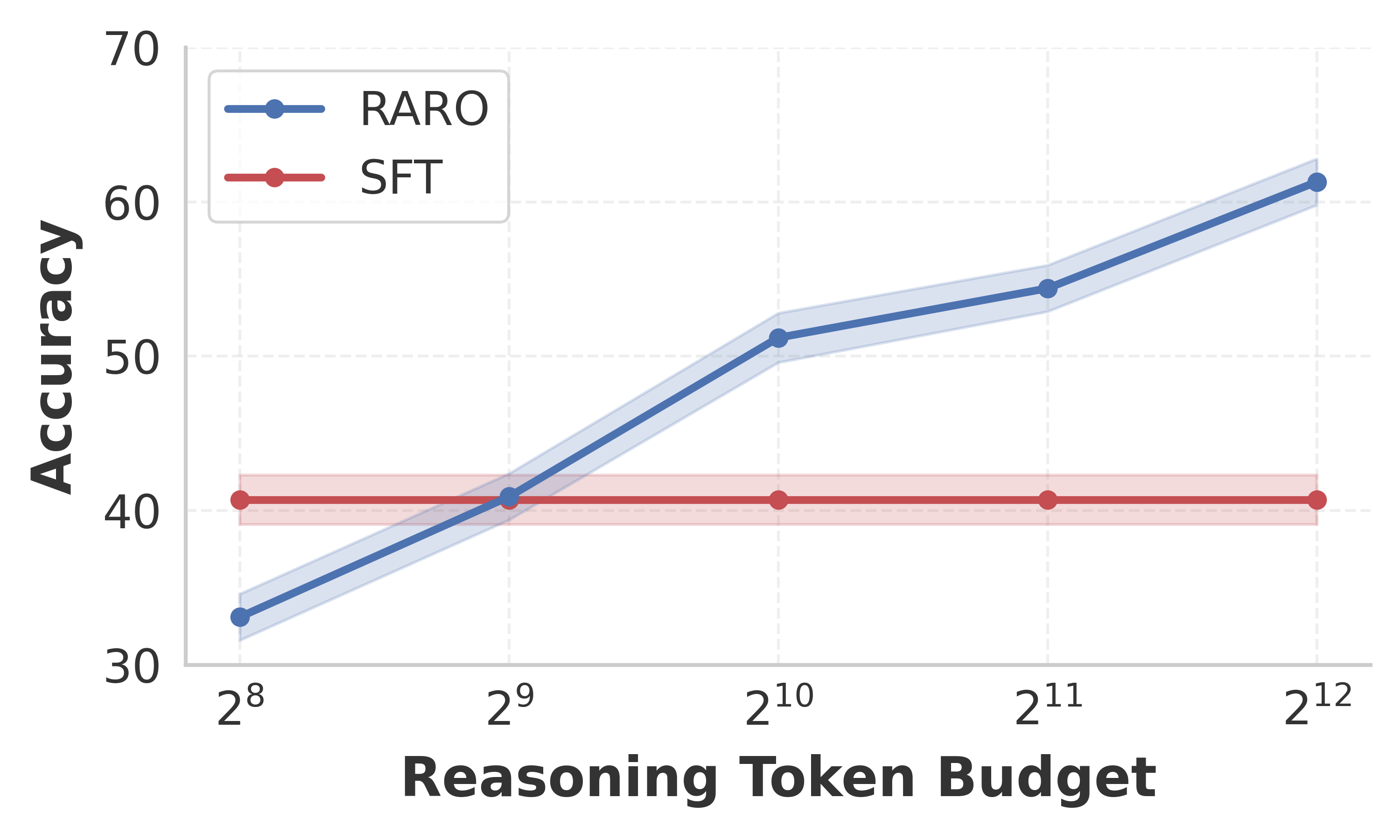
Figure 2: Reasoning Budget Scaling on Countdown. Our method scales effectively with both training and test-time token budget, unlike SFT (best baseline). See Table 7 in Appendix E for detailed data.

We first evaluate RARO on the Countdown task, a controlled toy reasoning task where answer verification is much simpler than answer generation. For this task, we focus our investigation at the 1.5B model size and further ablate our method and baselines with respect to both the training and test-time reasoning token budget. We do not ablate along model size as Countdown is a straightforward task where the reasoning budget is the primary bottleneck rather than model capacity (see Appendix D.1 for additional details).

Superior Performance at Fixed Budget.

At a fixed reasoning budget of 2048 tokens, RARO achieves $54.4\%$ accuracy, significantly outperforming the best verifier-free baseline (SFT, $40.7\%$) by $13.7\%$ and nearly matching the oracle RLVR baseline ($57.7\%$) (Table 1). We also notice that RL-Logit ($2.2\%$) and Rationalization ($12.5\%$) perform rather poorly, and we hypothesize that it is likely due to the base model’s inability to produce high-quality rationalizations or informative logits. The strong performance of RARO demonstrates that our learned critic provides a signal comparable to verification rewards.

Emergence of Self-Correcting Search.

A key qualitative finding is the emergence of explicit search behaviors. As shown in Figure 6, our model learns to explore the solution space dynamically proposing combinations, verifying them, and backtracking when they are incorrect (e.g., “too high”). This self-correction mechanism acts as an internal verifier, allowing the model to recover from errors. Such behavior is absent in the SFT baseline, as it is trained to directly output a candidate answer without any explicit reasoning.

Scaling with Reasoning Budget.

Finally, we examine the scalability of RARO with respect to both training and test-time reasoning token budget. Figure 2 illustrates a clear trend: while the SFT baseline’s performance plateaus at $40.7\%$ regardless of the token budget, our method exhibits continuous improvement as the budget increases, rising from $33.1\%$ at 256 tokens to $61.3\%$ at 4096 tokens. Notably, the result at 4096 tokens is achieved by a model trained with a 2048-token budget, demonstrating that our method can extrapolate to longer reasoning chains at test time without additional training. This scaling behavior confirms that RARO successfully transforms reasoning budget into better performance, a hallmark of effective reasoning.

5.2 DeepMath

Next, we evaluate RARO on the DeepMath dataset, a collection of general math problems. For the DeepMath task, we focus on scaling our method and baselines with respect to model size instead of reasoning budget, as it is a much more difficult setting where model capacity is a real bottleneck in performance.

Method	DeepMath	Poetry	Poetry
	accuracy ($\%$) $\uparrow$	score (0-100) $\uparrow$	win-rate ($\%$) $\uparrow$ (vs. expert)
1.5B
RLVR (with verifier)	$50.9\pm 1.9$	N/A	N/A
Base	$29.6\pm 1.9$	$35.0\pm 0.9$	$0.0\pm 0.0$
SFT	$35.7\pm 1.8$	$53.7\pm 1.0$	$2.3\pm 1.0$
Rationalization	$34.5\pm 2.0$	$35.6\pm 1.6$	$0.8\pm 0.5$
Iterative DPO	$33.0\pm 1.9$	$48.6\pm 0.9$	$0.0\pm 0.0$
RL-Logit	$37.7\pm 1.9$	$36.4\pm 0.7$	$0.0\pm 0.0$
RARO	$\mathbf{41.3\pm 1.9}$	$\mathbf{67.8\pm 0.8}$	$\mathbf{7.8\pm 1.7}$
3B
RLVR (with verifier)	$55.8\pm 2.0$	N/A	N/A
Base	$39.4\pm 1.9$	$46.5\pm 0.9$	$0.0\pm 0.0$
SFT	$39.0\pm 1.9$	$57.4\pm 1.0$	$2.3\pm 1.0$
Rationalization	$32.3\pm 1.9$	$30.8\pm 1.9$	$0.4\pm 0.4$
Iterative DPO	$34.2\pm 1.9$	$69.8\pm 0.8$	$6.6\pm 1.5$
RL-Logit	$43.1\pm 2.0$	$46.9\pm 0.8$	$0.4\pm 0.4$
RARO	$\mathbf{49.1\pm 1.9}$	$\mathbf{71.9\pm 0.8}$	$\mathbf{17.2\pm 2.4}$
7B
RLVR (with verifier)	$66.2\pm 1.9$	N/A	N/A
Base	$44.2\pm 2.1$	$54.0\pm 0.9$	$1.2\pm 0.7$
SFT	$42.3\pm 1.9$	$65.4\pm 1.0$	$5.9\pm 1.4$
Rationalization	$48.6\pm 1.9$	$57.7\pm 1.2$	$5.1\pm 1.3$
Iterative DPO	$36.9\pm 2.0$	$66.5\pm 0.9$	$5.1\pm 1.4$
RL-Logit	$49.3\pm 2.0$	$55.4\pm 0.8$	$3.9\pm 1.2$
RARO	$\mathbf{57.5\pm 2.0}$	$\mathbf{77.3\pm 0.8}$	$\mathbf{25.0\pm 2.6}$

Table 2: Main results for DeepMath and Poetry. We report results for RARO against baselines on DeepMath and Poetry Writing across model scales with a reasoning budget of 2048 tokens. For Iterative DPO, we report the max of the 3 rounds. For RL-Logit, we report the best over the 2 variants. See Table 12 in Appendix E for full data.

Significant Improvement over Baselines.

As reported in Table 2, RARO consistently outperforms all verifier-free baselines across model scales. With the 1.5B model, we achieve $41.3\%$ accuracy compared to $37.7\%$ for the best baseline (RL-Logit), an improvement of $3.6\%$. This advantage grows with model size: at 3B, our method ($49.1\%$) surpasses the best baseline (RL-Logit, $43.1\%$) by $6.0\%$, and at 7B, it reaches $57.5\%$, beating it by $8.2\%$. These results demonstrate that our adversarial learning framework provides a strong signal for reasoning that outperforms not only purely supervised approaches like SFT or Rationalization but also RL-Logit.

Stable Training Dynamics.

We further analyze the training dynamics of RARO on DeepMath. As shown in Figure 4 and further in Appendix B, our coupled training objective maintains a robust equilibrium, allowing the policy to steadily improve its reasoning capabilities and response length without collapsing. This stability confirms the robustness of our optimization procedure.

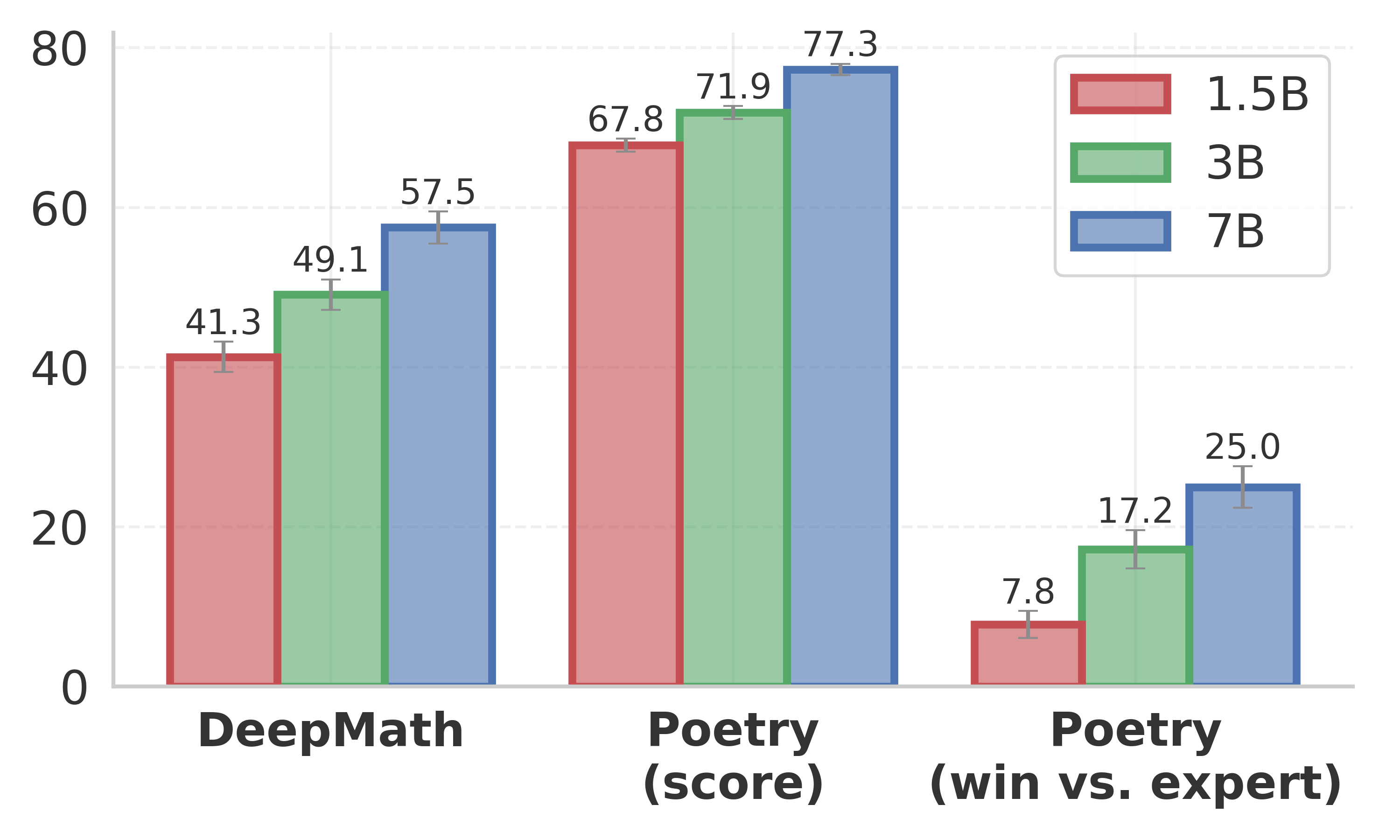
Figure 3: Performance scaling. RARO consistently improves with model size (1.5B to 7B) across both DeepMath and Poetry Writing.

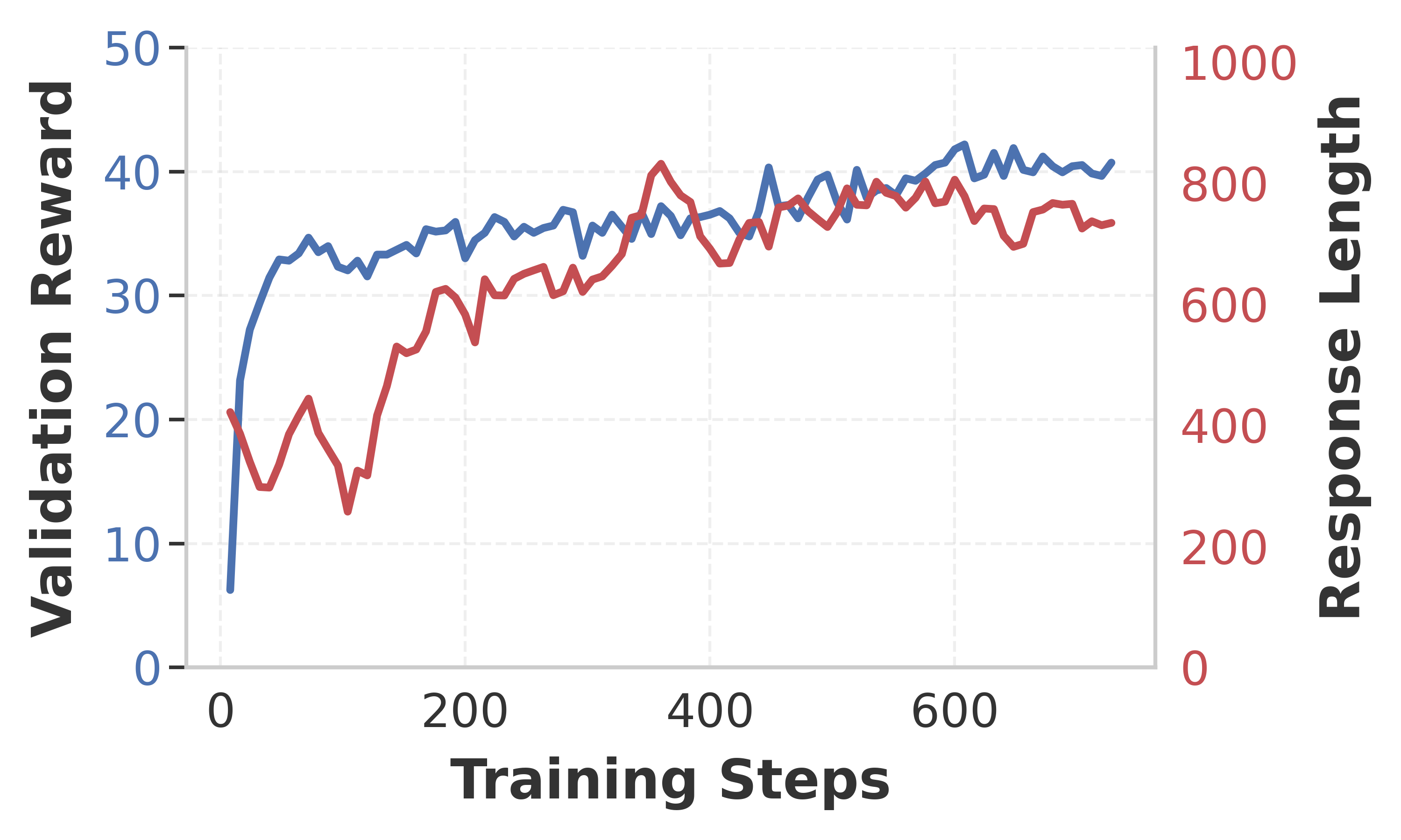
Figure 4: Stable Reward and Length Growth. The validation reward and response length of RARO on DeepMath (1.5B) continuously grows over time, indicating a stable dynamic.

Effective Test-Time Scaling.

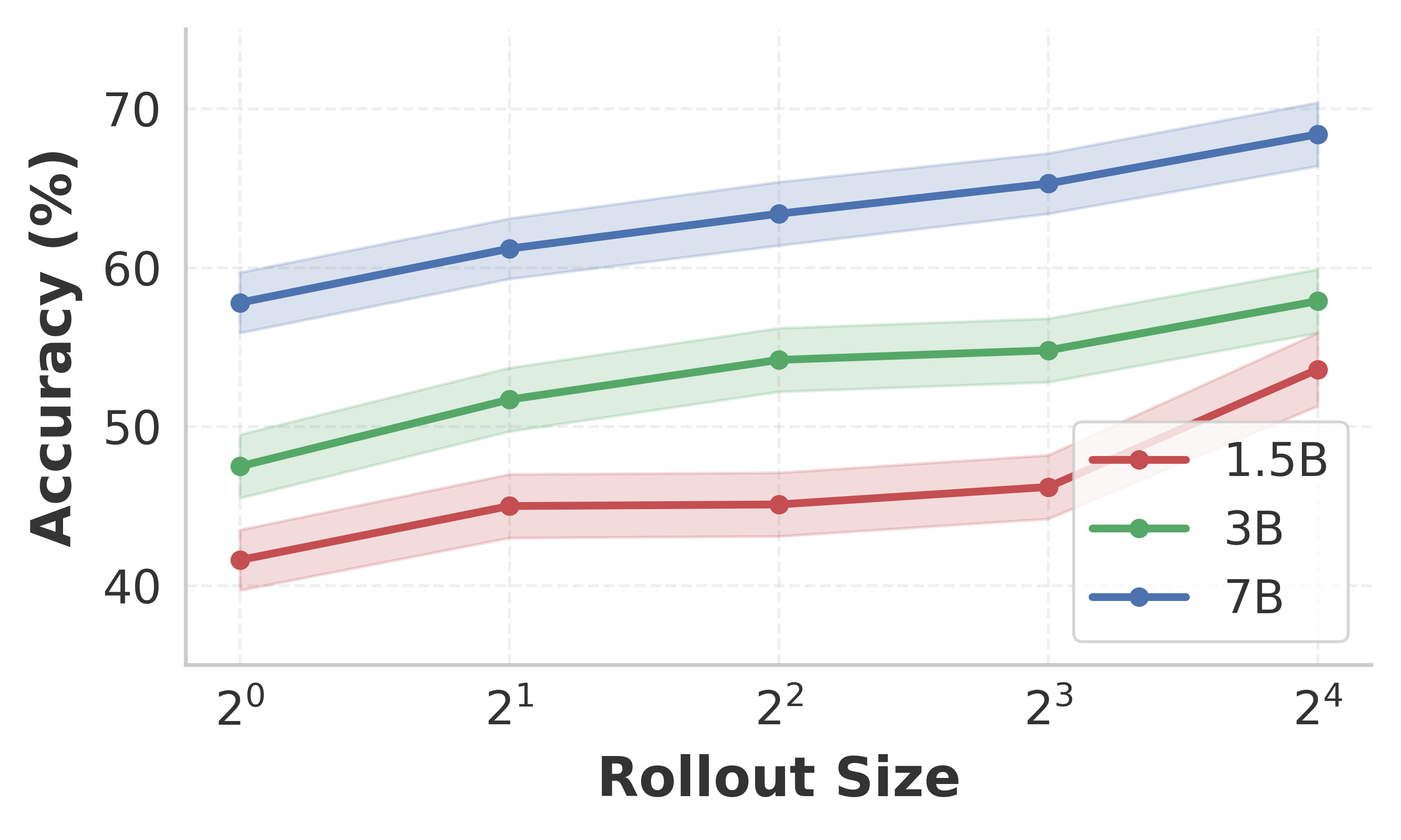
Figure 5: Test-time Scaling (TTS) on DeepMath. Performance improves as the number of rollouts ($N$) increases for all model sizes. See Table 9 in Appendix E for detailed data.

Another key advantage of RARO is that our learned critic enables natural Test-Time Scaling (TTS) to further improve the policy’s performance. Specifically, our critic’s pariwise comparison setup allows for a single-elimination tournament with the critic as the judge (see Algorithm 3), enabling further policy improvements with additional rollouts. As shown in Figure 5 (and detailed in Table 9), increasing the number of rollouts from 1 to 16 consistently improves performance. Notably, with 16 rollouts, RARO achieves $53.6\%$ on the 1.5B model and $57.9\%$ on the 3B model. When comparing against the RLVR baseline with the same TTS strategy (Table 9), we observe that RARO achieves a similar rate of improvement. This result highlights that RARO, when combined with test-time search, can scale effectively, matching the scaling trends of models trained with oracle verifiers.

5.3 Poetry Writing

Finally, we study RARO on Poetry Writing, an open-ended, un-verifiable domain that benefits from specialized reasoning capabilities. For this task, similar to DeepMath, we study RARO across a range of model sizes.

Surpassing Supervised Baselines.

Table 12 reveals a striking performance gap between RARO and baselines. While SFT and Rationalization achieve modest win-rates against expert poetry (peaking at $5.9\%$ with the 7B model), RARO reaches $25.0\%$, a four-fold improvement. This advantage is also reflected in the scoring evaluation, where RARO consistently surpasses baselines (e.g., $67.8$ vs. $53.7$ for SFT at 1.5B). Notably, RL-Logit, leading baseline for DeepMath, fails to produce competitive results, yielding near-zero improvement over the base model ($0.364$ vs. $0.350$ at 1.5B) for both the win-rate and scoring evaluation.

Scaling Creative Capabilities.

A key result is the scalability of RARO with model size in the creative domain. As we increase model capacity from 1.5B to 7B, the win-rate against expert human poems grows substantially, from $7.8\%$ to $25.0\%$. The scoring evaluation similarly improves from $67.8$ to $77.3$. This trend shows that just like verifiable domains, RARO continues to effective scale with model size in open-ended domains.

Figure 6: Qualitative examples for Countdown, DeepMath, and Poetry Writing at 1.5B. For each task, we show the input (top) and the the truncated reasoning and answer sampled from 1.5B models trained with RARO (bottom). See Appendix E for full examples.

Emergent Qualitative Reasoning.

Qualitatively, RARO induces explicit planning and reasoning behaviors even in open-ended domains. As shown in Figure 6 and fully detailed in Figure 18, the model learns to decompose the prompt into key themes (e.g., “disillusionment”, “transience of power”) and stylistic constraints (e.g., “flowing, rhythmic yet contemplative style”) before generating the poem. This demonstrate that RARO effectively elicits reasonings that align the model’s output to creative poems while adhering to the prompt’s nuanced requirements.

6 Conclusion & Future Work

We intoduced RARO (Relativistic Adversarial Reasoning Optimization), a novel approach to training reasoning LLMs using only expert demonstrations, thereby bypassing the need for task-specific verifiers or expensive preference annotations. By formulating the problem as Inverse Reinforcement Learning and incorporating a relativistic critic setup, we obtain a principled and stable adversarial training algorithm that yields strong reasoning capabilities.

Our experiments demonstrate the effectiveness of RARO: (i) on the controlled Countdown task, it not only outperforms verifier-free baselines but also nearly matches the performance of RLVR; (ii) on the general math domain, it exhibits similar desirable scalability trends to RLVR while outperforming baselines without verification; and (iii) on the open-ended Poetry Writing task, it successfully elicits emerging specialized reasoning capabilities and significantly surpasses all baselines. Together, these findings suggest that RARO is a promising and practical approach for training reasoning models without reliance on explicit verifiers.

Future work includes: (i) extending the framework to more generalized adversarial setups that stabilize training across diverse domains; (ii) improving sample efficiency; (iii) scaling the method to larger, state-of-the-art model sizes; and (iv) developing an alternative critic setup that enables better reward interpretability. See Appendix B for more details.

Appendix A Derivations

A.1 Derivation of Closed-Form Optimal Policy

Proposition A.1.

Consider the KL-regularized reward-maximization objective:

$$\theta^{\star}(\phi)=\arg\max_{\theta}\;\mathbb{E}_{(q,a)\sim\hat{p}_{D}}\Big[r_{\phi}(a,q)-\beta\,D_{\mathrm{KL}}\!\big(\pi_{\theta}(\cdot\mid q)\,\|\,\pi_{\mathrm{ref}}(\cdot\mid q)\big)\Big].$$

The optimal policy has the following closed-form solution:

$$\pi_{\theta^{\star}(\phi)}(a\mid q)=\frac{1}{Z_{\theta^{\star}(\phi)}(q)}\,\pi_{\mathrm{ref}}(a\mid q)\,\exp\!\Bigg\{\frac{1}{\beta}\,r_{\phi}(a,q)\Bigg\},$$

where $Z_{\theta^{\star}(\phi)}(q)$ is the partition function ensuring normalization.

Proof.

We derive the closed-form solution for the KL-regularized reward maximization objective. Consider the objective function for a single question $q$:

$$\mathcal{J}(\pi)=\mathbb{E}_{a\sim\pi(\cdot|q)}\left[r_{\phi}(a,q)\right]-\beta D_{\mathrm{KL}}\big(\pi(\cdot\mid q)\,\|\,\pi_{\mathrm{ref}}(\cdot\mid q)\big).$$ (1)

Expanding the KL divergence term:

$$D_{\mathrm{KL}}(\pi\|\pi_{\mathrm{ref}}) =\mathbb{E}_{a\sim\pi(\cdot|q)}\left[\log\frac{\pi(a\mid q)}{\pi_{\mathrm{ref}}(a\mid q)}\right]$$

$$=\mathbb{E}_{a\sim\pi(\cdot|q)}\left[\log\pi(a\mid q)-\log\pi_{\mathrm{ref}}(a\mid q)\right].$$

Substituting this back into the objective:

$$\mathcal{J}(\pi) =\mathbb{E}_{a\sim\pi(\cdot|q)}\left[r_{\phi}(a,q)-\beta\log\pi(a\mid q)+\beta\log\pi_{\mathrm{ref}}(a\mid q)\right]$$

$$=\beta\,\mathbb{E}_{a\sim\pi(\cdot|q)}\left[\frac{1}{\beta}r_{\phi}(a,q)+\log\pi_{\mathrm{ref}}(a\mid q)-\log\pi(a\mid q)\right]$$

$$=-\beta\,\mathbb{E}_{a\sim\pi(\cdot|q)}\left[\log\pi(a\mid q)-\left(\log\pi_{\mathrm{ref}}(a\mid q)+\frac{1}{\beta}r_{\phi}(a,q)\right)\right].$$

Let us define the normalized Gibbs distribution:

$$\pi^{*}(a\mid q)=\frac{1}{Z(q)}\pi_{\mathrm{ref}}(a\mid q)\exp\left(\frac{1}{\beta}r_{\phi}(a,q)\right),$$ (2)

where $Z(q)=\int\pi_{\mathrm{ref}}(a^{\prime}\mid q)\exp\left(\frac{1}{\beta}r_{\phi}(a^{\prime},q)\right)da^{\prime}$ is the partition function. Taking the logarithm of $\pi^{*}$:

$$\log\pi^{*}(a\mid q)=\log\pi_{\mathrm{ref}}(a\mid q)+\frac{1}{\beta}r_{\phi}(a,q)-\log Z(q).$$ (3)

Substituting $\log\pi_{\mathrm{ref}}(a\mid q)+\frac{1}{\beta}r_{\phi}(a,q)=\log\pi^{*}(a\mid q)+\log Z(q)$ into the objective:

$$\mathcal{J}(\pi) =-\beta\,\mathbb{E}_{a\sim\pi(\cdot|q)}\left[\log\pi(a\mid q)-\big(\log\pi^{*}(a\mid q)+\log Z(q)\big)\right]$$

$$=-\beta\left(\mathbb{E}_{a\sim\pi(\cdot|q)}\left[\log\frac{\pi(a\mid q)}{\pi^{*}(a\mid q)}\right]-\log Z(q)\right)$$

$$=-\beta D_{\mathrm{KL}}(\pi\|\pi^{*})+\beta\log Z(q).$$

Since $\beta>0$ and $\log Z(q)$ does not depend on $\pi$, maximizing $\mathcal{J}(\pi)$ is equivalent to minimizing the KL divergence $D_{\mathrm{KL}}(\pi\|\pi^{*})$. By Gibbs’ inequality, $D_{\mathrm{KL}}(\pi\|\pi^{*})\geq 0$, with equality if and only if $\pi=\pi^{*}$ almost everywhere. Thus, the optimal policy is given by:

$$\pi_{\theta^{\star}(\phi)}(a\mid q)=\pi^{*}(a\mid q)=\frac{1}{Z(q)}\pi_{\mathrm{ref}}(a\mid q)\exp\left(\frac{1}{\beta}r_{\phi}(a,q)\right).$$ (4)

∎

A.2 Proof of Reward Gradient

Proposition A.2.

Using the closed-form policy, the gradient of the data log-likelihood $\mathcal{L}(\phi)=\mathbb{E}_{(q,a)\sim\hat{p}_{D}}\!\left[\log\pi_{\theta^{\star}(\phi)}(a\mid q)\right]$ with respect to $\phi$ is:

$$\nabla_{\phi}\mathcal{L}(\phi)=\frac{1}{\beta}\Big(\mathbb{E}_{(q,a)\sim\hat{p}_{D}}\big[\nabla_{\phi}r_{\phi}(a,q)\big]-\mathbb{E}_{q\sim\hat{p}_{q}}\,\mathbb{E}_{a^{\prime}\sim\pi_{\theta^{\star}(\phi)}(\cdot\mid q)}\big[\nabla_{\phi}r_{\phi}(a^{\prime},q)\big]\Big).$$

Proof.

We aim to derive the gradient of the data log-likelihood objective with respect to the reward parameters $\phi$. Recall the objective:

$$\mathcal{L}(\phi)=\mathbb{E}_{(q,a)\sim\hat{p}_{D}}[\log\pi_{\theta^{\star}(\phi)}(a\mid q)].$$ (5)

The optimal policy $\pi_{\theta^{\star}(\phi)}$ takes the closed-form solution:

$$\pi_{\theta^{\star}(\phi)}(a\mid q)=\frac{1}{Z_{\theta^{\star}(\phi)}(q)}\pi_{\mathrm{ref}}(a\mid q)\exp\left(\frac{1}{\beta}r_{\phi}(a,q)\right),$$ (6)

where $Z_{\theta^{\star}(\phi)}(q)=\int\pi_{\mathrm{ref}}(a^{\prime}\mid q)\exp\left(\frac{1}{\beta}r_{\phi}(a^{\prime},q)\right)da^{\prime}$ is the partition function.

Substituting the policy expression into the log-likelihood:

$$\log\pi_{\theta^{\star}(\phi)}(a\mid q) =\log\left(\frac{\pi_{\mathrm{ref}}(a\mid q)\exp\left(\frac{1}{\beta}r_{\phi}(a,q)\right)}{Z_{\theta^{\star}(\phi)}(q)}\right)$$

$$=\log\pi_{\mathrm{ref}}(a\mid q)+\frac{1}{\beta}r_{\phi}(a,q)-\log Z_{\theta^{\star}(\phi)}(q).$$

Since $\pi_{\mathrm{ref}}$ does not depend on $\phi$, the gradient is:

$$\nabla_{\phi}\log\pi_{\theta^{\star}(\phi)}(a\mid q) =\nabla_{\phi}\left(\frac{1}{\beta}r_{\phi}(a,q)-\log Z_{\theta^{\star}(\phi)}(q)\right)$$

$$=\frac{1}{\beta}\nabla_{\phi}r_{\phi}(a,q)-\frac{\nabla_{\phi}Z_{\theta^{\star}(\phi)}(q)}{Z_{\theta^{\star}(\phi)}(q)}.$$

We now compute the gradient of the partition function $Z_{\theta^{\star}(\phi)}(q)$ using the Leibniz integral rule (interchanging gradient and integral):

$$\nabla_{\phi}Z_{\theta^{\star}(\phi)}(q) =\nabla_{\phi}\int\pi_{\mathrm{ref}}(a^{\prime}\mid q)\exp\left(\frac{1}{\beta}r_{\phi}(a^{\prime},q)\right)da^{\prime}$$

$$=\int\pi_{\mathrm{ref}}(a^{\prime}\mid q)\nabla_{\phi}\exp\left(\frac{1}{\beta}r_{\phi}(a^{\prime},q)\right)da^{\prime}$$

$$=\int\pi_{\mathrm{ref}}(a^{\prime}\mid q)\exp\left(\frac{1}{\beta}r_{\phi}(a^{\prime},q)\right)\left(\frac{1}{\beta}\nabla_{\phi}r_{\phi}(a^{\prime},q)\right)da^{\prime}.$$

Substituting this back into the gradient term for $\log Z_{\theta^{\star}(\phi)}(q)$:

$$\frac{\nabla_{\phi}Z_{\theta^{\star}(\phi)}(q)}{Z_{\theta^{\star}(\phi)}(q)} =\int\frac{\pi_{\mathrm{ref}}(a^{\prime}\mid q)\exp\left(\frac{1}{\beta}r_{\phi}(a^{\prime},q)\right)}{Z_{\theta^{\star}(\phi)}(q)}\left(\frac{1}{\beta}\nabla_{\phi}r_{\phi}(a^{\prime},q)\right)da^{\prime}$$

$$=\int\pi_{\theta^{\star}(\phi)}(a^{\prime}\mid q)\left(\frac{1}{\beta}\nabla_{\phi}r_{\phi}(a^{\prime},q)\right)da^{\prime}$$

$$=\mathbb{E}_{a^{\prime}\sim\pi_{\theta^{\star}(\phi)}(\cdot\mid q)}\left[\frac{1}{\beta}\nabla_{\phi}r_{\phi}(a^{\prime},q)\right].$$

Finally, averaging over the dataset $(q,a)\sim\hat{p}_{D}$:

$$\nabla_{\phi}\mathcal{L}(\phi) =\mathbb{E}_{(q,a)\sim\hat{p}_{D}}\left[\frac{1}{\beta}\nabla_{\phi}r_{\phi}(a,q)-\mathbb{E}_{a^{\prime}\sim\pi_{\theta^{\star}(\phi)}(\cdot\mid q)}\left[\frac{1}{\beta}\nabla_{\phi}r_{\phi}(a^{\prime},q)\right]\right]$$

$$=\frac{1}{\beta}\left(\mathbb{E}_{(q,a)\sim\hat{p}_{D}}[\nabla_{\phi}r_{\phi}(a,q)]-\mathbb{E}_{q\sim\hat{p}_{q}}\mathbb{E}_{a^{\prime}\sim\pi_{\theta^{\star}(\phi)}(\cdot\mid q)}[\nabla_{\phi}r_{\phi}(a^{\prime},q)]\right).$$

This completes the derivation. ∎

A.3 Derivation of Reasoning Reward Gradient

Proposition A.3.

Let the reward be parameterized by a critic $c_{\phi}(\ell\mid a,q)$ with labels $\ell\in\{\mathrm{expert},\mathrm{policy}\}$ as $r_{\phi}(a,q)=c_{\phi}(\ell=\mathrm{expert}\mid a,q)-c_{\phi}(\ell=\mathrm{policy}\mid a,q)$. The gradient of the loss with respect to critic parameters $\phi$ is:

$$\nabla_{\phi}L=\frac{1}{\beta}\,\mathbb{E}_{q\sim\hat{p}_{q}(\cdot)}\!\Bigg[\mathbb{E}_{a\sim\hat{p}_{a\mid q}(\cdot\mid q)\,\cup\,\pi_{\theta}(a\mid q)}\Big[\mathbb{E}_{\ell\sim c_{\phi}(\cdot\mid a,q)}\Big[R(\ell,a,q)\,\nabla_{\phi}\log c_{\phi}(\ell\mid a,q)\Big]\Big]\Bigg],$$

where

$$R(\ell,a,q)=\mathbbm{1}_{\ell\text{ is correct}}-\mathbbm{1}_{\ell\text{ is incorrect}}$$

Proof.

In this section, we derive the specific form of the reward gradient when the reward is parameterized by a critic LLM $c_{\phi}$. Recall from Eq. (A.2) that the gradient of the loss is:

$$\nabla_{\phi}\mathcal{L}(\phi)=\frac{1}{\beta}\left(\mathbb{E}_{(q,a)\sim\hat{p}_{D}}[\nabla_{\phi}r_{\phi}(a,q)]-\mathbb{E}_{q\sim\hat{p}_{q}}\mathbb{E}_{a^{\prime}\sim\pi_{\theta}(\cdot\mid q)}[\nabla_{\phi}r_{\phi}(a^{\prime},q)]\right),$$

where we have approximated the optimal policy $\pi_{\theta^{\star}(\phi)}$ with the current policy $\pi_{\theta}$.

We parameterize the reward using a binary classifier (critic) $c_{\phi}(\ell\mid a,q)$ where $\ell\in\{\mathrm{expert},\mathrm{policy}\}$:

$$r_{\phi}(a,q)=c_{\phi}(\ell=\mathrm{expert}\mid a,q)-c_{\phi}(\ell=\mathrm{policy}\mid a,q).$$

Let $p_{E}=c_{\phi}(\ell=\mathrm{expert}\mid a,q)$ and $p_{P}=c_{\phi}(\ell=\mathrm{policy}\mid a,q)=1-p_{E}$. The gradient of the reward with respect to $\phi$ is:

$$\nabla_{\phi}r_{\phi}(a,q)=2\nabla_{\phi}p_{E}.$$

We can express this gradient using the REINFORCE trick (log-derivative trick) over the binary outcome $\ell$. Consider the quantity:

$$\mathbb{E}_{\ell\sim c_{\phi}(\cdot\mid a,q)}[\tilde{R}(\ell)\nabla_{\phi}\log c_{\phi}(\ell\mid a,q)] =\tilde{R}(\mathrm{expert})p_{E}\nabla_{\phi}\log p_{E}+\tilde{R}(\mathrm{policy})p_{P}\nabla_{\phi}\log p_{P}$$

$$=\tilde{R}(\mathrm{expert})\nabla_{\phi}p_{E}+\tilde{R}(\mathrm{policy})\nabla_{\phi}p_{P}$$

$$=\tilde{R}(\mathrm{expert})\nabla_{\phi}p_{E}+\tilde{R}(\mathrm{policy})(-\nabla_{\phi}p_{E})$$

$$=(\tilde{R}(\mathrm{expert})-\tilde{R}(\mathrm{policy}))\nabla_{\phi}p_{E}.$$

By setting $\tilde{R}(\mathrm{expert})=1$ and $\tilde{R}(\mathrm{policy})=-1$, we obtain:

$$(1-(-1))\nabla_{\phi}p_{E}=2\nabla_{\phi}p_{E}=\nabla_{\phi}r_{\phi}(a,q).$$

Thus, we have the identity:

$$\nabla_{\phi}r_{\phi}(a,q)=\mathbb{E}_{\ell\sim c_{\phi}(\cdot\mid a,q)}\Big[(\mathbbm{1}_{\ell=\mathrm{expert}}-\mathbbm{1}_{\ell=\mathrm{policy}})\nabla_{\phi}\log c_{\phi}(\ell\mid a,q)\Big].$$

Substituting this identity back into the loss gradient expression:

1. Expert Term ($(q,a)\sim\hat{p}_{D}$):

$$\mathbb{E}_{a\sim\hat{p}_{a\mid q}}[\nabla_{\phi}r_{\phi}(a,q)] =\mathbb{E}_{a\sim\hat{p}_{a\mid q}}\Big[\mathbb{E}_{\ell\sim c_{\phi}}\Big[(\mathbbm{1}_{\ell=\mathrm{expert}}-\mathbbm{1}_{\ell=\mathrm{policy}})\nabla_{\phi}\log c_{\phi}(\ell\mid a,q)\Big]\Big].$$

This corresponds to a reward signal of $+1$ when $\ell=\mathrm{expert}$ and $-1$ when $\ell=\mathrm{policy}$.

2. Policy Term ($a\sim\pi_{\theta}$): Note the negative sign in the original gradient formula.

$$-\mathbb{E}_{a\sim\pi_{\theta}}[\nabla_{\phi}r_{\phi}(a,q)] =\mathbb{E}_{a\sim\pi_{\theta}}\Big[-\mathbb{E}_{\ell\sim c_{\phi}}\Big[(\mathbbm{1}_{\ell=\mathrm{expert}}-\mathbbm{1}_{\ell=\mathrm{policy}})\nabla_{\phi}\log c_{\phi}(\ell\mid a,q)\Big]\Big]$$

$$=\mathbb{E}_{a\sim\pi_{\theta}}\Big[\mathbb{E}_{\ell\sim c_{\phi}}\Big[(\mathbbm{1}_{\ell=\mathrm{policy}}-\mathbbm{1}_{\ell=\mathrm{expert}})\nabla_{\phi}\log c_{\phi}(\ell\mid a,q)\Big]\Big].$$

This corresponds to a reward signal of $-1$ when $\ell=\mathrm{expert}$ and $+1$ when $\ell=\mathrm{policy}$.

Combining both terms and grouping the expectations results in the final expression:

$$\nabla_{\phi}L=\frac{1}{\beta}\,\mathbb{E}_{q\sim\hat{p}_{q}}\Bigg[\mathbb{E}_{a\sim\hat{p}_{a\mid q}\cup\pi_{\theta}}\Big[\mathbb{E}_{\ell\sim c_{\phi}}\Big[R(\ell,a,q)\,\nabla_{\phi}\log c_{\phi}(\ell\mid a,q)\Big]\Big]\Bigg],$$

where the reward $R(\ell,a,q)$ aggregates the signs from both cases:

$$R(\ell,a,q)=\mathbbm{1}_{\ell\text{ is correct}}-\mathbbm{1}_{\ell\text{ is incorrect}}$$

This matches the formulation in the method section. ∎

Proposition A.4.

The estimator $\hat{r}_{\phi}(a,q)=\mathbbm{1}_{\ell=\mathrm{expert}}-\mathbbm{1}_{\ell=\mathrm{policy}}$ with $\ell\sim c_{\phi}(\cdot\mid a,q)$ is an unbiased estimator of the reward $r_{\phi}(a,q)=c_{\phi}(\ell=\mathrm{expert}\mid a,q)-c_{\phi}(\ell=\mathrm{policy}\mid a,q)$.

Proof.

We compute the expectation of $\hat{r}_{\phi}(a,q)$ over the sampling distribution $c_{\phi}(\cdot\mid a,q)$:

$$\mathbb{E}_{\ell\sim c_{\phi}(\cdot\mid a,q)}[\hat{r}_{\phi}(a,q)] =c_{\phi}(\ell=\mathrm{expert}\mid a,q)\cdot(1)+c_{\phi}(\ell=\mathrm{policy}\mid a,q)\cdot(-1)$$

$$=c_{\phi}(\ell=\mathrm{expert}\mid a,q)-c_{\phi}(\ell=\mathrm{policy}\mid a,q).$$

Since $c_{\phi}(\ell=\mathrm{policy}\mid a,q)=1-c_{\phi}(\ell=\mathrm{expert}\mid a,q)$, we have:

$$\mathbb{E}[\hat{r}_{\phi}(a,q)]=c_{\phi}(\ell=\mathrm{expert}\mid a,q)-c_{\phi}(\ell=\mathrm{policy}\mid a,q)=r_{\phi}(a,q).$$

∎

Appendix B Future Work

Stability in Long-form Generation.

While RARO exhibits stable training dynamics on verifiable tasks (see Figure 8), we observed some instability in long-form creative tasks. As shown in Figure 7, during training, the policy and critic rewards could oscillate on the Poetry Writing task. Additionally, the validation reward similarly oscillates despite an overall upward trend. This is reminiscent of the instability observed in adversarial training for generative models, where powerful discriminators can overfit to transient artifacts and induce non-stationary learning dynamics for the generator  (karras2020traininggenerativeadversarialnetworks). Future work will focus on developing techniques to stabilize this adversarial game in subjective domains. It will also be important to understand when such oscillations reflect true ambiguity in the task (e.g., multiple equally valid poetic styles) versus undesirable instability that harms downstream user experience.

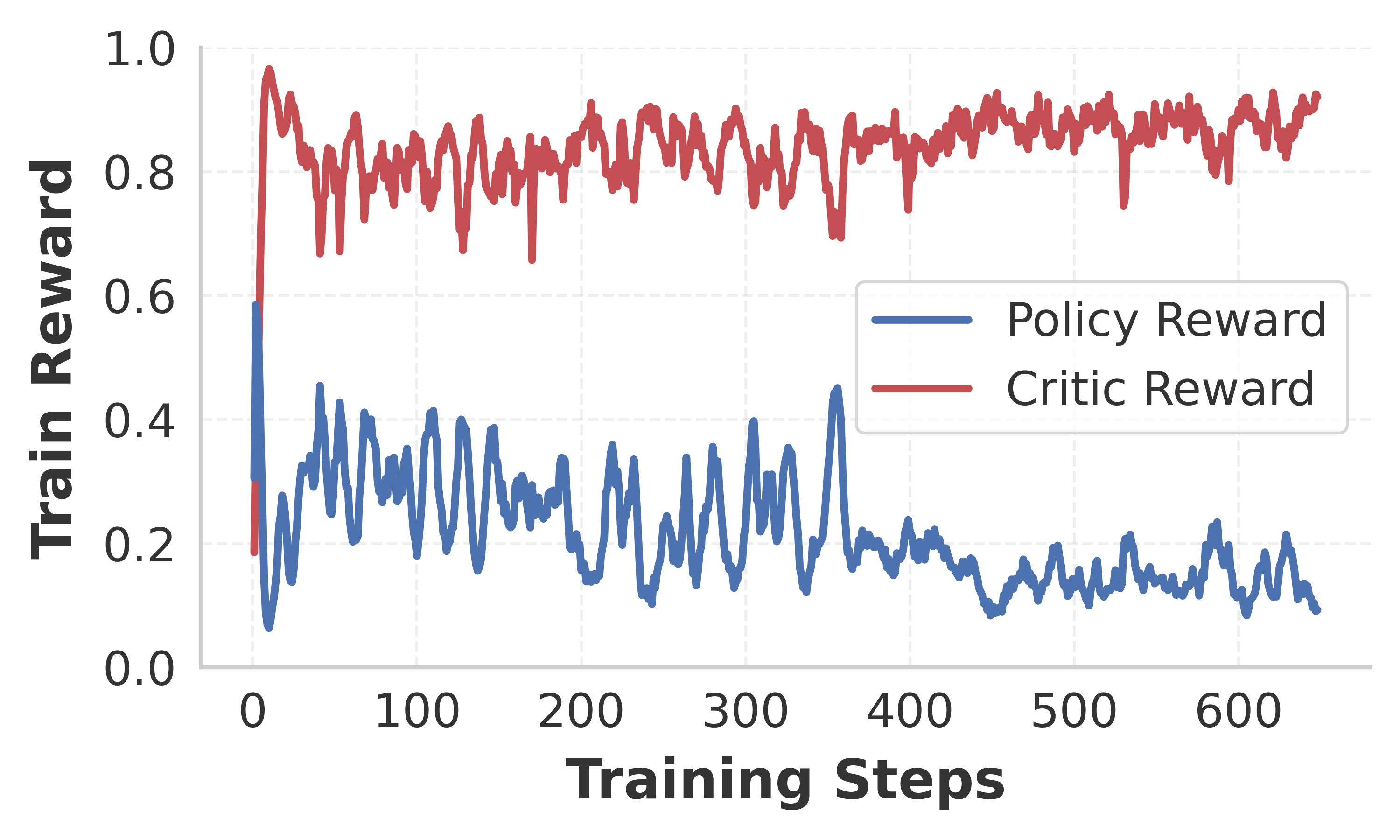
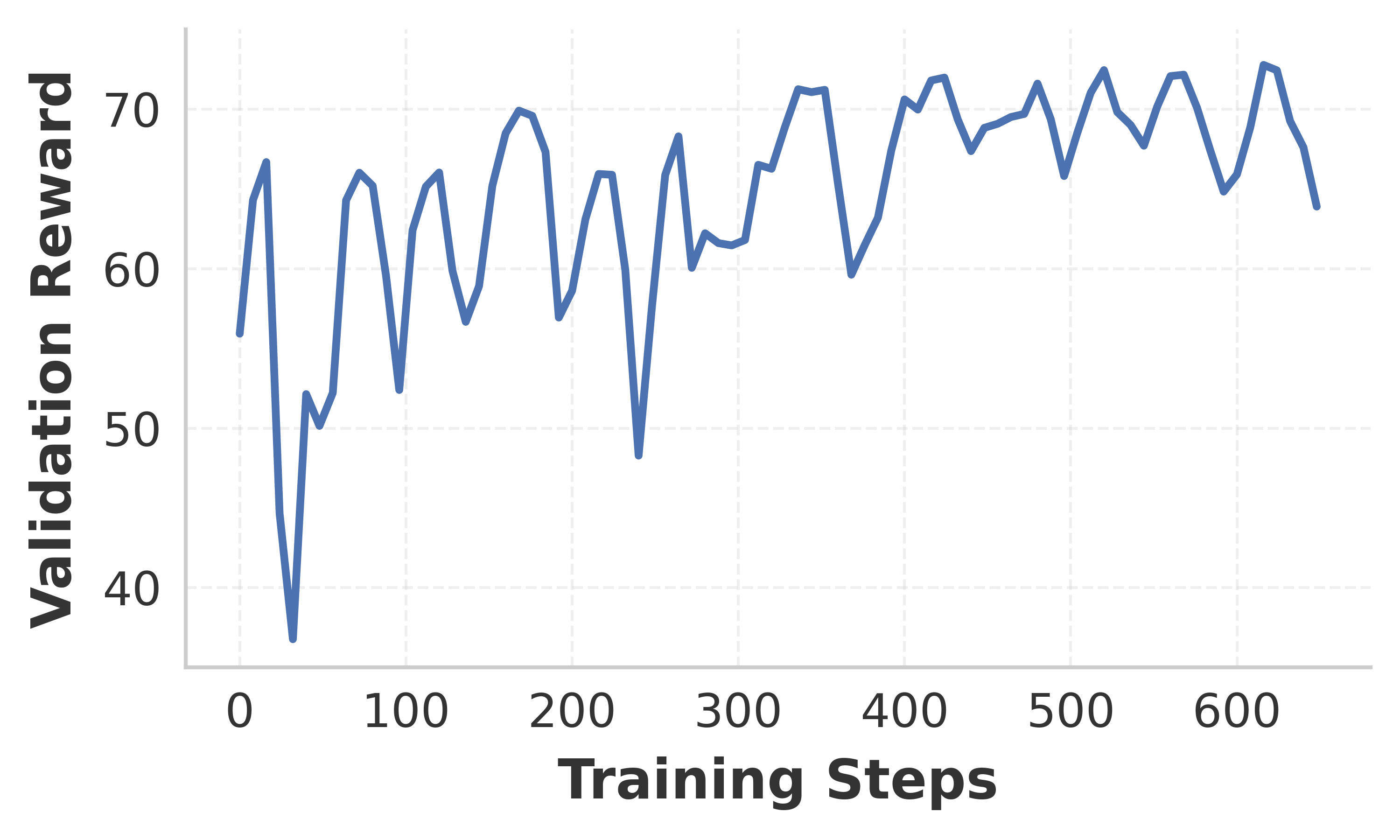
Figure 7: Poetry Writing (7B) Training Dynamics. During training, the policy and critic rewards oscillate on the Poetry Writing task (left). The validation reward similarly oscillates despite an overall upward trend (right).

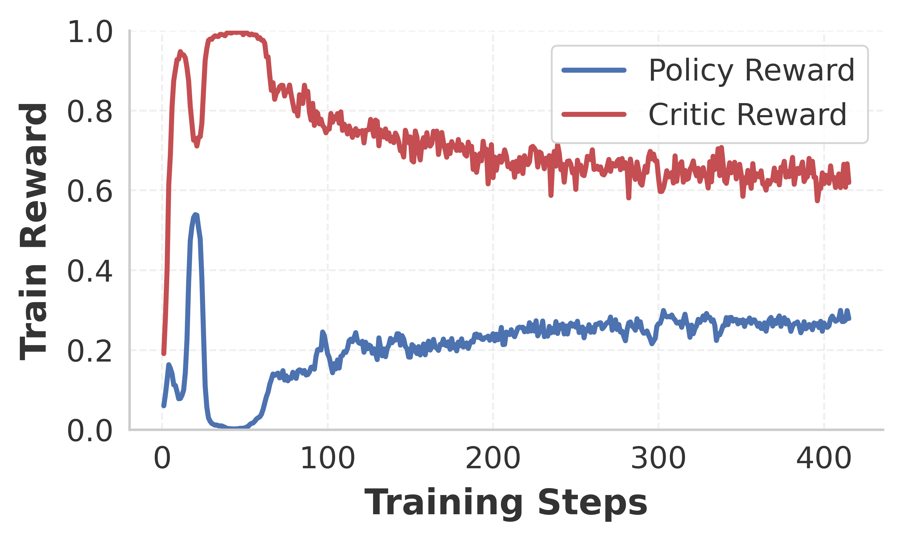
Figure 8: Countdown and DeepMath (1.5B) Training Dynamics. Stable policy and critic rewards during training for Countdown and DeepMath.

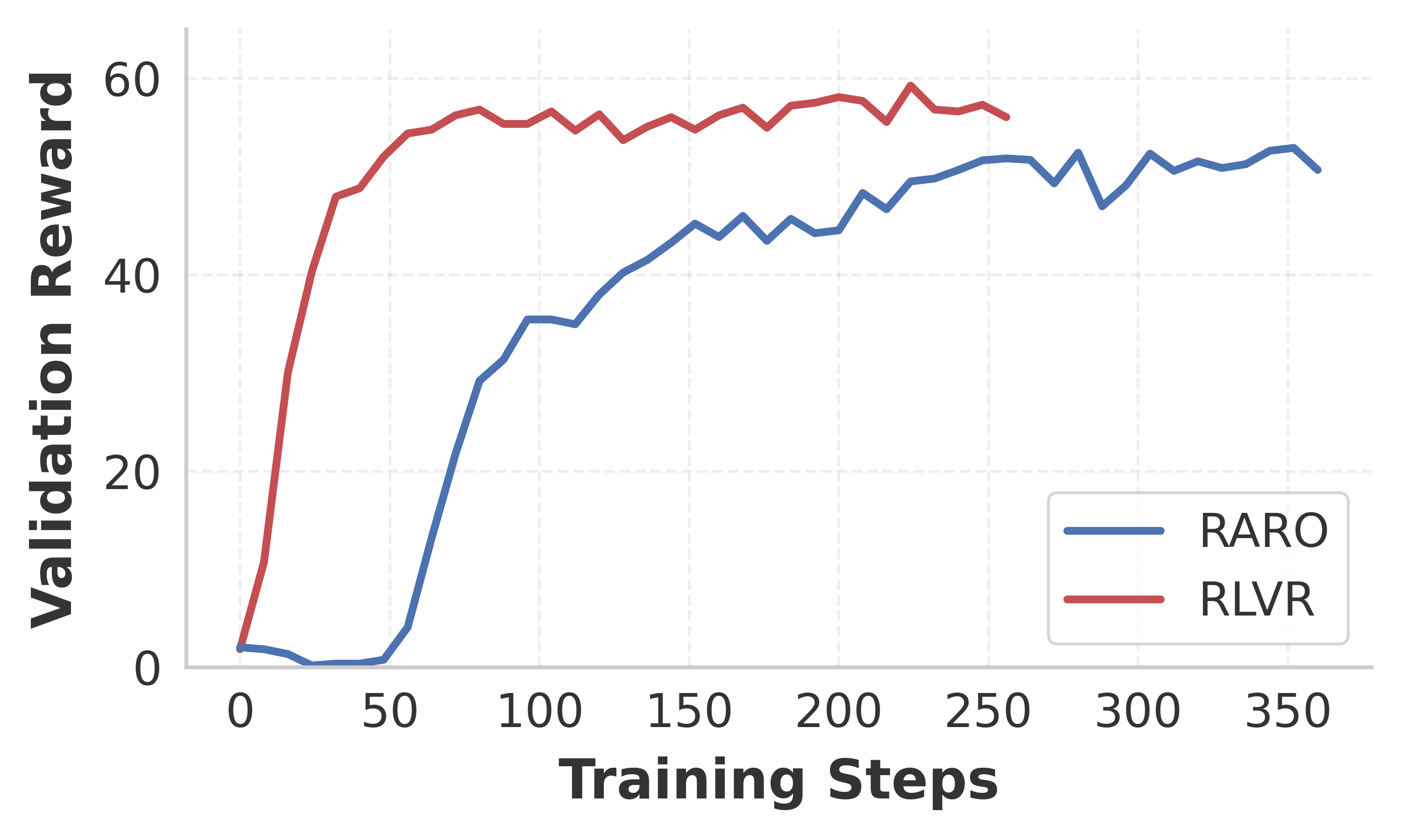
Figure 9: Sample Efficiency Comparison. Under the same hyperparameters, our method is less sample-efficient than RLVR on Countdown.

Sample Efficiency.

While RARO achieves strong final performance, it can be less sample-efficient than RLVR when applied to verifiable tasks. As shown in Figure 9, under identical hyperparameters on the Countdown task, RARO requires more training iterations to reach performance levels comparable to RLVR. This inefficiency stems from the added complexity of jointly training a policy and critic in an adversarial game, where the critic must first learn to discriminate between policy and expert answers before providing a useful training signal. In contrast, RLVR benefits from immediate, oracle feedback. While this gap is unavoidable without access to a ground-truth verifier, future work could explore techniques to accelerate convergence, such as curriculum learning and critic pretraining. A complementary direction is to theoretically characterize the sample complexity of our relativistic adversarial objective and identify conditions under which we can provably bound the sample complexity of RARO.

Reward Interpretability.

One motivation for our critic design is to produce natural-language feedback that resembles human-written explanations. However, even when the critic outputs detailed justifications, it remains challenging to extract a compact, stable, and explicitly human-interpretable rubric that governs its behavior. In practice, the critic’s preferences may be entangled across many latent factors, and at different training steps, the critic may prefer vastly different answers. Making the critic truly interpretable therefore remains an open problem at the intersection of IRL, interpretability, and value learning: promising directions include probing critic representations for concept-like features and distilling the critic into simpler rubric models.

Scaling Reasoning.

We aim to scale RARO to larger base models beyond 7B parameters and beyond reasoning budget of 2048 tokens. Our results already indicate that increasing the reasoning budget—via longer chains of thought at train time and test time—can yield substantial gains. Thus, we are interested in exploring how scaling our method both in model size and reasoning budget can lead to new emerging reasoning capabilities. Another important direction is to finetune models that already exhibit strong reasoning capabilities on new tasks using RARO, so that they can rapidly adapt their reasoning strategies without requiring task-specific verifiers or human preference labels.

Broadening Non-verifiable Domains.

Finally, we plan to apply our approach to a wider range of open-ended domains, such as front-end software development and long-form scientific writing, where expert demonstrations are plentiful online but reliable verifiers are absent. If successful, our approach could enable a new wave of practical LLM applications in these domains, unlocking capabilities where training signals were previously scarce or unreliable. This would allow for the deployment of robust reasoning systems in complex, real-world environments without the need for expensive or impossible-to-design verifiers.

Appendix C Implementation Details

C.1 Stable & Efficient Learning

Here we describe the specific techniques that enable stable and efficient learning in RARO.

Shared LLM for Critic and Policy.

While Algorithm 1 provides a practical procedure for alternating updates of the policy ($\theta$) and the critic model ($\phi$) it requires training two reasoning LLMs and thus incurs long, token-intensive rollouts for both. To reduce memory usage and potentially promote generalization via shared representations, we ultimately use the same underlying LLM to role-play as both the critic and the policy. Our ablations (see Appendix D.2) empirically support that using a shared LLM for the critic and the policy improves performance.

Data Mixing.

In addition, by sharing the same underlying LLM, we can substantially simplify the concrete algorithm by mixing both the critic and policy rollouts in the same batch to compute advantage and loss. This allows us to remove the need for alternating updates between the critic and the policy and instead perform all updates in a single batch. Furthermore, this setup allows us to easily control the “strength” of the policy and the critic by adjusting the weight of the critic and policy loss in the combined objective.

Catastrophic Forgetting & Replay Buffer.

In GAN training (gan), the discriminator often suffers from catastrophic forgetting as the generator “cycles” among modes to fool it (gan-catastrophic-forgetting-mode-collapse; gan-continual-learning). We observe a similar problem in our setting, where policy learns to cycle through a fixed set of strategies to “hack” the critic reward (see Appendix D.2). To mitigate this, we construct half of the critic prompts from a replay buffer of all past policy rollouts, while the other half are sampled from the current batch of policy rollouts, ensuring the critic is continually trained on every mode of “attack” discovered by the policy.

GRPO & Optimizations.

Finally, we address several practical issues when implementing the concrete algorithm. When querying the critic to reward policy rollouts, occasional formatting or networking failures produce invalid rewards; we exclude the affected rollouts from the loss by masking them during backpropagation. Following DAPO (yu2025dapoopensourcellmreinforcement), we also apply over-length filtering: any policy or critic rollout that exceeds a specified token-length threshold is excluded from the objective computation. Finally, inspired by Dr. GRPO (understanding-r1-dr-grpo), we remove advantage normalization and response-length normalization, which we found to introduce bias in our setting.

C.2 Datasets

Countdown.

We use a 24-style variant of the Countdown arithmetic puzzle, where the goal is to combine four integers using basic arithmetic operations to obtain the target value 24. Instances are synthetically generated via an exhaustive search over all possible combination of operands from $[1,50]$ and operations from $\{+,-,\times,\div\}$. The instances are then annotated with expert demonstrations by GPT-5 (openai2025gpt5), discarding instances that GPT-5 cannot solve. The resulting dataset contains 131k total problems, from which we reserve 1024 tasks as a held-out test set. For this task, the final answer is exactly verifiable via a straightforward expression computation, while the underlying search over expressions is substantially more complex.

DeepMath.

To evaluate our method on general math reasoning domain, we use the DeepMath dataset (he2025deepmath103klargescalechallengingdecontaminated), which consists of approximately 103k diverse and high-quality math problems with well-defined ground-truth answers. We utilize the full DeepMath-103K dataset for training and hold out 635 decontaminated problems as a test set. While the dataset provides example reasoning traces beyond ground-truth answers, we discard them in all of our baselines for fairness as our method is not designed to leverage them.

Poetry Writing.

We construct our poetry writing task from a pre-collected corpus of roughly 40k English-language poems sourced from Poetry Foundation . For each poem, we automatically generate a short human-style prompt using GPT-5 and treat the original poem as the expert demonstration. Out of the 40k poems, we reserve 256 poems at random as our test set. Since poetry writing does not admit an objective verifier, we evaluate RARO and baselines using GPT-5. Specifically, we set up two evaluation metrics: scalar score and win-rate. The scalar score is measured by prompting GPT-5 to score the poem on a scale of 1-7 then normalized to 0-100, considering both prompt adherence and literary quality. The win-rate is measured by supplying GPT-5 with both the policy and expert poems and prompting it to determine which poem has higher overall quality.

C.3 Implementation Stack

Supervised methods (SFT and Rationalization).

We train the SFT and Rationalization baselines using Together AI’s managed fine-tuning service. While we monitor the validation loss during training, we ultimately select the checkpoitn for evaluation based on the best validation reward.

Iteractive Direct Preference Optimization (DPO).

Our iterative DPO baselines are implemented using the trl library with PyTorch FSDP2 enabled to support efficient distributed training at all model scales. For evaluation, we similarly select the checkpoint that maximizes the validation reward. We repeat this process for 3 rounds.

RL-based methods (RL-Logit, RLVR, and RARO).

All RL-based methods—RL-Logit, RLVR, and RARO—are implemented on top of the verl framework (verl-sheng2024hybridflow), a flexible and efficient RL framework for LLM post-training. For RLVR, we use the default GRPO implementation in verl without modification, with the reward given by binary ground-truth verifier. For RL-Logit, we extend verl with a custom reward function that computes the scalar reward from the policy logits on expert answers conditioned on the question and generated CoT tokens. To stabilize training and avoid vanishing or exploding rewards, we use two reward variants:

• Log-probability variant: $\max(0.1\times\log\pi_{\theta}(a^{\star}\mid q,z),-1.0)$

• Perplexity variant: $10.0\times\exp(\text{mean}(\log\pi_{\theta}(a^{\star}\mid q,z)))$

For RARO, we further modify the framework to (i) support rewards derived from critic rollouts instead of direct verifiers, and (ii) implement a replay buffer and mixed data pipeline that interleaves policy and critic rollouts for stable joint training of the policy and critic.

Compute setup.

Unless otherwise specified, all non-RL methods (SFT, Rationalization, and DPO) are trained on a single node with 8$\times$H100 GPUs, regardless of model size or reasoning token budget. RL-style methods are more compute intensive: we train RLVR, RL-Logit, and our method on 2 nodes with 8$\times$H100 GPUs each for the 1.5B and 3B models, and on 4 such nodes (32 H100 GPUs in total) for the 7B model.

C.4 Hyperparameters

We summarize the core optimization hyperparameters used for all methods in Tables 3 and 4. Unless otherwise specified, these settings are shared across all tasks (Countdown, DeepMath, and Poetry Writing) and model sizes described in Section 4.

SFT & Rationalization
Hparam Value Epochs $4$ Batch size $8$ Optim AdamW    LR $1\times 10^{-5}$    Weight decay $0.02$    Max grad. norm $1.0$ LR Sched Cosine    Warmup ratio $0.05$    Min LR ratio $0.03$    Num cycles $0.5$

Iteractive DPO
Hparam Value Epochs $1$ Batch size $128$ Optim AdamW    LR $1\times 10^{-6}$    Weight decay 0.01    Max grad. norm 1.0 LR Sched Cosine    Warmup ratio 0.05    Min LR ratio 0.03    Num cycles 0.5 $\beta_{\text{DPO}}$ $0.1$

RLVR & RL-Logit & RARO
Hparam Value Rollout batch $1024$ Rollout temp. $1.0$ Group size $16$ Optim AdamW    LR $1\times 10^{-6}$    Weight decay $0.01$    Max grad. norm $1.0$ Train batch $256$ Clip ratio $[0.2,0.28]$ KL coeff. $10^{-3}$

Table 3: Shared hyperparameters across ours and baselines. SFT and Rationalization share the same AdamW optimizer setup, while DPO uses a different configuration. All three share the same cosine learning-rate schedule. RLVR, RL-Logit, and RARO share the same underlying GRPO setup as described in Section 3.

RARO (Countdown)
Hparam Value $\tau_{\text{pol}}$ $0.6$ $\tau_{\text{crit}}$ $0.55$ $\lambda_{\text{pol}}$ $1/2$ $\lambda_{\text{crit}}$ $1/2$

RARO (DeepMath)
Hparam Value $\tau_{\text{pol}}$ $0.6$ $\tau_{\text{crit}}$ $0.55$ $\lambda_{\text{pol}}$ $1/9$ $\lambda_{\text{crit}}$ $8/9$

RARO (Poetry Writing)
Hparam Value $\tau_{\text{pol}}$ $0.6$ $\tau_{\text{crit}}$ $0.5$ $\lambda_{\text{pol}}$ $1/3$ $\lambda_{\text{crit}}$ $2/3$

Table 4: Hyperparameters for our method. We use the relativistic critic and shared-LLM training setup described in Section 3, with tie rewards $(\tau_{\text{pol}},\tau_{\text{crit}})$ and loss weights $(\lambda_{\text{pol}},\lambda_{\text{crit}})$ chosen to balance exploration and critic supervision for each task.

C.5 Test-Time Scaling Algorithm

Here, we provide additional details for our Test-Time Scaling (TTS) algorithm. As described in Algorithm 3, we implement TTS via a single-elimination tournament. Given a pool of candidate responses $\mathcal{Y}$ generated by the policy, we iteratively pair them and use the learned critic $C_{\phi}$ to select the better response. To mitigate the variance in the critic’s generated reasoning, for each pair of responses $(y_{A},y_{B})$, we sample the critic $K$ times and use a majority vote to determine the winner. We use $K=4$ for all our TTS experiments. Tables 11 and 13 present the full results of RARO with TTS compared to baselines with identical TTS settings.

Algorithm 3 Single-Elimination Tournament for Test-Time Scaling

1:Prompt $x$, Candidates $\mathcal{Y}$, Critic $C_{\phi}$, Votes $K$

2:Best response $y^{*}$

3:while $|\mathcal{Y}|>1$ do

4:  $\mathcal{Y}_{next}\leftarrow\emptyset$

5:  for $i=1$ to $|\mathcal{Y}|$ step 2 do

6:   if $i==|\mathcal{Y}|$ then $\mathcal{Y}_{next}.\text{append}(\mathcal{Y}[i])$; continue

7:   end if

8:   $y_{A},y_{B}\leftarrow\mathcal{Y}[i],\mathcal{Y}[i+1]$

9:   $v_{A}\leftarrow\sum_{k=1}^{K}\mathbb{I}(C_{\phi}(\cdot|x,y_{A},y_{B})\text{ favors }A)$

10:   $\mathcal{Y}_{next}.\text{append}(v_{A}>K/2\ ?\ y_{A}:y_{B})$

11:  end for

12:  $\mathcal{Y}\leftarrow\mathcal{Y}_{next}$

13:end while

14:return $\mathcal{Y}[1]$

Appendix D Additional Results

D.1 Model Size Scaling on Countdown

Method	1.5B	3B
	accuracy ($\%$) $\uparrow$	accuracy ($\%$) $\uparrow$
RLVR	$57.7\pm 1.6$	$53.5\pm 1.6$
RARO	$54.4\pm 1.5$	$49.7\pm 1.6$

Table 5: Model Size Scaling on Countdown.

We systematically study the effect of scaling model size on the performance on Countdown. In addition to the main results at 1.5B reported in Section 5, we conducted additional experiments at 3B. The verifiable baseline, RLVR, exhibits a performance regression, dropping from $57.7\%$ at 1.5B to $53.5\%$ at 3B (Figure 11). Similarly, we observe that the performance of RARO also degrades from $54.4\%$ to $49.7\%$ at 3B. Furthermore, as illustrated in Figure 11, after inital improvements, both RLVR and RARO performance actively decreases as trainiing progresses. While we do not have a definitive explanation, we hypothesize that larger models may be more prone to the training-inference log-probability mismatch problem (yao2025offpolicy), leading to degradation when scaling model capacity. These results indicate that RARO does not inherently contribute to the performance plateau; rather, it is a systematic problem that we observe with RLVR as well.

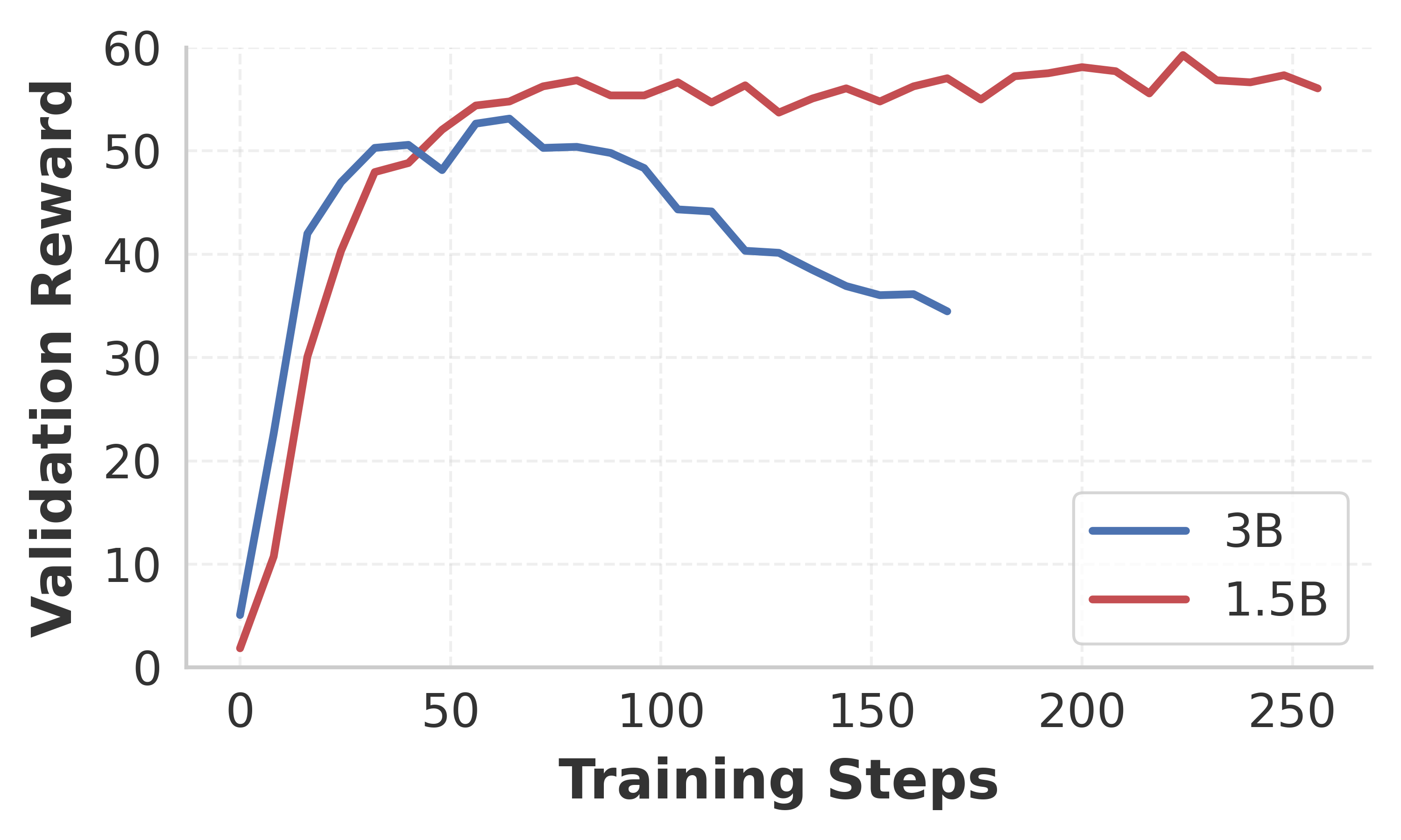
Figure 10: RLVR with a 3B model achieves lower performance than with a 1.5B model.

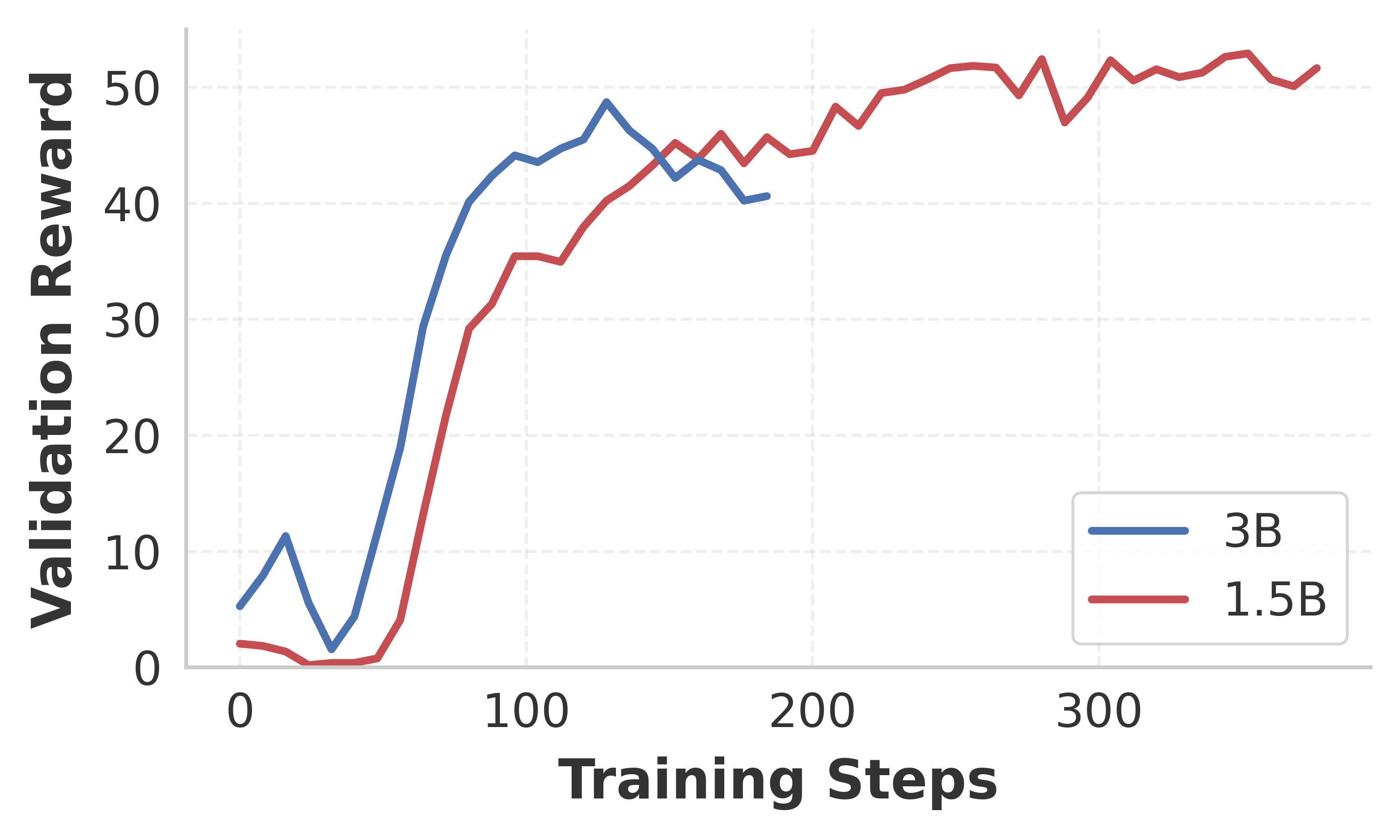
Figure 11: RARO similarly degrades from 1.5B to 3B.

D.2 Ablation Studies

Method	DeepMath 1.5B
	accuracy ($\%$) $\uparrow$
w/o critic reasoning	$35.9\pm 1.9$
w/o relativistic critic	$36.9\pm 1.9$
w/o tie option	$38.6\pm 1.9$
w/o replay buffer	$35.4\pm 1.8$
w/o shared LLM	$39.4\pm 1.9$
RARO	$\mathbf{41.3\pm 1.9}$

Table 6: Ablation results on DeepMath 1.5B. Removing any component leads to performance degradation.

We conduct Leave-One-Out (LOO) ablations on the DeepMath dataset at 1.5B to isolate the contribution of each component in our framework. As summarized in Table 6, removing any single component—the shared LLM, relativistic critic, critic reasoning, tie option, or replay buffer—results in a significant performance degradation compared to our full method ($41.3\%$). This uniform drop confirms that all designed mechanisms are essential for the method’s overall effectiveness.

Beyond aggregate metrics, we observe distinct failure modes associated with particular missing components, illustrated by the training dynamics.

Necessity of Critic Reasoning.

RARO relies on the critic performing explicit CoT reasoning before providing a final judgment. When this reasoning step is removed, the critic loses its capacity to make meaningful distinctions between responses. As shown in Figure 13, instead of providing consistent signals, it collapses into a degenerate state, consistently outputting a tie response regardless of the quality of the policy or expert answer. This failure prevents the policy from receiving useful reward signals, stalling learning.

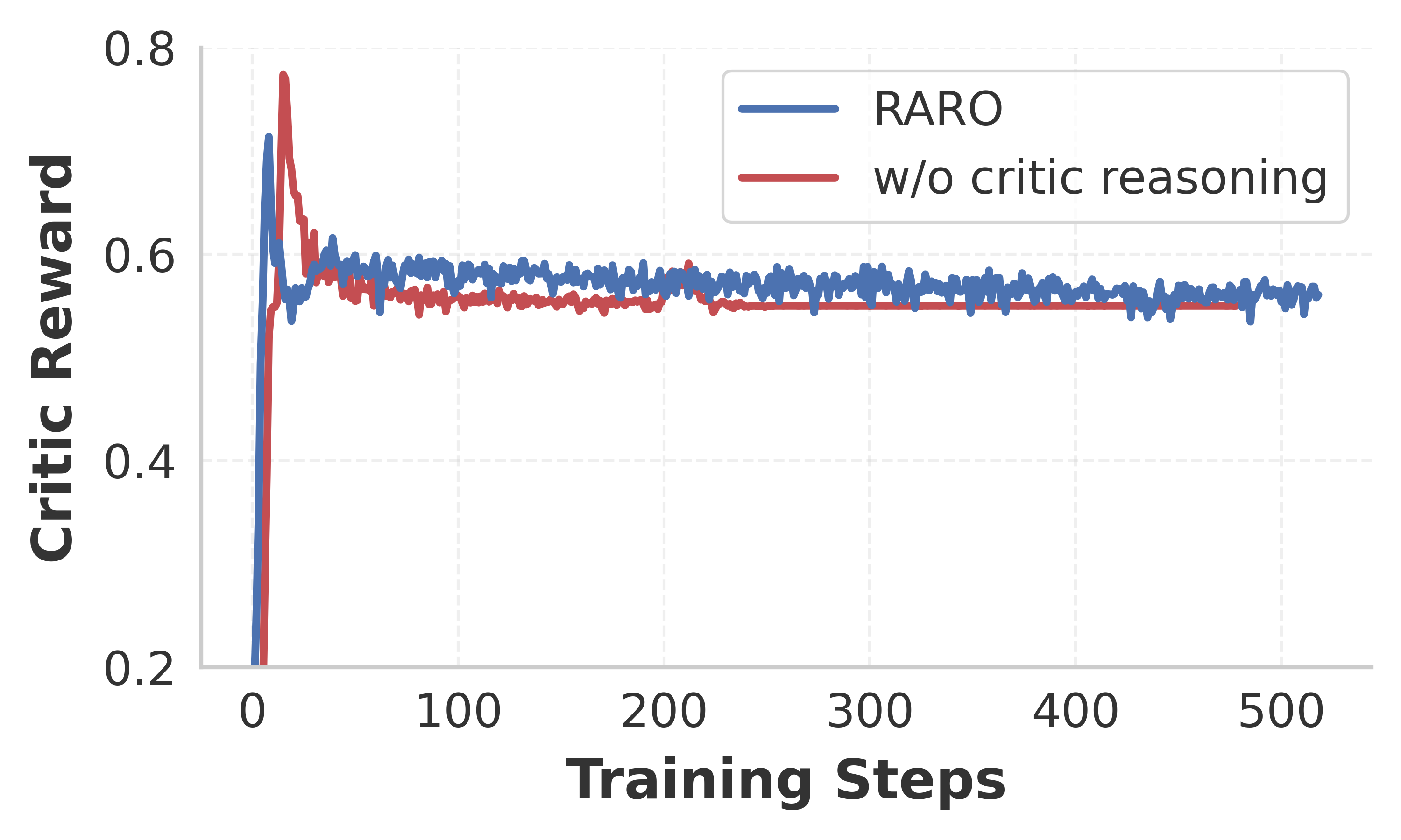
Figure 12: No Critic Reasoning. Without critic reasoning, the critic always outputs tie, preventing the policy from learning.

Figure 13: Tie Distribution. The critic learns to output tie stably for around $70\%$ of the outputs after around 150 training steps.

Importance of Relativistic Setup.

The relativistic critic evaluates the policy’s answer and the expert’s answer in a pairwise fashion rather than in isolation. Without this relativistic setup, the reward signal perceived by the policy exhibits significantly higher variance during training, as illustrated in Figure 15. This instability suggests that the reference answer serves as a crucial anchor enabling stable optimization. We further demonstrate that the critic successfully learns to utilize the tie option defined in our relativistic setup. As shown in Figure 13, the critic learns to output tie stably for around $70\%$ of the outputs after around 150 training steps. In addition, as shown in Table 6, without the tie option, the final policy’s performance drops from $41.3\%$ to $38.6\%$, indicating that the addition of the tie option contributes to the final policy performance.

Role of the Replay Buffer.

Finally, the replay buffer is critical for preventing cycling dynamics. As shown in Figure 15, removing the replay buffer causes the critic’s training reward to oscillate severely after around 300 training steps. This suggests that the policy learns to exploit the critic’s forgetfulness by cycling through adversarial patterns that temporarily fool the critic. This interaction eventually destabilizes the critic completely, leading it to default to a tie output, effectively halting progress.

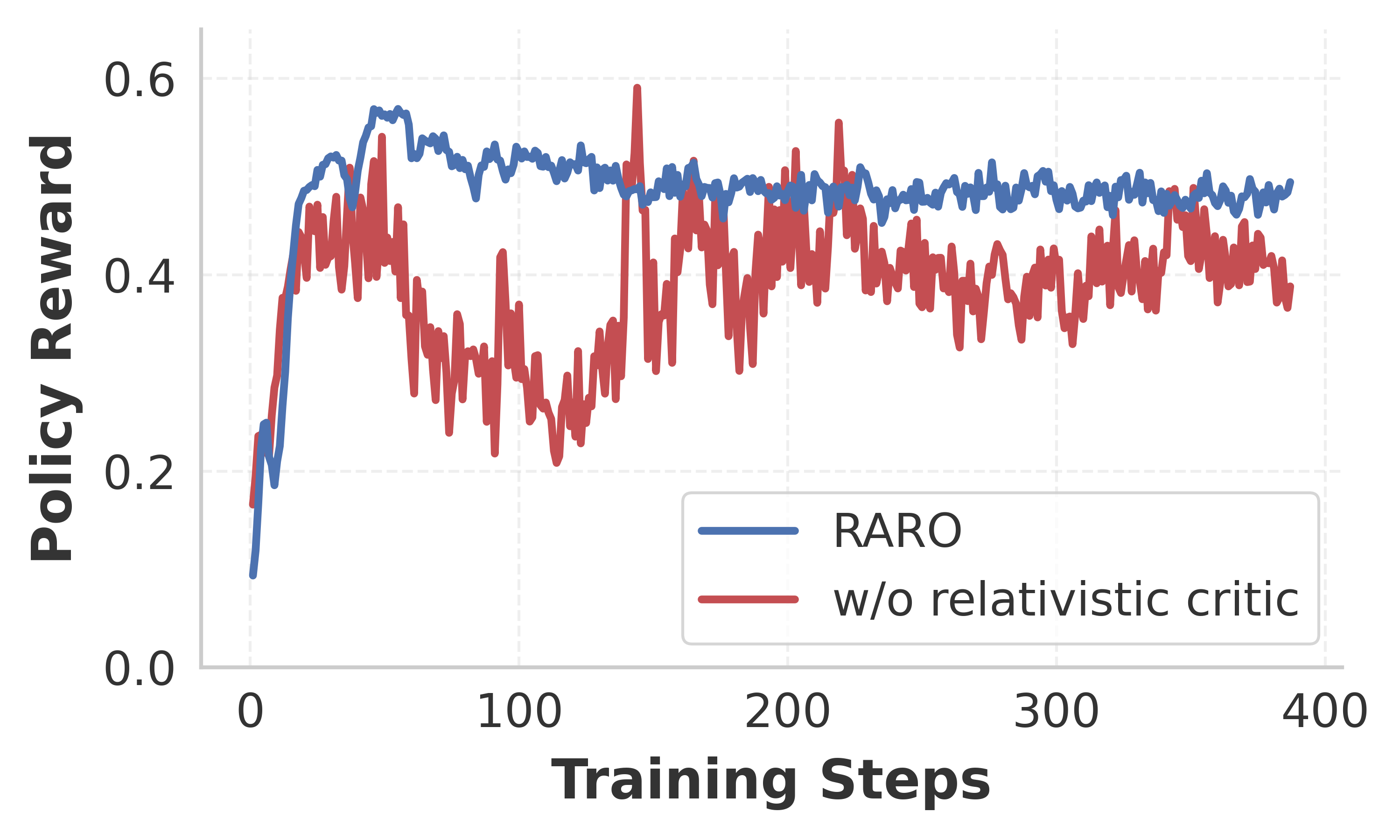
Figure 14: No Relativistic Setup. Without the relativistic setup, the policy reward during training exhibits high variance.

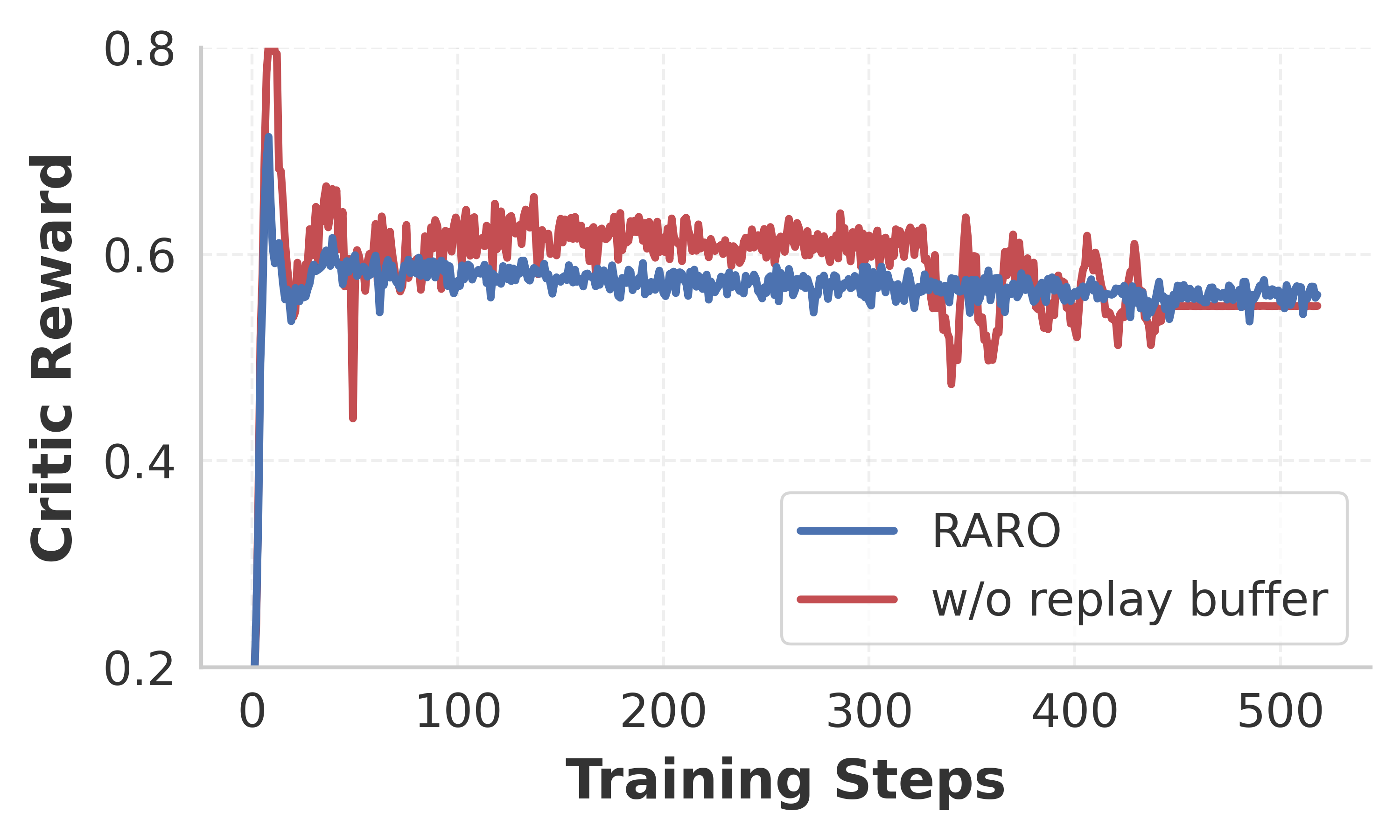
Figure 15: No Replay Buffer. Without a replay buffer, the training suffers from severe oscillations and eventual collapse.

Appendix E Additional Tables & Figures

Budget	256	512	1024	2048	4096
SFT	$40.7\pm 1.6$	$40.7\pm 1.6$	$40.7\pm 1.6$	$40.7\pm 1.6$	$40.7\pm 1.6$
RARO	$33.1\pm 1.5$	$40.9\pm 1.5$	$51.2\pm 1.6$	$54.4\pm 1.5$	$61.3\pm 1.5$

Table 7: Tabular data for Countdown reasoning budget scaling results. Notably, result reported at a budget of 4096 tokens is derived from extrapolating test-time reasoning budget of the model trained at 2048 tokens.

N	1.5B	3B	7B
1	$41.6\pm 1.9$	$47.5\pm 2.0$	$57.8\pm 1.9$
2	$45.0\pm 2.0$	$51.7\pm 2.0$	$61.2\pm 1.9$
4	$45.1\pm 2.0$	$54.2\pm 2.0$	$63.4\pm 2.0$
8	$46.2\pm 2.0$	$54.8\pm 2.0$	$65.3\pm 1.9$
16	$53.6\pm 2.3$	$57.9\pm 2.0$	$68.4\pm 2.0$

Table 8: Tabular data for RARO’s TTS scaling results on DeepMath.

N	1.5B	3B	7B
1	$50.9\pm 1.9$	$55.8\pm 2.0$	$66.2\pm 2.0$
2	$55.5\pm 1.9$	$63.4\pm 1.9$	$68.9\pm 1.9$
4	$59.6\pm 1.9$	$68.6\pm 1.8$	$69.8\pm 1.9$
8	$64.4\pm 1.9$	$72.5\pm 1.7$	$71.5\pm 1.9$
16	$66.1\pm 1.8$	$75.8\pm 1.7$	$76.9\pm 1.9$

Table 9: Tabular data for the RLVR’s TTS scaling results on DeepMath.

Method	Countdown
	accuracy ($\%$) $\uparrow$
RLVR (with verifier)	$57.7\pm 1.6$
Base	$2.0\pm 0.4$
SFT	$40.7\pm 1.6$
Rationalization	$12.5\pm 1.0$
DPO
Round 1	$40.4\pm 1.5$
Round 2	$32.5\pm 1.4$
Round 3	$32.2\pm 1.4$
RL-Logits	$2.2\pm 0.4$
RARO	$\mathbf{54.4\pm 1.5}$

Table 10: Complete results for Countdown at 1.5B.

Method	Countdown
	accuracy ($\%$) $\uparrow$
RLVR (with verifier)	$71.0\pm 1.5$
Base	$4.2\pm 0.6$
SFT	$42.4\pm 1.6$
Rationalization	$11.2\pm 1.0$
DPO
Round 1	$43.1\pm 1.6$
Round 2	$34.8\pm 1.5$
Round 3	$31.6\pm 1.4$
RL-Logits	$3.1\pm 0.5$
RARO	$\mathbf{75.0\pm 1.4}$

Table 11: Complete results for Countdown at 1.5B with TTS.

Algorithm 4 Alternating Reward-Policy Optimization

Inputs: Dataset $D=\{(q_{i},a_{i})\}$; Batch $B$; Learning rates $\eta_{r},\eta_{\pi}$.
Models: Reward $r_{\phi}(a,q)$; Policy $\pi_{\theta}(z,a\mid q)$.

1:Initialize $\phi,\theta$

2:for $t=1,\ldots,T$ do

3:  Draw $\{(q_{i},a_{i}^{\mathrm{E}})\}_{i=1}^{B}$ with $q_{i}\!\sim\!\hat{p}_{q},\;a_{i}^{\mathrm{E}}\!\sim\!\hat{p}_{a\mid q}(\cdot\mid q_{i})$

4:  For each $i\in[1..B]$, sample $(z_{i},a^{\mathrm{P}}_{i})\!\sim\!\pi_{\theta}(\cdot,\cdot\mid q_{i})$

5:  Reward update:

$$\phi\leftarrow\phi+\eta_{r}\cdot\frac{1}{\beta}\left(\frac{1}{B}\sum_{i=1}^{B}\nabla_{\phi}r_{\phi}(a_{i}^{\mathrm{E}},q_{i})-\frac{1}{B}\sum_{i=1}^{B}\nabla_{\phi}r_{\phi}(a^{\mathrm{P}}_{i},q_{i})\right)$$

6:  Policy update: KL-regularized GRPO with $r_{\phi}(a,q)$ as the reward.

7:end for

8:return $\theta,\phi$

Method	DeepMath	Poetry	Poetry
	accuracy ($\%$) $\uparrow$	score (0-100) $\uparrow$	win-rate ($\%$) $\uparrow$ (vs. expert)
1.5B
RLVR (with verifier)	$50.9\pm 1.9$	N/A	N/A
Base	$29.6\pm 1.9$	$35.0\pm 0.9$	$0.0\pm 0.0$
SFT	$35.7\pm 1.8$	$53.7\pm 1.0$	$2.3\pm 1.0$
Rationalization	$34.5\pm 2.0$	$35.6\pm 1.6$	$0.8\pm 0.5$
DPO
Round 1	$29.9\pm 1.8$	$48.6\pm 0.9$	$0.0\pm 0.0$
Round 2	$33.0\pm 1.9$	$10.3\pm 0.5$	$0.0\pm 0.0$
Round 3	$29.6\pm 1.8$	$29.3\pm 1.0$	$0.0\pm 0.0$
RL-Logits	$37.7\pm 1.9$	$36.4\pm 0.7$	$0.0\pm 0.0$
RARO	$\mathbf{41.3\pm 1.9}$	$\mathbf{67.8\pm 0.8}$	$\mathbf{7.8\pm 1.7}$
3B
RLVR (with verifier)	$55.8\pm 2.0$	N/A	N/A
Base	$39.4\pm 1.9$	$46.5\pm 0.9$	$0.0\pm 0.0$
SFT	$39.0\pm 1.9$	$57.4\pm 1.0$	$2.3\pm 1.0$
Rationalization	$32.3\pm 1.9$	$30.8\pm 1.9$	$0.4\pm 0.4$
DPO
Round 1	$33.2\pm 1.8$	$58.7\pm 0.9$	$1.2\pm 0.7$
Round 2	$34.2\pm 1.9$	$57.1\pm 1.0$	$0.0\pm 0.0$
Round 3	$31.9\pm 1.8$	$69.8\pm 0.8$	$6.6\pm 1.5$
RL-Logits	$43.1\pm 2.0$	$46.9\pm 0.8$	$0.4\pm 0.4$
RARO	$\mathbf{49.1\pm 1.9}$	$\mathbf{71.9\pm 0.8}$	$\mathbf{17.2\pm 2.4}$
7B
RLVR (with verifier)	$66.2\pm 1.9$	N/A	N/A
Base	$44.2\pm 2.1$	$54.0\pm 0.9$	$1.2\pm 0.7$
SFT	$42.3\pm 1.9$	$65.4\pm 1.0$	$5.9\pm 1.4$
Rationalization	$48.6\pm 1.9$	$57.7\pm 1.2$	$5.1\pm 1.3$
DPO
Round 1	$36.9\pm 2.0$	$61.6\pm 0.9$	$3.5\pm 1.1$
Round 2	$36.5\pm 1.9$	$66.5\pm 0.9$	$5.1\pm 1.4$
Round 3	$32.8\pm 1.9$	$54.1\pm 1.6$	$3.9\pm 1.2$
RL-Logits	$49.3\pm 2.0$	$55.4\pm 0.8$	$3.9\pm 1.2$
RARO	$\mathbf{57.5\pm 2.0}$	$\mathbf{77.3\pm 0.8}$	$\mathbf{25.0\pm 2.6}$

Table 12: Main results for DeepMath and Poetry. We report the average and standard deviation of evaluation metrics for DeepMath and Poetry Writing across model scales with an reasoning token budget of 2048.

Method	DeepMath	Poetry	Poetry
	accuracy ($\%$) $\uparrow$	score (0-100) $\uparrow$	win-rate ($\%$) $\uparrow$ (vs. expert)
1.5B
RLVR (with verifier)	$59.7\pm 2.3$	N/A	N/A
Base	$26.9\pm 6.2$	$36.4\pm 0.7$	$0.0\pm 0.0$
SFT	$37.3\pm 1.9$	$55.1\pm 1.1$	$1.6\pm 0.8$
Rationalization	$42.6\pm 2.8$	$41.2\pm 1.5$	$0.0\pm 0.0$
DPO
Round 1	$31.7\pm 1.9$	$49.9\pm 0.9$	$0.0\pm 0.0$
Round 2	$34.0\pm 1.9$	$9.5\pm 0.4$	$0.0\pm 0.0$
Round 3	$30.4\pm 1.9$	$30.1\pm 1.1$	$0.0\pm 0.0$
RL-Logits	$41.3\pm 2.0$	$38.0\pm 0.7$	$0.0\pm 0.0$
RARO	$\mathbf{53.6\pm 2.3}$	$\mathbf{67.7\pm 0.8}$	$\mathbf{8.2\pm 1.8}$
3B
RLVR (with verifier)	$67.5\pm 2.1$	N/A	N/A
Base	$49.7\pm 2.9$	$50.8\pm 0.7$	$0.4\pm 0.4$
SFT	$39.0\pm 2.0$	$57.2\pm 1.0$	$1.3\pm 0.7$
Rationalization	$42.7\pm 2.6$	$50.2\pm 1.4$	$2.0\pm 0.8$
DPO
Round 1	$34.6\pm 2.0$	$57.5\pm 0.9$	$2.1\pm 0.9$
Round 2	$35.7\pm 1.9$	$55.8\pm 0.9$	$1.6\pm 0.7$
Round 3	$34.2\pm 1.9$	$70.3\pm 0.8$	$9.0\pm 1.8$
RL-Logits	$44.0\pm 2.1$	$51.1\pm 0.7$	$0.4\pm 0.4$
RARO	$\mathbf{57.9\pm 2.0}$	$\mathbf{74.1\pm 0.8}$	$\mathbf{21.9\pm 2.6}$
7B
RLVR (with verifier)	$76.9\pm 1.9$	N/A	N/A
Base	$50.8\pm 2.6$	$58.8\pm 0.6$	$2.3\pm 0.9$
SFT	$42.1\pm 2.0$	$63.9\pm 0.9$	$4.7\pm 1.4$
Rationalization	$58.4\pm 2.3$	$55.1\pm 1.2$	$2.0\pm 0.9$
DPO
Round 1	$42.9\pm 2.3$	$60.8\pm 0.9$	$3.5\pm 1.1$
Round 2	$36.8\pm 1.9$	$67.2\pm 0.9$	$4.3\pm 1.3$
Round 3	$42.9\pm 2.3$	$53.7\pm 1.6$	$2.7\pm 1.0$
RL-Logits	$51.0\pm 2.1$	$60.9\pm 0.6$	$1.6\pm 0.8$
RARO	$\mathbf{68.4\pm 2.0}$	$\mathbf{79.2\pm 0.8}$	$\mathbf{25.0\pm 2.7}$

Table 13: Main results for DeepMath and Poetry with TTS. Comparison of RARO against baselines with identical Test-Time Scaling settings.

Figure 16: Full qualitative example for Countdown policy at 1.5B.

Figure 17: Full qualitative example for DeepMath policy at 1.5B.

Figure 18: Full qualitative example for Poetry Writing policy at 1.5B.

Figure 19: Qualitative example for Countdown critic at 1.5B.

Figure 20: Qualitative example for DeepMath critic at 1.5B.

Figure 21: Qualitative example for Poetry critic at 1.5B.