Schrödinger-invariance in phase-ordering kinetics

1 Ageing in phase-ordering kinetics

Phase-ordering kinetics Bray94a has been studied since the 1960s. It concerns the growth of correlated microscopic clusters and as such is a paradigmatic example of physical ageing Bray94a ; Godr02 ; Cugl03 ; Puri09 ; Henk10 ; Taeu14 ; Cugl15 . In general, in a (classical) many-body system, ageing is brought about as follows Stru78 : prepare the system in an initially disordered, high-temperature state and then quench it instantly to a low temperature $T$. Then fix the temperature and observe the dynamics. Phase-ordering kinetics is realised if that quench carries the system across a phase-transition, which occurs at a critical temperature $T_{c}>0$, to some low temperature $T<T_{c}$. The microscopic inhomogeneity is described through a characteristic time-dependent length-scale $\ell=\ell(t)$. We shall restrict attention to systems when this growth is algebraic, viz. $\ell(t)\sim t^{1/\mathpzc{z}}$ at large times, which defines the critical exponent $\mathpzc{z}$. We shall be interested in a late-time and long-distance description when it is admissible to use a coarse-grained order-parameter $\phi(t,\bm{r})$, to be taken to be a continuous field. The system’s behaviour is often analysed via the two-time correlators $C$ and two-time responses $R$, defined as

$$C(t,s;\bm{r}) :=\left\langle\phi(t,\bm{r})\phi(s,\bm{0})\right\rangle=F_{C}\left(\frac{t}{s},\frac{|\bm{r}|}{s^{1/\mathpzc{z}}}\right)$$ (1a)

$$R(t,s;\bm{r}) :=\left.\frac{\delta\bigl\langle\phi(t,\bm{r})\bigr\rangle}{\delta h(s,\bm{0})}\right|_{h=0}=\left\langle\phi(t,\bm{r})\widetilde{\phi}(s,\bm{0})\right\rangle=s^{-1-a}F_{R}\left(\frac{t}{s},\frac{|\bm{r}|}{s^{1/\mathpzc{z}}}\right)$$ (1b)

where $h(s,\bm{r})$ is a symmetry-breaking external field conjugate to $\phi$. We shall always admit spatial translation- and rotation-invariance such that $\bm{r}\mapsto r:=|\bm{r}|$. Letting $t=s$ gives the single-time correlator: $C(s;r):=C(s,s;r)$ and the two-time autocorrelator and autoresponse are defined as $C(t,s):=C(t,s;0)$ and $R(t,s):=R(t,s;0)$. We shall review their determination from dynamic symmetries. After this introduction to ageing, section 2 gives field-theoretic background and our results are in section 3.

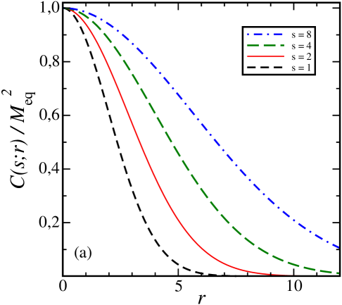
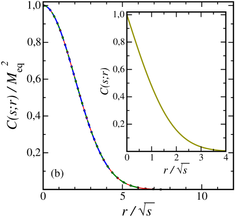
Figure 1: Ageing of the phase-ordering in the single-time correlator $C(s;r)$ in the (mean) spherical model in $d>2$ dimensions. The inset in panel (b) shows the form of the scaling function for a scalar order-parameter and the agreement with Porod’s law.

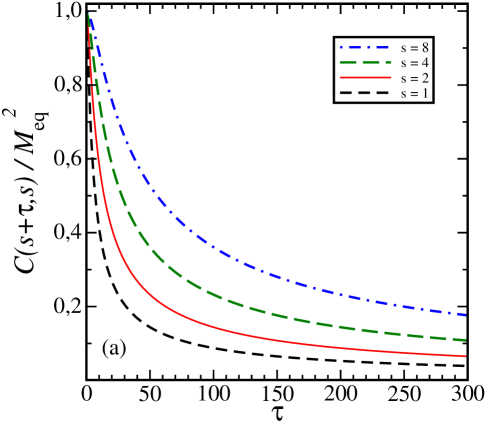
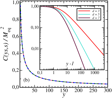
Figure 2: Ageing of the phase-ordering in the two-time auto-correlator $C(t,s)$ in the $3D$ (mean) spherical model, see Henk25V . The inset in panel (b) shows the form of the scaling function for dimensions $d=[3,5,7]$ from top to bottom.

In figures 1 and 2 the further content of eqs. (1) for phase-ordering kinetics is illustrated. Figure 1a shows the single-time auto-correlator $C(s;r)$, normalised by the equilibrium magnetisation $M_{\rm eq}^{2}$, for several times $s$. The first defining property of ageing Stru78 ; Henk10 , namely slow dynamics, appears since for increasing times $s$, the correlator decays more slowly. The second property, absence of time-translation-invariance, is obvious since there is a distinct curve for each value of $s$. The third property, dynamical scaling, is displayed in figure 1b, via the data collapse when the same data are replotted over against $r/\ell(s)$. We see that $\ell(s)\sim s^{1/2}$, in agreement with the expected value $\mathpzc{z}=2$ Bray94b for phase-ordering when the dynamics of the order-parameter $\phi$ does not obey any macroscopic conservation law (one speaks of model-A-type dynamics). The shape of the scaling function in figure 1b reflects the fact that the spherical model spins and their interfaces are quite ‘soft’ such that $C(s;r)$ is rounded-off close to $r\approx 0$, as it occurs for vector-valued order-parameters. For systems with ‘hard’ interfaces, typical for scalar order-parameters, such as in the Glauber-Ising universality class, one rather observes a cusp at $r\approx 0$ as illustrated in the inset of figure 1b. This cusp-like behaviour is known as Porod’s law Poro51 . Experimentally, known examples for scalar model-A-dynamics occur in liquid crystals Alme21 and, with an anti-ferromagnetic order-parameter, in the binary alloy Cu₃Au Shan92 .

Figure 2 presents the same kind of analysis for the two-time autocorrelator $C(ys,s)$. The first two properties of ageing, slow dynamics and absence of time-translation-invariance, are displayed in figure 2a where $C$ is plotted over against the time different $\tau=t-s$, and the third property of the data collapse of dynamical scaling is shown in figure 2b when the same data are replotted over against $y=t/s$. The inset further illustrates the form of this $s$-independent scaling function $f_{C}(y)=C(ys,s)$. The overall form is (i) quite similar for all spatial dimensions $d$ and furthermore, (ii) for $y\gg 1$ one generically finds a power-law $f_{C}(y)\sim y^{-\lambda_{C}/2}$, where $\lambda_{C}$ is the autocorrelation exponent Huse89 . The totality of the observations from figures 1,2 can be condensed into the single scaling form quoted in (1a). The scaling function $F_{C}$ is expected to be universal Bray90 ; Bray94a , which means that its form should be independent of ‘microscopic details’ such as the lattice structure, the precise form of the interactions or the value of $T$. It does depend, however, on the spatial dimension $d$ and on the nature of the order-parameter (e.g. its symmetries).

Similar observations can also be made for the response function and lead to (1b), where $a$ is an ageing exponent. For the auto-reponse scaling function, there is a power-law for $y\gg 1$, viz. $f_{R}(y)=s^{1+a}R(ys,s)\sim y^{-\lambda_{R}/2}$, where $\lambda_{R}$ is the $d$-dependent autoresponse exponent. The scaling function $F_{R}$ is expected universal as well and for spatially short-ranged initial correlations, one finds $\lambda=\lambda_{C}=\lambda_{R}$. In (1b) we also anticipate Janssen-de Dominicis non-equilibrium field theory which allows to rewrite the response functions formally as a correlator with a so-called response scaling operator Jans76 ; Domi76 .

Rather than studying any specific theory of phase-ordering kinetics, we inquire about generic deteriminations of the universal scaling functions $F_{C,R}$. Symmetry arguments are an obvious candidate. They should lead to an understanding of the scaling forms (1) and the properties of the scaling functions $F_{C,R}$. Since the dynamical exponent $\mathpzc{z}=2$, a promising candidate for a larger set of dynamical symmetries might appear to be Schrödinger-transformations, already discovered by Jacobi and by Lie in the 19^th century, and defined as

$$t\mapsto t^{\prime}=\frac{\alpha t+\beta}{\gamma t+\delta}\;\;,\;\;\bm{r}\mapsto\bm{r}^{\prime}=\frac{\mathscr{R}\bm{r}+\bm{v}t+\bm{a}}{\gamma t+\delta}\;\;;\;\;\alpha\delta-\beta\gamma=1$$ (2)

where $\mathscr{R}\in\mbox{\sl SO}(d)$ is a rotation matrix and $\bm{v},\bm{a}\in\mathbb{R}^{d}$ are vectors. For a historical review, see Duva24 . Certainly, time-translations are included therein and further considerations will be needed to render the usual Schrödinger-transformations (2) applicable to non-equilibrium ageing. This will be described in the next section.

2 Background: field-theory & dynamical symmetry

The forthcoming discussion of the scaling form (1), for phase-ordering kinetics, in section 3 will rely on field-theoretic methods and a new adaptation of Schrödinger-invariance Henk25e . We refer to the detailed exposition of these techniques in Henk25V (done there mainly for non-equilibrium critical dynamics after a quench onto $T=T_{c}$) and shall limit ourselves to indicating the necessary differences.

1. Physical ageing must be set into the context of non-equilibrium continuum field-theory Domi76 ; Jans76 ; Taeu14 . In principle, one calculates the average of an observable $\mathscr{A}$ via a functional integral $\bigl\langle\mathscr{A}\bigr\rangle=\int\mathscr{D}\phi\mathscr{D}\widetilde{\phi}\;\mathscr{A}[\phi]\,e^{-{\cal J}[\phi,\widetilde{\phi}]}$. For phase-ordering kinetics, with non-conserved model-A-type dynamics of the order-parameter, one has ${\cal J}[\phi,\widetilde{\phi}\,]={\cal J}_{0}[\phi,\widetilde{\phi}\,]+{\cal J}_{b}[\widetilde{\phi}\,]$ for the Janssen-de Dominicis action where

$${\cal J}_{0}[\phi,\widetilde{\phi}\,] =\int\!{\rm d}t{\rm d}\bm{r}\>\left(\widetilde{\phi}\left(\partial_{t}-\Delta_{\bm{r}}-V^{\prime}[\phi]\right)\phi\right)$$ (3a)

$${\cal J}_{b}[\widetilde{\phi}\,] =-\frac{1}{2}\int_{\mathbb{R}^{2d}}\!{\rm d}\bm{R}{\rm d}\bm{R}^{\prime}\>\widetilde{\phi}(0,\bm{R})C_{0}\bigl(\bm{R}-\bm{R}^{\prime}\bigr)\widetilde{\phi}(0,\bm{R}^{\prime})$$ (3b)

with the interaction $V^{\prime}[\phi]$ and the spatial laplacian $\Delta_{\bm{r}}$ (and the usual re-scalings). Any noise comes only from the spatially short-ranged ‘initial’ correlator $C_{0}\bigl(\bm{R}\bigr)$. The deterministic action ${\cal J}_{0}[\phi,\widetilde{\phi}\,]$ gives rise to the deterministic average $\bigl\langle\mathscr{A}\bigr\rangle_{0}=\int\mathscr{D}\phi\mathscr{D}\widetilde{\phi}\;\mathscr{A}[\phi]\,e^{-{\cal J}_{0}[\phi,\widetilde{\phi}]}$. This is important because either causality Jans76 ; Cala05 ; Taeu14 or the combination of Galilei- and spatial translation-invariance Pico04 of ${\cal J}_{0}[\phi,\widetilde{\phi}\,]$ imply the Bargman superselection rules $\left\langle\overbrace{~\phi\cdots\phi~}^{\mbox{\rm~~$n$ times~~}}\overbrace{~\widetilde{\phi}\cdots\widetilde{\phi}~}^{\mbox{\rm~~$m$ times~~}}\right\rangle_{0}\sim\delta_{n,m}$ Barg54 . Non-vanishing deterministic averages must have an equal number of order-parameters $\phi$ and conjugate response operators $\widetilde{\phi}$. Examples are two-point response functions (see 1b)) $R=\bigl\langle\phi\widetilde{\phi}\bigr\rangle=\bigl\langle\phi\widetilde{\phi}\bigr\rangle_{0}$ or four-point responses $\bigl\langle\phi\phi\widetilde{\phi}\widetilde{\phi}\bigr\rangle=\bigl\langle\phi\phi\widetilde{\phi}\widetilde{\phi}\bigr\rangle_{0}$. On the other hand, a correlator $\left\langle\phi\phi\right\rangle$ must be obtained from a four-point response function

$$\hskip-25.6073ptC(t,s;r)=\bigl\langle\phi(t,\bm{r}+\bm{r}_{0})\phi(s,\bm{r}_{0})\bigr\rangle=\int\mathscr{D}\phi\mathscr{D}\widetilde{\phi}\;\phi(t,\bm{r}+\bm{r}_{0})\phi(s,\bm{r}_{0})\,e^{-{\cal J}_{0}[\phi,\widetilde{\phi}]-{\cal J}_{b}[\widetilde{\phi}]}~~$$ (4)

$$= \bigl\langle\phi(t,\bm{r}+\bm{r}_{0})\phi(s,\bm{r}_{0})e^{-{\cal J}_{b}[\widetilde{\phi}]}\bigr\rangle_{0}$$

$$= \frac{1}{2}\int_{\mathbb{R}^{2d}}\!\!\!{\rm d}\bm{R}{\rm d}\bm{R}^{\prime}\>C_{0}\bigl(\bm{R}-\bm{R}^{\prime}\bigr)\left\langle\phi(t,\bm{r}+\bm{r}_{0})\phi(s,\bm{r}_{0})\widetilde{\phi}(\varepsilon,\bm{R})\widetilde{\phi}(\varepsilon^{\prime},\bm{R}^{\prime})\right\rangle_{0}$$

by expansion to all orders of the exponential $e^{-{\cal J}_{b}[\widetilde{\phi}]}$ of which a single contribution will remain Pico04 ; Henk10 . This replaces (Henk25V, , eq. (4)) in the case of phase-ordering and will serve as our starting point. In (4) $\varepsilon,\varepsilon^{\prime}$ are ‘initial’ time-scales, to be fixed later.

2. The Schrödinger group is known to be the maximal finite-dimensional symmetry of the free Schrödinger equation $\mathscr{S}\phi=\bigl(2{\cal M}\partial_{t}-\Delta_{\bm{r}}\bigr)\phi=0$ in the sense that it maps any solution of that equation onto another solution. This implies that the deterministic action ${\cal J}_{0}[\phi,\widetilde{\phi}]$ is Schrödinger-invariant, as shown explicitly for free fields Henk03a or the $(1+1)D$ Calogero model Shim21 . Since the Lie algebra which follows from (2) is not semi-simple, its representations must be projective and we refer to Henk25V for the explicit generators. For the standard representation of the Schrödinger Lie algebra, the order-parameter $\phi$ is characterised by a scaling dimension $\delta$. Then the hypothesis of Schrödinger-covariance leads to the two-point function ($\mathscr{R}_{0}$ is a normalisation constant) Henk94

$$R(t_{a},t_{b};r)=\left\langle\phi_{a}(t_{a},\bm{r})\widetilde{\phi}_{b}(t_{b},\bm{0})\right\rangle_{0}$$ (5)

$$= \mathscr{R}_{0}\,\delta({\cal M}_{a}+\widetilde{\cal M}_{b})\,\delta_{\delta_{a},\widetilde{\delta}_{b}}\>\Theta(t_{a}-t_{b})\bigl(t_{a}-t_{b}\bigr)^{-2\delta_{a}}\exp\left[-\frac{{\cal M}_{a}}{2}\frac{\bm{r}^{2}}{t_{a}-t_{b}}\right]$$

Response operators $\widetilde{\phi}$ have negative masses $\widetilde{\cal M}_{b}=\widetilde{\cal M}=-{\cal M}=-{\cal M}_{a}<0$. In addition, there is the constraint $\widetilde{\delta}=\delta$ between the scaling dimension of the response operator and the order-parameter. The generic Schrödinger-covartiant four-point function is Golk14 ; Shim21 ; Volo09

$$\left\langle\phi(t,\bm{r})\phi(s,\bm{0})\widetilde{\phi}(0,\bm{R})\widetilde{\phi}(0,\bm{R}^{\prime})\right\rangle_{0}$$ (6)

$$\simeq \bigl(ts\bigr)^{-2\delta}\exp\left[-\frac{\cal M}{2}\frac{\bm{r}^{2}}{t-s}-{\cal M}\frac{\mathfrak{R}^{2}+\overline{\mathfrak{R}}^{2}}{s}\right]\mathscr{F}^{(2)}\left(\frac{\mathfrak{R}}{s^{1/2}}+\frac{1}{y}\frac{\bm{r}}{s^{1/2}},\frac{\overline{\mathfrak{R}}}{s^{1/2}}\right)$$

with the new space variables $\mathfrak{R}=\frac{1}{2}\bigl(\bm{R}+\bm{R}^{\prime}\bigr)$ and $\overline{\mathfrak{R}}=\frac{1}{2}\bigl(\bm{R}-\bm{R}^{\prime}\bigr)$ and $y=t/s$. We shall also need the so-called ‘pairwise equal-time case’ when $t=s>0$ and Shim21

$$\left\langle\phi(s,\bm{r})\phi(s,\bm{0})\widetilde{\phi}(0,\bm{R})\widetilde{\phi}(0,\bm{R}^{\prime})\right\rangle_{0}$$ (7)

$$\simeq s^{-4\delta}\exp\left[-{\cal M}\frac{\mathfrak{R}^{2}+\overline{\mathfrak{R}}^{2}}{s}+{\cal M}\frac{\bm{r}\cdot\mathfrak{R}}{s}\right]\mathscr{F}^{(1)}\left(\frac{\bm{r}\cdot\overline{\mathfrak{R}}}{s}\right)$$

where $\mathscr{F}^{(1,2)}$ are undetermined (differentiable) functions of one/two arguments, respectively, which are not fixed by Schrödinger-covariance alone. These expressions were directly written in the scaling limit

$$s\to\infty\;\;,\;\;\tau=t-s=(y-1)s\to\infty\;\;,\;\;\bm{r},\bm{R},\bm{R}^{\prime}\to\infty$$ (8a)

such that the following quantities are kept finite

$$y=\frac{t}{s}>1\;\;,\;\;\frac{\bm{r}}{s^{1/2}}\;\;,\;\;\frac{\bm{R}}{s^{1/2}}\;\;,\;\;\frac{\bm{R}^{\prime}}{s^{1/2}}$$ (8b)

In both (6,7), the time-scale ‘$0$’ of the response operators $\widetilde{\phi}$ is meant as a short-hand for an ‘initial’ time-scale $\varepsilon\ll s,t$, to be specified below. Finally, for applications which involve finite-size effects, one may reuse (6) but with the finite-size scaling function $\mathscr{F}^{(2,N)}\left(\frac{\mathfrak{R}}{s^{1/2}}+\frac{1}{y}\frac{\bm{r}}{s^{1/2}},\frac{\overline{\mathfrak{R}}}{s^{1/2}},\frac{t^{1/2}}{N}\right)$ for $t\gg s$ Henk25e .

3. The expressions (6,7) for the two- and four-point response are brought out-of-equilibrium by the following

Postulate: Henk25 ; Henk25c The Lie algebra generator $X_{n}^{\rm equi}$ of a time-space symmetry of an equilibrium system becomes a symmetry out-of-equilibrium by the change of representation

$$X_{n}^{\rm equi}\mapsto X_{n}=e^{\xi\ln t}X_{n}^{\rm equi}e^{-\xi\ln t}$$ (9)

where $\xi$ is a dimensionless parameter whose value contributes to characterise the scaling operator $\phi$ on which $X_{n}$ acts.

For critical dynamics, at $T=T_{c}$, this is suggestive since one may consider this as a generalisation of known equilibrium dynamical symmetries Card85 . In that case, there a numerous practical examples, reviewed in Henk25V , which suggest that the method might work successfully. For phase-ordering at $T<T_{c}$, however, despite the well-established non-equilibrium dynamical scaling Bray90 ; Bray94a , it is less obvious that our postulate should work and does require separate testing Henk25e .

Formally, when applied to the dilatation generator $X_{0}^{\rm equi}=-t\partial_{t}-\delta$ this leads to

$$X_{0}^{\rm equi}\mapsto X_{0}=-t\partial_{t}-\frac{1}{\mathpzc{z}}r\partial_{r}-\bigl(\delta-\xi\bigr)$$ (10a)

which means that one has an effective scaling dimension $$\delta_{\rm eff}=\delta-\xi X_{-1}^{\rm equi}=-\partial_{t}$$. The time-translation generator turns into

$$X_{-1}^{\rm equi}\mapsto X_{-1}=-\partial_{t}+\frac{\xi}{t}$$ (10b)

which makes the result of an application of $X_{-1}$ appear non-trivial. Significantly, in this new representation the scaling operators become $\Phi(t)=t^{\xi}\phi(t)=e^{\xi\ln t}\phi(t)$ which will be identified as the ‘physical’ ones. The above equilibrium response functions, found from covariance under the standard representation of the Schrödinger Lie algebra Henk25V , now read (spatial arguments are suppressed for clarity)

$$\bigl\langle\phi_{a}(t_{a})\widetilde{\phi}_{b}(t_{b})\bigr\rangle_{0} \mapsto t_{a}^{\xi_{a}}t_{b}^{\widetilde{\xi}_{b}}\>\bigl\langle\phi_{a}(t_{a})\widetilde{\phi}_{b}(t_{b})\bigr\rangle_{0}$$

$$\bigl\langle\phi_{a}(t_{a})\phi_{b}(t_{b})\widetilde{\phi}_{c}(t_{c})\widetilde{\phi}_{d}(t_{d})\bigr\rangle_{0} \mapsto t_{a}^{\xi_{a}}t_{b}^{\xi_{b}}t_{c}^{\widetilde{\xi}_{c}}t_{d}^{\widetilde{\xi}_{d}}\>\bigl\langle\phi_{a}(t_{a})\phi_{b}(t_{b})\widetilde{\phi}_{c}(t_{c})\widetilde{\phi}_{d}(t_{d})\bigr\rangle_{0}$$ (11)

Now, we characterise a non-equilibrium scaling operator $\phi$ by a pair of scaling dimensions $(\delta,\xi)$ and a non-equilibrium response operator $\widetilde{\phi}$ by a pair $(\widetilde{\delta},\widetilde{\xi})$. The Bargman rule with $n=m=1$ implies $\delta=\widetilde{\delta}$ but $\xi$ and $\widetilde{\xi}$ remain independent.

Finally, for the two-time autocorrelator $C(t,s)=\langle\phi_{1}\phi_{2}\rangle=\langle\phi(t)\phi(s)\rangle$ the scaling operator identity $\phi_{1}=\phi_{2}=\phi$ implies for the scaling dimensions $\delta_{1}=\delta_{2}=\delta$ and $\xi_{1}=\xi_{2}=\xi$. This produces the exponent relations Henk25c

$$\frac{\lambda}{2}=2\delta-\xi\;\;,\;\;\delta=\xi$$ (12)

4. Once correlated domains have formed, the effective equation of motion is no longer the one derived from the action (3) which becomes unstable rapidly Bray94a but will rather take an effective form $\mathscr{S}^{\rm equi}\phi=\left(\partial_{t}-\frac{1}{2{\cal M}}\Delta_{\bm{r}}\right)\phi(t,\bm{r})=g\phi^{3}(t,\bm{r})$. The plausibility of this form is argued as follows Henk25c :

1. a term linear in $\phi(t,\bm{r})$ on its right-hand-side would break dynamical scaling

2. a term quadratic in $\phi(t,\bm{r})$ breaks the global spin-reversal-invariance $\phi\mapsto-\phi$

3. a term cubic in $\phi(t,\bm{r})$ is the lowest-order term which may appear

4. thermal noise will merely lead to corrections to scaling

5. the exponent $\mathpzc{z}=2$ Bray94b for short-ranged model-A-type dynamics

Our postulate implies the modified form of the Schrödinger operator $\mathscr{S}^{\rm equi}=\partial_{t}-\frac{1}{2{\cal M}}\Delta_{\bm{r}}$

$${\mathscr{S}}=e^{\xi\ln t}\mathscr{S}^{\rm equi}e^{-\xi\ln t}=\partial_{t}-\frac{\xi}{t}-\frac{1}{2{\cal M}}\Delta_{\bm{r}}$$ (13)

and contains an additional $1/t$-potential which is well-known from the literature Oono88 ; Maze06 . Because of $\left(t^{\xi}\,\mathscr{S}^{\rm equi}\,t^{-\xi}\right)\left(t^{\xi}\,\phi\right)=g\,t^{\xi}\left(t^{-\xi}\,{\Phi}\,\right)^{3}$ we find

$${\mathscr{S}}\,{\Phi}=\left(\partial_{t}-\frac{\xi}{t}-\frac{1}{2{\cal M}}\Delta_{\bm{r}}\right){\Phi}=g\,t^{-2\xi}\,{\Phi}^{\,3}$$ (14)

For phase-ordering kinetics, (12) implies that $\delta_{\rm eff}=\delta-\xi=0$ such that ${\Phi}$ is dimensionless, such that the long-time behaviour of (14) is governed by the explicit $t$-dependence. The $1/t$-potential will for large times dominate over against the non-linear term, when the criterion Henk25c ; Henk25e

$$2\xi>1~~\Longleftrightarrow~~\lambda>1$$ (15)

is satisfied. For its validity in models, recall the well-known auto-correlation bound $\lambda\geq d/2$ Fish88a ; Yeun96a . Hence for $d>2$, the criterion (15) is satisfied. For $d=2$, one has typically $\lambda\approx 1.25>1$ (see Henk10 and refs. therein) and (15) is satisfied as well. Although the effective equation of motion of phase-ordering need not be Schrödinger-invariant, we may use the Schrödinger symmetry of the linear part of (14), with the additional $1/t$-potential, to deduce its long-time behaviour. Of course, this linearised equation cannot be used for a first-principles calculation of exponents such as $\lambda,a,\ldots$ for which the full equation of motion must be used Maze06 .

3 Results

We shall concentrate on the analysis of the correlators by using (4) as the starting point. Concerning the two-time response function, we merely mention the well-known fact that Schrödinger-covariance does reproduce $f_{R}(y)\sim y^{-\lambda_{R}/2}$ for $y\gg 1$ and that $\lambda:=\lambda_{R}=\lambda_{C}$ Henk06 ; Henk25c . In addition, in phase-ordering kinetics, in all known models one has $\delta=\xi=-\widetilde{\xi}$.

1. We begin with the two-time auto-correlator $C(ys,s)$. Combining (4,6,11) and setting $\bm{r}=\bm{0}$, we find

$$C(ys,s;\bm{0})=\!\int_{\mathbb{R}^{2d}}\!\!{\rm d}\mathfrak{R}{\rm d}\overline{\mathfrak{R}}\>C_{0}\bigl(2\overline{\mathfrak{R}}\bigr)\,y^{-2\delta+\xi}s^{2\xi-4\delta}\varepsilon^{2\widetilde{\xi}}\>e^{-\frac{{\cal M}}{s}\bigl(\mathfrak{R}^{2}+\overline{\mathfrak{R}}^{2}\bigr)}$$

$$\hskip 28.45274pt\times~~\mathscr{F}^{(2)}\left(\mathfrak{R}\frac{(s-1)^{1/2}}{s},\overline{\mathfrak{R}}\frac{(s-1)^{1/2}}{s}\right)$$

$$\simeq y^{-2\delta+\xi}\,s^{2(\xi-\delta)}\,s^{-2\delta+d}\varepsilon^{2\widetilde{\xi}}\underbrace{\int_{\mathbb{R}^{2d}}\!{\rm d}\bm{U}{\rm d}\overline{\bm{U}}\>C_{0}\bigl(2\overline{\bm{U}}s^{1/2}\bigr)e^{-{\cal M}\bigl(\bm{U}^{2}+\overline{\bm{U}}^{2}\bigr)}\,\mathscr{F}^{(2)}\bigl(\bm{U},\overline{\bm{U}}\bigr)}_{\to~\mathscr{C}^{(2)}_{\infty}}$$

where in the second line, we first let $s\gg 1$ and then changed the integration variables. In what follows, we shall always assume that the initial correlator $C_{0}\bigl(\bm{R}\bigr)$ as well as the scaling function $\mathscr{F}^{(2)}\bigl(\bm{U},\overline{\bm{U}}\bigr)$ are such that in the indicated limit of large waiting times $s\gg 1$ the integral tends towards a finite, non-vanishing constant $\mathscr{C}^{(2)}_{\infty}$. Furthermore, as inspired by the studies in Zipp00 ; Andr06 , we admit that the ‘initial’ time-scale at the beginning of the scaling regime is related to the waiting time $s$ as

$$\varepsilon\simeq\varepsilon_{0}\,s^{\zeta_{p}}$$ (17)

where $\zeta_{p}$ is a new exponent supposed to describe the beginning of the scaling regime. With these assumptions, the leading large-time behaviour (3) of the two-time auto-correlator becomes

$$C(ys,s)=y^{-(2\delta-\xi)}\,s^{2(\xi-\delta)}\,s^{d-2\delta+2\zeta_{p}\widetilde{\xi}}\>\varepsilon_{0}\,\mathscr{C}^{(2)}_{\infty}$$ (18)

This already reproduces (i) the algebraic behaviour (1a) of the two-time correlator for $y=t/s\gg 1$, and (ii) also shows that $\frac{\lambda_{C}}{2}=2\delta-\xi=\frac{\lambda_{R}}{2}$, as expected. Since for phase-ordering kinetics, one has (12) and $\delta=\xi=-\widetilde{\xi}$. The scaling (18) becomes $s$-independent, as expected from (1a), if we have the new scaling relation Henk25e

$$2\delta=\frac{d}{1+\zeta_{p}}=\lambda$$ (19)

This scaling relation is distinct with respect to non-equilibrium critical dynamics. It underscores the non-trivial nature of the auto-correlation exponent $\lambda$.

For the passage exponent, one has obviously $\zeta_{p}\geq 0$ and also $\zeta_{p}\leq 1$ since the ageing regime cannot start later than at the waiting time $s$ itself. This reproduces the well-known bounds $\frac{d}{2}\leq\lambda\leq d$, from the literature Fish88a ; Yeun96a .

2. Now, we set $t=s$, combine (4,7,11) and have the single-time correlator

$$C(s;r)=\int_{\mathbb{R}^{2d}}\!{\rm d}\mathfrak{R}{\rm d}\overline{\mathfrak{R}}\>C_{0}\bigl(2\overline{\mathfrak{R}}\bigr)\>e^{-\frac{{\cal M}}{s}\bigl(\mathfrak{R}^{2}+\overline{\mathfrak{R}}^{2}\bigr)+\frac{\cal M}{s}r\,\mathfrak{R}}\,s^{2\xi-4\delta}\varepsilon^{2\widetilde{\xi}}\mathscr{F}^{(1)}\left(\frac{\bm{r}\cdot\overline{\mathfrak{R}}}{s}\right)$$ (20)

$$= e^{-\frac{\cal M}{4}\frac{r^{2}}{s}}\,s^{2\xi-4\delta+\frac{d}{2}-2\xi\zeta_{p}}\int_{\mathbb{R}^{d}}\!{\rm d}\overline{\mathfrak{R}}\>C_{0}\bigl(2\overline{\mathfrak{R}}\bigr)\>e^{-\frac{\cal M}{s}\overline{\mathfrak{R}}^{2}}\,\mathscr{F}^{(1)}\left(\frac{\bm{r}}{s^{1/2}}\cdot\frac{\overline{\mathfrak{R}}}{s^{1/2}}\right)$$

$$= e^{-\frac{\cal M}{4}\frac{r^{2}}{s}}\>\int_{\mathbb{R}^{d}}\!{\rm d}\overline{\bm{U}}\>C_{0}\bigl(2\overline{\bm{U}}\,s^{1/2}\bigr)\>e^{-{\cal M}\overline{\bm{U}}^{2}}\,\mathscr{F}^{(1)}\left(\frac{\bm{r}}{s^{1/2}}\cdot\overline{\bm{U}}\right)$$

Herein, we introduced the ‘initial’ time estimate (17), completed a square in the $\mathfrak{R}$-integration, and applied again he scaling relation (19). If the same kind of limit as before exists and is finite, we have again reproduce the scaling form (1), now for $t=s$ and identify the scaling function $F_{C}$ with the natural scaling variable $r/\sqrt{s\,}$.

An explicit computation of the function $F_{C}(1,r/\sqrt{s\,}\,)$ must await stronger information on $\mathscr{F}^{(1)}$ than is currently available. If a limited analytic expansion of $\mathscr{F}^{(1)}$ for small arguments is possible, we would find an expansion of $C(s;r)$ for small $r$

$$C\bigl(s;|\bm{r}|\bigr)\simeq\exp\left[{-\frac{\cal M}{4}\frac{r^{2}}{s}}\right]\int_{\mathbb{R}^{d}}\!{\rm d}\overline{\bm{U}}\>C_{0}\bigl(2\overline{\bm{U}}s^{1/2}\bigr)\>e^{-{\cal M}\overline{\bm{U}}^{2}}\,\left(\mathscr{F}_{0}^{(1)}+\mathscr{F}_{1}^{(1)}\,\overline{\bm{U}}\cdot\frac{\bm{r}}{s^{1/2}}+\ldots\right)$$ (21)

If the corresponding integrals have finite limits for $s\gg 1$ and if $\mathscr{F}_{1}^{(1)}<0$, this would reproduce the typical small-distance behaviour $C(s;|\bm{r}|)\simeq C_{0}-C_{1}\frac{|\bm{r}|}{s^{1/2}}+\ldots$ for a scalar order-parameter, with a cusp at $r=0$. This is illustrated in the inset of figure 1b and the observed linear behaviour is predicted by Porod’s law Poro51 ; Bray94a . A recent simulation illustrates this in Chris19 , and for a classic example see (Bray94a, , fig. 14).

Remarkably, single-time and two-time correlators are treated on the same conceptual basis, namely the covariance of the four-point response function $\langle\phi\phi\widetilde{\phi}\widetilde{\phi}\rangle$.

3. We use (20) in the definition of the structure factor and find

$$\widehat{S}(s;\bm{q}) := \int_{\mathbb{R}^{d}}\!{\rm d}\bm{r}\>e^{-{\rm i}\bm{q}\cdot\bm{r}}\>C(s;\bm{r})=s^{d/2}\mathpzc{g}\left(\bm{q}s^{1/2}\right)\>=\>\ell(s)^{d}\bar{\mathpzc{g}}\bigl(\bm{q}\ell(s)\bigr)$$ (22)

the required scaling form Bray94a , with scaling functions $\mathpzc{g}$ or $\bar{\mathpzc{g}}$, and the length scale $\ell=\ell(s)\sim s^{1/2}$. This is based on the same assumptions on $C_{0}\bigl(\bm{R}\bigr)$ and $\mathscr{F}^{(1)}$ as before.

In the limit $|\bm{q}|\to\infty$, this should be compatible with Porod’s law Poro51 ; Bray94a . It is one of the central ingredients in the derivation of $\mathpzc{z}=2$ for model-A-type dynamics in phase ordering Bray94b . Indeed, on the basis of the expansion carried out in (21), it can be shown that for large momenta $\bm{Q}=\bm{q}s^{1/2}\to\infty$, one obtains $\mathpzc{g}(\bm{Q})\sim|\bm{Q}|^{-d-1}$ which is indeed the form in which Porod’s law is usually stated.

[width=0.3]actes_varnaLT16-taillefinie.eps

Figure 3: Autocorrelator $C(ys,s)$ in a fully finite system.

4. We now consider a fully finite system, say in a hypercubic geometry with a side of linear length $N$. A typical autocorrelator $C(ys,s)$ is shown in figure 3. For large system sizes $N\to\infty$, one recovers the behaviour of the infinite-size system, with its power-law decay $f_{C}(y)\sim y^{-\lambda/2}$ (dashed line). For $N$ small, the correlator decreases with $y$ faster than in the infinite-size limit, before for $y=t/s\gg 1$ it crosses over to a plateau (full line). Its height $C_{\infty}^{(2)}$ should scale with $s$ and with $N$.

The corresponding scaling laws are found by repeating the same steps in the calculation of the correlator which led above to (3). Now, we use instead the finite-size scaling function $\mathscr{F}^{(2,N)}$, together with the scaling relation (19). For $t=ys\gg s>0$, the two-time auto-correlator can be written in the form Henk25e

$$C\left(ys,s;\bm{0};\frac{1}{N}\right) = y^{-\delta}\int_{\mathbb{R}^{2d}}\!{\rm d}\bm{U}{\rm d}\overline{\bm{U}}\>C_{0}\bigl(2\overline{\bm{U}}s^{1/2}\bigr)\>e^{-{\cal M}\bigl(\bm{U}^{2}+\overline{\bm{U}}^{2}\bigr)}\mathscr{F}^{(2,N)}\left(\bm{U},\overline{\bm{U}},\frac{\bigl(ys\bigr)^{1/2}}{N}\right)$$ (23)

$$\simeq y^{-\delta}\mathscr{F}_{C}\left(\frac{N}{\bigl(ys\bigr)^{1/2}}\right)$$

where the finite-size scaling form in the second line holds in the scaling limit (8). We recover the known result $\delta=\lambda/2$.

The limit behaviour illustrated in figure 3 fixes the finite-size scaling behaviour of $\mathscr{F}_{C}$, or equivalently the dependence on the third scaling variable of the scaling function $\mathscr{F}^{(2,N)}$. Clearly, for $N\gg t^{1/2}=\bigl(ys\bigr)^{1/2}$, the system will behave as being spatially infinite. In that limit, $\mathscr{F}_{C}$ should become a constant and the scaling function $\mathscr{F}^{(2,N)}\bigl(.,.,\mathfrak{u}\bigr)$ is expected to become independent of $\mathfrak{u}$. On the other hand, for finite systems one expects $N\lesssim t^{1/2}$ such that the $y$-independent plateau is reached. This implies $\mathscr{F}_{C}(\mathfrak{u})\sim\mathfrak{u}^{-\lambda}$ or equivalently $\mathscr{F}^{(2,N)}\bigl(.,.,\mathfrak{u}\bigr)\sim\mathfrak{u}^{\lambda}$. Summarising, the plateau height $C_{\infty}^{(2)}=\lim_{s\to\infty}C\bigl(ys,s;\bm{0};\frac{1}{N}\bigr)$ should scale as

$$C_{\infty}^{(2)}\sim\left(\frac{t}{s}\right)^{-\lambda/2}\left(\frac{t^{1/2}}{N}\right)^{\lambda}\sim N^{-\lambda}s^{\lambda/2}$$ (24)

and in particular, we should have the finite-size scaling behaviour

$$C_{\infty}^{(2)}\sim\left\{\begin{array}[]{ll}N^{-\lambda}&\mbox{\rm if $s$ is kept fixed}\\ s^{\lambda/2}&\mbox{\rm if $N$ is kept fixed}\end{array}\right.$$ (25)

which reproduce Henk25c for the special case of quenches to $0<T<T_{c}$ and for $\mathpzc{z}=2$.

Available tests of this in specific models have been discussed in detail in Henk25c . There are no known well-studied finite-size effects in the single-time correlator.

5. The global two-time correlator for $t>s$ is obtained by integrating the two-time correlator $C(t,s;\bm{r})$ with respect to $\bm{r}$. Combining (4,6,11) leads to Henk25e

$$\widehat{C}(t,s;\bm{0})=\int_{\mathbb{R}^{d}}\!{\rm d}\bm{r}\>C(t,s;\bm{r})$$

$$\simeq s^{d/2}\left(\frac{t}{s}\right)^{\Theta}\underbrace{~\int_{\mathbb{R}^{3d}}\!{\rm d}\bm{u}{\rm d}\bm{U}{\rm d}\overline{\bm{U}}\>C_{0}\bigl(2\overline{\bm{U}}s^{1/2}\bigr)\>e^{-\frac{\cal M}{2}\bm{u}^{2}-{\cal M}\bigl(\bm{U}^{2}+\overline{U}^{2}\bigr)}\,\mathscr{F}^{(2)}\left(\bm{U}+\bm{u}y^{-1/2},\overline{\bm{U}}\right)~}_{=~\mbox{\rm\footnotesize cste.}}~~~~~$$

where in the last line we let $t\gg s$, used as before that $\delta=\xi=-\widetilde{\xi}$ and also the scaling relation (19) about $\zeta_{p}$. As several times before, we also assume that the last integral in (25) converges to a finite non-zero constant in the $s\gg 1$ limit. In particular, the global correlator (3) with the initial state scales as $\widehat{C}(t,0)\sim t^{\Theta}$. Herein, the slip exponent

$$\Theta=\frac{1}{2}\bigl(d-\lambda\bigr)$$ (27)

is given by the extension to $0<T<T_{c}$ of the Janssen-Schaub-Schmittmann (jss) critical-point scaling relation Jans89 , for $\mathpzc{z}=2$, as expected. Certainly, the values of $\Theta,\lambda,\mathpzc{z}$ are in general different for $0<T<T_{c}$ and $T=T_{c}$.

For quenches onto the critical point $T=T_{c}$, the original jss-relation has been the conceptual basis of a whole field of studies on non-equilibrium critical dynamics, called ‘short-time dynamics’, since it is not necessary to carry out simulation to extremely long times, see Alba11 ; Zhen98 for classical reviews. Eq. (27) could serve the same purpose in phase-ordering kinetics after a quench into $T<T_{c}$. An example is Moue25 .

6. For equal times $t=s$, we might use the combination of (4,7,11) and find for the squared magnetisation

$$\hskip-11.38092pt\left\langle m^{2}(s)\right\rangle=\widehat{C}(s,s;\bm{0})=\int_{\mathbb{R}^{d}}e^{-\frac{\cal M}{4}\frac{\bm{r}^{2}}{s}}\int_{\mathbb{R}^{d}}\!{\rm d}\overline{\bm{U}}\>C_{0}\bigl(2\overline{\bm{U}}s^{1/2}\bigr)\>e^{-{\cal M}\overline{\bm{U}}^{2}}\>\mathscr{F}^{(1)}\left(\frac{\bm{r}}{s^{1/2}}\cdot\overline{\bm{U}}\right)$$ (28)

$$= s^{d/2}\underbrace{~\int_{\mathbb{R}^{2d}}\!{\rm d}\bm{u}{\rm d}\overline{\bm{U}}\>C_{0}\bigl(2\overline{\bm{U}}s^{1/2}\bigr)\>\exp\left[-\frac{\cal M}{4}\bm{u}^{2}-{\cal M}\overline{\bm{U}}^{2}\right]\mathscr{F}^{(1)}\left(\bm{u}\cdot\overline{\bm{U}}\right)~}_{=~\mbox{\rm\footnotesize cste.}}$$

and with the usual assumption that the last integral converges to a finite, non-zero constant, we recover the scaling $\langle m^{2}(s)\rangle\sim s^{d/2}$ Jank23 , well-tested in simulations. Of course, one may obtain this scaling also from (3) by taking the $t\to s$ limit.

7. To finish, we discuss the finite-size scaling of the global auto-correlator in a fully finite system of linear size $N$. As above, we expect that the global correlator should converge towards a plateau of height $\widehat{C}_{\infty}^{(2)}$ when $\ell(t)\approx N$ but $\ell(s)\ll N$. Generalising (3) we have, for $t\gg s$ Henk25e

$$\widehat{C}\left(t,s;\bm{0};\frac{1}{N}\right)=\int_{\mathbb{R}^{d}}\!{\rm d}\bm{r}\>C\left(t,s;\bm{r};\frac{1}{N}\right)$$ (29)

$$= s^{d/2}\left(\frac{t}{s}\right)^{\Theta}\int_{\mathbb{R}^{3d}}\!{\rm d}\bm{u}{\rm d}\bm{U}{\rm d}\overline{\bm{U}}\>C_{0}\bigl(2\overline{\bm{U}}s^{1/2}\bigr)\>e^{-\frac{\cal M}{2}\bm{u}^{2}-{\cal M}\bigl(\bm{U}^{2}+\overline{U}^{2}\bigr)}\,\mathscr{F}^{(2,N)}\left(\bm{U}+\bm{u}\frac{s}{t},\overline{\bm{U}},\frac{t^{1/2}}{N}\right)$$

$$\sim s^{d/2-\Theta}N^{2\Theta}$$

and use of course the scaling relation (27). The phenomenological discussion of the limits $N\gg t^{1/2}$ and $N\lesssim t^{1/2}$ in the scaling function $\mathscr{F}^{(2,N)}$ and the scaling of the plateau $\widehat{C}_{\infty}^{(2)}$ is as before and leads to the scaling in the last line of (29). The plateau height scales as follows, predicted before for $0<T<T_{c}$ and $\mathpzc{z}=2$ Henk25c

$$\widehat{C}_{\infty}^{(2)}\sim\left\{\begin{array}[]{ll}N^{2\Theta}&\mbox{\rm if $s$ is kept fixed}\\ s^{d/2-\Theta}&\mbox{\rm if $N$ is kept fixed}\end{array}\right.$$ (30)

4 Conclusions

The complete known phenomenology of phase-ordering kinetics, after a quench into the phase coexistence region, can be derived from the covariance of the multi-point response functions under new non-equilibrium representations of the Schrödinger Lie algebra Henk25e . This reproduces those properties which are well-established folklore and also permits to obtain a couple of new scaling laws. We illustrated this here through a discussion of the two-time and single-time correlation functions.

Acknowledgements: We thank the PHC Rila for financial support (51305UC/KP06-Rila/7). mh was supported by ANR-PRME UNIOPEN (ANR-22-CE30-0004-01).

References

- (1) E.V. Albano, M.A.N. Bab, G. Baglietto, R.A. Borzi, T.S. Grigera, E.S. Loscar, D.E. Rodriguez, M.L. Rubio Puzzo, G.P. Saracco, Rep. Prog. Phys. 74, 026501 (2011).
- (2) R. Almeida, K. Takeuchi, Phys. Rev. E104, 054103 (2021) [arxiv:2107.09043].
- (3) A. Andreanov, A. Lefèvre, Europhys. Lett. 76, 919 (2006) [arXiv:cond-mat/0606574].
- (4) V. Bargman, Ann. of Math. 59, 1 (1954).
- (5) A.J. Bray, Phys. Rev. B41, 6724 (1990).
- (6) A.J. Bray, Adv. Phys. 43 357 (1994), [arXiv:cond-mat/9501089].
- (7) A.J. Bray, A.D. Rutenberg, Phys. Rev. E49, R27 (1994) and E51, 5499 (1995) [arxiv:cond-mat/9303011], [arxiv:cond-mat/9409088].
- (8) P. Calabrese, A. Gambassi, J. Phys. A38, R133 (2005) [arXiv:cond-mat/0410357].
- (9) J.L. Cardy, J. Phys. A18, 2771 (1985).
- (10) H. Christiansen, S. Majumder, W. Janke, Phys. Rev. E99, 011301 (2019) [arXiv:1808.10426].
- (11) L.F. Cugliandolo, in J.-L. Barrat et al. (eds), Slow relaxations and non-equilibrium dynamics in condensed matter, Les Houches 77, Springer (Heidelberg 2003), pp. 367-521 [arxiv:cond-mat/0210312].
- (12) L.F. Cugliandolo, Comptes Rendus Physique 16, 257 (2015) [arXiv:1412.0855].
- (13) C. de Dominicis, J. Physique (Colloque) 37, C1-247 (1976).
- (14) C. Duval, M. Henkel, P. Horvathy, S. Rouhani, P. Zhang, Int. J. Theor. Phys. 63, 184 (2024) [arxiv:2403.20316].
- (15) D.S. Fisher, D.A. Huse, Phys. Rev. B38, 373 (1988).
- (16) C. Godrèche, J.-M. Luck, J. Phys. Cond. Matt. 14, 1589 (2002) [arXiv:cond-mat/0109212].
- (17) S. Golkar, D.T. Son, JHEP 12 (2014) 063 [arxiv:1408.3629].
- (18) M. Henkel, J. Stat. Phys. 75, 1023 (1994), [arxiv:hep-th/9310081].
- (19) M. Henkel, J. Unterberger, Nucl. Phys. B660, 407 (2003) [hep-th/0302187].
- (20) M. Henkel, T. Enss, M. Pleimling, J. Phys. A39, L589 (2006), [arxiv:cond-mat/0605211].
- (21) M. Henkel, M. Pleimling, Non-equilibrium phase transitions vol. 2, Springer (Heidelberg 2010).
- (22) M. Henkel, in V. Dobrev (éd.), Springer Proc. Math. Stat. 473, 93 (2025) [hal-04377461].
- (23) M. Henkel, Nucl. Phys. B1017, 116968 (2025) [arxiv:2504.16857].
- (24) M. Henkel, S. Stoimenov, Nucl. Phys. B1020, 117151 (2025) [arXiv:2508.08963].
- (25) M. Henkel, S. Stoimenov, Schrödinger-invariance in non-equilibrium critical dynamics, these proceedings. Also on [arxiv:2510.25429].
- (26) D.A. Huse, Phys. Rev. B40, 304 (1989).
- (27) W. Janke, H. Christiansen, S. Majumder, Eur. Phys. J. ST 232, 1693 (2023).
- (28) H.K. Janssen, Z. Phys. B23, 377 (1976).
- (29) H.K. Janssen, B. Schaub, B. Schmittmann, Z. Phys. B73, 539 (1989).
- (30) G.F. Mazenko, Nonequilibrium statistical mechanics, Wiley-VCH (Weinheim 2006).
- (31) L. Moueddene, M. Henkel, [arxiv:2511.00498].
- (32) Y. Oono, S. Puri, Mod. Phys. Lett. B2, 861 (1988).
- (33) A. Picone, M. Henkel, Nucl. Phys. B688, 217 (2004); [arxiv:cond-mat/0402196].
- (34) G. Porod, Kolloid-Zeitschrift 124, 83 (1951).
- (35) S. Puri, V. Wadhawan (éds), Kinetics of phase transitions, Taylor and Francis (London 2009).
- (36) R.F. Shannon, Jr., S.E. Nagler, C.R. Harkless, R.M. Nicklow, Phys. Rev. B46, 40 (1992).
- (37) H. Shimada, H. Shimada, JHEP 10(2021)030 [arXiv:2107.07770].
- (38) S. Stoimenov, M. Henkel, Nucl. Phys. B723, 205 (2005) [arxiv:math-ph/0504028].
- (39) L.C.E. Struik, Physical ageing in amorphous polymers and other materials, Elsevier (Amsterdam 1978).
- (40) U.C. Täuber, Critical dynamics, Cambridge University Press (Cambridge 2014).
- (41) A. Volovich, C. Wen, JHEP 05(2009) 087 [arXiv:0903.2455]
- (42) C. Yeung, M. Rao, R.C. Desai, Phys. Rev. E53, 3073 (1996) [arxiv:cond-mat/9409108].
- (43) B. Zheng, Int. J. Mod. Phys. B12, 1419 (1998).
- (44) W. Zippold, R. Kühn, H. Horner, Eur. Phys. J. B13, 531 (2000) [arXiv:cond-mat/9904329].