Search for Diffuse Supernova Neutrino Background
with 956.2 days of Super-Kamiokande Gadolinium Dataset

Abstract

We report the search result for the Diffuse Supernova Neutrino Background (DSNB) in neutrino energies beyond 9.3 MeV in the gadolinium-loaded Super-Kamiokande (SK) detector with $22,500\times 956.2$$~\rm m^{3}\cdot day$ exposure. Starting in the summer of 2020, SK introduced 0.01% gadolinium (Gd) by mass into its ultra-pure water to enhance the neutron capture signal, termed the SK-VI phase. This was followed by a 0.03% Gd-loading in 2022, a phase referred to as SK-VII. We then conducted a DSNB search using 552.2 days of SK-VI data and 404.0 days of SK-VII data through September 2023. This analysis includes several new features, such as two new machine-learning neutron detection algorithms with Gd, an improved atmospheric background reduction technique, and two parallel statistical approaches. No significant excess over background predictions was found in a DSNB spectrum-independent analysis, and 90% C.L. upper limits on the astrophysical electron anti-neutrino flux were set. Additionally, a spectral fitting result exhibited a $\sim 1.2\sigma$ disagreement with a null DSNB hypothesis, comparable to a previous result from 5823 days of all SK pure water phases.

1 Diffuse supernova neutrino background

Core-collapse supernovae (CCSNe) are known as some of the most dynamic phenomena in the Universe. To understand the CCSN mechanism, knowledge of the deep core of the exploding star is essential. Neutrinos are one of the few ways to access the core of a star. Since they are not sensitive to electromagnetic interactions, the information encoded within a neutrino flux is largely unaltered. Owing to this, observing a time-dependent neutrino flux from a CCSN burst could provide important information about the CCSN explosion mechanism (Totani et al., 1998; Kachelrieß et al., 2005; Janka, 2012; Scholberg, 2012; Takiwaki et al., 2014; Mirizzi et al., 2016; Horiuchi & Kneller, 2018; Vartanyan & Burrows, 2023). Despite the growing focus on detecting neutrinos from CCSNe, neutrino detectors are primarily sensitive to those occurring within our own galaxy, which are rare events (Tammann et al., 1994).

Another avenue for studying CCSNe is through the observation of the cumulative neutrino fluxes from all past supernovae in the Universe. This is termed the Diffuse Supernova Neutrino Background (DSNB), or Supernova Relic Neutrinos (SRNs). For most detectors, the target signal channel is the inverse beta decay (IBD) of protons induced by electron antineutrinos due to the large cross-section within the MeV signal range.

The DSNB flux is affected by the cosmological expansion of the Universe, such that it is redshifted before reaching the Earth, and the amount of redshift depends on when each supernova occurred in the history of the Universe. The magnitude of the flux depends heavily on the supernova rate, which can be predicted using astrophysical measurements of the star formation rate (SFR). Therefore, the magnitude and shape of the DSNB flux provide unique information about the cosmic history of massive star formation. The shape of the DSNB flux also results from the combined effect of various factors, such as the equation of state of neutron stars, the shockwave revival time of CCSNe, neutrino propagation in dense matter, and the stellar initial mass function (Beacom, 2010; Lunardini, 2016; Suliga et al., 2022; Ando et al., 2023). In addition, the neutrino mass ordering affects the DSNB spectral shape for each neutrino flavor. Furthermore, potential exotic physics, such as neutrino decay (Tabrizi & Horiuchi, 2021; Iváñez-Ballesteros & Volpe, 2023), general neutrino interactions with dark matter (Farzan & Palomares-Ruiz, 2014), and non-trivial sterile-active neutrino state mixings (de Gouvêa et al., 2020), could impact the spectrum.

In recent years, advances in DSNB theoretical predictions have grown significantly. Figure 1 summarizes modern DSNB $\bar{\nu}_{e}$ flux predictions. The current upper bound of predictions, which is not experimentally excluded, is marked by the highest-flux assumptions for the astrophysical parameters of Kaplinghat+00 (Kaplinghat et al., 2000). A systematic investigation of combined factors contributing to the DSNB flux is performed by Nakazato et al. (2015). The minimum and maximum fluxes of these combinations are shown in Figure 1.

In modern predictions, the impact on the DSNB flux of failed SNe (those forming black holes before the shockwave reaches the surface) alongside ordinary CCSNe is incorporated in various approaches, as seen in Horiuchi et al. (2018); Ashida & Nakazato (2022); Ashida et al. (2023). Moreover, the impact of binary star systems, including their mergers and mass transfer dynamics, is incorporated into the DSNB flux calculation, as argued in Horiuchi et al. (2021), and then further updated in Lunardini et al. (2025) based on modeling from Vartanyan & Burrows (2023). Another illustrative example is the work of Ekanger et al. (2022), which considers the late-phase neutrino emission originating from the proto-neutron star (PNS) cooling in flux calculations, which is revisited in Ekanger et al. (2024) with an up-to-date 3D explosion model and SFR.

Figure 1: DSNB $\bar{\nu}_{e}$ flux predictions from various predictions (Nakazato et al., 2024; Martínez-Miravé et al., 2024; Ekanger et al., 2024; Ashida et al., 2023; Iváñez-Ballesteros & Volpe, 2023; Horiuchi et al., 2021; Kresse et al., 2021; Tabrizi & Horiuchi, 2021; Barranco et al., 2018; Horiuchi et al., 2018; Nakazato et al., 2015; Galais et al., 2010; Horiuchi et al., 2009; Kaplinghat et al., 2000; Malaney, 1997; Hartmann & Woosley, 1997). Representative parameter sets are chosen for some of the flux models: “NH” and “IH” represent the neutrino normal and inverted mass hierarchy assumptions in the calculation, respectively. “HB06” and “MD14” refer to the calculation of Hopkins & Beacom (2006) and Madau & Dickinson (2014) for the SFR, respectively. “SH” represents the “strongly hierarchical” defined in Iváñez-Ballesteros & Volpe (2023). For the Nakazato et al. (2024) model, only the fallback supernova contribution to the DSNB is shown. We only draw the maximum flux model of Horiuchi et al. (2009) model with a neutrino temperature of 6 MeV. Refer to each publication for further detailed descriptions.

Although the existence of the DSNB is theoretically sound, the event rate on the Earth is quite low, $\sim~0.1$ event kton^-1 yr^-1 for water Cherenkov detectors, and this signal is overwhelmed by backgrounds. Thus, despite the ensemble of dedicated background-reduction techniques, prior searches have only placed upper limits on the flux.

Super-Kamiokande published a search result for the DSNB using 20 years of pure-water data (Abe et al., 2021) and placed the most stringent upper limit for the astrophysical electron antineutrino flux above the 15.3 MeV region. In contrast, below 15.3 MeV, the DSNB searches conducted by liquid scintillator experiments such as KamLAND (Abe et al., 2022b) and Borexino (Agostini et al., 2021) can set tighter upper limits.

Recently, the Super-Kamiokande experiment started a new detector phase using dissolved gadolinium sulfate, termed the ‘Super-Kamiokande Gadolinium project’, or ‘SK-Gd’, to further reduce backgrounds and enhance the signal generated by neutron captures (Beacom & Vagins, 2004; Abe et al., 2022a, 2024a). Thanks to the increased signal efficiency from Gd-loading, the first result of SK-Gd (Harada et al., 2023) showed comparable DSNB sensitivity to the pure-water Super-Kamiokande result (Abe et al., 2021), which had five times the livetime of this SK-Gd search.

Here, we present the results of the DSNB search using 956.2 days of SK-Gd data, which include updates to neutron detection techniques for SK-Gd, a new background reduction strategy, and two statistical analysis methods. This article is organized into the following sections: In Section 2, we describe the Super-Kamiokande detector, specifically its configuration and data acquisition. In Section 3, we introduce the DSNB signal and backgrounds in the $\mathcal{O}$(1–10) MeV region. Section 4 details the event selection scheme to isolate the DSNB signal while removing background events. In Section 5, we divide the data into energy bins to compare the predicted and observed events after background reduction. With this, we search for an astrophysical $\bar{\nu}_{e}$ flux by testing a background-only hypothesis. Next, in Section 6, we introduce an energy spectrum analysis with unbinned probability density functions (PDFs), providing details on the fitting procedure and subsequent results. In the final two sections, we present the results obtained, draw conclusions for this study, and discuss future prospects.

2 Super-Kamiokande Gadolinium project

Super-Kamiokande (SK) (Fukuda et al., 2003) is a large underground water Cherenkov detector experiment, consisting of a volume of $50,000~\rm m^{3}$ of water. The detector is located 1000 m underground (2700 m.w.e.) in the Kamioka mine in Japan. This overburden enables the reduction of muons originating from cosmic-ray interactions in the atmosphere, known as ‘cosmic-ray muons’, by a factor of $10^{5}$, limiting their crossing rate to approximately 2 Hz throughout the entire detector. The detector is cylindrical in shape with a diameter of 39.3 m and a height of 41.4 m. The tank is optically separated into an inner detector (ID) to observe physics events and an outer detector (OD), which surrounds the ID for vetoing cosmic-ray muon events.

The ID is 33.8 m in diameter and 36.2 m in height. On the surface of the ID tank, 11,129 20-inch photomultiplier tubes (PMTs) are mounted facing inward, corresponding to approximately 40% photocathode coverage. A black sheet covers the gaps between PMTs to reduce light reflection. There is a buffer of 2 m between the ID and OD support structure and the outer walls of the tank, which defines the OD. It is equipped with 1185 8-inch PMTs mounted on the outside of the PMT support structure facing outward and contains a total volume of 17,500$~\rm m^{3}$. The outer walls of the tank and the space between OD PMTs are lined with a reflective layer made from Tyvek to enhance the detection efficiency of Cherenkov photons produced by cosmic-ray muons.

The ID PMTs have a 3-ns timing resolution with about 21% quantum efficiency at a peak wavelength of $\sim$ $380~\rm nm$. The water quality in the SK detector tank is tightly controlled, circulated, and purified (Abe et al., 2022a). Due to the energy resolution achieved by the large number of high-performance PMTs and well-controlled water quality, SK is sensitive to a wide energy range of neutrino events, spanning from a few MeV to a few TeV.

Data acquisition in SK is achieved using online triggers based on the number of PMT hits within specific time windows. The trigger process employs multiple thresholds based on the number of PMT hits within a 200-ns window, which is the approximate time it takes for a Cherenkov photon to traverse the diagonal of the ID. These triggers classify event types and store PMT hits associated with each event in computer disk storage. We also have a trigger using OD PMTs, called the ‘OD trigger,’ to veto cosmic-ray muon events. Notably, we can identify events with energies above approximately 6 MeV using the Special High Energy (SHE) trigger, which collects the hits in a $[-5,35]~\rm\mu s$ around the main hit timing peak, after the upgrade of electronics in 2008 (Yamada et al., 2010). Furthermore, this trigger creates a subsequent $500$-$\mu$s wide timing window, termed the “after (AFT) trigger” window, to collect all hits that occur within this time interval, allowing for the offline search of delayed neutron captures. Thus, we can search for neutrons within a total of $535~\rm\mu s$ from the main trigger timing.

A novel event selection technique utilizing the detection of accompanying neutrons, termed “neutron tagging,” became available with this electronics upgrade, and demonstrated by Zhang et al. (2015) and Watanabe et al. (2009). The maximum AFT trigger rate was approximately once every 21 ms until March 3rd, 2022. After that, this trigger rate was increased to three times per 21 ms. In general, trigger thresholds are controlled based on the trigger rate and dark hits rate, which can change with time. However, for the SK-Gd period considered in this DSNB search, the SHE trigger threshold is stably set to 60 hits, and the OD trigger threshold remains fixed at 22 hits for almost the entire period until 2023.

From July 2020, gadolinium (Gd) has been introduced into the pure water of SK, marking the start of SK-Gd. In SK-Gd, thermal neutron capture on Gd (mainly ${}^{157}\rm Gd$) enables a brighter signal than conventional pure water data in SK, resulting in about a total of 8 MeV. We confirmed that detecting Gd-signals improves neutron identification (Harada, 2022). Until June 2022, SK-Gd operated with a Gd concentration of 0.011% (Abe et al., 2022a), a period referred to as ‘SK-VI.’ In SK-VI, the neutron captures on Gd account for about half of all captures. In 2022, the concentration of Gd was increased to 0.033% (Abe et al., 2024a) to start the period ‘SK-VII.’ This improvement increases neutron captures on Gd from around 50% to 75% of all captures. Table 1 summarizes trigger conditions, Gd concentration, and operational live time.

Table 1: Summary of the Gd concentration, AFT trigger rate limit, and live time for each phase.

SK phase	Gd conc.	AFT limit	Live time [days]
SK-VI	0.011%	1/21 ms	474.1
SK-VI	0.011%	3/21 ms	78.1
SK-VII	0.033%	3/21 ms	404.0

Events passing the SHE trigger requirement are further classified based on the presence of a coincident OD trigger, which is caused by high-energy events in the OD, such as high-energy electron-like events and incoming cosmic-ray muons. The SHE event is regarded as the “prompt” event, while the neutron capture in the AFT trigger is called the “delayed” event. We will continue to use this terminology throughout the rest of this article. The vertex, direction, energy, and other basic characteristics of the prompt event are reconstructed using the same algorithm as the SK solar neutrino analysis (Hosaka et al., 2006; Cravens et al., 2008; Abe et al., 2011, 2016, 2024b). In what follows, we employ the conventional expression of the event energy introduced in Abe et al. (2016, 2024b), and use electron or positron equivalent kinetic energy $E_{\rm rec}$ by subtracting the electron mass 0.511 MeV from the total reconstructed energy.

3 Signal and background

This analysis targets inverse beta decay (IBD) events from electron antineutrinos, whose resulting positrons have energies in the range of $\mathcal{O}(1-10)$ MeV. The IBD process has the largest cross section in this signal energy region and is accompanied by a neutron. By requiring the coincidence of one neutron with the prompt positron, most background events without subsequent neutron capture—such as solar neutrinos and radioimpurity decays—are rejected. Major background events in this energy region after neutron tagging include reactor neutrinos, decays of radioactive isotopes from muon spallation on oxygen nuclei, and atmospheric neutrinos. This section provides a detailed description of the modeling of the signal flux and each background source. Signal and background estimations are done using SKG4, which is a Geant4 (Agostinelli et al., 2003; Allison et al., 2006, 2016)-based detector Monte-Carlo (MC) simulation software for SK (Harada, 2020).

3.1 DSNB Signal Modeling

The prompt signal events in this search are positrons from IBD, and the delayed signal is a neutron capture. The kinematics of each positron, neutron, and initial electron antineutrino—such as directional correlation among initial and final state particles and energies—are computed by SKSNSim (Nakanishi et al., 2024) based on the Strumia & Vissani (2003) calculation. The interaction vertex is sampled uniformly in the ID tank, and the incoming direction of neutrinos is assumed to be isotropic. To produce a wide variety of DSNB theoretical models, we generate IBD events with total positron energies ranging from 1 to 90 MeV uniformly and then apply weighting factors to the MC events according to various DSNB predictions afterwards. Some of the background sources, such as reactor neutrinos and spallation ${}^{9}\rm Li$, which will be introduced later, are also modeled in this way.

3.2 Atmospheric Neutrinos

Events originating from atmospheric neutrino interactions form a significant background, despite the fact that atmospheric neutrinos are more energetic than the DSNB search region, ranging from a few hundred MeV to GeV. This is because the prompt events generated by atmospheric neutrinos do not always carry the majority of their initial energy. The first of these backgrounds is neutral current quasi-elastic (NCQE) interactions, which are significant below $E_{\rm rec}=20~\rm MeV$. For any flavor, atmospheric neutrino NCQE scattering off oxygen yields

$$\nu(\bar{\nu})+{}^{16}\text{O}\to\nu(\bar{\nu})+{}^{15}\text{O}^{*}+n,$$

$$\nu(\bar{\nu})+{}^{16}\text{O}\to\nu(\bar{\nu})+{}^{15}\text{N}^{*}+p.$$ (1)

For these interactions, a nucleon is ejected, and the remaining daughter nucleus promptly emits de-excitation gamma rays (Ankowski et al., 2012; Ankowski & Benhar, 2013). De-excitation through $\gamma$-emission is determined by the oxygen shell from which the nucleon is ejected. The energy of the de-excitation gamma ray is mostly below 10 MeV. However, de-excitation by gamma rays sometimes occurs above 10 MeV when the $s_{1/2}$ state is involved (Ejiri, 1993; Ankowski et al., 2012). A more detailed picture of the de-excitation processes in oxygen nuclei during NCQE interactions is provided by the T2K experiment (Abe et al., 2014, 2019, 2025), and by SK analyses using atmospheric neutrinos (Wan et al., 2019; Sakai et al., 2024).

At higher energy regions above 16 MeV in the DSNB search energy window, charged current quasi-elastic (CCQE) interactions and pion-producing events make a notable contribution. A representative event type contributing to these backgrounds is an electron from muon decay, including those from muons originating from the decay of charged pions. When the muons or pions are below their Cherenkov thresholds, only the electron signal will be visible. At these energies, the muons come to rest such that the electron-reconstructed energies form a Michel spectrum, which is below 50.8 MeV. These Michel electrons form the dominant background just above the DSNB energy region of interest.

Also, the CCQE scattering off hydrogen and oxygen of electron-type neutrinos can directly produce electrons (Zhou & Beacom, 2024). For example, in the case where an atmospheric electron antineutrino interacts through IBD, this is exactly the same as the DSNB IBD signal. Given that the energy of this electron reflects the parent neutrino energy, the expected event rate increases with energy, unlike the invisible muon decay events that peak around 50 MeV. Thus, in the DSNB signal region, this type of event is secondary to those caused by invisible muon decay.

To simulate atmospheric neutrino events, we utilize the HHKM2011 (Honda et al., 2007, 2011) flux model as input to the neutrino event generator NEUT, version 5.6.4 (Hayato & Pickering, 2021). Since atmospheric neutrinos are largely at $\mathcal{O}$(100) MeV to GeV-scale, the momentum imparted on nucleons sometimes allows for secondary interactions with other nuclei in water. After the neutrino interaction, the propagation of the produced particles is simulated by SKG4. In contrast to the conventional SK simulation conducted with GEANT3, SKG4 allows for the selection of hadronic interaction models, including those that account for the behavior of fast neutrons, by changing the physics list for each particle. This time we selected the Liège intranuclear cascade (INCL) model (Boudard et al., 2013). INCL adopts a $G4PreCompound$ model for nuclear deexcitation (Quesada et al., 2011), based on Gudima et al. (1983), and it affects the neutron and gamma-ray emission as a final state of atmospheric neutrino events. From the discussion by Hino et al. (2025) based on measurements of de-excitation gamma-rays from oxygen after interaction with a fast neutron (Ashida et al., 2024; Tano et al., 2024), this model agrees more precisely with the experimental data than the conventional nuclear de-excitation model named Bertini (BERT) model (Wright & Kelsey, 2015). Additionally, Sakai et al. (2024); Han et al. (2025); Abe et al. (2025) support the INCL model, showing better agreement for the number of neutrons and gamma-ray emission between SK measurement and MC simulation than the BERT model.

3.3 Cosmic Ray Muon Spallation

The SK detector is exposed to cosmic ray muons at a rate of about 2 Hz. These muons create electromagnetic and hadronic showers, and these may break up oxygen nuclei through spallation. These showers finally result in the creation of radioisotopes, of which the subsequent $\beta$ decays with a time scale of $\mathcal{O}(0.01)$ to $\mathcal{O}(10)$ s mimic the signal of a DSNB prompt event. Given the weak timing correlation between the muon event and the spallation event compared to the muon crossing rate, removing the spallation background using correlation with the muon is difficult. Also, the event rate of this type of background below 20 MeV in SK is about $10^{6}$ times higher than DSNB-predicted event rates, making it the most harmful background at energies below 16 MeV.

Most of the spallation events produce a single $\beta$ particle with an energy below 20 MeV, which can be largely removed by neutron tagging. However, some of the radioisotopes, such as $\rm{}^{8}He$ and $\rm{}^{9}Li$, produce neutrons in coincidence with their $\beta$ decay. This striking similarity to the topology of IBD events mimics the DSNB signal. In addition, accidental coincidences between $\beta$ signals and PMT noise-hit clusters, or signals from radioactive decay of radon (Nakano et al., 2020), inevitably remain even after requiring the detection of one neutron capture. Thus, it is necessary to employ a dedicated reduction technique exploiting various correlations between muons, hadronic showers, and spallation isotopes.

Muon spallation characteristics in SK are studied using simulations based on the FLUKA toolkit (Battistoni et al., 2007) by Li & Beacom (2014, 2015a, 2015b); Nairat et al. (2024), and demonstrated by Locke et al. (2024). Figure 2 summarizes the lifetimes, endpoint energies, and yields of spallation radioisotopes above 3.5 MeV.

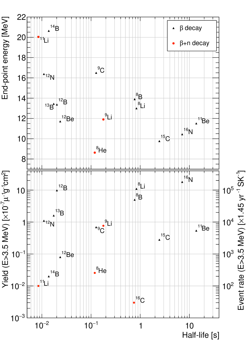
Figure 2: The half-lives, endpoint energies, and yields of $\beta$ decays of expected radioisotopes produced by oxygen nucleus spallation from cosmic ray muons. The yields are taken from Li & Beacom (2014), and the yields for these isotopes account for the fraction of neutrons accompanying the channel. Event rates are calculated considering the average muon rate ($\sim 2~\rm Hz$) and average track length ($\sim 2300~\rm cm$).

Radioisotopes shown with red markers in Figure 2 represent those that have a $\beta+n$ decay branch, such as $\rm{}^{11}Li$, $\rm{}^{15}C$, $\rm{}^{8}He$, and $\rm{}^{9}Li$ in this case. $\rm{}^{11}Li$ has a short half-life, which can be easily removed using time correlation with the parent muon. In addition, the yield of $\rm{}^{11}Li$ is expected to be rather small compared to other spallation isotopes; thus, the contribution of $\rm{}^{11}Li$ can be neglected. Similarly, the $\rm{}^{16}C$ yield is quite small and the endpoint energy of the $\rm{}^{16}C$ $\beta+n$ decay channel is approximately 5.5 MeV, which falls outside the range of Figure 2; therefore, this is negligible in this analysis. Furthermore, $\rm{}^{8}He$ is a subdominant component due to the low yield compared to $\rm{}^{9}Li$.

In contrast, $\rm{}^{9}Li$ has a relatively long half-life (0.178 s) and has a high yield compared to other isotopes. The total yield of $\rm{}^{9}Li$ is $0.76\times 10^{-7}~\mu^{-1}~{\rm g}^{-1}~{\rm cm}^{2}$ above 3.5 MeV, with a sufficiently high end-point energy to contaminate the DSNB signal energy window. Therefore, $\rm{}^{9}Li$ forms a non-negligible background even after neutron tagging in this analysis.

Although liquid-scintillator experiment measurements have demonstrated better agreement with theory (Abe et al., 2023; An et al., 2024), the predicted yields of spallation isotopes from oxygen are still inconsistent with measurements; as Zhang et al. (2016) showed, the measured yield in SK is smaller than the expectation in Li & Beacom (2014) by a factor of 3.1–4.7. This indicates that there is still a limited understanding of the composition of radioisotope production. Thus, we employ yield measurement results in our analysis.

3.4 Reactor Neutrinos

Electron antineutrinos created in nearby reactors irradiate SK. Then, these neutrinos undergo IBD interaction and mimic DSNB signals because they have the same signature. While we know the precise locations of these reactors, the directional information carried by neutrinos is mostly lost through IBD (Vogel & Beacom, 1999). The flux estimations of these reactor neutrino events are performed by SKReact (2023) based on the reactor neutrino model of Baldoncini et al. (2015). This calculation takes into account Japanese reactor activities during the SK-Gd observation period, along with neutrino oscillations due to the distance from reactors. This flux at SK is predicted up to $E_{\nu}=9.3~\rm MeV$. Figure 3 shows the expected reactor neutrino event spectra during the SK-VI period as functions of both true and reconstructed kinetic energy, along with the DSNB flux example. We can see that the reactor neutrinos constitute a significant contribution to the DSNB signal. In the signal window, energy resolution effects are what primarily determine the contribution of reactor neutrino events.

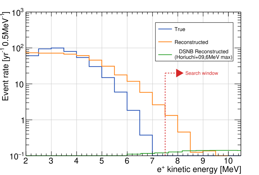
Figure 3: Positron kinetic energy of predicted reactor neutrino IBD events. An example of the DSNB flux is also shown as well. The vertical axis shows the average event rate per year. The variation of the operating period of Japanese reactors is averaged into the IBD event creation rate.

3.5 Solar Neutrinos

The production chain of heavier elements in the Sun’s core leads to the decay of ${}^{8}\text{B}\to{}^{8}\text{Be}^{*}+e^{+}+\nu_{e}$. For any neutrino flavor, electron elastic scattering through $\nu(\bar{\nu})+e^{-}\to\nu(\bar{\nu})+e^{-}$ off free electrons in SK will generate a prompt event, and the energy enters the DSNB search region. Luckily, the following two features of this scattering make solar neutrinos an easily reducible background: First, since no neutrons are produced, neutron tagging will largely remove these events. Second, for samples without a neutron tagging requirement, we can still exploit the strong correlation between the reconstructed electron direction and the direction toward the Sun due to the forward-scattering nature of electrons (Abe et al., 2021, 2024b).

4 Event selection

This analysis searches for IBD events, characterized by the temporal and spatial coincidence of a prompt positron event and a delayed neutron event, resulting from thermal neutron capture on Gd or hydrogen nuclei. We apply a series of event selection criteria to observed data from the SK-VI and SK-VII periods associated with an SHE trigger and a subsequent AFT trigger when available. The lower energy threshold of the analysis region is set to $E_{\rm rec}=7.5$ MeV due to the sufficient SHE trigger efficiency at this energy and the negligible amount of reactor neutrino background events (see Section 3.4). The upper energy bound of the DSNB signal region of interest depends on the analysis method described later.

The following sections describe four stages of event selections: primary noise reduction (Section 4.1), spallation event reduction (Section 4.2), atmospheric neutrino event reduction (Section 4.3), and delayed neutron identification (Section 4.4).

4.1 Basic Noise and Low-Quality Event Reduction

We first select the SHE-triggered events without OD triggers, and pair them with a subsequent AFT window when available. As noted in Section 2 and Table 1, the AFT trigger rate varies depending on the detector phase. Next, the collected events with $E_{\rm rec}$ below 79.5 MeV undergo a set of cleaning cuts to remove events from PMT noise, radioactivity from the detector wall, and cosmic-ray muon activity. In particular, the candidate events are required to have a reconstructed vertex 2 m or more inside the ID wall to avoid radioactive backgrounds and poorer reconstruction performance. This defines a fiducial volume of 22,500 $\rm m^{3}$. To further remove backgrounds originating from the detector walls without shrinking the fiducial volume, we impose an energy-dependent “effective” distance criterion. This distance is calculated from the wall to the reconstructed vertex along the axis defined by the reconstructed event direction. In addition, we exclude events that occur within $50~\rm\mu s$ of high-charge events, defined as those with a total charge deposited on PMTs exceeding 500 p.e. equivalent. This cut rejects events activated by cosmic-ray muons, including decay electrons and nuclear events that occur rapidly following muon interactions. Finally, we apply a vertex reconstruction quality cut to remove non-electron-like noise events based on the PMT hit timing distributions per event. The inefficiency associated with this quality cut is below 1%, as validated by the IBD signal MC simulation. Events that pass these reduction criteria are hereafter referred to as DSNB candidates.

4.2 Spallation Reduction

We utilize timing and spatial correlations between DSNB candidates and cosmic ray muons to remove the spallation background, called “spallation cuts.” In this analysis, a data-driven study is conducted to reduce the spallation background. Given that the maximum endpoint energies of the electrons or positrons are about 20.5 MeV, spallation event reduction algorithms are applied up to $E_{\rm rec}=23.5$ MeV, taking into consideration energy resolution effects. The overall concept of this reduction is the same as that of previous SK analyses (Abe et al., 2021; Harada et al., 2023), which consists of some pre-treatment cuts, a detailed likelihood approach, and a robust cut for high-energy spallation.

One notable improvement from previous work (Abe et al., 2021) is that the shower neutrons from muon interactions are now identified by the Gd capture signal, as measured by Shinoki et al. (2023). It has become possible to efficiently identify muons that are likely to cause hadronic showers, i.e., spallation. The timing between DSNB candidates and muons causing a neutron shower, along with spatial correlations between DSNB candidates and the neutron shower, is employed to remove such background events. More details of these “neutron cloud cut” criteria and other pre-treatments are described in Appendix A. Other steps for reducing the spallation events exactly follow those of previous searches (Abe et al., 2021; Harada et al., 2023).

4.3 Atmospheric Neutrino Reduction

To reduce atmospheric neutrino backgrounds, we employ the same event selection steps as in previous searches (Abe et al., 2021; Harada et al., 2023). These make use of the reconstructed Cherenkov angle ($\theta_{c}$), the PMT activity before the main PMT hit peak from the prompt signal, the reconstructed particle decays after this peak, the clearness of the PMT hit pattern,

$$L_{\rm clear}=\frac{N_{\rm triplets}(\theta_{c}\pm 3^{\circ})}{N_{\rm triplets}(\theta_{c}\pm 10^{\circ})},$$ (2)

where the number of hit PMT triplets $N_{\rm triplets}$ are counted that give a Cherenkov angle within a given difference from the overall Cherenkov angle $\theta_{c}$, and the average charge deposited per PMT hit.

In addition, a new atmospheric neutrino background reduction step is introduced in this analysis to target NCQE events. These and certain CCQE processes can produce secondary $\gamma$-emission on the timescale of the initial knock-out nucleon thermalization. Since this thermalization is fast enough to be contained within the SHE prompt trigger window, PMT hits from the initial NCQE interaction and secondary $\gamma$-emission are collected together. The multiple $\gamma$-emission then leads to multiple Cherenkov cones in the prompt event, and the total prompt energy can easily exceed 10 MeV. Furthermore, a varying number of neutrons can be produced in the final state due to the secondary interactions of the initial knock-out nucleon.

In past analyses (Abe et al., 2021; Harada et al., 2023), NCQE backgrounds were targeted in one of two main ways. The first was through the reconstructed Cherenkov angle ($\theta_{c}$) selection, and the second was the number of neutrons observed after the candidate prompt event. As first introduced by Malek et al. (2003), the reconstructed Cherenkov angle of multi-cone prompt events tends to have a large $\theta_{c}$ compared to the single electron-like event due to the hit pattern, as illustrated in Figure 4. Thus, events whose $\theta_{c}$ value is significantly larger than $42^{\circ}$ can be rejected as NCQE events. Next, the requirement of identifying a single neutron capture in the final state removes many NCQE events because NCQE interactions can have neutron multiplicities different from one. With these two methods, the NCQE remaining rate was reduced to below 10%, but more NCQE events were still present compared to nominal DSNB predictions. If multiple Cherenkov cones in a prompt event point in similar directions, the reconstructed Cherenkov angle cannot distinguish the hit pattern from that of a single Cherenkov cone.

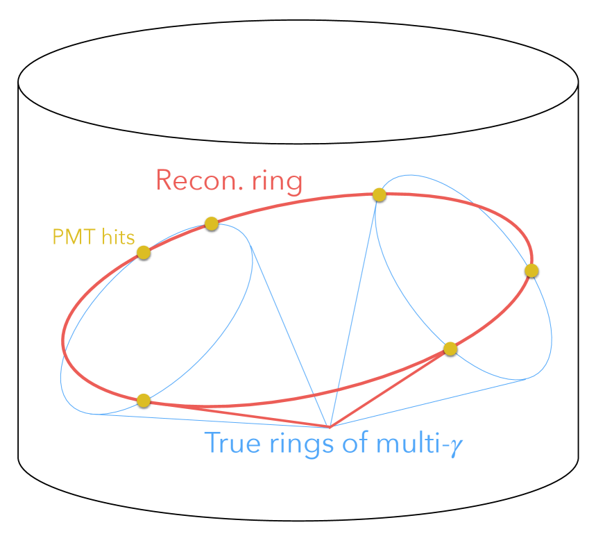
Figure 4: Illustration of a single event with multiple Cherenkov cones. The reconstructed $\theta_{c}$ appears to have a larger angle.

A new reduction variable is introduced for further reducing NCQE backgrounds, termed the “multiple scattering goodness” (MSG) variable. In the context of the DSNB search, this variable was first introduced by Bays et al. (2012) to quantify the multiple Coulomb scattering of electrons, thereby reducing solar neutrino backgrounds. Since multiple Coulomb scattering limits the directional resolution of non-showering electrons, MSG provides a measure of angular resolution. It is also capable of distinguishing multi-$\gamma$ events from single-$e^{\pm}$ events more explicitly. Instead of being sensitive to the overall PMT pattern for $\theta_{c}$, the MSG variable is sensitive to the substructure of the PMT hits. The main steps for calculating MSG are shown in Figure 5.

For each event, this algorithm identifies cones with $42^{\circ}$ opening angle originating from the reconstructed prompt vertex that could explain the PMT hit pattern. The axis of each candidate cone defines a unit vector $\vec{u}_{i}$ that points in the direction of the cone. The value of MSG is the magnitude of the sum of the axis unit vectors in the largest cone cluster divided by the total number $N_{\rm cones}$ of candidate cones, or

$${\rm MSG}=\frac{1}{N_{\rm cones}}\left|\sum_{i\in{\rm cluster}}\vec{u}_{i}\right|.$$ (3)

The largest cluster is taken as the most candidate cones whose edges fit within a broader cone of $50^{\circ}$ opening angle.

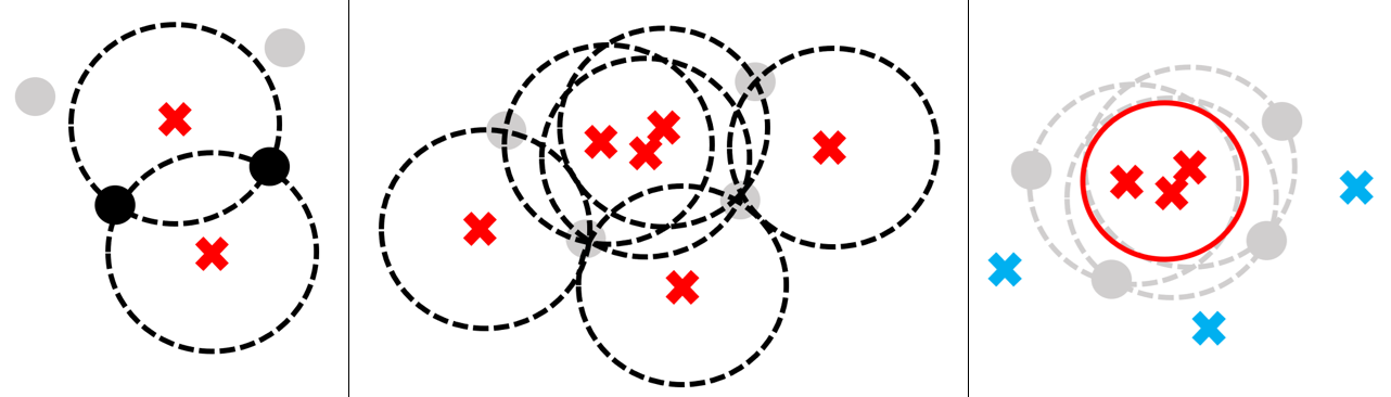
Figure 5: Main steps for calculating MSG. (Left) Start with one pair of PMT hits (black dots). With origin at the reconstructed prompt vertex, define any cones with axis (red cross) and $42^{\circ}$ opening angle whose edges (black, dashed) coincide with both PMT hits. (Middle) Iterate through every possible pair of PMT hits. After this, each PMT hit pair will have zero, one, or two candidate cones. (Right) Identify the largest cluster of candidate cones, defined as those whose axes fit within $28.4^{\circ}$ of a single direction (red, solid). Axes in the cluster are kept in red, while those outside the cluster are changed to blue. Clustering is done in multiple iterations to maximize the magnitude of the sum of the largest cluster’s axis vectors. MSG is defined as this magnitude divided by the total number of candidate cones.

As shown in Figure 6, there is a population of NCQE events in the signal-like $\theta_{c}$ region around $42^{\circ}$, whereas these can be reduced by introducing MSG cut criteria. Smaller MSG values indicate that multiple cones are more likely, while larger values suggest the presence of a single cone, as shown in the top panel of Figure 7. The event selection using MSG further distinguishes DSNB signals from NCQE background events beyond the conventional $\theta_{c}$ event selection, as shown by the Receiver Operating Characteristic (ROC) curve in the bottom panel of Figure 7.

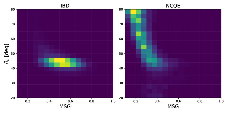
Figure 6: Cherenkov angle versus MSG for IBD and NCQE events for $E_{\text{rec}}\in[11.5,23.5]$ MeV. As the angle between multiple $\gamma$’s decreases for NCQE events, the MSG value increases. In the characteristic $\theta_{c}$ region for IBD signals, the NCQE MSG values are, on average, lower than those of IBD.

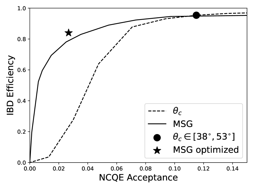
Figure 7: MSG distributions for atmospheric neutrino backgrounds and IBD signal events (amplified by a factor of 100) for $E_{\text{rec}}\in[11.5,23.5]$ MeV (top). ROC curves for MSG-only and $\theta_{c}$-only reduction with an old $\theta_{c}$ working point and MSG working point for $E_{\text{rec}}\in[11.5,23.5]$ MeV as optimized in Section 5 in 2 MeV bins for $E_{\text{rec}}\in[11.5,23.5]$ MeV (bottom). Note that the MSG ROC curve shown is defined with a global MSG threshold over the whole energy range, which leads to an offset in the MSG optimized point.

4.4 Neutron Tagging

As described in Section 2, SHE and subsequent AFT triggers record PMT hits within $[-5,~535]~\mu$s from the SHE trigger time. We can search offline for a hit cluster originating from a neutron capture and classify the prompt event based on the number of tagged neutrons. In this analysis, we require exactly one tagged neutron to identify the event as an IBD event. Previous DSNB searches in SK used a Boosted Decision Tree (BDT) for neutron detection in pure water (Abe et al., 2021), as well as a box cut-based neutron capture selection in the first Gd-loaded phase (Harada et al., 2023). In this study, we retrained the BDT to include neutron captures on Gd and independently developed a Neural Network (NN) for neutron identification. DSNB search results using both approaches are discussed in the following sections, including the cross-validation of their performances and physics inferences. Both neutron detection approaches include a pre-selection that requires hit clusters above a certain threshold in a given timing window, where the time-of-flight from the reconstructed prompt vertex to each PMT is subtracted. These threshold criteria are defined as seven or more hits in 14 ns for the NN and as five or more hits in 10 ns for the BDT. Feature variables and an output score for both the NN and BDT are calculated for each hit cluster to judge whether the hit cluster is a neutron signal. The neutron detection efficiency $\epsilon_{n}$ is determined by $\epsilon_{\rm pre}\times\epsilon_{\rm score}$, where the $\epsilon_{\rm pre}$ represents the efficiency that the pre-selection picks a neutron, and $\epsilon_{\rm score}$ is the selection efficiency by the output score of both neutron identification tools.

The NN employs 12 variables representing the number of PMT hits, spatial features of PMT hits, the RMS of the hit timing peak, and the distance from the ID wall. These are calculated for each candidate searched from the window $[4,535]~\rm\mu s$. Details about variables and optimization are described in Appendix C.

The BDT takes in 22 variables related to the spatial topology of the PMT hits, their timing distributions, and the charge deposited. In SK-IV, the neutron search window for the BDT sample began at 14 $\mu$s after the SHE-triggered timing, whereas it is placed at 2 $\mu$s in SK-Gd, as neutron captures happen faster due to Gd-loading. Further information on BDT neutron identification inputs can be found in Appendix D, and details about the training of the algorithm are provided by Giampaolo (2023).

Both neutron identification approaches explore neutron-like clusters based on the NN/BDT output and count up the number of neutrons ($N_{\rm n}$) for each prompt DSNB candidate. Figure 8 shows the averaged neutron detection efficiency and misidentification probability as the output score threshold is varied for both NN/BDT. A comparison to the SK-IV pure-water BDT performance is included. We can see the curve is significantly improved compared to the pure-water case, owing to the enhanced neutron signal by Gd.

Figure 8: Neutron detection efficiency $\epsilon_{\rm score}$ and misidentification probability of noise candidate. The $\epsilon_{\rm pre}$ for NN (BDT) are 75.0% (77.2%) for SK-VI and 85.1% (87.3%) for SK-VII. The number of noise candidates per event after pre-selection, averaged over the entire periods, is 47 for SK-VI and 58 for SK-VII, respectively.

4.5 Validation of Event Selection

4.5.1 Calibration Samples

Before applying the full event selection to all data (i.e., “unblinding”), we define validation steps to verify our event reduction for both signal- and background-like events. Some of these are entirely new procedures to the SK DSNB search. We begin with data from the LINear ACcelerator (LINAC) calibration (Nakahata et al., 1999) and then focus on the calibration using the radioactive source Americium-Beryllium (Am/Be) (Abe et al., 2022a). We focus on validating the overall agreement between the observable distributions of data and MC simulations, while also defining systematic uncertainties arising from event reduction steps. The LINAC monochromatic electron events behave similarly to the IBD prompt signal from the DSNB. The Am/Be source emits neutrons, and these events are analogous to those of IBD because the neutron behavior in source energies is similar to that of IBD neutrons. Comparing these calibration data and MC, we can validate the effects of atmospheric neutrino background reduction (Section 4.3) and subsequent neutron tagging (Section 4.4) on the IBD signal.

After verifying that the LINAC data distributions closely match those of the MC, the associated uncertainties on the IBD signal efficiency for each reduction are estimated. We compare the selection efficiency of data ($\epsilon_{\rm data}$) and MC ($\epsilon_{\rm MC}$) and define the relative 1$\sigma$ uncertainty of each reduction step as $(\epsilon_{\rm MC}-\epsilon_{\rm data})/\epsilon_{\rm data}$.

In a similar procedure with Am/Be calibration data for both NN and BDT algorithms, we estimate the systematic uncertainty on the neutron detection efficiency. As a function of either algorithm’s cut point and the various calibration configurations, we take the difference in predicted and observed tagging efficiency as the 1$\sigma$ systematic uncertainty. Appendix E details the comparison of Am/Be calibration data with MC samples.

4.5.2 Background Samples

The remaining steps before unblinding include exploiting background-dominated samples. First, we consider the NCQE background behavior. A dedicated SK-Gd study on atmospheric NCQE interaction modeling followed the event selection used in SK DSNB searches (Sakai et al., 2024). With a Cherenkov angle selection of $\theta_{c}$ above $50^{\circ}$, it was demonstrated that the predicted $\theta_{c}$, energy, and neutron multiplicity distributions agree well with data.

Next, for data with $E_{\rm rec}>29.5~\rm MeV$, we apply all reduction criteria since we assume a comparatively negligible DSNB contribution based on a wide range of theoretical DSNB models. These events are dominated by atmospheric neutrino CC backgrounds, notably the decays of invisible muons and pions, categorized as part of the “non-NCQE” backgrounds (Section 3.2). Since this background contributes significantly to the DSNB signal region, this sample helps validate the scaling of remaining atmospheric background predictions in the adjacent signal region.

Table 2 presents a summary of these validation steps. Once all of them are performed while demonstrating good data/MC agreement, we proceed to unblind the full dataset with all reduction criteria applied. This includes preparing the final samples for both the spectrum-independent and spectrum-dependent searches. These two statistical approaches are done in parallel, and we detail their procedures and results in the following sections.

Table 2: Validation samples ahead of data unblinding.

Sample	Item Checked
LINAC	IBD prompt signal
Am/Be	IBD delayed signal (Appendix E)
$\theta_{c}\in[50^{\circ},~90^{\circ}]$ sample	Atm. NCQE (See Sakai et al. (2024))
$[29.5,79.5]$ MeV sample	Scaling of Atm. non-NCQE (Section 5.1)

5 DSNB Spectrum-independent electron antineutrino search

In this section, we describe the search for electron antineutrino IBD events over the expected backgrounds on a bin-by-bin basis. This search makes no explicit assumptions about the theoretical model of the IBD signal, ensuring that the result can be applied to any astrophysical electron antineutrino flux. The upper energy bound of the signal region is set to $E_{\rm rec}<29.5$ MeV due to a low expected DSNB flux and increasing atmospheric neutrino background at higher energies. First, we discuss the backgrounds that should be taken into account in this analysis, cut optimization, and the resulting signal efficiency. Then, after estimating the systematic uncertainties of the backgrounds, we introduce the final search result.

5.1 Scaling of Atmospheric Non-NCQE Background

Events with $E_{\rm rec}=29.5-79.5~\rm MeV$ are utilized as the validation sample for the atmospheric non-NCQE background, as mentioned in Section 4.5. We start with the same procedure as Abe et al. (2021); Harada et al. (2023), which determines non-NCQE normalization by comparing $E_{\rm rec}$ distributions between data and MC in this high-energy sideband region. To get accurate estimations, we compared the $E_{\rm rec}$ distribution without the neutron tagging step for the SK-VI sample. In SK-VII, we get more neutron detection efficiency, so a loosened neutron selection is applied to obtain statistics before comparison.

5.2 Accidental Coincidences

With our MC samples, we can predict the remaining events of nearly all event categories after neutron tagging. Additionally, we should estimate instances where a coincidence between a prompt event and a misidentified delayed signal in our neutron search algorithm occurs, referred to as “accidental coincidences.” A significant contribution to accidental coincidences comes from spallation isotopes, since we do not fully simulate the spallation background yield due to the large uncertainties in isotope production. Furthermore, we do not simulate solar neutrino events. Thus, we evaluate the accidental background events in a data-driven way.

We first apply all reduction steps except for neutron tagging to the unblinded full dataset, which is divided into 2 MeV energy bins. From the misidentification rate $f_{\text{mis}}$ shown in Figure 8, we estimate the number of accidental coincidence background events $B_{\text{acc}}$ as

$$B_{\text{acc}}=f_{\text{mis}}\times N_{i},$$ (4)

where $N_{i}$ is the number of events before neutron tagging in each energy bin $i$.

5.3 Cut Optimization

This section describes the optimization for the spallation cut, atmospheric neutrino event reduction, and neutron identification. The energy binning is selected to 2 MeV, chosen to match the SK energy resolution at $\mathcal{O}(10)$ MeV.

5.3.1 Spallation Cut

The optimization scheme is identical to that of Abe et al. (2021), which computes the working point of the spallation likelihood cut threshold specified in Section 4.2, to maximize sensitivities using the Rolke method (Rolke et al., 2005) under the null signal assumption. The working points are determined by taking into account all backgrounds, including $\rm{}^{9}Li$, accidental background, and all other types of backgrounds that remain after applying the optimal NN neutron tagging cut. Above 16 MeV, there are insufficient event statistics to fine-tune the cut criteria. Therefore, the cut point is chosen to maximize signal efficiency as we expect minimal contribution from the remaining spallation background in this energy region.

5.3.2 Positron Event Selection

The reduction criteria targeting atmospheric neutrinos are determined by comparing atmospheric and IBD signal MC predictions in each 2 MeV $E_{\rm rec}$ bin because the distributions of these values for signal and background events vary with energy. The figure of merit used in the optimization steps is taken to be $S/\sqrt{(S+B)}$.

Given the strong correlation between the Cherenkov angle and MSG observables, these two reduction steps are optimized together. The Cherenkov angle selection is optimized to be a tight interval that rejects visible $\mu$/$\pi$ events at low values and NCQE backgrounds at high values, while the MSG selection is set to a minimum threshold to reject multi-cone events. More comments about final NCQE background contamination levels from these cuts are discussed in Appendix B.

Finally, high ring clearness and high charge-per-hit indicate Cherenkov-visible $\mu/\pi$-like events. An upper bound for these parameters is optimized to remove such events from the final sample.

5.3.3 Neutron Identification

The spectrum-independent DSNB search is performed separately using both the NN-based and BDT-based neutron identification to allow cross-comparison. For this analysis, neutron identification criteria for both methods were chosen to ensure that the two methods have similar misidentification rates.

For the NN-based approach, we select the cut value of the NN score such that the $f_{\rm mis}$ satisfies an expected misidentification rate of 0.02% per prompt event with the assumption of $f_{\rm mis}$ being independent of the prompt event energy. The search time window is optimized to maximize the signal-to-noise ratio, resulting in the $[4,535]~\rm\mu s$ for SK-VI and $[4,270]~\rm\mu s$ for SK-VII, respectively. More details are given in Appendix C.

For the BDT-based approach, the neutron selection criteria are determined in bins of 2 MeV, considering the rates of atmospheric neutrino MC, accidental coincidences, and IBD MC predictions. We also apply a stricter selection to each candidate using three characteristic variables: the reconstructed Cherenkov photon count, the number of PMT hits in clusters of three, and total number of PMT hits for the neutron candidate (see Appendix D for more details).

Figure 9 shows the neutron tagging performance in the form of signal efficiency against the background misidentification rate for NN and BDT. In the plot, we adopt two performance metrics that are directly related to the final samples requiring $N_{\rm n}=1$. First, the signal efficiency in Figure 9 represents the probability of an IBD event to satisfy the $N_{\rm n}=1$ condition. The misidentification rate $f_{\rm mis}$ is explained in Section 5.2. Loosening the cut criteria will increase signal efficiency but also lead to more misidentification. Eventually, with sufficiently loose criteria, we will more frequently mistake backgrounds as neutrons, which causes $N_{\rm n}>1$ and, therefore, decreases IBD efficiency by our definition.

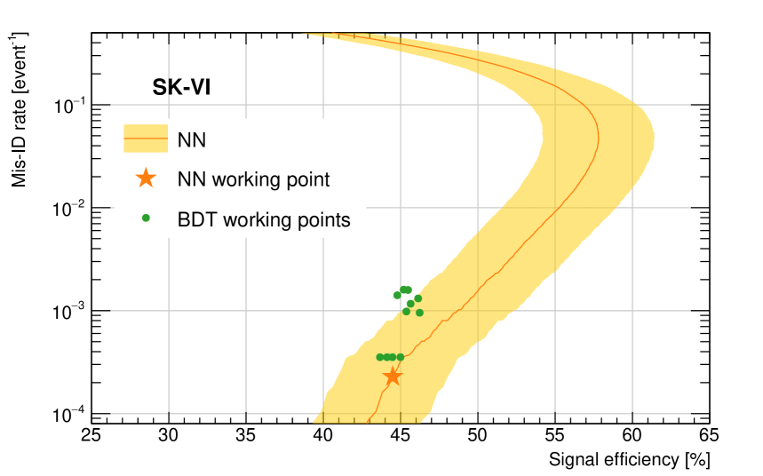
Figure 9: Signal efficiency of neutron tagging and misidentification rate for the NN (Orange, solid line) and BDT (Green, circles) with strict pre-cut, respectively. The signal efficiency represents the probability of an IBD event to satisfy the $N_{\rm n}=1$ condition. The error band representing the uncertainty in signal efficiency is evaluated by the agreement of the MC sample with the calibration data (See Appendix E).

5.4 Signal Efficiency of Final Sample

Figure 10 shows the IBD signal efficiency for each 2 MeV $E_{\rm rec}$ bin after applying each optimized signal selection criterion for SK-VI and SK-VII, respectively. The final IBD signal efficiency is shown for both the NN-based and BDT-based methods for comparison. These final efficiencies are also summarized in Table 3. The efficiencies before neutron tagging are comparable between SK-VI and SK-VII, whereas the neutron tagging effect on the final efficiencies increases markedly in SK-VII compared to SK-VI. Systematic uncertainties on the signal efficiency for each reduction are summarized in Table 4.

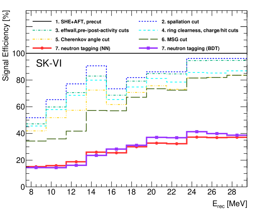
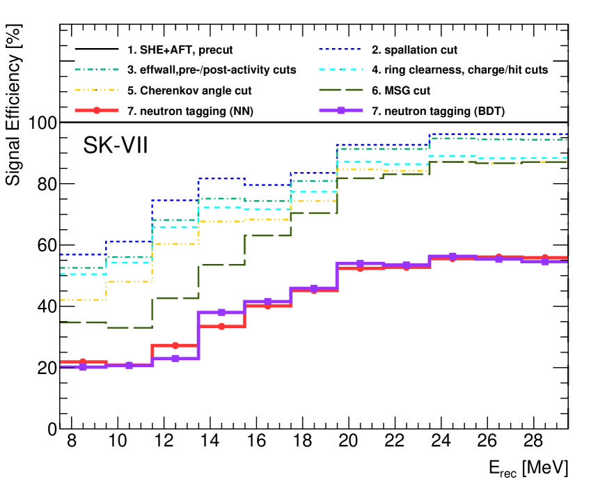
Figure 10: DSNB signal efficiencies for the signal energy region, for SK-VI (top) and SK-VII (bottom), normalized after the trigger requirement and basic noise reductions. Each line shows the cumulative efficiency at each stage, performed in the order shown in the legend. Red (purple) with circle (square) points show the final efficiency after NN (BDT)-based neutron tagging.

Table 3: Signal efficiency after applying all reductions, including both NN and BDT-based neutron tagging, for each 2-MeV $E_{\rm rec}$ bin in the signal energy region.

$E_{\rm rec}$ [MeV]	Signal efficiency[%]
	SK-VI		SK-VII
	NN	BDT	NN	BDT
7.49 - 9.49	15.1%	14.4%	21.9%	20.2%
9.49 - 11.5	15.9%	14.4%	20.8%	20.7%
11.5 - 13.5	18.8%	16.2%	27.2%	23.0%
13.5 - 15.5	26.0%	23.6%	33.4%	38.0%
15.5 - 17.5	25.5%	28.3%	40.1%	41.6%
17.5 - 19.5	30.0%	31.1%	45.2%	45.9%
19.5 - 21.5	32.8%	37.1%	52.4%	54.0%
21.5 - 23.5	32.3%	36.8%	52.7%	53.5%
23.5 - 25.5	37.2%	41.3%	55.5%	56.3%
25.5 - 27.5	36.9%	39.9%	56.1%	55.4%
27.5 - 29.5	37.1%	38.7%	55.8%	54.6%

Table 4: Systematic uncertainties on the signal efficiency from background reduction, calculated as described in Section 4.5.

	Relative systematic error
Cut	SK-VI	SK-VII
$q_{50}/n_{50}$ cut	0.20%	0.25%
$\theta_{\rm C}$ cut	1.3%	0.94%
MSG cut	1.7%	1.4%
Neutron tagging (NN/BDT)	8.4%/5.0%	3.4%/6.0%

5.5 Uncertainties on Background Estimation

This section presents the systematic uncertainties corresponding to each background component. In the present analysis, we evaluated uncertainties related to the MSG cut and updated the uncertainties for atmospheric non-NCQE events and neutron tagging. Table 5 summarizes the relative systematic uncertainties assigned to each background category.

5.5.1 Atmospheric NCQE Background

In light of the new MSG cut, we update the uncertainty from the previous SK analyses (Abe et al., 2021; Harada et al., 2023) on the remaining NCQE level. This is accomplished by an MC-driven estimate. In particular, we examine the difference in the reduction efficiency between two distinct MC models. As discussed in Section 3.2, knock-out nucleons from NCQE interactions are energetic enough to partake in secondary interactions with other nuclei to produce secondary $\gamma$-emission. The way in which these “nuclear cascades” occur impacts the multi-cone behavior of NCQE events and, therefore, MSG reduction. A discussion of nuclear cascade modeling and NCQE events was performed by Abe et al. (2025). For these reasons, we generate one sample with the INCL model and another with the BERT model. The BERT model shows the most discrepant results from INCL in some validation results Hino et al. (2025); Sakai et al. (2024), such that it should provide a reliable estimate of the maximal difference in MSG cut efficiency between all possible models. Based on the discrepancy of the NCQE predicted remaining rate using the BERT and INCL models, we conservatively estimate 20% as the additional uncertainty in the level of remaining NCQE backgrounds, independent of energy. Other uncertainties on the atmospheric neutrino flux and NCQE cross-section are assumed to be the same as previous SK analyses (Abe et al., 2021; Harada et al., 2023), which were estimated to be $\pm 68\%$. In total, the new uncertainty for the remaining atmospheric neutrino NCQE background is estimated as $\pm 71\%$ by combination with the additional $\pm 20\%$ uncertainty in quadrature.

5.5.2 Atmospheric Non-NCQE Background

The overall systematic uncertainty on the flux of atmospheric neutrinos and the cross-section for non-NCQE interactions are determined by the same procedure as in Section 5.1. This is an energy-binned fit of sideband MC to the data for which we extract a $\pm 1\sigma$ uncertainty. In SK-VI, since this fit is performed before neutron tagging, we add a 30% systematic uncertainty on the neutron multiplicity of atmospheric neutrino interactions in quadrature, as in Harada et al. (2023). Then, the resulting systematic uncertainties are $\pm 36\%$ for SK-VI and $\pm 41\%$ for SK-VII.

5.5.3 Lithium-9 Background

Below 16 MeV, most of the background from spallation after neutron tagging consists of $\rm{}^{9}Li$ ($\beta+n$) decays. The normalization is taken from Zhang et al. (2016), which measured a yield of $0.86\pm 0.12\,(\mathrm{stat.})\pm 0.15\,(\mathrm{sys.})$ ${\rm kton^{-1}\cdot day^{-1}}$ in SK. The systematic uncertainty on the scaling is 22% in yield uncertainty, taken from Zhang et al. (2016). Additionally, according to Abe et al. (2021), there is approximately a 50% uncertainty in our data-driven estimation of the $\rm{}^{9}Li$ remaining rate after spallation cuts. Uncertainties related to the reduction steps other than the spallation cut, primarily from neutron tagging, are summed in quadrature to the systematic uncertainty estimate, resulting in a total of $\pm 55\%$.

5.5.4 Reactor Neutrinos

The reactor neutrino background is estimated by scaling the IBD simulation following the reactor neutrino flux introduced in Section 3.4. These events populate only the lowest energy bin, ranging from $7.5-9.5$ MeV, as shown in Figure 11. The flux strongly depends on the activity of each reactor. In this analysis, we conservatively assign a $\pm 100\%$ systematic uncertainty on the reactor neutrino events.

5.5.5 Accidental Coincidence Background

For the accidental coincidence background, the uncertainty on $f_{\rm mis}$ from Equation 4 should be considered. Since we evaluate $f_{\rm mis}$ by real detector noise, the statistical uncertainty of $f_{\rm mis}$ at a given algorithm’s working point over the entire period is assigned as the total uncertainty, which is approximately $\pm 5\%$ for both SK-VI and SK-VII.

Table 5: Systematic uncertainties on background predictions for the spectrum-independent electron antineutrino search.

	Relative systematic error
Event category	SK-VI	SK-VII
Atmospheric-$\nu$ (NCQE)	$\pm 71\%$	$\pm 71\%$
Atmospheric-$\nu$ (non-NCQE)	$\pm 36\%$	$\pm 41\%$
Spallation 9Li	$\pm 55\%$	$\pm 55\%$
Reactor-$\nu$	$\pm 100\%$	$\pm 100\%$
Accidental coincidence	$\pm 5\%$	$\pm 5\%$

5.6 Results

5.6.1 Final Data Samples

Data are divided into pre-determined energy bins as done by Harada et al. (2023), for which the first two ($E_{\rm rec}=7.5-9.5$, $9.5-11.5$ MeV) are spallation ⁹Li-dominated, and the next three ($E_{\rm rec}=11.5-15.5$, $15.5-23.5$, $23.5-29.5$ MeV) contain the lowest background levels. In particular, the third bin contains the high-energy tail of $\rm{}^{9}Li$ events, while non-NCQE backgrounds start to dominate in the fourth bin. Finally, in the fifth bin, almost all events are non-NCQE events. The remaining bins ($E_{\rm rec}=29.5-79.5$ MeV divided into 10 MeV intervals) form the high-energy sideband. The final energy spectra after all reduction criteria are applied using either NN or BDT for neutron tagging are shown in Figure 11. Again, the only difference in the two samples shown is the neutron tagging algorithm applied.

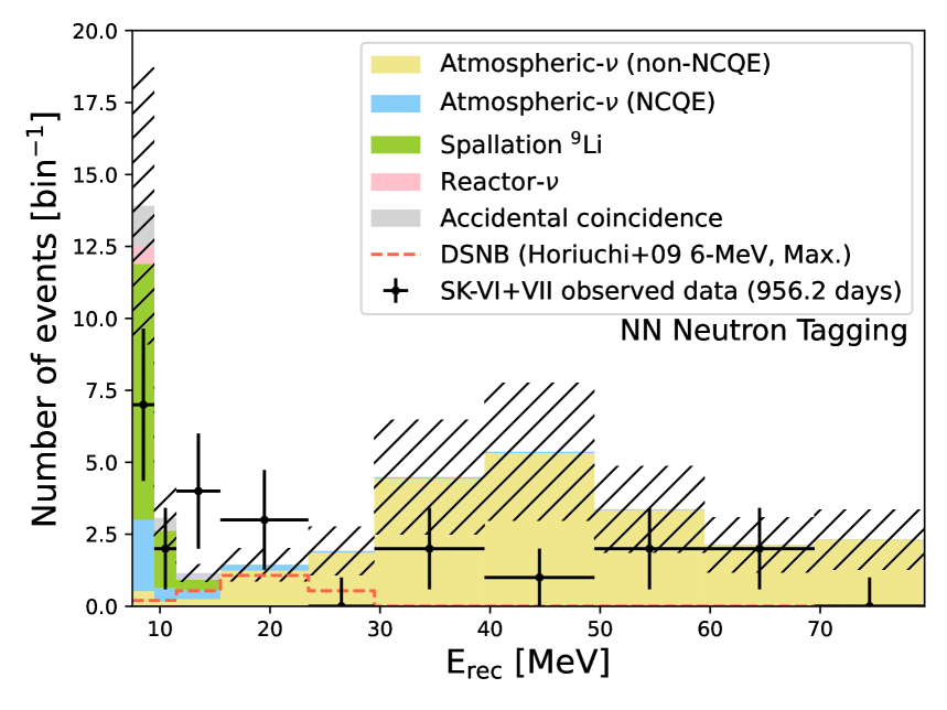
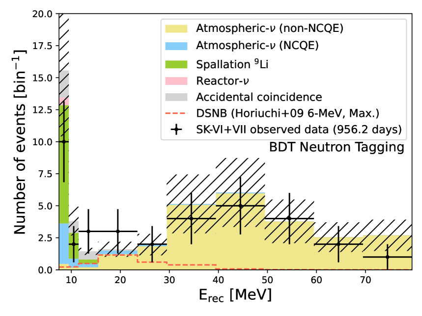
Figure 11: Reconstructed positron equivalent kinetic energy spectra of the data and the expected background after all reductions, including the requirement of $N_{\rm n}=1$, for NN (top) and BDT (bottom) neutron tagging. The error bars in the data points represent the statistical error value estimated by taking the square root of the number of observed events. Color-filled histograms show the expected backgrounds, which are stacked on top of each other. The hatched areas filled onto the stacked background histograms represent the total absolute background systematic uncertainty for each bin. The signal search window is $E_{\rm rec}\in[7.5,~29.5]$ MeV. For illustrative purposes, a typical DSNB expectation from optimistic values of Horiuchi et al. (2009) is drawn separately from the background histograms as a red-dashed (bottom) line, superimposed.

In each energy bin, we generate a probability distribution for the total event count under a background-only hypothesis. This is achieved by performing pseudo-experiments based on the expected value of each background category, varied according to its associated systematic uncertainty, assuming Gaussian distributions. From these distributions, a background-only p-value, $p_{b}$, is calculated using the observed number of events from the data. For both NN and BDT final samples, we conclude that no significant excess is observed over the background, while the smallest $p$-value is 0.08.

5.6.2 Astrophysical Electron Antineutrino Flux Upper Limit

With no significant excess, we then place upper limits on the astrophysical $\bar{\nu}_{e}$ flux per energy bin. We adopt the CL_s approach (Read, 2002), for which a background-plus-signal p-value $p_{s+b}$ is modified by the rejection coming from the background-only hypothesis with $p$-value $p_{b}$ giving:

$$\text{CL}_{s}\equiv\frac{p_{s+b}}{1-p_{b}}\leq\alpha.$$ (5)

This method is well suited when we expect an observation to be statistically consistent with both background-only and signal-plus-background hypotheses—especially when the signal is unknown—since $p_{s+b}$ is increased when $p_{b}$ is also large.

Both expected and observed upper limits are calculated per energy bin at 90% CL_s, for which $\alpha=0.1$. For the expected limit, $p_{b}$ is determined by the background-only expectation value of the number of events in that bin. In the case of the observed limit, $p_{b}$ is determined by the observed number of events per bin. For both scenarios, the amount of signal events is varied, changing the underlying signal-plus-background distribution, until the appropriate $p_{s+b}$ value meets the 90% CL_s criterion. This defines an upper limit on the number of signal events per bin after all reduction steps, $N_{90}^{\text{limit}}$.

Using the $N_{90}^{\text{limit}}$ value in each bin, we can convert these quantities into limits on the $\bar{\nu}_{e}$ flux using

$$\phi_{90}^{\text{limit}}=\frac{N_{90}^{\text{limit}}}{\bar{\epsilon}_{\rm IBD}\,\bar{\sigma}_{\rm IBD}\,N_{p}\,T\,\Delta E},$$ (6)

where $\bar{\epsilon}_{\rm IBD}$ is the per-bin average IBD efficiency (shown in Figure 10), $\bar{\sigma}_{\rm IBD}$ is the per-bin average IBD cross-section (Strumia & Vissani, 2003), $N_{p}$ is the number of free protons in the fiducial volume, $T$ is the livetime, and $\Delta E$ is the energy bin width.

Results are shown in Figure 12, and values are summarized in Table 6. The sensitivity above 17.3 MeV becomes comparable to some of the theoretical predictions, and the sensitivity in $E_{\nu}$ of $13.3-17.3$ MeV approaches models with large predicted fluxes to within a factor of two. Compared to the previous SK pure-water search (Abe et al., 2021), the new sensitivity from SK-Gd is better below 15.5 MeV, owing to the significantly higher neutron identification efficiency and lower levels of accidental coincidences. On the other hand, in the higher energy region, pure-water results still have the world’s best sensitivity due to the smaller systematic uncertainty on non-NCQE events and larger dataset.

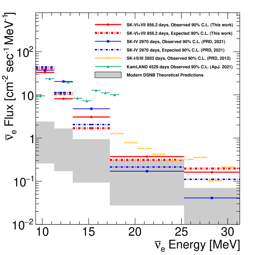
Figure 12: The 90% C.L. upper limits on the astrophysical $\bar{\nu}_{e}$ flux, calculated by Equation 6, per energy bin. The red lines show the observed upper limit (solid, circle point) and expected sensitivity (dot-dashed) for SK-VI+VII. To be conservative, the lines represent the larger values of the two neutron tagging approaches listed in Table 6. The blue lines show the observed upper limit (solid, square point) and expected sensitivity (dot-dashed) for SK-IV Abe et al. (2021). The orange line displays the 90% C.L. observed upper limit for SK-I/II/III without neutron tagging (Bays et al., 2012). The green line with triangle points represents the 90% C.L. observed upper limit placed by KamLAND (Abe et al., 2022b). The gray-shaded regions represent the range of the theoretical flux expectation for the DSNB signal (Malaney, 1997; Hartmann & Woosley, 1997; Kaplinghat et al., 2000; Lunardini, 2009; Horiuchi et al., 2009; Galais et al., 2010; Priya & Lunardini, 2017; Horiuchi et al., 2018; Barranco et al., 2018; de Gouvêa et al., 2020; Kresse et al., 2021; Horiuchi et al., 2021; Tabrizi & Horiuchi, 2021; Ekanger et al., 2022; Ashida et al., 2023; Iváñez-Ballesteros & Volpe, 2023; Nakazato et al., 2024; Martínez-Miravé et al., 2024). The theoretical prediction level is averaged within the bin width.

Table 6: Summary of $\bar{\nu}_{e}$ flux upper limit and sensitivity for each period and neutron tagging algorithm, and optimistic and pessimistic DSNB expectation from Kaplinghat et al. (2000), and Nakazato et al. (2015), respectively. For SK-IV, only BDT-based neutron tagging is applied.

Neutrino Energy	Observed Upper Limit			Expected Sensitivity			DSNB Theoretical Expectation
$\rm[MeV]$	$\rm[cm^{-2}\,s^{-1}\,MeV^{-1}]$			$\rm[cm^{-2}\,s^{-1}\,MeV^{-1}]$			$\rm[cm^{-2}\,s^{-1}\,MeV^{-1}]$
	SK-IV	SK-VI+VII		SK-IV	SK-VI+VII
	BDT	NN	BDT	BDT	NN	BDT
9.29–11.29	37.30	23.79	33.20	34.07	38.26	40.89	0.20 – 2.40
11.29–13.29	20.43	7.48	8.14	11.35	10.32	10.50	0.13 – 1.66
13.29–17.29	4.77	3.07	2.76	2.05	1.67	1.69	0.67 – 0.94
17.29–25.29	0.17	0.37	0.37	0.21	0.31	0.29	0.02 – 0.30
25.29–31.29	0.04	0.13	0.16	0.11	0.20	0.18	$<0.01$ – 0.07

6 DSNB spectral fitting analysis

In the spectral fitting analysis, we extract the normalization of each component (DSNB signal and backgrounds) by fitting their reconstructed PDFs to the data using an extended energy-unbinned likelihood maximization framework. Thus, this analysis leads to a best-fit signal normalization for each DSNB prediction. The main difference here from the spectrum-independent $\bar{\nu}_{e}$ search (Section 5) is that this approach introduces undetermined parameters, namely the absolute event rate of the DSNB signal and backgrounds, as well as certain nuisance parameters for each reconstructed energy PDF shape. In order to further constrain the fit, instead of removing events with background-like $\theta_{c}$ and $N_{\rm n}$, the parameter space is extended to six regions: Three $\theta_{c}$ divisions ($\theta_{c}\in[20^{\circ},\,38^{\circ}]$, $\theta_{c}\in[38^{\circ},\,53^{\circ}]$, $\theta_{c}\in[78^{\circ},\,90^{\circ}]$), and two $N_{\rm n}$ regions ($N_{\rm n}\neq 1$, $N_{\rm n}=1$).

Overall, the principle of the spectral analysis is the same as that detailed in Abe et al. (2021), with three notable differences. First, for the detector, we benefit from enhanced neutron-tagging efficiency due to the Gd-loading in SK-VI and SK-VII, which enhances the DSNB signal detection in the IBD-like region ($\theta_{c}\in[38^{\circ},53^{\circ}]$ and $N_{\rm n}=1$). Next, for the fit, we now profile over all nuisance parameters of the analysis (background rates and shape-only nuisance parameters). Finally, for the data and MC, we update the derivation of the spallation PDF (see Section 6.2 below) and apply the new MSG cut.

6.1 Samples

In this analysis, samples are divided into six regions as described above. The upper bound of the signal energy region is extended to $E_{\rm rec}=79.5$ MeV to take full advantage of the shape and normalization of the signal and backgrounds in the different regions of the parameter space. At the same time, the lower energy threshold of the analysis is set at $E_{\rm rec}=15.5~\rm MeV$ in all regions.

The event selection criteria for the six analysis regions are the same as in the spectrum-independent search from Section 5, with a few exceptions: For the $N_{\rm n}\neq 1$ region, solar neutrinos are removed based on the reconstructed direction of prompt events with the same criteria as in Abe et al. (2021). The new MSG cut is applied only to the middle $\theta_{c}$ region such that atmospheric neutrino events remain in the sideband. The $N_{\rm n}\neq 1$ region contains more spallation events than for $N_{\rm n}=1$ due to the lack of a strict neutron tagging requirement. For this reason, tighter spallation likelihood cuts are applied to the $N_{\rm n}\neq 1$ sample. These are determined by first looking at data without atmospheric background reduction and neutron tagging. Spallation cuts are then varied such that the predicted remaining spallation events in [15.5, 19.5] MeV are approximately at the same level as the predicted peak of decay electrons around 50 MeV. The cut criteria are then progressively loosened until 23.5 MeV. The IBD signal efficiencies of these unique cuts for solar and spallation events for $N_{\rm n}\neq 1$ are given in Table 7.

Table 7: IBD signal efficiency of separate cuts for $N_{\rm n}\neq 1$. The solar neutrino reduction is an additional step, while the spallation values can differ from those for $N_{\rm n}=1$.

Reduction	Energy Region [MeV]
	[15.5, 16.5]	[16.5, 17.5]	[17.5, 18.5]	[18.5, 19.5]	[19.5, 23.5]	[23.5, 79.5]
Solar	0.72	0.81	0.87	0.97	1.0	1.0
SK-VI Spallation	0.73	0.73	0.78	0.78	0.86	0.95
SK-VII Spallation	0.40	0.40	0.46	0.46	0.53	0.98

The background events are divided into five categories: one spallation, one NCQE, and three non-NCQE, contrary to the spectrum-independent analysis. The first of the non-NCQE subcategories is from events with a visible muon or pion in the final state ($\mu/\pi$ background), mainly appearing in the $\theta_{c}\in[20^{\circ},38^{\circ}]$ region. The second comes from electrons stemming from the decay of invisible muons and pions (Decay-$e$ background), while the last is from the charged-current interactions of atmospheric electron neutrinos and antineutrinos with no visible muon or pion in the final state ($\nu_{e}$-CC background). These second and third components reconstruct to the $\theta_{c}\in[38^{\circ},53^{\circ}]$ region. Each event category (backgrounds and DSNB signal) is associated with a PDF across the extended parameter space of the spectral analysis, whose overall event rate is to be fitted to the data samples.

6.2 Spallation Modeling

Spallation events above $E_{\rm rec}=15.5~\rm MeV$ mainly reconstruct to the $N_{\rm n}\neq 1$ and $\theta_{c}\in[38^{\circ},53^{\circ}]$ region. Some of these become accidental coincidences in the $N_{\rm n}=1$ and $\theta_{c}\in[38^{\circ},53^{\circ}]$ region but are negligible due to the low misidentification rate of neutron tagging. Therefore, to generate the spallation PDF, we focus on three isotopes (⁹C, ⁸B, and ⁸Li shown in Figure 2) that will remain in the $N_{\rm n}\neq 1$ and $\theta_{c}\in[38^{\circ},53^{\circ}]$ region after spallation reduction due to their large endpoint energies and high yields. We then combine the reconstructed energy spectra of each of the three spallation isotopes into one global spallation energy spectrum. As in Abe et al. (2021), the following analytical function is then fit to this spectral sum:

$${\rm PDF_{spall}}(E_{\rm rec})\propto\exp\left(-\frac{(E_{\rm rec}+0.511~{\rm MeV})^{\alpha}}{\beta}\right),$$ (7)

where $\alpha$ and $\beta$ are free parameters. This is the baseline PDF shape before taking into account any energy-dependent effects from event selection steps.

To proceed, we should incorporate the impact of applying an energy-dependent cut for reducing solar neutrino events, assuming the same efficiencies as IBD events, summarized in Table 7. These efficiencies rescale the baseline spallation PDF per energy bin. Next, we consider any energy-dependent effects from spallation cuts applied to the spallation PDF. In SK-IV, it was determined that there was no energy dependence on the spallation remaining rate due to the cuts chosen. In contrast, in this analysis, we choose different spallation cut criteria for each energy bin, which induces an energy-dependent impact on the spallation remaining rates. The spallation PDF is therefore reshaped by these rates in each energy bin to obtain the final PDF shape. At these energies, we estimate that our reduction steps after the spallation reduction, i.e., atmospheric neutrino reduction and neutron tagging, have a negligible impact on the spectral shape of the remaining spallation events.

6.3 Systematic Uncertainties

The background-related systematic uncertainties encode the uncertainties in the overall shape of the background PDFs across the entire parameter space $\theta_{c}\otimes\ N_{\rm n}\otimes\ E_{\rm rec}$, while the uncertainty on the integrated signal efficiency is the only signal-related systematic uncertainty considered for the fit. In particular, the uncertainty on the energy scale is assumed to be negligible in this analysis, as it has an insignificant effect on the shape of the PDFs and a negligible impact on the fit results due to the large statistical uncertainties from the small size of our final data samples.

The systematic uncertainty estimates for backgrounds in this analysis remain unchanged from those in  Abe et al. (2021). There are four nuisance parameters to be fitted: $\eta_{\rm spall}$ for the uncertainty in the shape of the spallation PDF, $\eta_{\nu_{e}\rm CC}$ for the uncertainty on the predicted energy-dependent ascending slope of the $\nu_{e}\rm\ CC$ PDF, $\eta_{\rm NCQE}$ for the relative contribution of NCQE events in three $\theta_{c}$ regions, and $\eta_{\rm n}$ for the relative contribution of all event categories between two neutron-tagging regions. To these, we add the one nuisance parameter related to the signal efficiency $\eta_{s}$.

As the background PDFs are area-normalized to one and should be positive across the energy range, these parameters have physical limits. Taking these constraints into account, we assign each parameter a reduced and centered prior distribution, namely a normal distribution for $\eta_{s}$ and $\eta_{\rm spall}$, a folded normal distribution for $\eta_{\nu_{e}\rm CC}$ and $\eta_{\rm n}$, and a log-normal distribution for $\eta_{\rm NCQE}$ (for details, see Appendix F).

6.4 Extended Likelihood

We denote $\vec{\eta}_{b}$ as the 4-vector of the background-related systematics nuisance parameters ($\eta_{\rm spall}$, $\eta_{\rm NCQE}$, $\eta_{\nu_{e}\rm CC}$, $\eta_{\rm n}$), $\vec{N}_{b}$ as the 5-vector of background event rates ($N_{\rm spall}$, $N_{\rm NCQE}$, $N_{\rm{Decay}\ e^{-}}$, $N_{\nu_{e}\rm CC}$, $N_{\mu/\pi}$), and $N_{s}$ as the number of DSNB events corrected from the signal efficiency $\varepsilon_{s}(\eta_{s})$, equal to the number of DSNB events with an energy $E_{\nu}>17.3$ MeV that have occurred in the SK fiducial volume. We note that $\varepsilon_{s}$ differs from $\bar{\epsilon}_{\rm IBD}$ used in Equation 6 of the spectrum-independent search of Section 5 in two aspects: $\varepsilon_{s}$ does not contain the neutron tagging efficiency, given all $N_{\rm n}$ outcomes are included in the two neutron-tagging regions of the spectral analysis; and $\varepsilon_{s}$ is the integrated efficiency over the entire energy range of the spectral analysis and is therefore dependent on the shape of the DSNB model considered. The extended likelihood (Barlow, 1990) to be maximized per phase reads:

$$\mathcal{L}\left(\mathrm{Data}\,\big|\,N_{s},\,\vec{N}_{b},\,\right. \eta_{s} ,\,\vec{\eta}_{b}\Big)=\mathcal{L}\left(\vec{0}\,|\,\eta_{s},\,\vec{\eta}_{b}\right)\,$$

$$\times e^{-\left(\varepsilon_{s}(\eta_{s})N_{s}\ +\ \sum_{j\in\vec{b}}N_{j}\right)}$$

$$\times \prod_{i=1}^{N_{\mathrm{data}}}\Bigl[\varepsilon_{s}(\eta_{s})N_{s}\cdot\mathrm{PDF}_{s}\left(E^{i},\,\theta_{C}^{i},\,N_{\mathrm{n}}^{i}\right)$$

$$\ \ +\sum_{j\in\vec{b}}N_{j}\cdot\mathrm{PDF}_{j}\left(E^{i},\,\theta_{C}^{i},\,N_{\mathrm{n}}^{i}\,|\,\vec{\eta}_{b}\right)\Bigr],$$

where $\mathcal{L}\left(\vec{0}\,|\,\eta_{s},\,\vec{\eta}_{b}\right)$ is the penalty term coming from the product of prior distributions for the nuisance parameters, which have prior values considered to be 0. $\mathrm{PDF}_{s}\left(E^{i},\,\theta_{C}^{i},\,N_{\mathrm{n}}^{i}\right)$ is the signal-related PDF, and $\mathrm{PDF}_{j}\left(E^{i},\,\theta_{C}^{i},\,N_{\mathrm{n}}^{i}\,|\,\vec{\eta_{b}}\right)$ are the background-related PDFs, whose shape may vary depending on the value of the nuisance parameters $\vec{\eta_{b}}$. The exponential term and the $N_{s,\,j}$ parameters account for the Poissonian fluctuations of the rate for each category of event.

To derive the best-fit DSNB event rate across all SK-Gd data, we maximize the sum of the SK-VI and SK-VII log-likelihoods along the common signal efficiency-corrected $N_{s}$ parameter, which is thereafter converted to a DSNB flux value. Confidence intervals for this parameter are then constructed by profiling the likelihood ratio (see Appendix F).

6.5 Results

Using the model from Horiuchi et al. (2009) as a representative prediction of DSNB signal shape, we show in Figure 13 the best-fit results for SK-VI and SK-VII using the NN neutron-tagging algorithm. The best-fit flux range of $2.9^{+2.6}_{-2.0}$ and $0.1^{+1.7}_{-0.1}~\rm cm^{-2}\,s^{-1}$ for SK-VI and SK-VII includes the predicted value of $1.9~\rm cm^{-2}\,s^{-1}$. The best-fit results for SK-VI and -VII using the BDT neutron-tagging algorithm are reported in Appendix F. Additionally, Figure 14 displays the associated phase-combined profile likelihood ratio functions. We can see that samples built using the NN or BDT neutron-tagging algorithm yield statistically compatible results.

The combined fit of SK-Gd data shown as a black line demonstrates a best-fit flux of $1.4^{+1.5}_{-1.2}$ ($1.2^{+1.7}_{-1.2})~\rm cm^{-2}\,s^{-1}$ for the NN (BDT) sample, and rejects the background-only hypothesis at the 1.2$\sigma$ (0.9$\sigma$) level for the case using NN (BDT) neutron tagging, a similar rejection level to the 1.5$\sigma$ result obtained using 5823 days of pure-water SK data (Abe et al., 2021).

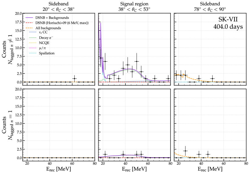
Figure 13: Best-fit results for SK-VI and SK-VII data samples, built out of the NN neutron-tagging algorithm. The input DSNB model used for the fit is Horiuchi et al. (2009).

Repeating the fitting procedure for different DSNB models (Totani & Sato, 1995; Hartmann & Woosley, 1997; Malaney, 1997; Kaplinghat et al., 2000; Ando, 2005; Fukugita & Kawasaki, 2003; Horiuchi et al., 2009; Lunardini, 2009; Galais et al., 2010; Nakazato et al., 2015; Priya & Lunardini, 2017; Barranco et al., 2018; Horiuchi et al., 2018; de Gouvêa et al., 2020; Horiuchi et al., 2021; Kresse et al., 2021; Tabrizi & Horiuchi, 2021; Ashida et al., 2023; Iváñez-Ballesteros & Volpe, 2023; Martínez-Miravé et al., 2024; Nakazato et al., 2024) yields similar confidence intervals, with an excess of $0.7-1.7\sigma$ with the NN-based approach and $0.5-1.3\sigma$ with the BDT-based approach. Frequentist upper limits on the DSNB flux at the 90% C.L. are also derived as follows, in the frame of the Wald asymptotic approximation (Cowan et al., 2011):

$$\mu_{\rm upper,\,90\%\,C.L.}=\hat{\mu}+\sigma\cdot\mathcal{N}^{-1}(90\%),$$ (9)

where $\hat{\mu}$ is the best-fit DSNB flux, $\sigma$ is conservatively estimated as the upper uncertainty on the best-fit value, and $\mathcal{N}$ is the normal cumulative density function. We summarize the spectral fitting results (best-fit flux with $1\sigma$ fitting uncertainty, 90% C.L. upper limit, and significance of excess over backgrounds) for these models in Tables 10 and 11 in Appendix F, and display some in Figure 15. Based on insufficient significance, we conclude that no excess beyond the background-only hypothesis is observed in the spectral analysis of the SK-Gd data.

Yet, we should emphasize that the combined fit results in approximately $\sim 1.4\ \rm{cm}^{-2}~\rm{s}^{-1}$ uncertainty for the DSNB flux, for the Horiuchi+09 model. Noticeably, this is a considerable improvement with respect to the previous pure-water phases. Indeed, with only twice the size of the present SK-Gd dataset, the uncertainty should then become comparable to that of the $\sim$ 6000 days of the SK pure-water phases ($\sim 0.9\ \rm{cm}^{-2}\rm{s}^{-1}$), showing the enhanced sensitivity achieved in the Gd phase.

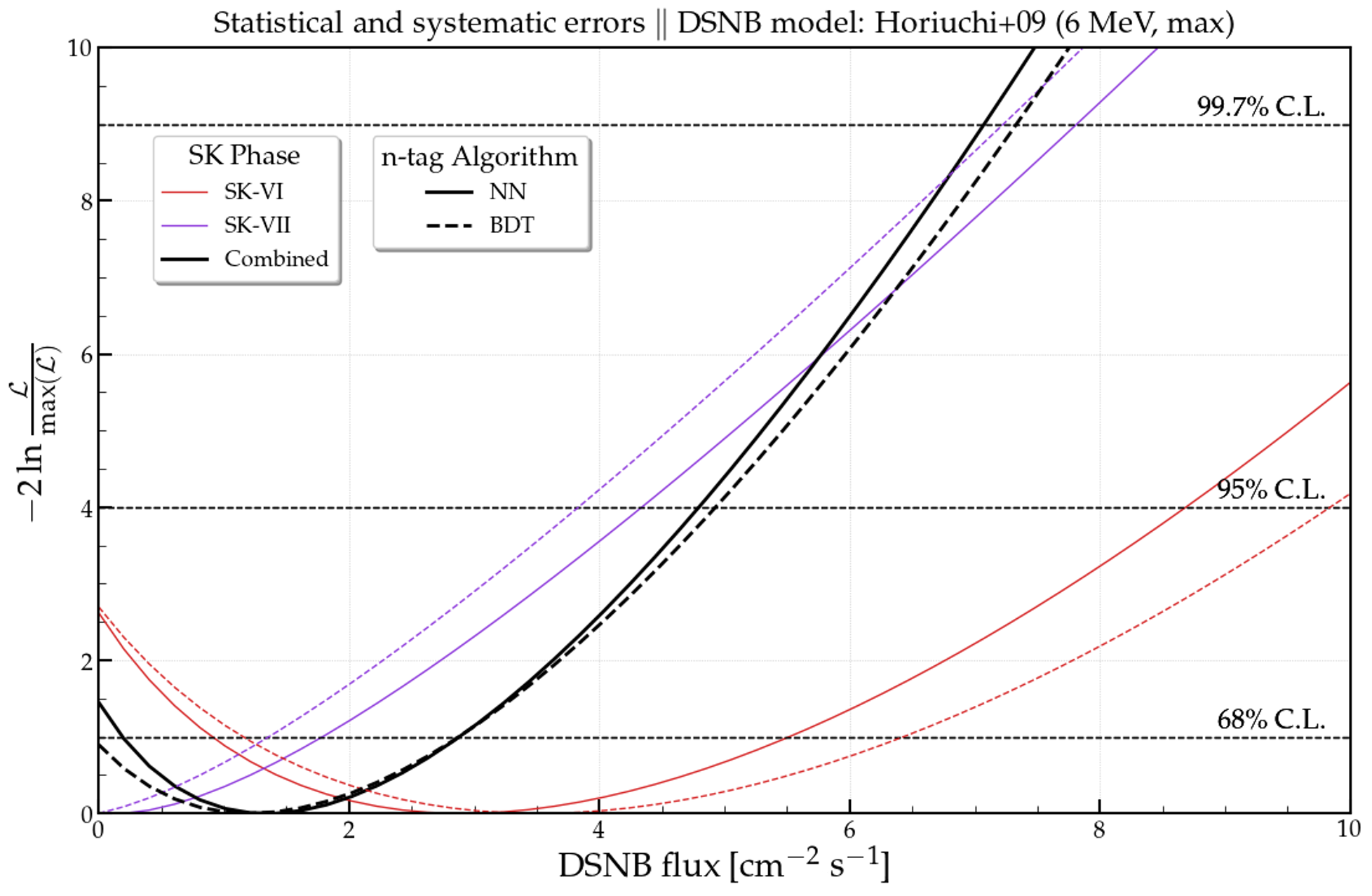
Figure 14: (Logarithm of) profile likelihood ratio as a function of the DSNB flux (for $E_{\nu}>17.3$MeV), for both neutron-tagging algorithms and the DSNB model of Horiuchi et al. (2009). The dotted line shows the significance corresponding to the confidence interval.

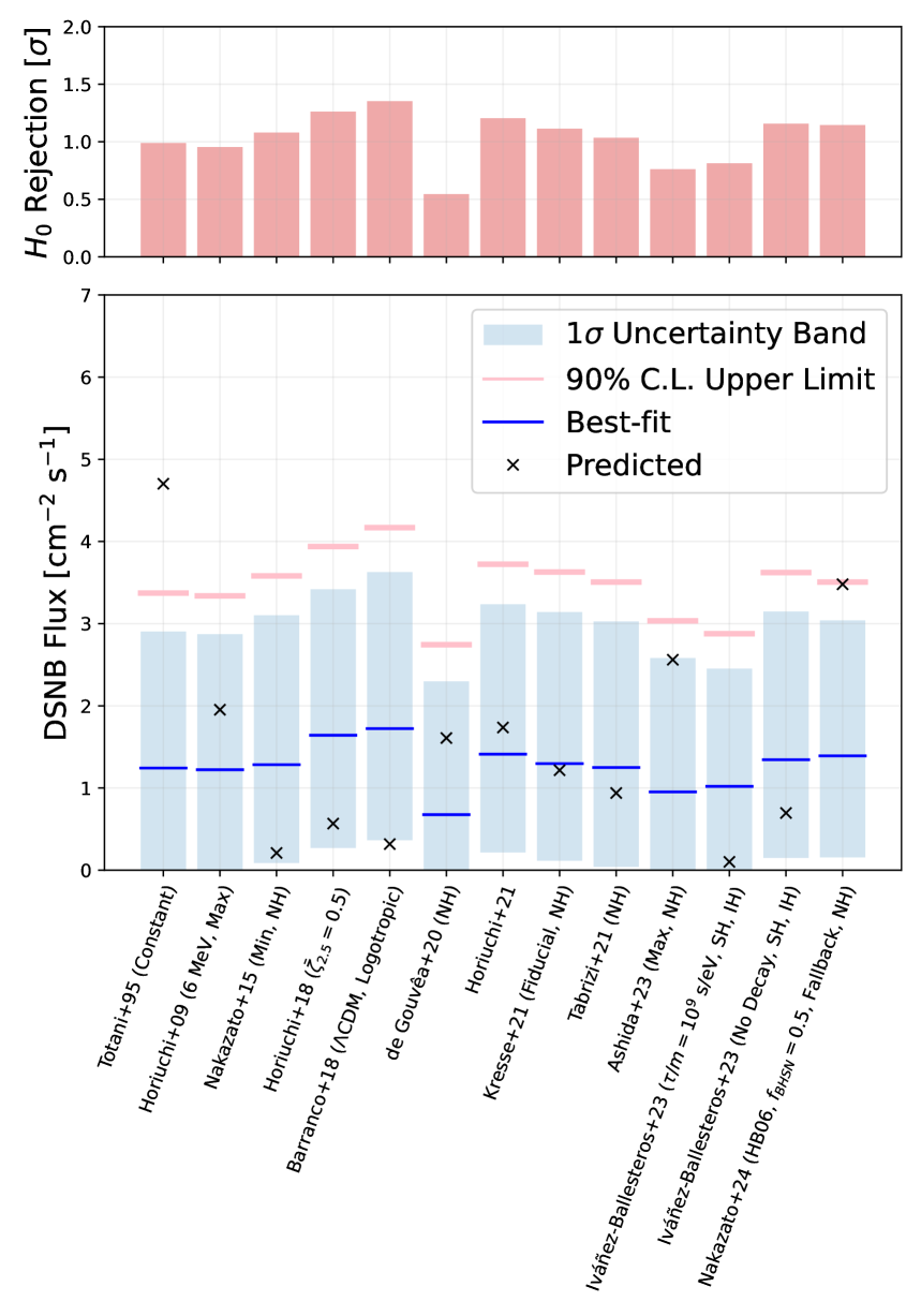
Figure 15: Model-dependent spectral analysis results for DSNB events with $E_{\nu}>17.3$ MeV, obtained with (left) NN and (right) BDT neutron-tagging algorithms. (bottom) $1\sigma$ uncertainty bands and 90% C.L. upper limits on the DSNB flux, as well as (top) rejection of the background-only hypothesis $H_{0}$ for a variety of input DSNB model shapes (Totani & Sato, 1995; Hartmann & Woosley, 1997; Malaney, 1997; Kaplinghat et al., 2000; Ando, 2005; Fukugita & Kawasaki, 2003; Horiuchi et al., 2009; Lunardini, 2009; Galais et al., 2010; Nakazato et al., 2015; Priya & Lunardini, 2017; Barranco et al., 2018; Horiuchi et al., 2018; de Gouvêa et al., 2020; Horiuchi et al., 2021; Kresse et al., 2021; Tabrizi & Horiuchi, 2021; Ashida et al., 2023; Iváñez-Ballesteros & Volpe, 2023; Martínez-Miravé et al., 2024; Nakazato et al., 2024). For the sake of completeness, results with additional DSNB model shapes from (Kresse et al., 2021; Iváñez-Ballesteros & Volpe, 2023; Martínez-Miravé et al., 2024; Nakazato et al., 2024) are shown in Appendix F. “NH” and “IH” refer to the normal and inverse neutrino mass hierarchies, respectively. “MD14” corresponds to the SFR calculations performed by Madau & Dickinson (2014). For the models from Iváñez-Ballesteros & Volpe (2023), “SH” stands for “strongly hierarchical”. Finally, “CE”, “CGI” and “HMA” stand for “chemical evolution”, “cosmic gas infall” and “heavy metal abundance” respectively for models Hartmann & Woosley (1997), Malaney (1997) and Kaplinghat et al. (2000). For more information on the models, please refer to the various publications.

7 Discussion

The spectral-fitting results indicate an excess over the background-only hypothesis at the $\sim$ $1\sigma$ level for many DSNB models. Despite the large variation of flux shapes from different modeling approaches, the best-fit values and $1\sigma$ intervals do not differ significantly. This suggests that changes in model parameters may not be distinguishable given the current statistical and systematic uncertainties. However, in some steeply decreasing flux models with extremely low event rates, such as certain parameter sets of Iváñez-Ballesteros & Volpe (2023), de Gouvêa et al. (2020), and Barranco et al. (2018), our fitting is already sensitive to their particular shape, which causes the best-fit DSNB flux and $1\sigma$ intervals to differ from the majority of models. For example, the best-fit value of the minimum flux case of the Nakazato et al. (2015) model is comparable to other best-fit values, yet it is slightly above the theoretically predicted value. This suggests that the true flux level might be higher than conservative estimates indicate. In contrast, models with a large black-hole-formation effect, such as Nakazato et al. (2024) with $f_{\rm BHSN}=0.5$, the maximum case of Kaplinghat et al. (2000), and the maximum case of Ashida et al. (2023), possibly overestimate their parameter assumption: These predicted flux values are above their $1\sigma$ best-fit ranges. Finally, as another illustration, Iváñez-Ballesteros & Volpe (2023) implements different neutrino decay scenarios which, depending on their lifetime and mass hierarchy, can modify the electron antineutrino flux to a greater or lesser extent.

Given the importance of neutron identification for the SK DSNB search, we employed two machine learning techniques — the newly developed NN and the updated BDT. Since they are constructed, trained, and tuned independently, this adds robustness to the results; indeed, the NN and BDT arrive at similar performance levels for distinct reasons. Moreover, the physics inferred from our data is consistent across neutron identification techniques for both statistical analysis approaches.

Enabled by the new MSG reduction targeting NCQE and other multi-cone events, we have demonstrated how these backgrounds become subdominant after cut optimization, as illustrated across all bins in Figure 11. In the spectral fit example of Figure 13, we observe that a negligible amount of NCQE is fitted in the signal-rich $\theta_{c}$ region. While this NCQE reduction comes at a further cost to the IBD signal efficiency, the background removal is highly effective. Further improvements may be achieved through machine learning approaches, such as that proposed by Maksimović et al. (2021).

Moving forward, there remain two dominant backgrounds in the SK-Gd DSNB search. The first are the decays of invisible muons and pions at higher energies. The second, in contrast, are spallation products that dominate at the lowest energies. The current data-driven method for extracting spallation event characteristics heavily relies on statistics. In addition, evaluating the ability to remove spallation events relies on physics assumptions, which cause significant uncertainty above 50% for the ${}^{9}\rm Li$ remaining rate. A better understanding of cosmic-ray muon interactions in water and the development of a reliable spallation simulation are crucial for improving background reduction, more accurate spallation event PDFs, and a reasonable estimation of the isotope remaining rate. This will lead to more strict constraints on the DSNB flux in the region where the flux is largest.

In this study, we presented a reliable data-driven method for estimating the non-NCQE normalization uncertainty. However, further suppressing this uncertainty is limited by the statistics of the sideband samples. The DSNB flux prediction in the higher energy region is largely affected by black hole formation: The longer accretion phase makes the neutron star hotter, such that the energy of emitted neutrinos is higher. In the future, searches with larger SK-Gd datasets will enable access to the black-hole-formation history (Ashida & Nakazato, 2022; Ashida et al., 2023), made possible by increased statistics in the sideband region. Additionally, new nuclear interaction models, once validated by the data from neutrino experiments, have the potential to reduce the uncertainties in the atmospheric neutrino background. Notably, better modeling of the neutron multiplicity in atmospheric neutrino interactions will be crucial for the discovery of DSNB, since we employ neutron tagging to enhance sensitivity.

8 Conclusion

We have analyzed 956.2 livedays of SK-Gd data with two parallel statistical approaches for the DSNB search. Given the importance of prompt and delayed signal coincidence, we used two machine learning algorithms to identify neutron captures for the first time in SK-Gd. In addition, we implemented a new background reduction technique targeting atmospheric neutrino interactions. In a DSNB spectrum-independent search, we searched for the DSNB signal in the 7.5 to 29.5 MeV energy range, and observed no significant excess over background predictions. Then, we set new upper limits on the astrophysical $\bar{\nu}_{e}$ flux. In this time, we updated the world’s most stringent limits in the energy region 9.29-11.29 MeV to $33.2~\rm cm^{-2}\,s^{-1}\,MeV^{-1}$, in the energy region 11.29–13.29 MeV to $8.14~\rm cm^{-2}\,s^{-1}\,MeV^{-1}$, and 13.29-17.29 MeV to $2.76~\rm cm^{-2}\,s^{-1}\,MeV^{-1}$. In a DSNB spectral fit, we observed an approximately 1.2$\sigma$ (0.9$\sigma$) rejection of a background-only hypothesis for the majority of DSNB models considered while using an NN-based (BDT-based) neutron capture identification algorithm.

Appendix A Neutron cloud cut with Gd

Regarding the neutron cloud cut, the neutron detection method follows Shinoki et al. (2023) completely. To remove neutron-correlated spallation events, we use the timing difference of muons ($\Delta t$) and spatial correlation ($\Delta L^{\rm cloud}$) of the barycenter of reconstructed neutron cloud vertices from DSNB candidates to reduce spallation events close to the hadronic shower. In addition, a more sophisticated elliptical shape cut along with the reconstructed muon track is applied, using transverse distance from muon track($\ell_{t}$) and the position difference between neutron cloud and DSNB candidate along with the muon track ($L^{\rm cloud}_{l}$). We utilize the same muon reconstruction algorithm as one used in Kitagawa et al. (2024), detailed in Conner (1997) and Desai (2004). The definitions of $\Delta L^{\rm cloud}$, $L^{\rm cloud}_{l}$, and $\ell_{t}$ are illustrated in Figure 16.

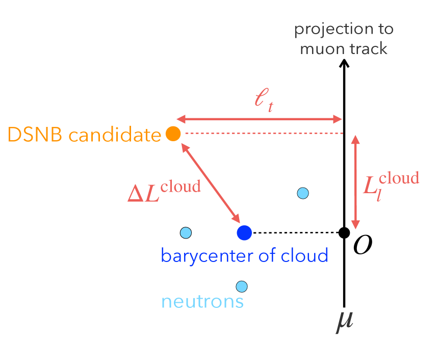
Figure 16: Illustration of neutron cloud variables.

Conservatively, we apply the same cut threshold as in the SK-IV analysis (Locke et al., 2024) since the timing difference between muon and spallation product should not have large differences. The vertex resolution improvement due to Gd has a minimal impact on the neutron cloud vertex.

To extract the neutron cloud cut performance, at first, we separate muon samples within $\pm 60~\rm s$ around DSNB candidates into pre-sample and post-sample, which are the prior and posterior timing muons, respectively, as illustrated in Figure 17. The muon responsible for causing spallation is included only in the pre-sample, and all other muons in the pre-sample and all post-sample muons should not be correlated with the DSNB candidates. This concept is used for the likelihood approach, as described below.

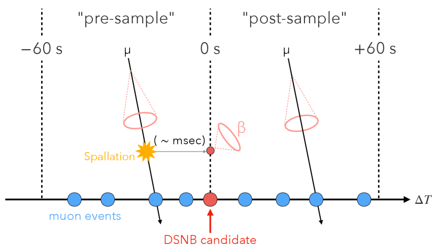
Figure 17: Illustration of the separation for pre- and post-sample regions.

Figure 18 shows an example of the $\Delta L^{\rm cloud}$ for pre- and post-sample muons. A clear correlation is found in small $\Delta L^{\rm cloud}$ only in the pre-sample, and good consistency is seen in large distances exceeding 10 m.

Figure 18: $\Delta l$ distribution between a DSNB candidate and the muon events before and after the candidate.

The efficiency of the neutron cloud cut for both signal and background is calculated using pre- and post-sample data, following the same method as in previous works (Abe et al., 2021). As a result, this cut removes 51% of spallation events while keeping 98% of the signal.

Appendix B MSG cut to NCQE event reduction

Figure 19 shows the reduction efficiency of NCQE events. The Cherenkov angle cut and the MSG cut are the most effective in reducing NCQE events. In higher energy regions, many NCQE events have multiple Cherenkov cones and can easily be reduced by the Cherenkov angle cut due to their topology. On the other hand, the lower energy events have a single-cone-like pattern or do not generate enough PMT hits to be identified as multiple cones, resulting in a worse reduction efficiency. The MSG cut is effective for these lower-energy events and complements the Cherenkov angle cut. This is because MSG exploits the finer structure of the PMT hit topology (again, originally to quantify the multiple scattering of electrons). Overall, the effect of MSG cut on NCQE is the strongest in regions for which NCQE events dominate the DSNB signal compared to other backgrounds, which is roughly in the energy range of $E_{\rm rec}\in$ [9.5, 19.5] MeV. The energy-dependent MSG threshold values in the analysis are given in Table 8.

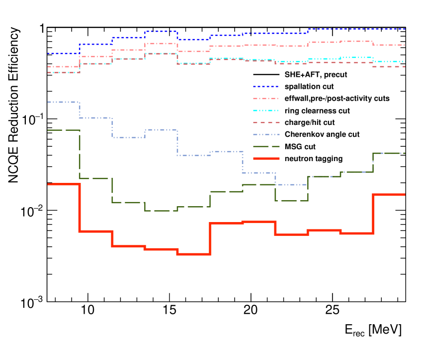
Figure 19: NCQE event reduction efficiency for each cut step in SK-VI. These lines show accumulated efficiencies at each stage.

Table 8: MSG event selection threshold values as a function of energy $E_{\rm rec}$.

Energy [MeV]	MSG Threshold Value
$[7.5,~9.5]$	0.39
$[9.5,~11.5]$	0.43
$[11.5,~13.5]$	0.47
$[13.5,~15.5]$	0.42
$[15.5,~17.5]$	0.37
$[17.5,~19.5]$	0.36
$[19.5,~21.5]$	0.35
$[21.5,~23.5]$	0.32

Appendix C NN Neutron Tagging

The NN neutron tagging tool searches for peaks using a 14 ns sliding window with a 7-hit threshold to the time-of-flight corrected PMT-hit timing distribution. For each cluster, we calculate feature variables; two types of the number of hits, such as 14 ns window ($N_{\rm hits}$) and $\pm$ 100 ns window ($N_{200}$), root-mean-square (RMS) of PMT hits from timing peak ($T_{\rm RMS}$), spherical harmonics parameters used in Bellerive et al. (2016) ($\beta_{1}$ and $\beta_{5}$), mean and RMS from the angle between each hit and averaged hit direction ($\theta_{\rm dir}^{\rm mean}$ and $\theta_{\rm dir}^{\rm RMS}$), mean, RMS, and skewness of the opening angle formed by three-hit combinations ($\theta_{\rm angle}^{\rm mean}$, $\theta_{\rm angle}^{\rm RMS}$, and $\theta_{\rm angle}^{\rm Skew}$), and the two kinds of distance of the prompt event from the ID wall ($d_{\rm wall}$) and $d_{\rm eff}$.

For the classification algorithm, we adopt a feed-forward Multilayer-Perceptron (MLP) implemented using the TMVA library (Therhaag, 2010) as the NN algorithm. This NN is trained using $7\times 10^{5}$ events of IBD MC with an architecture of 0.02 as the learning rate, 14:15:13:1 as the layers, and using the sigmoid function for neuron activation.

To determine the selection criteria for the NN output score, we first explored the working neutron search window, which was 535 $\mu$s in SK-IV, because the increasing cross section of neutron captures in SK-Gd makes the neutron capture timing shorter. We applied an NN neutron selection to the signal MC with various combinations of NN score criteria and capture time criteria, ensuring $f_{\rm mis}$ remains about $\mathcal{O}(10^{-4})$ level. We optimized the time window to obtain the highest signal efficiency, as shown by the orange marker in Figure 9. As a result, we successfully reduced the search time window range to $270~\mu$s and lowered the NN score threshold in SK-VII. The optimal criteria for the NN score are determined to be 0.99 for SK-VI and 0.98 for SK-VII.

Appendix D BDT Neutron Tagging

The BDT neutron search algorithm makes use of PMT hit clusters passing a pre-selection condition of at least 6 hits in a time-of-flight subtracted timing sliding window of 10 ns ($N_{10}$) starting 2 $\mu$s (in SK-Gd) after the prompt peak, going until 535 $\mu$s. This TOF is defined using the reconstructed prompt vertex with the understanding that IBD neutrons at these energies will not be captured far from the prompt vertex. After this, an attempt is made at reconstructing the neutron capture vertex to build other relevant observables. The BDT was trained on IBD MC, such that the relationship between the neutron capture vertex and the prompt vertex can be exploited with realistic neutron energies. Of the 22 total input variables, there are 9 (including $N_{10}$) that focus on the neutron capture vertex, another 7 focused on the Cherenkov light specifically, and a final 6 targeting noise hits. After $N_{10}$, the 5 most important input variables in SK-Gd (quantified by BDT F-score) are the number of PMT hits in clusters of at least 3 within 14.1^∘ ($N_{c}$), the number of PMT hits with a low probability of originating from the reconstructed neutron capture vertex ($N_{\text{low}}$), the mean opening angle of the PMT hits ($\theta_{m}$), the distance of the neutron capture vertex from the detector walls (f${}_{\text{wall}}$), and the distance between the reconstructed prompt vertex and neutron capture vertex (fp${}_{\text{dist}}$). A list of all BDT input variables and their definitions is shown in Table 9.

For this study, it was important to ensure a low misidentification rate where no-neutron spallation dominates for $E_{\rm rec}<29.5$ MeV. To this end, we added a pre-selection step for samples for BDT Neutron tagging, using $N_{10}$, $N_{c}$, and the number of reconstructed Cherenkov photons from the delayed vertex (bse) per $N_{10}$ window. Misidentification is more likely when there are low hits for $N_{10}$, few hits in clusters with $N_{c}$, and few Cherenkov photons reconstructed for bse. We reject neutron candidates for which $N_{10}<13$ and $N_{c}=0$, as well as those for which $N_{10}<13$ and bse $<20$. For SK-VII, this results in a misidentification rate of around 0.05% at 64% signal efficiency, which is about half the misidentification rate of the BDT’s nominal performance at this signal efficiency. This pre-selection is taken into account for the performance shown in Figure 9.

Table 9: BDT input variable names and definitions.

Variable	Definition
$N_{10}$	Number of PMT hits in a 10 ns TOF-corrected window from reconstructed prompt vertex.
$\Delta N_{10}$	Change in $N_{10}$ after using TOF correction from reconstructed delayed vertex instead.
$t_{\rm RMS}$	RMS of PMT hit times.
$\Delta t_{\rm RMS}$	Change in $t_{\rm RMS}$ after using TOF correction from reconstructed delayed vertex instead.
$\rm fp_{dist}$	Distance between reconstructed prompt vertex and delayed vertex.
$\rm bp_{dist}$	Difference between delayed vertex reconstructed position from two different approaches.
bse	Reconstructed number of emitted Cherenkov photons emitted from the delayed vertex.
$\rm f_{wall}$	Distance of reconstructed delayed vertex (from minimizing TOF residuals within 2 m of prompt vertex) from detector wall.
$\rm b_{wall}$	Distance of BONSAI-reconstructed delayed vertex from detector wall.
$\theta_{\rm mean}$	Mean PMT hit opening angle calculated from the average PMT hit direction from the prompt vertex.
$\theta_{\rm RMS}$	RMS of the PMT hit opening angles.
$\phi_{\rm RMS}$	RMS of azimuthal separation between PMT hits.
$N_{\rm back}$	Number of PMT hits in the backward hemisphere from the average PMT hit direction.
$N_{\rm low\theta}$	Number of hits within opening angle of $20^{\circ}$.
$N_{\rm clus}$	Number of PMT hits inside a cluster of 3 separated by $14.1^{\circ}$.
$N_{\rm low}$	Number of PMT hits who are unlikely given the TOF information from the reconstructed delayed vertex.
$Q_{\rm mean}$	Mean charge deposited per PMT hit.
$Q_{\rm RMS}$	RMS of PMT hit charge deposited.
$N_{\rm highQ}$	Number of PMT hits with high charge deposited.
$N_{300}$	Number of PMT hits in 300 ns window around original $N_{10}$ window.
$t_{\rm RMS}^{(3)}$	Minimum RMS of hit times in subset of 3 hits.
$t_{\rm RMS}^{(6)}$	Minimum RMS of hit times in subset of 6 hits.

Appendix E Comparison of Americium-Beryllium calibration

As mentioned in Section 4.5, we validate our neutron detection techniques using an Am/Be neutron source. The measurement configuration is detailed in Harada (2022). We took data at nine source points in the SK tank equally $-12$, $0$, and $12~\rm m$ for the $x$ and $z$-axes, and monthly at the center point. Then, we evaluated the position dependence and time variation of neutron detection performance. The main purpose of this measurement is to check the consistency between the data and the MC sample for our neutron detection technique. Figure 20 shows the distribution of the NN score of neutron candidates in the Am/Be measurement. The MC contains the true neutron capture events on Gd, protons, and noise candidates. The overall shape shows good agreement between the data and the MC samples. We evaluated the neutron detection efficiency for both the data and MC samples, as well as their ratio as a function of the NN score. The results for SK-VII is shown in Figure 21. There are discrepancies between the data and the MC sample around the NN working point, with 8.4% and 3.4%, in SK-VI and SK-VII, respectively. The position dependence and time variation of the neutron detection efficiency are negligibly small and stable compared to the size of the discrepancy. Thus, we assigned this difference to the systematic uncertainty of neutron detection. We also use this Am/Be data to estimate the systematic uncertainty associated with BDT neutron detection. Following the same procedure of comparing data to MC for detection efficiency, we find a maximum discrepancy for the BDT of 5% and 6% for SK-VI and SK-VII, respectively. Figure 22 shows the BDT comparison for one Am/Be run in SK-VII as an example.

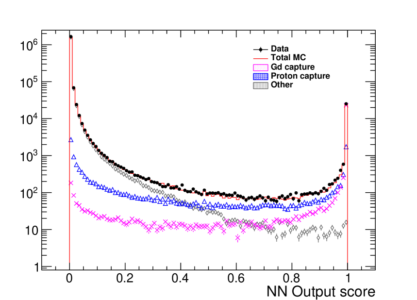
Figure 20: NN score distribution of Am/Be data sample and MC in SK-VII. The red line shows the accumulated histogram among the Gd (Magenta cross) and proton (Blue triangle), and noise (Gray diamond). Each plot is normalized by the number of prompt events.

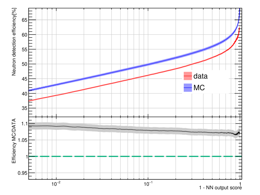
Figure 21: Neutron detection efficiency evaluated by Am/Be data and MC sample using NN algorithm (top) and its ratio between data/MC, as a function of cut criteria of NN score in SK-VI. The error band shown with the data represents statistical uncertainty, and with MC, it means the combination of statistical and systematic uncertainties.

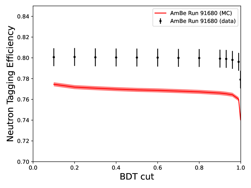
Figure 22: Neutron selection efficiency for BDT as a function of BDT score threshold in one Am/Be run. Statistical error bars are shown on the data with a statistical error band for the MC prediction.

Appendix F Spectral fit details

F.1 Nuisance parameters

We provide the details below about the five nuisance parameters considered in the spectral analysis, as detailed in Beauchêne (2024). All parameters are expressed in units of standard deviation and assigned a centered and reduced probability density function, i.e., whose mean and standard deviation are, respectively, 0 and 1.

F.1.1 Signal efficiency: $\eta_{s}$

The number of DSNB signal events to be fitted in the likelihood of Equation (6.4) is $\varepsilon_{s}(\eta_{s})N_{s}$. More specifically, we have: $\varepsilon_{s}(\eta_{s})=\varepsilon_{s}^{0}\times(1+\sigma_{s}\eta_{s})$, with $\varepsilon_{s}^{0}$ the nominal signal efficiency and $\sigma_{s}$ the total uncertainty on this value. This uncertainty includes the uncertainties related to the event selection criteria, the IBD cross section, and the phase livetime, which are summed in quadrature, amounting to $\sim 3\%$ total uncertainty for both SK-VI and -VII. $\eta_{s}$ is associated with a standard normal probability density function.

F.1.2 Atmospheric $\nu_{e}$ CC interactions: $\eta_{\nu_{e}\rm CC}$

As reported in the SK-I to -IV analysis (Abe et al., 2021), Monte-Carlo simulations predict a linear increase in the reconstructed energy of the spectrum for this event category. A 50% systematic uncertainty on the slope of the spectrum is assigned by the formula to the right of the right arrow, fully correlated between the two neutron-detected regions:

$$\mathrm{PDF} {}_{\nu_{e}\rm CC}(E_{\rm rec})\to\mathrm{PDF}_{\nu_{e}\rm CC}(E_{\rm rec})$$ (F1)

$$\times \left(1+\sigma_{\nu_{e}\rm CC}\,\eta_{\nu_{e}\rm CC}\,\frac{E_{\rm rec}-15.5\ [\mathrm{MeV}]}{79.5-15.5\ [\mathrm{MeV}]}\right)$$

where $15.5$ (resp. $79.5$) MeV is the lower (resp. upper) boundary of the spectral analysis in the reconstructed energy window, and $\sigma_{\nu_{e}\rm CC}=50\%$. Therefore, $\eta_{\nu_{e}\rm CC}$ is bound to be greater than $-2$ and is assigned a folded normal probability density function to preserve this feature.

F.1.3 NCQE interactions: $\eta_{\rm NCQE}$

NCQE-type events exhibit a distinct angular distribution in the large Cherenkov angle region, associated with a significant uncertainty due to the challenging modeling of multiple secondary gammas emitted in these interactions. A significant portion of these events may therefore be misclassified in the signal Cherenkov angle region. Following the approach of Abe et al. (2021), we parameterize this effect as a 100% systematic uncertainty on the number of NCQE events in the signal (medium) Cherenkov angle region, fully correlated between neutron-tagged regions:

$$\begin{array}[]{l}\mathrm{PDF}_{\mathrm{NCQE}}^{\mathrm{High}\,\theta_{c}}\to\mathrm{PDF}_{\mathrm{NCQE}}^{\mathrm{High}\,\theta_{c}}\times(1-\sigma_{\mathrm{NCQE}}\,A^{\mathrm{High}\,\theta_{c}}_{\mathrm{NCQE}}\,\eta_{\mathrm{NCQE}}),\\ \mathrm{PDF}_{\mathrm{NCQE}}^{\mathrm{Medium}\,\theta_{c}}\to\mathrm{PDF}_{\mathrm{NCQE}}^{\mathrm{Medium}\,\theta_{c}}\times(1+\sigma_{\mathrm{NCQE}}\,\eta_{\mathrm{NCQE}}),\\ \mathrm{PDF}_{\mathrm{NCQE}}^{\mathrm{Low}\,\theta_{c}}\to\mathrm{PDF}_{\mathrm{NCQE}}^{\mathrm{Low}\,\theta_{c}}\times(1-\sigma_{\mathrm{NCQE}}\,A^{\mathrm{Low}\,\theta_{c}}_{\mathrm{NCQE}}\,\eta_{\mathrm{NCQE}}),\end{array}$$ (F2)

where $\sigma_{\mathrm{NCQE}}=100\%$, $A^{\mathrm{High}\,\theta_{c}}_{\mathrm{NCQE}}$ and $A^{\mathrm{Low}\,\theta_{c}}_{\mathrm{NCQE}}$ are normalization factors introduced to preserve the overall normalization of the PDF across the six regions. $\eta_{\rm NCQE}$ is bound to be greater than $-1$. To fulfill this condition while maintaining a zero mean and unit standard deviation, this parameter is assigned a log-normal probability density function.

F.1.4 Spallation events: $\eta_{\rm spall}$

Spallation events, mainly those from ⁸B, ⁸Li, and ⁹C isotopes, contribute to the background in the signal region of the spectral analysis. To model the shape uncertainty associated with the spallation spectrum, we follow the procedure in Abe et al. (2021) and introduce a nuisance parameter $\eta_{\rm spall}$, modifying the spallation event PDF as:

$$\mathrm{PDF}_{\rm spall} (E_{\rm rec})$$

$$\rightarrow \mathrm{PDF}_{\rm spall}(E_{\rm rec})\times\left(1+\eta_{\rm spall}\,\mathcal{P}_{3}(E_{\rm rec})\right),$$

where $\mathcal{P}_{3}(E_{\rm rec})$ is a third-order polynomial denoting the energy-dependent 1$\sigma$ uncertainty on the spallation PDF shape, stemming from the uncertainty on the relative contribution of each isotope to the spallation background event rate. $\eta_{\rm spall}$ is assigned a standard normal probability density function.

F.1.5 Neutron tagging: $\eta_{\rm n}$

As in Abe et al. (2021), the uncertainty related to neutron tagging efficiency is dominated by the uncertainty in the neutron multiplicity and found to be approximately $40\%$. The effect is parametrized by a dedicated nuisance parameter as follows:

$$\begin{array}[]{rl}\mathrm{PDF}_{j}^{N_{\mathrm{n}}=1}&\to\mathrm{PDF}_{j}^{N_{\mathrm{n}}=1}\times(1+\sigma_{N_{\mathrm{n}}}\,\eta_{N_{\mathrm{n}}}),\\ \mathrm{PDF}_{j}^{N_{\mathrm{n}}\neq 1}&\to\mathrm{PDF}_{j}^{N_{\mathrm{n}}\neq 1}\times(1-\sigma_{N_{\mathrm{n}}}\,A_{N_{\mathrm{n}}}\,\eta_{N_{\mathrm{n}}}),\end{array}$$ (F4)

where $\sigma_{N_{\mathrm{n}}}=40\%$, and $A_{N_{\mathrm{n}}}$ is a relative normalization parameter. $\eta_{\rm n}$ is therefore bound to be greater than $-2.5$ and is assigned a folded normal probability density function.

We show in Figure 23 the probability density functions associated with the aforementioned nuisance parameters $\mathcal{L}(0\,|\,\eta)$. The overall penalty term in Equation (6.4) reads $\mathcal{L}\left(\vec{0}\,|\,\vec{\eta}\right)=\prod_{\eta}\mathcal{L}(0\,|\,\eta)$.

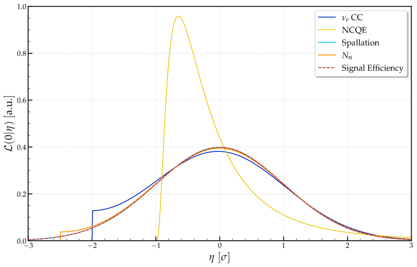
Figure 23: Prior probability density functions for the nuisance parameters of the spectral analysis.

F.2 Likelihood ratio

In the fit of the spectral analysis, the chosen statistical approach is to profile the likelihood ratio over all the nuisance parameters of the analysis, namely the background rates $\vec{N}_{b}$, the PDFs shape-only nuisance parameters and signal efficiency nuisance parameter $\vec{\eta}_{b},\,\eta_{s}:=\vec{\eta}$. This means that the likelihood ratio function $\mathcal{L_{R}}$, whose logarithm is displayed in Figure 14, is obtained as follows:

$$\mathcal{L_{R}}(N_{s})=\frac{\mathcal{L}\left(\mathrm{Data}\,|\,N_{s},\,\hat{\hat{\vec{N}}}_{b},\,\hat{\hat{\vec{\eta}}}\right)}{\mathcal{L}\left(\mathrm{Data}\,|\,\hat{N_{s}},\,\hat{\vec{N}}_{b},\,\hat{\vec{\eta}}\right)},$$ (F5)

where $\mathcal{L}\left(\mathrm{Data}\,|\,\hat{N_{s}},\,\hat{\vec{N}}_{b},\,\hat{\vec{\eta}}\right)$ is the likelihood maximized over the entire parameter space $\{N_{s},\,\vec{N}_{b},\,\vec{\eta}\}$, whereas $\mathcal{L}\left(\mathrm{Data}\,|\,N_{s},\,\hat{\hat{\vec{N}}}_{b},\,\hat{\hat{\vec{\eta}}}\right)$ is the likelihood maximized over the restricted parameter space $\{\vec{N}_{b},\,\vec{\eta}\}$ at fixed $N_{s}$.

This derivation of the likelihood ratio function slightly differs from the one adopted in the SK-I to -IV analysis of Abe et al. (2021), where the profiling was done only over background rate, whereas the PDFs shape-only and signal efficiency nuisance parameters were marginalized, i.e., integrated over in the computation of the likelihoods.

F.3 Other results

In Figure 24, we display the result of the best-fit for the SK-VI and -VII BDT-samples, obtained with the Horiuchi et al. (2009) model as an input DSNB signal shape. Finally, Tables 10 and 11 list the results of the spectral analysis for various DSNB model shapes, including the ones displayed in Figure 15.

Figure 24: Best-fit results for SK-VI and -VII data samples, built out of BDT neutron-tagging algorithm. The input DSNB model used for the fit is Horiuchi et al. (2009).

Table 10: Model-dependent spectral analysis results for DSNB events with $E_{\nu}>17.3$ MeV, obtained with the NN-based neutron-tagging algorithm. “NH” and “IH” refer to the normal and inverted neutrino mass hierarchies, respectively. “HB06” and “MD14” correspond to the SFR calculations performed by Hopkins & Beacom (2006) and Madau & Dickinson (2014) respectively. For the models from Iváñez-Ballesteros & Volpe (2023), “SH” stands for “strongly hierarchical”.

Model	Best-fit $[$cm-2 s${}^{-1}]$	90% Upper Limit $[$cm-2 s${}^{-1}]$	Predicted $[$cm-2 s${}^{-1}]$	$H_{0}$ Rejection $[\sigma]$
Totani+95 (Constant)	$1.4^{+1.5}_{-1.2}$	3.4	4.7	1.2
Hartmann+97 (CE)	$1.5^{+1.6}_{-1.2}$	3.6	0.6	1.3
Malaney+97 (CGI)	$1.6^{+1.7}_{-1.1}$	3.8	0.3	1.4
Kaplinghat+00 (HMA, Max)	$1.5^{+1.7}_{-1.2}$	3.7	3.0	1.4
Kawasaki+03	$1.5^{+1.7}_{-1.2}$	3.6	0.7	1.3
Ando+03 (Updated 05)	$1.5^{+1.6}_{-1.2}$	3.5	0.7	1.3
Horiuchi+09 (6 MeV, Max)	$1.4^{+1.5}_{-1.2}$	3.3	2.0	1.2
Lunardini+09 (Failed SN)	$1.4^{+1.6}_{-1.2}$	3.4	0.7	1.2
Galais+10 (NH)	$1.5^{+1.5}_{-1.2}$	3.4	1.6	1.3
Galais+10 (IH)	$1.5^{+1.5}_{-1.2}$	3.5	1.5	1.3
Nakazato+15 (Min, NH)	$1.5^{+1.6}_{-1.2}$	3.6	0.2	1.3
Nakazato+15 (Max, IH)	$1.4^{+1.4}_{-1.2}$	3.3	0.5	1.2
Priya+17 (NH)	$1.5^{+1.7}_{-1.2}$	3.7	0.4	1.4
Horiuchi+18 ($\bar{\zeta}_{2.5}=0.1$)	$1.4^{+1.4}_{-1.2}$	3.3	1.2	1.2
Horiuchi+18 ($\bar{\zeta}_{2.5}=0.5$)	$1.9^{+1.7}_{-1.3}$	4.1	0.6	1.6
Barranco+18 ($\Lambda$CDM, Logotropic)	$2.0^{+1.9}_{-1.3}$	4.4	0.3	1.7
De Gouvêa+20 (NH)	$0.8^{+1.4}_{-0.8}$	2.6	1.6	0.7
Horiuchi+21	$1.6^{+1.7}_{-1.2}$	3.8	1.7	1.5
Kresse+21 (Fiducial, NH)	$1.5^{+1.7}_{-1.2}$	3.7	1.2	1.4
Kresse+21 (Fiducial, IH)	$1.5^{+1.7}_{-1.2}$	3.6	1.0	1.4
Kresse+21 (Low, NH)	$1.5^{+1.7}_{-1.2}$	3.7	1.0	1.4
Kresse+21 (High, NH)	$1.5^{+1.6}_{-1.2}$	3.5	1.6	1.3
Kresse+21 (Low, IH)	$1.5^{+1.7}_{-1.2}$	3.7	0.8	1.4
Kresse+21 (High, IH)	$1.5^{+1.6}_{-1.2}$	3.5	1.2	1.3
Tabrizi+21 (NH)	$1.5^{+1.6}_{-1.2}$	3.5	0.9	1.3
Ashida+23 (Min, NH)	$1.4^{+1.5}_{-1.2}$	3.4	0.9	1.2
Ashida+23 (Max, NH)	$1.1^{+1.4}_{-1.1}$	3.0	2.6	1.0
Iváñez-Ballesteros+23 (No Decay, SH, NH)	$1.6^{+1.7}_{-1.2}$	3.7	0.8	1.4
Iváñez-Ballesteros+23 (No decay, SH, IH)	$1.6^{+1.7}_{-1.2}$	3.7	0.7	1.4
Iváñez-Ballesteros+23 ($\tau/m=10^{11}$ s/eV, SH, NH)	$1.6^{+1.7}_{-1.2}$	3.7	0.8	1.4
Iváñez-Ballesteros+23 ($\tau/m=10^{11}$ s/eV, SH, IH)	$1.6^{+1.6}_{-1.2}$	3.7	0.7	1.4
Iváñez-Ballesteros+23 ($\tau/m=10^{10}$ s/eV, SH, NH)	$1.6^{+1.7}_{-1.2}$	3.7	0.8	1.4
Iváñez-Ballesteros+23 ($\tau/m=10^{10}$ s/eV, SH, IH)	$1.5^{+1.5}_{-1.2}$	3.5	0.5	1.3
Iváñez-Ballesteros+23 ($\tau/m=10^{9}$ s/eV, SH, NH)	$1.6^{+1.7}_{-1.2}$	3.7	0.7	1.4
Iváñez-Ballesteros+23 ($\tau/m=10^{9}$ s/eV, SH, IH)	$1.0^{+1.5}_{-1.0}$	2.9	0.1	1.0
Martínez-Miravé+24 ($f_{\rm MR}=0.03$)	$1.5^{+1.6}_{-1.2}$	3.6	0.6	1.4
Martínez-Miravé+24 ($f_{\rm MR}=0.1$)	$1.5^{+1.6}_{-1.2}$	3.5	0.8	1.3
Martínez-Miravé+24 ($f_{\rm MR}=0.2$)	$1.5^{+1.5}_{-1.2}$	3.5	0.9	1.3
Nakazato+24 (HB06, $f_{\rm BHSN}=0.1$, Fallback, NH)	$1.6^{+1.5}_{-1.2}$	3.6	2.2	1.4
Nakazato+24 (HB06, $f_{\rm BHSN}=0.1$, Fallback, IH)	$1.6^{+1.5}_{-1.2}$	3.5	1.9	1.4
Nakazato+24 (HB06, $f_{\rm BHSN}=0.5$, Fallback, NH)	$1.6^{+1.5}_{-1.2}$	3.6	3.5	1.4
Nakazato+24 (HB06, $f_{\rm BHSN}=0.5$, Fallback, IH)	$1.6^{+1.4}_{-1.2}$	3.4	2.4	1.4
Nakazato+24 (MD14, $f_{\rm BHSN}=0.1$, Fallback, NH)	$1.6^{+1.5}_{-1.2}$	3.6	1.8	1.4
Nakazato+24 (MD14, $f_{\rm BHSN}=0.1$, Fallback, IH)	$1.6^{+1.5}_{-1.2}$	3.5	1.6	1.4
Nakazato+24 (MD14, $f_{\rm BHSN}=0.5$, Fallback, NH)	$1.6^{+1.5}_{-1.2}$	3.5	2.8	1.4
Nakazato+24 (MD14, $f_{\rm BHSN}=0.5$, Fallback, IH)	$1.6^{+1.5}_{-1.2}$	3.6	1.9	1.4

Table 11: Model-dependent spectral analysis results for DSNB events with $E_{\nu}>17.3$ MeV, obtained with the BDT-based neutron-tagging algorithm. “NH” and “IH” refer to the normal and inverted neutrino mass hierarchies, respectively. “HB06” and “MD14” correspond to the SFR calculations performed by Hopkins & Beacom (2006) and Madau & Dickinson (2014) respectively. For the models from Iváñez-Ballesteros & Volpe (2023), “SH” stands for “strongly hierarchical”.

Model	Best-fit $[$cm-2 s${}^{-1}]$	90% Upper Limit $[$cm-2 s${}^{-1}]$	Predicted $[$cm-2 s${}^{-1}]$	$H_{0}$ Rejection $[\sigma]$
Totani+95 (Constant)	$1.2^{+1.7}_{-1.2}$	3.4	4.7	1.0
Hartmann+97 (CE)	$1.3^{+1.8}_{-1.2}$	3.5	0.6	1.1
Malaney+97 (CGI)	$1.6^{+1.7}_{-1.4}$	3.7	0.3	1.2
Kaplinghat+00 (HMA, Max)	$1.3^{+1.8}_{-1.2}$	3.6	3.0	1.1
Kawasaki+03	$1.3^{+1.9}_{-1.2}$	3.6	0.7	1.1
Ando+03 (Updated 05)	$1.2^{+1.8}_{-1.2}$	3.5	0.7	1.0
Horiuchi+09 (6 MeV, Max)	$1.2^{+1.7}_{-1.2}$	3.3	2.0	0.9
Lunardini+09 (Failed SN)	$1.2^{+1.8}_{-1.2}$	3.5	0.7	1.0
Galais+10 (NH)	$1.3^{+1.7}_{-1.3}$	3.4	1.6	1.0
Galais+10 (IH)	$1.3^{+1.7}_{-1.2}$	3.4	1.5	1.0
Nakazato+15 (Min, NH)	$1.3^{+1.8}_{-1.2}$	3.6	0.2	1.1
Nakazato+15 (Max, IH)	$1.2^{+1.7}_{-1.2}$	3.3	0.5	0.9
Priya+17 (NH)	$1.3^{+1.8}_{-1.2}$	3.6	0.4	1.1
Horiuchi+18 ($\bar{\zeta}_{2.5}=0.1$)	$1.2^{+1.7}_{-1.2}$	3.3	1.2	0.9
Horiuchi+18 ($\bar{\zeta}_{2.5}=0.5$)	$1.6^{+1.8}_{-1.4}$	3.9	0.6	1.3
Barranco+18 ($\Lambda$CDM, Logotropic)	$1.7^{+1.9}_{-1.4}$	4.2	0.3	1.3
De Gouvêa+20 (NH)	$0.7^{+1.6}_{-0.7}$	2.7	1.6	0.5
Horiuchi+21	$1.4^{+1.8}_{-1.2}$	3.7	1.7	1.2
Kresse+21 (Fiducial, NH)	$1.3^{+1.9}_{-1.2}$	3.6	1.2	1.1
Kresse+21 (Fiducial, IH)	$1.3^{+1.9}_{-1.2}$	3.6	1.0	1.1
Kresse+21 (Low, NH)	$1.5^{+1.6}_{-1.4}$	3.7	1.0	1.1
Kresse+21 (High, NH)	$1.3^{+1.8}_{-1.2}$	3.5	1.6	1.0
Kresse+21 (Low, IH)	$1.5^{+1.6}_{-1.4}$	3.7	0.8	1.1
Kresse+21 (High, IH)	$1.3^{+1.7}_{-1.2}$	3.5	1.2	1.0
Tabrizi+21 (NH)	$1.2^{+1.8}_{-1.2}$	3.5	0.9	1.0
Ashida+23 (Min, NH)	$1.2^{+1.7}_{-1.2}$	3.4	0.9	1.0
Ashida+23 (Max, NH)	$0.9^{+1.6}_{-0.9}$	3.0	2.6	0.8
Iváñez-Ballesteros+23 (No Decay, SH, NH)	$1.3^{+1.8}_{-1.2}$	3.6	0.8	1.1
Iváñez-Ballesteros+23 (No decay, SH, IH)	$1.3^{+1.8}_{-1.2}$	3.6	0.7	1.1
Iváñez-Ballesteros+23 ($\tau/m=10^{11}$ s/eV, SH, NH)	$1.3^{+1.8}_{-1.2}$	3.6	0.8	1.1
Iváñez-Ballesteros+23 ($\tau/m=10^{11}$ s/eV, SH, IH)	$1.3^{+1.8}_{-1.2}$	3.6	0.7	1.1
Iváñez-Ballesteros+23 ($\tau/m=10^{10}$ s/eV, SH, NH)	$1.3^{+1.8}_{-1.2}$	3.6	0.8	1.1
Iváñez-Ballesteros+23 ($\tau/m=10^{10}$ s/eV, SH, IH)	$1.3^{+1.7}_{-1.2}$	3.5	0.5	1.0
Iváñez-Ballesteros+23 ($\tau/m=10^{9}$ s/eV, SH, NH)	$1.4^{+1.8}_{-1.2}$	3.7	0.7	1.1
Iváñez-Ballesteros+23 ($\tau/m=10^{9}$ s/eV, SH, IH)	$1.0^{+1.4}_{-1.0}$	2.9	0.1	0.8
Martínez-Miravé+24 ($f_{\rm MR}=0.03$)	$1.3^{+1.8}_{-1.2}$	3.6	0.6	1.1
Martínez-Miravé+24 ($f_{\rm MR}=0.1$)	$1.3^{+1.7}_{-1.2}$	3.5	0.8	1.1
Martínez-Miravé+24 ($f_{\rm MR}=0.2$)	$1.3^{+1.7}_{-1.3}$	3.4	0.9	1.0
Nakazato+24 (HB06, $f_{\rm BHSN}=0.1$, Fallback, NH)	$1.4^{+1.7}_{-1.3}$	3.5	2.2	1.1
Nakazato+24 (HB06, $f_{\rm BHSN}=0.1$, Fallback, IH)	$1.4^{+1.6}_{-1.3}$	3.4	1.9	1.1
Nakazato+24 (HB06, $f_{\rm BHSN}=0.5$, Fallback, NH)	$1.4^{+1.7}_{-1.2}$	3.5	3.5	1.1
Nakazato+24 (HB06, $f_{\rm BHSN}=0.5$, Fallback, IH)	$1.3^{+1.5}_{-1.3}$	3.3	2.4	1.1
Nakazato+24 (MD14, $f_{\rm BHSN}=0.1$, Fallback, NH)	$1.4^{+1.6}_{-1.3}$	3.5	1.8	1.1
Nakazato+24 (MD14, $f_{\rm BHSN}=0.1$, Fallback, IH)	$1.4^{+1.6}_{-1.3}$	3.4	1.6	1.1
Nakazato+24 (MD14, $f_{\rm BHSN}=0.5$, Fallback, NH)	$1.4^{+1.6}_{-1.3}$	3.4	2.8	1.1
Nakazato+24 (MD14, $f_{\rm BHSN}=0.5$, Fallback, IH)	$1.4^{+1.6}_{-1.3}$	3.5	1.9	1.1

References

- Abe et al. (2011) Abe, K., Hayato, Y., Iida, T., et al. 2011, Phys. Rev. D, 83, 052010, doi: 10.1103/PhysRevD.83.052010
- Abe et al. (2014) Abe, K., Adam, J., Aihara, H., et al. 2014, Phys. Rev. D, 90, 072012, doi: 10.1103/PhysRevD.90.072012
- Abe et al. (2016) Abe, K., Haga, Y., Hayato, Y., et al. 2016, Phys. Rev. D, 94, 052010, doi: 10.1103/PhysRevD.94.052010
- Abe et al. (2019) Abe, K., Akutsu, R., Ali, A., et al. 2019, Phys. Rev. D, 100, 112009, doi: 10.1103/PhysRevD.100.112009
- Abe et al. (2021) Abe, K., Bronner, C., Hayato, Y., et al. 2021, Phys. Rev. D, 104, 122002, doi: 10.1103/PhysRevD.104.122002
- Abe et al. (2022a) —. 2022a, Nuclear Instruments and Methods in Physics Research A, 1027, 166248, doi: 10.1016/j.nima.2021.166248
- Abe et al. (2024a) —. 2024a, Nuclear Instruments and Methods in Physics Research A, 1065, 169480, doi: 10.1016/j.nima.2024.169480
- Abe et al. (2024b) —. 2024b, Phys. Rev. D, 109, 092001, doi: 10.1103/PhysRevD.109.092001
- Abe et al. (2025) Abe, K., Abe, S., Akutsu, R., et al. 2025, Phys. Rev. D, 112, 032003, doi: 10.1103/qh28-4znk
- Abe et al. (2022b) Abe, S., Asami, S., Gando, A., et al. 2022b, ApJ, 925, 14, doi: 10.3847/1538-4357/ac32c1
- Abe et al. (2023) Abe, S., Asami, S., Eizuka, M., et al. 2023, Phys. Rev. C, 107, 054612, doi: 10.1103/PhysRevC.107.054612
- Agostinelli et al. (2003) Agostinelli, S., et al. 2003, Nucl. Instrum. Meth. A, 506, 250, doi: 10.1016/S0168-9002(03)01368-8
- Agostini et al. (2021) Agostini, M., Altenmüller, K., Appel, S., et al. 2021, Astroparticle Physics, 125, 102509, doi: 10.1016/j.astropartphys.2020.102509
- Allison et al. (2006) Allison, J., et al. 2006, IEEE Trans. Nucl. Sci., 53, 270, doi: 10.1109/TNS.2006.869826
- Allison et al. (2016) —. 2016, Nucl. Instrum. Meth. A, 835, 186, doi: 10.1016/j.nima.2016.06.125
- An et al. (2024) An, F. P., Bai, W. D., Balantekin, A. B., et al. 2024, Phys. Rev. D, 110, L011101, doi: 10.1103/PhysRevD.110.L011101
- Ando et al. (2023) Ando, S., Ekanger, N., Horiuchi, S., & Koshio, Y. 2023, Proceedings of the Japan Academy, Series B, 99, 460, doi: 10.2183/pjab.99.026
- Ando (2005) Ando, S. I. 2005, in Proceedings of the Next Generation of Nucleon Decay and Neutrino Detectors, Aussois, Savoie, France, ed. J. Dumarchez, SLAC eConf No. C0504071
- Ankowski & Benhar (2013) Ankowski, A. M., & Benhar, O. 2013, Phys. Rev. D, 88, 093004, doi: 10.1103/PhysRevD.88.093004
- Ankowski et al. (2012) Ankowski, A. M., Benhar, O., Mori, T., Yamaguchi, R., & Sakuda, M. 2012, Phys. Rev. Lett., 108, 052505, doi: 10.1103/PhysRevLett.108.052505
- Ashida & Nakazato (2022) Ashida, Y., & Nakazato, K. 2022, ApJ, 937, 30, doi: 10.3847/1538-4357/ac8a46
- Ashida et al. (2023) Ashida, Y., Nakazato, K., & Tsujimoto, T. 2023, ApJ, 953, 151, doi: 10.3847/1538-4357/ace3ba
- Ashida et al. (2024) Ashida, Y., Nagata, H., Mori, M., et al. 2024, Phys. Rev. C, 109, 014620, doi: 10.1103/PhysRevC.109.014620
- Baldoncini et al. (2015) Baldoncini, M., Callegari, I., Fiorentini, G., et al. 2015, Phys. Rev. D, 91, 065002, doi: 10.1103/PhysRevD.91.065002
- Barlow (1990) Barlow, R. 1990, Nuclear Instruments and Methods in Physics Research A, 297, 496, doi: 10.1016/0168-9002(90)91334-8
- Barranco et al. (2018) Barranco, J., Bernal, A., & Delepine, D. 2018, Journal of Physics G Nuclear Physics, 45, 055201, doi: 10.1088/1361-6471/aab8ae
- Battistoni et al. (2007) Battistoni, G., Cerutti, F., Fassò, A., et al. 2007, in American Institute of Physics Conference Series, Vol. 896, Hadronic Shower Simulition Workshop, ed. M. Albrow & R. Raja (AIP), 31–49, doi: 10.1063/1.2720455
- Bays et al. (2012) Bays, K., Iida, T., Abe, K., et al. 2012, Physical Review D, 85, 052007, doi: 10.1103/PhysRevD.85.052007
- Bays et al. (2012) Bays, K., Iida, T., Abe, K., et al. 2012, Phys. Rev. D, 85, 052007, doi: 10.1103/PhysRevD.85.052007
- Beacom (2010) Beacom, J. F. 2010, Annual Review of Nuclear and Particle Science, 60, 439, doi: 10.1146/annurev.nucl.010909.083331
- Beacom & Vagins (2004) Beacom, J. F., & Vagins, M. R. 2004, Phys. Rev. Lett., 93, 171101, doi: 10.1103/PhysRevLett.93.171101
- Beauchêne (2024) Beauchêne, A. 2024, PhD thesis, Institut Polytechnique de Paris. http://www.theses.fr/2024IPPAX135/document
- Bellerive et al. (2016) Bellerive, A., Klein, J. R., McDonald, A. B., Noble, A. J., & Poon, A. W. P. 2016, Nuclear Physics B, 908, 30, doi: 10.1016/j.nuclphysb.2016.04.035
- Boudard et al. (2013) Boudard, A., Cugnon, J., David, J. C., Leray, S., & Mancusi, D. 2013, Phys. Rev. C, 87, 014606, doi: 10.1103/PhysRevC.87.014606
- Conner (1997) Conner, Z. 1997, PhD thesis, University of Maryland, http://www-sk.icrr.u-tokyo.ac.jp/sk/_pdf/articles/zoa-thesis.pdf
- Cowan et al. (2011) Cowan, G., Cranmer, K., Gross, E., & Vitells, O. 2011, EPJC, 71, doi: 10.1140/epjc/s10052-011-1554-0
- Cravens et al. (2008) Cravens, J. P., Abe, K., Iida, T., et al. 2008, Phys. Rev. D, 78, 032002, doi: 10.1103/PhysRevD.78.032002
- de Gouvêa et al. (2020) de Gouvêa, A., Martinez-Soler, I., Perez-Gonzalez, Y. F., & Sen, M. 2020, Phys. Rev. D, 102, 123012, doi: 10.1103/PhysRevD.102.123012
- Desai (2004) Desai, S. 2004, PhD thesis, Boston University. https://www-sk.icrr.u-tokyo.ac.jp/sk/_pdf/articles/desai.pdf
- Ejiri (1993) Ejiri, H. 1993, Phys. Rev. C, 48, 1442, doi: 10.1103/PhysRevC.48.1442
- Ekanger et al. (2022) Ekanger, N., Horiuchi, S., Kotake, K., & Sumiyoshi, K. 2022, Phys. Rev. D, 106, 043026, doi: 10.1103/PhysRevD.106.043026
- Ekanger et al. (2024) Ekanger, N., Horiuchi, S., Nagakura, H., & Reitz, S. 2024, Phys. Rev. D, 109, 023024, doi: 10.1103/PhysRevD.109.023024
- Farzan & Palomares-Ruiz (2014) Farzan, Y., & Palomares-Ruiz, S. 2014, J. Cosmology Astropart. Phys, 2014, 014, doi: 10.1088/1475-7516/2014/06/014
- Fukuda et al. (2003) Fukuda, S., Fukuda, Y., Hayakawa, T., et al. 2003, Nuclear Instruments and Methods in Physics Research A, 501, 418, doi: 10.1016/S0168-9002(03)00425-X
- Fukugita & Kawasaki (2003) Fukugita, M., & Kawasaki, M. 2003, MNRAS, 340, L7, doi: 10.1046/j.1365-8711.2003.06507.x
- Galais et al. (2010) Galais, S., Kneller, J., Volpe, C., & Gava, J. 2010, Phys. Rev. D, 81, 053002, doi: 10.1103/PhysRevD.81.053002
- Giampaolo (2023) Giampaolo, A. 2023, PhD thesis, Institut Polytechnique de Paris. http://www.theses.fr/2023IPPAX002/document
- Gudima et al. (1983) Gudima, K. K., Mashnik, S. G., & Toneev, V. D. 1983, Nucl. Phys. A, 401, 329, doi: 10.1016/0375-9474(83)90532-8
- Han et al. (2025) Han, S., Abe, K., Abe, S., et al. 2025, Phys. Rev. D, 112, 012004, doi: 10.1103/4d71-d69k
- Harada (2020) Harada, M. 2020, in Journal of Physics Conference Series, Vol. 1468, Journal of Physics Conference Series (IOP), 012255, doi: 10.1088/1742-6596/1468/1/012255
- Harada (2022) Harada, M. 2022, in 41st International Conference on High Energy physics (ICHEP2022), Vol. 414, doi: 10.22323/1.414.1178
- Harada et al. (2023) Harada, M., Abe, K., Bronner, C., et al. 2023, ApJ, 951, L27, doi: 10.3847/2041-8213/acdc9e
- Hartmann & Woosley (1997) Hartmann, D. H., & Woosley, S. E. 1997, Astroparticle Physics, 7, 137, doi: 10.1016/S0927-6505(97)00018-2
- Hayato & Pickering (2021) Hayato, Y., & Pickering, L. 2021, European Physical Journal Special Topics, 230, 4469, doi: 10.1140/epjs/s11734-021-00287-7
- Hino et al. (2025) Hino, Y., Ashida, Y., Tano, T., & Koshio, Y. 2025, arXiv e-prints, arXiv:2506.14388, doi: 10.48550/arXiv.2506.14388
- Honda et al. (2011) Honda, M., Kajita, T., Kasahara, K., & Midorikawa, S. 2011, Phys. Rev. D, 83, 123001, doi: 10.1103/PhysRevD.83.123001
- Honda et al. (2007) Honda, M., Kajita, T., Kasahara, K., Midorikawa, S., & Sanuki, T. 2007, Phys. Rev. D, 75, 043006, doi: 10.1103/PhysRevD.75.043006
- Hopkins & Beacom (2006) Hopkins, A. M., & Beacom, J. F. 2006, ApJ, 651, 142, doi: 10.1086/506610
- Horiuchi et al. (2009) Horiuchi, S., Beacom, J. F., & Dwek, E. 2009, Phys. Rev. D, 79, 083013, doi: 10.1103/PhysRevD.79.083013
- Horiuchi et al. (2021) Horiuchi, S., Kinugawa, T., Takiwaki, T., Takahashi, K., & Kotake, K. 2021, Phys. Rev. D, 103, 043003, doi: 10.1103/PhysRevD.103.043003
- Horiuchi & Kneller (2018) Horiuchi, S., & Kneller, J. P. 2018, Journal of Physics G Nuclear Physics, 45, 043002, doi: 10.1088/1361-6471/aaa90a
- Horiuchi et al. (2018) Horiuchi, S., Sumiyoshi, K., Nakamura, K., et al. 2018, MNRAS, 475, 1363, doi: 10.1093/mnras/stx3271
- Hosaka et al. (2006) Hosaka, J., Ishihara, K., Kameda, J., et al. 2006, Phys. Rev. D, 73, 112001, doi: 10.1103/PhysRevD.73.112001
- Iváñez-Ballesteros & Volpe (2023) Iváñez-Ballesteros, P., & Volpe, M. C. 2023, Phys. Rev. D, 107, 023017, doi: 10.1103/PhysRevD.107.023017
- Janka (2012) Janka, H.-T. 2012, Annual Review of Nuclear and Particle Science, 62, 407, doi: 10.1146/annurev-nucl-102711-094901
- Kachelrieß et al. (2005) Kachelrieß, M., Tomàs, R., Buras, R., et al. 2005, Phys. Rev. D, 71, 063003, doi: 10.1103/PhysRevD.71.063003
- Kaplinghat et al. (2000) Kaplinghat, M., Steigman, G., & Walker, T. P. 2000, Phys. Rev. D, 62, 043001, doi: 10.1103/PhysRevD.62.043001
- Kitagawa et al. (2024) Kitagawa, H., Tada, T., Abe, K., et al. 2024, Phys. Rev. D, 110, 082008, doi: 10.1103/PhysRevD.110.082008
- Kresse et al. (2021) Kresse, D., Ertl, T., & Janka, H.-T. 2021, ApJ, 909, 169, doi: 10.3847/1538-4357/abd54e
- Li & Beacom (2014) Li, S. W., & Beacom, J. F. 2014, Phys. Rev. C, 89, 045801, doi: 10.1103/PhysRevC.89.045801
- Li & Beacom (2015a) —. 2015a, Phys. Rev. D, 91, 105005, doi: 10.1103/PhysRevD.91.105005
- Li & Beacom (2015b) —. 2015b, Phys. Rev. D, 92, 105033, doi: 10.1103/PhysRevD.92.105033
- Locke et al. (2024) Locke, S., Coffani, A., Abe, K., et al. 2024, Phys. Rev. D, 110, 032003, doi: 10.1103/PhysRevD.110.032003
- Lunardini (2009) Lunardini, C. 2009, Phys. Rev. Lett., 102, 231101, doi: 10.1103/PhysRevLett.102.231101
- Lunardini (2016) —. 2016, Astroparticle Physics, 79, 49, doi: 10.1016/j.astropartphys.2016.02.005
- Lunardini et al. (2025) Lunardini, C., Takiwaki, T., Kinugawa, T., Horiuchi, S., & Kotake, K. 2025, arXiv e-prints, arXiv:2506.22699, doi: 10.48550/arXiv.2506.22699
- Madau & Dickinson (2014) Madau, P., & Dickinson, M. 2014, ARA&A, 52, 415, doi: 10.1146/annurev-astro-081811-125615
- Maksimović et al. (2021) Maksimović, D., Nieslony, M., & Wurm, M. 2021, J. Cosmology Astropart. Phys, 2021, 051, doi: 10.1088/1475-7516/2021/11/051
- Malaney (1997) Malaney, R. A. 1997, Astroparticle Physics, 7, 125, doi: 10.1016/S0927-6505(97)00012-1
- Malek et al. (2003) Malek, M., Morii, M., Fukuda, S., et al. 2003, Physical Review Letters, 90, 061101, doi: 10.1103/PhysRevLett.90.061101
- Martínez-Miravé et al. (2024) Martínez-Miravé, P., Tamborra, I., Aloy, M. Á., & Obergaulinger, M. 2024, Phys. Rev. D, 110, 103029, doi: 10.1103/PhysRevD.110.103029
- Mirizzi et al. (2016) Mirizzi, A., Tamborra, I., Janka, H. T., et al. 2016, Nuovo Cimento Rivista Serie, 39, 1, doi: 10.1393/ncr/i2016-10120-8
- Nairat et al. (2024) Nairat, O., Beacom, J. F., & Li, S. W. 2024, arXiv e-prints, arXiv:2409.10611, doi: 10.48550/arXiv.2409.10611
- Nakahata et al. (1999) Nakahata, M., Fukuda, Y., Hayakawa, T., et al. 1999, Nuclear Instruments and Methods in Physics Research A, 421, 113, doi: 10.1016/S0168-9002(98)01200-5
- Nakanishi et al. (2024) Nakanishi, F., Izumiyama, S., Harada, M., & Koshio, Y. 2024, ApJ, 965, 91, doi: 10.3847/1538-4357/ad344e
- Nakano et al. (2020) Nakano, Y., Hokama, T., Matsubara, M., et al. 2020, Nuclear Instruments and Methods in Physics Research A, 977, 164297, doi: 10.1016/j.nima.2020.164297
- Nakazato et al. (2024) Nakazato, K., Akaho, R., Ashida, Y., & Tsujimoto, T. 2024, ApJ, 975, 71, doi: 10.3847/1538-4357/ad7826
- Nakazato et al. (2015) Nakazato, K., Mochida, E., Niino, Y., & Suzuki, H. 2015, ApJ, 804, 75, doi: 10.1088/0004-637X/804/1/75
- Priya & Lunardini (2017) Priya, A., & Lunardini, C. 2017, J. Cosmology Astropart. Phys, 2017, 031, doi: 10.1088/1475-7516/2017/11/031
- Quesada et al. (2011) Quesada, J. M., Ivanchenko, V., IVanchenko, A., et al. 2011, Recent Developments in Pre-Equilibrium and De-Excitation Models in Geant4
- Read (2002) Read, A. L. 2002, Journal of Physics G Nuclear Physics, 28, 2693, doi: 10.1088/0954-3899/28/10/313
- Rolke et al. (2005) Rolke, W. A., López, A. M., & Conrad, J. 2005, Nuclear Instruments and Methods in Physics Research A, 551, 493, doi: 10.1016/j.nima.2005.05.068
- Sakai et al. (2024) Sakai, S., Abe, K., Bronner, C., et al. 2024, Phys. Rev. D, 109, L011101, doi: 10.1103/PhysRevD.109.L011101
- Scholberg (2012) Scholberg, K. 2012, Annual Review of Nuclear and Particle Science, 62, 81, doi: 10.1146/annurev-nucl-102711-095006
- Shinoki et al. (2023) Shinoki, M., Abe, K., Hayato, Y., et al. 2023, Phys. Rev. D, 107, 092009, doi: 10.1103/PhysRevD.107.092009
- SKReact (2023) SKReact. 2023, SKReact-Git Hub, 1.3. https://github.com/Goldie643/SKReact/releases/tag/v1.3
- Strumia & Vissani (2003) Strumia, A., & Vissani, F. 2003, Physics Letters B, 564, 42, doi: 10.1016/S0370-2693(03)00616-6
- Suliga et al. (2022) Suliga, A. M., Beacom, J. F., & Tamborra, I. 2022, Phys. Rev. D, 105, 043008, doi: 10.1103/PhysRevD.105.043008
- Tabrizi & Horiuchi (2021) Tabrizi, Z., & Horiuchi, S. 2021, J. Cosmology Astropart. Phys, 2021, 011, doi: 10.1088/1475-7516/2021/05/011
- Takiwaki et al. (2014) Takiwaki, T., Kotake, K., & Suwa, Y. 2014, ApJ, 786, 83, doi: 10.1088/0004-637X/786/2/83
- Tammann et al. (1994) Tammann, G. A., Loeffler, W., & Schroeder, A. 1994, ApJS, 92, 487, doi: 10.1086/192002
- Tano et al. (2024) Tano, T., Horai, T., Ashida, Y., et al. 2024, Progress of Theoretical and Experimental Physics, 2024, 113D01, doi: 10.1093/ptep/ptae159
- Therhaag (2010) Therhaag, J. 2010, PoS, ICHEP2010, 510, doi: 10.22323/1.120.0510
- Totani & Sato (1995) Totani, T., & Sato, K. 1995, Astroparticle Physics, 3, 367, doi: 10.1016/0927-6505(95)00015-9
- Totani et al. (1998) Totani, T., Sato, K., Dalhed, H. E., & Wilson, J. R. 1998, ApJ, 496, 216, doi: 10.1086/305364
- Vartanyan & Burrows (2023) Vartanyan, D., & Burrows, A. 2023, MNRAS, 526, 5900, doi: 10.1093/mnras/stad2887
- Vogel & Beacom (1999) Vogel, P., & Beacom, J. F. 1999, Phys. Rev. D, 60, 053003, doi: 10.1103/PhysRevD.60.053003
- Wan et al. (2019) Wan, L., Abe, K., Bronner, C., et al. 2019, Phys. Rev. D, 99, 032005, doi: 10.1103/PhysRevD.99.032005
- Watanabe et al. (2009) Watanabe, H., Zhang, H., Abe, K., et al. 2009, Astroparticle Physics, 31, 320, doi: 10.1016/j.astropartphys.2009.03.002
- Wright & Kelsey (2015) Wright, D. H., & Kelsey, M. H. 2015, Nuclear Instruments and Methods in Physics Research A, 804, 175, doi: 10.1016/j.nima.2015.09.058
- Yamada et al. (2010) Yamada, S., Awai, K., Hayato, Y., et al. 2010, IEEE Transactions on Nuclear Science, 57, 428, doi: 10.1109/TNS.2009.2034854
- Zhang et al. (2015) Zhang, H., Abe, K., Hayato, Y., et al. 2015, Astroparticle Physics, 60, 41, doi: 10.1016/j.astropartphys.2014.05.004
- Zhang et al. (2016) Zhang, Y., Abe, K., Haga, Y., et al. 2016, Phys. Rev. D, 93, 012004, doi: 10.1103/PhysRevD.93.012004
- Zhou & Beacom (2024) Zhou, B., & Beacom, J. F. 2024, Phys. Rev. D, 109, 103003, doi: 10.1103/PhysRevD.109.103003