On the complexity of the free space of a translating square in $\mathbb{R}^{3}$

Abstract

Consider a polyhedral robot $B$ that can translate (without rotating) amidst a finite set of non-moving polyhedral obstacles in $\mathbb{R}^{3}$. The free space $\mathcal{F}$ of $B$ is the set of all positions in which $B$ is disjoint from the interior of every obstacle.

Aronov and Sharir (1997) derived an upper bound of $O(n^{2}\log n)$ for the combinatorial complexity of $\mathcal{F}$, where $n$ is the total number of vertices of the obstacles, and the complexity of $B$ is assumed constant.

Halperin and Yap (1993) showed that, if $B$ is either a “flat” convex polygon or a three-dimensional box, then a tighter bound of $O(n^{2}\alpha(n))$ holds. Here $\alpha(n)$ is the inverse Ackermann function.

In this paper we prove that if $B$ is a square (or a rectangle or a parallelogram), then the complexity of $\mathcal{F}$ is $O(n^{2})$. We conjecture that this bound holds more generally if $B$ is any convex polygon whose edges come in parallel pairs. For such polygons $B$, the only triple contacts whose number we were not able to bound by $O(n^{2})$ are those made by three mutually non-parallel edges of $B$.

Similarly, for the case where $B$ is a cube (or a box or a parallelepiped), we bound by $O(n^{2})$ all triple contacts except those made by three mutually non-parallel edges of $B$.

Keywords: motion planning, computational geometry, Minkowski sum, lower envelope

1 Introduction

One of the most basic problems studied in algorithmic motion planning is that of moving a rigid “robot” $B$ among fixed obstacles. There are many possible instances of the problem, depending on the dimension of the ambient space ($\mathbb{R}^{2}$, $\mathbb{R}^{3}$, etc.), the shape of the robot, and the type of motion allowed (e.g. whether the robot is allowed to rotate or just to translate).

Usually we are given an initial placement of the robot, as well as a desired final placement, and the objective is to find a continuous motion that takes the robot from the initial placement to the final one, while avoiding the obstacles at all times (or determine that no such motion exists).

Each placement of the robot can be parametrized by a $k$-tuple of real numbers, where $k$ is the number of degrees of freedom of the robot. The configuration space is thus a $k$-dimensional space, each point of which corresponds to a placement of the robot. The free space of the robot is the subset of the configuration space that corresponds to all placements that are free (or legal), in the sense that the robot does not intersect any obstacle. In the case where both the robot and the obstacles are polyhedra in $\mathbb{R}^{3}$ and the robot can only translate, the configuration space is also three-dimensional, and the free space has polyhedral boundaries, consisting of vertices, edges, and faces.

A basic parameter in the analysis of many motion planning algorithms is the combinatorial complexity of the free space, meaning the total number of vertices, edges and faces in the boundary of the free space. Hence, a natural question is to determine the worst-case complexity of the free space in different scenarios. See the survey chapter by Halperin et al. [2] for more background on algorithmic motion planning.

In this paper we consider the case in which the robot is either a “flat” convex polygon or a convex polyhedron that can only translate, and the obstacles are polyhedra in $\mathbb{R}^{3}$. We denote the total number of vertices of the obstacles by $n$. Then the total number of edges and faces of the obstacles is $\Theta(n)$ as well. The number of vertices of the robot is assumed constant.

As will be explained below in more detail, the complexity of $\mathcal{F}$ is asymptotically determined by the number of triple contacts between the robot and obstacles, i.e. the number of free placements in which three distinct robot features (vertices, edges, or faces) simultaneously make contact with three distinct obstacle features.

Hence, a trivial upper bound for the complexity of the free space is $O(n^{3})$. Aronov and Sharir [1] improved the upper bound to $O(n^{2}\log n)$. Halperin and Yap [3, 4] studied the cases where the robot is a “flat” convex polygon and a three-dimensional box. For both these cases they derived an upper bound of $O(n^{2}\alpha(n))$, where $\alpha(n)$ is the very slow-growing inverse Ackermann function. The inverse-Ackermann factor arises from consideration of upper and lower envelopes of segments.

Halperin and Yap [4] also proved that if the robot is a rectangle and the obstacles are $n$ lines, then the complexity of $\mathcal{F}$ is $O(n^{2})$.

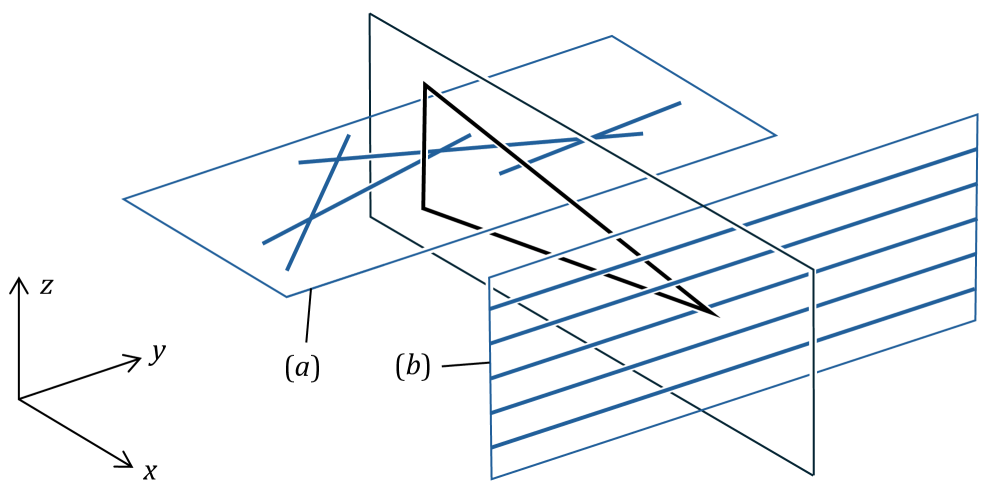
Figure 1: Configuration that achieves $\Omega(n^{2}\alpha(n))$ triple contacts with a triangular robot. The robot is parallel to the $xz$-plane. There is a configuration of $n/2$ obstacle edges parallel to the $xy$-plane that form $\Omega(n\alpha(n))$ lower-envelope intersections, in which the edges are given slightly different $z$-coordinates ($a$). There are another $n/2$ obstacle edges parallel to the $y$-axis with different $z$-coordinates ($b$).

Regarding lower bounds for the complexity of $\mathcal{F}$, a lower bound of $\Omega(n^{2})$ is easy to obtain for any robot. For some types of robots (e.g. a triangle) one can obtain a lower bound of $\Omega(n^{2}\alpha(n))$ (Aronov and Sharir [1]). See Figure 1.

For the two-dimensional case, in which $B$ is a convex polygon free to translate in $\mathbb{R}^{2}$ and the obstacles are polygons with a total of $n$ vertices, the complexity of $\mathcal{F}$ is $O(n)$ (Kedem et al. [6]).

Note that, by affine transformations, the cases where $B$ is a square, or any rectangle or parallelogram, are all equivalent. Similarly, the cases where $B$ is a cube or a box or a parallelepiped are all equivalent.

1.1 Our results

In this paper we prove the following:

Theorem 1.

Let $B$ be a square robot that is free to translate in $\mathbb{R}^{3}$ amidst polyhedral obstacles that have a total of $n$ vertices. Then the complexity of the free space of $B$ is $O(n^{2})$.

As mentioned before, Halperin and Yap proved this bound only when the obstacles are infinite lines.

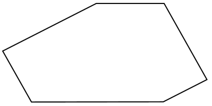
Figure 2: A fully-parallel polygon.

We also study a more general class of polygonal robots. We call a convex polygon fully parallel if its edges come in parallel pairs (not necessarily of the same length). See Figure 2. It is easy to see that the lower bound of $\Omega(n^{2}\alpha(n))$ shown in Figure 1 can be achieved with any polygonal robot that is not fully parallel, as well as with any polyhedral robot that can be projected to form a non-fully-parallel polygon.

On the other hand, if $B$ is a fully-parallel polygon, then the lower bound of Figure 1 does not work: No matter which robot edge makes the double contacts with the obstacle edges of $(a)$, the parallel edge at the opposite end of the robot will not allow the obstacle edges of $(b)$ to be arbitrarily close to each other. We make the following conjecture:

Conjecture 2.

Let $B$ be a fully-parallel convex polygon that is free to translate in $\mathbb{R}^{3}$ amidst polyhedral obstacles that have a total of $n$ vertices. Then the complexity of the free space of $B$ is $O(n^{2})$ (where the hidden constant might depend on $B$).

We managed to prove the following:

Theorem 3.

Let $B$ be a fully-parallel convex polygon that is free to translate in $\mathbb{R}^{3}$ amidst polyhedral obstacles that have a total of $n$ vertices. Then the number of triple contacts not involving three mutually-nonparallel edges of $B$ is $O(n^{2})$ (where the hidden constant depends on $B$).

Hence, the only case remaining in order to prove Conjecture 2 is that of three mutually-nonparallel robot edges.

We obtain a similar partial result for the case where $B$ is a cube (for which the current upper bound is $O(n^{2}\alpha(n))$, and for which the lower bound of Figure 1 does not work):

Theorem 4.

Let $B$ be a cube that is free to translate in $\mathbb{R}^{3}$ amidst polyhedral obstacles that have a total of $n$ vertices. Then the number of triple contacts not involving three mutually-nonparallel edges of $B$ is $O(n^{2})$.

2 Preliminaries

Let $B\subset\mathbb{R}^{3}$ be a polyhedral robot that can translate among a set $\mathcal{C}=\{C_{1},\ldots,C_{k}\}$ of pairwise-disjoint polyhedral obstacles in $\mathbb{R}^{3}$. A placement of $B$ in space can be specified by a point $v$ in configuration space $\mathbb{R}^{3}$. At that placement, the robot occupies the points $B+v=\{b+v:b\in B\}$. Such a placement is free (or legal) if $B+v$ is disjoint from the interior of every obstacle in $\mathcal{C}$. The set of all points in configuration space that correspond to free placements of the robot is called the free space of the robot, which we denote by $\mathcal{F}$.

An observation dating back to Lozano-Pérez and Wesley [7] is that the robot can be replaced by a point if the obstacles are appropriately expanded. Specifically, the free space is given by

$$\mathcal{F}=\mathbb{R}^{3}\setminus\bigcup_{C\in\mathcal{C}}(\operatorname{int}(C)\oplus(-B))$$

where $X\oplus Y=\{x+y:x\in X,y\in Y\}$ denotes the Minkowski sum of two sets of points.

We will assume for simplicity that the obstacles are in general position with respect to the robot, meaning, no obstacle edge is parallel to a robot face, no obstacle face is parallel to a robot edge, etc. It can be shown that such degeneracies can only decrease the complexity of $\mathcal{F}$. (See [1] and references cited there for more details on the general position assumption in the motion planning setting.)

The robot is in contact with an obstacle $C$ in a certain placement if the robot intersects the boundary of $C$ but not its interior in that placement. A contact specification is a pair $O=(f,g)$ where $f$ is a feature (vertex, edge, or face) of the robot, and $g$ is a feature of an obstacle, such that $\dim f+\dim g\leq 2$. A (not necessarily free) placement of the robot is said to realize the contact specification $O$ if at that placement $f$ intersects $g$.

We call the contact specification $O=(f,g)$ generic, singly degenerate, or doubly degenerate, according to whether if $\dim f+\dim g$ equals $2$, $1$, or $0$, respectively. If $O$ is generic, then we call it a vertex contact, an edge contact, or a face contact, according to whether the robot feature $f$ is a vertex, an edge, or a face, respectively.

Due to the general position assumption, each face of $\mathcal{F}$ arises from a connected set of robot placements that realize a fixed generic contact specification.

Similarly, each edge of $\mathcal{F}$ corresponds to a connected set of robot placements that simultaneously realize two generic contact specifications. Some of these edges realize a singly-degenerate contact specification.

Finally, each vertex of $\mathcal{F}$ arises from a robot placement simultaneously realizing three generic contact specifications. See Figure 3 for an example. Some vertices of $\mathcal{F}$ correspond to the robot simultaneously realizing a singly-degenerate contact specification and a generic contact specification, while other vertices of $\mathcal{F}$ correspond to the robot realizing a doubly-degenerate contact specification.

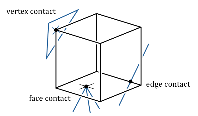
Figure 3: A placement of $B$ (here a cube) making three contacts with obstacles, in this case a vertex contact, an edge contact, and a face contact. This placement of $B$ corresponds to a vertex of the free space.

In order to asymptotically bound the complexity of $\mathcal{F}$, it is enough to bound its number of vertices, since then the same asymptotic bound will also hold for the number of edges and faces. Furthermore, vertices of $\mathcal{F}$ that involve degenerate contact specifications are easily bounded by $O(n^{2})$, so we only need to consider vertices of $\mathcal{F}$ that arise from three generic contact specifications.

3 Upper and lower envelopes

In this section we present some results, some of them new, on upper and lower envelopes, which we will need in subsequent sections.

Let $S$ be a finite collection of graphs of possibly intersecting, possibly partial, functions $\mathbb{R}\to\mathbb{R}$. The lower envelope of $S$ is the pointwise minimum of these function graphs, i.e. the parts of the function graphs that are visible from below at $y=-\infty$. Similarly, the upper envelope of $S$ are the parts of the function graphs that are visible from above at $y=+\infty$.

Hart and Sharir [5] proved that, if $S$ is a collection of nonvertical line segments, then the combinatorial complexity of each envelope of $S$ is at most $O(n\alpha(n))$, where $\alpha(n)$ is the inverse-Ackermann function. In other words, each envelope of $S$ has at most $O(n\alpha(n))$ breakpoints, where a breakpoint could be either a segment endpoint or an intersection of two segments in the envelope. Since there are trivially at most $2n$ segment endpoints, the nontrivial part of this result is that there are at most $O(n\alpha(n))$ intersection points visible from above or below. Furthermore, this bound is worst-case tight (Wiernik and Sharir [8]).

Remark.

Let $S=S_{1}\uplus S_{2}$ be a planar collection of $n$ nonvertical line segments partitioned into two sets. Then the maximum number of lower-envelope intersections between segments of $S_{1}$ and segments of $S_{2}$ is still $\Omega(n\alpha(n))$: Take a configuration $S$ of $n$ segments that realizes the maximum of $\Theta(n\alpha(n))$ lower-envelope intersections. Consider a random partition of $S$ into two parts. Each lower-envelope intersection has a probability of $1/2$ of its two segments falling into different parts. By linearity of expectation, the expected number of lower-envelope intersections between segments of different parts is $\Theta(n\alpha(n)/2)=\Theta(n\alpha(n))$, and there must be a partition that realizes at least this value.

Lemma 5.

Let $S_{1}$ and $S_{2}$ be two collections of nonvertical line segments in the plane with $|S_{1}\cup S_{2}|=n$, such that within each $S_{i}$ no two segments intersect. Then the number intersections between segments of $S_{1}$ and segments of $S_{2}$ that lie in an envelope of $S_{1}$ as well as in an envelope of $S_{2}$ is $O(n)$.

Proof.

Let $x_{1},\ldots,x_{2n}$ be the $x$-coordinates of the endpoints of the segments of $S_{1}\cup S_{2}$ sorted by increasing $x$-coordinate. Within each $x$-range $[x_{i},x_{i+1}]$ the lowest and highest segments of $S_{1}$ are constant, and the lowest and highest segments of $S_{2}$ are constant. These two pairs of segments intersect at most four times, and these are the only intersections that can appear in an envelope of $S_{1}$ as well as in an envelope of $S_{2}$ in this range. ∎

We now strengthen this lemma:

Lemma 6.

Let $S_{1}$ and $S_{2}$ be two collections of nonvertical line segments in the plane with $|S_{1}\cup S_{2}|=n$, such that within $S_{1}$ no two segments intersect (though segments within $S_{2}$ might intersect). (See Figure 4, left.) Then the number intersections between segments of $S_{1}$ and segments of $S_{2}$ that lie in an envelope of $S_{1}$ as well as in an envelope of $S_{2}$ is $O(n)$.

Proof.

Let us bound the number of intersection points of the form $p=s_{1}\cap s_{2}$ where $s_{1}\in S_{1}$, $s_{2}\in S_{2}$, $p$ lies in the lower envelope of $S_{2}$, and $s_{1}$ has a smaller slope than $s_{2}$. Call these intersections relevant. Then all we need to do is multiply the bound on the number of relevant intersections by $4$.

Let us start with the lower relevant intersections, which are the intersections that lie in the lower envelope of $S_{1}$ as well.

Let us ignore the first (leftmost) lower relevant intersection of each segment of $S_{2}$. Hence, we ignore only $O(n)$ lower relevant intersections.

Let $x_{1},\ldots,x_{2m}$ be the $x$-coordinates of the endpoints of the segments of $S_{1}$, sorted by $x$-coordinate. Within each $x$-range $R_{i}=[x_{i},x_{i+1}]$ the lowest segment of $s_{i}\in S_{1}$ is constant.

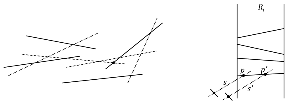
Figure 4: Left: Two collections of segments $S_{1}$, $S_{2}$ in which no two segments of of $S_{1}$ intersect (solid lines), though segments of $S_{2}$ might intersect (dotted lines). The marked intersection lies in the upper envelope of $S_{1}$ and in the lower envelope of $S_{2}$. Right: Since $p$ and $p^{\prime}$ are not the first lower relevant intersections of their corresponding segments $s,s^{\prime}\in S_{2}$, the segments $s$, $s^{\prime}$ must extend to the left of the vertical slab $R_{i}$. But then $s^{\prime}$ passes below $p$.

Within each $x$-range $R_{i}$ there can be at most one non-ignored lower relevant intersection. Indeed, if $s_{i}$ contained two such intersections $p$, $p^{\prime}$, with $p$ left of $p^{\prime}$, then the segment $s^{\prime}\in S_{2}$ that passes through $p^{\prime}$ would have to pass below $p$, obscuring it from below. See Figure 4 (right). Hence, the total number of lower relevant intersections is $O(n)$.

The number of upper relevant intersections (i.e. relevant intersections that lie in the upper envelope of $S_{1}$) is bounded similarly. ∎

4 Triple vertex contacts with a triangular robot

Following Halperin and Yap [4], we first consider the following auxiliary problem: Suppose the robot $B$ is a “flat” triangle that can translate amidst polyhedral obstacles in $\mathbb{R}^{3}$. We would like to bound the number of vertices of the free space $\mathcal{F}$ that correspond to triple vertex contacts, i.e. the number of free placements in which the three vertices of $B$ make contact with three different obstacle faces (see Figure 5). Halperin and Yap derived an upper bound of $O(n^{2}\alpha(n))$ for the number of such contacts. We improve this bound to $O(n^{2})$ by making a minor modification to their argument.

Lemma 7.

Let $B$ be a triangular robot that is free to translate in $\mathbb{R}^{3}$ amidst polyhedral obstacles that have a total of $n$ vertices. Then the number of triple vertex contacts that $B$ can make with obstacles is $O(n^{2})$.

(Recall that if we do not restrict our attention to vertex contacts then $\Omega(n^{2}\alpha(n))$ triple contacts are possible, as shown in Figure 1.)

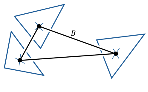
Figure 5: A “flat” triangular robot $B$ in $\mathbb{R}^{3}$ making three vertex contacts.

We now proceed to prove Lemma 7. Suppose without loss of generality that the triangle $B$ is “horizontal”, i.e. parallel to the $xy$-plane. We can assume all obstacle faces are triangles. By the general-position assumption, the vertices of each triangular obstacle face have different $z$-coordinates. Let us split each face into two subtriangles by a horizontal line passing through the vertex with middle $z$-coordinate. Thus, each subtriangle has two non-horizontal sides and one horizontal side.

Let us see what happens to the intersection $f(z_{0})$ between a subtriangle $f$ and a horizontal plane $z=z_{0}$, as we vary $z_{0}$. For every $z_{0}$ in the $z$-range of $f$, $f(z_{0})$ is a line segment. As we increase $z_{0}$ at a constant rate, the line segment moves parallel to itself at constant speed, and its two endpoints also move at constant speed.

4.1 Contact specifications and covering

In our case, the relevant contact specifications are those of the form $O=(p,f)$ where $p$ is a vertex of $B$ and $f$ is a subtriangle.

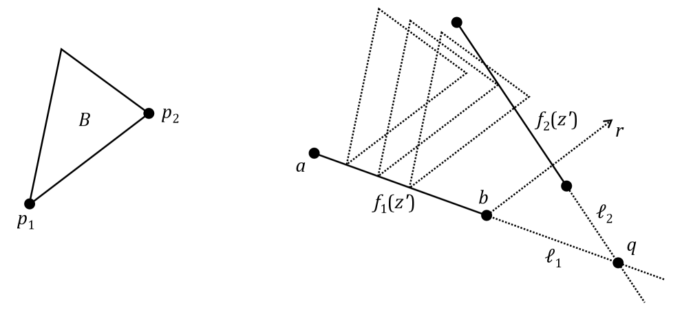
Figure 6: At this value $z=z^{\prime}$, the contact specification $O_{2}=(p_{2},f_{2})$ covers the contact specification $O_{1}=(p_{1},f_{1})$ at the right, since $q$ is to the right of $f_{1}(z^{\prime})$ and the ray $r$ from $b$ with direction $\overrightarrow{p_{1}p_{2}}$ intersects $f_{2}(z^{\prime})$. As we slide the robot $B$ along $f_{1}(z^{\prime})$, it goes from not colliding with $f_{2}(z^{\prime})$ to colliding with it.

Consider two contact specifications $O_{1}=(p_{1},f_{1})$, $O_{2}=(p_{2},f_{2})$, where $p_{1}\neq p_{2}$, and where the $z$-ranges of $f_{1}$, $f_{2}$ overlap. Let $[z_{0},z_{1}]$ be the intersection of the $z$-ranges of $f_{1}$, $f_{2}$. Given $z^{\prime}\in[z_{0},z_{1}]$, we would like to define whether $O_{2}$ covers $O_{1}$ at $z=z^{\prime}$. Let $\ell_{1}=\ell_{1}(z^{\prime})$ and $\ell_{2}=\ell_{2}(z^{\prime})$ be the lines containing the segments $f_{1}(z^{\prime})$ and $f_{2}(z^{\prime})$. Let $q$ be the point of intersection of $\ell_{1}$ and $\ell_{2}$, and suppose that $f_{1}(z^{\prime})$ does not contain $q$. Let $a$, $b$ be the endpoints of $f_{1}(z^{\prime})$, with $a$ left of $b$ (i.e. with smaller $x$-coordinate). Let $r$ be the ray with direction $\overrightarrow{p_{1}p_{2}}$ emerging from the endpoint among $a$, $b$ that is closer to $q$. If $r$ intersects $f_{2}(z^{\prime})$ then we say that $O_{2}$ covers $O_{1}$. If $q$ is to the right of $f_{1}(z^{\prime})$ then we say that $O_{2}$ covers $O_{1}$ at the right; otherwise we say that $O_{2}$ covers $O_{1}$ at the left. See Figure 6.

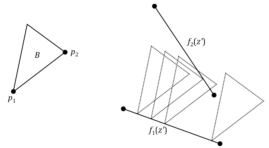
Figure 7: Here $O_{2}=(p_{2},f_{2})$ does not cover $O_{1}=(p_{1},f_{1})$, and as we slide the robot $B$ along $f_{1}(z^{\prime})$, it collides with $f_{2}(z^{\prime})$ but then stops colliding with it.

The significance of $O_{2}$ covering $O_{1}$ is as follows. Suppose we slide the robot with its vertex $p_{1}$ moving along the segment $f_{1}(z^{\prime})$ from one endpoint of $f_{1}(z^{\prime})$ to the other. It might happen that during this motion, the edge $p_{1}p_{2}$ starts colliding with the segment $f_{2}(z^{\prime})$ and then stops colliding with it. See Figure 7. However, if $O_{2}$ covers $O_{1}$ then this is not possible: If the edge $p_{1}p_{2}$ starts colliding with the segment $f_{2}(z^{\prime})$, then the collision will continue until $p_{1}p_{2}$ reaches the other endpoint of $f_{1}(z^{\prime})$.

Since the endpoints of the segments $f_{1}(z^{\prime})$, $f_{2}(z^{\prime})$ move linearly with respect to $z^{\prime}$, the range of values of $z^{\prime}$ at which $O_{2}$ covers $O_{1}$ forms a continuous subinterval of $[z_{0},z_{1}]$.

Consider a placement of the robot realizing three vertex contact specifications $O_{1}=(p_{1},f_{1})$, $O_{2}=(p_{2},f_{2})$, $O_{3}=(p_{3},f_{3})$. For each pair of indices $i,j\in\{1,2,3\}$, $i\neq j$, either $O_{i}$ covers $O_{j}$ or $O_{j}$ covers $O_{i}$. Hence, one of the two following possibilities occurs: Either there is one contact specification that is covered by the other two, or the contact specifications are circular in the sense that $O_{i}$ covers $O_{j}$, $O_{j}$ covers $O_{k}$, and $O_{k}$ covers $O_{i}$. See Figure 8.

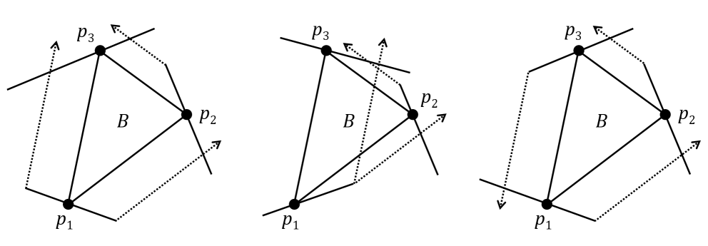
Figure 8: Robot placements realizing three vertex contact specifications $O_{1}$, $O_{2}$, $O_{3}$. In the left and center figures, $O_{1}$ is covered by $O_{2}$ and $O_{3}$. In the right figure, $O_{1}$ is covered by $O_{2}$, which is covered by $O_{3}$, which is covered by $O_{1}$.

4.2 Parametric plane of a contact specification

Given a contact specification $O_{1}=(p_{1},f_{1})$, we define the contact parametric plane $P_{O_{1}}$ in which we parametrize by a pair of real numbers $(z^{\prime},s)$ every robot placement in which the robot vertex $p_{1}$ makes contact with $f_{1}(z^{\prime})$ (or with its supporting line). The number $s$ represents the distance between the left endpoint $a$ of $f_{1}(z^{\prime})$ and the position of $p_{1}$ along $f_{1}(z^{\prime})$. Thus, $P_{O_{1}}\cong\mathbb{R}^{2}$, and the robot placements that realize the contact $O_{1}$ correspond to a triangular region $\Delta_{O_{1}}\subset P_{O_{1}}$. We imagine that the $z$-axis in $P_{O_{1}}$ is horizontal and the $s$-axis is vertical.

We can mark each point of $\Delta_{O_{1}}$ as legal or illegal depending on whether the corresponding robot placement intersects the interior of another obstacle or not.

Given another contact specification $O_{2}=(p_{2},f_{2})$ with $p_{2}\neq p_{1}$, the set of robot placements that realize both $O_{1}$ and $O_{2}$ corresponds either to the empty set or to a line segment within $\Delta_{O_{1}}$. However, we plot in $P_{O_{1}}$ only contact specifications that cover $O_{1}$, and only for the $z$-ranges at which they cover it. Given $O_{2}$ that covers $O_{1}$ at a certain $z$-range, let $\sigma_{O_{2}}$ be the segment in $\Delta_{O_{1}}$ that corresponds to all robot placements that realize the double contact $O_{1}$, $O_{2}$ in this $z$-range. If $O_{2}$ covers $O_{1}$ at the left, then all the points vertically below $\sigma_{O_{2}}$ in the triangle $\Delta_{O_{1}}$ are illegal, and if $O_{2}$ covers $O_{1}$ at the right, then all the points vertically above $\sigma_{O_{2}}$ in $\Delta_{O_{1}}$ are illegal. See Figure 9.

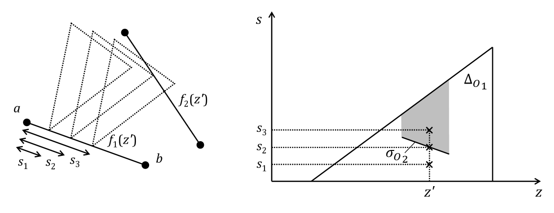
Figure 9: Three robot placements realizing a contact specification $O_{1}$ with the same $z$-value (left); and their representation in the parametric plane $P_{O_{1}}$ (right). The shaded area within $\Delta_{O_{1}}$ represents robot placements that are illegal due to collision with $f_{2}$.

4.3 Families of non-intersecting segments in the parametric planes

Given a contact specification $O_{1}=(p_{1},f_{1})$ and another robot vertex $p_{2}$, let $L_{O_{1},p_{2}}$ (resp. $R_{O_{1},p_{2}}$) be the set of all subtriangles $f$ such that $O_{2}=(p_{2},f)$ covers $O_{1}$ at the left (resp. right) for some range of $z$. For each $f\in L_{O_{1},p_{2}}$ (resp. $R_{O_{1},p_{2}}$) let $\sigma(f)$ be the corresponding line segment in the parametric plane $P_{O_{1}}$. Let $\mathcal{L}_{O_{1},p_{2}}=\{\sigma(f):f\in L_{O_{1},p_{2}}\}$ and $\mathcal{R}_{O_{1},p_{2}}=\{\sigma(f):f\in R_{O_{1},p_{2}}\}$ be the sets of these line segments.

Here is the crucial observation that is missing in [4]: The segments in $\mathcal{L}_{O_{1},p_{2}}$ are pairwise non-intersecting, since if $\sigma(f),\sigma(f^{\prime})\in\mathcal{L}_{O_{1},p_{2}}$ intersected, then the subtriangles $f$, $f^{\prime}$ themselves would intersect. Similarly, the segments in $\mathcal{R}_{O_{1},p_{2}}$ are pairwise non-intersecting.

4.4 Counting triple vertex contacts

We are now ready to bound the number of robot placements making three simultaneous vertex contacts.

Consider first triple contacts in which one contact specification $O_{1}=(p_{1},f_{1})$ is covered by the other two, $O_{2}=(p_{2},f_{2})$, $O_{3}=(p_{3},f_{3})$. In the parametric plane $P_{O_{1}}$, such a triple contact corresponds to the intersection point $q$ of a segment in either $\mathcal{L}_{O_{1},p_{2}}$ or $\mathcal{R}_{O_{1},p_{2}}$ with a segment in either $\mathcal{L}_{O_{1},p_{3}}$ or $\mathcal{R}_{O_{1},p_{3}}$. Furthermore, in order for $q$ to be legal, it is necessary for $q$ to lie in the upper (resp. lower) envelope of $\mathcal{L}_{O_{1},p_{2}}$ (resp. $\mathcal{R}_{O_{1},p_{2}}$), as well as in the upper (resp. lower) envelope of $\mathcal{L}_{O_{1},p_{3}}$ (resp. $\mathcal{R}_{O_{1},p_{3}}$). Hence, Lemma 5 bounds the number of these intersection points $q$, for fixed $O_{1}$, by $O(n)$. Since there are $O(n)$ choices of $O_{1}$, the total bound for this type of triple-intersection contacts is $O(n^{2})$.

Now consider circular triple contacts. Consider a robot placement at $z=z^{\prime}$ realizing the triple contact $O_{1}=(p_{1},f_{1})$, $O_{2}=(p_{2},f_{2})$, $O_{3}=(p_{3},f_{3})$ in which $O_{1}$ is covered by $O_{2}$, $O_{2}$ is covered by $O_{3}$, and $O_{3}$ is covered by $O_{1}$. Say that all the coverings are at the right (the other cases are similar). This robot placement corresponds to a point $q_{1}$ in the segment $\sigma(f_{2})\in\mathcal{R}_{O_{1},p_{2}}$, which is the lowest segment of $\mathcal{R}_{O_{1},p_{2}}$ at $z=z^{\prime}$. The robot placement also corresponds to a point $q_{2}$ in the segment $\sigma(f_{3})\in\mathcal{R}_{O_{2},p_{3}}$, which is the lowest segment of $\mathcal{R}_{O_{2},p_{3}}$. Finally, the robot placement also corresponds to a point $q_{3}$ in the segment $\sigma(f_{1})\in\mathcal{R}_{O_{3},p_{1}}$, which is the lowest segment of $\mathcal{R}_{O_{3},p_{1}}$. All three points $q_{1}$, $q_{2}$, $q_{3}$ have $z$-coordinate equal to $z^{\prime}$.

Consider the lower envelope of $\mathcal{R}_{O_{1},p_{2}}$. This lower envelope is piecewise linear, with breakpoints at discrete values of $z$. Since the segments in $\mathcal{R}_{O_{1},p_{2}}$ are pairwise nonintersecting, each breakpoint is an endpoint of a segment of $\mathcal{R}_{O_{1},p_{2}}$. Let $z_{1}$ be the largest $z$-coordinate of a breakpoint that is smaller than $z^{\prime}$. Define $z_{2}$, $z_{3}$ similarly, by looking at $\mathcal{R}_{O_{2},p_{3}}$, $\mathcal{R}_{O_{3},p_{1}}$, respectively. Let $z^{\prime\prime}=\max\{z_{1},z_{2},z_{3}\}$.

Hence, in the $z$-range $[z^{\prime\prime},z^{\prime}]$ the lowest segment of each $\mathcal{R}_{O_{1},p_{2}}$, $\mathcal{R}_{O_{2},p_{3}}$, $\mathcal{R}_{O_{3},p_{1}}$ is the aforementioned $\sigma(f_{2})$, $\sigma(f_{3})$, $\sigma(f_{1})$, respectively. We charge the triple contact $O_{1}$, $O_{2}$, $O_{3}$ to the breakpoint $z^{\prime\prime}$.

In this charging scheme, each breakpoint in a lower envelope of a parametric plane is charged at most once, because we can reconstruct the triple contact given the breakpoint: Given $z^{\prime\prime}$ which is a breakpoint in $\mathcal{R}_{(p_{1},f_{1}),p_{2}}$, say, we take the segment $\sigma(f_{2})$ that is lowest in $\mathcal{R}_{(p_{1},f_{1}),p_{2}}$ just after $z=z^{\prime\prime}$. Once we know $f_{2}$, we know we need to look at $\mathcal{R}_{(p_{2},f_{2}),p_{3}}$. Then we take the segment $\sigma(f_{3})$ that is lowest in $\mathcal{R}_{(p_{2},f_{2}),p_{3}}$ just after $z=z^{\prime\prime}$. Once we know $f_{3}$, we know we need to look at $\mathcal{R}_{(p_{3},f_{3}),p_{1}}$. Then we take the segment $\sigma(f_{4})$ that is lowest in $\mathcal{R}_{(p_{3},f_{3}),p_{1}}$ just after $z=z^{\prime\prime}$. If $f_{4}=f_{1}$ then we have successfully reconstructed the triple contact-specification $(p_{1},f_{1})$, $(p_{2},f_{2})$, $(p_{3},f_{3})$ (which might or might not be realizable as a triple contact). If $f_{4}\neq f_{1}$ then the breakpoint $z^{\prime\prime}$ we started with does not receive any charge.

Since each breakpoint is a segment endpoint and there are $O(n^{2})$ segments in all the families $\mathcal{R}_{O,p}$ altogether, there are at most $O(n^{2})$ circular triple contacts in which all coverings take place at the right. The other possibilities, in which some of the coverings take place at the left, are treated similarly.

This concludes the proof of Lemma 7.

Remark.

Halperin and Yap [4] defined each $\mathcal{L}_{(p_{1},f_{1}),p_{2}}\cup\mathcal{L}_{(p_{1},f_{1}),p_{3}}$ as a single set, instead of as two separate sets. Therefore, the segments in their sets can intersect, and that is why they got the $\alpha(n)$ factor in their bound. Our approach of defining $\mathcal{L}_{(p_{1},f_{1}),p_{2}}$ and $\mathcal{L}_{(p_{1},f_{1}),p_{3}}$ as two separate sets (and similarly defining $\mathcal{R}_{(p_{1},f_{1}),p_{2}}$ and $\mathcal{R}_{(p_{1},f_{1}),p_{3}}$ as two separate sets) allows us to apply Lemma 5 and get a bound free of the $\alpha(n)$ factor.

Following Halperin and Yap, we conclude the following:

Corollary 8.

Let $B$ be a polyhedral robot of constant complexity that is free to translate in $\mathbb{R}^{3}$ amidst polyhedral obstacles that have a total of $n$ vertices. Then the number of triple vertex contacts that $B$ can make with obstacles is $O(n^{2})$.

Proof.

Every triple contact made by three vertices of $B$ is also a triple contact made by a triangular robot $B^{\prime}$ spanned by those three vertices (though the opposite is not necessarily the case). ∎

5 The case of a square robot

In this section we prove Theorem 1, regarding the case in which $B$ is a “flat” square (or, more generally, a parallelogram). Assume for concreteness that $B$ is a square of side $1$.

In this case, there are three relevant types of contact specifications. The contact specification $O=(f,g)$ is a face contact if $f$ is $B$ itself and $g$ is an obstacle vertex, an edge contact if $f$ is an edge of $B$ and $g$ is an obstacle edge, and a vertex contact if $f$ is a vertex of $B$ and $g$ is an obstacle face.

We will bound by $O(n^{2})$ the number of triple contacts $O_{1}=(f_{1},g_{1})$, $O_{2}=(f_{2},g_{2})$, $O_{3}=(f_{3},g_{3})$ where each $O_{i}$ is of one of these types. We do this by a case analysis.

Lemma 9.

The number of triple contacts in which at least one contact is a face contact is $O(n^{2})$.

Proof.

By the general position assumption, at most one $O_{i}$ can be a face contact. Suppose $O_{1}$ is a face contact. In order to realize $O_{1}$, the robot $B$ is restricted to move in a plane parallel to $B$. As mentioned in the Introduction, in the planar case the complexity of the free space is $O(n)$ [6]. Since there are $O(n)$ choices of $O_{1}$, we get in total at most $O(n^{2})$ triple contacts of this type. ∎

Lemma 10 (Halperin and Yap [4]).

The number of triple contacts in which two contacts involve the same edge of $B$ or two parallel edges of $B$ is $O(n^{2})$.

Proof.

Consider two contact specifications $O_{1}=(f_{1},g_{1})$, $O_{2}=(f_{2},g_{2})$ in which $f_{1}=f_{2}$ or $f_{1}$ and $f_{2}$ are opposite edges of $B$. In order to simultaneously realize $O_{1}$ and $O_{2}$, $B$ is free to move in a line $\ell$ that is parallel to $f_{1}$ and $f_{2}$. When moving along $\ell$, once $B$ makes a third contact specified by $O_{3}=(f_{3},g_{3})$, further movement along $\ell$ will make $B$ intersect $g_{3}$ until $B$ moves distance $1$. But after $B$ moves distance $1$ along $\ell$, it not longer realizes $O_{1}$ nor $O_{2}$. Hence, there are at most two possibilities for $O_{3}$, one for each direction of movement. Since there are $O(n^{2})$ choices for $O_{1}$, $O_{2}$, the claim follows. ∎

We already bounded in Section 4 the case where all three contacts are vertex contacts.

Hence, we only need to bound the case where $O_{1}$ is an edge contact, $O_{2}$ is a vertex contact, and $O_{3}$ is either another vertex contact or an edge contact with $f_{3}$ not parallel to $f_{1}$. For this, we will consider the parametric plane of $O_{1}$.

5.1 Parametric plane of an edge contact

Let $O_{1}=(f_{1},g_{1})$ where $f_{1}$ is an edge of $B$ and $g_{1}$ is an obstacle edge. Assume for concreteness that $f_{1}$ is parallel to the $z$-axis. By the general-position assumption, the obstacle edge $g$ does not have constant $x$-coordinate. Then we can represent each placement of $B$ in which $f_{1}$ (or its extension) intersects $g_{1}$ (or its extension) by a pair $(s,t)$, where $s$ is the distance between the lower-$x$ endpoint of $g_{1}$ and the point of contact $p$, and $t$ is the distance between $p$ and the higher-$z$ endpoint of $f_{1}$.

In the resulting parametric plane $P_{O_{1}}\cong\mathbb{R}^{2}$, the placements in which the contact $O_{1}$ actually takes place correspond to a rectangle $\Gamma=[0,s_{\mathrm{max}}]\times[0,1]\subset P_{O_{1}}$, where $s_{\mathrm{max}}$ is the length of $g_{1}$. Each point of $P_{O_{1}}$ can be marked legal or illegal according to whether the corresponding placement of $B$ is legal or illegal. Consider a second contact specification $O_{2}=(f_{2},g_{2})$, where $f_{2}$ is either a vertex of $B$ or an edge of $B$ not parallel to $f_{1}$. Then the set of points corresponding to placements that realize $O_{2}$ is either empty or a line segment $\sigma_{O_{1},O_{2}}\subset P_{O_{1}}$. Furthermore, the region of $\Gamma$ that is either vertically above or vertically below the segment $\sigma_{O_{1},O_{2}}$ (depending on whether $f_{2}$ lies on the lower-$z$ or the higher-$z$ side of $B$) is illegal. See Figure 10.

Furthermore, if $O_{2}=(f_{2},g_{2})$, $O^{\prime}_{2}=(f_{2},g^{\prime}_{2})$ are vertex contacts involving the same vertex $f_{2}$ of $B$, then the segments $\sigma_{O_{1},O_{2}}$, $\sigma_{O_{1},O^{\prime}_{2}}$ cannot intersect, because then the obstacle faces $g_{2}$, $g^{\prime}_{2}$ would intersect.

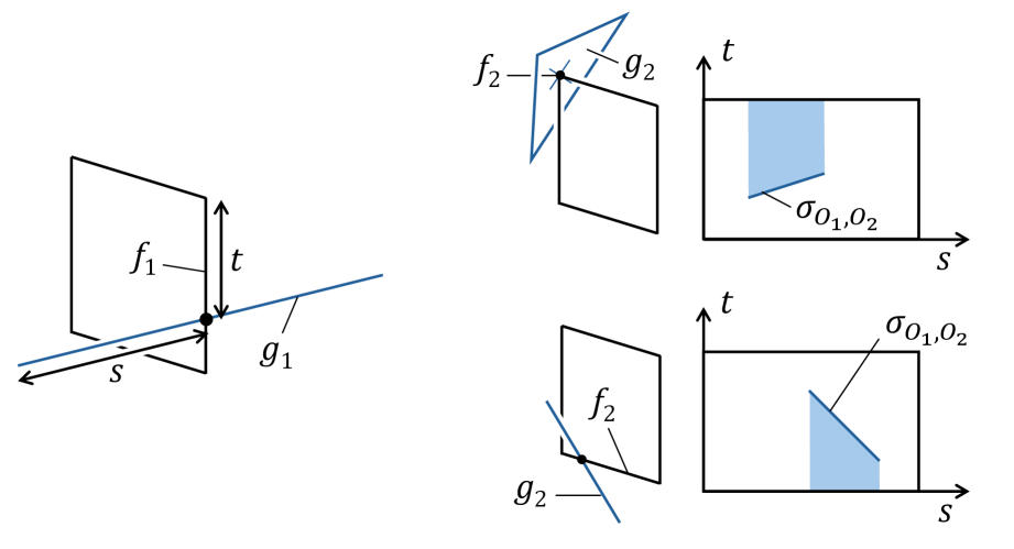
Figure 10: Parametric plane of an edge contact with a square robot. The contact $O_{1}=(f_{1},g_{1})$ defining the parametric plane is shown on the left, and two different options for the second contact $O_{2}=(f_{2},g_{2})$, and the corresponding segments $\sigma_{O_{1},O_{2}}$ in the parametric plane, are shown on the right.

For each $f_{2}$ as above, of dimension $k\in\{0,1\}$, we denote by $S_{O_{1},f_{2}}$ the set of all segments in $P_{O_{1}}$ of the form $\sigma_{O_{1},(f_{2},g_{2})}$ where $g_{2}$ ranges over all obstacle features of dimension $2-k$.

A triple contact $O_{1}$, $O_{2}$, $O_{3}$ then corresponds to an intersection point $p\in P_{O_{1}}$ between a segment in $S_{O_{1},f_{2}}$ and a segment in $S_{O_{1},f_{3}}$. Furthermore, $p$ lies in the lower or the upper envelope of $S_{O_{1},f_{2}}$, as well as in the lower or the upper envelope of $S_{O_{1},f_{3}}$. Moreover, one of the families $S_{O_{1},f_{2}}$, $S_{O_{1},f_{3}}$ consists of pairwise-nonintersecting segments. Hence, by Lemma 6, there are $O(n)$ triple contacts involving $O_{1}$. Multiplying by $O(n)$ choices for $O_{1}$, we get a total of $O(n^{2})$ triple contacts of this form. This finishes the proof of Theorem 1.

6 The case of a fully-parallel polygonal robot

Theorem 3, regarding a fully-parallel polygonal robot, follows by a pair of small modifications to the proof of Theorem 1.

Consider the case where two edge contacts $O_{1}=(f_{1},g_{1})$, $O_{2}=(f_{2},g_{2})$ involve robot edges $f_{1}$, $f_{2}$ that are either equal or parallel. Let $d$ and $D$, with $d<D$, be lengths of $f_{1}$ and $f_{2}$. Then we argue as in the proof of Lemma 10, except that now there are at most $1+\lceil D/d\rceil$ possibilities for $O_{3}$, given $O_{1}$, $O_{2}$. Since this number is a constant, we again get an overall bound of $O(n^{2})$ for this case.

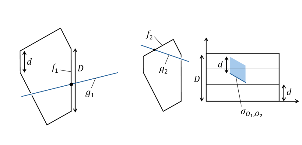
Figure 11: When the robot is a fully-parallel polygon, in the parametric plane of an edge contact $O_{1}$, the parallelogram-shaped region of height $d$ above or below the segment $\sigma_{O_{1},O_{2}}$ is certainly illegal. Hence, we can divide the rectangle into horizontal strips and proceed as before.

Now consider an edge contact $O_{1}=(f_{1},g_{1})$. Let $f^{\prime}_{1}$ be the edge of $B$ that is parallel to $f_{1}$, and let $d$ and $D$ be the smaller and the larger length among $f_{1}$, $f^{\prime}_{1}$, respectively. Consider a second contact $O_{2}=(f_{2},g_{2})$ where $f_{2}$ is either a vertex of $B$ or an edge of $B$ different from $f_{1}$ and $f^{\prime}_{1}$. Consider the segment $\sigma_{O_{1},O_{2}}\in S_{O_{1},f_{2}}$ in the parametric plane $P_{O_{1}}$. Then there is a parallelogram-shaped region of height $d$, either vertically above or vertically below $\sigma_{O_{1},O_{2}}$, that is certainly illegal. See Figure 11. Hence, we can partition the parametric rectangle $\Gamma$ into $\lceil D/d\rceil$ horizontal strips of width at most $d$. This operation might cut some segments in $S_{O_{1},f_{2}}$ into subsegments. Within each strip we are interested only in the lower or the upper envelope of the subsegments in that strip, so we proceed as before.

With these two modifications, Theorem 3 is proven.

7 The case of a cubical robot

We now prove Theorem 4 regarding a cubical (or, more generally, parallelpiped) robot. Assume for concreteness that $B=[0,1]^{3}$ is a unit cube.

Let us go over all types of triple contacts $O_{1}=(f_{1},g_{1})$, $O_{2}=(f_{2},g_{2})$, $O_{3}=(f_{3},g_{3})$.

Lemma 7 already addressed the case of three vertex contacts. Hence, we can assume without loss of generality that $O_{1}$ is not a vertex contact.

Due to the general position assumption, it is impossible to have two face contacts involving the same face or opposite faces of $B$.

If $f_{1}$, $f_{2}$ are the same edge or parallel edges of $B$, then the line of movement of $B$ that preserves these two contacts is parallel to those edges, and hence the argument of Lemma 10 applies. The same is true if $f_{1}$, $f_{2}$ are non-parallel faces of $B$, or if $f_{1}$ is a face of $B$ and $f_{2}$ is an edge of $f_{1}$ or of the face opposite $f_{1}$.

In order to handle the remaining cases, we examine parametric planes of face and edge contacts.

7.1 Parametric plane of a face contact

Let $O_{1}=(f_{1},g_{1})$ be a face contact. The set of all placements of $B$ that realize $O_{1}$ can be parametrized by a pair of real numbers between $0$ and $1$. For example, if the face $f$ is parallel to the $xy$-plane, then we can represent every placement of $B$ that realizes $(f_{1},g_{1})$ by two real numbers $s,t\in[0,1]$, where $s$ denotes the distance from the vertex $g$ to the higher-$x$, $y$-parallel edge of $f$, and $t$ denotes the distance from $g$ to the higher-$y$, $x$-parallel edge of $f$. Real values of $s$ and/or $t$ outside of the range $[0,1]$ give rise to placements in which $g$ lies in the containing plane of $f$, though not in $f$ itself.

In the parametric plane $P_{O_{1}}\cong\mathbb{R}^{2}$, the unit square $\Gamma=[0,1]^{2}\subset P_{O_{1}}$ corresponds to the placements in which the contact $O_{1}$ actually takes place. Each point of $P_{O_{1}}$ can be marked legal or illegal according to whether the corresponding robot placement intersects the interior of some obstacle or not.

As before, given another contact specification $O_{2}=(f_{2},g_{2})$, the set of placements that realize both $O_{1}$ and $O_{2}$ correspond either to a line segment $\sigma_{O_{1},O_{2}}\subset P_{O_{1}}$ or to the empty set.

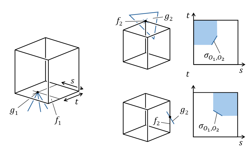
Figure 12: Parametric plane of a face contact for a cube robot.

Whether $O_{2}$ is either an edge contact with $f_{2}$ perpendicular to $f_{1}$, or a vertex contact, the region of $\Gamma$ that lies behind $\sigma_{O_{1},O_{2}}$ in two perpendicular axis-parallel directions is illegal. See Figure 12. Furthermore, if $O_{2}=(f_{2},g_{2})$, $O_{2}^{\prime}=(f_{2},g_{2}^{\prime})$ are two vertex contacts involving the same vertex $f_{2}$ of $B$, then the segments $\sigma_{O_{1},O_{2}}$, $\sigma_{O_{1},O_{2}^{\prime}}$ cannot intersect, because then the obstacle faces $g_{2}$, $g_{2}^{\prime}$ would intersect.

7.2 Parametric plane of an edge contact

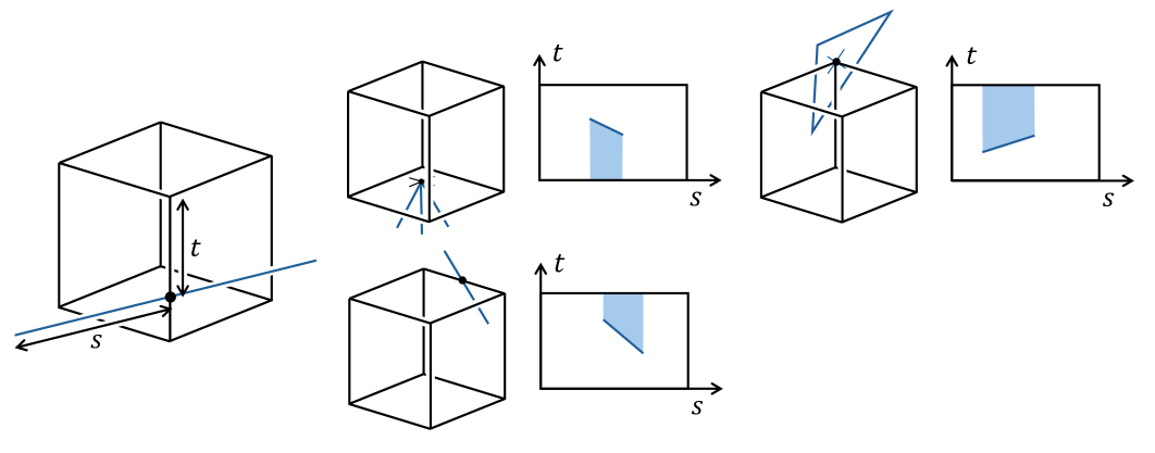
Figure 13: Parametric plane of an edge contact for a cube robot. Conventions are as in previous figures.

Now let $O_{1}=(f_{1},g_{1})$ be an edge contact, and consider a second contact $O_{2}=(f_{2},g_{2})$. As mentioned before, we can assume $f_{2}$ is not an edge parallel to $f_{1}$ nor a face that contains such an edge. Hence, the situation is similar to the one described in Section 5.1. See Figure 13.

7.3 The case analysis

Let us now go over the possibilities not handled by Lemma 7 nor by the argument of Lemma 10.

Suppose at least one contact is a face contact. Say $f_{1}$ is a face of $B$. Then $f_{2}$, $f_{3}$ cannot both be edges of $B$, because then either they would be parallel, or else one of them would belong to $f_{1}$ or to the face opposite $f_{1}$. Thus, one of $f_{2}$, $f_{3}$, say $f_{2}$, must be a vertex of $B$, while $f_{3}$ must be either another vertex of $B$ or an edge perpendicular to $f_{1}$. For each such choice of $f_{1}$, $f_{2}$, $f_{3}$, there are $O(n)$ choices of $g_{1}$. Given a choice of $g_{1}$, consider the parametric plane $P_{O_{1}}$. The segments $\sigma_{O_{1},O_{2}}$, over all choices of $g_{2}$, form a family of segments that do not intersect one another. Hence, we proceed as in Section 5.1, invoking Lemma 6. There are $O(n)$ triple contacts for each choice of $g_{1}$, and hence a total of $O(n^{2})$ contacts involving our choice of $f_{1}$, $f_{2}$, $f_{3}$.

Now suppose no contact is a face contact. At least one contact, say $O_{1}$, must be an edge contact. Hence, let $f_{1}$ be an edge of $B$. Each of $f_{2}$, $f_{3}$ must be an edge or a vertex of $B$, and no two of $f_{1}$, $f_{2}$, $f_{3}$ can be parallel edges. Unless $f_{1}$, $f_{2}$, $f_{3}$ are three mutually nonparallel edges, one of $f_{2}$, $f_{3}$ must be a vertex of $B$. Then Lemma 6 applies again, and we again get a bound of $O(n^{2})$.

Hence, the only case not bounded by $O(n^{2})$ is when $f_{1}$, $f_{2}$, $f_{3}$ are three mutually nonparallel edges of $B$. For such a case, the bound of $O(n^{2}\alpha(n))$ of [4] is still the best bound known. This concludes the proof of Theorem 4.

8 Discussion and open problems

The main open problem is to close the gap between $O(n^{2}\log n)$ and $\Omega(n^{2}\alpha(n))$ for the general case of a convex polyhedral robot. The gap between $O(n^{2}\alpha(n))$ and $\Omega(n^{2})$ for the case of a cubical robot is still open as well. As we showed in this paper, the critical case is the one of triple contacts involving three mutually-nonparallel robot edges.

As we have shown, a similar gap exists when the robot is what we have called a fully parallel polygon. And in this scenario as well, the critical case is the one of triple contacts made by three mutually-nonparallel robot edges.

Another open problem is to obtain more refined bounds that depend on the complexity of the robot, as well as on the number of obstacles, and not just on the total number of obstacle vertices, under the assumption that the obstacles are convex.

Suppose there are $k$ convex obstacles with a total of $n$ vertices. For the general case where the robot is an $r$-vertex polyhedron, Aronov and Sharir [1] proved an upper bound of $O(rnk\log k)$. It is easy to achieve a lower bound of $\Omega(nk)$ for any robot. For a flat triangular robot, the construction of Figure 1 can be modified to achieve $\Omega(nk\alpha(k))$ (see the details in [1]). Halperin (personal communication) derived an upper bound of $O(nk)$ for the case of a segment-shaped robot. These are the currently best known bounds, as far as we know.

Acknowledgements.

Thanks to Danny Halperin for suggesting me to look into this problem and for useful conversations.

References

- [1] Boris Aronov and Micha Sharir. On translational motion planning of a convex polyhedron in 3-space. SIAM Journal on Computing, 26(6):1785–1803, 1997. doi:10.1137/S0097539794266602.
- [2] Dan Halperin, Oren Salzman, and Micha Sharir. Algorithmic motion planning. In Csaba D. Toth, Joseph O’Rourke, and Jacob E. Goodman, editors, Handbook of discrete and computational geometry, pages 1311–1342. Chapman and Hall/CRC, 2017.
- [3] Dan Halperin and Chee-Keng Yap. Combinatorial complexity of translating a box in polyhedral 3-space. In Proceedings of the ninth annual symposium on Computational geometry (SoCG 1993), pages 29–37. ACM, 1993. doi:10.1145/160985.160992.
- [4] Dan Halperin and Chee-Keng Yap. Combinatorial complexity of translating a box in polyhedral 3-space. Computational Geometry, 9(3):181–196, 1998. doi:10.1016/S0925-7721(97)00030-8.
- [5] Sergiu Hart and Micha Sharir. Nonlinearity of Davenport–Schinzel sequences and of generalized path compression schemes. Combinatorica, 6(2):151–177, 1986. doi:10.1007/BF02579170.
- [6] Klara Kedem, Ron Livne, János Pach, and Micha Sharir. On the union of Jordan regions and collision-free translational motion amidst polygonal obstacles. Discrete & Computational Geometry, 1(1):59–71, 1986. doi:10.1007/BF02187683.
- [7] Tomás Lozano-Pérez and Michael A Wesley. An algorithm for planning collision-free paths among polyhedral obstacles. Communications of the ACM, 22(10):560–570, 1979. doi:10.1145/359156.359164.
- [8] Ady Wiernik and Micha Sharir. Planar realizations of nonlinear Davenport-Schinzel sequences by segments. Discrete & Computational Geometry, 3(1):15–47, 1988. doi:10.1007/BF02187894.