New cost terms through the homogenization of an optimal control problem under dynamic boundary conditions on the microscopic particles

Abstract Given an optimal control problem on a heterogeneous body with a periodical structure of particles depending on a small parameter $\varepsilon$, we study the asymptotic behavior, as $\varepsilon\rightarrow 0,$ of the optimal control functional and the optimal state when the initial problem is of parabolic type, and when on the particles’ boundary, we assume a dynamic condition and the actuation of some controls for some subset of the particles. We show, in the so-called “critical case” (concerning a certain relation between the structure’s period, the diameter of the balls, and the growth coefficient of the particles boundary condition), the appearance of some new non-local in time ”strange terms”, not only in the limit parabolic equation but also in the limit cost functional. Microscopic localized controls generate peculiar terms in both the limit equation and the cost functional that do not appear in the case of controls applied to the entire set of particles or when the boundary condition on the particles is of Robin type.

Keywords Homogenization, Critical case, optimal control, Strange term, Dynamic boundary condition, homogenized cost functional.
Subject Classification 35B27, 35K20, 49K20, 93C20.

1. Introduction

The problem we will consider arises in many different fields. For instance, it is well-known that many problems in Chemical Engineering lead to the optimization of some cost functionals ([29], [22]) and the same happens in the Porous Media Theory in which the word “particle” must be replaced by “perforation” (see, e.g. [18], [17], [4], [23], [16], [19], [27], [1] and the many other references quoted in the monographs [6]). Simplified models in Climatology can be also modeled in terms very close to the ones we will study in this paper ([11]).

The main goal of this paper is to illustrate how the homogenization of some optimal control problems may give rise to new non-local in time ”strange terms”, not only in the limit parabolic equation but also in the limit cost functional, assuming a dynamic boundary condition and the actuation of some controls on some subset of the particles. We will do that for the so-called “critical case”, that is characterized by certain relation between the structure’s period, the diameter of the balls, and the growth coefficient in the particles’ boundary condition. In this way, microscopic localized controls generate peculiar terms in both the limit equation and the cost function that do not appear, for instance, in the case of the Robin type boundary condition on the particles.

We give a detailed presentation of the heterogeneous domain $\Omega_{\varepsilon}$ in the next Section, but for the moment, we outline that, since in the most of the cases it is impossible to act over the entire spatial domain $\Omega_{\varepsilon}$, the control is applied only on the boundary of the particles contained in a small portion of the domain ($\omega$ such that $\overline{\omega}\subset\Omega$). Thus, the set of boundaries of the internal particles is constituted in the form $S_{\varepsilon}=S_{\varepsilon}^{1}\bigcup S_{\varepsilon}^{2}$, where $S_{\varepsilon}^{2}$ is the set of boundaries of the controlling particles $G_{\varepsilon}^{2}$ and $S_{\varepsilon}^{1}$ is the set of boundaries of the particles $G_{\varepsilon}^{1}$ to which no control is implemented. The state of the control problem is given through

$$\left\{\begin{array}[]{lr}\partial_{t}u_{\varepsilon}(v)-\Delta u_{\varepsilon}(v)=f,&(x,t)\in Q_{\varepsilon}^{T},\\ \varepsilon^{-\gamma}\partial_{t}u_{\varepsilon}(v)+\partial_{\nu}u_{\varepsilon}(v)=\varepsilon^{-\gamma}\chi_{S_{\varepsilon}^{2,T}}v,&(x,t)\in S_{\varepsilon}^{T},\\ u_{\varepsilon}(v)(x,0)=0,&x\in\Omega_{\varepsilon}\bigcup S_{\varepsilon},\\ u_{\varepsilon}(v)(x,t)=0,&(x,t)\in\Gamma^{T},\end{array}\right.$$ (1)

where $f\in L^{2}(Q^{T})$ and $v\in L^{2}(S_{\varepsilon}^{2,T})$ is the control. Here, we are using the notation (considering $0<T<\infty$)

$$\begin{array}[]{llll}\Omega_{\varepsilon}=\Omega\setminus\overline{G_{\varepsilon}},&S_{\varepsilon}=\partial G_{\varepsilon},&\partial\Omega_{\varepsilon}=S_{\varepsilon}\cup\partial\Omega,&\\ Q_{\varepsilon}^{T}=\Omega_{\varepsilon}\times(0,T),&\Gamma^{T}=\partial\Omega\times(0,T),&S_{\varepsilon}^{T}=S_{\varepsilon}\times(0,T),&Q^{T}=\Omega\times(0,T),\end{array}$$ (2)

which will be described in detail in the next section. We note that $G_{\varepsilon}$ is the set of small particles ( $\varepsilon$-periodically distributed and homothetic to a unit ball $G_{0}$) in an open bounded regular set $\Omega$ of $\mathbb{R}^{n}$, $n\geq 3$. By $\chi_{S_{\varepsilon}^{2,T}}$, we denote the characteristic function of the set $S_{\varepsilon}^{2,T}=S_{\varepsilon}^{2}\times(0,T)$ that lies entirely in the set $\omega_{\varepsilon}^{T}$ defined below

$$\omega_{\varepsilon}=\omega\cap\Omega_{\varepsilon},\quad\omega_{\varepsilon}^{T}=\omega_{\varepsilon}\times(0,T),\quad\omega^{T}=\omega\times(0,T).$$

The parameter $\gamma>0$ plays a crucial role since in this paper we consider the so-called “critical case” governed by the size of particles that are translations of a small particle $a_{\varepsilon}G_{0},$ where $G_{0}$ is the unit ball with radious $a_{\varepsilon}=C_{0}\varepsilon^{\gamma}$, $\gamma=\frac{n}{n-2},$ and $C_{0}$ is some positive constant.

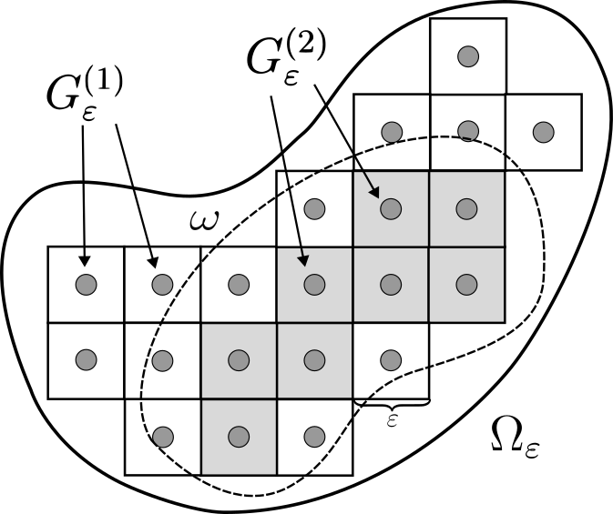
Figure 1. Perforated domain. The control is implemented only on $S_{\varepsilon}^{2}$, the boundary of some of the internal balls: the ones collected under the $G^{2}_{\varepsilon}$.

Notice that since the problem (1) is linear, by some obvious change of variable, we can also consider the case of a non-zero initial datum. To finalize the statement of the optimal control problem, we introduce the cost functional $J_{\varepsilon}:L^{2}(0,T;L^{2}(S_{\varepsilon}^{2}))\rightarrow\mathbb{R}$

$$J_{\varepsilon}(v)=\frac{1}{2}\|\nabla{u_{\varepsilon}(v)}\|_{L^{2}(Q_{\varepsilon}^{T})}^{2}+\frac{1}{2}\int\limits_{\Omega_{\varepsilon}}u_{\varepsilon}^{2}(v)(x,T)dx\\ +\frac{{\varepsilon}^{-\gamma}}{2}\int\limits_{S_{\varepsilon}}u_{\varepsilon}^{2}(v)(x,T){ds}+\varepsilon^{-\gamma}\frac{N}{2}\|{v}\|_{L^{2}(S_{\varepsilon}^{2,T})}^{2},$$ (3)

where $N>0$. Then, the optimal control $v_{\varepsilon}$ is given by

$$J_{\varepsilon}(v_{\varepsilon})=\inf\limits_{v\in L^{2}(0,T;L^{2}(S_{\varepsilon}^{2}))}J_{\varepsilon}(v).$$ (4)

In what follow, we will abuse the notation and simply write $u_{\varepsilon}$ instead of $u_{\varepsilon}(v_{\varepsilon})$. By applying different results in the literature (see, e.g., [21], [14], [28], [15]), it is well-known that there exists a unique optimal control $v_{\varepsilon}\in L^{2}(0,T;L^{2}(S_{\varepsilon}^{2}))$.

We point out that the consideration of a non-zero target function $u_{T}\in L^{2}(\Omega_{\varepsilon})$, a given profile observed at the final time $T$, can be reduced to the above case of $u_{T}\equiv 0$ by a suitable change of variables, at least for a dense set of $u_{T}$ in $L^{2}(\Omega)$ (see Remark 1 below).

The main goal of this paper is to apply a homogenization process to the above optimal control problem when $\varepsilon\rightarrow 0$. As in many other formulations, the kind of the limit problem strongly depends on the size of the particles’ radii $C_{0}\varepsilon^{\alpha}$, $C_{0}>0$ (see, e.g. [27], [1] and the exposition made in [6]). Here, we consider the critical case in which $\alpha=\gamma={n}/{(n-2).}$ For different elliptic and parabolic problems, it is well-known that this critical choice leads to the emergence of a new local “strange” term (the naming is due to [3]) in the effective partial differential equation (see [18], [3], [20], [30], and the monograph [6]).

It is well-known that the introduction of a dynamic boundary condition on the particle boundary causes the aforementioned “strange” term to become a “non-local” operator, derived by solving a suitable ordinary differential equation (we refer to [5], [13], for the case of an elliptic Poisson equation for the state). Also, it was shown that in the framework of optimal control problems there appear some new terms in the limit cost functional (in contrast with previous results in the literature for related formulations, (see, e.g., [25], [31], [24], [26], [7], [8], [9] and especially [12] for the case of distributed controls appearing in the state equation). One of the major new features we will demonstrate in this article is that when the controls act on the boundary of some particles, some new terms appear in the cost functional, the non-local terms in time are of a different nature and some new non-local in time operators must be introduced.

To state the homogenization results, we need to introduce several auxiliary problems. On the uncontrolled particles, we use non-local operator $M(\varphi)$, arising in previous studies (see [12]), that is defined as a solution to

$$\left\{\begin{array}[]{lr}\partial_{t}M(\varphi)+\mathcal{B}_{n}M(\varphi)=\varphi,&t\in(0,T),\\ M(\varphi)(0)=0,&\end{array}\right.$$ (5)

where $\mathcal{B}_{n}=(n-2)C_{0}^{-1}$ and $\varphi\in L^{2}(0,T)$ is a given function, and its adjoint operator $M^{\ast},$

$$\left\{\begin{array}[]{lr}-\partial_{t}M^{\ast}(\varphi)+\mathcal{B}_{n}M^{\ast}(\varphi)=\varphi,&t\in(0,T),\\ M^{\ast}(\varphi)(T)=0.&\end{array}\right.$$ (6)

A similar non-local operator, $G(\varphi)$, and its adjoint operator $G^{\ast},$ must be defined on the controlled particles

$$\left\{\begin{array}[]{lr}\partial_{t}G(\varphi)+(\mathcal{B}_{n}+N^{-1})G(\varphi)=\varphi,&t\in(0,T),\\ G(\varphi)(0)=0,\quad&\end{array}\right.$$ (7)

$$\left\{\begin{array}[]{lr}-\partial_{t}G^{\ast}(\varphi)+(\mathcal{B}_{n}+N^{-1})G^{\ast}(\varphi)=\varphi,&t\in(0,T),\\ G^{\ast}(\varphi)(T)=0.&\end{array}\right.$$ (8)

Besides that, we will need to define some new operators $H$ and $H^{\ast},$ coupled with $G^{\ast}$ and $G,$ respectively, by the problems

$$\left\{\begin{array}[]{lr}-\partial_{t}H^{\ast}(\varphi)+(\mathcal{B}_{n}+N^{-1})H^{\ast}(\varphi)-N^{-1}(\mathcal{B}_{n}+N^{-1})G(H^{\ast}(\varphi))=\varphi,&t\in(0,T),\\ H^{\ast}(\varphi)(T)=0,&\end{array}\right.$$ (9)

and

$$\left\{\begin{array}[]{lr}\partial_{t}H(\varphi)+(\mathcal{B}_{n}+N^{-1})H(\varphi)-N^{-1}(\mathcal{B}_{n}+N^{-1})G^{\ast}(H(\varphi))=\varphi,&t\in(0,T),\\ H(\varphi)(0)=0.&\end{array}\right.$$ (10)

Notice that the operators $G,$ $M,$ $G^{\ast}$ and $M^{\ast}$ can be explicitly written. For instance

$$G(\varphi)(t)=\int\limits_{0}^{t}e^{-(\mathcal{B}_{n}+N^{-1})(t-s)}\varphi(s)ds,$$

which show the non-local in time nature. Some useful properties of these operators will be shown later (see Section 4).

Although, the detailed statements of our results will be presented later, we summarize now that we will prove the convergence of the optimal controls $v_{\varepsilon}$ $\chi_{S_{\varepsilon}^{2,T}}\rightarrow v_{0}\chi_{\omega^{T}}$ strongly in $L^{2}(\omega^{T})$, the convergence of the corresponding states (extended to $\Omega$) $\tilde{u}_{\varepsilon}\rightharpoonup u_{0}$ weakly in $L^{2}(0,T;H_{0}^{1}(\Omega,\partial\Omega))$ and $\partial_{t}\tilde{u}_{\varepsilon}\rightharpoonup\partial_{t}u_{0}$ weakly in $L^{2}(Q^{T})$, and in some sense, that will be indicated later, the microscopic optimal control $v_{\varepsilon}$ converges to the macroscopic optimal control $v_{0}\in H^{1}(0,T;L^{2}(\omega)),$ with the limit state problem given by

$$\left\{\begin{array}[]{ll}\partial_{t}u_{0}(v)-\Delta u_{0}(v)+\mathcal{A}_{n}(u_{0}(v)-\mathcal{B}_{n}H(u_{0}(v)))\chi_{\omega^{T}}&\\ +\mathcal{A}_{n}(u_{0}(v)-\mathcal{B}_{n}M(u_{0}(v)))\chi_{(\Omega\setminus\overline{\omega})\times(0,T)}=f+\mathcal{A}_{n}\mathcal{B}_{n}v\chi_{\omega^{T}},&(x,t)\in Q^{T},\\ u_{0}(v)(x,0)=0,&x\in\Omega,\\ u_{0}(v)(x,t)=0,&(x,t)\in\Gamma^{T},\end{array}\right.$$ (11)

where $v\in H^{1}(0,T;L^{2}(\omega))$ with $v(x,0)=0$ and the limit cost functional given by

$$J_{0}(v) = \|\nabla u_{0}(v)\|_{L^{2}(Q^{T})}^{2}+\|u_{0}(v)(x,T)\|_{L^{2}(\Omega)}^{2}+N^{-1}\mathcal{A}_{n}\mathcal{B}_{n}\int\limits_{\omega^{T}}(\partial_{t}G^{\ast}(H(u_{0}(v))))^{2}{dxdt}$$ (12)

$$+\mathcal{A}_{n}\mathcal{B}_{n}\int\limits_{\Omega\setminus\overline{\omega}}|M(u_{0}(v))(x,T)|^{2}{dx}+\mathcal{A}_{n}\int\limits_{(\Omega\setminus\overline{\omega})\times(0,T)}|u_{0}(v)-\mathcal{B}_{n}M(u_{0}(v))|^{2}{dxdt}$$

$$+\mathcal{A}_{n}\mathcal{B}_{n}\int\limits_{\omega}|H(u_{0}(v))(x,T)|^{2}{dx}+\mathcal{A}_{n}\int\limits_{\omega^{T}}|u_{0}(v)-\mathcal{B}_{n}H(u_{0}(v))|^{2}{dxdt}$$

$$+N\mathcal{A}_{n}\mathcal{B}_{n}\int\limits_{\omega^{T}}(\partial_{t}v)^{2}{dxdt}+\mathcal{A}_{n}\mathcal{B}_{n}(\mathcal{B}_{n}+N^{-1})\int\limits_{\omega}v^{2}(x,T){dx}+$$

$$+N\mathcal{A}_{n}\mathcal{B}_{n}^{2}(\mathcal{B}_{n}+N^{-1})\int\limits_{\omega^{T}}v^{2}{dxdt}.$$

of the optimal control problem

$$J_{0}(v_{0})=\min\limits_{v\in U_{ad}}J_{0}(v),$$ (13)

where the set of admissible functions is now

$$U_{ad}=\{\psi\in H^{1}(0,T;L^{2}(\omega))|\psi(x,0)=0\}.$$

It can be seen that the first two terms and the last term of $J_{0}$ clearly correspond to the three terms present in $J_{\varepsilon}$, but the rest of the terms of $J_{0}$ are, in some way, unexpected. The terms of $J_{0}$ which are related to the final evaluation at time $T$ are new, and two of them are actually non-local in time since they involve the operators $M$ and $H$, respectively. The terms of $J_{0}$ which contain the operator $M$ are integrals extended on the complementary of $\omega$, and they are a consequence of the microscopic control $v_{\varepsilon}$ being applied only at the boundary of some particles, $S_{\varepsilon}^{2},$ and not at all of them. The unexpected terms of $J_{0}$ appear as a consequence of several implicit relations that are justified in the proof of the Theorem 3 below. The last set of the terms that affect time derivatives of a function of $u_{0}$ and the control $v$ are very surprising since nothing suggests their appearance when observing the expression for $J_{\varepsilon}.$

In order to get the proof of these convergence results, we will use the extension of the Pontryagin’s method to the case of boundary controls (see, e.g., [21]). In Section 2, we give the details of the formulation of the direct problem as well the coupled system arising in terms of the adjoint optimal state $p_{\varepsilon}$: we will show that the optimal control is given by $v_{\varepsilon}=-N^{-1}p_{\varepsilon}\chi_{S_{\varepsilon}^{2,T}}.$ The a priori estimates allow passing to the limit in the couple $(u_{\varepsilon},p_{\varepsilon})$ (and thus in the controls $v_{\varepsilon}$) are obtained in Section 3. Some detailed statements of the main theorems of this paper are collected in Section 5, but before that, we present in Section 4 some properties of the auxiliary non-local in time operators $G$, $H$ and $M$ defined above. The proof characterizing the limit couple $(u_{0},p_{0})$ from the microscopic couple $(u_{\varepsilon},p_{\varepsilon})$ is given in Section 6. Finally, the identification of the limit cost functional $J_{0}(v)$ from the microscopic cost functional $J_{\varepsilon}(v)$ is obtained in Section 7.

2. Problem statement and the adjoint problem

Let $\Omega$ be a bounded domain in $\mathbb{R}^{n}$, $n\geq 3$, with a smooth boundary $\partial\Omega$. We denote the unit cube $(-1/2,1/2)^{n}$ centered at the coordinates origin as $Y$. Let $G_{0}$ be a ball of radii $C_{0}$ such that $\overline{G}_{0}\subset Y$. Next, given a set $B$ of $\mathbb{R}^{n},$ by $\delta B$, $\delta>0$, we denote the set $\{x\in\mathbb{R}^{n}|\delta^{-1}x\in B\}$. For $\varepsilon>0$, we define $\widetilde{\Omega}_{\varepsilon}=\{x\in\Omega|\rho(x,\partial\Omega)>2\varepsilon\}$, where $\rho$ is the Euclidean distance. Let $a_{\varepsilon}=C_{0}\varepsilon^{\alpha}$, where $C_{0}$ is a positive constant and $\alpha=\frac{n}{n-2}$. We define sets $G_{\varepsilon}^{j}=a_{\varepsilon}G_{0}+j$, where $j\in\mathbb{Z}^{n}$, $\mathbb{Z}^{n}$ is the set of vectors in $\mathbb{R}^{n}$ with integer coordinates. Now, we introduce the set of indices $\Upsilon_{\varepsilon}=\{j\in\mathbb{Z}^{n}:(a_{\varepsilon}G_{0}+{\varepsilon}j)\bigcap\widetilde{\Omega_{\varepsilon}}\neq\emptyset\}$, note that the cardinal of $\Upsilon_{\varepsilon}$ satisfies that $|\Upsilon_{\varepsilon}|\cong d{\varepsilon}^{-n}$ for some $d=const>0$. Finally, we define the set

$$G_{\varepsilon}=\bigcup_{j\in\Upsilon_{\varepsilon}}G_{\varepsilon}^{j}.$$

Now, if we define $Y_{\varepsilon}^{j}={\varepsilon}Y+{\varepsilon}j$, $P_{\varepsilon}^{j}={\varepsilon}j$, where $Y=(-1/2,1/2)^{n}$, then it is easy to see that $\overline{G_{\varepsilon}^{j}}\subset Y_{\varepsilon}^{j}$ and the center of the ball $G_{\varepsilon}^{j}=a_{\varepsilon}G_{0}+{\varepsilon}j$ coincides with the center of the cube $Y_{\varepsilon}^{j}$.

In the formulation of the optimal control problem, we will consider only some controllable region $\omega$, $\overline{\omega}\subset\Omega$, in the whole domain $\Omega$. Thus, we split indices of $\Upsilon_{\varepsilon}$ into two subsets $\Upsilon^{2}_{\varepsilon}=\{j\in\Upsilon_{\varepsilon}:\overline{Y^{j}_{\varepsilon}}\subset\omega\}$ and $\Upsilon^{1}_{\varepsilon}=\Upsilon_{\varepsilon}\setminus\Upsilon^{2}_{\varepsilon}$. Based on these sets, we will use the following notations

$$G_{\varepsilon}^{1}=\bigcup_{j\in\Upsilon^{1}_{\varepsilon}}{G^{j}_{\varepsilon}},\,G_{\varepsilon}^{2}=\bigcup_{j\in\Upsilon^{2}_{\varepsilon}}{G^{j}_{\varepsilon}},$$

$$S^{1}_{\varepsilon}=\partial G^{1}_{\varepsilon},\,S^{2}_{\varepsilon}=\partial G^{2}_{\varepsilon}.$$

Further, we introduce the sets

$$\Omega_{\varepsilon}=\Omega\setminus\overline{G_{\varepsilon}},\quad\partial\Omega_{\varepsilon}=\partial\Omega\cup S_{\varepsilon},\quad S_{\varepsilon}=S_{\varepsilon}^{1}\cup S_{\varepsilon}^{2},$$

and, for $0<T<\infty$, we define

$$Q^{T}_{\varepsilon}=\Omega_{\varepsilon}\times(0,T),\,\,\omega^{T}=\omega\times(0,T),$$

$$S_{\varepsilon}^{T}=S_{\varepsilon}\times(0,T),\,S_{\varepsilon}^{i,T}=S_{\varepsilon}^{i}\times(0,T),\,i=1,2.$$

Now, we are in a position to formulate optimal control problem. Let $v\in L^{2}(0,T;S_{\varepsilon}^{2})$. By $u_{\varepsilon}(v)$, we denote an element of $L^{2}(0,T;H^{1}(\Omega_{\varepsilon},\partial\Omega))$ with the time derivative satisfying $\partial_{t}u_{\varepsilon}(v)\in L^{2}(0,T;L^{2}(\Omega_{\varepsilon}))\bigcap L^{2}(0,T;L^{2}(S_{\varepsilon}))$ and $u_{\varepsilon}(x,0)=0$ for $x\in\Omega_{\varepsilon}\bigcup S_{\varepsilon}$, that is a solution to the parabolic problem with the internal dynamic boundary condition. By $H^{1}(\Omega_{\varepsilon},\partial\Omega)$, we denote the closure with respect to the norm $H^{1}(\Omega_{\varepsilon})$ of the set of infinitely differentiable in $\overline{\Omega}_{\varepsilon}$ functions vanishing near the boundary $\partial\Omega$. As a solution of (1), we will consider a function $u_{\varepsilon}(v)$ with the above-mentioned properties that satisfies the following integral identity

$$\int\limits_{Q_{\varepsilon}^{T}}\partial_{t}u_{\varepsilon}\varphi{dxdt}+\int\limits_{Q_{\varepsilon}^{T}}\nabla u_{\varepsilon}\nabla\varphi{dxdt}+\varepsilon^{-\gamma}\int\limits_{S_{\varepsilon}^{T}}\partial_{t}u_{\varepsilon}\varphi{dsdt}=\int\limits_{Q_{\varepsilon}^{T}}f\varphi{dxdt}+\varepsilon^{-\gamma}\int\limits_{S_{\varepsilon}^{2,T}}v\varphi{dsdt}$$ (14)

for an arbitrary function $\varphi\in L^{2}(0,T;H^{1}(\Omega_{\varepsilon},\partial\Omega))$. We consider now the optimal control problem stated in the Introduction (see (4)).

Remark 1.

Our approach can be easily extended to the case of a non-zero target $u_{T}\in L^{2}(\Omega)$, at least for a dense set of $u_{T}$ in $L^{2}(\Omega)$, i.e. the cost functional will be

$$J_{\varepsilon}(v) = \frac{1}{2}\|\nabla{u_{\varepsilon}(v)}\|_{L^{2}(Q_{\varepsilon}^{T})}^{2}+\frac{1}{2}\int\limits_{\Omega_{\varepsilon}}\left(u_{\varepsilon}(v)(x,T)-u_{T}\right)^{2}dx$$ (15)

$$+\frac{{\varepsilon}^{-\gamma}}{2}\int\limits_{S_{\varepsilon}}u_{\varepsilon}^{2}(v)(x,T){ds}+\varepsilon^{-\gamma}\frac{N}{2}\|{v}\|_{L^{2}(S_{\varepsilon}^{2,T})}^{2}.$$

Indeed, let us assume that $u_{T}\in L^{2}(\Omega)$ is such that there exists a converging as $\varepsilon\to 0$ sequence of functions $V_{\varepsilon}\in L^{2}(0,T;L^{2}(\Omega_{\varepsilon}))$, i.e.

$$V_{\varepsilon}\rightharpoonup V_{0}\mbox{ weakly in }L^{2}(Q^{T}),\text{ for some }V_{0}\in L^{2}(Q^{T}),$$ (16)

such that for the unique solution $U_{\varepsilon}$ of the auxiliary problem

$$\left\{\begin{array}[]{lr}\partial_{t}U_{\varepsilon}-\Delta U_{\varepsilon}=V_{\varepsilon},&(x,t)\in Q_{\varepsilon}^{T},\\ \varepsilon^{-\gamma}\partial_{t}U_{\varepsilon}+\partial_{\nu}U_{\varepsilon}=0,&(x,t)\in S_{\varepsilon}^{T},\\ U_{\varepsilon}(x,0)=0,&x\in\Omega_{\varepsilon}\bigcup S_{\varepsilon},\\ U_{\varepsilon}(x,t)=0,&(x,t)\in\Gamma^{T},\end{array}\right.$$ (17)

we have

$$\widetilde{U}_{\varepsilon}\rightharpoonup U_{0}\mbox{ weakly in }L^{2}(0,T;H_{0}^{1}(\Omega)),\\ \partial_{t}\widetilde{U}_{\varepsilon}\rightharpoonup\partial_{t}U_{0}\mbox{ weakly in }L^{2}(Q^{T}),$$ (18)

and

$$U_{0}(x,T)=u_{T}(x)\,\text{ a.e. }\,x\in\Omega.$$

Then by defining the change of variables

$$w{{}_{\varepsilon}(v)=u_{\varepsilon}(v)-}U_{\varepsilon},$$

where now ${u_{\varepsilon}(v)}$ is the optimal control associated to the cost functional (15), we find that $w{{}_{\varepsilon}(v)}$ is the optimal control associate to the previous cost functional (3) with $u_{T}\equiv 0.$ Finally, by the arguments of Remark 7.1 of [12] (or Theorem 4 of [11]), it is easy to prove that the set of final data $u_{T}\in L^{2}(\Omega)$ satisfying the above mentioned conditions is a dense set of $L^{2}(\Omega).$ Then, the perturbed equation satisfied by $w{{}_{\varepsilon}(v)}$, i.e.

$$\partial_{t}w{{}_{\varepsilon}(v)}-\Delta w{{}_{\varepsilon}(v)}=f-V_{\varepsilon},$$

does not add any difficulty, once we know that (16) holds.

To obtain the characterization of the optimal control, we consider the adjoint problem

$$\left\{\begin{array}[]{lr}-\partial_{t}p_{\varepsilon}-\Delta p_{\varepsilon}=-\Delta u_{\varepsilon},&(x,t)\in Q_{\varepsilon}^{T},\\ \partial_{\nu}p_{\varepsilon}-\varepsilon^{-\gamma}\partial_{t}p_{\varepsilon}=\partial_{\nu}u_{\varepsilon},&(x,t)\in S_{\varepsilon}^{T},\\ p_{\varepsilon}(x,T)=u_{\varepsilon}(x,T),&x\in\Omega_{\varepsilon}\bigcup S_{\varepsilon},\\ p_{\varepsilon}(x,t)=0,&(x,t)\in\Gamma^{T}.\end{array}\right.$$ (19)

We say that a function $p_{\varepsilon}\in L^{2}(0,T;H^{1}(\Omega_{\varepsilon},\partial\Omega)),$ with $\partial_{t}p_{\varepsilon}\in L^{2}(0,T;L^{2}(\Omega_{\varepsilon}))\cap L^{2}(0,T;L^{2}(S_{\varepsilon})),$ is a weak solution to the problem (19) if $p_{\varepsilon}(x,T)=u_{\varepsilon}(x,T)$ for a.e. $x\in\Omega_{\varepsilon}$ and a.e. $x\in S_{\varepsilon}$ and if it satisfies the integral identity

$$-\int\limits_{Q_{\varepsilon}^{T}}\partial_{t}p_{\varepsilon}\varphi{dxdt}+\int\limits_{Q_{\varepsilon}^{T}}\nabla p_{\varepsilon}\nabla\varphi{dxdt}-\varepsilon^{-\gamma}\int\limits_{S_{\varepsilon}^{T}}\partial_{t}p_{\varepsilon}\varphi{dsdt}=\int\limits_{Q_{\varepsilon}^{T}}\nabla u_{\varepsilon}\nabla\varphi{dxdt},$$ (20)

for any test function $\varphi\in L^{2}(0,T;H^{1}(\Omega_{\varepsilon},\partial\Omega))$. For a given $u_{\varepsilon}$ (with the regularity of the weak solutions of (1)) it is well-known that there exists a unique solution to the problem (19) (see, e.g., [2] and its references).

The following theorem gives a characterization of the optimal control $v_{\varepsilon}$ in terms of the adjoint state $p_{\varepsilon}$.

Theorem 1.

Let the pair of functions $(u_{\varepsilon}(v_{\varepsilon}),v_{\varepsilon})$ be an optimal solution of the problem (4), then $v_{\varepsilon}=-N^{-1}p_{\varepsilon}\chi_{S^{2,T}_{\varepsilon}}$, where $p_{\varepsilon}$ is the solution to (19). The converse is also true.

Proof.

Let $v$ be an arbitrary function in $L^{2}(S^{2,T}_{\varepsilon})$ and $\lambda>0$. By $u_{\varepsilon}^{\lambda}$, we denote the solution of (4) with the control $v_{\varepsilon}+\lambda v$, i.e. $u_{\varepsilon}^{\lambda}=u_{\varepsilon}(v_{\varepsilon}+\lambda v)$. We use $u_{\varepsilon}=u_{\varepsilon}(v_{\varepsilon})$ to simplify the notation. Then we have

$$J_{\varepsilon}(v_{\varepsilon}+\lambda v)-J_{\varepsilon}(v_{\varepsilon})=\frac{1}{2}\|\nabla u_{\varepsilon}^{\lambda}\|_{L^{2}(Q_{\varepsilon}^{T})}^{2}+\frac{1}{2}\|u_{\varepsilon}^{\lambda}(x,T)\|_{L^{2}(\Omega_{\varepsilon})}^{2}$$

$$+\frac{\varepsilon^{-\gamma}}{2}\|u_{\varepsilon}^{\lambda}(x,T)\|_{L^{2}(S_{\varepsilon})}^{2}+\varepsilon^{-\gamma}\frac{N}{2}\|v_{\varepsilon}+\lambda v\|_{L^{2}(S_{\varepsilon}^{2,T})}^{2}$$

$$-\frac{1}{2}\|\nabla u_{\varepsilon}\|_{L^{2}(Q_{\varepsilon}^{T})}^{2}-\frac{1}{2}\|u_{\varepsilon}(x,T)\|_{L^{2}(\Omega_{\varepsilon})}^{2}$$

$$-\frac{\varepsilon^{-\gamma}}{2}\|u_{\varepsilon}(x,T)\|_{L^{2}(S_{\varepsilon})}^{2}-\varepsilon^{-\gamma}\frac{N}{2}\|v_{\varepsilon}\|_{L^{2}(S_{\varepsilon}^{2,T})}^{2}$$

$$=\frac{1}{2}\int\limits_{Q_{\varepsilon}^{T}}\nabla(u_{\varepsilon}^{\lambda}-u_{\varepsilon})\nabla(u_{\varepsilon}^{\lambda}+u_{\varepsilon}){dxdt}+\frac{1}{2}\int\limits_{\Omega_{\varepsilon}}(u_{\varepsilon}^{\lambda}-u_{\varepsilon})(x,T)(u_{\varepsilon}^{\lambda}+u_{\varepsilon})(x,T){dx}$$

$$+\frac{\varepsilon^{-\gamma}}{2}\int\limits_{S_{\varepsilon}}(u_{\varepsilon}^{\lambda}-u_{\varepsilon})(x,T)(u_{\varepsilon}^{\lambda}+u_{\varepsilon})(x,T){ds}+\varepsilon^{-\gamma}\frac{N}{2}\int\limits_{S_{\varepsilon}^{2,T}}(2\lambda v_{\varepsilon}v+\lambda^{2}v^{2}){dsdt.}$$

We define the function $\theta_{\varepsilon}=(u_{\varepsilon}^{\lambda}-u_{\varepsilon})/\lambda$. It is easy to see that $\theta_{\varepsilon}$ is the unique solution to the problem

$$\left\{\begin{array}[]{lr}\partial_{t}\theta_{\varepsilon}-\Delta\theta_{\varepsilon}=0,&(x,t)\in Q_{\varepsilon}^{T},\\ \varepsilon^{-\gamma}\partial_{t}\theta_{\varepsilon}+\partial_{\nu}\theta_{\varepsilon}=\chi_{S_{\varepsilon}^{2,T}}\varepsilon^{-\gamma}v,&(x,t)\in S_{\varepsilon}^{T},\\ \theta_{\varepsilon}(x,0)=0,&x\in\Omega_{\varepsilon}\bigcup S_{\varepsilon},\\ \theta_{\varepsilon}(x,t)=0,&(x,t)\in\Gamma^{T}.\end{array}\right.$$

Using the definition of $\theta_{\varepsilon}$, we have

$$J_{\varepsilon}^{\prime}(v_{\varepsilon})v=\lim\limits_{\lambda\rightarrow 0}(J_{\varepsilon}(v_{\varepsilon}+\lambda v)-J_{\varepsilon}(v_{\varepsilon}))/\lambda=$$

$$=\int\limits_{Q_{\varepsilon}^{T}}\nabla\theta_{\varepsilon}\nabla u_{\varepsilon}{dxdt}+\int\limits_{\Omega_{\varepsilon}}\theta_{\varepsilon}(x,T)u_{\varepsilon}(x,T){dx}+$$

$$+\varepsilon^{-\gamma}\int\limits_{S_{\varepsilon}}\theta_{\varepsilon}(x,T)u_{\varepsilon}(x,T){ds}+\varepsilon^{-\gamma}N\int\limits_{S_{\varepsilon}^{2,T}}v_{\varepsilon}v{dsdt}.$$

Now, we use the definition of $p_{\varepsilon}$ and derive from the last expression the identity

$$J_{\varepsilon}^{\prime}(v_{\varepsilon})v=\varepsilon^{-\gamma}\int\limits_{S_{\varepsilon}^{2,T}}p_{\varepsilon}v{dxdt}+\varepsilon^{-\gamma}N\int\limits_{S_{\varepsilon}^{2,T}}v_{\varepsilon}v{dsdt}.$$

As $v_{\varepsilon}$ is the optimal control, we should have $J_{\varepsilon}^{\prime}(v_{\varepsilon})\cdot v=0$ for all $v\in L^{2}(0,T;L^{2}(S_{\varepsilon}^{2}))$. Hence, $v_{\varepsilon}=-N^{-1}p_{\varepsilon}$ for a.e. $(x,t)\in S_{\varepsilon}^{2,T}$. This concludes the proof.   

In consequence, by Theorem 1, the optimal control problem is characterized through the coupled system

$$\left\{\begin{array}[]{lr}\partial_{t}u_{\varepsilon}-\Delta u_{\varepsilon}=f,&(x,t)\in Q_{\varepsilon}^{T},\\ -\partial_{t}p_{\varepsilon}-\Delta p_{\varepsilon}=-\Delta u_{\varepsilon},&(x,t)\in Q_{\varepsilon}^{T},\\ \partial_{\nu}u_{\varepsilon}+\varepsilon^{-\gamma}\partial_{t}u_{\varepsilon}=-\varepsilon^{-\gamma}N^{-1}\chi_{S_{\varepsilon}^{2,T}}p_{\varepsilon},&(x,t)\in S_{\varepsilon}^{T},\\ \partial_{\nu}p_{\varepsilon}-\varepsilon^{-\gamma}\partial_{t}p_{\varepsilon}=\partial_{\nu}u_{\varepsilon},&(x,t)\in S_{\varepsilon}^{T},\\ u_{\varepsilon}(x,0)=0,&x\in\Omega_{\varepsilon}\bigcup S_{\varepsilon},\\ p_{\varepsilon}(x,T)=u_{\varepsilon}(x,T),&x\in\Omega_{\varepsilon}\bigcup S_{\varepsilon},\\ u_{\varepsilon}(x,t)=p_{\varepsilon}(x,t)=0,&(x,t)\in\Gamma^{T}.\end{array}\right.$$ (21)

3. A priori estimates

In this section, we get several a priori estimates of the state and adjoint state. Taking $p_{\varepsilon}$ as a test function in the integral identity for $u_{\varepsilon}$, we get

$$\int\limits_{Q_{\varepsilon}^{T}}\partial_{t}u_{\varepsilon}p_{\varepsilon}{dxdt}+\varepsilon^{-\gamma}\int\limits_{S_{\varepsilon}^{T}}\partial_{t}u_{\varepsilon}p_{\varepsilon}{dsdt}+\int\limits_{Q_{\varepsilon}^{T}}\nabla u_{\varepsilon}\nabla p_{\varepsilon}{dxdt}\\ =\int\limits_{Q_{\varepsilon}^{T}}fp_{\varepsilon}{dxdt}-N^{-1}\varepsilon^{-\gamma}\int\limits_{S_{\varepsilon}^{2,T}}p_{\varepsilon}^{2}{dxdt}.$$ (22)

Now, taking $u_{\varepsilon}$ as a test function in the integral identity for $p_{\varepsilon}$, we get

$$-\int\limits_{Q_{\varepsilon}^{T}}\partial_{t}p_{\varepsilon}u_{\varepsilon}{dxdt}-\varepsilon^{-\gamma}\int\limits_{S_{\varepsilon}^{T}}\partial_{t}p_{\varepsilon}u_{\varepsilon}{dsdt}+\int\limits_{Q_{\varepsilon}^{T}}\nabla p_{\varepsilon}\nabla u_{\varepsilon}{dxdt}=\int\limits_{Q_{\varepsilon}^{T}}|\nabla u_{\varepsilon}|^{2}{dxdt}.$$ (23)

Next, we subtract (22) from (23) and obtain the expression

$$-\int\limits_{Q_{\varepsilon}^{T}}\partial_{t}(u_{\varepsilon}p_{\varepsilon}){dxdt}-\varepsilon^{-\gamma}\int\limits_{S_{\varepsilon}^{T}}\partial_{t}(u_{\varepsilon}p_{\varepsilon}){dsdt}-N^{-1}\varepsilon^{-\gamma}\int\limits_{S_{\varepsilon}^{2,T}}p_{\varepsilon}^{2}{dxdt}\\ =\int\limits_{Q_{\varepsilon}^{T}}|\nabla u_{\varepsilon}|^{2}{dxdt}-\int\limits_{Q_{\varepsilon}^{T}}fp_{\varepsilon}{dxdt}.$$

From here, we get

$$\|\nabla u_{\varepsilon}\|_{L^{2}(Q_{\varepsilon}^{T})}^{2}+\|u_{\varepsilon}(x,T)\|_{L^{2}(\Omega_{\varepsilon})}^{2}+\varepsilon^{-\gamma}\|u_{\varepsilon}(x,T)\|_{L^{2}(S_{\varepsilon})}^{2}$$

$$+N^{-1}\varepsilon^{-\gamma}\int\limits_{S_{\varepsilon}^{2,T}}p_{\varepsilon}^{2}{dsdt}\leq\int\limits_{Q_{\varepsilon}^{T}}|f||p_{\varepsilon}|{dxdt}.$$ (24)

Then, we take $p_{\varepsilon}$ as a test function in the integral identity (20), and get

$$-\frac{1}{2}\|u_{\varepsilon}(x,T)\|_{L^{2}(\Omega_{\varepsilon})}^{2}-\frac{\varepsilon^{-\gamma}}{2}\|u_{\varepsilon}(x,T)\|_{L^{2}(S_{\varepsilon})}^{2}+\|\nabla p_{\varepsilon}\|_{L^{2}(Q_{\varepsilon}^{T})}^{2}\leq\int\limits_{Q_{\varepsilon}^{T}}\nabla u_{\varepsilon}\nabla p_{\varepsilon}{dxdt}.$$

From here and (24), we conclude

$$\|\nabla p_{\varepsilon}\|_{L^{2}(Q_{\varepsilon}^{T})}^{2}\leq C(\|\nabla u_{\varepsilon}\|_{L^{2}(Q_{\varepsilon}^{T})}^{2}+\|u_{\varepsilon}(x,T)\|_{L^{2}(\Omega_{\varepsilon})}^{2}+\varepsilon^{-\gamma}\|u_{\varepsilon}(x,T)\|_{L^{2}(S_{\varepsilon})}^{2})$$

$$\leq C\int\limits_{Q_{\varepsilon}^{T}}|f||p_{\varepsilon}|{dxdt}.$$ (25)

Here and below, constant $C$ is independent from $\varepsilon$. As $p_{\varepsilon}$ is in $H^{1}(\Omega_{\varepsilon},\partial\Omega)$, we can apply Poincaré-Friedrichs’s inequality

$$\|p_{\varepsilon}(.,t)\|_{L^{2}(\Omega_{\varepsilon})}\leq K\|\nabla p_{\varepsilon}(.,t)\|_{L^{2}(\Omega_{\varepsilon})}.$$

Using this inequality in the previous estimate (25) , we get

$$\|p_{\varepsilon}\|_{L^{2}(Q_{\varepsilon}^{T})}^{2}\leq C\|f\|_{L^{2}(Q^{T})}^{2}.$$

Now, we substitute this estimate into (24), and derive the following estimate of $u_{\varepsilon}$

$$\|\nabla u_{\varepsilon}\|_{L^{2}(Q_{\varepsilon}^{T})}^{2}+\|u_{\varepsilon}(x,T)\|_{L^{2}(\Omega_{\varepsilon})}^{2}+\varepsilon^{-\gamma}\|u_{\varepsilon}(x,T)\|_{L^{2}(S_{\varepsilon})}^{2}+N^{-1}\varepsilon^{-\gamma}\|p_{\varepsilon}\|_{L^{2}(S_{\varepsilon}^{2,T})}^{2}\leq C\|f\|_{L^{2}(Q^{T})}^{2}.$$

From here, by (25), we get the estimation of the gradient of $p_{\varepsilon}$

$$\|\nabla p_{\varepsilon}\|_{L^{2}(Q_{\varepsilon}^{T})}^{2}\leq C\|f\|_{L^{2}(Q^{T})}^{2}.$$

Now we derive some estimates on the time derivatives of $u_{\varepsilon}$ and $p_{\varepsilon}$. We use Galerkin’s approach and construct $u_{\varepsilon}^{m}$ and $p_{\varepsilon}^{m}$, where $m=1,2,\dots$, that are approximations to $u_{\varepsilon}$ and $p_{\varepsilon}$. Note that, for such approximations, we have the same estimates derived above on $u_{\varepsilon}$ and $p_{\varepsilon}$. We take now $\partial_{t}u_{\varepsilon}^{m}$ as a test function in the equations for $u_{\varepsilon}^{m}$, and integrating from $0$ to an arbitrary $\tau\in[0,T]$, we get

$$\|\partial_{t}u_{\varepsilon}^{m}\|_{L^{2}(Q_{\varepsilon}^{T})}^{2}+\varepsilon^{-\gamma}\|\partial_{t}u_{\varepsilon}^{m}\|_{L^{2}(S_{\varepsilon}^{T})}^{2}+\max\limits_{t\in[0,T]}\|\nabla u_{\varepsilon}^{m}\|_{L^{2}(\Omega_{\varepsilon})}^{2}$$

$$\leq K(\int\limits_{Q_{\varepsilon}^{T}}|f||\partial_{t}u_{\varepsilon}^{m}|{dxdt}+\varepsilon^{-\gamma}\int\limits_{S_{\varepsilon}^{2,T}}|p_{\varepsilon}^{m}||\partial_{t}u_{\varepsilon}^{m}|{dsdt})$$

$$\leq\frac{1}{2}\|\partial_{t}u_{\varepsilon}^{m}\|_{L^{2}(Q_{\varepsilon}^{T})}^{2}+\frac{\varepsilon^{-\gamma}}{2}\|\partial_{t}u_{\varepsilon}^{m}\|_{L^{2}(S_{\varepsilon}^{T})}^{2}+K(\varepsilon^{-\gamma}\|p_{\varepsilon}^{m}\|_{L^{2}(S_{\varepsilon}^{2,T})}^{2}+\|f\|_{L^{2}(Q^{T})}^{2}),$$

where constant $K$ is independent of $\varepsilon$ and $m$. From here, we immediately derive

$$\|\partial_{t}u_{\varepsilon}^{m}\|_{L^{2}(Q_{\varepsilon}^{T})}^{2}+\varepsilon^{-\gamma}\|\partial_{t}u_{\varepsilon}^{m}\|_{L^{2}(S_{\varepsilon}^{T})}^{2}+\max\limits_{t\in[0,T]}\|\nabla u_{\varepsilon}^{m}\|_{L^{2}(\Omega_{\varepsilon})}^{2}\leq K\|f\|_{L^{2}(Q^{T})}^{2}.$$

Then, passing to the limit, as $m\rightarrow\infty,$ in this estimate we have

$$\|\partial_{t}u_{\varepsilon}\|_{L^{2}(Q_{\varepsilon}^{T})}^{2}+\varepsilon^{-\gamma}\|\partial_{t}u_{\varepsilon}\|_{L^{2}(S_{\varepsilon}^{T})}^{2}+\max\limits_{t\in[0,T]}\|\nabla u_{\varepsilon}\|_{L^{2}(\Omega_{\varepsilon})}^{2}\leq K\|f\|_{L^{2}(Q^{T})}^{2}.$$

Moreover, if we use $\partial_{t}p_{\varepsilon}^{m}$ as a test function in the equation for $p_{\varepsilon}^{m}$, we get, for a.e. $t$

$$-\|\partial_{t}p_{\varepsilon}^{m}\|_{L^{2}(\Omega_{\varepsilon})}^{2}-\varepsilon^{-\gamma}\|\partial_{t}p_{\varepsilon}^{m}\|_{L^{2}(S_{\varepsilon})}^{2}+(\nabla p_{\varepsilon}^{m},\partial_{t}\nabla p_{\varepsilon}^{m})_{L^{2}(\Omega_{\varepsilon})}$$

$$=-(\partial_{t}u_{\varepsilon}^{m},\partial_{t}p_{\varepsilon}^{m})_{L^{2}(\Omega_{\varepsilon})}-\varepsilon^{-\gamma}(\partial_{t}u_{\varepsilon}^{m},\partial_{t}p_{\varepsilon}^{m})_{L^{2}(S_{\varepsilon})}$$

$$+(f,\partial_{t}p_{\varepsilon}^{m})_{L^{2}(\Omega_{\varepsilon})}-N^{-1}\varepsilon^{-\gamma}(p_{\varepsilon}^{m},\partial_{t}p_{\varepsilon}^{m})_{L^{2}(S_{\varepsilon}^{2})}.$$

Integrating this equality with respect to $t$ from $0$ to $T$, we obtain

$$-\|\partial_{t}p_{\varepsilon}^{m}\|_{L^{2}(Q_{\varepsilon}^{T})}^{2}+\frac{1}{2}\|\nabla p_{\varepsilon}^{m}(\cdot,T)\|_{L^{2}(\Omega_{\varepsilon})}^{2}-\frac{1}{2}\|\nabla p_{\varepsilon}^{m}(\cdot,0)\|_{L^{2}(\Omega_{\varepsilon})}^{2}-\varepsilon^{-\gamma}\|\partial_{t}p_{\varepsilon}^{m}\|_{L^{2}(S_{\varepsilon}^{T})}^{2}$$

$$=-\int\limits_{Q_{\varepsilon}^{T}}\partial_{t}u_{\varepsilon}^{m}\partial_{t}p_{\varepsilon}^{m}{dxdt}-\varepsilon^{-\gamma}\int\limits_{S_{\varepsilon}^{T}}\partial_{t}u_{\varepsilon}^{m}\partial_{t}p_{\varepsilon}^{m}{dsdt}$$

$$+\int\limits_{Q_{\varepsilon}^{T}}f\partial_{t}p_{\varepsilon}^{m}{dxdt}-N^{-1}\varepsilon^{-\gamma}\int\limits_{S_{\varepsilon}^{2,T}}p_{\varepsilon}^{m}\partial_{t}p_{\varepsilon}^{m}{dsdt}$$

$$=-\int\limits_{Q_{\varepsilon}^{T}}\partial_{t}u_{\varepsilon}^{m}\partial_{t}p_{\varepsilon}^{m}{dxdt}-\varepsilon^{-\gamma}\int\limits_{S_{\varepsilon}^{T}}\partial_{t}u_{\varepsilon}^{m}\partial_{t}p_{\varepsilon}^{m}{dsdt}$$

$$+\int\limits_{Q_{\varepsilon}^{T}}f\partial_{t}p_{\varepsilon}^{m}{dxdt}+N^{-1}\frac{\varepsilon^{-\gamma}}{2}\|p_{\varepsilon}^{m}(x,0)\|_{L^{2}(S_{\varepsilon}^{2})}^{2}-N^{-1}\frac{\varepsilon^{-\gamma}}{2}\|u_{\varepsilon}^{m}(x,T)\|_{L^{2}(S_{\varepsilon}^{2})}^{2}.$$

From here, we derive

$$\|\partial_{t}p_{\varepsilon}^{m}\|_{L^{2}(Q_{\varepsilon}^{T})}^{2}+\varepsilon^{-\gamma}\|\partial_{t}p_{\varepsilon}^{m}\|_{L^{2}(S_{\varepsilon}^{T})}^{2}+\frac{1}{2}\|\nabla p_{\varepsilon}^{m}(\cdot,0)\|_{L^{2}(\Omega_{\varepsilon})}^{2}+\frac{\varepsilon^{-\gamma}}{2N}\|p_{\varepsilon}^{m}(x,0)\|_{L^{2}(\omega_{\varepsilon})}^{2}$$

$$\leq\frac{1}{2}\|\nabla u_{\varepsilon}^{m}(\cdot,T)\|_{L^{2}(\Omega_{\varepsilon})}^{2}+\|\partial_{t}u_{\varepsilon}^{m}\|_{L^{2}(Q_{\varepsilon}^{T})}\|\partial_{t}p_{\varepsilon}^{m}\|_{L^{2}(Q_{\varepsilon}^{T})}$$

$$+\varepsilon^{-\gamma}\|\partial_{t}u_{\varepsilon}^{m}\|_{L^{2}(S_{\varepsilon}^{T})}\|\partial_{t}p_{\varepsilon}^{m}\|_{L^{2}(S_{\varepsilon}^{T})}+\|f\|_{L^{2}(Q_{\varepsilon}^{T})}\|\partial_{t}p_{\varepsilon}^{m}\|_{L^{2}(Q_{\varepsilon}^{T})}.$$

Finally, using estimates obtained for $u_{\varepsilon}^{m}$, we conclude

$$\|\partial_{t}p_{\varepsilon}^{m}\|_{L^{2}(Q_{\varepsilon}^{T})}^{2}+\varepsilon^{-\gamma}\|\partial_{t}p_{\varepsilon}^{m}\|_{L^{2}(S_{\varepsilon}^{T})}^{2}\leq K\|f\|_{L^{2}(Q^{T})}^{2}.$$ (26)

Passing to the limit, as $m\rightarrow\infty$, we get the estimation of $\partial_{t}p_{\varepsilon}$

$$\|\partial_{t}p_{\varepsilon}\|_{L^{2}(Q_{\varepsilon}^{T})}^{2}+\varepsilon^{-\gamma}\|\partial_{t}p_{\varepsilon}\|_{L^{2}(S_{\varepsilon}^{T})}^{2}\leq K\|f\|_{L^{2}(Q^{T})}^{2}.$$ (27)

Having proved some a priori estimates of $u_{\varepsilon}$ and $v_{\varepsilon}$, we proceed with the extension of these solution to the whole cylinder $Q^{T}$. We know (see, e.g. [6] and its references) that there exists an extension operator $P_{\varepsilon}:H^{1}(Q_{\varepsilon}^{T})\rightarrow H^{1}(Q^{T})$ such that the following estimate holds

$$\|P_{\varepsilon}(u)\|_{H^{1}(Q^{T})}\leq\|u\|_{H^{1}(Q_{\varepsilon}^{T})}.$$

Let $\tilde{u}_{\varepsilon}$, $\tilde{p}_{\varepsilon}$ be the extensions of the functions $u_{\varepsilon}$, $p_{\varepsilon}$. Then we get the following estimates

$$\|\partial_{t}\tilde{u}_{\varepsilon}\|_{L^{2}(Q^{T})}^{2}+\|\nabla\tilde{u}_{\varepsilon}\|_{L^{2}(Q^{T})}^{2}\leq K(\|\partial_{t}u_{\varepsilon}\|_{L^{2}(Q_{\varepsilon}^{T})}^{2}+\|\nabla u_{\varepsilon}\|_{L^{2}(Q_{\varepsilon}^{T})}^{2}),$$ (28)

$$\|\partial_{t}\tilde{p}_{\varepsilon}\|_{L^{2}(Q^{T})}^{2}+\|\nabla\tilde{p}_{\varepsilon}\|_{L^{2}(Q^{T})}^{2}\leq K(\|\partial_{t}p_{\varepsilon}\|_{L^{2}(Q_{\varepsilon}^{T})}^{2}+\|\nabla p_{\varepsilon}\|_{L^{2}(Q_{\varepsilon}^{T})}^{2}).$$ (29)

The obtained estimates imply that there exist some subsequences (still denoted as the original) and some limit functions, $u_{0}$ and $p_{0},$ such that

$$\begin{gathered}\tilde{u}_{\varepsilon}\rightharpoonup u_{0}\mbox{ weakly in }L^{2}(0,T;H_{0}^{1}(\Omega)),\quad\partial_{t}\tilde{u}_{\varepsilon}\rightharpoonup\partial_{t}u_{0}\mbox{ weakly in }L^{2}(Q^{T}),\\ \tilde{p}_{\varepsilon}\rightharpoonup p_{0}\mbox{ weakly in }L^{2}(0,T;H_{0}^{1}(\Omega)),\quad\partial_{t}\tilde{p}_{\varepsilon}\rightharpoonup\partial_{t}p_{0}\mbox{ weakly in }L^{2}(Q^{T}).\end{gathered}$$ (30)

Moreover, the embedding theorem implies also that $\tilde{u}_{\varepsilon}\rightarrow u_{0}$ and $\tilde{p}_{\varepsilon}\rightarrow p_{0}$ in $L^{2}(Q^{T})$.

In the rest of the paper we will give the characterization of these limit functions and derive a formulation of the homogenized optimal control problem.

4. Auxiliary non-local in time operators $G,$ $H$ and $M$

As already been noted in the Introduction, to state the homogenization results we need to introduce some auxiliary problems. The first non-local operator $M(\varphi)$ already was used in our previous study related to the case of distributed controls ([12]),

$$\left\{\begin{array}[]{lr}\partial_{t}M(\varphi)+\mathcal{B}_{n}M(\varphi)=\varphi,&t\in(0,T),\\ M(\varphi)(0)=0,&\end{array}\right.$$ (31)

where $\mathcal{B}_{n}=(n-2)C_{0}^{-1}$, and $\varphi\in L^{2}(0,T)$ is given. This operator is related to the region that is the complementary to the one were the controls are localized. We also consider the adjoint operator $M^{\ast}(\varphi)$ given by

$$\left\{\begin{array}[]{lr}-\partial_{t}M^{\ast}(\varphi)+\mathcal{B}_{n}M^{\ast}(\varphi)=\varphi,&t\in(0,T),\\ M^{\ast}(\varphi)(T)=0.&\end{array}\right.$$ (32)

For the domain that contains particles to which the controls are applied, we introduce operator $G(\varphi)$ that satisfies the similar problem to (31), but with a different coefficient

$$\left\{\begin{array}[]{lr}\partial_{t}G(\varphi)+(\mathcal{B}_{n}+N^{-1})G(\varphi)=\varphi,&t\in(0,T),\\ G(\varphi)(0)=0.\quad&\end{array}\right.$$ (33)

This operator $G(\varphi)$ can be explicitly written as

$$G(\varphi)(t)=\int\limits_{0}^{t}e^{-(\mathcal{B}_{n}+N^{-1})(t-s)}\varphi(s)ds,$$

which show the non-local in time nature. We define its adjoint operator $G^{\ast}$ as the solution of the problem adjoint to (33)

$$\left\{\begin{array}[]{lr}-\partial_{t}G^{\ast}(\varphi)+(\mathcal{B}_{n}+N^{-1})G^{\ast}(\varphi)=\varphi,&t\in(0,T),\\ G^{\ast}(\varphi)(x,T)=0.&\end{array}\right.$$ (34)

Nevertheless, it turns out that for the case of boundary controls, as we are assuming in problem (1), we will need to define some new operators $H$, and $H^{\ast}$, coupled with $G^{\ast}$ and $G,$ respectively, in the following way

$$\left\{\begin{array}[]{lr}-\partial_{t}H^{\ast}(\varphi)+(\mathcal{B}_{n}+N^{-1})H^{\ast}(\varphi)-N^{-1}(\mathcal{B}_{n}+N^{-1})G(H^{\ast}(\varphi))=\varphi,&t\in(0,T),\\ H^{\ast}(\varphi)(T)=0,&\end{array}\right.$$ (35)

and

$$\left\{\begin{array}[]{lr}\partial_{t}H(\varphi)+(\mathcal{B}_{n}+N^{-1})H(\varphi)-N^{-1}(\mathcal{B}_{n}+N^{-1})G^{\ast}(H(\varphi))=\varphi,&t\in(0,T),\\ H(\varphi)(0)=0.&\end{array}\right.$$ (36)

Notice that both problems are now non-local in time, but since the operators $G$ and $G^{\ast}$ are globally Lipschitz continuous on $L^{2}(0,T)$, we get the existence and uniqueness of the associate solutions once that $\varphi\in L^{2}(0,T)$ is given.

It is straightforward to show that the operator $G$ is the adjoint operator to $G^{\ast}$, i.e.

$$\int\limits_{0}^{T}G(\varphi)\psi{dt}=\int\limits_{0}^{T}\varphi G^{\ast}(\psi){dt},$$ (37)

for any arbitrary functions $\varphi,\,\psi\in L^{2}(0,T)$. Indeed, we have

$$\int\limits_{0}^{T}G(\varphi)\psi{dt}=\int\limits_{0}^{T}G(\varphi)(-\partial_{t}G^{\ast}(\psi)+(\mathcal{B}_{n}+N^{-1})G^{\ast}(\psi)){dt}$$

$$=\int\limits_{0}^{T}(\mathcal{B}_{n}+N^{-1})G(\varphi)G^{\ast}(\psi){dt}-G(\varphi)G^{\ast}(\varphi)\Big|_{0}^{T}+\int\limits_{0}^{T}\partial_{t}G(\varphi)G^{\ast}(\psi){dt}$$

$$=\int\limits_{0}^{T}(\partial_{t}G(\varphi)+(\mathcal{B}_{n}+N^{-1})G(\varphi))G^{\ast}(\psi){dt}=\int\limits_{0}^{T}\varphi G^{\ast}(\psi){dt}.$$

Similarly to the above argument we know that $M$ is the adjoint operator to $M^{\ast}$

$$\int\limits_{0}^{T}M(\varphi)\psi{dt}=\int\limits_{0}^{T}\varphi M^{\ast}(\psi){dt}.$$

The case of operators $H$ and $H^{\ast}$ is less trivial. Nevertheless, we also have that, for any arbitrary functions $\varphi,\,\psi\in L^{2}(0,T),$

$$\int\limits_{0}^{T}H(\varphi)\psi{dt}=\int\limits_{0}^{T}\varphi H^{\ast}(\psi){dt}.$$ (38)

Indeed, we make the following transformations

$$\int\limits_{0}^{T}H(\varphi)\psi{dt}=\int\limits_{0}^{T}H(\varphi)(-\partial_{t}H^{\ast}(\psi)+(\mathcal{B}_{n}+N^{-1})H^{\ast}(\psi)-N^{-1}(\mathcal{B}_{n}+N^{-1})G(H^{\ast}(\psi))){dt}$$

$$=\int\limits_{0}^{T}\partial_{t}H(\varphi)H^{\ast}(\psi){dt}+(\mathcal{B}_{n}+N^{-1})\int\limits_{0}^{T}H(\varphi)H^{\ast}(\psi){dt}$$

$$-N^{-1}(\mathcal{B}_{n}+N^{-1})\int\limits_{0}^{T}G^{\ast}(H(\varphi))H^{\ast}(\psi){dt}$$

$$=\int\limits_{0}^{T}(\partial_{t}H(\varphi)+(\mathcal{B}_{n}+N^{-1})H(\varphi)-N^{-1}(\mathcal{B}_{n}+N^{-1})G^{\ast}(H(\varphi)))H^{\ast}(\psi){dt}=\int\limits_{0}^{T}\varphi H^{\ast}(\psi){dt.}$$

In addition to the above properties it will be useful to get some other relations among the above operators.

Lemma 1.

For the functions $G$, $G^{\ast}$, $H$ and $H^{\ast}$ introduced in (33)- (35), we have the following relations

i) $G^{\ast}(H(\varphi))=H^{\ast}(G(\varphi))$, and $G(H^{\ast}(\varphi))=H(G^{\ast}(\varphi))$,

ii) $H(\varphi)=G(\varphi)+N^{-1}(\mathcal{B}_{n}+N^{-1})G(H^{\ast}(G(\varphi)))$, and we also have the adjoint version $H^{\ast}(\varphi)=G^{\ast}(\varphi)+N^{-1}(\mathcal{B}_{n}+N^{-1})G^{\ast}(H(G^{\ast}(\varphi)))$.

Proof.

We start with the proof of i) (the relations given in ii) are the direct consequences of the given in i)). We consider two coupled auxiliary linear systems. The first one is a system coupling the functions $A(t)=G^{\ast}(H(\varphi))$ and $B(t)=H(\varphi)$. From (34) and (36), we get

$$\left\{\begin{array}[]{ll}-\partial_{t}A+(\mathcal{B}_{n}+N^{-1})A=B,&t\in(0,T),\\ \partial_{t}B+(\mathcal{B}_{n}+N^{-1})B-N^{-1}(\mathcal{B}_{n}+N^{-1})A=\varphi,&t\in(0,T),\\ A(T)=0,\quad B(0)=0.&\end{array}\right.$$ (39)

Analogously, from (33) and (35), we get a second system coupling the functions, $\tilde{A}(t)=G(H^{\ast}(G(\varphi)))$ and $\tilde{B}(t)=H^{\ast}(G(\varphi))$:

$$\left\{\begin{array}[]{ll}\partial_{t}\tilde{A}+(\mathcal{B}_{n}+N^{-1})\tilde{A}=\tilde{B},&t\in(0,T),\\ -\partial_{t}\tilde{B}+(\mathcal{B}_{n}+N^{-1})\tilde{B}-N^{-1}(\mathcal{B}_{n}+N^{-1})\tilde{A}=G(\varphi),&t\in(0,T),\\ \tilde{A}(0)=0,\quad\tilde{B}(T)=0.&\end{array}\right.$$ (40)

From the system (39), we can derive a linear second order ODE problem on the function $A$. To do this, we substitute the expression for $B$ from the first equation of the system (39) into the second one. Thus, we get

$$-\partial_{tt}^{2}A+(\mathcal{B}_{n}+N^{-1})\partial_{t}A-(\mathcal{B}_{n}+N^{-1})\partial_{t}A+(\mathcal{B}_{n}+N^{-1})^{2}A-N^{-1}(\mathcal{B}_{n}+N^{-1})A=\varphi,$$

and, simplifying, we get

$$-\partial_{tt}^{2}A+\mathcal{B}_{n}(\mathcal{B}_{n}+N^{-1})A=\varphi.$$ (41)

Also, substituting $B$ written in terms of $A$ into $B(0)=0$, we get a condition on $A(0)$ (recall that we already have the condition at $t=T$ from the definition of $A$). Hence, the two boundary conditions are

$$A(T)=0,\quad-\partial_{t}A(0)+(\mathcal{B}_{n}+N^{-1})A(0)=0.$$ (42)

This is a linear coercive equation which have uniqueness of solutions. For instance, if we consider the homogeneous case ($\varphi\equiv 0$) in the equation (41) we get that obviously, the trivial solution satisfies this problem. Moreover, by multiplying the equation by $A$ and integrating from $0$ to $T$, we get

$$\int\limits_{0}^{T}|\partial_{t}A|^{2}{dt}+\mathcal{B}_{n}(\mathcal{B}_{n}+N^{-1})\int\limits_{0}^{T}A^{2}{dt}+(\mathcal{B}_{n}+N^{-1})A^{2}(0)=0,$$

and we immediately conclude that, necessarily, $A\equiv 0$. Thus, for any $\varphi\in L^{2}(0,T)$, the inhomogeneous problem has also a unique solution.

Let us obtain now the ODE satisfied by the function $\tilde{B}(t)$. From the second equation of (40), we write $\tilde{A}$ in terms of $\tilde{B}$

$$\tilde{A}=-N(\mathcal{B}_{n}+N^{-1})^{-1}\partial_{t}\tilde{B}+N\tilde{B}-N(\mathcal{B}_{n}+N^{-1})^{-1}G(\varphi).$$

Substituting this expression into the first equation of (40), we derive

$$-N(\mathcal{B}_{n}+N^{-1})^{-1}\partial_{tt}^{2}\tilde{B}+N\partial_{t}\tilde{B}-N(\mathcal{B}_{n}+N^{-1})^{-1}\partial_{t}G(\varphi)$$

$$-N\partial_{t}\tilde{B}+(\mathcal{B}_{n}+N^{-1})N\tilde{B}-NG(\varphi)=\tilde{B}.$$

Combining similar terms and using the definition of $G(\varphi)$, we get

$$-\partial_{tt}^{2}\tilde{B}+\mathcal{B}_{n}(\mathcal{B}_{n}+N^{-1})\tilde{B}=\partial_{t}G(\varphi)+(\mathcal{B}_{n}+N^{-1})G(\varphi)=\varphi.$$

From condition $\tilde{A}(0)=0$, we conclude that

$$-\partial_{t}\tilde{B}(0)+(\mathcal{B}_{n}+N^{-1})\tilde{B}(0)=0,\quad\tilde{B}(T)=0.$$

Therefore, we get exactly the same linear problem as for the function $A$. But, since the solution to this problem is unique, we get that $A=\tilde{B},$ or in other terms $G^{\ast}(H(\varphi))=H^{\ast}(G(\varphi))$. This concludes the proof of the first relation in (i).

The part (ii) can be proved using some similar arguments. Using the definition of $H^{\ast}$, we have that

$$G(\varphi)+N^{-1}(\mathcal{B}_{n}+N^{-1})G(H^{\ast}(G(\varphi)))=-\partial_{t}H^{\ast}(G(\varphi))+(\mathcal{B}_{n}+N^{-1})H^{\ast}(G(\varphi)).$$

We use (i) and substitute $H^{\ast}(G(\varphi))$ with $G^{\ast}(H(\varphi))$ in the right-hand side, and using the definition of $G^{\ast}$, we get

$$G(\varphi)+N^{-1}(\mathcal{B}_{n}+N^{-1})G(H^{\ast}(G(\varphi)))=-\partial_{t}G^{\ast}(H(\varphi))+(\mathcal{B}_{n}+N^{-1})G^{\ast}(H(\varphi))=H(\varphi).$$

The second relation in is proved in a similar way. This concludes the proof.   

5. Statement of the homogenization theorems

Now, we are in a position to state the main theorem that characterizes the pair of functions $(u_{0},p_{0})$ given by (30).

Theorem 2.

Let $n\geq 3$, $a_{\varepsilon}=C_{0}\varepsilon^{\gamma}$, where $C_{0}>0$, $\gamma=n/(n-2)$. If the pair $(u_{\varepsilon},p_{\varepsilon})$ is the solution to the problem (21), then, the pair $(u_{0},p_{0})$ is a solution to the system

$$\left\{\begin{array}[]{lr}\partial_{t}u_{0}-\Delta u_{0}+\mathcal{A}_{n}(u_{0}-\mathcal{B}_{n}H(u_{0}))\chi_{\omega^{T}}&\\ +\mathcal{A}_{n}(u_{0}-\mathcal{B}_{n}M(u_{0}))\chi_{(\Omega\setminus\overline{\omega})\times(0,T)}=f-N^{-1}\mathcal{A}_{n}\mathcal{B}_{n}H(G^{\ast}(p_{0}))\chi_{\omega^{T}},&(x,t)\in Q^{T},\\ -\partial_{t}p_{0}-\Delta p_{0}&\\ +\mathcal{A}_{n}(p_{0}-\mathcal{B}_{n}H^{\ast}(p_{0}))\chi_{\omega^{T}}+\mathcal{A}_{n}(p_{0}-\mathcal{B}_{n}M^{\ast}(p_{0}))\chi_{(\Omega\setminus\overline{\omega})\times(0,T)}&\\ =-\Delta u_{0}+\mathcal{A}_{n}(u_{0}-\mathcal{B}_{n}(\mathcal{B}_{n}+N^{-1})G^{\ast}(H(u_{0}))\chi_{\omega^{T}}&\\ +\mathcal{A}_{n}(u_{0}-\mathcal{B}_{n}^{2}M^{\ast}(M(u_{0})))\chi_{(\Omega\setminus\overline{\omega})\times(0,T)},&(x,t)\in Q^{T}\\ u_{0}(x,0)=0,&x\in\Omega,\\ u_{0}(x,t)=0,&(x,t)\in\Gamma^{T},\\ p(x,T)=u_{0}(x,T),&x\in\Omega,\\ p(x,t)=0,&(x,t)\in\Gamma^{T}.\end{array}\right.$$ (43)

Moreover, if we introduce the limit state problem

$$\left\{\begin{array}[]{lr}\partial_{t}u_{0}(v)-\Delta u_{0}(v)+\mathcal{A}_{n}(u_{0}(v)-\mathcal{B}_{n}H(u_{0}(v)))\chi_{\omega^{T}}&\\ +\mathcal{A}_{n}(u_{0}(v)-\mathcal{B}_{n}M(u_{0}(v)))\chi_{(\Omega\setminus\overline{\omega})\times(0,T)}=f+\mathcal{A}_{n}\mathcal{B}_{n}v\chi_{\omega^{T}},&(x,t)\in Q^{T},\\ u_{0}(v)(x,0)=0,&x\in\Omega,\\ u_{0}(v)(x,t)=0,&(x,t)\in\Gamma^{T},\end{array}\right.$$ (44)

where $v\in H^{1}(0,T;L^{2}(\omega))$, with $v(x,0)=0,$ and if we define the cost functional $J_{0}(v)$ given by (12), then, from (44) and (30), we have that $u_{0}(v)$ is the state associated to the optimal control problem

$$J_{0}(v_{0})=\min\limits_{v\in U_{ad}}J_{0}(v),$$ (45)

where the set of admissible functions is given by

$$U_{ad}=\{\psi\in H^{1}(0,T;L^{2}(\omega))|\text{ }\psi(x,0)=0\}.$$

In Section 7 we will prove the convergence of the sequence of functionals $J_{\varepsilon}$ to the limit functional $J_{0}$ given by (12). This will show that the system (43) characterizes the optimal control problem (45), i.e. that $v_{0}=-N^{-1}H(G^{\ast}(p_{0}))\chi_{\omega^{T}}$. Then we will conclude

Theorem 3.

Under the conditions of Theorem 2, we have

$$\lim\limits_{\varepsilon\rightarrow 0}J_{\varepsilon}(v_{\varepsilon})=J_{0}(v_{0}),$$

where $v_{\varepsilon}$ is the optimal control of the (1), (3), and $v_{0}$ is the optimal control of the limit optimal control problem (45).

Lastly, we will show that the system (43) is related to the limit functional and the limit optimal control $v_{0}$.

Theorem 4.

Let the pair of functions $(u_{0}(v_{0}),v_{0})$ be an optimal solution of the problem (45), then $v_{0}=-N^{-1}H(G^{\ast}(p_{0}))\chi_{\omega^{T}}$, where $p_{0}$ is the solution to (64).

6. Proof of the homogenization theorem

Proof.

of Theorem 2. The main idea is to adapt to our setting the great lines of the so called alternating test functions (initially due to Luc Tartar to some simple framework and then extended by many different authors: see, e.g., the monograph [6]). We introduce auxiliary functions $w_{\varepsilon}^{j}$, $j\in\mathbb{Z}^{n}$, that are solutions to the boundary-value problems

$$\left\{\begin{array}[]{lr}\Delta{w}_{\varepsilon}^{j}=0,&x\in T_{{\varepsilon}/4}^{j}\setminus\overline{G_{\varepsilon}^{j}},\\ w_{\varepsilon}^{j}=1,&x\in\partial{G_{\varepsilon}^{j}},\\ w_{\varepsilon}^{j}=0,&x\in\partial{T_{{\varepsilon}/4}^{j}},\end{array}\right.$$ (46)

where $T_{{\varepsilon}/4}^{j}$ denotes the ball centered in $P_{\varepsilon}^{j}$ of ${{\varepsilon}/4}$ radii. Based on these functions, we construct auxiliary functions in the whole domain $\Omega$ (where $i=1,2$)

$$W_{i,\varepsilon}=\left\{\begin{array}[]{lr}w_{\varepsilon}^{j}(x),&x\in T_{\varepsilon/4}^{j}\setminus\overline{G_{\varepsilon}^{j}},\,j\in\Upsilon_{\varepsilon}^{i},\\ 1,&x\in\overline{G_{\varepsilon}^{j}},\,j\in\Upsilon_{\varepsilon}^{i},\\ 0,&x\in\Omega\setminus\overline{\bigcup\limits_{j\in\Upsilon_{\varepsilon}^{i}}{T_{{\varepsilon}/4}^{j}}}.\end{array}\right.$$ (47)

They are related to controllable and uncontrollable sets of particles. Note that $W_{i,\varepsilon}\in H_{0}^{1}(\Omega)$ and $W_{i,\varepsilon}\rightharpoonup 0$ weakly in $H_{0}^{1}(\Omega)$ as $\varepsilon\rightarrow 0$. Due to the embedding theorems, for some subsequence for which we preserve the notation of the original, we have $W_{i,\varepsilon}\rightarrow 0$ strongly in $L^{2}(\Omega)$ as $\varepsilon\rightarrow 0$.

We will structure this long proof in a series of different steps.

Step A.1. We take $W_{2,\varepsilon}H^{\ast}(\varphi)$, where $\varphi=\psi(x)\eta(t)$ with $\psi(x)\in C_{0}^{\infty}(\Omega)$, $\eta(t)\in C^{1}([0,T])$, as a test function in the integral identity (14) and get

$$\int\limits_{Q_{\varepsilon}^{T}}\partial_{t}u_{\varepsilon}W_{2,\varepsilon}H^{\ast}(\varphi){dxdt}+\varepsilon^{-\gamma}\int\limits_{S_{\varepsilon}^{2,T}}\partial_{t}u_{\varepsilon}H^{\ast}(\varphi){dsdt}+\int\limits_{Q_{\varepsilon}^{T}}\nabla u_{\varepsilon}\nabla(W_{2,\varepsilon}H^{\ast}(\varphi)){dxdt}$$

$$=\int\limits_{Q_{\varepsilon}^{T}}fW_{2,\varepsilon}H^{\ast}(\varphi){dxdt}-N^{-1}\int\limits_{S_{\varepsilon}^{2,T}}p_{\varepsilon}H^{\ast}(\varphi){dsdt}.$$ (48)

Using the convergences (30) and the properties of $W_{2,\varepsilon}$, we have

$$\lim\limits_{\varepsilon\rightarrow 0}\int\limits_{Q_{\varepsilon}^{T}}\partial_{t}u_{\varepsilon}W_{2,\varepsilon}H^{\ast}(\varphi){dxdt}=0,\quad\lim\limits_{\varepsilon\rightarrow 0}\int\limits_{Q_{\varepsilon}^{T}}fW_{2,\varepsilon}H^{\ast}(\varphi){dxdt}=0,$$

$$\lim\limits_{\varepsilon\rightarrow 0}\int\limits_{Q_{\varepsilon}^{T}}\nabla u_{\varepsilon}\nabla(W_{2,\varepsilon}H^{\ast}(\varphi)){dxdt}=\lim\limits_{\varepsilon\rightarrow 0}\int\limits_{Q_{\varepsilon}^{T}}\nabla(u_{\varepsilon}H^{\ast}(\varphi))\nabla W_{2,\varepsilon}{dxdt}.$$

Thus, from (48), we derive

$$\varepsilon^{-\gamma}\int\limits_{S_{\varepsilon}^{2,T}}\partial_{t}u_{\varepsilon}H^{\ast}(\varphi){dsdt}=-\int\limits_{Q_{\varepsilon}^{T}}\nabla W_{2,\varepsilon}\nabla(u_{\varepsilon}H^{\ast}(\varphi)){dxdt}-N^{-1}\int\limits_{S_{\varepsilon}^{2,T}}p_{\varepsilon}H^{\ast}(\varphi){dsdt}+\zeta_{\varepsilon},$$

where, here and below, $\zeta_{\varepsilon}\rightarrow 0$ as $\varepsilon\rightarrow 0$ (we will abuse the notation and will always use $\zeta_{\varepsilon}$ for the terms converging to zero).

Next, we use the following fundamental relation (calling in Theorem 4.5 of [6] as “from surface to volume averaging convergence principle” and also applied, under different formulations, by many different authors: see, e.g., [23] and [30], among many others). We have

$$\int\limits_{\Omega_{\varepsilon}}\nabla W_{i,\varepsilon}\nabla\eta{dx}=-\mathcal{A}_{n}\int\limits_{\Omega^{i}}\eta{dx}+\mathcal{B}_{n}\varepsilon^{-\gamma}\sum\limits_{j\in\Upsilon_{\varepsilon}^{i}}\int\limits_{\partial G_{\varepsilon}^{j}}\eta{ds}+\zeta_{\varepsilon},$$ (49)

here $\Omega^{1}=\Omega\setminus\omega$, $\Omega^{2}=\omega$, and then

$$\lim\limits_{\varepsilon\rightarrow 0}\varepsilon^{-\gamma}\int\limits_{S_{\varepsilon}^{2,T}}\partial_{t}u_{\varepsilon}H^{\ast}(\varphi){dsdt}=\mathcal{A}_{n}\int\limits_{\omega^{T}}H(u_{0})\varphi{dxdt}-\lim\limits_{\varepsilon\rightarrow 0}\varepsilon^{-\gamma}\mathcal{B}_{n}\int\limits_{S_{\varepsilon}^{2,T}}u_{\varepsilon}H^{\ast}(\varphi){dsdt}$$

$$-N^{-1}\lim\limits_{\varepsilon\rightarrow 0}\varepsilon^{-\gamma}\int\limits_{S_{\varepsilon}^{2,T}}p_{\varepsilon}H^{\ast}(\varphi){dsdt}.$$

Using that $u_{\varepsilon}(x,0)=0$ and $H^{\ast}(\varphi)(x,T)=0$, we integrate by parts the integral in the right-hand side, and further transform the previous equality to get

$$\lim\limits_{\varepsilon\rightarrow 0}\varepsilon^{-\gamma}\int\limits_{S_{\varepsilon}^{2,T}}u_{\varepsilon}(-\partial_{t}H^{\ast}(\varphi)+\mathcal{B}_{n}H^{\ast}(\varphi)){dsdt}$$

$$=\mathcal{A}_{n}\int\limits_{\omega^{T}}H(u_{0})\varphi{dxdt}-\lim\limits_{\varepsilon\rightarrow 0}N^{-1}\varepsilon^{-\gamma}\int\limits_{S_{\varepsilon}^{2,T}}p_{\varepsilon}H^{\ast}(\varphi){dsdt}.$$ (50)

Step A.2. We take $\varphi=W_{2,\varepsilon}G(\varphi)$, where $\varphi=\psi(x)\eta(t)$ with $\psi\in C_{0}^{\infty}(\Omega)$, $\eta\in C^{1}([0,T])$ as a test function in the integral identity (20), and get

$$-\int\limits_{Q_{\varepsilon}^{T}}\partial_{t}p_{\varepsilon}W_{2,\varepsilon}G(\varphi){dxdt}-\int\limits_{S_{\varepsilon}^{2,T}}\partial_{t}p_{\varepsilon}G(\varphi){dsdt}+\int\limits_{Q_{\varepsilon}^{T}}\nabla p_{\varepsilon}\nabla(W_{2,\varepsilon}G(\varphi)){dxdt}$$

$$=\int\limits_{Q_{\varepsilon}^{T}}\nabla u_{\varepsilon}\nabla(W_{2,\varepsilon}G(\varphi)){dxdt}.$$ (51)

Taking $W_{2,\varepsilon}G(\varphi)$ as a test function in (14), we have (using the same arguments as a above)

$$\int\limits_{Q_{\varepsilon}^{T}}\nabla u_{\varepsilon}\nabla(W_{2,\varepsilon}G(\varphi)){dxdt}=-\int\limits_{S_{\varepsilon}^{2,T}}\partial_{t}u_{\varepsilon}G(\varphi){dsdt}-N^{-1}\varepsilon^{-\gamma}\int\limits_{S_{\varepsilon}^{2,T}}p_{\varepsilon}G(\varphi){dsdt}+\zeta_{\varepsilon}.$$

Substituting this relation into (51), we derive

$$\int\limits_{Q_{\varepsilon}^{T}}\nabla W_{2,\varepsilon}\nabla(p_{\varepsilon}G(\varphi)){dxdt}-\varepsilon^{-\gamma}\int\limits_{S_{\varepsilon}^{2,T}}\partial_{t}(p_{\varepsilon}-u_{\varepsilon})G(\varphi){dsdt}$$

$$=\int\limits_{Q_{\varepsilon}^{T}}\partial_{t}p_{\varepsilon}W_{2,\varepsilon}G(\varphi){dxdt}-N^{-1}\varepsilon^{-\gamma}\int\limits_{S_{\varepsilon}^{2,T}}p_{\varepsilon}G(\varphi){dsdt}+\zeta_{\varepsilon}.$$ (52)

Using the properties of $W_{2,\varepsilon}$ and a priori estimates of $u_{\varepsilon}$ and $p_{\varepsilon}$, we conclude that the first integral in the right-hand side of the above equality converge to zero as $\varepsilon\rightarrow 0$. Also, using the relation (49), we derive

$$-\varepsilon^{-\gamma}\int\limits_{S_{\varepsilon}^{2,T}}\partial_{t}(p_{\varepsilon}-u_{\varepsilon})G(\varphi){dsdt}+\varepsilon^{-\gamma}\mathcal{B}_{n}\int\limits_{S_{\varepsilon}^{2,T}}p_{\varepsilon}G(\varphi){dsdt}=$$

$$=\mathcal{A}_{n}\int\limits_{\omega^{T}}p_{0}G(\varphi){dxdt}-N^{-1}\varepsilon^{-\gamma}\int\limits_{S_{\varepsilon}^{2,T}}p_{\varepsilon}G(\varphi){dsdt}+\zeta_{\varepsilon}.$$ (53)

Note, that $p_{\varepsilon}(x,T)=u_{\varepsilon}(x,T)$ and $G(\varphi)(0)=0$, therefore, we have

$$-\varepsilon^{-\gamma}\int\limits_{S_{\varepsilon}^{2,T}}\partial_{t}(p_{\varepsilon}-u_{\varepsilon})G(\varphi){dsdt}=\varepsilon^{-\gamma}\int\limits_{S_{\varepsilon}^{2,T}}\partial_{t}G(\varphi)(p_{\varepsilon}-u_{\varepsilon}){dsdt}.$$

Thus, from (53), we get

$$\varepsilon^{-\gamma}\int\limits_{S_{\varepsilon}^{2,T}}p_{\varepsilon}(\partial_{t}G(\varphi)+(\mathcal{B}_{n}+N^{-1})G(\varphi)){dsdt}\\ =\mathcal{A}_{n}\int\limits_{\omega^{T}}p_{0}G(\varphi){dxdt}+\varepsilon^{-\gamma}\int\limits_{S_{\varepsilon}^{2,T}}u_{\varepsilon}\partial_{t}G(\varphi){dsdt}+\zeta_{\varepsilon}.$$

Using the definition of $G(\varphi)$, we conclude

$$\varepsilon^{-\gamma}\int\limits_{S_{\varepsilon}^{2,T}}p_{\varepsilon}\varphi{dsdt}=\mathcal{A}_{n}\int\limits_{\omega^{T}}p_{0}G(\varphi){dxdt}+\varepsilon^{-\gamma}\int\limits_{S_{\varepsilon}^{2,T}}u_{\varepsilon}(\varphi-(\mathcal{B}_{n}+N^{-1})G(\varphi)){dsdt}+\zeta_{\varepsilon}.$$ (54)

Then, we substitute (54) (with $\varphi=H^{\ast}(\varphi)$) into (50), and get

$$\lim\limits_{\varepsilon\rightarrow 0}\varepsilon^{-\gamma}\int\limits_{S_{\varepsilon}^{2,T}}u_{\varepsilon}(-\partial_{t}H^{\ast}(\varphi)+(\mathcal{B}_{n}+N^{-1})H^{\ast}(\varphi)-N^{-1}(\mathcal{B}_{n}+N^{-1})G(H^{\ast}(\varphi))){dsdt}=$$

$$=\mathcal{A}_{n}\int\limits_{\omega^{T}}H(u_{0})\varphi{dxdt}-\mathcal{A}_{n}N^{-1}\int\limits_{\omega^{T}}p_{0}G(H^{\ast}(\varphi)){dxdt}.$$

Using the definition of $H^{\ast}$, we derive

$$\lim\limits_{\varepsilon\rightarrow 0}\varepsilon^{-\gamma}\int\limits_{S_{\varepsilon}^{2,T}}u_{\varepsilon}\varphi{dsdt}=\mathcal{A}_{n}\int\limits_{\omega^{T}}H(u_{0})\varphi{dxdt}-\mathcal{A}_{n}N^{-1}\int\limits_{\omega^{T}}H(G^{\ast}(p_{0}))\varphi{dxdt}.$$ (55)

Step A.3. Now, we can find the limit of the integrals taken over $S_{\varepsilon}^{2,T}$ in the integral identity (14). Indeed, we take $W_{2,\varepsilon}\varphi$ as a test function in (14), and get

$$\varepsilon^{-\gamma}\int\limits_{S_{\varepsilon}^{2,T}}\partial_{t}u_{\varepsilon}\varphi{dsdt}+\varepsilon^{-\gamma}N^{-1}\int\limits_{S_{\varepsilon}^{2,T}}p_{\varepsilon}\varphi{dsdt}=-\int\limits_{\Omega_{\varepsilon}^{T}}\nabla u_{\varepsilon}\nabla(W_{2,\varepsilon}\varphi){dxdt}+\int\limits_{Q_{\varepsilon}^{T}}fW_{2,\varepsilon}\varphi{dxdt}$$

$$=\mathcal{A}_{n}\int\limits_{\omega^{T}}u_{0}\varphi{dxdt}-\varepsilon^{-\gamma}\mathcal{B}_{n}\int\limits_{S_{\varepsilon}^{2,T}}u_{\varepsilon}\varphi{dsdt}+\zeta_{\varepsilon}$$

$$=\mathcal{A}_{n}\int\limits_{\omega^{T}}u_{0}\varphi{dxdt}-\mathcal{A}_{n}\mathcal{B}_{n}\int\limits_{\omega^{T}}H(u_{0})\varphi{dxdt}+\mathcal{A}_{n}\mathcal{B}_{n}N^{-1}\int\limits_{\omega^{T}}H(G^{\ast}(p_{0}))\varphi{dxdt}+\zeta_{\varepsilon}.$$ (56)

Thus, we found the limit of the terms related to $S_{\varepsilon}^{2,T}$.

Step A.4. To complete the derivation of the limit equation, we proceed with the terms related to $S_{\varepsilon}^{1,T}$. We take $W_{1,\varepsilon}M^{\ast}(\varphi)$ as a test function in the integral identity (14), and obtain (again using the properties of the function $W_{1,\varepsilon}$, we conclude that the integral with $f$ converges to zero)

$$\int\limits_{Q_{\varepsilon}^{T}}\nabla W_{1,\varepsilon}\nabla(u_{\varepsilon}M^{\ast}(\varphi)){dxdt}+\varepsilon^{-\gamma}\int\limits_{S_{\varepsilon}^{1,T}}\partial_{t}u_{\varepsilon}M^{\ast}(\varphi){dsdt}=\zeta_{\varepsilon},$$

where $\zeta_{\varepsilon}\rightarrow 0$ as $\varepsilon\rightarrow 0$. Using (49), we derive

$$\varepsilon^{-\gamma}\mathcal{B}_{n}\int\limits_{S_{\varepsilon}^{1,T}}u_{\varepsilon}M^{\ast}(\varphi){dsdt}+\varepsilon^{-\gamma}\int\limits_{S_{\varepsilon}^{1,T}}\partial_{t}u_{\varepsilon}M^{\ast}(\varphi){dsdt}=\mathcal{A}_{n}\int\limits_{(\Omega\setminus\overline{\omega})\times(0,T)}u_{0}M^{\ast}(\varphi){dxdt}+\zeta_{\varepsilon}.$$

As $M^{\ast}(\varphi)(x,T)=0$ and $u_{\varepsilon}(x,0)=0$, we have

$$\varepsilon^{-\gamma}\int\limits_{S_{\varepsilon}^{1,T}}\partial_{t}u_{\varepsilon}M^{\ast}(\varphi){dsdt}=-\varepsilon^{-\gamma}\int\limits_{S_{\varepsilon}^{1,T}}u_{\varepsilon}\partial_{t}M^{\ast}(\varphi){dsdt}.$$

Thus, we derive

$$\varepsilon^{-\gamma}\int\limits_{S_{\varepsilon}^{1,T}}u_{\varepsilon}(-\partial_{t}M^{\ast}(\varphi)+\mathcal{B}_{n}M^{\ast}(\varphi)){dsdt}=\mathcal{A}_{n}\int\limits_{(\Omega\setminus\overline{\omega})\times(0,T)}u_{0}M^{\ast}(\varphi){dxdt}+\zeta_{\varepsilon}.$$

Using the definition of $M^{\ast}(\varphi)$, we get

$$\varepsilon^{-\gamma}\int\limits_{S_{\varepsilon}^{1,T}}u_{\varepsilon}\varphi{dsdt}=\mathcal{A}_{n}\int\limits_{(\Omega\setminus\overline{\omega})\times(0,T)}M(u_{0})\varphi{dxdt}+\zeta_{\varepsilon}.$$ (57)

Now, we take $W_{1,\varepsilon}\varphi$ as a test function in the integral identity (14), and using similar arguments as above, we derive

$$\int\limits_{Q_{\varepsilon}^{T}}\nabla W_{1,\varepsilon}\nabla(u_{\varepsilon}\varphi){dxdt}+\varepsilon^{-\gamma}\int\limits_{S_{\varepsilon}^{1,T}}\partial_{t}u_{\varepsilon}\varphi{dsdt}=\zeta_{\varepsilon}.$$

We transform this identity using relation (49) and obtain

$$\varepsilon^{-\gamma}\int\limits_{S_{\varepsilon}^{1,T}}\partial_{t}u_{\varepsilon}\varphi{dsdt}=\mathcal{A}_{n}\int\limits_{(\Omega\setminus\overline{\omega})\times(0,T)}u_{0}\varphi{dxdt}-\mathcal{B}_{n}\varepsilon^{-\gamma}\int\limits_{S_{\varepsilon}^{1,T}}u_{\varepsilon}\varphi{dsdt}+\zeta_{\varepsilon}$$

$$=\mathcal{A}_{n}\int\limits_{(\Omega\setminus\overline{\omega})\times(0,T)}(u_{0}-\mathcal{B}_{n}M(u_{0}))\varphi{dxdt}+\zeta_{\varepsilon}.$$ (58)

Finally, using the convergences (56) and (58), we can pass to the limit in the integral identity for $u_{\varepsilon}$ and get the integral identity for $u_{0}$

$$\int\limits_{Q^{T}}\partial_{t}u_{0}\varphi{dxdt}+\int\limits_{Q^{T}}\nabla u_{0}\nabla\varphi{dxdt}$$

$$+\mathcal{A}_{n}\int\limits_{(\Omega\setminus\overline{\omega})\times(0,T)}(u_{0}-\mathcal{B}_{n}M(u_{0}))\varphi{dxdt}+\mathcal{A}_{n}\int\limits_{w^{T}}(u_{0}-\mathcal{B}_{n}H(u_{0}))\varphi{dxdt}$$

$$=\int\limits_{Q^{T}}f\varphi{dxdt}-N^{-1}\mathcal{A}_{n}\mathcal{B}_{n}\int\limits_{w^{T}}H(G^{\ast}(p_{0}))\varphi{dxdt}.$$ (59)

Thus, $u_{0}$ is a solution to the following problem

$$\left\{\begin{array}[]{ll}\partial_{t}u_{0}-\Delta u_{0}+\mathcal{A}_{n}(u_{0}-\mathcal{B}_{n}H(u_{0}))\chi_{\omega^{T}}&\\ +\mathcal{A}_{n}(u_{0}-\mathcal{B}_{n}M(u_{0}))\chi_{(\Omega\setminus\overline{\omega})\times(0,T)}=f-N^{-1}\mathcal{A}_{n}\mathcal{B}_{n}H(G^{\ast}(p_{0}))\chi_{\omega^{T}},&(x,t)\in Q^{T},\\ u_{0}(x,0)=0,&x\in\Omega,\\ u_{0}(x,t)=0,&(x,t)\in\Gamma^{T}.\end{array}\right.$$

Step B.1. Let us find the limit equation for $p_{0}$. We take $W_{2,\varepsilon}\varphi$ as a test function in the adjoint problem’s integral identity (20), and get

$$-\int\limits_{Q_{\varepsilon}^{T}}\partial_{t}p_{\varepsilon}W_{2,\varepsilon}\varphi{dxdt}-\varepsilon^{-\gamma}\int\limits_{S_{\varepsilon}^{2,T}}\partial_{t}p_{\varepsilon}\varphi{dsdt}+\int\limits_{Q_{\varepsilon}^{T}}\nabla p_{\varepsilon}\nabla(W_{2,\varepsilon}\varphi){dxdt}=\int\limits_{Q_{\varepsilon}^{T}}\nabla u_{\varepsilon}\nabla(W_{2,\varepsilon}\varphi){dxdt}.$$

The first integral in the left-hand side converges to zero due to the properties of $W_{2,\varepsilon}$, thus, we have

$$-\varepsilon^{-\gamma}\int\limits_{S_{\varepsilon}^{2,T}}\partial_{t}p_{\varepsilon}\varphi{dsdt}=\int\limits_{Q_{\varepsilon}^{T}}\nabla(u_{\varepsilon}-p_{\varepsilon})\nabla(W_{2,\varepsilon}\varphi){dxdt}+\zeta_{\varepsilon},$$

Using (49), (54) and (55), we derive

$$-\varepsilon^{-\gamma}\int\limits_{S_{\varepsilon}^{2,T}}\partial_{t}p_{\varepsilon}\varphi{dsdt}=-\mathcal{A}_{n}\int\limits_{w^{T}}(u_{0}-p_{0})\varphi{dxdt}+\varepsilon^{-\gamma}\mathcal{B}_{n}\int\limits_{S_{\varepsilon}^{2,T}}(u_{\varepsilon}-p_{\varepsilon})\varphi{dsdt}+\zeta_{\varepsilon}$$

$$=-\mathcal{A}_{n}\int\limits_{w^{T}}(u_{0}-p_{0})\varphi{dxdt}-\mathcal{A}_{n}\mathcal{B}_{n}\int\limits_{w^{T}}p_{0}G(\varphi){dxdt}+\varepsilon^{-\gamma}\mathcal{B}_{n}(\mathcal{B}_{n}+N^{-1})\int\limits_{S_{\varepsilon}^{2,T}}u_{\varepsilon}G(\varphi){dsdt}+\zeta_{\varepsilon}$$

$$=\mathcal{A}_{n}\int\limits_{w^{T}}p_{0}(\varphi-\mathcal{B}_{n}G(\varphi)){dxdt}-\mathcal{A}_{n}\int\limits_{w^{T}}u_{0}\varphi{dxdt}+\mathcal{A}_{n}\mathcal{B}_{n}(\mathcal{B}_{n}+N^{-1})\int\limits_{Q^{T}}H(u_{0})G(\varphi){dxdt}$$

$$-N^{-1}\mathcal{A}_{n}\mathcal{B}_{n}(\mathcal{B}_{n}+N^{-1})\int\limits_{w^{T}}p_{0}G(H^{\ast}(G(\varphi))){dxdt}+\zeta_{\varepsilon}.$$

Combining the terms with $p_{0}$, we get the expression

$$\varphi-\mathcal{B}_{n}G(\varphi)-N^{-1}\mathcal{B}_{n}(\mathcal{B}_{n}+N^{-1})G(H^{\ast}(G(\varphi)))\equiv E(\varphi),$$

Using relation (ii) from Lemma 1, we derive

$$E(\varphi)=\varphi-\mathcal{B}_{n}H(\varphi).$$

Therefore, the term with $p_{0}$ is

$$\mathcal{A}_{n}\int\limits_{\omega^{T}}p_{0}(\varphi-\mathcal{B}_{n}H(\varphi)){dxdt}=\mathcal{A}_{n}\int\limits_{\omega^{T}}(p_{0}-\mathcal{B}_{n}H^{\ast}(p_{0}))\varphi{dxdt}.$$

Putting it all together, we derive

$$-\varepsilon^{-\gamma}\int\limits_{S_{\varepsilon}^{2,T}}\partial_{t}p_{\varepsilon}\varphi{dsdt}=\mathcal{A}_{n}\int\limits_{w^{T}}(p_{0}-\mathcal{B}_{n}H^{\ast}(p_{0}))\varphi{dxdt}-$$

$$-\mathcal{A}_{n}\int\limits_{w^{T}}(u_{0}-\mathcal{B}_{n}(\mathcal{B}_{n}+N^{-1})H^{\ast}(G(u_{0})))\varphi{dxdt}.$$ (60)

Step B.2. Next, we deal with the parts related to $S_{\varepsilon}^{1,T}$. We take $W_{1,\varepsilon}M(\varphi)$ as a test function in the integral identity (20), and get

$$-\int\limits_{Q_{\varepsilon}^{T}}\partial_{t}p_{\varepsilon}W_{1,\varepsilon}M(\varphi){dxdt}-\varepsilon^{-\gamma}\int\limits_{S_{\varepsilon}^{1,T}}\partial_{t}p_{\varepsilon}M(\varphi){dsdt}+\int\limits_{Q_{\varepsilon}^{T}}\nabla W_{1,\varepsilon}\nabla(p_{\varepsilon}M(\varphi)){dxdt}=$$

$$=\int\limits_{Q_{\varepsilon}^{T}}\nabla W_{1,\varepsilon}\nabla(u_{\varepsilon}M(\varphi))dxdt+\zeta_{\varepsilon}.$$

Using integral identity (14) taken with the same test function, we transform the last relation to the form

$$\int\limits_{Q_{\varepsilon}^{T}}\nabla W_{1,\varepsilon}\nabla(p_{\varepsilon}M(\varphi)){dxdt}-\varepsilon^{-\gamma}\int\limits_{S_{\varepsilon}^{1,T}}\partial_{t}(p_{\varepsilon}-u_{\varepsilon})M(\varphi){dsdt}=$$

$$=\int\limits_{Q_{\varepsilon}^{T}}\partial_{t}(p_{\varepsilon}-u_{\varepsilon})W_{1,\varepsilon}M(\varphi){dxdt}+\int\limits_{Q_{\varepsilon}^{T}}fW_{1,\varepsilon}M(\varphi){dxdt}+\zeta_{\varepsilon}.$$

Properties of $W_{1,\varepsilon}$ imply that the terms at the right-hand side converges to zero as $\varepsilon\rightarrow 0$. We use (49) and transform the first term in the left-hand side and finally get

$$-\varepsilon^{-\gamma}\int\limits_{S_{\varepsilon}^{1,T}}\partial_{t}(p_{\varepsilon}-u_{\varepsilon})M(\varphi){dsdt}+\varepsilon^{-\gamma}\int\limits_{S_{\varepsilon}^{1,T}}p_{\varepsilon}M(\varphi){dsdt}=\mathcal{A}_{n}\int\limits_{(\Omega\setminus\overline{\omega})\times(0,T)}p_{0}M(\varphi){dxdt}+\zeta_{\varepsilon}.$$

Integrating by parts in the first term, we conclude

$$\varepsilon^{-\gamma}\int\limits_{S_{\varepsilon}^{1,T}}(p_{\varepsilon}-u_{\varepsilon})\partial_{t}M(\varphi){dsdt}+\varepsilon^{-\gamma}\int\limits_{S_{\varepsilon}^{1,T}}p_{\varepsilon}M(\varphi){dsdt}=\mathcal{A}_{n}\int\limits_{(\Omega\setminus\overline{\omega})\times(0,T)}p_{0}M(\varphi){dxdt}+\zeta_{\varepsilon}.$$

Using the definition of $M^{\ast}$ and the convergence (57), we derive

$$\varepsilon^{-\gamma}\int\limits_{S_{\varepsilon}^{1,T}}p_{\varepsilon}\varphi{dsdt}=\varepsilon^{-\gamma}\int\limits_{S_{\varepsilon}^{1,T}}p_{\varepsilon}(\partial_{t}M(\varphi)+\mathcal{B}_{n}M(\varphi)){dsdt}$$

$$=\mathcal{A}_{n}\int\limits_{(\Omega\setminus\overline{\omega})\times(0,T)}p_{0}M(\varphi){dxdt}+\mathcal{A}_{n}\int\limits_{(\Omega\setminus\overline{\omega})\times(0,T)}M(u_{0})(\varphi-\mathcal{B}_{n}M(\varphi)){dxdt}+\zeta_{\varepsilon}.$$ (61)

Lastly, we take $W_{1,\varepsilon}\varphi$ as a test function in the integral identity (20), and using (58) and (61), we get

$$-\varepsilon^{-\gamma}\int\limits_{S_{\varepsilon}^{1,T}}\partial_{t}p_{\varepsilon}\varphi{dsdt}=\int\limits_{Q_{\varepsilon}^{T}}\nabla(u_{\varepsilon}-p_{\varepsilon})\nabla(W_{1,\varepsilon}\varphi){dxdt}+\zeta_{\varepsilon}$$

$$=\mathcal{A}_{n}\int\limits_{(\Omega\setminus\overline{\omega})\times(0,T)}(p_{0}-u_{0})\varphi{dxdt}+\varepsilon^{-\gamma}\mathcal{B}_{n}\int\limits_{S_{\varepsilon}^{1,T}}(u_{\varepsilon}-p_{\varepsilon})\varphi{dsdt}+\zeta_{\varepsilon}$$

$$=\mathcal{A}_{n}\int\limits_{(\Omega\setminus\overline{\omega})\times(0,T)}(p_{0}-u_{0})\varphi{dxdt}+\mathcal{A}_{n}\mathcal{B}_{n}\int\limits_{(\Omega\setminus\overline{\omega})\times(0,T)}M(u_{0})\varphi{dxdt}$$

$$-\mathcal{A}_{n}\mathcal{B}_{n}\int\limits_{(\Omega\setminus\overline{\omega})\times(0,T)}p_{0}M(\varphi){dxdt}-\mathcal{A}_{n}\mathcal{B}_{n}\int\limits_{(\Omega\setminus\overline{\omega})\times(0,T)}M(u_{0})(\varphi-\mathcal{B}_{n}M(\varphi)){dxdt}+\zeta_{\varepsilon}.$$

Grouping similar terms, we derive

$$-\varepsilon^{-\gamma}\int\limits_{S_{\varepsilon}^{1,T}}\partial_{t}p_{\varepsilon}\varphi{dsdt}=\mathcal{A}_{n}\int\limits_{(\Omega\setminus\overline{\omega})\times(0,T)}(p_{0}-\mathcal{B}_{n}M^{\ast}(p_{0}))\varphi{dxdt}$$

$$-\mathcal{A}_{n}\int\limits_{(\Omega\setminus\overline{\omega})\times(0,T)}(u_{0}-\mathcal{B}_{n}^{2}M^{\ast}(M(u_{0})))\varphi{dxdt}+\zeta_{\varepsilon}.$$ (62)

Step B.3. Now, using convergences (60) and (62), we can pass to the limit as $\varepsilon\rightarrow 0$ in (20), and get the integral identity for $p_{0}$

$$-\int\limits_{Q^{T}}\partial_{t}p_{0}\varphi{dxdt}+\int\limits_{Q^{T}}\nabla p_{0}\nabla\varphi{dxdt}$$

$$+\mathcal{A}_{n}\int\limits_{\omega^{T}}(p_{0}-\mathcal{B}_{n}H^{\ast}(p_{0}))\varphi{dxdt}+\mathcal{A}_{n}\int\limits_{(\Omega\setminus\overline{\omega})\times(0,T)}(p_{0}-\mathcal{B}_{n}M^{\ast}(p_{0}))\varphi{dxdt}$$

$$=\int\limits_{Q^{T}}\nabla u_{0}\nabla\varphi{dxdt}+\mathcal{A}_{n}\int\limits_{Q^{T}}(u_{0}-\mathcal{B}_{n}(\mathcal{B}_{n}+N^{-1})G^{\ast}(H(u_{0}))\varphi{dxdt}$$

$$+\mathcal{A}_{n}\int\limits_{(\Omega\setminus\overline{\omega})\times(0,T)}(u_{0}-\mathcal{B}_{n}^{2}M^{\ast}(M(u_{0})))\varphi{dxdt},$$ (63)

that is valid for an arbitrary function $\varphi\in L^{2}(0,T;H_{0}^{1}(\Omega))$. Thus, the limit adjoint problem is

$$\left\{\begin{array}[]{ll}-\partial_{t}p_{0}-\Delta p_{0}+&\\ +\mathcal{A}_{n}(p_{0}-\mathcal{B}_{n}H^{\ast}(p_{0}))\chi_{\omega^{T}}+\mathcal{A}_{n}(p_{0}-\mathcal{B}_{n}M^{\ast}(p_{0}))\chi_{(\Omega\setminus\overline{\omega})\times(0,T)}=&\\ =-\Delta u_{0}+\mathcal{A}_{n}(u_{0}-\mathcal{B}_{n}(\mathcal{B}_{n}+N^{-1})G^{\ast}(H(u_{0}))\chi_{\omega^{T}}+&\\ +\mathcal{A}_{n}(u_{0}-\mathcal{B}_{n}^{2}M^{\ast}(M(u_{0})))\chi_{(\Omega\setminus\overline{\omega})\times(0,T)},&(x,t)\in Q^{T}\\ p(x,T)=u_{0}(x,T),&x\in\Omega,\\ p(x,t)=0,&(x,t)\in\Gamma^{T}.\end{array}\right.$$ (64)

This concludes the proof of the homogenization theorem.   

7. Proof of the limit cost functional and controls convergence theorems

In this Section we will complete the characterization of the limit optimal control.

Proof.

of Theorem 3. We start with the expression of $J_{\varepsilon}$ taken at $v_{\varepsilon}=-N^{-1}p_{\varepsilon}\chi_{S_{\varepsilon}^{2,T}}$:

$$2J_{\varepsilon}(v_{\varepsilon})=\int\limits_{Q_{\varepsilon}^{T}}|\nabla u_{\varepsilon}|^{2}{dxdt}+\int\limits_{\Omega_{\varepsilon}}|u_{\varepsilon}(x,T)|^{2}{dx}$$

$$+\varepsilon^{-\gamma}\int\limits_{S_{\varepsilon}}|u_{\varepsilon}(x,T)|^{2}{ds}+N^{-1}\varepsilon^{-\gamma}\int\limits_{S_{\varepsilon}^{2,T}}p_{\varepsilon}^{2}{dsdt}.$$

Using integral identity (14), we get

$$2J_{\varepsilon}(v_{\varepsilon})=\int\limits_{Q_{\varepsilon}^{T}}|\nabla u_{\varepsilon}|^{2}{dxdt}+\int\limits_{\Omega_{\varepsilon}}|u_{\varepsilon}(x,T)|^{2}{dx}+\varepsilon^{-\gamma}\int\limits_{S_{\varepsilon}}|u_{\varepsilon}(x,T)|^{2}{ds}+\int\limits_{Q_{\varepsilon}^{T}}fp_{\varepsilon}{dxdt}$$

$$-\int\limits_{Q_{\varepsilon}^{T}}\nabla u_{\varepsilon}\nabla p_{\varepsilon}{dxdt}-\int\limits_{Q_{\varepsilon}^{T}}\partial_{t}u_{\varepsilon}p_{\varepsilon}{dxdt}-\varepsilon^{-\gamma}\int\limits_{S_{\varepsilon}^{T}}\partial_{t}u_{\varepsilon}p_{\varepsilon}{dsdt}.$$ (65)

From the integral identity (20), we have

$$-\int\limits_{Q_{\varepsilon}^{T}}\nabla u_{\varepsilon}\nabla p_{\varepsilon}{dxdt}-\int\limits_{Q_{\varepsilon}^{T}}\partial_{t}u_{\varepsilon}p_{\varepsilon}{dxdt}-\varepsilon^{-\gamma}\int\limits_{S_{\varepsilon}^{T}}\partial_{t}u_{\varepsilon}p_{\varepsilon}{dsdt}$$

$$=-\int\limits_{Q_{\varepsilon}^{T}}\nabla p_{\varepsilon}\nabla u_{\varepsilon}{dxdt}+\int\limits_{Q_{\varepsilon}^{T}}\partial_{t}p_{\varepsilon}u_{\varepsilon}{dxdt}+\varepsilon^{-\gamma}\int\limits_{S_{\varepsilon}^{T}}\partial_{t}p_{\varepsilon}u_{\varepsilon}{dsdt}$$

$$-\varepsilon^{-\gamma}\int\limits_{S_{\varepsilon}}|u_{\varepsilon}(x,T)|^{2}{ds}-\int\limits_{\Omega_{\varepsilon}}|u_{\varepsilon}(x,T)|^{2}{dx}$$

$$=-\int\limits_{Q_{\varepsilon}^{T}}|\nabla u_{\varepsilon}|^{2}{dxdt}-\varepsilon^{-\gamma}\int\limits_{S_{\varepsilon}}|u_{\varepsilon}(x,T)|^{2}{ds}-\int\limits_{\Omega_{\varepsilon}}|u_{\varepsilon}(x,T)|^{2}{dx}.$$

Substituting this equality into (65), we get

$$2J_{\varepsilon}(v_{\varepsilon})=\int\limits_{Q_{\varepsilon}^{T}}fp_{\varepsilon}{dxdt}.$$

Then, passing to the limit as $\varepsilon\rightarrow 0$ we have

$$\lim\limits_{\varepsilon\rightarrow 0}2J_{\varepsilon}(v_{\varepsilon})=\int\limits_{Q^{T}}fp_{0}{dxdt}.$$

Using the integral identity (59) for the function $u_{0}$, we get

$$\int\limits_{Q^{T}}fp_{0}{dxdt}=\int\limits_{Q^{T}}\partial_{t}u_{0}p_{0}{dxdt}+\int\limits_{Q^{T}}\nabla u_{0}\nabla p_{0}{dxdt}+\mathcal{A}_{n}\int\limits_{\omega^{T}}(u_{0}-\mathcal{B}_{n}H(u_{0}))p_{0}{dxdt}$$

$$+\mathcal{A}_{n}\int\limits_{(\Omega\setminus\overline{\omega})\times(0,T)}(u_{0}-\mathcal{B}_{n}M(u_{0}))p_{0}{dxdt}+N^{-1}\mathcal{A}_{n}\mathcal{B}_{n}\int\limits_{\omega^{T}}H(G^{\ast}(p_{0}))p_{0}{dxdt}=$$

$$=-\int\limits_{Q^{T}}\partial_{t}p_{0}u_{0}{dxdt}+\int\limits_{\Omega}|u_{0}(x,T)|^{2}{dx}+\int\limits_{Q^{T}}\nabla p_{0}\nabla u_{0}{dxdt}$$

$$+\mathcal{A}_{n}\int\limits_{\omega^{T}}(p_{0}-\mathcal{B}_{n}H^{\ast}(p_{0}))u_{0}{dxdt}+\mathcal{A}_{n}\int\limits_{(\Omega\setminus\overline{\omega})\times(0,T)}(p_{0}-\mathcal{B}_{n}M^{\ast}(p_{0}))u_{0}{dxdt}$$

$$+N^{-1}\mathcal{A}_{n}\mathcal{B}_{n}\int\limits_{\omega^{T}}H(G^{\ast}(p_{0}))p_{0}{dxdt}.$$

Then, we use the integral identity (63) for the function $p_{0}$ and duality relation for the operators $H$ and $M$, to conclude that

$$\int\limits_{Q^{T}}fp_{0}{dxdt}=\int\limits_{\Omega}|u_{0}(x,T)|^{2}{dxdt}+\int\limits_{Q^{T}}|\nabla u_{0}|^{2}{dxdt}$$

$$+\mathcal{A}_{n}\int\limits_{\omega^{T}}(u_{0}-\mathcal{B}_{n}(\mathcal{B}_{n}+N^{-1})G^{\ast}(H(u_{0})))u_{0}{dxdt}$$

$$+\mathcal{A}_{n}\int\limits_{(\Omega\setminus\overline{\omega})\times(0,T)}(u_{0}-\mathcal{B}_{n}^{2}M^{\ast}(M(u_{0})))u_{0}{dxdt}+N^{-1}\mathcal{A}_{n}\mathcal{B}_{n}\int\limits_{\omega^{T}}H(G^{\ast}(p_{0}))p_{0}{dxdt}.$$

Let us show that the derived expression is non-negative. According to the definition of $M$ and $M^{\ast}$, we have

$$\int\limits_{(\Omega\setminus\overline{\omega})\times(0,T)}(u_{0}-\mathcal{B}_{n}^{2}M^{\ast}(M(u_{0})))u_{0}{dxdt}=\int\limits_{(\Omega\setminus\overline{\omega})\times(0,T)}(u_{0}^{2}-\mathcal{B}_{n}^{2}M^{2}(u_{0})){dxdt}$$

$$=\int\limits_{(\Omega\setminus\overline{\omega})\times(0,T)}((\partial_{t}M(u_{0})+\mathcal{B}_{n}M(u_{0}))^{2}-\mathcal{B}_{n}^{2}M^{2}(u_{0})){dxdt}$$

$$=\int\limits_{(\Omega\setminus\overline{\omega})\times(0,T)}(\partial_{t}M(u_{0}))^{2}{dxdt}+\mathcal{B}_{n}\int\limits_{\Omega\setminus\overline{\omega}}|M(u_{0})(x,T)|^{2}{dx}$$

$$=\int\limits_{(\Omega\setminus\overline{\omega})\times(0,T)}(u_{0}-\mathcal{B}_{n}M(u_{0}))^{2}{dxdt}+\mathcal{B}_{n}\int\limits_{\Omega\setminus\overline{\omega}}|M(u_{0})(x,T)|^{2}{dx}\geq 0.$$

Using that $G^{\ast}(H(u_{0}))$ is the solution to the problem (41) with boundary conditions (42), we get

$$\int\limits_{\omega^{T}}(u_{0}-\mathcal{B}_{n}(\mathcal{B}_{n}+N^{-1})G^{\ast}(H(u_{0})))u_{0}{dxdt}$$

$$=\int\limits_{\omega^{T}}(u_{0}-\partial_{tt}^{2}G^{\ast}(H(u_{0}))-u_{0})u_{0}{dxdt}=-\int\limits_{\omega^{T}}\partial_{tt}^{2}G^{\ast}(H(u_{0}))u_{0}{dxdt}$$

$$=\int\limits_{\omega^{T}}\partial_{tt}^{2}G^{\ast}(H(u_{0}))(\partial_{tt}^{2}G^{\ast}(H(u_{0}))-\mathcal{B}_{n}(\mathcal{B}_{n}+N^{-1})G^{\ast}(H(u_{0}))){dxdt}$$

$$=\int\limits_{\omega^{T}}(\partial_{tt}^{2}G^{\ast}(H(u_{0})))^{2}{dxdt}-\mathcal{B}_{n}(\mathcal{B}_{n}+N^{-1})\int\limits_{\omega^{T}}\partial_{tt}^{2}G^{\ast}(H(u_{0}))G^{\ast}(H({u_{0}})){dxdt}$$

$$=\int\limits_{\omega^{T}}(\partial_{tt}^{2}G^{\ast}(H(u_{0})))^{2}{dxdt}+\mathcal{B}_{n}(\mathcal{B}_{n}+N^{-1})\int\limits_{\omega^{T}}(\partial_{t}G^{\ast}(H(u_{0})))^{2}{dxdt}$$

$$+\mathcal{B}_{n}\int\limits_{\omega}(\partial_{t}G^{\ast}(H(u_{0}))(x,0))^{2}{dx}\geq 0.$$

From here, we already see that the expression is non-zero, however, we convert it to a form that is more similar to the one derived for the terms with $M$. We have

$$\mathcal{B}_{n}\int\limits_{\omega}(\partial_{t}G^{\ast}(H(u_{0}))(x,0))^{2}{dx}$$

$$=\mathcal{B}_{n}\int\limits_{\omega}((\partial_{t}G^{\ast}(H(u_{0}))(x,0))^{2}-(\partial_{t}G^{\ast}(H(u_{0}))(x,T))^{2}){dx}$$

$$+\mathcal{B}_{n}\int\limits_{\omega}(\partial_{t}G^{\ast}(H(u_{0}))(x,T))^{2}{dx}$$

$$=-\mathcal{B}_{n}\int\limits_{\omega^{T}}\partial_{t}|\partial_{t}G^{\ast}(H(u_{0}))|^{2}{dxdt}+\mathcal{B}_{n}\int\limits_{\omega}(\partial_{t}G^{\ast}(H(u_{0}))(x,T))^{2}{dx}$$

$$=-2\mathcal{B}_{n}\int\limits_{\omega^{T}}\partial_{tt}^{2}G^{\ast}(H(u_{0}))\partial_{t}G^{\ast}(H(u_{0})){dxdt}+\mathcal{B}_{n}\int\limits_{\omega}(\partial_{t}G^{\ast}(H(u_{0}))(x,T))^{2}{dx}.$$

Note, that from the definition of $G^{\ast}(H(u_{0}))$, we have

$$\partial_{t}G^{\ast}(H(u_{0}))(x,T)=(\mathcal{B}_{n}+N^{-1})G^{\ast}(H(u_{0}))(x,T)-H(u_{0})(x,T)=-H(u_{0})(x,T).$$

Thus, we transform the last equality to

$$\mathcal{B}_{n}\int\limits_{\omega}(\partial_{t}G^{\ast}(H(u_{0}))(x,0))^{2}{dx}=$$

$$=-2\mathcal{B}_{n}\int\limits_{\omega^{T}}\partial_{tt}^{2}G^{\ast}(H(u_{0}))\partial_{t}G^{\ast}(H(u_{0})){dxdt}+\mathcal{B}_{n}\int\limits_{\omega}|H(u_{0})(x,T)|^{2}{dx}.$$

Now, we put this into the original expression and get

$$\int\limits_{\omega^{T}}(u_{0}-\mathcal{B}_{n}(\mathcal{B}_{n}+N^{-1})G^{\ast}(H(u_{0})))u_{0}{dxdt}=$$

$$=\int\limits_{\omega^{T}}(\partial_{tt}^{2}G^{\ast}(H(u_{0})))^{2}{dxdt}+\mathcal{B}_{n}(\mathcal{B}_{n}+N^{-1})\int\limits_{\omega^{T}}(\partial_{t}G^{\ast}(H(u_{0})))^{2}{dxdt}-$$

$$-2\mathcal{B}_{n}\int\limits_{\omega^{T}}\partial_{tt}^{2}G^{\ast}(H(u_{0}))\partial_{t}G^{\ast}(H(u_{0})){dxdt}+\mathcal{B}_{n}\int\limits_{\omega}|H(u_{0})(x,T)|^{2}{dx}.$$

We transform it in the following way

$$\int\limits_{\omega^{T}}(u_{0}-\mathcal{B}_{n}(\mathcal{B}_{n}+N^{-1})G^{\ast}(H(u_{0})))u_{0}{dxdt}$$

$$=\int\limits_{\omega^{T}}(\mathcal{B}_{n}\partial_{t}G^{\ast}(H(u_{0}))-\partial_{tt}^{2}G^{\ast}(H(u_{0})))^{2}{dxdt}+N^{-1}\mathcal{B}_{n}\int\limits_{\omega^{T}}(\partial_{t}G^{\ast}(H(u_{0})))^{2}{dxdt}$$

$$+\mathcal{B}_{n}\int\limits_{\omega}|H(u_{0})(x,T)|^{2}{dx}=\int\limits_{\omega^{T}}(\partial_{t}H(u_{0})-N^{-1}\partial_{t}G^{\ast}(H(u_{0})))^{2}{dxdt}$$

$$+N^{-1}\mathcal{B}_{n}\int\limits_{\omega^{T}}(\partial_{t}G^{\ast}(H(u_{0})))^{2}{dxdt}+\mathcal{B}_{n}\int\limits_{\omega}|H(u_{0})(x,T)|^{2}{dx}.$$

Using again the definition of operators $G^{\ast}$ and $H$, we have

$$\partial_{t}H(u_{0})-N^{-1}\partial_{t}G^{\ast}(H(u_{0}))=u_{0}-(\mathcal{B}_{n}+N^{-1})H(u_{0})+N^{-1}(\mathcal{B}_{n}+N^{-1})G^{\ast}(H(u_{0}))$$

$$+N^{-1}H(u_{0})-N^{-1}(\mathcal{B}_{n}+N^{-1})G^{\ast}(H(u_{0}))=u_{0}-\mathcal{B}_{n}H(u_{0}).$$

Thus, we conclude

$$\int\limits_{\omega^{T}}(u_{0}-\mathcal{B}_{n}(\mathcal{B}_{n}+N^{-1})G^{\ast}(H(u_{0})))u_{0}{dxdt}$$

$$=\int\limits_{\omega^{T}}|u_{0}-\mathcal{B}_{n}H(u_{0})|^{2}{dxdt}+N^{-1}\mathcal{B}_{n}\int\limits_{\omega^{T}}(\partial_{t}G^{\ast}(H(u_{0})))^{2}{dxdt}+\mathcal{B}_{n}\int\limits_{\omega}|H(u_{0})(x,T)|^{2}{dx}.$$

Using that $H(G^{\ast}(p_{0}))$ is a solution (41) we get

$$\int\limits_{\omega^{T}}H(G^{\ast}(p_{0}))p_{0}{dxdt}=-\int\limits_{\omega^{T}}H(G^{\ast}(p_{0}))(\partial_{tt}^{2}H(G^{\ast}(p_{0}))-\mathcal{B}_{n}(\mathcal{B}_{n}+N^{-1})H(G^{\ast}(p_{0}))){dxdt}$$

$$=\int\limits_{\omega^{T}}(\partial_{t}H(G^{\ast}(p_{0})))^{2}{dxdt}-\int\limits_{\omega}\partial_{t}(H(G^{\ast}(p_{0})))(x,T)H(G^{\ast}(p_{0}))(x,T){dx}$$

$$+\mathcal{B}_{n}(\mathcal{B}_{n}+N^{-1})\int\limits_{\omega^{T}}(H(G^{\ast}(p_{0})))^{2}{dxdt}=\int\limits_{\omega^{T}}(\partial_{t}H(G^{\ast}(p_{0})))^{2}{dxdt}$$

$$+\mathcal{B}_{n}(\mathcal{B}_{n}+N^{-1})\int\limits_{\omega^{T}}(H(G^{\ast}(p_{0})))^{2}{dxdt}+(\mathcal{B}_{n}+N^{-1})\int\limits_{\omega}(H(G^{\ast}(p_{0}))(x,T))^{2}{dx}.$$

Thus, we have

$$\lim\limits_{\varepsilon\rightarrow 0}2J_{\varepsilon}(v_{\varepsilon})=\|\nabla u_{0}\|_{L^{2}(Q^{T})}^{2}+\|u_{0}(x,T)\|_{L^{2}(\Omega)}^{2}$$

$$+\mathcal{A}_{n}\int\limits_{(\Omega\setminus\overline{\omega})\times(0,T)}|u_{0}-\mathcal{B}_{n}M(u_{0})|^{2}{dxdt}+\mathcal{A}_{n}\mathcal{B}_{n}\int\limits_{\Omega\setminus\overline{\omega}}|M(u_{0})(x,T)|^{2}{dx}$$

$$+\mathcal{A}_{n}\int\limits_{\omega^{T}}|u_{0}-\mathcal{B}_{n}H(u_{0})|^{2}{dxdt}+\mathcal{A}_{n}\mathcal{B}_{n}\int\limits_{\omega}|H(u_{0})(x,T)|^{2}{dx}$$

$$+N^{-1}\mathcal{A}_{n}\mathcal{B}_{n}\int\limits_{\omega^{T}}(\partial_{t}G^{\ast}(H(u_{0})))^{2}{dxdt}+N^{-1}\mathcal{A}_{n}\mathcal{B}_{n}\int\limits_{\omega^{T}}(\partial_{t}H(G^{\ast}(p_{0})))^{2}{dxdt}$$

$$+N^{-1}\mathcal{A}_{n}\mathcal{B}_{n}^{2}(\mathcal{B}_{n}+N^{-1})\int\limits_{\omega^{T}}(H(G^{\ast}(p_{0})))^{2}{dxdt}$$

$$+N^{-1}\mathcal{A}_{n}\mathcal{B}_{n}(\mathcal{B}_{n}+N^{-1})\int\limits_{\omega}(H(G^{\ast}(p_{0}))(x,T))^{2}{dx}=J_{0}(-N^{-1}H(G^{*}(p_{0}))).$$

This concludes the proof.   

Finally, we will show that the system (43) is related to the limit functional and the limit optimal control $v_{0}$.

Proof.

of Theorem 4. If $v_{0}$ is the optimal control, then for any admissible function $v\in U_{ad}$ we have

$$J_{0}^{\prime}(v_{0})v=\lim\limits_{\lambda\rightarrow 0}\frac{J_{0}(v_{0}+\lambda v)-J_{0}(v_{0})}{\lambda}=0.$$

We set $\theta=(u_{0}(v_{0}+\lambda v)-u_{0}(v_{0}))/\lambda$. The function $\theta$ is a solution to the following problem

$$\left\{\begin{array}[]{ll}\partial_{t}\theta-\Delta\theta+\mathcal{A}_{n}(\theta-\mathcal{B}_{n}H(\theta))\chi_{\omega^{T}}&\\ +\mathcal{A}_{n}(\theta-\mathcal{B}_{n}M(\theta))\chi_{(\Omega\setminus\overline{\omega})\times(0,T)}=\mathcal{A}_{n}\mathcal{B}_{n}v\chi_{\omega^{T}},&(x,t)\in Q^{T},\\ \theta(x,0)=0,&x\in\Omega,\\ \theta(x,t)=0,&(x,t)\in\Gamma^{T},\end{array}\right.$$ (66)

note that due to the linearity of the operator $M$ and $H$, we have

$$(H(u_{0}(v_{0}+\lambda v)-H(u_{0}(v_{0})))/\lambda=H(\theta),$$

$$(M(u_{0}(v_{0}+\lambda v)-M(u_{0}(v_{0})))/\lambda=M(\theta).$$

Thus, we have

$$J_{0}^{\prime}(v_{0})v=\int\limits_{Q^{T}}\nabla\theta\nabla u_{0}(v_{0}){dxdt}+\int\limits_{\Omega}\theta(x,T)u_{0}(v_{0})(x,T){dx}$$

$$+\mathcal{A}_{n}\int\limits_{(\Omega\setminus\overline{\omega})\times(0,T)}(\theta-\mathcal{B}_{n}M(\theta))(u_{0}(v_{0})-\mathcal{B}_{n}M(u_{0}(v_{0}))){dxdt}$$

$$+\mathcal{A}_{n}\mathcal{B}_{n}\int\limits_{\Omega\setminus\overline{\omega}}M(\theta)(x,T)M(u_{0}(v_{0}))(x,T){dx}$$

$$+\mathcal{A}_{n}\int\limits_{\omega^{T}}(\theta-\mathcal{B}_{n}H(\theta))(u_{0}(v_{0})-\mathcal{B}_{n}H(u_{0}(v_{0}))){dxdt}$$

$$+\mathcal{A}_{n}\mathcal{B}_{n}\int\limits_{\omega}H(\theta)(x,T)H(u_{0}(v_{0}))(x,T){dx}$$

$$+N^{-1}\mathcal{A}_{n}\mathcal{B}_{n}\int\limits_{\omega^{T}}\partial_{t}G(H^{\ast}(\theta))\partial_{t}G(H^{\ast}(u_{0}(v_{0}))){dxdt}+N\mathcal{A}_{n}\mathcal{B}_{n}\int\limits_{\omega^{T}}\partial_{t}v_{0}\partial_{t}v{dxdt}$$

$$+N\mathcal{A}_{n}\mathcal{B}_{n}^{2}(\mathcal{B}_{n}+N^{-1})\int\limits_{\omega^{T}}v_{0}v{dxdt}+N\mathcal{A}_{n}\mathcal{B}_{n}(\mathcal{B}_{n}+N^{-1})\int\limits_{\omega}v_{0}(x,T)v(x,T){dx}.$$ (67)

Now, we use that $p_{0}$ is a solution to the problem (64), that is adjoint to (44), and get

$$\int\limits_{Q^{T}}\nabla\theta\nabla u_{0}(v_{0}){dxdt}=-\int\limits_{Q^{T}}\partial_{t}p_{0}\theta{dxdt}+\int\limits_{Q^{T}}\nabla p_{0}\nabla\theta{dxdt}$$

$$+\mathcal{A}_{n}\int\limits_{\omega^{T}}(p_{0}-\mathcal{B}_{n}H^{\ast}(p_{0}))\theta{dxdt}+\mathcal{A}_{n}\int\limits_{(\Omega\setminus\overline{\omega})\times(0,T)}(p_{0}-\mathcal{B}_{n}M^{\ast}(p_{0}))\theta{dxdt}$$

$$-\mathcal{A}_{n}\int\limits_{\omega^{T}}(u_{0}-\mathcal{B}_{n}(\mathcal{B}_{n}+N^{-1})G^{\ast}(H(u_{0})))\theta{dxdt}$$

$$-\mathcal{A}_{n}\int\limits_{(\Omega\setminus\overline{\omega})\times(0,T)}(u_{0}-\mathcal{B}_{n}^{2}M^{\ast}(M(u_{0})))\theta{dxdt}.$$

As $\theta$ is a solution to the problem (66), we have

$$\int\limits_{Q^{T}}\nabla\theta\nabla u_{0}(v_{0}){dxdt}=-\int\limits_{\Omega}u_{0}(v_{0})(x,T)\theta(x,T){dx}+\mathcal{A}_{n}\mathcal{B}_{n}\int\limits_{\omega^{T}}vp_{0}{dxdt}$$

$$-\mathcal{A}_{n}\int\limits_{\omega^{T}}(u_{0}-\mathcal{B}_{n}(\mathcal{B}_{n}+N^{-1})G^{\ast}(H(u_{0}))\theta{dxdt}-\mathcal{A}_{n}\int\limits_{(\Omega\setminus\overline{\omega})\times(0,T)}(u_{0}-\mathcal{B}_{n}^{2}M^{\ast}(M(u_{0})))\theta{dxdt.}$$ (68)

Using the same transformations as in the proof of the theorem above, we have

$$\int\limits_{(\Omega\setminus\overline{\omega})\times(0,T)}(u_{0}(v_{0})-\mathcal{B}_{n}^{2}M^{\ast}(M(u_{0}(v_{0})))\theta{dxdt}$$

$$=\int\limits_{(\Omega\setminus\overline{\omega})\times(0,T)}(u_{0}(v_{0})\theta-\mathcal{B}_{n}^{2}M(u_{0}(v_{0})))M(\theta){dxdt}$$

$$=\int\limits_{(\Omega\setminus\overline{\omega})\times(0,T)}((\partial_{t}M(u_{0}(v_{0}))+\mathcal{B}_{n}M(u_{0}(v_{0})))((\partial_{t}M(\theta)$$

$$+\mathcal{B}_{n}M(\theta))-\mathcal{B}_{n}^{2}M(u_{0}(v_{0}))M(\theta){dxdt}$$

$$=\int\limits_{(\Omega\setminus\overline{\omega})\times(0,T)}(u_{0}(v_{0})-\mathcal{B}_{n}M(u_{0}(v_{0})))(\theta-\mathcal{B}_{n}M(\theta)){dxdt}$$

$$+\mathcal{B}_{n}\int\limits_{\Omega}M(u_{0}(v_{0}))(x,T)M(\theta)(x,T){dx}.$$ (69)

And, similarly as in the proof of the theorem above, we get

$$\int\limits_{\omega^{T}}(u_{0}(v_{0})-\mathcal{B}_{n}(\mathcal{B}_{n}+N^{-1})G^{\ast}(H(u_{0}(v_{0}))))\theta{dxdt}$$

$$=\int\limits_{\omega^{T}}(u_{0}(v_{0})-\mathcal{B}_{n}H(u_{0}(v_{0})))(\theta-\mathcal{B}_{n}H(\theta)){dxdt}$$

$$+\mathcal{B}_{n}\int\limits_{\omega}H(u_{0}(v_{0}))(x,T)H(\theta)(x,T){dx}$$

$$+N^{-1}\mathcal{B}_{n}\int\limits_{\omega^{T}}\partial_{t}G(H^{\ast}(u_{0}(v_{0})))\partial_{t}G(H^{\ast}(\theta)){dxdt}.$$

Indeed, we use that $G^{\ast}(H(u_{0}))$ is the solution to the problem (41) with boundary conditions (42), and derive

$$\int\limits_{\omega^{T}}(u_{0}-\mathcal{B}_{n}(\mathcal{B}_{n}+N^{-1})G^{\ast}(H(u_{0})))\theta{dxdt}$$

$$=\int\limits_{\omega^{T}}\partial_{tt}^{2}G^{\ast}(H(u_{0}))(\partial_{tt}^{2}G^{\ast}(H(\theta))-\mathcal{B}_{n}(\mathcal{B}_{n}+N^{-1})G^{\ast}(H(\theta))){dxdt}$$

$$=\int\limits_{\omega^{T}}\partial_{tt}^{2}G^{\ast}(H(u_{0}))\partial_{tt}^{2}G^{\ast}(H(\theta)){dxdt}-\mathcal{B}_{n}(\mathcal{B}_{n}+N^{-1})\int\limits_{\omega^{T}}\partial_{tt}^{2}G^{\ast}(H(u_{0}))G^{\ast}(H(\theta)){dxdt}$$

$$=\int\limits_{\omega^{T}}\partial_{tt}^{2}G^{\ast}(H(u_{0}))\partial_{tt}^{2}G^{\ast}(H(\theta)){dxdt}+\mathcal{B}_{n}(\mathcal{B}_{n}+N^{-1})\int\limits_{\omega^{T}}\partial_{t}G^{\ast}(H(u_{0}))\partial_{t}G^{\ast}(H(\theta)){dxdt}$$

$$+\mathcal{B}_{n}\int\limits_{\omega}\partial_{t}G^{\ast}(H(u_{0}))(x,0)\partial_{t}G^{\ast}(H(\theta))(x,0){dx}.$$

We transform the last term in the following way

$$\mathcal{B}_{n}\int\limits_{\omega}\partial_{t}G^{\ast}(H(u_{0}))(x,0)\partial_{t}G^{\ast}(H(\theta))(x,0){dx}$$

$$=-\mathcal{B}_{n}\int\limits_{\omega^{T}}\partial_{t}(\partial_{t}G^{\ast}(H(u_{0}))G^{\ast}(H(\theta))){dxdt}$$

$$+\mathcal{B}_{n}\int\limits_{\omega}\partial_{t}G^{\ast}(H(u_{0}))(x,T)\partial_{t}G^{\ast}(H(\theta))(x,T){dx}$$

$$=-\mathcal{B}_{n}\int\limits_{\omega^{T}}(\partial_{tt}^{2}G^{\ast}(H(u_{0}))\partial_{t}G^{\ast}(H(\theta))+\partial_{t}G^{\ast}(H(u_{0}))\partial_{tt}^{2}G^{\ast}(H(\theta))){dxdt}$$

$$+\mathcal{B}_{n}\int\limits_{\omega}\partial_{t}G^{\ast}(H(u_{0}))(x,T)\partial_{t}G^{\ast}(H(\theta))(x,T){dx}.$$

Note, that from the definition of $G^{\ast}(H(u_{0}))$, we have

$$\partial_{t}G^{\ast}(H(u_{0}))(x,T)=-H(u_{0})(x,T),\quad\partial_{t}G^{\ast}(H(\theta))(x,T)=-H(\theta)(x,T).$$

Thus, we transform the last equality to

$$\mathcal{B}_{n}\int\limits_{\omega}\partial_{t}G^{\ast}(H(u_{0}))(x,0)\partial_{t}G^{\ast}(H(\theta))(x,0){dx}$$

$$=-\mathcal{B}_{n}\int\limits_{\omega^{T}}(\partial_{tt}^{2}G^{\ast}(H(u_{0}))\partial_{t}G^{\ast}(H(\theta))+\partial_{t}G^{\ast}(H(u_{0}))\partial_{tt}^{2}G^{\ast}(H(\theta))){dxdt}$$

$$+\mathcal{B}_{n}\int\limits_{\omega}H(u_{0})(x,T)H(\theta)(x,T){dx}.$$

Now, we put this into the original expression and get

$$\int\limits_{\omega^{T}}(u_{0}-\mathcal{B}_{n}(\mathcal{B}_{n}+N^{-1})G^{\ast}(H(u_{0})))\theta{dxdt}=$$

$$=\int\limits_{\omega^{T}}\partial_{tt}^{2}G^{\ast}(H(u_{0}))\partial_{tt}^{2}G^{\ast}(H(\theta)){dxdt}+\mathcal{B}_{n}(\mathcal{B}_{n}+N^{-1})\int\limits_{\omega^{T}}\partial_{t}G^{\ast}(H(u_{0}))\partial_{t}G^{\ast}(H(\theta)){dxdt}-$$

$$-\mathcal{B}_{n}\int\limits_{\omega^{T}}(\partial_{tt}^{2}G^{\ast}(H(u_{0}))\partial_{t}G^{\ast}(H(\theta))+\partial_{t}G^{\ast}(H(u_{0}))\partial_{tt}^{2}G^{\ast}(H(\theta))){dxdt}$$

$$+\mathcal{B}_{n}\int\limits_{\omega}H(u_{0})(x,T)H(\theta)(x,T){dx}.$$

We transform it in the following way

$$\int\limits_{\omega^{T}}(u_{0}-\mathcal{B}_{n}(\mathcal{B}_{n}+N^{-1})G^{\ast}(H(u_{0})))\theta{dxdt}$$

$$=\int\limits_{\omega^{T}}(\mathcal{B}_{n}\partial_{t}G^{\ast}(H(u_{0}))-\partial_{tt}^{2}G^{\ast}(H(u_{0})))(\mathcal{B}_{n}\partial_{t}G^{\ast}(H(\theta))-\partial_{tt}^{2}G^{\ast}(H(\theta))){dxdt}$$

$$+N^{-1}\mathcal{B}_{n}\int\limits_{\omega^{T}}\partial_{t}G^{\ast}(H(u_{0}))\partial_{t}G^{\ast}(H(\theta)){dxdt}+\mathcal{B}_{n}\int\limits_{\omega}H(u_{0})(x,T)H(\theta)(x,T){dx}$$

$$=\int\limits_{\omega^{T}}(\partial_{t}H(u_{0})-N^{-1}\partial_{t}G^{\ast}(H(\theta)))(\partial_{t}H(\theta)-N^{-1}\partial_{t}G^{\ast}(H(\theta))){dxdt}$$

$$+N^{-1}\mathcal{B}_{n}\int\limits_{\omega^{T}}\partial_{t}G^{\ast}(H(u_{0}))\partial_{t}G^{\ast}(H(\theta)){dxdt}+\mathcal{B}_{n}\int\limits_{\omega}H(u_{0})(x,T)H(\theta)(x,T){dx}.$$

Using again the definition of operators $G^{\ast}$ and $H$, we have

$$\partial_{t}H(u_{0})-N^{-1}\partial_{t}G^{\ast}(H(u_{0}))=u_{0}-\mathcal{B}_{n}H(u_{0}),$$

$$\partial_{t}H(\theta)-N^{-1}\partial_{t}G^{\ast}(H(\theta))=u_{0}-\mathcal{B}_{n}H(\theta).$$

Thus, we derive

$$\int\limits_{\omega^{T}}(u_{0}-\mathcal{B}_{n}(\mathcal{B}_{n}+N^{-1})G^{\ast}(H(u_{0})))\theta{dxdt}$$

$$=\int\limits_{\omega^{T}}(u_{0}-\mathcal{B}_{n}H(u_{0}))(\theta-\mathcal{B}_{n}H(\theta)){dxdt}+$$

$$+N^{-1}\mathcal{B}_{n}\int\limits_{\omega^{T}}\partial_{t}G^{\ast}(H(u_{0}))\partial_{t}G^{\ast}(H(\theta)){dxdt}+\mathcal{B}_{n}\int\limits_{\omega}H(u_{0})(x,T)H(\theta)(x,T){dx}.$$ (70)

Substituting relations (69) and (70) into (68), and then, putting it into (67), we derive

$$J_{0}^{\prime}(v_{0})v=\mathcal{A}_{n}\mathcal{B}_{n}\int\limits_{\omega^{T}}p_{0}v{dxdt}+N\mathcal{A}_{n}\mathcal{B}_{n}\int\limits_{\omega^{T}}\partial_{t}v_{0}\partial_{t}v{dxdt}$$

$$+N\mathcal{A}_{n}\mathcal{B}_{n}^{2}(\mathcal{B}_{n}+N^{-1})\int\limits_{\omega^{T}}v_{0}v{dxdt}+N\mathcal{A}_{n}\mathcal{B}_{n}(\mathcal{B}_{n}+N^{-1})\int\limits_{\omega}v_{0}(x,T)v(x,T){dx}.$$

Integrating by parts in the second integral, we get

$$J_{0}^{\prime}(v_{0})v=\mathcal{A}_{n}\mathcal{B}_{n}\int\limits_{\omega^{T}}p_{0}v{dxdt}+N\mathcal{A}_{n}\mathcal{B}_{n}\int\limits_{\omega}(\partial_{t}v_{0}(x,T)+(\mathcal{B}_{n}+N^{-1})v_{0}(x,T))v(x,T){dx}$$

$$+N\mathcal{A}_{n}\mathcal{B}_{n}\int\limits_{\omega^{T}}(-\partial_{tt}^{2}v_{0}+\mathcal{B}_{n}(\mathcal{B}_{n}+N^{-1})v_{0})v{dxdt}=0,$$

for an arbitrary admissible function $v\in U_{ad}$. Hence, we get that $v_{0}$ must be a solution of the following problem

$$\left\{\begin{array}[]{ll}\partial_{tt}^{2}v_{0}-\mathcal{B}_{n}(\mathcal{B}_{n}+N^{-1})v_{0}=N^{-1}p_{0}&\\ v_{0}(x,0)=0,\quad\partial_{t}v_{0}(x,T)+(\mathcal{B}_{n}+N^{-1})v_{0}(x,T)=0.&\end{array}\right.$$

But, this is related to the problem satisfied by $H(G^{\ast}(-N^{-1}p_{0}))$. Due to the uniqueness of the solution of the problem we conclude that $v_{0}=-N^{-1}H(G^{\ast}(p_{0}))\chi_{\omega^{T}}$.   

Remark 2.

As in the papers [12] and [11], thanks to Remark 1, by simplifying the cost functional $J_{\varepsilon}$ as in [11], by making the parameter $N\rightarrow 0$, it seems possible to show the approximate controllability with final observation of solutions of the limit problem.

Acknowledgement. The research of J.I. Díaz was partially supported by the project PID2023-146754NB-I00 funded by MCIU/AEI/10.13039/501100011033 and FEDER,
EU.MCIU/AEI/10.13039/-501100011033/FEDER, EU.

References

- [1] M. Anguiano, Homogenization of parabolic problems with dynamical boundary conditions of reactive-diffusive type in perforated media, ZAMM - J. Appl. Math. Mech. / Zeitschrift für Angew. Math. und Mech, 100.10 (2020).
- [2] I. Bejenaru, J. I. Díaz, and I. I. Vrabie, An abstract approximate controllability result and applications to elliptic and parabolic systems with dynamic boundary conditions, Electronic Journal of Differential Equations, V. 50, 1–19 (2001).
- [3] D. Cioranescu and F. Murat, A Strange Term Coming from Nowhere, In Topics in the Mathematical Modelling of Composite Materials, A. Cherkaev and R. Kohn, eds., Birkhäuser Boston, 45–93, (1997).
- [4] C. Conca, J. I. Díaz, A. Liñán, and C. Timofte, Homogenization in Chemical Reactive Flows, Electronic Journal of Differential Equations, V. 40, 1–22 (2004).
- [5] J.I. Diaz, D. Gomez-Castro, T. A. Shaposhnikova, M. N. Zubova, A nonlocal memory strange term arising in the critical scale homogenization of diffusion equation with a dynamic boundary condition, Electron. J. Differential Equations, V. 77. 1–13 (2019).
- [6] J.I. Díaz and D. Gómez-Castro and T.A. Shaposhnikova, Nonlinear Reaction-Diffusion Processes for Nanocomposites. Anomalous improved homogenization, Berlin: De Gruyter Series in Nonlinear Analysis and Applications, V. 39. 2021.
- [7] J. I. Díaz, A. V. Podolskiy, and T. A. Shaposhnikova, On the convergence of controls and cost functionals in some optimal control heterogeneous problems when the homogenization process gives rise to some strange terms, Journal of Mathematical Analysis and Applications, V. 506, I. 1 (2022).
- [8] J. I. Díaz, A. V. Podolskiy, and T. A. Shaposhnikova, On the homogenization of an optimal control problem in a domain perforated by holes of critical size and arbitrary shape, Doklady Mathematics, V. 105, 6–13 (2022).
- [9] J. I. Díaz, A. V. Podolskiy, and T. A. Shaposhnikova. Boundary control and homogenization: optimal climatization through smart double skin boundaries. Differential and Integral Equations. 35, 3-4 (2022), 191–210.
- [10] J. I. Díaz, A. V. Podolskiy, and T. A. Shaposhnikova, On the corrector term in the homogenization of the nonlinear Poisson-Robin problem giving rise to a strange term: Application to an optimal control problem. Journal of Mathematical Analysis and Applications 543.1 (2025): 128867.
- [11] J. I. Díaz, A. V. Podolskiy, and T. A. Shaposhnikova, Think globally, act locally: approximate controllability through homogenization of an optimal control problem with control on the boundary of certain particles. Rev. Real Acad. Cienc. Exactas Fis. Nat. Ser. A-Mat. 119, 78 (2025). RACSAM, https://doi.org/10.1007/s13398-025-01744-x. Online June 11, 2025.
- [12] J. I. Díaz, A. V. Podolskiy, and T. A. Shaposhnikova, New unexpected limit operators for homogenizing optimal control parabolic problems with dynamic reaction flow on the boundary of critically scaled particles. To appear in the Journal of Convex Analysis.
- [13] J. I. Díaz, T. A. Shaposhnikova, and M. N. Zubova, A strange non-local monotone operator arising in the homogenization of a diffusion equation with dynamic nonlinear boundary conditions on particles of critical size and arbitrary shape, Electronic Journal of Differential Equations, Vol. 2022 (2022), No. 52, pp. 1–32.
- [14] A.V. Fursikov, Optimal Control of Distributed Systems: Theory and Applications, Boston: AMS, 2000.
- [15] R. Glowinski, J.-L. Lions, J. He, Exact and Approximate Controllability for Distributed Parameter Systems: A Numerical Approach, Cambridge: Cambridge University Press, 2008.
- [16] D. Gómez, M. Lobo, E. Pérez, and E. Sánchez-Palencia. Homogenization in perforated domains: a Stokes grill and an adsorption process, Applicable Analysis, V. 97, I. 16, 2893–2919 (2018).
- [17] U. Hornung and W. Jäger, Diffusion, convection, adsorption, and reaction of chemicals in porous media. Journal of Differential Equations, V. 92, I. 2, 199-225 (1991).
- [18] E. J. Hruslov, The Method of Orthogonal Projections and the Dirichlet Problem in Domains With a Fine-Grained Boundary, Mathematics of the USSR-Sbornik, V. 17, N. 1, 37–59 (1972).
- [19] O. Iliev, A. Mikelic, T. Prill, and A. Sherly, Homogenization approach to the upscaling of a reactive flow through particulate filters with wall integrated catalyst. Adv. Water Resour, V. 146 (2020).
- [20] Kaizu S, The Poisson equation with semilinear boundary conditions in domains with many tiny holes, J. Fac. Sci. Univ. Tokyo Sect. IA Math., V. 36, 43–86 (1989).
- [21] J.L. Lions. Contrôle Optimal de Systèmes Gouvernés par des Equations aux Derivées Partielles, Paris: Dunod, 1968.
- [22] E. Nolasco, et al, Optimal control in chemical engineering: Past, present and future. Computers & Chemical Engineering, V. 155 (2021).
- [23] O.A. Oleinik and T.A. Shaposhnikova, On homogenization problems for the Laplace operator in partially perforated domains with Neumann’s condition on the boundary of cavities, Atti della Accademia Nazionale dei Lincei. Classe di Scienze Fisiche, Matematiche e Natu-rali. Rendiconti Lincei. Matematica e Applicazioni, V.6. N. 3. 133–142 (1995).
- [24] A.V. Podolskiy, T.A. Shaposhnikova, Optimal Control and ”Strange” Term Arising from Homogenization of the Poisson Equation in the Perforated Domain with the Robin-type Boundary Condition in the Critical Case, Doklady Mathematics, V. 102, 497–501 (2020).
- [25] J. Saint Jean Paulin and H. Zoubairi, Optimal control and “strange term” for a Stokes problem in perforated domains, Port. Math., V. 59, 161–178 (2002).
- [26] T. A. Shaposhnikova and A. V. Podolskiy, Homogenization of the optimal control problem for the Dirichlet cost functional and the Poisson state problem with rapidly alternating boundary conditions in critical case, Revista de la Real Academia de Ciencias Exactas, Físicas y Naturales. Serie A. Matemáticas, V. 116, N. 174. (2022).
- [27] C.Timofte, Parabolic problems with dynamical boundary conditions in perforated media, Math. Modeling and Analysis, V. 8, 337–350 (2003).
- [28] F. Troltzsch, Optimal control of partial differential equations, Providence, RI.: American Mathematical Society, 2010.
- [29] S. R. Upreti, Optimal control for chemical engineers, Boca Raton: CRC Press, 2013.
- [30] M.N. Zubova, T.A. Shaposhnikova, Homogenization of boundary value problems in perforated domains with the third boundary condition and resulting change in the character of the nonlinearity in the problem, Differential Equations, V. 47, 78–90 (2011).
- [31] M.N. Zubova and T.A. Shaposhnikova, Homogenization Limit for the Diffusion Equation in a Domain Perforated along (n-1)-Dimensional Manifold with Dynamic Conditions on the Boundary of the Perforations: Critical Case, Doklady Mathematics, V. 99, N.3, 245–251 (2019).