Hysteresis in the dissipation in turbulent flows

Abstract

We present evidence of the hysteretic nature of dissipation in unsteady turbulent flows. Wind tunnel experiments and direct numerical simulations in oscillating flows show that, at fixed mean Reynolds number, the dissipation constant is larger for decelerating flows. Consequently, a periodic behavior of the flow produces a hysteresis cycle, whose area scales with a parameter combining the Strouhal number and the relative amplitude of the forcing. This phenomenon can be explained and quantified through the influence of the unsteady term in the Kármán–Howarth equation, with implications for a wide range of out-of-equilibrium systems.

Many phenomena in nature and engineering, from atmospheric flows and climate dynamics to industrial mixing processes, are fundamentally unsteady [1]. These systems are subject to time-dependent forcing or evolving boundary conditions, which prevents them from reaching a stationary state, even at large scale. Turbulence is an example of such an out-of-equilibrium system. Unsteadiness in turbulent flows does not have a straightforward definition, as it is present both in the intrinsic unsteadiness of the small scales and, potentially, in the large scales. Both possibilities can be described using the simplified 1D Kármán- Howarth (KH) equation, a transport equation relating the second and the third order averaged structure functions of the streamwise fluctuating velocities,

$$-\frac{\overline{\delta u^{3}}}{r}+\frac{6\nu}{r}\frac{\partial}{\partial r}\overline{\delta u^{2}}+\frac{3}{r^{5}}\int_{0}^{r}s^{4}\frac{\partial}{\partial t}\overline{\delta u^{2}}ds\\ =\frac{4}{5}{\epsilon},$$ (1)

that can be exactly derived from the Navier-Stokes equations under the assumptions of homogeneity and isotropy [2]. In this equation, $\nu$ is the kinematic viscosity of the fluid, $\varepsilon$ is the turbulent energy dissipation rate, and $r$ is the spatial increment in the second and third order averaged structure functions ($\overline{\delta u^{2}}$ and $\overline{\delta u^{3}}$, respectively). The first term in the left-hand side is related to the inter-scale energy transfer, the second to viscous effects, and the third to large-scale unsteadiness. The term on the right hand side quantifies the turbulent dissipation across scales.

Within the Kolmogorov phenomenology, the turbulent inertial range corresponds to scales $r$ that are large (resp. small) enough that the viscous term (resp. unsteady term) can be neglected. In consequence, the well-known $4/5$ law is obtained, that in its integral form implies that the dimensionless dissipation, $C_{\epsilon}=\epsilon L/u^{\prime 3}$ (with $L$ the integral scale of turbulence and $u^{\prime}$ the rms value of velocity fluctuations), is constant at large Reynolds numbers for a given boundary condition [3, 4]. However, a significant body of modern research has revealed that many canonical turbulent flows, in certain regimes, do not fulfill the Kolmogorov balance but still present an inertial range, where $C_{\epsilon}$ is not constant but scales with the local Taylor-scale Reynolds number, $Re_{\lambda}$ [5]. This departure from classical theory is, among other causes, a direct consequence of the unsteady nature of the nonlinear energy transfer across scales.

This work focuses on flows with deliberate unsteady forcing, containing frequencies that can contaminate the inertial range of turbulence. In all cases, the forcing consists of a solenoidal function that simplifies modeling via Eq. (1). For such an aim, a wind tunnel with an active system was used to produce a pulsed flow with frequencies of up to 1 Hz [6]. One-dimensional hot-wire anemometry (HWA) measurements were carried out to resolve all relevant scales. The combined use of a phase-averaging, triple decomposition, and Taylor’s hypothesis allowed for the quantification of all the terms in the KH equation. To validate our findings without these assumptions, direct numerical simulations (DNS) were also carried out. As detailed below, the numerical results agree closely with the experiments, while resolving all terms in Eq. (1) without requiring any decomposition or additional hypotheses.

Although several studies have addressed the role of large-scale forcing in turbulent flows [7, 8, 9], little attention has been paid to the emergence of hysteresis in the energy cascade. The most direct physical manifestation of a non-zero unsteady term with a timescale close to the inertial range is the development of a memory within the latter [7, 10, 11]. When the flow is forced periodically, this memory is expected to reveal itself as a hysteresis loop in the phase-averaged ($\langle C_{\epsilon}\rangle_{\phi}$, $\langle Re_{\lambda}\rangle_{\phi}$) plane. The system would hence follow one path during the accelerating phase of the forcing, and a different path during the decelerating phase, demonstrating that the dissipative state of turbulence depends not just on the instantaneous Reynolds number, but on its recent history. While traces of its possible existence have been recently reported [12, 13], a fundamental problem remains, which constitutes the main goal of this work: there is no established quantitative framework that links the macroscopic parameters of the external forcing, its frequency and amplitude, to the resulting magnitude of the hysteresis.

The experiments were conducted in a low-speed wind tunnel which could easily house different passive turbulence-generating grids, two of which were used for this study: a four-generation fractal square grid (FS, first-generation length $M=195$ mm), and a large classical grid (LG, mesh size $M=102$ mm). The freestream velocity was dynamically modulated via a set of louvers situated far upstream, at the inlet to the wind tunnel fan, producing a precisely controlled sinusoidal forcing [6]. The flow was characterized using a single-component HWA system positioned $3$ m downstream of the grids. Ten repeated time series of $120$ s were acquired at a 50 kHz sampling frequency for each case to resolve all relevant turbulent scales. To analyze the HWA dataset, we employ a triple velocity decomposition to the time series, $U(t)=\overline{U}+\widetilde{U}(t)+u(t)$, which unambiguously separates the long-time average ($\overline{U}$), the deterministic periodic component ($\widetilde{U}$), and the residual stochastic turbulent fluctuations ($u$) [14]. An example of this decomposition is shown in Fig. 1(a). This decomposition is crucial as it allows for phase-binning of the turbulence signals, whereby the instantaneous turbulent fluctuations are sorted into phase bins (20^∘ length) based on the phase of the large-scale forcing in the wind tunnel. Within each bin, the flow is considered quasi-stationary, and standard time-averaging and Taylor’s frozen-flow hypothesis are used to compute the turbulent statistics [15]. Hence, phase-averaging of these bins enables us to observe the system’s evolution within a single forcing cycle. For the FS grid, we explored a wide range of forcing frequencies from $f=0.05$ Hz to $1$ Hz at a fixed forcing amplitude $|\widetilde{U}|/\overline{U}\approx 0.2$, and at $f=0.5$ Hz, we varied the relative forcing amplitude $|\widetilde{U}|/\overline{U}$ from $0.05$ to $0.2$. For the LG grid, a representative subset of frequencies, $f=0.1,0.5,$ and $1$ Hz, was investigated with a constant relative amplitude of $|\widetilde{U}|/\overline{U}\approx 0.2$. The mean velocity was kept at $\overline{U}\approx 15$ m/s, yielding a mean Taylor-scale Reynolds number of $Re_{\lambda}\approx 196$ and $230$ for the FS and LG grid configurations, respectively.

The primary signature of the unsteady energy cascade is the resulting hysteresis loop observed in the ($\langle Re_{\lambda}\rangle_{\phi}$, $\langle C_{\epsilon}\rangle_{\phi}$) plane, shown in Fig. 1(b), where the system follows different paths during the accelerating and decelerating phases. We characterize the magnitude of the hysteresis by its normalized area $\Delta\langle C_{\epsilon}(\phi)\rangle_{\phi}$, which is calculated by integrating the area enclosed by the decelerating and accelerating branches of the loop $\Delta A_{H}$ and normalizing it by the area of its bounding box $\Delta A_{N}$. The goal is to establish the link between the external forcing and this observable $\langle(Re_{\lambda}\rangle_{\phi}$, $\langle C_{\epsilon}\rangle_{\phi}$) hysteresis.

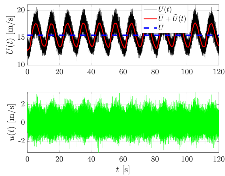
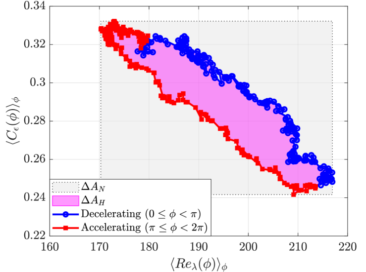
Figure 1: (a) Example of the triple decomposition of an experimental velocity signal into its mean, periodic, and turbulent components. (b) The resulting phase-averaged hysteresis loop in the ($\langle Re_{\lambda}\rangle_{\phi}$, $\langle C_{\epsilon}\rangle_{\phi}$) plane for a representative case, showing the distinct decelerating (blue) and accelerating (red) paths. The shaded area in magenta represents the area of the hysteresis, $\Delta A_{H}$. $\varepsilon$ and the Taylor scale $\lambda$ were estimated using standard spectral techniques [16].

These extensive experimental results are complemented by DNSs, which provide full spatio-temporal data for validation. The incompressible Navier-Stokes equations are solved in a three-dimensional $2\pi L_{0}$-periodic cubic box (with a spatial resolution of $N^{3}=512^{3}$ grid points) with a parallel pseudo-spectral method using the GHOST code [17, 18]. The kinematic viscosity is $\nu_{512}=5\times 10^{-4}\penalty 10000\ L_{0}\overline{U}$. The external forcing is given by a superposition of all modes in the $kL_{0}\in[1,2)$ Fourier shell, generated with random phases. The flow is forced with constant forcing amplitude $A$ until reaching a turbulent steady state. Afterwards, the global amplitude of the forcing is modulated with amplitude $A+\delta A\sin(2\pi t/T)$, integrating the flow for several cycles. Simulations were performed with $\delta A/A=1/4$ and $T=50L_{0}/\overline{U}$, $\delta A/A=1/4$ and $T=25L_{0}/\overline{U}$, and $\delta A/A=1/8$ and $T=50L_{0}/\overline{U}$. Spatial isotropic energy spectra, and the full velocity field ${\bf u}({\bf x},t)$, allow direct computation of all quantities below without assuming Taylor’s hypothesis. As for the HWA, the values of $\varepsilon$ and $\lambda$ were estimated according with standard techniques that are consistent with the HWA calculations [12].

The hysteresis phenomenon introduced in Fig. 1(b) is not an isolated case but a robust feature of the forced turbulent flows investigated. Fig. 2 shows a gallery of phase-averaged hysteresis loops obtained from a wide range of our experimental and numerical configurations. Both the experimental HWA data from different grid geometries and for different external forcing (Fig. 2(a)) and the DNS results at different Reynolds numbers (Fig. 2(b)) consistently exhibit these loops. While the size and shape of the hysteresis varies with the grid and forcing parameters, its existence is a persistent feature.

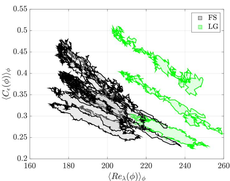
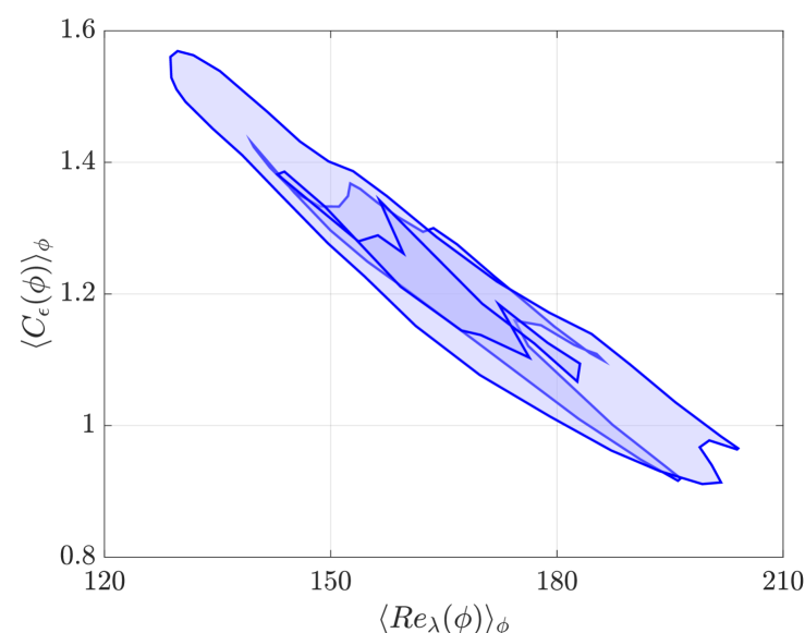
Figure 2: Gallery of phase-averaged hysteresis loops in the ($\langle Re_{\lambda}\rangle_{\phi}$, $\langle C_{\epsilon}\rangle_{\phi}$) plane for various forcing conditions, demonstrating the robustness of the phenomenon in both (a) experiments and (b) simulations.

To move from a qualitative observation to a predictive framework, we now focus on the relationship between the forcing and the resulting hysteresis. By inspecting the unsteady term in Eq. (1), we propose a new dimensionless parameter, $X$, that combines the Strouhal number based on the forcing frequency, $St_{f}=(L/u^{\prime})\cdot f$, where $L$ is the integral length scale and $u^{\prime}$ is the RMS of the velocity fluctuations, and the relative amplitude of the velocity modulation, $|\widetilde{U}|/\overline{U}$. This parameter, $X=St_{f}\cdot(|\widetilde{U}|/\overline{U})$, represents a complete measure of the large-scale unsteadiness imposed on the flow. In experiments, $L$ is calculated, following a standard procedure, integrating the autocorrelation function $R_{u}$ until the first zero crossing [3]. On the other hand, for the DNS it is estimated via the energy spectrum $E(\kappa)$, as $L=\pi/(2u^{\prime 2})\int E(\kappa)/\kappa d\kappa$, where $\kappa$ is the wavenumber in Fourier space. We remark that both formulae are mathematically equivalent.

In particular, we find that hysteresis amplitude and the dimensionless number are correlated. Fig. 3 shows the normalized hysteresis area, $\Delta\langle C_{\epsilon}(\phi)\rangle_{\phi}$, as a function of the dimensionless forcing parameter $X$ for all our experimental and numerical cases. It can be observed that $\Delta\langle C_{\epsilon}(\phi)\rangle_{\phi}$ increases with $X$, with a behavior that depends on the inflow conditions. For instance, in the FS grid case, which corresponds to the configuration with the largest number of data points, a linear relationship between the two parameters is observed. Although only three points are available for the LG grid and the DNS, a similar trend can be identified, albeit with a larger scatter. Despite the relevance of these observations, the estimation of $\Delta\langle C_{\epsilon}(\phi)\rangle_{\phi}$ carries significant uncertainties, as indicated by the nontrivial shapes of the hysteresis cycles shown in Fig. 2.

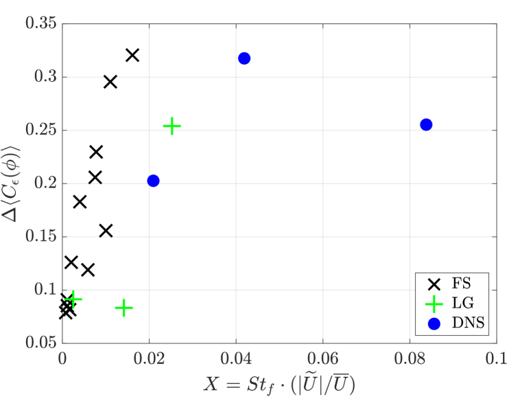
Figure 3: Normalized hysteresis area, $\Delta\langle C_{\epsilon}(\phi)\rangle_{\phi}$, as a function of the dimensionless forcing parameter $X=St_{f}\cdot(|\widetilde{U}|/\overline{U})$. The data includes all experimental (HWA) and numerical (DNS) configurations.

Remarkably, the trends presented in Fig. 3 can be directly linked to the physics of the unsteady energy cascade. Indeed, the hysteresis in the dissipative state can be quantified by the non-zero unsteady term in Eq. (1). We quantify this term using the non-dimensional unsteady function $F(r)$ [10], which is defined as,

$$F(r)\equiv-\frac{3}{\epsilon r^{5}}\int_{0}^{r}s^{4}\frac{\partial}{\partial t}\overline{\delta u^{2}}ds,$$ (2)

and represents the normalized, large-scale unsteadiness of the flow.

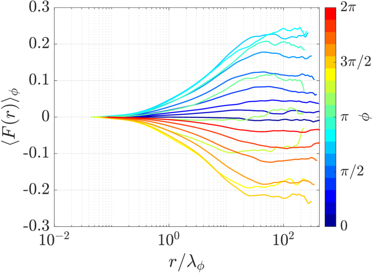
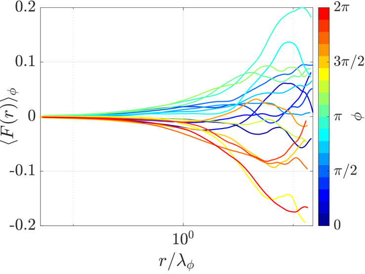
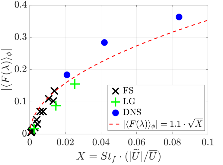
Figure 4: (a) Experimental result of the phase-averaged profiles of the unsteady function, $\langle F(r)\rangle_{\phi}$, versus the non-dimensional lag, $r/\lambda_{\phi}$, for a representative case. (b) DNS result, for a representative case. The curves in (a) and (b) are colored by phase, where phases $\phi\in[0,\pi)$ correspond to the decelerating part of the cycle (cool colors) and $\phi\in[\pi,2\pi)$ to the accelerating part (warm colors). (c) Scaling of the peak-to-peak amplitude of the unsteady function evaluated at the Taylor scale, $|\langle F(\lambda)\rangle_{\phi}|$, with the dimensionless forcing parameter, $X$. The scaling includes all experimental and numerical data.

Fig. 4(a) shows the phase-averaged unsteady function, $\langle F(r)\rangle_{\phi}$, plotted against the non-dimensional lag, $r/\lambda_{\phi}$ (where $\lambda_{\phi}$ is the Taylor microscale of the flow), for a representative experimental case. The function’s shape and magnitude evolve significantly throughout the forcing cycle, confirming that the energy balance is in a constant state of flux. During the decelerating half of the cycle ($\phi\in[0,\pi]$), $\langle F\rangle_{\phi}$ is predominantly positive, indicating a net release of energy from the large scales (i.e., the decay rate exceeds the production rate). Conversely, during the accelerating phase ($\phi\in[\pi,2\pi]$), $\langle F\rangle_{\phi}$ becomes negative, indicating a net storage of energy in the large scales. The amplitude of this oscillation serves as a direct, physical measure of the strength of the unsteadiness within the turbulent cascade. The DNSs present a similar behaviour (Fig. 4(b)). We also note that, given that $\langle F\rangle_{\phi}$ is defined in integral form in Eq. (2), it presents less scatter that the hysteresis cycles reported above.

Fig. 4(c) shows the peak-to-peak amplitude of the unsteady function at the Taylor scale, $|\langle F(\lambda)\rangle_{\phi}|$, against the dimensionless forcing parameter, $X$. Remarkably, a good collapse is observed for all all experimental and numerical data. Moreover, the relation $F(\lambda)\propto\sqrt{X}$ fits the data trend. This proves that our macroscopic forcing parameter is not only associated with the hysteresis area, but is a direct proxy for the magnitude of the underlying physical cause (the unsteady term in the KH equation). In consequence, the balance within the inertial range between the dissipative and the inter-scale energy transfer terms from Eq. (1) is altered by the effect of the unsteady term. This term can be both positive and negative during the cycle, producing a measurable effect in the dissipation constant $C_{\varepsilon}$. Moreover, when a solenoidal forcing is considered, as $F$ is defined positive for decelerating flows, the KH equation also justifies that the upper branch of the hysteresis cycle corresponds to such regime of the flow. This provides, therefore, a quantitative explanation of the observations of Fig. 2, relating the intensity of the hysteresis cycle with the unsteady flow nature.

In summary, we have established a framework for the onset of hysteresis in the turbulent energy cascade. Combining HWA experiments and DNS of periodically forced turbulence, we identified a universal scaling law linking the hysteresis magnitude (measured by the normalized area of the $(\langle Re_{\lambda}\rangle_{\phi},\langle C_{\epsilon}\rangle_{\phi})$ loop) to a single dimensionless forcing parameter, $X$. This law is physically grounded in the energy balance of the flow, as $X$ scales with the square of the unsteady term in the KH equation. Our findings thus reveal that hysteresis is a macroscopic signature of the time-dependent energy transfer within the cascade, providing a simple predictive link between large-scale forcing and instantaneous turbulent dissipation.

The implications of this finding are significant. It provides a simple predictive tool for estimating the degree to which a turbulent flow will depart from a quasi-steady state based on the characteristics of its unsteady boundary conditions. The ability to predict the magnitude of the cascade’s hysteresis from simple, large-scale parameters is a crucial step towards developing more advanced models for a wide range of real-world out-of-equilibrium systems. This includes industrial processes that involve pulsating jets or mixers, and natural phenomena such as atmospheric turbulence interacting with gusts or the transport of pollutants and aerosols in unsteady winds, where understanding the unsteady dynamics is of paramount importance [1, 12]. More work needs to be devoted to the generalization of our findings to other flows and its validation for a broader range of non-dimensional forcing parameters $X$. Furthermore, the existence of a time lag between the Reynolds number and dissipation should be addressed in future works.