Distributionally Robust Dynamic Structural Estimation: Serial Dependence and Sensitivity Analysis

Distributional assumptions that discipline serially correlated latent variables play a central role in dynamic structural models. We propose a framework to quantify the sensitivity of scalar parameters of interest (e.g., welfare, elasticity) to such distributional assumptions. We derive bounds on the scalar parameter by perturbing a reference distribution, while imposing a stationarity condition for time-homogeneous models or a Markovian condition for time-inhomogeneous models. The bounds are the solutions to optimization problems, for which we derive a computationally tractable dual formulation. We establish consistency, convergence rate, and asymptotic distribution for the estimator of the bounds. We demonstrate the approach with two applications: an infinite-horizon dynamic demand model for new cars in the United Kingdom, Germany, and France, and a finite-horizon dynamic labor supply model for taxi drivers in New York City. In the car application, perturbed price elasticities deviate by at most 15.24% from the reference elasticities, while perturbed estimates of consumer surplus from an additional $3,000 electric vehicle subsidy vary by up to 102.75%. In the labor supply application, the perturbed Frisch labor supply elasticity deviates by at most 76.83% for weekday drivers and 42.84% for weekend drivers.

Keywords: Serial dependence, Sensitivity analysis, Dynamic structural models, Robustness, Misspecification

JEL Codes: C14, C18, C51, C61

1 Introduction

Dynamic structural models are useful tools for counterfactual policy analysis in various fields of economics. The correlation structure of latent variables is a key feature of these models, as it captures the persistence of unobserved factors that affect agents’ decisions over time. Examples of potentially serially correlated latent variables include: product characteristics in demand estimation (Nair, (2007); Schiraldi, (2011); Gowrisankaran and Rysman, (2012)), search costs in consumer search (Koulayev, (2014)), firm productivity in trade (Piveteau, (2021)), patent profitability in optimal stopping (Pakes, (1984)), quality in technology adoption (De Groote and Verboven, (2019)), health shocks in insurance (Fang and Kung, (2021)), and beliefs about ability in labor economics (Miller, (1984); Arcidiacono et al., (2025)).

Distributional assumptions about the serial dependence of latent variables play a central role in the estimation and counterfactual analysis of dynamic structural models. These assumptions capture agents’ uncertainty about the future, such as a consumer’s uncertainty about future product characteristics in demand estimation. The misspecification of these assumptions can lead to biased estimates of future continuation value, which in turn bias counterfactual predictions (e.g., welfare and elasticity). However, the direction and magnitude of this bias are unclear, because the models are dynamic and nonlinear. This raises the need for sensitivity analysis of empirical results to these distributional assumptions.

In this paper, we propose a framework to quantify this sensitivity by perturbing a reference distribution to compute bounds on a scalar parameter of interest. The scalar parameter (e.g., welfare and elasticity) is a function of model primitives, such as model parameters, the distribution of latent variables, and the value function in dynamic structural models. In our proposed framework, the bounds on this scalar parameter are the solutions to constrained optimization problems whose feasible region (identified set) is defined by moment conditions for estimation, structural constraints (e.g., the Bellman equation), and the perturbation set around the reference distribution. The distribution that attains the bound is called the worst-case distribution.

A central challenge is to define the perturbation set in a way that simplifies computation while maintaining key structural features of the distribution of latent variables. For time-homogeneous models, the structural feature is the stationarity condition, i.e., the perturbed transition distribution must be stationary. For finite-horizon, time-inhomogeneous models, the perturbed trajectory of latent variables must be Markovian. In addition, the terminal distribution is fixed becuase it can be nonparametrically point identified (Lewbel, (2000); Matzkin, (2007)). Because the stationarity and Markov conditions are functional constraints imposed directly on the distribution being optimized, they are computationally difficult to impose. We contribute to the sensitivity analysis literature (e.g., Christensen and Connault, (2023)) by providing a computationally tractable framework to deal with these constraints.

There are further practical challenges. First, the properties (e.g., closed-form, smoothness) of the worst-case distribution are typically unclear, complicating the choice of approximation methods. Second, the expectations that define the scalar parameter, the model-implied moments, and the structural constraints are all calculated with respect to the perturbed distribution. Because this distribution is itself an optimization variable that changes during the optimization, the numerical integration can be difficult to implement. Third, the value function in dynamic structural models is infinite-dimensional due to the serial dependence of latent variables, which complicates the optimization problem further.

To address these challenges, we define the perturbation set as a Kullback-Leibler (KL) divergence ball around the reference distribution. The KL radius controls the size of the perturbation set. Then, we employ the Optimal Transport (OT) framework to impose constraints on the distribution of latent variables. These constraints, combined with the KL divergence constraint, form a computationally tractable entropic optimal transport (EOT) problem. For the time-homogeneous case, the reference distribution is a joint distribution of current and future latent variables. The stationarity condition requires that the marginal distributions of current and future latent variables of the perturbed joint distribution are the same, which can be imposed using OT. This marginal constraint, when combined with the KL divergence penalty from the problem’s Lagrangian, forms an EOT problem. For the time-inhomogeneous case, the perturbed trajectory must be Markovian, and the terminal distribution is fixed. We show how to formulate this as an EOT problem.

The EOT problem can be solved using its dual formulation, which has three key advantages over the primal formulation. First, it provides a closed-form expression for the worst-case distribution and characterizes its smoothness. During our proposed optimization algorithm, this closed-form expression is used to update the value function in dynamic structural models. Second, the Sinkhorn algorithm (Sinkhorn and Knopp, (1967); Cuturi, (2013)) allows us to solve the EOT problem and compute the worst-case distribution efficiently. Finally, because the expectations in the dual problem are taken with respect to the reference distribution, an appropriate numerical integration method can be chosen in advance.

Then, we propose three complementary sensitivity measures to interpret the results. First, the global sensitivity approach computes the largest deviation from the reference value. It progressively increases the KL radius until the bounds flatten. We show that it provides a tractable approximation to the nonparametric bounds on the scalar parameter when the KL divergence constraint is removed. Second, the local sensitivity approach analyzes the effect of small perturbations. It computes the right derivatives of the bounds with respect to the KL radius at zero, which is our local sensitivity measure. Finally, the robustness metric approach, inspired by Spini, (2024), computes the smallest deviation from the reference distribution required to produce sensitive results. It is the smallest KL divergence from the reference distribution required for the scalar parameter’s value to fall below a user-specified threshold (e.g., 5% below the reference value). In addition to our three sensitivity measures, we can also estimate an alternative model and set the radius as the KL divergence between the alternative and reference models.

For estimation and inference, we propose an estimator for the bound, establishing its consistency and convergence rate. To this end, we first establish the consistency and convergence rate of the estimator of the identified set, following Chernozhukov et al., (2007). We then derive the asymptotic distribution of the plug-in estimator by proving the Hadamard directional differentiability of the bound, building on the work of Fang and Santos, (2019).

We apply our framework to an infinite-horizon dynamic demand model for new cars in the UK, Germany, and France. We consider the sensitivity of the price elasticity and consumer surplus from an additional $3,000 electric vehicle subsidy. In the model, the indirect utility of purchasing is a latent variable due to unobserved product characteristics, and its transition is typically modeled as an AR(1) process (e.g., Schiraldi, (2011); Gowrisankaran and Rysman, (2012)). For the price elasticity, we find that the French market is the least sensitive to the distributional assumption (at most 6.20% deviation from the reference elasticity), while the German market is the most sensitive (at most 15.24% deviation). We also find that this sensitivity is relatively stable over time for all three markets. For the consumer surplus, the German market is also the most sensitive (at most 102.75% deviation from the reference consumer surplus), while the UK and French markets are less sensitive (at most 25.17% and 24.73% deviation, respectively). More importantly, the results are still economically meaningful even under the worst-case distribution, with the consumer surplus remaining at least $309 million for the German market, $1,243 million for the French market, and $2,584 million for the UK market.

We also apply our framework to a finite-horizon dynamic labor supply model for taxi drivers in New York City. We consider the sensitivity of the elasticity of stopping work and the Frisch elasticity of labor supply. In the model, the market-level supply shock is a latent variable. The reference distribution is also modeled as an AR(1) process. For the elasticity of stopping work, we find that weekday drivers’ elasticity is more sensitive in the morning, while weekend drivers’ elasticity is more sensitive in the afternoon. For the Frisch elasticity, both weekday and weekend drivers’ elasticities are sensitive to the distributional assumption, with at most 76.83% and 42.84% deviation from the reference elasticity, respectively.

1.1 Related Literature

Identification and estimation. Many papers have focused on identification in a range of dynamic structural models including finite mixture models (Kasahara and Shimotsu, (2009); Luo et al., (2022); Higgins and Jochmans, (2023)), unobservable Markov processes (Hu and Shum, (2012)), and counterfactual conditional choice probabilities in dynamic binary choice models (Norets and Tang, (2014)). Berry and Compiani, (2023) uses the generalized instrumental variable approach for unobserved state variables in dynamic discrete choice (DDC) models. In fixed effects DDC models, Aguirregabiria et al., (2021) considers identification of structural parameters using sufficient statistics, while Aguirregabiria and Carro, (2024) studies identification of average marginal effects. Hwang, (2024) employs proxy variables for the latent variables. Kalouptsidi et al., 2021c proposes the Euler Equations in Conditional Choice Probabilities (ECCP) estimator. By leveraging finite-dependence properties and cross-sectional data, it identifies structural parameters in the presence of serially correlated market-level unobserved variables without distributional assumptions. Arcidiacono and Miller, (2011) adapts the Expectation-Maximization algorithm to estimate DDC models with discrete latent types. Norets, (2009) extends the Bayesian estimation of DDC models by Imai et al., (2009) to allow for serially correlated latent variables, while Blevins, (2016) proposes a sequential Monte Carlo method. Chiong et al., (2016) shows identification in DDC models is an optimal transport problem under serial independence of utility shocks. In addition, Chen et al., (2011), Schennach, (2014), and Fan et al., (2023, 2025) consider inference of finite-dimensional parameters in the presence of an infinite-dimensional parameter, namely the distribution of latent variables.

Our framework contributes to this literature in three ways. First, we focus on a scalar parameter (outcome of interest) directly instead of the identified set of model primitives. Second, to analyze sensitivity, we consider a perturbation set around the reference distribution rather than the set of all distributions. Third, we complement identification strategies that do not rely on distributional assumptions. In the labor supply application, we use the ECCP estimator by Kalouptsidi et al., 2021c to point identify the utility parameters, and then conduct sensitivity analysis of the labor supply elasticity to the distributional assumption about the market-level supply shock.

Sensitivity analysis and robustness. In DDC models, Kalouptsidi et al., 2021a ; Kalouptsidi et al., 2021b relax common normalization on the utility function. Bugni and Ura, (2019) considers the local misspecification of the transition density of observable variables, assuming the transition density is correctly specified in the limit (as the sample size goes to infinity) in DDC models. Andrews et al., (2017) considers a setting in which the moments are locally misspecified under the reference distribution. Subsequent work, Armstrong and Kolesár, (2021), constructs near-optimal confidence intervals in such models. In contrast, we perturb the reference distribution subject to the moment conditions. Bonhomme and Weidner, (2022) perturbs the reference model and assumes the size of the perturbation shrinks to zero as the sample size goes to infinity. Chen et al., (2024) relaxes the rational expectation assumption. Gu and Russell, (2024) considers the identification of scalar counterfactual parameters using optimal transport. Spini, (2024) studies the robustness of policy effects to changes in the distribution of covariates. Armstrong, (2025) provides a selective review of misspecification in econometrics. Most closely related is Christensen and Connault, (2023), who conducts sensitivity analysis with respect to parametric assumptions about the distribution of latent variables in structural models. However, they focus on relaxing the marginal distribution assumption while maintaining serial independence.

We contribute to this literature in three ways. First, our focus on serial dependence complements analyzes of misspecification in the marginal distribution assumption (e.g., Christensen and Connault, (2023)). Second, the size of our perturbation set is fixed and does not shrink with the sample size. Third, we provide a computationally tractable dual formulation for the optimization problem. While prior work (Schennach, (2014); Gu and Russell, (2024); Christensen and Connault, (2023)) uses duality to convert the infinite-dimensional problem to a finite-dimensional one, our dual problem is still infinite-dimensional. This is because the stationarity condition for time-homogeneous models and fixed terminal distribution for time-inhomogeneous models are infinite-dimensional, and serial dependence leads to an infinite-dimensional value function in dynamic structural models. However, by leveraging EOT duality, we provide a tractable implementation and demonstrate our approach through two empirical applications.

Distributionally robust optimization (DRO). The literature on DRO (Kuhn et al., (2019); Rahimian and Mehrotra, (2019); Blanchet et al., (2022); Gao and Kleywegt, (2023); Wang et al., (2021)) usually studies the uncertainty due to limited observability of data, noisy measurements, or estimation errors.

Our work is distinct in that we study the misspecification due to assumptions about the serial dependence of latent variables—a problem of model specification rather than data limitation. In addition, because our framework can be treated as a moment-constrained DRO problem, we employ the minimax theorem (see Fan, (1953) and Ricceri and Simons, (1998), Theorem 1.3) to exchange the order of the supremum over Lagrangian multipliers (for the moment conditions and structural constraints) and the infimum over distributions in the perturbation set. This exchange allows a direct application of duality results from the DRO literature.

Applied work. Building on the seminal work on the estimation of DDC models (Rust, (1987); Hotz and Miller, (1993); Aguirregabiria and Mira, (2002, 2007); Pesendorfer and Schmidt-Dengler, (2008); Arcidiacono and Miller, (2011)), most applied work assumes the serial independence of utility shocks. In the presence of serially correlated latent variables, parametric models are often used, as seen in the works of Schiraldi, (2011); Gowrisankaran and Rysman, (2012); Blevins et al., (2018); Piveteau, (2021) and others mentioned in the introduction.

We contribute to this literature by developing a computationally tractable framework for sensitivity analysis of scalar parameters of interest to these distributional assumptions. We also demonstrate our framework through two empirical applications: an infinite-horizon dynamic demand model, and a finite-horizon dynamic labor supply model.

Outline: Sections 2 and 3 present our framework for time-homogeneous and time-inhomogeneous models. Section 4 establishes the large sample properties of our estimator. Section 5 introduces three sensitivity measures. Section 6 discusses practical implementation. Sections 7 and 8 present two empirical applications. Section 9 concludes. Appendix A presents two additional examples. All proofs are in Appendix B.

Notation: Let $U\in\mathcal{U}\subseteq\mathbb{R}^{d}$ be a vector of latent variables with support $\mathcal{U}$ where $\mathcal{U}$ is assumed to be Polish. Let $\mathcal{P}(\mathcal{U})$ be the space of Borel probability measures on $\mathcal{U}$ and $\mathcal{B}(\mathcal{U})$ be the Borel $\sigma$-algebra on $\mathcal{U}$. In this paper, all measures are assumed to be absolutely continuous with respect to the Lebesgue measure. Denote by $\mathbb{E}_{F}\left[\cdot\right]$, $\mathbb{E}_{x}\left[\cdot\right]$ the expectations with respect to $F\in\mathcal{P}(\mathcal{U})$ and the probability distribution of the random variable $x$, respectively. For variables in a stationary dynamic context, a prime (e.g., $x^{\prime}$) denotes the variable’s value in the next period. Let $F_{1},F_{2}\in\mathcal{P}(\mathcal{U})$, we write $F_{1}\ll F_{2}$ if $F_{1}$ is absolutely continuous with respect to $F_{2}$, and $F_{1}\otimes F_{2}$ as the product measure. For a finite-dimensional vector, denote by $\|\cdot\|_{p}$ the $p$-norm. Denote by $L^{p}(F)$ the space of functions for which $\int|f|^{p}dF<\infty$. For a set $\mathcal{A}$, denote by $\text{int}(\mathcal{A})$ its interior. Denote by $\mathbb{R}_{+}$ the set of non-negative real numbers, and $\mathbb{N}$ the set of natural numbers. Finally, let $\mathcal{J}:=\left\{1,\cdots,J\right\}$.

2 Methodology for Time-Homogenous Models

This section develops our methodology for time-homogeneous models. We first define the perturbation set in Section 2.1, and present two examples in Section 2.2. Then, we present a general framework that nests the examples, and derive its duality in Section 2.3. Finally, Section 2.4 discusses how to perturb the stationary distribution.

2.1 Definition of Perturbation Set

We partition a vector of latent variables $U\in\mathcal{U}\subseteq\mathbb{R}^{d}$ into $2\leq k\leq d$ subvectors, i.e., $U=(U_{1},\cdots,U_{k})$. Each subvector $U_{i}\in\mathcal{U}_{i}\subseteq\mathbb{R}^{d_{i}}$ has a marginal distribution $\nu_{i}\in\mathcal{P}(\mathcal{U}_{i})$ for $i=1,\cdots,k$. Let $F_{0}$ denote the reference distribution for $U$. The perturbation set around this reference distribution is defined as:

$$\mathcal{F}:=\left\{F\in\mathcal{P}(\mathcal{U})\mid F\in\Pi(\nu_{1},\cdots,\nu_{k}),D_{KL}(F\|F_{0})\leq\delta\right\}$$

where $\Pi(\nu_{1},\cdots,\nu_{k})$ is the set of joint distributions on $\mathcal{U}$ with marginals $\{\nu_{i}\}_{i=1}^{k}$, and $\delta\geq 0$ measures the “size” of the perturbation set, defined by the Kullback-Leibler (KL) divergence:

$$D_{KL}(F\|F_{0}):=\begin{cases}\int\log\left(\frac{dF(U)}{dF_{0}(U)}\right)dF(U)&\text{if }F\ll F_{0}\\ +\infty&\text{otherwise}\end{cases}$$

In time-homogeneous models, the marginal constraints are used to impose the stationarity. Consider an unobserved stationary first-order Markov process $\{\xi_{t}\}_{t\in\mathbb{Z}}$ with state space $\Xi\subseteq\mathbb{R}^{d_{\xi}}$. The process is stationary with respect to $\nu_{0}\in\mathcal{P}(\Xi)$ if $\int F_{0}(d\xi^{\prime}|\xi)\nu_{0}(d\xi)=\nu_{0}(d\xi^{\prime})$ for all $\xi^{\prime}\in\Xi$, where $F_{0}(d\xi^{\prime}|\xi)$ is the reference transition kernel (e.g., conditional Gaussian distribution for an AR(1) process). This is equivalent to requiring that the marginal distributions of the joint distribution $dF_{0}(\xi,\xi^{\prime}):=F_{0}(d\xi^{\prime}|\xi)\nu_{0}(d\xi)$ are both $\nu_{0}$, i.e., $F_{0}\in\Pi(\nu_{0},\nu_{0})$. Moreover, for any $F\in\Pi(\nu_{0},\nu_{0})$, its conditional density $F(d\xi^{\prime}|\xi)$ preserves $\nu_{0}$ as a stationary distribution. For this example, let $U:=(\xi,\xi^{\prime})$. Then, the perturbation set is:

$$\mathcal{F}:=\{F\in\mathcal{P}(\mathcal{U})\mid F\in\underbrace{\Pi(\nu_{0},\nu_{0})}_{\text{Stationarity}},\underbrace{D_{KL}(F\|F_{0})\leq\delta}_{\text{Perturbation}}\}$$

This definition allows us to perturb the transition kernel of the Markov process while keeping its stationary distribution unchanged. It can introduce non-linear dynamics into the latent variable process. For example, if the reference model is an AR(1) process, the perturbation set includes any nonlinear first-order Markov process with the same stationary distribution as the AR(1) process. Section 2.4 discusses how to perturb the stationary distribution. In this case, we replace the condition $F\in\Pi(\nu_{0},\nu_{0})$ with $F\in\Pi(\nu,\nu)$, where $\nu$ is the perturbed stationary distribution that is in a neighborhood of $\nu_{0}$.

2.2 Examples

This section presents two examples of single-agent DDC models. We focus on a parametric model for latent variables in both infinite and finite-horizon DDC models. Appendix A presents two additional examples: (i) serial independence of utility shocks in DDC models (ii) serial independence of consumption shocks in dynamic discrete-continuous choice models. Our framework seeks to find the lower bound on a scalar parameter of interest by solving a constrained optimization problem over the perturbation set that is subject to the structural constraints (e.g., Bellman equation) and moment conditions.

Example 1 (Infinite Horizon Dynamic Discrete Choice Models with Serially Correlated Latent Variables).

This example considers a parametric model for serially correlated latent variables in a single-agent DDC model as in Rust, (1994). Let $\xi\in\Xi$ be the exogenously evolving latent variable. Agents solve the smoothed Bellman equation for the conditional value function $v\in\mathcal{V}$ where $\mathcal{V}$ is a function class (e.g., square integrable functions, the Hölder class, etc.): for $\forall\ (x,\xi,j)\in\mathcal{X}\times\Xi\times\mathcal{J}$, it holds that

$$v_{j}(x,\xi)=\pi_{j}(x,\xi;\theta)+\beta\mathbb{E}_{\xi^{\prime}|\xi}\mathbb{E}_{x^{\prime}|x,j}\left[\log\left(\sum_{j^{\prime}\in\mathcal{J}}\exp(v_{j^{\prime}}(x^{\prime},\xi^{\prime}))\right)\right]+\beta\gamma$$ (1)

where $x\in\mathcal{X}$ is the observable state variable, $\beta\in(0,1)$ is the discount factor, $\gamma$ is the Euler constant, and $\pi_{j}(x,\xi;\theta)$ is the period utility of choosing action $j\in\mathcal{J}$ parameterized by $\theta\in\Theta$. The model-implied Conditional Choice Probability (CCP) is:

$$p(j|x,\xi)=\frac{\exp\left(v_{j}(x,\xi)\right)}{\sum_{j^{\prime}\in\mathcal{J}}\exp\left(v_{j^{\prime}}(x,\xi)\right)}$$

Let $U:=(\xi,\xi^{\prime})$ be a vector of current and future latent variables. An AR(1) process is often used to model the transition of $\xi$. Therefore, the reference distribution is $dF_{\theta_{f}}(U):=F_{\theta_{f}}(d\xi^{\prime}|\xi)\nu_{\theta_{f}}(d\xi)$ where $F_{\theta_{f}}(d\xi^{\prime}|\xi)$ is the conditional distribution parameterized by $\theta_{f}\in\Theta_{f}$ (e.g., the parameters of the AR(1) process), and $\nu_{\theta_{f}}$ is its stationary distribution. The perturbation set for a given $\theta_{f}$ is defined as:

$$\mathcal{F}_{\theta_{f}}:=\left\{F\in\mathcal{P}(\mathcal{U})\mid F\in\Pi(\nu_{\theta_{f}},\nu_{\theta_{f}}),D_{KL}(F\|F_{\theta_{f}})\leq\delta\right\}$$

Suppose the scalar parameter of interest is the average elasticity of action $j$ with respect to variable $x_{l}$, defined as:

$$\mathbb{E}_{\nu_{\theta_{f}}}\mathbb{E}_{x}\left[\frac{\partial p(j|x,\xi)}{\partial x_{l}}\frac{x_{l}}{P_{0}(j|x)}\right]$$

where $P_{0}(j|x)$ is the population CCP, and the expectation is taken with respect to the joint distribution $F\in\mathcal{F}_{\theta_{f}}$ and the distribution of $x$.

We convert the smoothed Bellman equation (1) into an unconditional moment restriction that depends on the joint distribution $F$. We assume there exists a class of Lagrange multiplier functions $\mathcal{G}$ such that $v$ solves the Bellman equation (1) if and only if:

$$\sup_{g\in\mathcal{G}}\mathbb{E}_{F}\mathbb{E}_{x,j,x^{\prime}}\left[g_{j}(x,\xi)\left(v_{j}(x,\xi)-\pi_{j}(x,\xi;\theta)-\beta\log\left(\sum_{j^{\prime}\in\mathcal{J}}\exp(v_{j^{\prime}}(x^{\prime},\xi^{\prime}))\right)-\beta\gamma\right)\right]=0$$

where the inner expectation is taken with respect to the stationary distribution of $x$, the population CCPs, and the conditional distribution of $x^{\prime}$ given $(x,j)$. Let $g:=(g_{j})_{j\in\mathcal{J}}$. Then, we rewrite the structural constraints as:

$$\sup_{g\in\mathcal{G}}\mathbb{E}_{F}\left[\psi(U;\theta,v,g)\right]=0$$

We consider the following moment conditions for estimation:

$$\mathbb{E}_{\nu_{\theta_{f}}}\left[p(j|x,\xi)\right]=P_{0}(j|x)\quad\forall\ (j,x)\in\mathcal{J}\times\mathcal{X}$$

We assume $\mathcal{X}$ has discrete support, and rewrite the moment conditions as:

$$\mathbb{E}_{F}\left[m(U;v)\right]=P_{0}$$

where $m(U;v)$ stacks the model-implied CCPs, and $P_{0}$ stacks the population CCPs.

Then, the lower bound on the elasticity is given by:

$$\inf_{\theta_{f}\in\Theta_{f}}\inf_{(\theta,v,F)\in\Theta\times\mathcal{V}\times\mathcal{F}_{\theta_{f}}}\ \mathbb{E}_{\nu_{\theta_{f}}}\mathbb{E}_{x}\left[\frac{\partial p(j|x,\xi)}{\partial x_{l}}\frac{x_{l}}{P_{0}(j|x)}\right]$$

s.t. $$\mathbb{E}_{F}\left[m(U;v)\right]=P_{0}$$

$$\sup_{g\in\mathcal{G}}\mathbb{E}_{F}\left[\psi(U;\theta,v,g)\right]=0$$

In the next section, we will discuss the implementation for a fixed $\theta_{f}$. The overall lower bound requires an additional optimization over $\theta_{f}\in\Theta_{f}$. In practice, we can discretize the estimated AR(1) process, and scale the grid points according to the candidate $\theta_{f}$ during the optimization. Then, the optimization over $\theta_{f}$ can be implemented using the algorithm proposed in Section 6.2.

Example 2 (Finite Horizon Dynamic Discrete Choice Models).

This example considers a finite-horizon DDC model where the latent variable $\xi\in\Xi$ follows a first-order stationary Markov process. The conditional value function $v_{t}\in\mathcal{V}$ at time period $t\leq T<+\infty$ solves the smoothed Bellman equation: for $\forall\ (x_{t},\xi_{t},j)\in\mathcal{X}\times\Xi\times\mathcal{J}$,

$$v_{jt}(x_{t},\xi_{t})=\pi_{j}(x_{t},\xi_{t};\theta)+\beta\mathbb{E}_{\xi_{t+1}|\xi_{t}}\mathbb{E}_{x_{t+1}|x_{t},j}\left[\log\left(\sum_{j^{\prime}\in\mathcal{J}}\exp(v_{jt+1}(x_{t+1},\xi_{t+1}))\right)\right]+\beta\gamma$$ (2)

where $x\in\mathcal{X}$ is the observable state variable, $\beta\in(0,1)$ is the discount factor, $\gamma$ is the Euler constant, $\pi_{j}(x,\xi;\theta)$ is the period utility parameterized by $\theta\in\Theta$, and $v_{jT}(x_{T},\xi_{T})=\pi_{j}(x_{T},\xi_{T};\theta)$. The model-implied CCP is:

$$p_{t}(j|x,\xi)=\frac{\exp\left(v_{jt}(x,\xi)\right)}{\sum_{j^{\prime}\in\mathcal{J}}\exp\left(v_{j^{\prime}t}(x,\xi)\right)}$$

Let $U:=(\xi,\xi^{\prime})$ be a vector of current and future latent variables. In practice, we may set the reference distribution as the estimated distribution from a parametric model, such as an AR(1) process. The reference distribution $F_{0}$ is the product of the conditional distribution and its stationary distribution, $\nu_{0}$. The perturbation set is defined as:

$$\mathcal{F}:=\left\{F\in\mathcal{P}(\mathcal{U})\mid F\in\Pi(\nu_{0},\nu_{0}),D_{KL}(F\|F_{0})\leq\delta\right\}$$

Suppose the scalar parameter of interest is the consumer surplus derived from the choice set $\mathcal{J}$ at period $t$:

$$\mathbb{E}_{\nu_{0}}\mathbb{E}_{x_{t}}\left[\frac{1}{\alpha}\log\left(\sum_{j\in\mathcal{J}}\exp(v_{jt}(x_{t},\xi_{t}))\right)\right]$$

where we assume $\pi_{j}(x_{t},\xi_{t};\theta)$ is linear in price and $\alpha$ is the price coefficient.

We convert the smoothed Bellman equation (2) into restrictions that depend on the joint distribution $F\in\mathcal{F}$. We assume there exists a class of Lagrange multiplier functions $\mathcal{G}$ such that for each $t\leq T-1$, $v_{t}$ solves (2) if and only if:

$$\sup_{g_{t}\in\mathcal{G}}\mathbb{E}_{F}\mathbb{E}_{x_{t},j_{t},x_{t+1}}\Big[g_{jt}(x_{t},\xi_{t})$$

$$\qquad\times\Big(v_{jt}(x_{t},\xi_{t})-\pi_{j_{t}}(x_{t},\xi_{t};\theta)-\beta\log\left(\sum_{j^{\prime}\in\mathcal{J}}\exp(v_{j^{\prime}t+1}(x_{t+1},\xi_{t+1}))\right)-\beta\gamma\Big)\Big]=0$$

where $(\xi_{t},\xi_{t+1})\sim F$, $(x_{t},j_{t})$ is distributed according to the observed data at time $t$, and $x_{t+1}$ follows the conditional distribution given $(x_{t},j_{t})$. Let $g:=(g_{jt})_{j\in\mathcal{J},t\leq T-1}$ and $v:=(v_{jt})_{j\in\mathcal{J},t\leq T-1}$. Then, we rewrite the structural constraints as:

$$\sup_{g\in\mathcal{G}}\mathbb{E}_{F}\left[\psi(U;\theta,v,g)\right]=0$$

where $\psi$ is the sum of the objective functions in the above equation for each $t\leq T-1$.

We consider the following moment conditions for estimation: for each $t\leq T$,

$$\mathbb{E}_{\nu_{0}}\left[p_{t}(j|x_{t},\xi)\right]=P_{0t}(j|x_{t})\quad\forall\ (j,x_{t})\in\mathcal{J}\times\mathcal{X}$$

where $P_{0t}(j|x_{t})$ is the population CCP at period $t$. We assume $\mathcal{X}$ has discrete support, and rewrite the moment conditions as:

$$\mathbb{E}_{F}\left[m(U;v)\right]=P_{0}$$

where $m(U;v)$ and $P_{0}$ stack the model-implied and population CCPs for all $t\leq T$.

Then, the lower bound on consumer surplus at period $t$ is given by:

$$\inf_{(\theta,v,F)\in\Theta\times\mathcal{V}\times\mathcal{F}} \mathbb{E}_{\nu_{0}}\mathbb{E}_{x_{t}}\left[\frac{1}{\alpha}\log\left(\sum_{j\in\mathcal{J}}\exp(v_{jt}(x_{t},\xi_{t}))\right)\right]$$

$$\text{s.t.}\quad\mathbb{E}_{F}\left[m(U;v)\right]=P_{0}$$

$$\phantom{\text{s.t.}\quad}\sup_{g\in\mathcal{G}}\mathbb{E}_{F}\left[\psi(U;\theta,v,g)\right]=0$$

2.3 Framework and Duality

We now present a general framework that nests the above examples. In general, the model is not point-identified when $\mathcal{F}$ is not a singleton. Therefore, we propose to compute upper and lower bounds on the outcome of interest. Let the scalar parameter of interest, $s:\mathcal{U}\times\Theta\times\mathcal{V}\rightarrow\mathbb{R}$, be a function of the latent variable $U$, and the model primitives $(\theta,v)\in\Theta\times\mathcal{V}$. The lower bound is the solution to the following optimization problem:

$$\kappa(\delta,P):= \inf_{(\theta,v,F)\in\Theta\times\mathcal{V}\times\mathcal{F}}\mathbb{E}_{F}\left[s(U;\theta,v)\right]$$

$$\text{s.t.}\quad\mathbb{E}_{F}\left[m(U;\theta,v)\right]=P$$ ( Primal)

$$\phantom{\text{s.t.}\quad}\sup_{g\in\mathcal{G}}\mathbb{E}_{F}\left[\psi(U;\theta,v,g)\right]=0$$

where $\mathcal{F}:=\{F\in\mathcal{P}(\mathcal{U})\mid F\in\Pi(\nu_{1},\cdots,\nu_{k}),D_{KL}(F\|F_{0})\leq\delta\}$.

The first constraint is a moment condition where the moment function $m:\mathcal{U}\times\Theta\times\mathcal{V}\rightarrow\mathbb{R}^{d_{P}}$ is finite-dimensional as we assume the observable variable $X\in\mathcal{X}$ has discrete support and stack the moment functions for each $x\in\mathcal{X}$. The second constraint is a structural constraint defined by $\psi:\mathcal{U}\times\Theta\times\mathcal{V}\times\mathcal{G}\rightarrow\mathbb{R}$ that is linear in the Lagrange multiplier function $g\in\mathcal{G}$ for a given $(\theta,v)$. Finally, $v\in\mathcal{V}$ is the solution to the structural constraint.

Remark 1.

1. The upper bound can be obtained by replacing $s(U;\theta,v)$ with $-s(U;\theta,v)$.

2. The moment condition can contain restrictions linear in $F$, e.g., covariance restrictions.

3. If some model primitives (e.g., a subvector of $\theta$) are point-identified, they are treated as fixed values rather than optimized over.

4. The framework can also be applied to models without structural constraints, such as static and panel discrete choice models.

The Primal problem can be intractable due to the optimization over $\mathcal{F}$. First, the properties (e.g., closed-form and smoothness) of the optimal $F^{*}$ are typically unknown, complicating the choice of approximation methods. Second, the marginal distribution conditions are functional constraints imposed directly on the distribution being optimized, which are computationally difficult to impose. Third, expectations are taken with respect to the perturbed distribution, making numerical integration difficult.

To overcome these issues, we derive the Dual problem corresponding to the Primal. The Dual provides the closed-form of the optimal $F^{*}$, and characterizes its smoothness. Moreover, in the dual, the expectation is taken with respect to the reference distribution $F_{0}$. Section 6.2 proposes a computationally tractable algorithm that utilizes the optimal $F^{*}$. To motivate the duality, consider the Lagrangian of the Primal:

$$\kappa(\delta,P)=\inf_{\begin{subarray}{c}(\theta,v)\in\Theta\times\mathcal{V}\\ F\in\Pi(\nu_{1},\ldots,\nu_{k})\end{subarray}}\sup_{\begin{subarray}{c}\lambda\in\mathbb{R}^{d_{P}}\\ \lambda_{KL}\geq 0,g\in\mathcal{G}\end{subarray}}\mathbb{E}_{F}\left[c(U;\theta,v,g,\lambda)\right]+\lambda_{KL}(D_{KL}(F\|F_{0})-\delta)-\lambda^{T}P$$ (3)

where $c(U;\theta,v,g,\lambda):=s(U;\theta,v)+\lambda^{T}m(U;\theta,v)+\psi(U;\theta,v,g)$, $\lambda\in\mathbb{R}^{d_{P}}$ is the Lagrange multiplier for the moment condition and $\lambda_{KL}$ is the Lagrange multiplier for the KL divergence constraint. For given $(\theta,v)$, under regularity conditions, we can swap the order of the infimum over $F$ and the supremum over $(\lambda,\lambda_{KL},g)$. Then, we can rewrite (3) as:

$$\inf_{(\theta,v)\in\Theta\times\mathcal{V}}\sup_{\begin{subarray}{c}\lambda\in\mathbb{R}^{d_{P}}\\ \lambda_{KL}\geq 0,g\in\mathcal{G}\end{subarray}}\inf_{F\in\Pi(\nu_{1},\ldots,\nu_{k})}\mathbb{E}_{F}\left[c(U;\theta,v,g,\lambda)\right]+\lambda_{KL}D_{KL}(F\|F_{0})-\lambda_{KL}\delta-\lambda^{T}P$$

The inner infimum is the Entropic Optimal Transport (EOT) problem (for $\lambda_{KL}>0$):

$$\mathcal{C}(\theta,v,g,\lambda,\lambda_{KL}):=\inf_{\begin{subarray}{c}F\in\Pi(\nu_{1},\cdots,\nu_{k})\end{subarray}}\mathbb{E}_{F}\left[c(U;\theta,v,g,\lambda)\right]+\lambda_{KL}D_{KL}(F\|F_{0})$$

where $c(U;\theta,v,g,\lambda)$ is the cost function, and $\mathcal{C}(\theta,v,g,\lambda,\lambda_{KL})$ is called the optimal EOT value. The EOT problem is computationally fast to solve using the Sinkhorn algorithm, which relies on the duality of the EOT problem. Moreover, the closed-form and smoothness of the unique solution $F^{*}$ to the EOT problem can be derived from its duality (see Theorem 1 and Proposition 1). Section 6.1 reviews the EOT duality and the Sinkhorn algorithm. Next, we impose assumptions for the minimax theorem to swap the order of infimum and supremum, and the EOT duality to hold:

Assumption 1.

We assume:

1. The marginals $\{\nu_{i}\}_{i=1}^{k}$ have finite $p$-th moment for some integer $p\geq 1$.

2. $F_{0}\ll F_{\otimes}:=\otimes_{i=1}^{k}\nu_{i}$, and let $\rho(U):=\log\frac{dF_{\otimes}(U)}{dF_{0}(U)}$.

3. $\mathcal{G}$ is convex and symmetric, i.e., for $g_{1},g_{2}\in\mathcal{G}$, $\eta g_{1}+(1-\eta)g_{2}\in\mathcal{G}$ for $\forall\ \eta\in[0,1]$, and $-g\in\mathcal{G}$ if $g\in\mathcal{G}$. Moreover, if $g\in\mathcal{G}$, then $\eta g\in\mathcal{G}$ for $\forall\ \eta\geq 0$.

4. For $\forall\ (\theta,v,g)\in\Theta\times\mathcal{V}\times\mathcal{G}$, it holds that $\rho(U),s(U;\theta,v),m(U;\theta,v),\psi(U;\theta,v,g)$ are lower semicontinuous in $U$.

5. For $\forall\ (\theta,v,g)\in\Theta\times\mathcal{V}\times\mathcal{G}$, there exist a finite positive constant $C_{\theta,v,g}$ and $\hat{U}\in\mathcal{U}$ such that for $\forall\ U\in\mathcal{U}$, it holds that $|\rho(U)|+|s(U;\theta,v)|+\|m(U;\theta,v)\|_{1}+|\psi(U;\theta,v,g)|\leq C_{\theta,v,g}(1+d(U,\hat{U}))$ where $d(U,\hat{U}):=\sum_{i=1}^{k}d_{i}(U_{i},\hat{U}_{i})^{p}$ and $d_{i}$ is a metric on $\mathcal{U}_{i}$.

Assumptions 1(i)-1(iv) are mild. Assumption 1(iv) holds for indicator functions. There is no particular necessity to write $\rho(U)$ in log-density form in Assumption 1(ii). Our notation is chosen to simplify the expression in Assumptions 1(iv) and 1(v). Assumption 1(v) imposes the growth rate condition. It is satisfied for all Examples in Section 2.2 if we assume $\pi$, $g$, and $v$ satisfy the growth rate condition. It ensures that $c(U;\theta,v,g,\lambda)\in L^{1}(F)$ for $\forall\ F\in\mathcal{F}$, and can also be used to show the convergence of the Sinkhorn algorithm and the convergence of optimal EOT value to optimal OT value as $\lambda_{KL}\downarrow 0$ (Eckstein and Nutz, (2022, 2024)).

Theorem 1.

Let $c(U;\theta,v,g,\lambda):=s(U;\theta,v)+\lambda^{T}m(U;\theta,v)+\psi(U;\theta,v,g)$ where $\lambda\in\mathbb{R}^{d_{P}}$. Under Assumption 1, the following holds:

1. (Minimax Duality)

   $$\kappa(\delta,P)=\inf_{(\theta,v)\in\Theta\times\mathcal{V}}\sup_{\lambda\in\mathbb{R}^{d_{P}},\lambda_{KL}\geq 0,g\in\mathcal{G}}\mathcal{C}(\theta,v,g,\lambda,\lambda_{KL})-\lambda_{KL}\delta-\lambda^{T}P$$ ( Dual)

   where $\mathcal{C}(\theta,v,g,\lambda,\lambda_{KL})$ is the EOT problem with regularization parameter $\lambda_{KL}$:

   $$\mathcal{C}(\theta,v,g,\lambda,\lambda_{KL}):=\inf_{F\in\Pi(\nu_{1},\cdots,\nu_{k})}\mathbb{E}_{F}\left[c(U;\theta,v,g,\lambda)\right]+\lambda_{KL}D_{KL}(F\|F_{0})$$

2. (Entropic Optimal Transport Duality) For $\lambda_{KL}>0$, we have:

   $$\mathcal{C}(\theta,v,g,\lambda,\lambda_{KL})=\sup_{\left\{\phi_{i}\in L^{1}(\nu_{i})\right\}_{i=1}^{k}}\sum_{i=1}^{k}\mathbb{E}_{\nu_{i}}\phi_{i}(U_{i})-\lambda_{KL}\mathbb{E}_{F_{0}}\exp\left(\frac{\sum_{i=1}^{k}\phi_{i}(U_{i})-c(U;\theta,v,g,\lambda)}{\lambda_{KL}}\right)+\lambda_{KL}$$

   Moreover, there are unique maximizers $\left\{\phi_{i}^{*}\right\}_{i=1}^{k}$ up to additive constants $F_{0}$-almost surely, and the unique worst-case distribution $F^{*}$ has the density of the form:

   $$\frac{dF^{*}(U)}{dF_{0}(U)}=\exp(\frac{\sum_{i=1}^{k}\phi_{i}^{*}(U_{i})-c(U;\theta,v,g,\lambda)}{\lambda_{KL}})\quad F_{0}\text{-a.s.}$$

   Furthermore, we have $\mathcal{C}(\theta,v,g,\lambda,\lambda_{KL})=\sum_{i=1}^{k}\mathbb{E}_{\nu_{i}}\phi_{i}^{*}(U_{i})$.

3. If the lower semicontinuity in Assumption 1(iv) is strengthened to continuity, then optimizing over $\lambda_{KL}>0$ is equivalent to optimizing over $\lambda_{KL}\geq 0$.

Theorem 1 establishes the duality and provides the closed-form of $F^{*}$. $\phi_{i}$ is the test function for the marginal distribution condition $\nu_{i}$ for $i=1,\cdots,k$. The optimal $\left\{\phi_{i}^{*}\right\}_{i=1}^{k}$ are the optimal EOT potentials, which can be efficiently obtained using the Sinkhorn algorithm.

The Dual is computationally tractable. First, it provides the closed-form of the worst-case distribution $F^{*}$, which can be used in the Primal problem even if we want to solve it directly. In Section 6.2, we propose an iterative algorithm that alternates between solving the EOT to obtain the worst-case distribution and updating $v$ by solving the structural constraint with the worst-case distribution. Second, for given $(\theta,v,g,\lambda,\lambda_{KL})$, the optimal $\left\{\phi_{i}^{*}\right\}_{i=1}^{k}$ (and thus $F^{*}$) can be efficiently computed using the Sinkhorn algorithm, which is computationally very fast. Third, the expectations in the Dual are taken with respect to the marginal distributions and the reference distribution. Therefore, numerical integration methods can be determined in advance. Finally, we have:

Proposition 1.

If $c(U;\theta,v,g,\lambda)$ is $k$-times continuously differentiable in $U$, and $\lambda_{KL}>0$, then $\left\{\phi_{i}^{*}\right\}_{i=1}^{k}$ are $k$-times continuously differentiable in $U_{i}$. Therefore, $\frac{dF^{*}(U)}{dF_{0}(U)}$ is also $k$-times continuously differentiable in $U$.

Proposition 1 shows the smoothness of $\left\{\phi_{i}^{*}\right\}_{i=1}^{k}$ for $\lambda_{KL}>0$ (the EOT case). For $\lambda_{KL}=0$ (the OT case), it is not straightforward to obtain the smoothness of the worst-case distribution (see Villani et al., (2009) Chapter 12).

2.4 Perturbation of Stationary Distribution

This section discusses how to perturb the stationary distribution in the time-homogeneous setting. We consider the serial dependence of the latent variables, as detailed in the example in Section 2.1. Let $U:=(\xi,\xi^{\prime})$ be the vector of current and future latent variables. We define the perturbation set for the stationary distribution as $\mathcal{N}=\{\nu\in\mathcal{P}(\Xi)\mid D_{KL}(\nu\|\nu_{0})\leq\delta_{1}\}$ where $\delta_{1}\geq 0$. The perturbation set for the joint distribution is:

$$\mathcal{F}:=\left\{F\in\mathcal{P}(\Xi^{2})\mid F\in\Pi(\nu,\nu),\nu\in\mathcal{N},D_{KL}(F\|F_{0})\leq\delta\right\}$$

Let $\kappa_{stationary}(\delta_{1},\delta,P)$ denote the lower bound on the scalar parameter of interest under this perturbation set. Under regularity conditions, we can swap the order of infimum over $F$ and the supremum over $(\lambda,\lambda_{KL},g)$:

$$\kappa_{stationary}(\delta_{1},\delta,P)=\inf_{(\theta,v)\in\Theta\times\mathcal{V}}\sup_{\lambda\in\mathbb{R}^{d_{P}},\lambda_{KL}\geq 0,g\in\mathcal{G}}\inf_{\nu\in\mathcal{N}}\ \mathcal{C}(\theta,v,g,\lambda,\lambda_{KL},\nu)-\lambda_{KL}\delta-\lambda^{T}P$$

where $\mathcal{C}(\theta,v,g,\lambda,\lambda_{KL},\nu)$ is the EOT problem with respect to the perturbed stationary distribution $\nu$: $\mathcal{C}(\theta,v,g,\lambda,\lambda_{KL},\nu):=\inf_{F\in\Pi(\nu,\nu)}\mathbb{E}_{F}\left[c(\xi,\xi^{\prime};\theta,v,g,\lambda)\right]+\lambda_{KL}D_{KL}(F\|F_{0})$. Its dual formulation is:

$$\mathcal{C}(\theta,v,g,\lambda,\lambda_{KL},\nu)=\sup_{\phi_{1},\phi_{2}\in L^{1}(\nu)}\mathbb{E}_{\nu}\left[\phi_{1}(\xi)+\phi_{2}(\xi^{\prime})\right]-\lambda_{KL}\mathbb{E}_{F_{0}}\exp\left(\frac{\phi_{1}(\xi)+\phi_{2}(\xi^{\prime})-c(\xi,\xi^{\prime};\theta,v,g,\lambda)}{\lambda_{KL}}\right)+\lambda_{KL}$$

Under regularity conditions, we can swap the order of infimum over $\nu$ and the supremum over $(\phi_{1},\phi_{2})$. Then, the inner infimum over $\nu$ is:

$$\inf_{\nu\in\mathcal{N}}\mathbb{E}_{\nu}\left[\phi_{1}(\xi)+\phi_{2}(\xi^{\prime})\right]$$

which is a KL-divergence distributionally robust optimization problem (see Hu and Hong, (2013); Rahimian and Mehrotra, (2019)) whose dual formulation is:

$$\sup_{\eta\geq 0}-\eta\log\mathbb{E}_{\nu_{0}}\exp\left(-\frac{\phi_{1}(\xi)+\phi_{2}(\xi^{\prime})}{\eta}\right)-\eta\delta_{1}$$

where $\eta$ is the Lagrange multiplier for the KL divergence constraint for $\nu$. To summarize:

Theorem 2.

Suppose Assumption 1 holds for any $\nu\in\mathcal{N}$. Assume $\Xi$ is compact and that for any $\nu\in\mathcal{N}$, the optimal potentials $\left\{\phi_{i}^{*}\right\}_{i=1}^{2}$ are lower semicontinuous. Then, we have:

$$\kappa_{stationary}(\delta_{1},\delta,P) =\inf_{(\theta,v)\in\Theta\times\mathcal{V}}\sup_{\begin{subarray}{c}\lambda\in\mathbb{R}^{d_{P}},\eta\geq 0\\ \lambda_{KL}\geq 0,g\in\mathcal{G}\\ \phi_{1},\phi_{2}\in L^{\infty}(\Xi)\end{subarray}}-\eta\log\mathbb{E}_{\nu_{0}}\exp\left(-\frac{\phi_{1}(\xi)+\phi_{2}(\xi^{\prime})}{\eta}\right)-\eta\delta_{1}+\lambda_{KL}-\lambda_{KL}\delta-\lambda^{T}P$$

$$\hskip 113.81102pt-\lambda_{KL}\mathbb{E}_{F_{0}}\exp\left(\frac{\phi_{1}(\xi)+\phi_{2}(\xi^{\prime})-c(\xi,\xi^{\prime};\theta,v,g,\lambda)}{\lambda_{KL}}\right)$$

Theorem 2 shows the dual formulation when the stationary distribution is perturbed. Although the Sinkhorn algorithm does not apply directly, we can sequentially update $(\phi_{1},\phi_{2})$ using the first-order optimality conditions like the Sinkhorn algorithm (see Section 6.1 for a review of the Sinkhorn algorithm).

3 Methodology for Time-Inhomogeneous Models

This section extends our framework to the time-inhomogeneous setting. We begin by defining the perturbation set for these models in Section 3.1. Section 3.2 provides an example of a finite-horizon dynamic discrete choice model. Section 3.3 presents the duality result. Finally, Section 3.4 discusses how to perturb the initial distribution.

3.1 Definition of Perturbation Set

Consider a sequence of latent variables over a finite horizon, $U:=(\xi_{1},\xi_{2},\cdots,\xi_{T})$, that follows a first-order Markov chain. The reference joint distribution is the product of an initial distribution and transition kernels:

$$dF_{0}(U)=\nu_{1}(d\xi_{1})F_{1}(d\xi_{2}|\xi_{1})\cdots F_{T-1}(d\xi_{T}|\xi_{T-1})$$

where $\nu_{1}(d\xi_{1})$ is the initial distribution, and $F_{t}(d\xi_{t+1}|\xi_{t})$ is the transition kernel from period $t$ to $t+1$. Let $\nu_{T}(d\xi_{T})$ be the terminal distribution implied by this process.

We consider perturbing the reference distribution while holding its initial and terminal distributions fixed, i.e.,

$$\mathcal{F}_{\text{Markov}}:=\left\{F\in\mathcal{P}(\mathcal{U})\mid F\in\Pi_{\text{Markov}}(\nu_{1},\nu_{T}),D_{KL}(F\|F_{0})\leq\delta\right\}$$

where $\Pi_{\text{Markov}}(\nu_{1},\nu_{T})$ is the set of all joint distributions over $\mathcal{U}$ that satisfy the first-order Markov property and have $\nu_{1}$ and $\nu_{T}$ as their initial and terminal marginal distributions. Our perturbation set allows for any transition dynamics of the latent variables between the initial and terminal periods, as long as the overall process remains Markovian and the initial and terminal distributions are fixed.

We will discuss how to perturb the initial distribution in Section 3.4. The terminal distribution can often be nonparametrically identified; therefore, we fix it. For instance, in a finite horizon DDC model, the terminal period is a static discrete choice problem where the distribution of the latent variable can be identified (Lewbel, (2000); Matzkin, (2007)). Moreover, if $\xi_{t}$ is the market-level latent variable, and the model has the finite dependence property (see Arcidiacono and Miller, (2011)), then the utility parameters can be identified without a distributional assumption for the latent variables (see Kalouptsidi et al., 2021c ), which in turn identifies the terminal distribution.

3.2 Example

Example 3 (Finite Horizon DDC with Time-Inhomogeneous Transition of Latent Variables).

This example considers a time-inhomogeneous transition for the latent variables, $U:=(\xi_{1},\xi_{2},\cdots,\xi_{T})$, whose perturbation set is $\mathcal{F}_{\text{Markov}}$. The model is similar to Example 2 but with a time-inhomogeneous transition.

We convert the smoothed Bellman equation (2) into restrictions that depend on the sequence of two-period marginal distributions $\{F_{t,t+1}\}_{t=1}^{T-1}$, where:

$$dF_{t,t+1}(\xi_{t},\xi_{t+1})=\int_{\xi_{1},\dots,\xi_{t-1},\xi_{t+2},\dots,\xi_{T}}dF(\xi_{1},\dots,\xi_{T})$$

We assume there exists a class of Lagrange multiplier functions $\mathcal{G}$ such that for each $t\leq T-1$, $v_{jt}$ solves (2) if and only if:

$$\sup_{g_{t}\in\mathcal{G}}\mathbb{E}_{F_{t,t+1}}\mathbb{E}_{x_{t},j_{t},x_{t+1}}\Big[g_{jt}(x_{t},\xi_{t})$$

$$\qquad\times\Big(v_{jt}(x_{t},\xi_{t})-\pi_{j_{t}}(x_{t},\xi_{t};\theta)-\beta\log\left(\sum_{j^{\prime}\in\mathcal{J}}\exp(v_{j^{\prime}t+1}(x_{t+1},\xi_{t+1}))\right)-\beta\gamma\Big)\Big]=0$$

where $(\xi_{t},\xi_{t+1})\sim F_{t,t+1}$, and $(x_{t},j_{t})$ is distributed according to the observed data at time $t$, and $x_{t+1}$ follows the conditional distribution given $(x_{t},j_{t})$. Let $g:=(g_{jt})_{j\in\mathcal{J},t\leq T-1}$ and $v:=(v_{jt})_{j\in\mathcal{J},t\leq T-1}$. We then rewrite the structural constraints as:

$$\sup_{g\in\mathcal{G}}\mathbb{E}_{F}\left[\psi(U;\theta,v,g)\right]=0$$

where $\psi$ is the sum over $t\leq T-1$ of terms inside the expectation of the previous equation.

Then, the lower bound on consumer surplus at period $t$ is given by:

$$\inf_{(\theta,v,F)\in\Theta\times\mathcal{V}\times\mathcal{F}_{\text{Markov}}} \mathbb{E}_{\nu_{t}}\mathbb{E}_{x_{t}}\left[\frac{1}{\alpha}\log\left(\sum_{j\in\mathcal{J}}\exp(v_{jt}(x_{t},\xi_{t}))\right)\right]$$

$$\text{s.t.}\quad\mathbb{E}_{F}\left[m(U;\theta,v)\right]=P_{0}$$

$$\phantom{\text{s.t.}\quad}\sup_{g\in\mathcal{G}}\mathbb{E}_{F}\left[\psi(U;\theta,v,g)\right]=0$$

where $\nu_{t}$ is the marginal distribution of $\xi_{t}$ implied by $F$.

3.3 Framework and Duality

The bound for the time-inhomogeneous case, $\kappa_{\text{TI}}(\delta,P)$, is defined similarly to the time-homogeneous case, but with the optimization performed over $\mathcal{F}_{\text{Markov}}$:

$$\kappa_{\text{TI}}(\delta,P):= \inf_{(\theta,v,F)\in\Theta\times\mathcal{V}\times\mathcal{F}_{\text{Markov}}}\mathbb{E}_{F}\left[s(U;\theta,v)\right]$$

$$\text{s.t.}\quad\mathbb{E}_{F}\left[m(U;\theta,v)\right]=P$$ ( TI)

$$\phantom{\text{s.t.}\quad}\sup_{g\in\mathcal{G}}\mathbb{E}_{F}\left[\psi(U;\theta,v,g)\right]=0$$

where “TI” stands for time-inhomogeneous. To solve TI, we follow the procedure in Theorem 1. However, the set $\mathcal{F}_{\text{Markov}}$ is not necessarily convex, which prevents the proof strategy of the minimax duality in Theorem 1 from being applied directly. Therefore, we propose to solve a relaxed problem where the Markov property condition is removed. We then show that, under certain reasonable conditions, the solution to the relaxed problem is Markovian, thereby also solving the original problem. The perturbation set for the relaxed problem is defined as:

$$\mathcal{F}_{\text{relaxed}}:=\left\{F\in\mathcal{P}(\mathcal{U})\mid F\in\Pi(\nu_{1},\nu_{T}),D_{KL}(F\|F_{0})\leq\delta\right\}$$

where $\Pi(\nu_{1},\nu_{T})$ is the set of joint distributions with initial distribution $\nu_{1}$ and terminal distribution $\nu_{T}$. The relaxed problem is given by:

$$\tilde{\kappa}_{\text{TI}}(\delta,P):= \inf_{(\theta,v,F)\in\Theta\times\mathcal{V}\times\mathcal{F}_{\text{relaxed}}}\mathbb{E}_{F}\left[s(U;\theta,v)\right]$$

$$\text{s.t.}\quad\mathbb{E}_{F}\left[m(U;\theta,v)\right]=P$$ ( Relaxed)

$$\phantom{\text{s.t.}\quad}\sup_{g\in\mathcal{G}}\mathbb{E}_{F}\left[\psi(U;\theta,v,g)\right]=0$$

whose Lagrangian is:

$$\tilde{\kappa}_{\text{TI}}(\delta,P)=\inf_{\begin{subarray}{c}(\theta,v)\in\Theta\times\mathcal{V}\\ F\in\Pi(\nu_{1},\nu_{T})\end{subarray}}\sup_{\begin{subarray}{c}\lambda\in\mathbb{R}^{d_{P}}\\ \lambda_{KL}\geq 0,g\in\mathcal{G}\end{subarray}}\mathbb{E}_{F}\left[c(U;\theta,v,g,\lambda)\right]+\lambda_{KL}(D_{KL}(F\|F_{0})-\delta)-\lambda^{T}P$$ (4)

where $c(U;\theta,v,g,\lambda):=s(U;\theta,v)+\lambda^{T}m(U;\theta,v)+\psi(U;\theta,v,g)$, $\lambda\in\mathbb{R}^{d_{P}}$ is the Lagrange multiplier for the moment condition and $\lambda_{KL}$ is the Lagrange multiplier for the KL divergence constraint. For given $(\theta,v)$, under regularity conditions, we can swap the order of the infimum over $F$ and the supremum over $(\lambda,\lambda_{KL},g)$. Then, we can rewrite (4) as:

$$\inf_{(\theta,v)\in\Theta\times\mathcal{V}}\sup_{\begin{subarray}{c}\lambda\in\mathbb{R}^{d_{P}}\\ \lambda_{KL}\geq 0,g\in\mathcal{G}\end{subarray}}\inf_{F\in\Pi(\nu_{1},\nu_{T})}\mathbb{E}_{F}\left[c(U;\theta,v,g,\lambda)\right]+\lambda_{KL}D_{KL}(F\|F_{0})-\lambda_{KL}\delta-\lambda^{T}P$$

The inner infimum is:

$$\mathcal{C}_{\text{TI}}(\theta,v,g,\lambda,\lambda_{KL}):=\inf_{\begin{subarray}{c}F\in\Pi(\nu_{1},\nu_{T})\end{subarray}}\mathbb{E}_{F}\left[c(U;\theta,v,g,\lambda)\right]+\lambda_{KL}D_{KL}(F\|F_{0})$$

which can be rewritten as the discrete-time dynamic Schrödinger bridge (SB) problem (see Léonard, (2013); De Bortoli et al., (2021)). Because it only restricts the initial and terminal distributions, we can decompose it into two parts: the two-period marginal distribution part (the first and last period) and the conditional distribution part (the intermediate variables conditional on the first and last period). The second part is unconstrained, thereby having a closed-form solution. The first part is the static SB (or EOT) problem whose duality is similar to Theorem 1. We impose the following assumptions for the minimax duality, decomposition, static SB duality, and the Markov property:

Assumption 2.

Let $dF^{1,T}_{0}(\xi_{1},\xi_{T}):=\int_{\xi_{2},\dots,\xi_{T-1}}dF_{0}(\xi_{1},\xi_{2},\dots,\xi_{T})$ be the two-period marginal of $F_{0}$ at periods $1$ and $T$. We assume:

1. $\mathcal{U}$ is compact.

2. $F^{1,T}_{0}\sim\nu_{1}\otimes\nu_{T}$, i.e., $F^{1,T}_{0}$ and $\nu_{1}\otimes\nu_{T}$ are mutually absolutely continuous. Moreover, $\log\frac{d(\nu_{1}\otimes\nu_{T})}{dF^{1,T}_{0}}\in L^{1}(\nu_{1}\otimes\nu_{T})$.

3. For $\forall\ (\theta,v,g)\in\Theta\times\mathcal{V}\times\mathcal{G}$, it holds that $|s(U;\theta,v)|+\|m(U;\theta,v)\|_{1}+|\psi(U;\theta,v,g)|<\infty$.

4. The functionals $s(U;\theta,v)$, $m(U;\theta,v)$, and $\psi(U;\theta,v,g)$ are pairwise additive, i.e., $s(U;\theta,v)=\sum_{t=1}^{T-1}s_{t}(\xi_{t},\xi_{t+1};\theta,v_{t},v_{t+1})$, $m(U;\theta,v)=\sum_{t=1}^{T-1}m_{t}(\xi_{t},\xi_{t+1};\theta,v_{t},v_{t+1})$, and $\psi(U;\theta,v,g)=\sum_{t=1}^{T-1}\psi_{t}(\xi_{t},\xi_{t+1};\theta,v_{t},v_{t+1},g_{t},g_{t+1})$ for some functions $s_{t}$, $m_{t}$, and $\psi_{t}$.

The boundedness condition in Assumption 2(iii) is stronger than Assumption 1(v), which does not guarantee that $c(U;\theta,v,g,\lambda)\in L^{1}(F)$ for any $F\in\mathcal{F}_{\text{relaxed}}$. Assumption 2(ii) is a sufficient condition for the SB duality to hold. Finally, Assumption 2(iv) is the key to the Markov property of the solution to the Relaxed problem, and is satisfied in Example 3. It does not hold if the moment function depends on the entire path of the latent variables.

Theorem 3.

Let $c(U;\theta,v,g,\lambda):=s(U;\theta,v)+\lambda^{T}m(U;\theta,v)+\psi(U;\theta,v,g)$ where $\lambda\in\mathbb{R}^{d_{P}}$. Under Assumptions 1(i), 1(iii), 1(iv), and 2, the following holds:

1. (Minimax Duality)

   $$\tilde{\kappa}_{\text{TI}}(\delta,P)=\inf_{(\theta,v)\in\Theta\times\mathcal{V}}\sup_{\lambda\in\mathbb{R}^{d_{P}},\lambda_{KL}\geq 0,g\in\mathcal{G}}\mathcal{C}_{\text{TI}}(\theta,v,g,\lambda,\lambda_{KL})-\lambda_{KL}\delta-\lambda^{T}P$$

   where $\mathcal{C}_{\text{TI}}(\theta,v,g,\lambda,\lambda_{KL})$ is defined as:

   $$\mathcal{C}_{\text{TI}}(\theta,v,g,\lambda,\lambda_{KL}):=\inf_{F\in\Pi(\nu_{1},\nu_{T})}\mathbb{E}_{F}\left[c(U;\theta,v,g,\lambda)\right]+\lambda_{KL}D_{KL}(F\|F_{0}) \text{S}_{\text{dyn}}$$ ( )

2. For $\lambda_{KL}>0$, the unique worst-case distribution to $\text{S}_{\text{dyn}}$ has the density of the form:

   $$\frac{dF^{*}(U)}{dF_{0}(U)}=\exp\left(\frac{\phi_{1}^{*}(\xi_{1})+\phi_{T}^{*}(\xi_{T})-c(U;\theta,v,g,\lambda)}{\lambda_{KL}}\right)$$

   where $\phi_{1}^{*}(\xi_{1})$ and $\phi_{T}^{*}(\xi_{T})$ are the unique maximizers (up to an additive constant) to:

   $$\sup_{\phi_{1}\in L^{1}(\nu_{1}),\phi_{T}\in L^{1}(\nu_{T})}\mathbb{E}_{\nu_{1}}\phi_{1}(\xi_{1})+\mathbb{E}_{\nu_{T}}\phi_{T}(\xi_{T})-\lambda_{KL}\mathbb{E}_{R_{1,T}}\exp\left(\frac{\phi_{1}(\xi_{1})+\phi_{T}(\xi_{T})}{\lambda_{KL}}\right)+\lambda_{KL}$$

   where the auxiliary reference measure $R_{1,T}$ is defined as:

   $$dR_{1,T}(\xi_{1},\xi_{T}):=\int_{\xi_{2},\dots,\xi_{T-1}}\exp\left(\frac{-c(U;\theta,v,g,\lambda)}{\lambda_{KL}}\right)\,dF_{0}(\xi_{1},\dots,\xi_{T})$$

   Furthermore, the solution $F^{*}$ has the Markov property, i.e., $F^{*}\in\Pi_{\text{Markov}}(\nu_{1},\nu_{T})$.

3. (Equivalence) Suppose there exists an optimal $\lambda_{KL}^{*}>0$, then: $\kappa_{\text{TI}}(\delta,P)=\tilde{\kappa}_{\text{TI}}(\delta,P)$.

Theorem 3 shows the duality for the Relaxed problem. The difference between Theorem 3(i) and Theorem 1(i) is that ( $\text{S}_{\text{dyn}}$) does not fix the intermediate marginal distributions. Therefore, we can decompose ( $\text{S}_{\text{dyn}}$) into the sum of two-period marginal distribution ($F^{1,T}_{0}$) part, and the conditional distribution (the distribution of $(\xi_{2},\cdots,\xi_{T-1})$ given $\xi_{1}$ and $\xi_{T}$) part. The latter part is an unconstrained optimization problem, thereby having a closed-form solution. The first part is the static SB problem, whose duality is given by Theorem 3(ii).

Assumption 2(iv) is crucial for the solution to have the Markov property. Under this assumption, the cost function $c(U;\theta,v,g,\lambda)$ is also pairwise additive. Therefore, the density ratio in Theorem 3(ii) has the Markov property. If there exists one optimal $\lambda_{KL}^{*}>0$, then the TI problem is equivalent to the Relaxed problem.

The Relaxed problem can also be solved using the iterative algorithm proposed in Section 6.2. There is an additional step to obtain the two-period auxiliary reference distribution $R_{1,T}$. The $\text{S}_{\text{dyn}}$ can also be solved using the Sinkhorn algorithm.

3.4 Perturbation of Initial Distribution

Let $\mathcal{N}$ be a convex closed set around the initial distribution $\nu_{1}$, e.g., $\mathcal{N}=\{\nu\in\mathcal{P}(\Xi)\mid D_{KL}(\nu\|\nu_{1})\leq\delta_{1}\}$ where $\delta_{1}\geq 0$. Then, the perturbation set is defined as:

$$\mathcal{F}_{\mathcal{N},\text{Relaxed}}:=\left\{F\in\mathcal{P}(\mathcal{U})\mid F\in\Pi(\nu,\nu_{T}),\nu\in\mathcal{N},D_{KL}(F\|F_{0})\leq\delta\right\}$$

Let $\tilde{\kappa}_{\text{TI,Initial}}(\delta,P)$ be the lower bound on the scalar parameter for the Relaxed problem with the perturbation set $\mathcal{F}_{\mathcal{N},\text{Relaxed}}$. The following minimax duality similar to Theorem 3 holds:

Theorem 4 (Minimax Duality with Perturbation of Initial Distribution).

Suppose $\mathcal{N}$ is convex and closed, and that the assumptions in Theorem 3 hold for each $\nu\in\mathcal{N}$. Then,

$$\tilde{\kappa}_{\text{TI,Initial}}(\delta,P)=\inf_{(\theta,v)\in\Theta\times\mathcal{V}}\sup_{\lambda\in\mathbb{R}^{d_{P}},\lambda_{KL}\geq 0,g\in\mathcal{G}}\mathcal{C}_{\text{TI}}(\theta,v,g,\lambda,\lambda_{KL})-\lambda_{KL}\delta-\lambda^{T}P$$

where $\mathcal{C}_{\text{TI}}(\theta,v,g,\lambda,\lambda_{KL})$ is defined as follows:

$$\mathcal{C}_{\text{TI,Initial}}(\theta,v,g,\lambda,\lambda_{KL}):=\inf_{\nu\in\mathcal{N}}\inf_{F\in\Pi(\nu,\nu_{T})}\mathbb{E}_{F}\left[c(U;\theta,v,g,\lambda)\right]+\lambda_{KL}D_{KL}(F\|F_{0})$$ (5)

To solve (5), as shown in the proof of Theorem 3(ii) and Section 3.3, we can decompose the problem into two parts: the two-period marginal distribution part, and the conditional distribution part. The first part requires solving:

$$\inf_{\nu\in\mathcal{N}}\inf_{F_{1,T}\in\tilde{\Pi}(\nu,\nu_{T})}\mathbb{E}_{F_{1,T}}\left[D_{KL}(F_{1,T}\|R_{1,T})\right]$$

where $\tilde{\Pi}(\nu,\nu_{T})$ is the set of distributions of $(\xi_{1},\xi_{T})$ whose marginal distributions are $\nu$ and $\nu_{T}$, respectively. It is equivalent to solving:

$$\inf_{\nu\in\mathcal{N}}\inf_{F_{1,T}\in\tilde{\Pi}(\nu,\nu_{T})}\mathbb{E}_{F_{1,T}}\left[\log\left(\frac{d(\nu\otimes\nu_{T})}{dR_{1,T}}\right)\right]+D_{KL}(F_{1,T}\|\nu\otimes\nu_{T})$$

The inner infimum is an EOT problem. Let $\text{EOT}(\nu,\nu_{T})$ be its optimal value.

Lemma 1.

Under the assumptions in Theorem 3, $\text{EOT}(\nu,\nu_{T})$ is convex in $\nu$. Its directional derivative with respect to $\nu$ in the direction $\nu^{\prime}$ is given by:

$$\lim_{\epsilon\downarrow 0}\frac{\text{EOT}(\nu+\epsilon(\nu^{\prime}-\nu),\nu_{T})-\text{EOT}(\nu,\nu_{T})}{\epsilon}=\int\phi^{*}d(\nu^{\prime}-\nu)$$

where $\phi^{*}$ is the optimal EOT potential for $\nu$.

Lemma 1 shows that (5) is a convex optimization problem with respect to $\nu$. Moreover, $\phi^{*}$ is a result of the Sinkhorn algorithm, which can be used to search the optimal $\nu$ efficiently.

4 Large Sample Properties

This section establishes the large sample properties of the estimator for the bound. Section 4.1 proposes a consistent estimator and shows its convergence rate. Section 4.2 establishes the asymptotic distribution of the plug-in estimator for the bound.

4.1 Consistency and Convergence Rate

The bound on the scalar parameter is the projection of the identified set defined by the moment conditions and structural constraints onto the scalar parameter. We follow Chernozhukov et al., (2007) to propose an estimator for the identified set and show its consistency and convergence rate. Let $P_{n}$ be an estimator for $P_{0}$ where $n$ is the sample size. Denote by $\epsilon_{n}\in\mathbb{R}_{+}$ the tolerance level for the moment conditions that goes to zero at a suitable rate as $n\to\infty$. Our estimators $\kappa(\delta,P_{n},\epsilon_{n})$, and $\tilde{\kappa}_{\text{TI}}(\delta,P_{n},\epsilon_{n})$ for the bounds replace the moment conditions by the approximate moment conditions.

Assumption 3.

Let $\mathcal{A}$ be either $\Theta\times\mathcal{F}$ or $\Theta\times\mathcal{F}_{\text{relaxed}}$, and $\alpha:=(\theta,F)\in\mathcal{A}$. Assume:

1. $\Theta\subseteq\mathbb{R}^{d_{\theta}}$ is convex and compact.

2. If $\mathcal{A}=\Theta\times\mathcal{F}_{\text{relaxed}}$, then Assumption 2(i) holds.

3. For $\forall\ \alpha\in\mathcal{A}$, the structural constraint $F$-a.s. has a unique solution $v(\alpha)\in\mathcal{V}$.

4. The identified set $\mathcal{A}_{I}:=\left\{\alpha\in\mathcal{A}\mid\mathbb{E}_{F}\left[m(U;\theta,v(\alpha))\right]=P_{0}\right\}$ is nonempty.

5. $\mathbb{E}_{F}\left[m(U;\theta,v(\alpha))\right]$ is continuous in $\alpha\in\mathcal{A}$, i.e., the preimages of closed sets are closed.

Assumption 3(i) is mild. Assumption 3(iii) holds in single-agent DDC models. It rules out dynamic games with multiple equilibria. Assumption 3(iv) is also mild as the identified set for $\theta$ is usually nonempty under the reference distribution $F_{0}$. Moreover, if the identified set for $\delta=+\infty$ is nonempty, then Assumption 3(iv) implicitly assumes the radius $\delta$ is large enough. The smallest radius such that the identified set is nonempty can be estimated (see Remark 3). Assumption 3(v) implies that the identified set and its estimator are compact as $\mathcal{F}$ is compact (see Lemma 8) and thus $\mathcal{A}$ is compact (see Lemma 2).

Under Assumption 3, the estimator for $\mathcal{A}_{I}$ is defined as:

$$\hat{\mathcal{A}}_{I}:=\left\{\alpha\in\mathcal{A}\mid\|\mathbb{E}_{F}\left[m(U;\theta,v(\alpha))\right]-P_{n}\|_{\infty}\leq\epsilon_{n}\right\}$$

The analysis of the consistency and convergence rate uses the Hausdorff Distance:

$$d_{H}(\mathcal{A}_{1},\mathcal{A}_{2}):=\max\left\{\sup_{\alpha_{1}\in\mathcal{A}_{1}}d(\alpha_{1},\mathcal{A}_{2}),\sup_{\alpha_{2}\in\mathcal{A}_{2}}d(\alpha_{2},\mathcal{A}_{1})\right\}$$

where $d(\alpha_{1},\mathcal{A}_{1}):=\inf_{\alpha_{2}\in\mathcal{A}_{2}}d(\alpha_{1},\alpha_{2})$ and $d(\alpha_{1},\alpha_{2})$ is a metric on $\mathcal{A}$.

Assumption 4.

Assume $P_{n}$ is a $\sqrt{n}$-consistent estimator for $P_{0}$, and there exists $c_{n}$ such that $\sqrt{n}\|P_{0}-P_{n}\|_{\infty}\leq c_{n}$ with probability approaching 1 where $c_{n}$ can be data-dependent. Let $\epsilon_{n}=\frac{c_{n}}{\sqrt{n}}$, and assume $\epsilon_{n}\xrightarrow{p}0$.

Assumption 4 is mild as we assumed the observable variable has discrete support, e.g., $P_{n}$ can be the frequency estimator. In practice, we can set $c_{n}\propto\log n$. Then, the convergence rate in Theorem 5(ii) is $\sqrt{n}$-consistent up to a logarithmic factor. We show some properties of the identified set and its estimator:

Lemma 2.

Under Assumptions 3 and 4, $\mathcal{A}_{I},\hat{\mathcal{A}_{I}}$ are closed and compact. Moreover, $\hat{\mathcal{A}_{I}}$ is nonempty.

By the extreme value theorem, the infimum is achieved if the scalar parameter is continuous on $\mathcal{A}$, i.e., Assumption 6(i) holds. Therefore, the optimization problem has a solution. Next, we impose the polynomial minorant condition as in Chernozhukov et al., (2007) for the convergence rate of the estimator:

Assumption 5 (Polynomial Minorant Condition).

There exists positive constants $C_{1}$ and $C_{2}$ such that: $\|\mathbb{E}_{F}\left[m(U;\theta,v(\alpha))\right]-P_{0}\|_{\infty}\geq C_{1}\min\left\{C_{2},d(\alpha,\mathcal{A}_{I})\right\}$.

Theorem 5.

Under Assumptions 3 and 4, we have:

1. (Consistency) $d_{H}(\hat{\mathcal{A}}_{I},\mathcal{A}_{I})=o_{p}(1)$.

2. (Convergence Rate) Under Assumption 5, $d_{H}(\hat{\mathcal{A}}_{I},\mathcal{A}_{I})=O_{p}(\frac{\max\left\{1,c_{n}\right\}}{\sqrt{n}})$.

Theorem 5 establishes the $\sqrt{n}$-consistency up to a logarithmic factor (if $c_{n}\propto\log n$). Then, we impose the following continuity assumption on the scalar parameter of interest:

Assumption 6.

Let $s(\alpha):=\mathbb{E}_{F}\left[s(U;\theta,v(\alpha))\right]$, assume one of the following:

1. $s(\alpha)$ is continuous in $\alpha\in\mathcal{A}$.

2. $s(\alpha)$ is Lipschitz continuous in $\alpha\in\mathcal{A}$.

Theorem 6.

Under Assumptions 3 and 4, we have:

1. (Consistency) Under Assumption 6(i), $\kappa(\delta,P_{n},\epsilon_{n})\xrightarrow{p}\kappa(\delta,P_{0})$, and $\tilde{\kappa}_{\text{TI}}(\delta,P_{n},\epsilon_{n})\xrightarrow{p}\tilde{\kappa}_{\text{TI}}(\delta,P_{0})$.

2. (Convergence Rate) Under Assumption 6(ii), $|\kappa(\delta,P_{n},\epsilon_{n})-\kappa(\delta,P_{0})|=O_{p}(\frac{\max\left\{1,c_{n}\right\}}{\sqrt{n}})$, and $|\tilde{\kappa}_{\text{TI}}(\delta,P_{n},\epsilon_{n})-\tilde{\kappa}_{\text{TI}}(\delta,P_{0})|=O_{p}(\frac{\max\left\{1,c_{n}\right\}}{\sqrt{n}})$.

4.2 Asymptotic Distribution

This section establishes the asymptotic distribution of $\kappa(\delta,P_{n})$ and $\tilde{\kappa}_{\text{TI}}(\delta,P_{n})$. To this end, we first show the Hadamard directional differentiability of $\kappa(\delta,P)$ and $\tilde{\kappa}_{\text{TI}}(\delta,P)$ with respect to $P$ at $P_{0}$, enabling us to apply Fang and Santos, (2019).

Definition 1.

The map $f:\mathbb{R}^{d_{P}}\to\mathbb{R}$ is Hadamard directionally differentiable at $P\in\mathbb{R}^{d_{P}}$, if there exists a continuous map $f^{\prime}:\mathbb{R}^{d_{P}}\to\mathbb{R}$ such that for $h\in\mathbb{R}^{d_{P}}$, we have:

$$\lim_{i\to\infty}\frac{f(P+t_{i}h_{i})-f(P)}{t_{i}}=f^{\prime}(P;h)$$

for all sequences $\left\{h_{i}\right\}\subseteq\mathbb{R}^{d_{P}}$, $t_{i}\downarrow 0$, and $h_{i}\to h\in\mathbb{R}^{d_{P}}$ as $i\to\infty$.

Under Assumption 3, we can restate the optimization problem as:

$$\inf_{\alpha\in\mathcal{A}}s(\alpha)\quad\text{s.t.}\quad P(\alpha)=P_{0}$$

where $P(\alpha):=\mathbb{E}_{F}\left[m(U;\theta,v(\alpha))\right]$. Moreover, the identified set $\mathcal{A}_{I}$ is nonempty, which means the feasible set for the optimization problem is nonempty. By Lemma 2, $\mathcal{A}_{I}$ is compact. Under Assumption 6(i), the Extreme Value Theorem (see Rudin et al., (1976) Theorem 4.16.) implies that the infimum is attained. Denote by $\mathcal{A}_{I,\text{TH}}^{*}$, $\mathcal{A}_{I,\text{TI}}^{*}$ the nonempty sets of optimizers for the problems $\kappa(\delta,P_{0})$ and $\tilde{\kappa}_{\text{TI}}(\delta,P_{0})$, respectively.

Assumption 7.

Assume $s(\alpha)$ and $P(\alpha)$ are continuously differentiable on $\mathcal{A}$. That is, they are Gâteaux differentiable on $\mathcal{A}$ and the corresponding derivatives $Ds(\alpha)$ and $DP(\alpha)$ are continuous on $\mathcal{A}$ (in the operator norm topology).

Assumption 8.

Let $\mathcal{A}_{I}^{*}$ be either $\mathcal{A}_{I,\text{TH}}^{*}$ or $\mathcal{A}_{I,\text{TI}}^{*}$. Assume:

1. $0\in\text{int}\{DP(\alpha)(\mathcal{A}-\alpha)\}$ for $\forall\ \alpha\in\mathcal{A}_{I}^{*}$.

2. For $\forall\ h\in\mathbb{R}^{d_{P}}$, it holds that for $\forall\ P_{t}:=P_{0}+th+o(t)$ and $t>0$ small enough, the problem $\kappa(\delta,P_{t})$ has an $o(t)$-optimal solution $\alpha(t)$ such that $d(\alpha(t),\mathcal{A}_{I}^{*})=O(t)$.

3. For $\forall\ t_{n}\downarrow 0$ the sequence $\{\alpha(t_{n})\}$ has a limit point (in the norm topology) $\alpha_{0}\in\mathcal{A}_{I}^{*}$.

Theorem 7.

Under Assumptions 3, 7, and 8, the maps $\kappa(\delta,P)$ and $\tilde{\kappa}_{\text{TI}}(\delta,P)$ are Hadamard directionally differentiable at $P_{0}$ in any direction $h\in\mathbb{R}^{d_{P}}$, and:

$$\kappa^{\prime}(\delta,P_{0};h)=\inf_{\alpha\in\mathcal{A}_{I,\text{TH}}^{*}}\sup_{\lambda\in\Lambda(\alpha,P_{0})}-\lambda^{T}h,\quad\tilde{\kappa}_{\text{TI}}^{\prime}(\delta,P_{0};h)=\inf_{\alpha\in\mathcal{A}_{I,\text{TI}}^{*}}\sup_{\lambda\in\Lambda(\alpha,P_{0})}-\lambda^{T}h$$

where $\Lambda(\alpha,P_{0})$ is the nonempty set of Lagrange multipliers for $\alpha\in\mathcal{A}_{I}^{*}$.

Moreover, if $\sqrt{n}(P_{n}-P_{0})\xrightarrow{d}Z\sim\mathcal{N}(0,\Sigma)$, then $\sqrt{n}(\kappa(\delta,P_{n})-\kappa(\delta,P_{0}))\xrightarrow{d}\kappa^{\prime}(\delta,P_{0};Z)$ and $\sqrt{n}(\tilde{\kappa}_{\text{TI}}(\delta,P_{n})-\tilde{\kappa}_{\text{TI}}(\delta,P_{0}))\xrightarrow{d}\tilde{\kappa}_{\text{TI}}^{\prime}(\delta,P_{0};Z)$.

Theorem 7 shows the asymptotic distribution of the bound’s estimator. However, the computation of the derivatives can be intractable due to the optimization over the set of optimizers and the set of Lagrange multipliers. The numerical delta method Hong and Li, (2018) combined with our practical implementation in Section 6 can be used to overcome the computational challenge.

5 Interpreting the Results

In practice, we can estimate an alternative (parametric) model and set the radius to be the KL divergence between the alternative and the reference distribution. In addition, this section proposes three complementary sensitivity measures to interpret the results: global sensitivity, local sensitivity, and robustness metric.

5.1 Global Sensitivity

The global sensitivity approach progressively increases the radius until the bounds flatten. We show that it provides a computationally tractable approximation to the nonparametric bounds when the KL divergence constraint is removed. We focus on the time-homogenous case, for which the “nonparametric” perturbation set is:

$$\mathcal{F}_{+\infty}:=\Pi(\nu_{1},\cdots,\nu_{k})$$

After applying the minimax duality, we need to solve the following problem:

$$\inf_{(\theta,v)\in\Theta\times\mathcal{V}}\sup_{\lambda\in\mathbb{R}^{d_{P}},g\in\mathcal{G}}\inf_{F\in\Pi(\nu_{1},\ldots,\nu_{k})}\mathbb{E}_{F}\left[c(U;\theta,v,g,\lambda)\right]-\lambda^{T}P$$

where the inner problem is an OT problem, which is computationally challenging in high-dimensional settings. However, the EOT is a computationally tractable approximation to the OT problem. Recall $\mathcal{C}(\theta,v,g,\lambda,\lambda_{KL}):=\inf_{F\in\Pi(\nu_{1},\cdots,\nu_{k})}\mathbb{E}_{F}\left[c(U;\theta,v,g,\lambda)\right]+\lambda_{KL}D_{KL}(F\|F_{0})$.

Theorem 8 (Adapted from Eckstein and Nutz, (2024) Theorem 3.1(i)).

Suppose Assumption 1 holds. Assume the marginals $\{\nu_{i}\}_{i=1}^{k}$ have finite $p+\eta$-th moment for $\eta>0$ and some integer $p\geq 1$, and $c(U;\theta,v,g,\lambda)$ satisfies the $A_{L,C}$ condition in Eckstein and Nutz, (2024) where $L,C$ depend on $(\theta,v,g,\lambda)$. Let $d_{i}$ denote the dimension of $U_{i}$. Then, for any $\lambda_{KL}\in(0,1]$,

$$0\leq\mathcal{C}(\theta,v,g,\lambda,\lambda_{KL})-\mathcal{C}(\theta,v,g,\lambda,0)\leq\left(\sum_{i=2}^{k}d_{i}\right)\lambda_{KL}\log\left(\frac{1}{\lambda_{KL}}\right)+(k-1)^{\frac{1}{p}}LC\lambda_{KL}$$

Theorem 8 provides an explicit upper bound on the approximation error of $\mathcal{C}(\theta,v,g,\lambda,\lambda_{KL})$ to $\mathcal{C}(\theta,v,g,\lambda,0)$. For DDC models, the constants $L$ and $C$ can be explicitly characterized, see Eckstein and Nutz, (2022) Lemma 3.5, and Eckstein and Nutz, (2024) Remark 2.1. The upper bound is strictly decreasing to zero as $\lambda_{KL}\downarrow 0$. Therefore, we can choose a sufficiently small $\lambda_{KL}$ (or sufficiently large radius $\delta$) to achieve a desired accuracy for the approximation. Our framework can thus approximate the nonparametric bounds in a computationally tractable way.

Remark 2.

Under certain conditions, one can establish the convergence of the EOT worst-case distribution to the OT worst-case distribution as the regularization parameter $\lambda_{KL}\downarrow 0$. Nutz, (2021) Theorem 5.5 provides one sufficient condition: the existence of a solution $F^{*}$ to the OT problem such that $D_{KL}(F^{*}\|F_{0})<+\infty$.

5.2 Local Sensitivity

The local sensitivity approach computes the right derivative of the bounds at $\delta=0$, which measures the effect of a small perturbation of the reference distribution on the bounds. We show the right differentiability of the bounds with respect to $\delta$. Define:

$$\Pi_{\text{TH}}:=\left\{F\in\mathcal{P}(\mathcal{U})\mid\Pi(\nu_{0},\cdots,\nu_{k}),C_{3}\leq dF\leq C_{4},\|dF\|_{Lip}\leq L\right\}$$

$$\Pi_{\text{TI}}:=\left\{F\in\mathcal{P}(\mathcal{U})\mid\Pi(\nu_{0},\nu_{T}),C_{3}\leq dF\leq C_{4},\|dF\|_{Lip}\leq L\right\}$$

where $\|\cdot\|_{Lip}$ is the Lipschitz constant, and $C_{3},C_{4},L$ are positive constants. We assume:

Assumption 9.

Let $\mathcal{A}_{I,Lip}^{\delta}$ be either $\mathcal{A}_{I,\text{TH}}^{\delta,Lip}$ or $\mathcal{A}_{I,\text{TI}}^{\delta,Lip}$ defined as:

$$\mathcal{A}_{I,\text{TH}}^{\delta,Lip}:=\left\{\alpha\in\Theta\times\Pi_{\text{TH}}\mid\mathbb{E}_{F}\left[m(U;\theta,v(\alpha))\right]=P_{0},D_{KL}(F\|F_{0})\leq\delta\right\}$$

$$\mathcal{A}_{I,\text{TI}}^{\delta,Lip}:=\left\{\alpha\in\Theta\times\Pi_{\text{TI}}\mid\mathbb{E}_{F}\left[m(U;\theta,v(\alpha))\right]=P_{0},D_{KL}(F\|F_{0})\leq\delta\right\}$$

and $\mathcal{A}_{I,Lip}^{\delta,*}$ be either $\mathcal{A}_{I,\text{TH}}^{\delta,Lip,*}$ or $\mathcal{A}_{I,\text{TI}}^{\delta,Lip,*}$ that are the sets of solutions to the optimization problems $\kappa(\delta,P_{0})$ and $\tilde{\kappa}_{\text{TI}}(\delta,P_{0})$ over $\mathcal{A}_{I,\text{TH}}^{\delta,Lip}$ and $\mathcal{A}_{I,\text{TI}}^{\delta,Lip}$. Assume:

1. $\delta^{*}:=\inf\{\delta\geq 0\mid\mathcal{A}_{I,Lip}^{\delta}\neq\emptyset\}$ is finite.

2. $\mathcal{U}$ is compact.

3. $\|dF_{0}\|_{Lip}\leq L$.

4. $0\in\text{int}\{DP(\alpha)(\Theta\times\Pi-\alpha)\}$ for $\forall\ \alpha\in\mathcal{A}_{I,Lip}^{\delta,*}$.

5. For $\forall\ \delta_{t}:=\delta+t+o(t)$ and $t>0$ small enough, the optimization problem corresponding to $\delta_{t}$ has an $o(t)$-optimal solution $\alpha(t)$ such that $d(\alpha(t),\mathcal{A}_{I,Lip}^{\delta,*})=O(t)$.

6. For $\forall\ t_{n}\downarrow 0$ the sequence $\{\alpha(t_{n})\}$ has a limit point (in the norm topology) $\alpha_{0}\in\mathcal{A}_{I,Lip}^{\delta,*}$.

Theorem 9.

Under Assumptions 3, 7, and 9, $\kappa(\delta,P_{0})$ and $\tilde{\kappa}_{\text{TI}}(\delta,P_{0})$ are right differentiable at $\delta\geq\delta^{*}$ and their right derivatives are given by:

$$\lim_{\epsilon\downarrow 0}\frac{\kappa(\delta+\epsilon,P_{0})-\kappa(\delta,P_{0})}{\epsilon}=\inf_{\alpha\in\mathcal{A}_{I,\text{TH}}^{\delta,Lip,*}}\sup_{\lambda_{KL}\in\Lambda_{KL}(\alpha,\delta)}-\lambda_{KL}$$

$$\lim_{\epsilon\downarrow 0}\frac{\tilde{\kappa}_{\text{TI}}(\delta+\epsilon,P_{0})-\tilde{\kappa}_{\text{TI}}(\delta,P_{0})}{\epsilon}=\inf_{\alpha\in\mathcal{A}_{I,\text{TI}}^{\delta,Lip,*}}\sup_{\lambda_{KL}\in\Lambda_{KL}(\alpha,\delta)}-\lambda_{KL}$$

where $\Lambda_{KL}(\alpha,\delta)$ is the set of optimal Lagrange multipliers for the KL divergence constraint corresponding to $(\alpha,\delta)$.

Theorem 9 shows the right differentiability. With the derivatives of both upper and lower bounds, we can compute the derivative of the length of the bounds. In practice, we may need to compute it numerically due to the optimization over the set of optimizers and the Lagrange multipliers.

5.3 The Robustness Metric

The robustness metric is the smallest deviation from the reference distribution that can lead to sensitive results. In practice, we begin by estimating a reference scalar parameter, $\hat{s}_{F_{0}}$, under the reference distribution. If the perturbed scalar parameter $s_{F}$ is below a certain threshold, e.g., $\bar{s}=0.95\cdot\hat{s}_{F_{0}}$, then we may be concerned about the robustness of the results. The robustness metric is defined as:

$$\begin{aligned} \delta(\bar{s},P):=&\inf_{(\theta,v,F)\in\Theta\times\mathcal{V}\times\Pi(\nu_{1},\cdots,\nu_{k})}D_{KL}(F\|F_{0})\\ &\text{s.t.}\quad\mathbb{E}_{F}\left[m(U;\theta,v)\right]=P\\ &\phantom{\text{s.t.}\quad}\mathbb{E}_{F}\left[s(U;\theta,v)\right]\leq\bar{s}\\ &\phantom{\text{s.t.}\quad}\sup_{g\in\mathcal{G}}\mathbb{E}_{F}\left[\psi(U;\theta,v,g)\right]=0\end{aligned}\qquad\begin{aligned} \tilde{\delta}_{\text{TI}}(\bar{s},P):=&\inf_{(\theta,v,F)\in\Theta\times\mathcal{V}\times\Pi(\nu_{1},\nu_{T})}D_{KL}(F\|F_{0})\\ &\text{s.t.}\quad\mathbb{E}_{F}\left[m(U;\theta,v)\right]=P\\ &\phantom{\text{s.t.}\quad}\mathbb{E}_{F}\left[s(U;\theta,v)\right]\leq\bar{s}\\ &\phantom{\text{s.t.}\quad}\sup_{g\in\mathcal{G}}\mathbb{E}_{F}\left[\psi(U;\theta,v,g)\right]=0\end{aligned}$$ (6)

where $\bar{s}\in\mathbb{R}$ is a user-specified threshold. The optimization problem searches for a distribution $F$ in the identified set that results in $\mathbb{E}_{F}\left[s(U;\theta,v)\right]\leq\bar{s}$ and is the closest to the reference distribution $F_{0}$ in terms of KL divergence.

Remark 3.

The $\delta^{*}$ in Section 5 can be obtained by removing the constraint for $\bar{s}$ in (6). That is, we are looking for the smallest radius $\delta^{*}$ such that the identified set is nonempty.

Remark 4.

The robustness metric shares similarity with Schennach, (2014) as both approaches minimize the KL divergence subject to constraints. However, there are three differences. First, we aim to find the smallest radius that generates sensitive results, while Schennach, (2014) uses KL divergence to rank the distributions in the identified set for a given finite-dimensional parameter. Second, our reference distribution is the distribution that we use in practice, while the reference measure in Schennach, (2014) is a dominating measure to define the KL divergence. Third, we have the marginal distribution constraints and the structural constraints.

We can first plot the bounds against $\delta$ and then find the radius corresponding to the threshold $\bar{s}$. Alternatively, we can compute it directly by solving the optimization problem in (6), whose duality is analogous to Theorems 1 and 3:

Theorem 10.

Let $c(U;\theta,v,g,\lambda,\lambda_{s}):=\lambda^{T}m(U;\theta,v)+\lambda_{s}s(U;\theta,v)+\psi(U;\theta,v,g)$ where $\lambda\in\mathbb{R}^{d_{P}}$. Under Assumption 1, the following holds:

1. (Minimax Duality)

   $$\delta(\bar{s},P)=\inf_{(\theta,v)\in\Theta\times\mathcal{V}}\sup_{\lambda\in\mathbb{R}^{d_{P}},\lambda_{s}\geq 0,g\in\mathcal{G}}\mathcal{C}(\theta,v,g,\lambda,\lambda_{s})-\lambda^{T}P-\lambda_{s}\bar{s}$$

   where $\mathcal{C}(\theta,v,g,\lambda,\lambda_{s})$ is the EOT problem with regularization parameter 1:

   $$\mathcal{C}(\theta,v,g,\lambda,\lambda_{s}):=\inf_{\begin{subarray}{c}F\in\Pi(\nu_{1},\cdots,\nu_{k})\end{subarray}}\mathbb{E}_{F}\left[c(U;\theta,v,g,\lambda,\lambda_{s})\right]+D_{KL}(F\|F_{0})$$

2. (Entropic Optimal Transport Duality) We have:

   $$\mathcal{C}(\theta,v,g,\lambda,\lambda_{s})=\sup_{\left\{\phi_{i}\in L^{1}(\nu_{i})\right\}_{i=1}^{k}}\sum_{i=1}^{k}\mathbb{E}_{\nu_{i}}\phi_{i}(U_{i})-\mathbb{E}_{F_{0}}\exp\left(\sum_{i=1}^{k}\phi_{i}(U_{i})-c(U;\theta,v,g,\lambda,\lambda_{s})\right)+1$$

   Moreover, there are unique maximizers $\left\{\phi_{i}^{*}\right\}_{i=1}^{k}$ up to additive constants $F_{0}$ almost surely, and the unique worst-case distribution $F^{*}$ has the density of the form:

   $$\frac{dF^{*}(U)}{dF_{0}(U)}=\exp(\sum_{i=1}^{k}\phi_{i}^{*}(U_{i})-c(U;\theta,v,g,\lambda,\lambda_{s}))\quad F_{0}\text{-a.s.}$$

Theorem 10 presents the dual formulation to compute the smallest radius. Unlike Theorem 1, it includes the Lagrange multiplier $\lambda_{s}$ for the threshold constraint.

Theorem 11.

Let $c(U;\theta,v,g,\lambda,\lambda_{s}):=\lambda^{T}m(U;\theta,v)+\lambda_{s}s(U;\theta,v)+\psi(U;\theta,v,g)$ where $\lambda\in\mathbb{R}^{d_{P}}$. Under Assumptions 1(i), 1(iii), 1(iv), and 2, the following holds:

1. (Minimax Duality)

   $$\delta_{\text{TI}}(\bar{s},P)=\inf_{(\theta,v)\in\Theta\times\mathcal{V}}\sup_{\lambda\in\mathbb{R}^{d_{P}},\lambda_{s}\geq 0,g\in\mathcal{G}}\mathcal{C}_{\text{TI}}(\theta,v,g,\lambda,\lambda_{s})-\lambda^{T}P-\lambda_{s}\bar{s}$$

   where $\mathcal{C}_{\text{TI}}(\theta,v,g,\lambda,\lambda_{s})$ is defined as follows:

   $$\mathcal{C}_{\text{TI}}(\theta,v,g,\lambda,\lambda_{s}):=\inf_{F\in\Pi(\nu_{1},\nu_{T})}\mathbb{E}_{F}\left[c(U;\theta,v,g,\lambda,\lambda_{s})\right]+D_{KL}(F\|F_{0})$$ (7)

2. The unique worst-case distribution to (7) has the form:

   $$\frac{dF^{*}(U)}{dF_{0}(U)}=\exp\left(\phi_{1}^{*}(\xi_{1})+\phi_{T}^{*}(\xi_{T})-c(U;\theta,v,g,\lambda,\lambda_{s})\right)$$

   where $\phi_{1}^{*}(\xi_{1})$ and $\phi_{T}^{*}(\xi_{T})$ are the unique maximizers (up to an additive constant) to:

   $$\sup_{\phi_{1}\in L^{1}(\nu_{1}),\phi_{T}\in L^{1}(\nu_{T})}\mathbb{E}_{\nu_{1}}\phi_{1}(\xi_{1})+\mathbb{E}_{\nu_{T}}\phi_{T}(\xi_{T})-\mathbb{E}_{R_{1,T}}\exp\left(\phi_{1}(\xi_{1})+\phi_{T}(\xi_{T})\right)+1$$

   where the auxiliary reference measure $R_{1,T}$ is defined as:

   $$dR_{1,T}(\xi_{1},\xi_{T}):=\int_{\xi_{2},\dots,\xi_{T-1}}\exp\left(-c(U;\theta,v,g,\lambda,\lambda_{s})\right)\,dF_{0}(\xi_{1},\dots,\xi_{T})$$

   Furthermore, the solution $F^{*}$ has the Markov property, i.e., $F^{*}\in\Pi_{\text{Markov}}(\nu_{1},\nu_{T})$.

3. (Equivalence) $\tilde{\delta}_{\text{TI}}(\bar{s},P)=\delta_{\text{TI}}(\bar{s},P)$ where $\delta_{\text{TI}}(\bar{s},P)$ is the optimal value of the optimization problem in (6) for the time-inhomogeneous case with the first-order Markov property constraint on $F$.

Theorem 11 provides the dual formulation for computing the smallest radius in the time-inhomogeneous case. The equivalence holds as the multiplier for the KL divergence is 1.

6 Practical Implementation

This section presents the practical implementation of the proposed framework. Section 6.1 reviews the entropic optimal transport problem and the Sinkhorn algorithm. Section 6.2 proposes a computationally feasible algorithm.

6.1 Entropic Optimal Transport and Sinkhorn Algorithm

This section reviews the Sinkhorn algorithm for the entropic optimal transport problem. Let $(\mathcal{U}_{i},\nu_{i})$ for $i=1,\dots,k$ be probability spaces, where $\mathcal{U}_{i}$ is the support for the random variable $U_{i}$. For a cost function $c:\mathcal{U}_{1}\times\dots\times\mathcal{U}_{k}\to\mathbb{R}$, the entropic optimal transport problem with regularization parameter $\lambda_{KL}>0$ is defined as:

$$\mathcal{C}_{\lambda_{KL}}:=\inf_{F\in\Pi(\nu_{1},\dots,\nu_{k})}\mathbb{E}_{F}\left[c(U_{1},\dots,U_{k})\right]+\lambda_{KL}D_{KL}(F\|F_{\otimes})$$ ( EOT)

whose dual is given by:

$$\mathcal{C}_{\lambda_{KL}}=\sup_{\left\{\phi_{i}\in L^{1}(\nu_{i})\right\}_{i=1}^{k}}\sum_{i=1}^{k}\mathbb{E}_{\nu_{i}}\phi_{i}(U_{i})-\lambda_{KL}\mathbb{E}_{F_{\otimes}}\exp\left(\frac{\sum_{i=1}^{k}\phi_{i}(U_{i})-c(U_{1},\dots,U_{k})}{\lambda_{KL}}\right)+\lambda_{KL}\$$ (8)

where $\phi_{i}$ is the test function for the marginal distribution constraint $\nu_{i}$. The dual problem is a concave maximization problem over $\{\phi_{i}\}_{i=1}^{k}$. The worst-case distribution is given by:

$$\frac{dF^{*}(U)}{dF_{\otimes}(U)}=\exp\left(\frac{\sum_{i=1}^{k}\phi_{i}^{*}(U_{i})-c(U_{1},\dots,U_{k})}{\lambda_{KL}}\right)$$

where the optimizers $(\phi_{1}^{*},\dots,\phi_{k}^{*})$ are known as the optimal EOT potentials (also called Schrödinger potentials), which are the solutions to the Schrödinger equation (SE):

$$\phi_{1}(U_{1}) =-\lambda_{KL}\log\left(\mathbb{E}_{F_{\otimes,-1}}\exp\left(\frac{\sum_{i=2}^{k}\phi_{i}(U_{i})-c(U_{1},\dots,U_{k})}{\lambda_{KL}}\right)\right)\quad\nu_{1}\text{-a.s.}$$ (SE1)

$$\vdots$$

$$\phi_{k}(U_{k}) =-\lambda_{KL}\log\left(\mathbb{E}_{F_{\otimes,-k}}\exp\left(\frac{\sum_{i=1}^{k-1}\phi_{i}(U_{i})-c(U_{1},\dots,U_{k})}{\lambda_{KL}}\right)\right)\quad\nu_{k}\text{-a.s.}$$ (SEk)

where $F_{\otimes,-i}$ is the product measure of all marginals except for the $i$-th marginal. The Schrödinger equations (SE1) to (SEk) can be interpreted as the variational first-order conditions for optimality (see Nutz, (2021) Remark 3.4). Moreover, they also characterize the marginal constraints. To see this, define:

$$dF(U)=\exp\left(\frac{\sum_{i=1}^{k}\phi_{i}(U_{i})-c(U_{1},\dots,U_{k})}{\lambda_{KL}}\right)dF_{\otimes}(U)$$

The marginal density can be obtained by integrating out the other marginals; therefore:

$$\text{(SEi)}\Leftrightarrow\text{the }i\text{-th marginal of }F\text{ is }\nu_{i}$$

The Sinkhorn algorithm can be interpreted as a coordinate ascent scheme for the optimization problem (8). It is a computationally fast, iterative method for solving (SE1)-(SEk).

Algorithm 1 (Sinkhorn Algorithm).

Initialize $\phi_{i}^{(0)}:=0$ for $i=1,\dots,k$. For iteration $t$, sequentially update for $j=1,\dots,k$ by:

$$\phi_{j}^{(t+1)}(U_{j}) :=-\lambda_{KL}\log\int\exp\left(\frac{\sum_{i\neq j}\phi_{i}^{(t)}(U_{i})-c(U_{1},\dots,U_{k})}{\lambda_{KL}}\right)dF_{\otimes,-j}.$$

Stop if $\sup_{j}\|\phi_{j}^{(t+1)}-\phi_{j}^{(t)}\|_{2}<\epsilon$ for a tolerance $\epsilon>0$.

6.2 Proposed Algorithm

For given $(\theta,v,g,\lambda,\lambda_{KL})$, the EOT problem provides the worst-case distribution, $F^{*}$. This allows us to update $v$ by solving the structural constraint with $F^{*}$. We therefore propose an iterative algorithm to solve the minimax problem. The algorithm proceeds by alternating between updating $(\theta,v)$ and the dual (Lagrange multiplier) variables, $(g,\lambda,\lambda_{KL})$. After initializing all parameters, each iteration $t$ involves the following steps:

Algorithm 2.

Initialize $(\theta^{(0)},v^{(0)},g^{(0)},\lambda^{(0)},\lambda_{KL}^{(0)})$. At iteration $t$,

1. Update Model Primitives $(\theta,v)$: For $(\theta^{(t)},v^{(t)},g^{(t)},\lambda^{(t)},\lambda_{KL}^{(t)})$, update the model parameters $(\theta,v)$ by:

   1. Propose a new candidate $\theta^{(t+1)}$.

   2. Solve the EOT problem with $(\theta^{(t+1)},v^{(t)},g^{(t)},\lambda^{(t)},\lambda_{KL}^{(t)})$ and obtain $F^{*}$.

   3. Update $v^{(t+1)}$ by solving the structural constraint with $F^{*}$.

   4. Accept/reject the proposed $(\theta^{(t+1)},v^{(t+1)})$.

2. Update Dual Variables $(g,\lambda,\lambda_{KL})$: For $(\theta^{(t+1)},v^{(t+1)},g^{(t)},\lambda^{(t)},\lambda_{KL}^{(t)})$, update $(g,\lambda,\lambda_{KL})$ following the same procedure as in the previous step.

3. Iterate until convergence, or a pre-specified number of iterations is reached.

The computational cost per iteration mainly comes from solving the EOT problem and the structural constraint, which are both computationally fast. However, the number of iterations required for convergence can be much larger, as our optimization problem is a minimax problem that is potentially non-differentiable.

7 Empirical Application: Infinite Horizon DDC

This section applies our framework to an infinite-horizon dynamic demand for new cars in the UK, France, and Germany. Due to the unobserved product characteristics, the indirect utility of purchasing is the latent variable. To estimate the price elasticity and conduct welfare analysis of electric vehicles (EV) subsidy, we require a distributional assumption for the latent variable to solve the Bellman equation. Existing literature often uses an AR(1) process (e.g., Schiraldi, (2011); Gowrisankaran and Rysman, (2012)), which may be misspecified. For example, the indirect utility may exhibit nonlinear dynamics. Therefore, we conduct a sensitivity analysis with respect to this reference distribution.

7.1 Data

We use the trim-level data from IHS Markit during the period from 2014 to 2023. The monthly level dataset contains sales, list price, and characteristics of car models in the UK, France and Germany, which are treated as three independent markets in our analysis. To construct the final dataset, we first aggregate data from the trim-level to the model-level. Then, we aggregate fuel types into: petrol, diesel, electric, and hybrid. We remove models whose total sales during the data period are less than 20,000. Finally, we adjust list prices by subtracting EV subsidies. The initial market size for January 2014 is calculated by subtracting the number of registered cars from the total population of each country. The market size is then updated each subsequent month by subtracting the total number of cars sold in the preceding period.

Table 1 presents the summary statistics. The three markets offer around 141–215 products from around 23 to 30 brands per month. In terms of average sales per model, Germany has 81,401 units, closely followed by France with 81,357 units, and the UK with 70,682 units. The average price is around $33,444 in the UK, $27,830 in France, and $36,117 in Germany.

Table 1: Summary Statistics by Country (Monthly, 2014-2023)

	Avg #	Avg #	Avg #	Price (USD)	Horsepower	Weight (kg)
Country	Products	Brands	Sales	Mean	Mean	Mean
UK	196	30	70,682	33,444	140	1,836
France	141	23	81,357	27,830	112	1,702
Germany	215	26	81,401	36,117	151	1,952

Note: The price is adjusted for EV subsidies. First two columns are average number of products and brands per month. Average sales is the average number of cars sold per model. Mean price, horsepower, and weight are weighted by total sales.

7.2 The Model

The model is infinite horizon. At each month $t$, a consumer $i$ chooses $j\in\mathcal{J}_{t}\bigcup\{0\}$ where $\mathcal{J}_{t}$ is the set of available cars at $t$, and 0 is the outside option of not purchasing. Each car $j\in\mathcal{J}_{t}$ is characterized by a vector of observable characteristics $x_{jt}$, price $p_{jt}$, and an unobserved characteristic $\xi_{jt}$. The period utility of choosing $j$ is given by:

$$u(j,x_{t},p_{t},\xi_{t},\varepsilon_{it})=\begin{cases}\alpha p_{jt}+x_{jt}^{T}\theta+\xi_{jt}+\varepsilon_{ijt}&\text{if }j\in\mathcal{J}_{t}\\ \varepsilon_{0t}&\text{if }j=0\end{cases}$$

where $\varepsilon_{it}$ is a vector of i.i.d. type I extreme value utility shocks, and $x_{t},p_{t},\xi_{t}$ are the vectors of observable characteristics, prices, and unobserved characteristics for all cars in $\mathcal{J}_{t}$.

We assume a purchase is a terminating decision, i.e., consumers exit the market after the purchase. The conditional value function of purchasing car $j$ can be written as the sum of the current period utility and the flow utility after purchase:

$$v_{j}(x_{t},p_{t},\xi_{t})=\frac{x_{jt}^{T}\theta+\xi_{jt}}{1-\beta}+\alpha p_{jt}$$

where $\beta=0.975$ is the discount factor. The inclusive value of purchasing is defined as:

$$\omega_{t}=\log\sum_{j\in\mathcal{J}_{t}}\exp\left(\frac{x_{jt}^{T}\theta+\xi_{jt}}{1-\beta}+\alpha p_{jt}\right)$$

Following Schiraldi, (2011) and Gowrisankaran and Rysman, (2012), we assume:

Assumption 10 (Inclusive Value Sufficiency (IVS)).

$G(\omega_{t+1}|x_{t},p_{t},\xi_{t})$ can be summarized by $G(\omega_{t+1}|\omega_{t})$ where $G$ is the conditional distribution function.

Under the IVS assumption, $\omega_{t}$ is the only state variable, and the value function $V(\omega)$ is the solution to the smoothed Bellman equation:

$$V(\omega)=\log\left(\exp\left(v_{0}(\omega)\right)+\exp\left(v_{1}(\omega)\right)\right)$$ (9)

where $v_{0}(\omega)=\beta\mathbb{E}\left[V(\omega^{\prime})|\omega\right]$ and $v_{1}(\omega)=\omega$ are the conditional value functions of not purchasing and purchasing, respectively. The market share of car $j$ at time $t$ is given by:

$$s_{jt}(x_{t},p_{t},\xi_{t})=\underbrace{\frac{\exp\left(\omega_{t}\right)}{\exp(V(\omega_{t}))}}_{\text{Probability of Purchasing a Car}}\times\underbrace{\frac{\exp\left(v_{j}(x_{t},p_{t},\xi_{t})\right)}{\exp(\omega_{t})}}_{\text{Conditional Probability of Purchasing Car }j}$$ (10)

7.3 First-Stage Estimation

In each market, the car with the highest total sales is set as the reference product, denoted by $r$. Taking the log-odds ratio for cars $j$ and $r$ at time $t$ yields:

$$\log\left(\frac{s_{jt}}{s_{rt}}\right)=\alpha\Delta p_{jt}+\frac{\Delta x_{jt}^{T}\theta}{1-\beta}+\frac{\Delta\xi_{jt}}{1-\beta}$$ (11)

where $\Delta p_{jt}:=p_{jt}-p_{rt}$, $\Delta x_{jt}:=x_{jt}-x_{rt}$, and $\Delta\xi_{jt}:=\xi_{jt}-\xi_{rt}$. The parameters $(\alpha,\theta)$ are identified by the BLP instruments Berry et al., (1993). Moreover, $\Delta\xi_{jt}$ can be recovered by fitting the relative market share $\frac{s_{jt}}{s_{rt}}$, while the unobserved characteristic of the reference car, $\xi_{rt}$, cannot.

The exogenous characteristics, $x_{jt}$, include vehicle log-weight, log-horsepower, brand fixed effects, SUV fixed effect, and fuel type fixed effects. Table 2 presents the regression results. Price coefficients are negative and significant in all markets, ranging from -0.158 in France to -0.192 in Germany. Relative to petrol vehicles, EVs are preferred in the UK (0.019) and France (0.004), but not in Germany (0.000). Hybrid vehicles are valued positively across all three markets, with coefficients ranging from 0.029 in Germany to 0.037 in France. In contrast, diesel has a negative coefficient in the UK (-0.015) but positive effects in Germany (0.008) and France (0.006).

Table 2: Instrumental Variable Regression Results

	UK		Germany		France
	Coef.	Std. Err.	Coef.	Std. Err.	Coef.	Std. Err.
Price	$-0.178$	$(0.043)$	$-0.192$	$(0.004)$	$-0.158$	$(0.042)$
Log horsepower	$\phantom{-}0.140$	$(0.038)$	$\phantom{-}0.165$	$(0.003)$	$\phantom{-}0.065$	$(0.031)$
Log weight	$-0.008$	$(0.003)$	$\phantom{-}0.046$	$(0.003)$	$\phantom{-}0.002$	$(0.001)$
SUV	$\phantom{-}0.018$	$(0.002)$	$-0.003$	$(0.001)$	$\phantom{-}0.013$	$(0.002)$
Diesel	$-0.015$	$(0.003)$	$\phantom{-}0.008$	$(0.001)$	$\phantom{-}0.006$	$(0.004)$
Electric	$\phantom{-}0.019$	$(0.004)$	$\phantom{-}0.000$	$(0.001)$	$\phantom{-}0.004$	$(0.002)$
Hybrid	$\phantom{-}0.035$	$(0.010)$	$\phantom{-}0.029$	$(0.001)$	$\phantom{-}0.037$	$(0.009)$
Adjusted $R^{2}$	0.549		0.533		0.803
# of Month-Years	120		120		120
# of Obs.	23,451		25,715		16,862

Note: An observation is a pair of $(j,t)$ where $j$ is a car model other than the reference car $r$ and $t$ is the time period. Standard errors are in parentheses. Brand fixed effects are not reported.

7.4 The Reference Distribution and Scalar Parameters of Interest

We first define the reference distribution and then introduce the scalar parameters of interest. After the first stage estimation, we can calculate $\omega_{t}$ up to $\xi_{rt}$ as:

$$\omega_{t}=\log\sum_{j\in\mathcal{J}_{t}}\exp\left(\frac{x_{jt}^{T}\theta+\Delta\xi_{jt}}{1-\beta}+\alpha p_{jt}\right)+\frac{\xi_{rt}}{1-\beta}$$ (12)

As we have identified the utility parameters, the potential sensitivity of the empirical results solely arises from the distributional assumption on $\omega_{t}$.

The reference transition of $\omega_{t}$ to solve the Bellman equation is an AR(1) process:

$$\omega_{t}=\gamma_{0}+\gamma_{1}\omega_{t-1}+\eta_{t}$$ (13)

where $\eta_{t}$ follows an i.i.d. normal distribution with mean 0 and variance $\sigma^{2}$.

The parameters $(\gamma_{0},\gamma_{1},\sigma^{2})$ are estimated using an iterative procedure. We begin with an initial guess of $(\gamma_{0},\gamma_{1},\sigma^{2})$ and circulate between: (i) solving the Bellman equation (9), (ii) recovering $\{\omega_{t}\}_{t=1}^{T}$ from the market share of purchasing (the first part of (10)), (iii) updating $(\gamma_{0},\gamma_{1},\sigma^{2})$ by refitting an AR(1) process (13) until we find a fixed point. The reference distribution $F_{0}$ for $(\omega,\omega^{\prime})$ is the product of the transition kernel of the estimated AR(1) process and its stationary distribution $\nu_{0}$. The perturbation set is defined as:

$$\mathcal{F}:=\left\{F\in\mathcal{P}(\mathcal{U})\mid F\in\Pi(\nu_{0},\nu_{0}),D_{KL}(F\|F_{0})\leq\delta\right\}$$

We consider two scalar parameters: (i) the industrywide price elasticity of demand, (ii) the welfare analysis of an additional EV subsidy. For both cases, the transition of $\omega_{t}$ is unchanged, i.e., we assume consumers’ beliefs about the transition of $\omega_{t}$ stay the same.

For industrywide price elasticity at period $t_{1}$, we consider a 1% increase in the price of all cars. The future $\omega_{t_{1}+1}$ is conditional on:

$$\omega^{\prime}_{t_{1}}=\log\sum_{j\in\mathcal{J}_{t_{1}}}\exp\left(\frac{x_{jt_{1}}^{T}\theta+\Delta\xi_{jt_{1}}}{1-\beta}+1.01\cdot\alpha p_{jt_{1}}\right)+\frac{\xi_{rt_{1}}}{1-\beta}$$

and the industrywide price elasticity at time $t_{1}$ is:

$$\frac{s_{0t_{1}}-s_{0}(\omega^{\prime}_{t_{1}})}{1-s_{0t_{1}}}\times 100$$

where $s_{0}(\omega^{\prime}_{t_{1}})$ is the model-implied market share of not purchasing.

For EV subsidy at $t_{1}$, we consider an additional 3,000 USD subsidy. Denote by $\mathcal{J}_{t_{1},\text{EV}}$ the set of EVs at $t_{1}$. The future $\omega_{t_{1}+1}$ is conditional on:

$$\omega^{\text{EV}}_{t_{1}}=\log\sum_{j\in\mathcal{J}_{t_{1}}}\exp\left(\frac{x_{jt_{1}}^{T}\theta+\Delta\xi_{jt_{1}}}{1-\beta}+\alpha\left(p_{jt_{1}}-\mathbbm{1}(j\text{ is an EV})\cdot 3000\right)\right)+\frac{\xi_{rt_{1}}}{1-\beta}$$

and the consumer surplus from the subsidy is given by:

$$\text{Consumer Surplus}=\frac{V(\omega^{\text{EV}}_{t_{1}})-V(\omega_{t_{1}})}{-\alpha}\times M_{t_{1}}$$

where $M_{t_{1}}$ is the market size at time $t_{1}$.

7.5 Sensitivity Analysis

Our framework requires the constraints to be linear in $F$, while the Bellman equation (9) is not. We first reformulate it to fit into our framework. By the Hotz-Miller Inversion Lemma (Hotz and Miller, (1993)), we have:

$$V(\omega)=\omega-\log s_{1}(\omega)$$ (14)

Taking the log-odds ratio of purchasing and not purchasing, and using (14), we have:

$$\log\left(\frac{1-s_{0}(\omega)}{s_{0}(\omega)}\right)=\omega-\beta\mathbb{E}\left[\omega^{\prime}-\log(1-s_{0}(\omega^{\prime}))|\omega\right]$$ (15)

The above constraint is the fixed point problem on the market share space (see Aguirregabiria and Mira, (2002)). The right-hand side is linear in the conditional distribution. The following lemma establishes the relationship between the fixed point problems in (9) and (15).

Assumption 11.

Assume the inclusive value $\omega$ has compact support $\Omega\subset\mathbb{R}$ with nonempty interior equipped with the sup-norm and $\mathbb{E}\left[f(\omega^{\prime})|\omega\right]\in C(\Omega)$ for any $f\in C(\Omega)$ where $C(\Omega)$ is the space of continuous functions on $\Omega$.

Lemma 3.

The following holds:

1. Under Assumption 11, the fixed point problem (9) has a unique solution on $C(\Omega)$.

2. The fixed point problem (15) has a unique solution if and only if the fixed point problem (9) has a unique solution.

3. If (9) and (15) both have unique solutions, then it holds that $1-s_{0}(\omega)=\exp\left(\omega-V(\omega)\right)$ where $s_{0}(\omega)$ and $V(\omega)$ are the solutions to (9) and (15), respectively.

Lemma 3 shows that solving the Bellman equation (9) is equivalent to solving (15). We further convert (15) into an unconditional moment constraint by assuming that $s_{0}(\omega)$ is the solution to (15) if and only if:

$$\sup_{g\in C(\Omega)}\mathbb{E}_{F}\left[g(\omega)\left(\log(\frac{1-s_{0}(\omega)}{s_{0}(\omega)})-\omega+\beta\omega^{\prime}-\beta\log(1-s_{0}(\omega^{\prime}))\right)\right]=0$$ (16)

Assumption 12.

For $\forall\ F\in\mathcal{F}$, the solution $s_{0}(\omega)$ corresponding to (15) satisfies the following: for all $t=1,\ldots,T$, there exists a unique $\omega_{t}\in\Omega$ such that $s_{0}(\omega_{t})=s_{0t}$.

Assumption 12 allows us to profile out $\{\omega_{t}\}_{t=1}^{T}$, which is useful for the implementation. A sufficient condition is that $s_{0}(\omega)$ is continuous and strictly decreasing, and its smallest and largest values are small and large enough. Under Assumption 11, we have $s_{0}(\omega)\in C(\Omega)$. Moreover, we can expect that a higher inclusive value $\omega$ corresponds to a lower market share of not purchasing, i.e., $s_{0}(\omega)$ is decreasing in $\omega$. Therefore, Assumption 12 is mild.

The last condition is the fixed point constraint similar to the procedure to estimate the AR(1) process. Suppose the distribution $F$ is used in (16), and $\{\omega_{t}\}_{t=1}^{T}$ is the sequence of recovered inclusive values. Denote by $\hat{F}$ the estimator of the joint distribution for the pairs $\{(\omega_{t},\omega_{t+1})\}_{t=1}^{T-1}$. Then, our fixed point constraint is:

$$D_{KL}(F\|\hat{F})\leq\epsilon_{T}$$

where $\epsilon_{T}$ is the tolerance level. To choose $\epsilon_{T}$, we estimate the joint distribution of inclusive values recovered from the AR(1) process by the kernel density estimator with Gaussian kernel and bandwidth selected by the 5-fold cross-validation. Then, we set $\epsilon_{T}$ to be the KL divergence between the kernel density estimator and the reference distribution.

For EV subsidy, by (14), the consumer surplus (CS) is given by:

$$V(\omega^{\text{EV}}_{t_{1}})-V(\omega_{t_{1}})=\omega^{\text{EV}}_{t_{1}}-\omega_{t_{1}}+\log(1+\frac{s_{1}(\omega^{\text{EV}}_{t_{1}})-s_{1t_{1}}}{s_{1t_{1}}})$$

where $\omega^{\text{EV}}_{t_{1}}-\omega_{t_{1}}$ does not depend on $F$. Therefore, to bound CS, it is equivalent to bounding the change in the market share of purchase.

Putting everything together, the lower bound on the elasticity at $t_{1}$ is given by:

$$\inf_{s_{0}(\omega)\in C(\Omega)}\inf_{F\in\mathcal{F}} \quad\frac{s_{0t_{1}}-s_{0}(\omega^{\prime}_{t_{1}})}{1-s_{0t_{1}}}\times 100$$

s.t. $$s_{0}(\omega_{t})=s_{0t}\text{ for }t=1,\ldots,T$$

$$\sup_{g\in C(\Omega)}\mathbb{E}_{F}\left[g(\omega)\left(\log(\frac{1-s_{0}(\omega)}{s_{0}(\omega)})-\omega+\beta\omega^{\prime}-\beta\log(1-s_{0}(\omega^{\prime}))\right)\right]=0$$

$$D_{KL}(F\|\hat{F})\leq\epsilon_{T}$$

where $\omega^{\prime}_{t_{1}}$ is replaced by $\omega^{\text{EV}}_{t_{1}}$ for the EV subsidy case. For $\delta=0$, the reference distribution is the unique solution to the above problem. The corresponding elasticity is the reference industrywide elasticity.

7.6 Implementation

We adapt 2 proposed in Section 6.2. We will use numerical integration to discretize the support of the AR(1) process. Therefore, the recovered inclusive values $\{\omega_{t}\}_{t=1}^{T}$ are not differentiable with respect to the discretized market share function $s_{0}(\omega)$. To address this issue, we employ the MCMC optimization method. We alternate between solving the EOT problem to obtain the worst-case distribution, solving the Bellman equation to update $s_{0}(\omega)$, recovering the inclusive values, and checking the fixed point constraint. To derive a tractable dual formulation, we handle the fixed point constraint in a specific way. Because this constraint depends on an estimator, $\hat{F}$, that changes during optimization—potentially causing numerical instability—we first derive the dual formulation without it. Then, the fixed point constraint determines the acceptance/rejection of the candidate parameters in the Metropolis-Hastings step. Consider the following optimization problem:

$$\inf_{s_{0}(\omega)\in C(\Omega)}\inf_{F\in\mathcal{F}} \quad\frac{s_{0t_{1}}-s_{0}(\omega^{\prime}_{t_{1}})}{1-s_{0t_{1}}}\times 100$$

s.t. $$s_{0}(\omega_{t})=s_{0t}\text{ for }t=1,\ldots,T$$

$$\sup_{g\in C(\Omega)}\mathbb{E}_{F}\left[g(\omega)\left(\log(\frac{1-s_{0}(\omega)}{s_{0}(\omega)})-\omega+\beta\omega^{\prime}-\beta\log(1-s_{0}(\omega^{\prime}))\right)\right]=0$$

Applying Theorem 1, its dual is:

$$\inf_{s_{0}(\omega)\in C(\Omega)}\sup_{g\in C(\Omega),\lambda_{KL}\geq 0} \frac{s_{0t_{1}}-s_{0}(\omega^{\prime}_{t_{1}})}{1-s_{0t_{1}}}\times 100+\mathcal{C}(s_{0},g,\lambda_{KL})-\lambda_{KL}\delta$$

s.t. $$s_{0}(\omega_{t})=s_{0t}\text{ for }t=1,\ldots,T$$

where $\mathcal{C}(s_{0},g,\lambda_{KL})$ is the EOT problem: $\mathcal{C}(s_{0},g,\lambda_{KL}):=\sup_{F\in\Pi(\nu_{0},\nu_{0})}\mathbb{E}_{F}\left[c(\omega,\omega^{\prime};s_{0},g)\right]+\lambda_{KL}D_{KL}(F\|F_{0})$ whose cost function is $c(\omega,\omega^{\prime};s_{0},g)=g(\omega)\left(\log(\frac{1-s_{0}(\omega)}{s_{0}(\omega)})-\omega+\beta\omega^{\prime}-\beta\log(1-s_{0}(\omega^{\prime}))\right)$ and the worst-case conditional distribution $F^{*}$ is given by:

$$dF^{*}(\omega^{\prime}|\omega)=\exp(\frac{\phi_{1}^{*}(\omega)+\phi_{2}^{*}(\omega^{\prime})-c(\omega,\omega^{\prime};s_{0},g)}{\lambda_{KL}})dF_{0}(\omega^{\prime}|\omega)\quad F_{0}\text{-a.s.}$$

where $\phi_{1}^{*}(\omega)$ and $\phi_{2}^{*}(\omega^{\prime})$ are the optimal EOT potentials. During the optimization process, $dF^{*}(\omega^{\prime}|\omega)$ is used to update $s_{0}(\omega)$ by solving (15) using fixed point iteration.

As shown in Theorem 1, the expectation in the dual is taken with respect to the reference distribution. Therefore, we discretize the estimated AR(1) process, which results in three approximation errors: (i) the Bellman equation is solved on the discretized support, (ii) $\{\omega_{t}\}_{t=1}^{T}$ are recovered approximately, and (iii) the elasticity is computed approximately. That is, we approximate $s_{0}(\omega)$ by the market share of the nearest grid point to $\omega$. Therefore, there is a trade-off between approximation error and computational cost. A finer discretization reduces the approximation error, while increasing the number of optimization parameters.

However, our dual formulation significantly improves computational efficiency. Suppose we discretize the AR(1) process into $N$ grid points. If we directly solve (16), the number of optimization parameters is $O(N^{2})$ due to the transition matrix. In contrast, the number of optimization parameters is $O(N)$ in the dual formulation.

Algorithm 1 summarizes the simulated annealing MCMC optimization algorithm (Kirkpatrick et al., (1983)). It starts with the reference market share $s^{(0)}$, and alternate between proposing new parameters $(g^{\prime},\lambda^{\prime}_{KL})$, solving the EOT problem, solving the Bellman equation using the worst-case distribution, and accepting or rejecting the proposed parameters using the Metropolis-Hastings step based on the change in the elasticity penalized by the violation of the market share and fixed-point constraints. At each improvement step, it pools previous results across all radii for initialization. We choose 51 grid points, 5,000 MCMC steps, 5 optimization steps, 14 radii (the last is $10^{10}$), and 100 as the simulated annealing multiplier.

Parameters: $N$: Number of grid points; $T$: MCMC steps per optimization run; $J$: Optimization steps; $m$: Simulated annealing multiplier; $l$: Number of radii;

for $j=1$ to $J$

/* Optimization Step $j$ */

do

    for $i=0$ to $l-1$, set $\delta_{i}=10^{-3+i\cdot 0.25}$

    do

       if $i=0$ then

          If $j=0$: Set $s^{(0)}$ as the reference market share. Initialize $g^{(0)}$, $\lambda_{KL}^{(0)}$.

         If $j>0$: Set $(s^{(0)},g^{(0)},\lambda_{KL}^{(0)})$ to the optimal solution from the previous step’s stored results with upper bound $10^{-3}$ on the KL divergence to the reference distribution.

         

       else

          If $j=0$: Set $(g^{(0)},\lambda_{KL}^{(0)},s^{(0)})$ to the optimal solution from the previous step.

         

         If $j>0$: Set $(s^{(0)},g^{(0)},\lambda_{KL}^{(0)})$ to the optimal solution from the previous stored results with upper bound $10^{-3+i\cdot 0.25}$ on the KL divergence to the reference distribution.

       end if

      

      for $t=1,\dots,T$

       /* Simulated Annealing MCMC optimization */

       do

          // 1. Propose New Parameters

          Propose $(g^{\prime},\lambda^{\prime}_{KL})$ from the random walk, solve the EOT problem $\mathcal{C}(s_{0}^{t},g^{\prime},\lambda^{\prime}_{KL})$ and obtain $F^{*}$, solve the Bellman equation (15) with $F^{*}$, recover $\{\omega_{t}\}_{t=1}^{T}$, estimate the distribution of $\{(\omega_{t},\omega_{t+1})\}_{t=1}^{T}$ by kernel density estimator, and compute the elasticity.

          // 2. Check Constraints and Apply Penalty

          Calculate the sum of violations from the market share and fixed-point constraints. The market share violation is defined as $\max\{0,\text{vio}_{F}-\text{vio}_{ref}\}$ where $\text{vio}_{ref}$ is the violation of the reference model. If the total violation exceeds 0.005, add a large penalty (100). If $D_{KL}(F^{*}\|F_{0})>\delta_{i}$, add a large penalty (100).

         

         // 3. Accept/Reject (Metropolis-Hastings)

          Apply a Metropolis-Hastings step based on the change in the (penalized) elasticity multiplied by $\frac{10*(1+(s-1)*(m-1))}{(T-1)}$ where the prior is $\mathcal{N}(0,100)$.

         

         // 4. Adapt (Andrieu and Thoms, (2008) Algorithm 4)

          Update the random walk via vanishing adaptation scheme.

         

       end for

      

    end for

   

end for

Algorithm 1 Simulated Annealing MCMC Optimization Algorithm

7.7 Results

We estimate two alternative transition density for each market. The first assumes that the inclusive values are i.i.d. normally distributed. The second estimates a nonlinear AR(1) process using a cubic spline. In the following figures, we plot the KL divergence between the alternative models and the reference model. The independent model is closer to the reference model with KL divergence between 0.04 to 0.67, while the nonlinear AR(1) process is farther away, with KL divergence between 3.94 to 10.09.

Figures 1-3 plot the bounds on the industrywide elasticities for the UK, Germany, and France in December 2023. French market is the least elastic (reference elasticity: -4.048), while Germany’s is the most elastic (reference elasticity: -6.073). The UK market’s reference elasticity is -5.336. Based on our three sensitivity measures, we define the local (global) sensitivity as the ratio of the local (global) interval length to the reference value. For local sensitivity, we set $\delta=0.001$, while for global sensitivity, we set $\delta=10^{10}$. The robustness metric is defined as the smallest deviation from the reference distribution such that the elasticity can deviate by, for example, 2.5% from the reference elasticity.

The French market is the least sensitive in terms of local and global sensitivity, with 1.16% local deviation and 6.20% global deviation from the reference elasticity. The UK market is less sensitive locally (1.66%) than the German market (3.52%). They are both more sensitive globally (15.16% for the UK vs. 15.24% for Germany) than the French market. The bounds of UK market flatten around 0.178, while the French and German market flatten around 0.056. For the robustness metric, we consider 2.5% deviation from the reference elasticity. The UK market’s robustness metric is around 0.018 for the upper bound and 0.008 for the lower bound. The French market’s robustness metric is around 0.025 for the upper bound and 0.018 for the lower bound. The German market’s robustness metric is around 0.002 for the lower bound and 0.003 for the upper bound. Therefore, in terms of robustness metric, the French market is also the most robust, while the German market is the least robust.

Figures 1-3 also plot the bounds on the consumer surplus from an additional $3,000 EV subsidy. The subsidy is implemented between July and December 2023, when the reference consumer surplus is maximized. They are November for the UK (reference CS: $2,880 million), October for France (reference CS: $1,432 million), and September for Germany (reference CS: $856 million). Overall, the EV subsidy is beneficial as the lower bounds are $2,584 million for the UK, $1,243 million for France, and $309 million for Germany. The corresponding costs for subsidy are around $12 million for the UK, $23 million for France, and $41 million for Germany. The costs are insensitive to the misspecification, as they only depend on the absolute change in the market share of purchases, and the conditional market share of EVs, instead of percentage change used for consumer surplus.

In terms of local sensitivity, the UK market is the least sensitive (2.52 % local deviation), the French market exhibits similar local sensitivity (4.72% local deviation), while the German market is the most sensitive (24.79% local deviation). In terms of global sensitivity, the UK market and French markets share similar sensitivity (25.17 % global deviation for the UK, and 24.73 % for France), while the German market is the most sensitive (102.75 % global deviation). For the robustness metric, if we consider 10% deviation from the reference CS, the UK and French markets’ robustness metric are more than 0.018, while the German market’s robustness metric is around 0.001. Therefore, the German market is also the least robust in terms of robustness metric.

Figure 4 plots the time series of bounds on the industrywide elasticities. We set $\delta=0.001$ for the local deviation and $\delta=1$ for the global deviation, as the bounds flatten at a maximum of 0.178 in December 2023. Large points in the figure indicate that the KL divergence constraint is binding—specifically, when the KL divergence between the worst-case distribution and the reference distribution exceeds $0.95\cdot\delta$. When two consecutive points align horizontally, this indicates that increasing the radius does not affect the bounds, as exemplified by the UK market in November 2023. In terms of both local and global sensitivity, the UK and French markets are less sensitive than the German market. All three markets exhibit some sensitive periods. For the UK market, the upper bound’s global deviation in February 2022 is around 30% away from the reference elasticity. For the French market, the upper bounds’ global deviations in April 2021, and July 2022 are around 50% away from the reference elasticity. For the German market, the lower bound’s global deviation in March 2022 and April 2023 is around 50% away from the reference elasticity. In terms of local sensitivity, the lower bounds’ of German market in April 2021 is around 50% away from the reference elasticity.

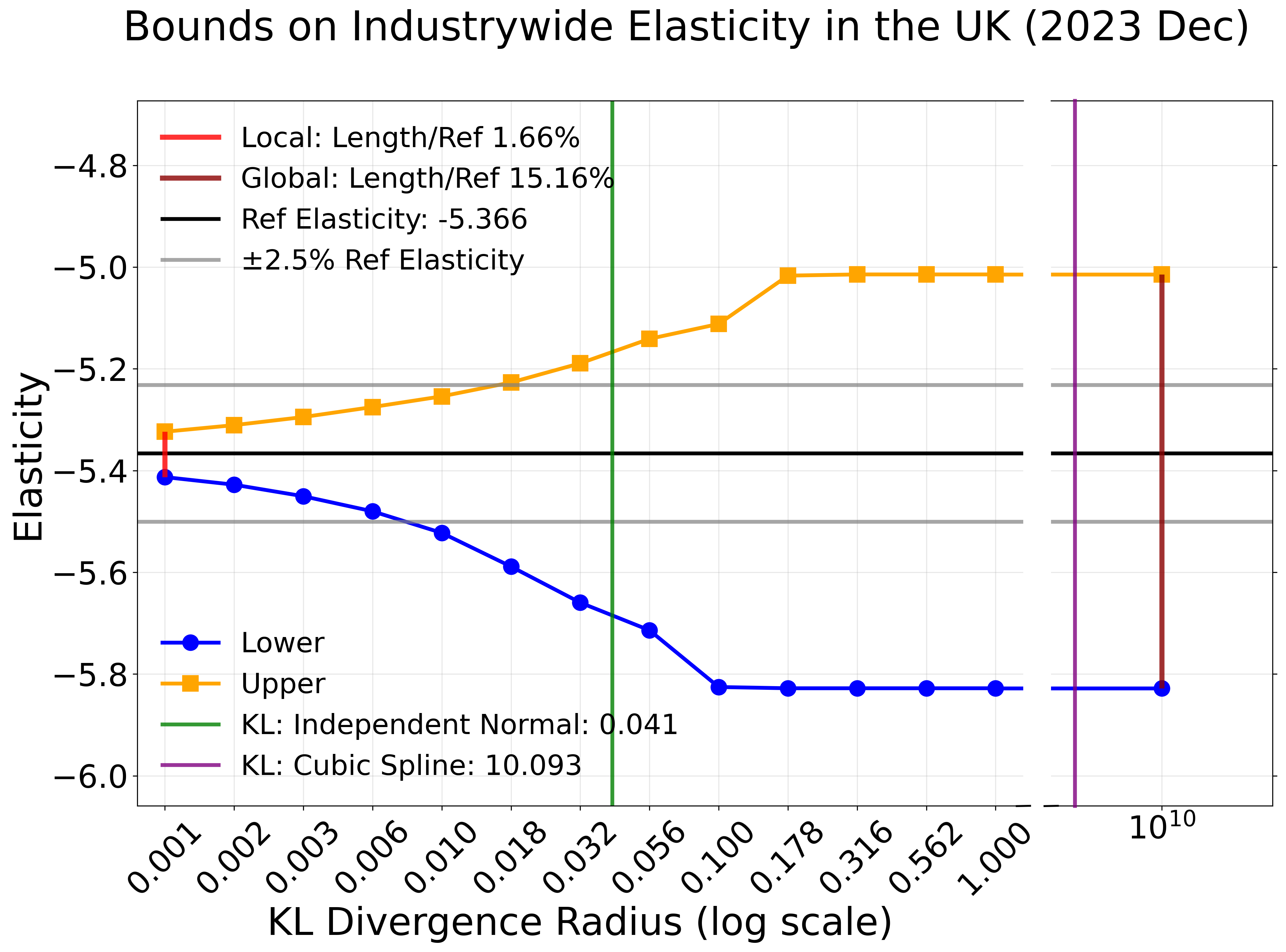
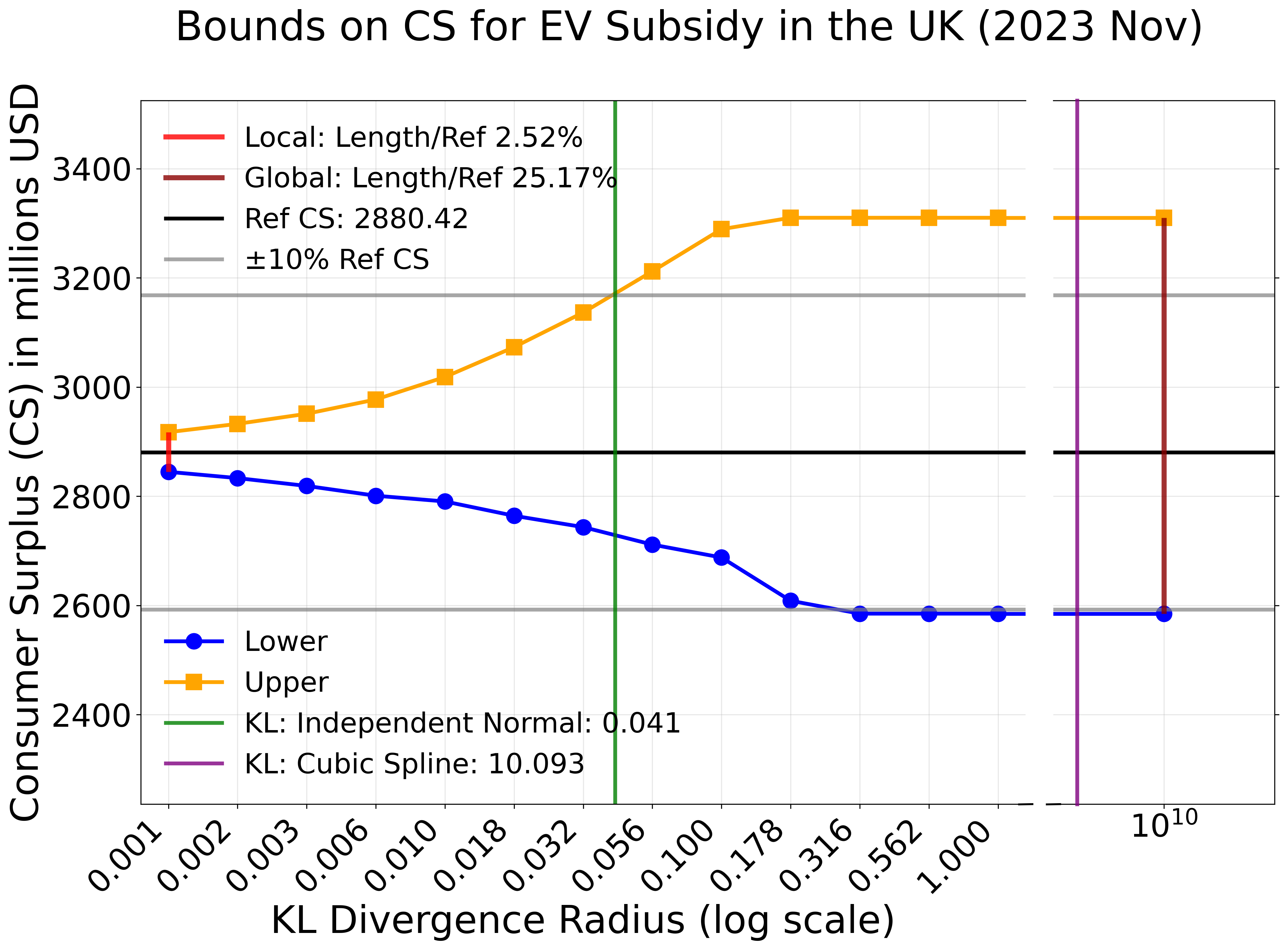
Figure 1: Bounds on Industrywide Elasticity and Consumer Surplus for the UK

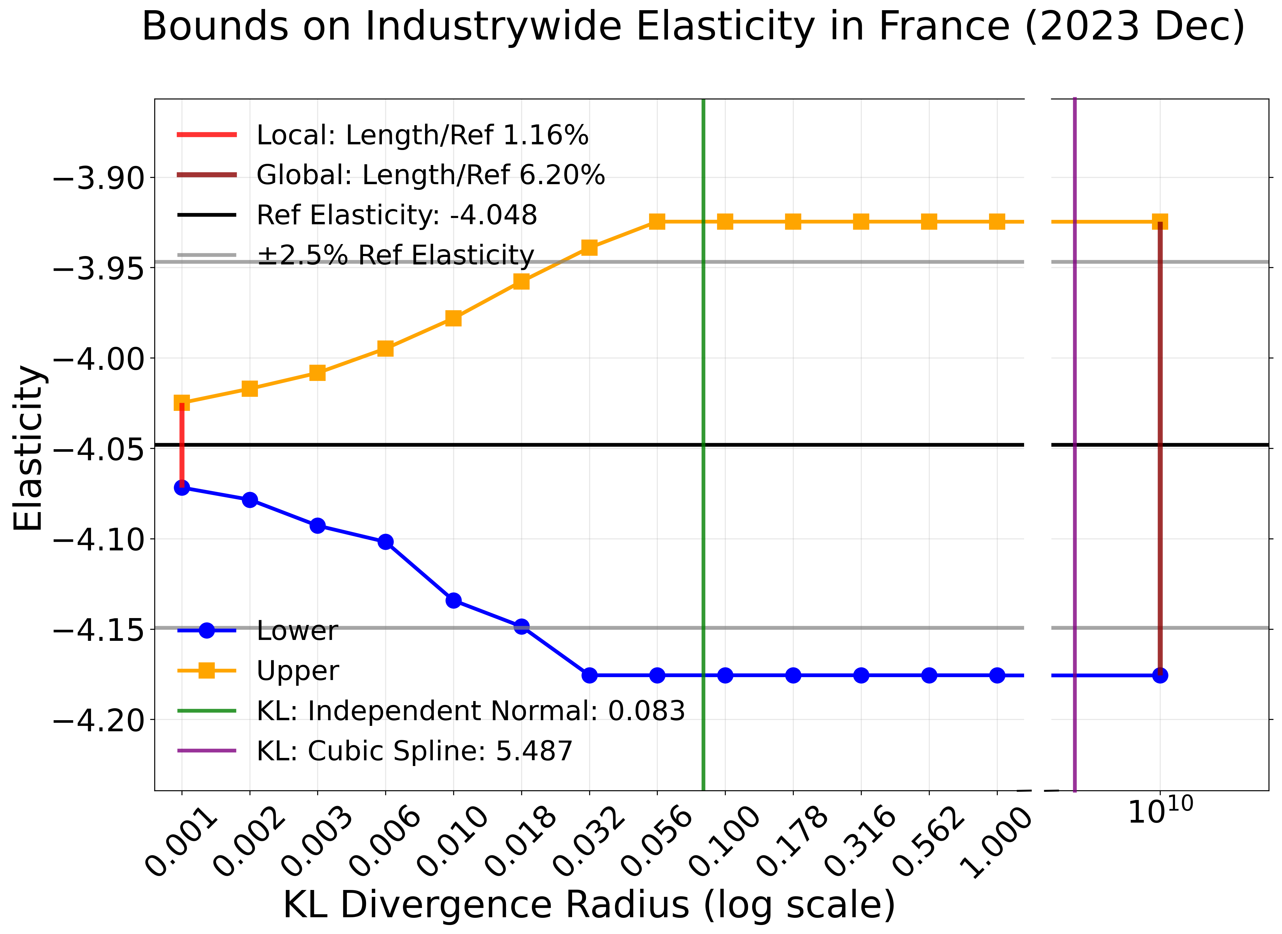
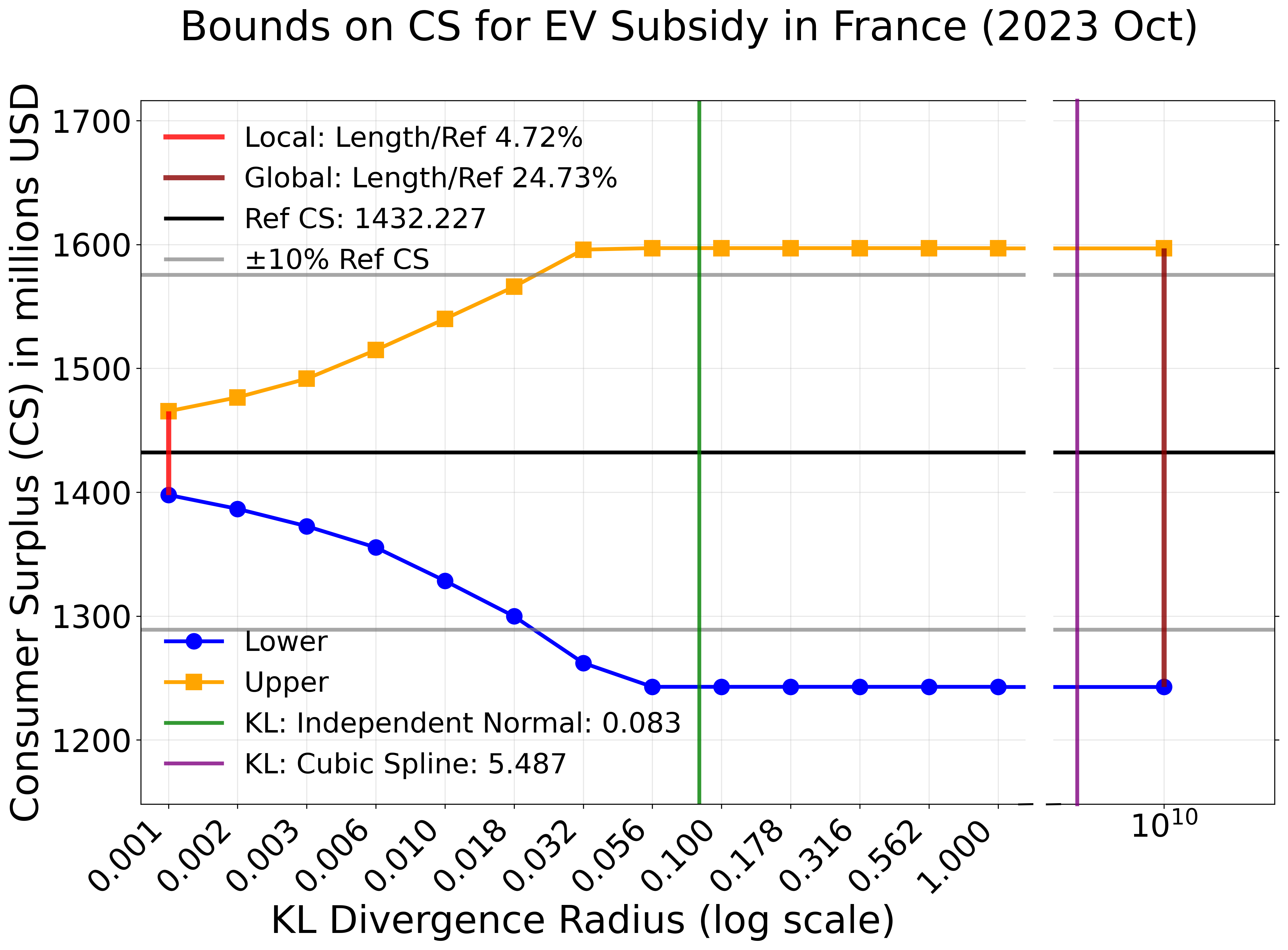
Figure 2: Bounds on Industrywide Elasticity and Consumer Surplus for France

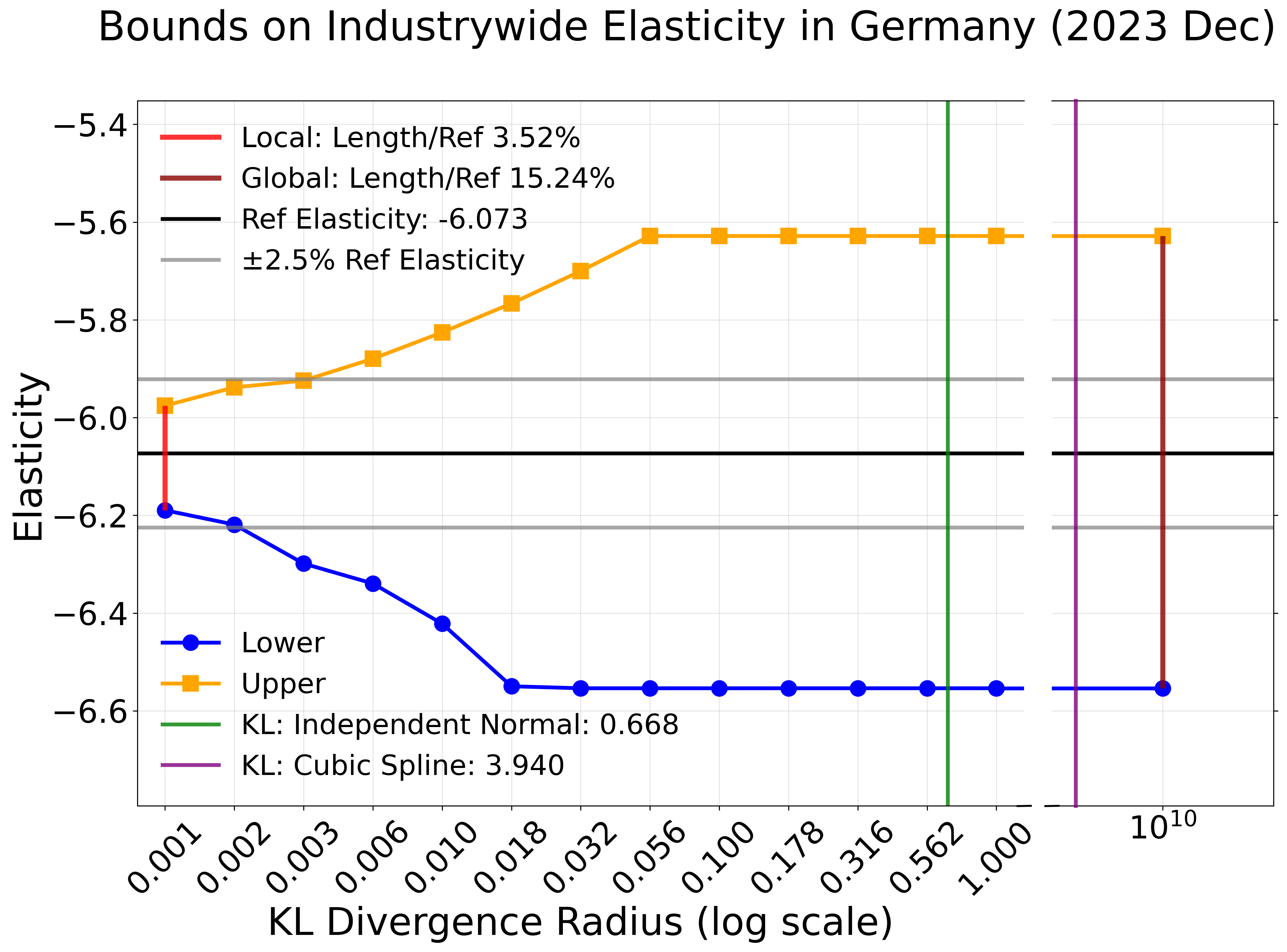
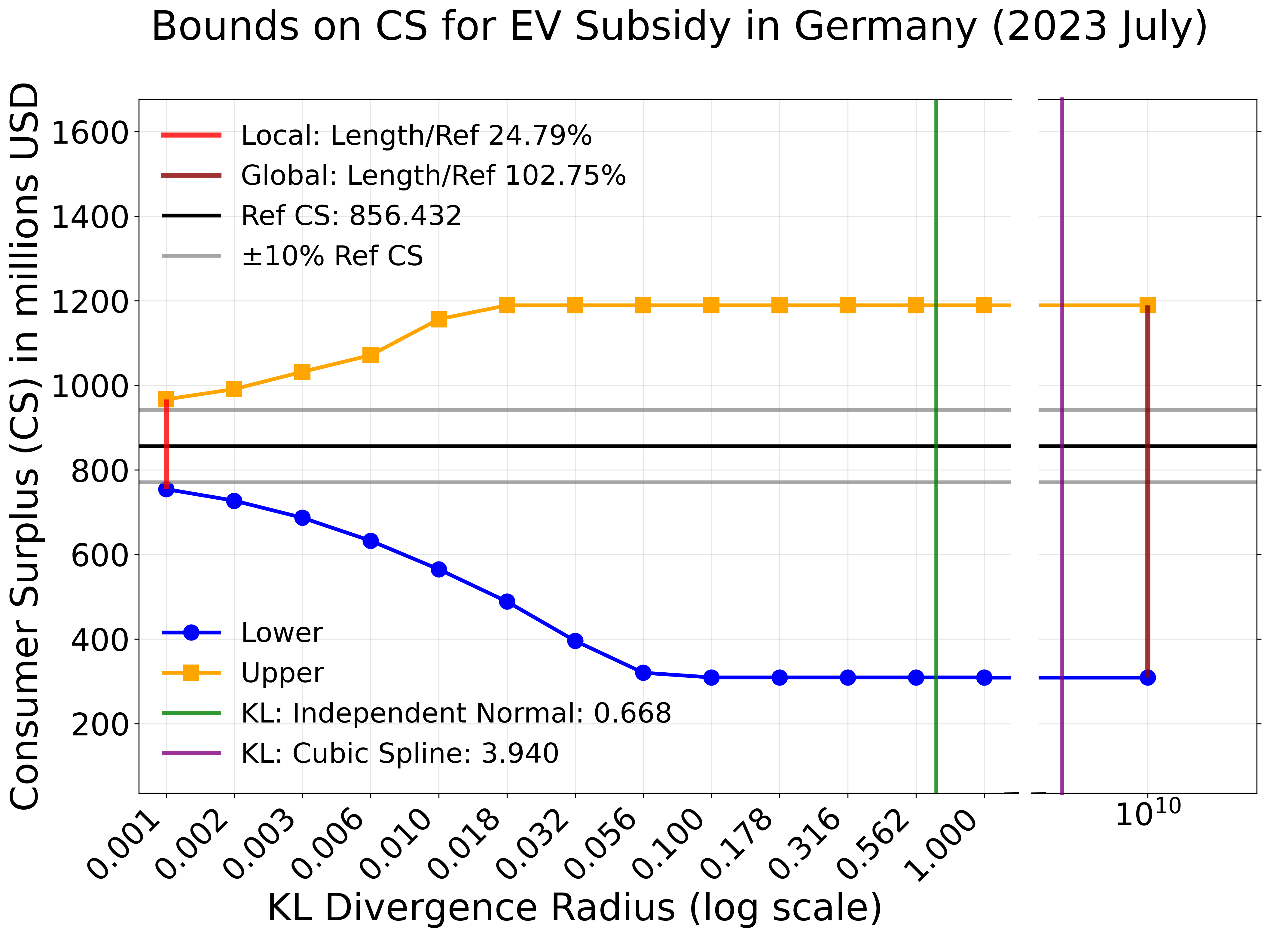
Figure 3: Bounds on Industrywide Elasticity and Consumer Surplus for Germany

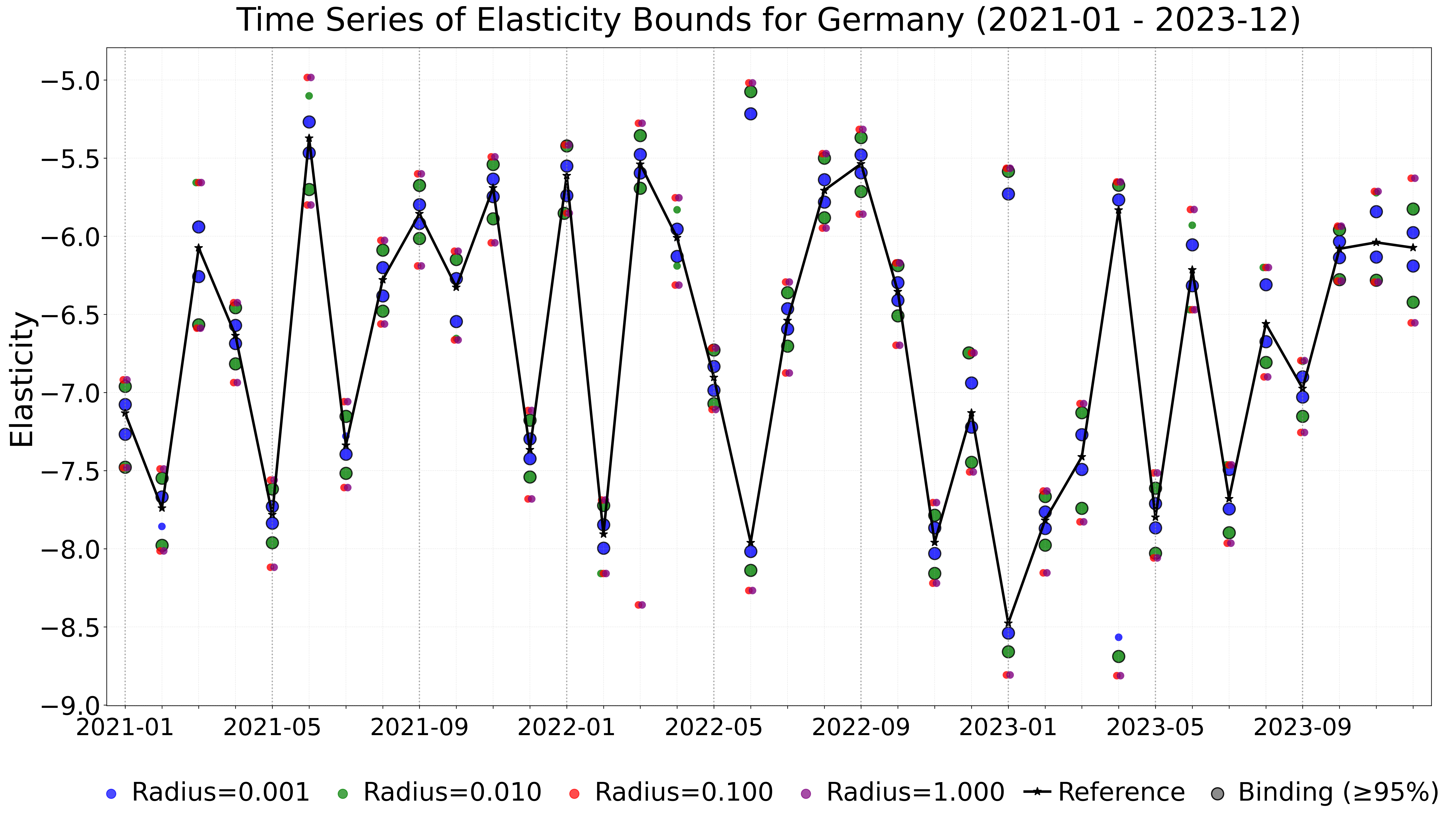
Figure 4: Time Series of Bounds on Industrywide Elasticity for UK, Germany, and France

8 Empirical Application: Finite Horizon DDC

This section applies our framework to a finite-horizon dynamic labor supply model for taxi drivers in New York City (NYC). In the model, the market-level supply shock is the latent variable. Our reference distribution is an AR(1) process. We consider the sensitivity analysis of the labor supply elasticity with respect to such distributional assumptions.

8.1 The Data

We use data from New York City’s Taxi and Limousine Commission’s (TLC) Taxi Passenger Enhancement Project (TPEP). The TPEP data contain a complete record of all trips operated by licensed drivers. The day shift starts at 5 AM and ends at 5 PM, and the night shift starts at 5 PM and ends at 5 AM. We choose a sample of 10,500 drivers that were active in 2013 as in Kalouptsidi et al., 2021c . We restrict the sample to day shift drivers who were only working during the day shifts. We aggregate the transaction-level data to the driver-hour level. In addition, we create 10 uniformly divided bins for weekdays (Monday-Thursday) and 4 bins for weekends (Friday-Sunday) between the lowest and highest hourly earnings and calculate the average hourly earnings in each bin. Then, we remove important days (i.e., Memorial Day, the Fourth of July, and New Year’s Eve). Finally, we restrict the sample to shifts that started between 5 AM and 8 AM, which accounts for 86.84% shifts for weekdays, and 71.84% for weekends. The final sample contains 3,562 drivers and 206 days for weekdays, and 3,322 drivers and 156 days for weekends.

Table 3 presents the hourly summary statistics. The average hourly earnings range from $24.22 at 4:00 PM to $37.00 at 8:00 AM. The share of drivers who continue working is high in the early morning, with 100% of drivers working at 6:00 AM and 7:00 AM. This share starts to decline after 2 PM, and drops substantially to 52.24% and 53.59% by 4:00 PM. Therefore, we assume that drivers can only choose to stop working between 8 AM and 4 PM.

Table 3: Summary statistics.

Hour	Share of Drivers that		Hourly Earnings ($)
	Continue Working (%)		Weekday		Weekend
	Weekday	Weekend	Mean	Std Dev	Mean	Std Dev
6:00 AM	100.00	100.00	32.66	3.00	31.47	3.86
7:00 AM	100.00	100.00	35.04	2.88	30.11	4.49
8:00 AM	98.18	96.21	37.00	2.84	31.21	5.68
9:00 AM	97.64	96.34	34.73	2.37	30.56	4.39
10:00 AM	96.57	96.58	30.02	2.19	30.72	3.33
11:00 AM	95.36	95.80	29.12	2.30	31.48	3.11
12:00 PM	95.53	93.98	30.86	2.26	32.88	2.70
1:00 PM	95.13	94.80	30.62	2.34	33.55	2.65
2:00 PM	92.60	92.84	33.80	2.32	35.02	2.62
3:00 PM	80.61	82.09	34.67	2.02	35.45	2.64
4:00 PM	52.24	53.59	24.22	2.08	25.61	2.40
5:00 PM	0.00	0.00	–	–	–	–
# of Drivers	3,562	3,322
# of Days	206	156

Note: The table uses TPEP Data from January 1, 2013 to December 31, 2013. An observation is defined by a driver-hour.

8.2 The Model

At the beginning of hour $t$ of day $m$, a taxi driver $i$ decides whether to continue working ($a=1$) or not ($a=0$). The decision to stop working is a terminating action, meaning the driver exits the market upon stopping. The period utility of working is given by:

$$u(a_{imt},k_{imt},w_{mt},\xi_{mt},\varepsilon_{imt};\theta)=\begin{cases}\theta_{0}+\theta_{1}k_{imt}+\theta_{2}k_{imt}^{2}+\theta_{3}w_{mt}+\xi_{mt}+\varepsilon_{i1mt}&\text{if }a_{imt}=1\\ \varepsilon_{i0mt}&\text{if }a_{imt}=0\end{cases}$$

where $k_{imt}$ is the number of hours worked, $w_{mt}$ is the average hourly earnings, $\varepsilon_{imt}:=(\varepsilon_{i1mt},\varepsilon_{i0mt})$ is i.i.d. type I extreme value utility shocks, and $\xi_{mt}$ is an exogenously evolved stationary unobserved market-level supply shock. It captures the market-level time-variant unobserved heterogeneity such as weather, congestion, or city events.

We assume markets are i.i.d, and suppress the subscript $(i,m)$ for brevity. Let $u(k_{t},w_{t};\theta)$ be the deterministic part of period of utility of working up to $(\xi_{t},\varepsilon_{t})$. Let $\beta:=0.999999$ be the discount factor. The smoothed Bellman equation at time $t$ is given by:

$$V_{t}(k_{t},w_{t},\xi_{t})=\log\left(\exp\left(v_{0t}(k_{t},w_{t},\xi_{t})\right)+\exp\left(v_{1t}(k_{t},w_{t},\xi_{t})\right)\right)$$

where the conditional value functions of working and not working are given by:

$$v_{1t}(k_{t},w_{t},\xi_{t})=u(k_{t},w_{t};\theta)+\xi_{t}+\beta\mathbb{E}_{\xi_{t+1}|\xi_{t}}\mathbb{E}_{w_{t+1}|w_{t}}[V_{t+1}(k_{t}+1,w_{t+1},\xi_{t+1})]$$ (17)

$$v_{0t}(k_{t},w_{t},\xi_{t})=0$$

8.3 First-Stage Estimation

With only one terminating action, the utility parameters cannot be identified using (11). Therefore, we estimate the utility parameters using the Euler Equations in Conditional Choice Probabilities (ECCP) estimator introduced in Kalouptsidi et al., 2021c . By the Hotz-Miller Inversion Lemma (Hotz and Miller, (1993)), we have:

$$V_{t}(k_{t},w_{t},\xi_{t})=-\log p_{t}(k_{t},w_{t},\xi_{t})=v_{1t}(k_{t},w_{t},\xi_{t})-\log(1-p_{t}(k_{t},w_{t},\xi_{t}))$$ (18)

where $p_{t}(k_{t},w_{t})$ is the CCP of not working. Combining (17) and (18) gives:

$$\log\left(\frac{1-p_{t}(k_{t},w_{t},\xi_{t})}{p_{t}(k_{t},w_{t},\xi_{t})}\right)=u(k_{t},w_{t};\theta)+\xi_{t}-\beta\mathbb{E}_{\xi_{t+1}|\xi_{t}}\mathbb{E}_{w_{t+1}|w_{t}}\left[\log p_{t+1}(k_{t}+1,w_{t+1},\xi_{t+1})\right]$$ (19)

Without a distributional assumption for $\xi_{t}$, we cannot calculate the conditional expectation in (19). However, the cross-sectional data allows us to estimate CCPs, denoted as $\hat{p}_{t}(k,w)$. We estimate $\hat{p}_{t}(k,w)$ by a flexible logit for each $t$. Let the expectational error be:

$$\hat{e}(k_{t},w_{t},k_{t+1},w_{t+1},\xi_{t}):=\beta\log\hat{p}_{t+1}(k_{t+1},w_{t+1})-\beta\mathbb{E}_{\xi_{t+1}|\xi_{t}}\mathbb{E}_{w_{t+1}|w_{t}}\left[\log p_{t+1}(k_{t+1},w_{t+1},\xi_{t+1})\right]$$

where $k_{t+1}=k_{t}+1$. Then, we can rewrite (19) as:

$$\log\left(\frac{1-\hat{p}_{t}(k_{t},w_{t})}{\hat{p}_{t}(k_{t},w_{t})}\right)+\beta\log\hat{p}_{t+1}(k_{t+1},w_{t+1})=u(k_{t},w_{t};\theta)+\xi_{t}+\hat{e}(k_{t},w_{t},k_{t+1},w_{t+1},\xi_{t})$$

Therefore $\theta$ can be identified using an instrument for $\xi_{t}+\hat{e}(k_{t},w_{t},k_{t+1},w_{t+1},\xi_{t})$. Denote by $\mathcal{K}_{t}$ the set of possible hours worked at $t$. The ECCP estimator stacks all $k\in\mathcal{K}_{t}$. A unit of observation is defined by day-hour.

Following Kalouptsidi et al., 2021c , we use the previous day’s average hourly earnings for the same hour as the IV. Table 4 shows the estimation results. The implied marginal value of time defined by $-\frac{\theta_{1}+2\theta_{2}k}{\theta_{3}}$ ranges from $0 at around $k=7$ hours to $5.35 at $k=11$ hours for weekdays, and from $0 at around $k=8$ hours to $9.95 at $k=11$ hours for weekends.

Table 4: ECCP Estimation Results

	Model Estimates
	Weekday		Weekend
Variable	Coef.	Std. Err.	Coef.	Std. Err.
Constant	$-2.1720$	$(0.0304)$	$-0.5631$	$(0.0724)$
Hours worked	$\phantom{-}0.4035$	$(0.0025)$	$\phantom{-}0.1866$	$(0.0032)$
Hours worked (squared)	$-0.0274$	$(0.0002)$	$-0.0116$	$(0.0003)$
Average hourly earnings	$\phantom{-}0.0373$	$(0.0010)$	$\phantom{-}0.0069$	$(0.0023)$
# of Drivers	3,562		3,322
# of Days	206		156

Notes: A unit of observation is defined by day-hour. Each observation stacks all $k_{t}\in\mathcal{K}_{t}$. The model is estimated using 2SLS with the previous day’s average hourly earnings as the IV. The standard errors are clustered at the day-$k$ level.

8.4 The Reference Distribution and Scalar Parameters of Interest

We define the reference distribution and introduce the scalar parameters of interest. Let $N_{tk}$ be the number of drivers who has worked $k$ hours at hour $t$. The market-level $\xi_{t}$ equates the model-implied weighted average CCP of not working with the observed weighted average:

$$\sum_{k\in\mathcal{K}_{t}}\frac{N_{tk}}{\sum_{k\in\mathcal{K}_{t}}N_{tk}}p_{t}(k,w_{t},\xi_{t})=\sum_{k\in\mathcal{K}_{t}}\frac{N_{tk}}{\sum_{k\in\mathcal{K}_{t}}N_{tk}}\hat{p}_{t}(k,w_{t})$$ (20)

As we assume $\xi_{t}$ is stationary, its marginal distribution at $T$ is its stationary distribution. At hour $T$, drivers solve a static problem, and the CCP of not working is:

$$p_{T}(k_{T},w_{T},\xi_{T})=\frac{1}{1+\exp\left(u(k_{T},w_{T},\xi_{T})\right)}$$

Therefore, the stationary distribution is identified by recovering $\xi_{T}$ to satisfy (20) at $T$. Figure 5 plots the kernel density estimator of $\xi_{T}$. We fit a Gaussian distribution to the last period $\xi_{T}$. Denote its mean and standard deviation as $\mu_{\xi}$ and $\sigma_{\xi}$, respectively.

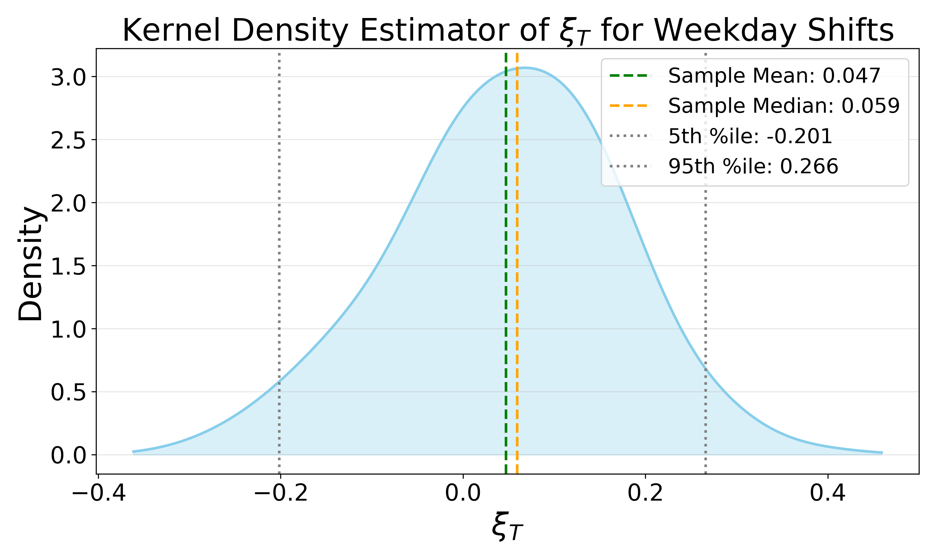
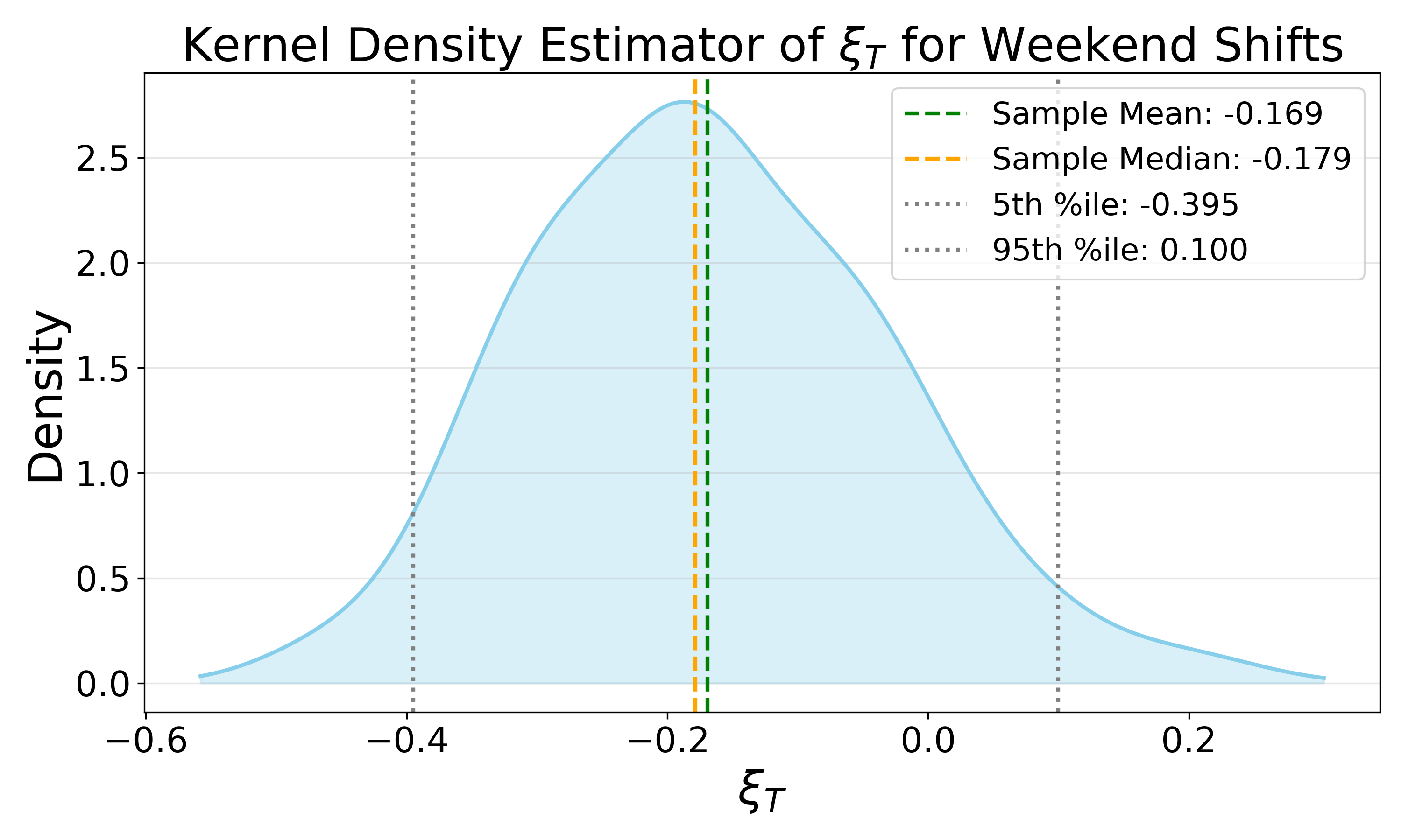
Figure 5: Kernel Density Estimator of the Last Period $\xi_{T}$

The reference model for $\xi_{t}$ is an AR(1) process:

$$\xi_{t}=\mu+\rho\xi_{t-1}+\eta_{t}$$ (21)

where $\eta_{t}$ follows i.i.d normal distribution with mean 0 and variance $\sigma^{2}$. As we have identified its stationary distribution, we only need to solve the fixed point problem for $\rho$: we begin with an initial guess of $\rho$ and circulate between: (i) setting $\mu=\mu_{\xi}\cdot(1-\rho)$ and $\sigma=\sigma_{\xi}\cdot\sqrt{1-\rho^{2}}$, (ii) solving the Bellman equation using backward induction, (iii) recovering $\xi_{t}$ using (20), and (iv) updating $\rho$ by refitting the AR(1) process to the recovered $\xi_{t}$ until convergence. The reference distribution $F_{0}$ for $(\xi,\xi^{\prime})$ is the product of the transition kernel of the estimated AR(1) process and its stationary distribution $\nu_{0}$. The perturbation set is defined as:

$$\mathcal{F}:=\left\{F\in\mathcal{P}(\mathcal{U})\mid F\in\Pi(\nu_{0},\nu_{0}),D_{KL}(F\|F_{0})\leq\delta\right\}$$

We consider two scalar parameters of interest: the elasticity of stopping working, and the Frisch elasticity of labor supply. Both elasticities are at the individual level, meaning the demand side remains unchanged. Therefore, we keep the transitions of $w_{t}$ and $\xi_{t}$ fixed.

For the elasticity of stopping working, we increase the average hourly earnings from the current bin, $w_{mt}$, to the next bin, $w^{\prime}_{mt}$. The weighted average of the elasticity at hour $t$ is:

$$\sum_{m}\sum_{k\in\mathcal{K}_{mt}}\frac{N_{mtk}}{\sum_{m,k\in\mathcal{K}_{mt}}N_{mtk}}\frac{p_{t}(k,w^{\prime}_{mt},\xi_{mt})-\hat{p}_{kmt}}{\hat{p}_{kmt}}\times\frac{w^{\prime}_{mt}-w_{mt}}{w_{mt}}$$

As shown in Table 3, the share of drivers who continue working begins to decline around 11 AM.Moreover, our model does not endogenize the initial entry decision (i.e., the choice of when to start a shift). To compute the Frisch elasticity, we assume 11 AM is the first hour drivers can choose to stop working, and consider a 1% increase in average hourly earnings beginning at 11 AM. The total expected hours worked at day $m$ is:

$$H(m,\bm{\xi}_{m},\bm{w}_{m},p):=\sum_{k\in\{3,4,5,6\}}N_{mk}\sum_{t=12}^{16}(t-11)p_{mt}(k,w_{mt},\xi_{mt})\Pi_{t_{1}=11}^{t-1}(1-p_{t_{1}}(k,w_{mt_{1}},\xi_{mt_{1}}))$$

where $N_{mk}$ is the number of drivers whose hours worked is $k$ at 11 AM of day $m$, and $\bm{\xi}_{m},\bm{w}_{m}$ are the vectors of $\xi_{mt},w_{mt}$ for $t=11,\ldots,16$. Then, the Frisch elasticity is:

$$\frac{\sum_{m}H(m,\bm{\xi}_{m},\bm{w}^{\prime}_{m},p^{\prime})-\sum_{m}H(m,\bm{\xi}_{m},\bm{w}_{m},p)}{\sum_{m}H(m,\bm{\xi}_{m},\bm{w}_{m},p)}\times 100$$

where $\bm{w}^{\prime}_{m}=1.01\cdot\bm{w}_{m}$, and $p^{\prime}$ is derived from the Bellman equation with $\bm{w}^{\prime}_{m}$.

8.5 Sensitivity Analysis

We convert (19) into an unconditional moment constraint by assuming that $p_{t}(k,w,\xi)$ is the solution to (19) for given $p_{t+1}(k+1,w,\xi)$ if and only if:

$$\sup_{g_{tk}\in C(\mathcal{W}\times\Xi)}\mathbb{E}_{F}\mathbb{E}_{w_{t+1},w_{t}}\left[g_{tk}(w_{t},\xi_{t})\left(\log\left(\frac{1-p_{t}(k,w_{t},\xi_{t})}{p_{t}(k,w_{t},\xi_{t})}\right)-u(k,w_{t})-\xi_{t}+\beta\log p_{t+1}(k+1,w_{t+1},\xi_{t+1})\right)\right]$$ (22)

Let the term inside the expectation in (22) be $\psi_{t}(k,w_{t},w_{t+1},\xi_{t},\xi_{t+1};u,p_{t},p_{t+1},g_{tk})$.

To profile out $\xi_{mt}$ from recovering the probability of stop working, we assume:

Assumption 13.

For $\forall\ F\in\mathcal{F}$, the solution $p_{tk}(w,\xi)$ corresponding to (22) satisfies the following: for all $m,t$, there exists a unique $\xi_{mt}\in\Xi$ that satisfies (20).

The final constraint is a fixed point constraint similar to the procedure used to estimate the AR(1) process. Suppose $F$ is used in (22). Denote by $\hat{F}$ an estimator of the distribution of the pair $(\xi,\xi^{\prime})$ using the recovered $\{\xi_{mt}\}_{m=1,t=1}^{M,T-1}$ from (20). Then, our fixed point constraint is:

$$D_{KL}(F\|\hat{F})\leq\epsilon_{M}$$

where $\epsilon_{M}$ is the tolerance level. As the sample size is large, we use Scott’s Rule to initialize the bandwidth and then use 5-fold cross-validation to select bandwidth candidates around Scott’s estimate that maximizes the log-likelihood. To choose $\epsilon_{M}$, we estimate the joint distribution of supply shocks recovered from the AR(1) process by the kernel density estimator with Gaussian kernel. Then, we set $\epsilon_{M}$ to be the KL divergence between the kernel density estimator and the reference distribution.

Then, the lower bound on the elasticity of stopping working at $t$ is:

$$\inf_{\{p_{t}\}_{t=1}^{T-1}}\inf_{F\in\mathcal{F}} \quad\sum_{m}\sum_{k\in\mathcal{K}_{mt}}\frac{N_{mtk}}{\sum_{m,k\in\mathcal{K}_{mt}}N_{mtk}}\frac{p_{t}(k,w^{\prime}_{mt},\xi_{mt})-\hat{p}_{kmt}}{\hat{p}_{kmt}}\times\frac{w^{\prime}_{mt}-w_{mt}}{w_{mt}}$$

s.t. $$\sum_{k\in\mathcal{K}_{mt}}\frac{N_{mtk}}{\sum_{k\in\mathcal{K}_{mt}}N_{mtk}}p_{t}(k,w_{mt},\xi_{mt})=\sum_{k\in\mathcal{K}_{mt}}\frac{N_{mtk}}{\sum_{k\in\mathcal{K}_{mt}}N_{mtk}}\hat{p}_{t}(k,w_{mt})\text{ for }\forall\ m,t$$

$$\sup_{g_{tk}}\mathbb{E}_{F}\mathbb{E}_{w_{t+1},w_{t}}\left[\psi_{t}(k,\xi_{t},\xi_{t+1},w_{t},w_{t+1};u,p_{t},p_{t+1},g_{tk})\right]\text{ for }\forall\ t\leq T-1,k$$ (23)

$$D_{KL}(F\|\hat{F})\leq\epsilon_{M}$$

The last period $T$ is a static problem, therefore $p_{T}$ is not an optimization parameter. For $\delta=0$, the reference distribution is the unique solution to the above problem. The corresponding elasticity is the reference elasticity.

For the Frisch elasticity, we increase the earnings coefficient by 1% from 11 AM. This allows us to leave the discretized state space and its transition unchanged at the cost of solving additional Bellman equations. The lower bound on the Frisch elasticity is:

$$\inf_{\{p_{t},p^{\prime}_{t}\}_{t=1}^{T-1}}\inf_{F\in\mathcal{F}} \quad\frac{\sum_{m}H(m,\bm{\xi}_{m},\bm{w}^{\prime}_{m},p^{\prime})-\sum_{m}H(m,\bm{\xi}_{m},\bm{w}_{m},p)}{\sum_{m}H(m,\bm{\xi}_{m},\bm{w}_{m},p)}\times 100$$

s.t. $$\sum_{k\in\mathcal{K}_{mt}}\frac{N_{mtk}}{\sum_{k\in\mathcal{K}_{mt}}N_{mtk}}p_{t}(k,w_{mt},\xi_{mt})=\sum_{k\in\mathcal{K}_{mt}}\frac{N_{mtk}}{\sum_{k\in\mathcal{K}_{mt}}N_{mtk}}\hat{p}_{t}(k,w_{mt})\text{ for }\forall\ m,t$$

$$\sup_{g^{1}_{tk}}\mathbb{E}_{F}\mathbb{E}_{w_{t+1},w_{t}}\left[\psi_{t}(k,\xi_{t},\xi_{t+1},w_{t},w_{t+1};u,p_{t},p_{t+1},g^{1}_{tk})\right]\text{ for }\forall\ t\leq T-1,k$$

$$\sup_{g^{2}_{tk}}\mathbb{E}_{F}\mathbb{E}_{w_{t+1},w_{t}}\left[\psi_{t}(k,\xi_{t},\xi_{t+1},w_{t},w_{t+1};u^{\prime},p_{t},p_{t+1},g^{2}_{tk})\right]\text{ for }\forall\ t\leq T-1,k$$

$$D_{KL}(F\|\hat{F})\leq\epsilon_{M}$$

where $u^{\prime}$ is the utility function with the earning coefficient increased by 1% from 11 AM.

8.6 Implementation

We adjust the procedure in Section 7.6 to account for the finite horizon model. The main difference is that we solve the Bellman equation (19) by backward induction. The number of Bellman equations (23) is 31. The number of optimization parameters is $31\cdot N_{w}N_{\xi}+1$ for the elasticity of stopping working, and $62\cdot N_{w}N_{\xi}+1$ for the Frisch elasticity, where $N_{w}$ is the number of bins for average hourly earnings, $N_{\xi}$ is the number of grid points for $\xi$, and 1 is for the KL divergence constraint. We choose $N_{\xi}=99$, 5,000 MCMC steps for Frisch elasticities, 2,500 MCMC steps for elasticities of stopping working, 5 optimization steps, 14 radii (the last is $10^{10}$), and 100 as the simulated annealing multiplier. The covariance matrix for the random walk in Algorithm 1 is restricted to be diagonal.

8.7 Results

The alternative model is an independent model where the supply shocks are i.i.d. and follow the stationary distribution identified at $T$. The independent model is closer to the reference model for weekends than for weekdays. The KL divergence between the independent model and the reference model is 0.115 for weekends and 3.673 for weekdays.

Figure 6 plots the elasticity of stopping working from 9 AM to 3 PM for weekdays and weekends. We set $\delta=0.001$ for local deviation and $\delta=1$ for global deviation. Large points indicate that the KL divergence constraint is binding. When two consecutive points align horizontally, this indicates that increasing the radius does not affect the bounds. The elasticity of stopping working is negative and decreases over time. In particular, the labor supply is inelastic before 11 AM on weekdays and 12 PM on weekends, and elastic after that. At 3 PM, the elasticity of stopping working is around -2 for weekdays and -2.5 for weekends. Overall, both weekday and weekend elasticities are not sensitive to the distributional assumption. For weekdays, elasticity in the morning is more sensitive than in the afternoon in terms of both local and global sensitivity, while it is the opposite for weekends.

Figure 7 plots the Frisch elasticity bounds for weekdays and weekends. The reference Frisch elasticity is 0.472 for weekends and 0.698 for weekdays. Our reference estimates are consistent with labor supply literature. For example, Buchholz et al., (2023) reports a Frisch elasticity ranging from 0.47-0.54 for NYC taxi drivers. For both weekdays and weekends, the bounds flatten around 0.032-0.056. In terms of local sensitivity, the results appear sensitive to the distributional assumption, with a deviation of 28.37% for weekdays and 21.76% for weekends. In terms of global sensitivity, the deviation is larger, with 76.83% for weekdays and 42.84% for weekends. For the robustness metric approach, we consider a 15% deviation from the reference Frisch elasticity. The weekday’s robustness metric is around 0.001 for the upper bound, while the lower bound never reaches the 15% deviation. The weekend’s robustness metric is around 0.008 for the upper bound, and 0.01 for the lower bound. Therefore, the weekday’s lower bound is more robust than the weekend’s lower bound, while the weekday’s upper bound is less robust than the weekend’s upper bound.

Figure 6: Elasticity of Stopping Working by Hour of Day for NYC Taxi Drivers

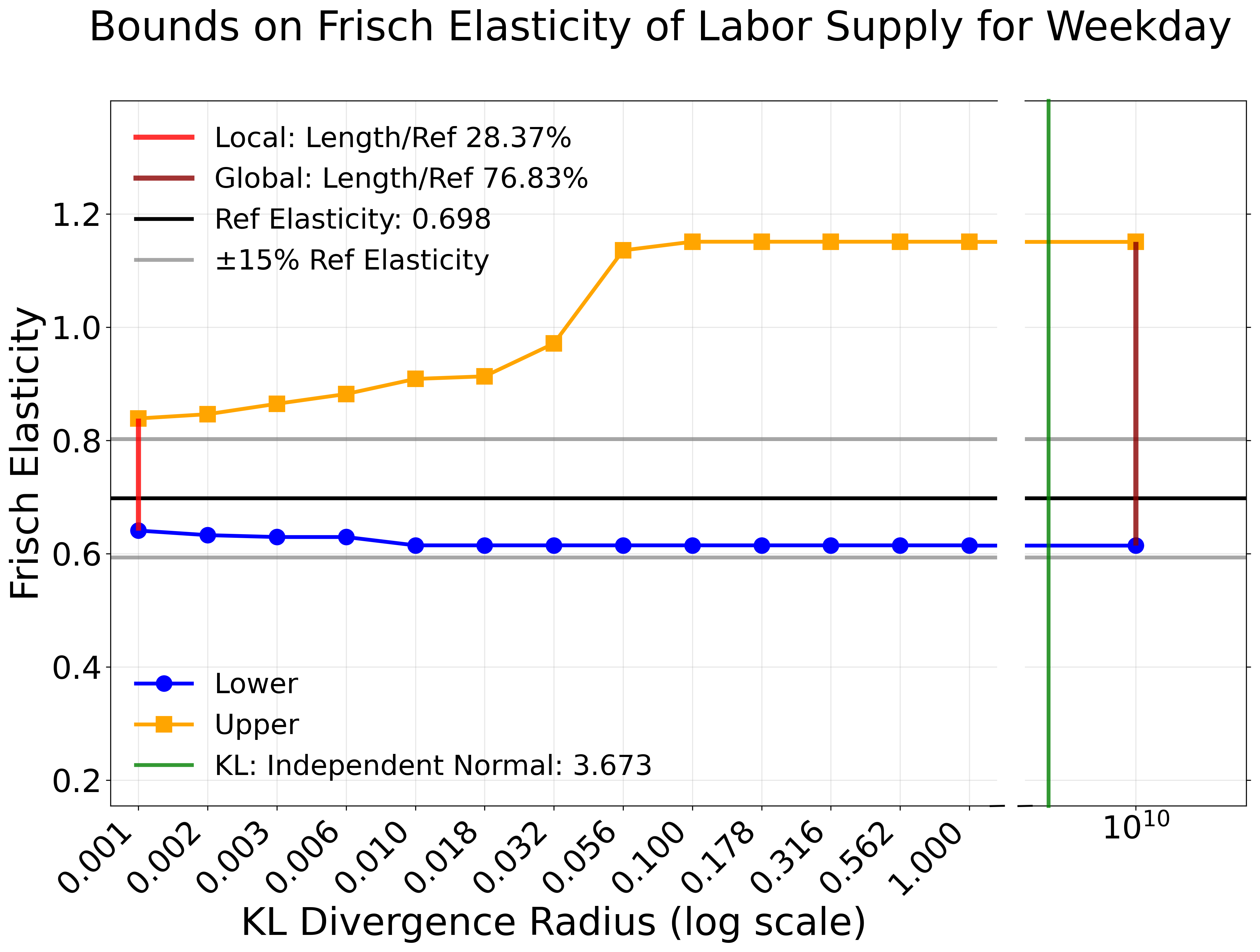
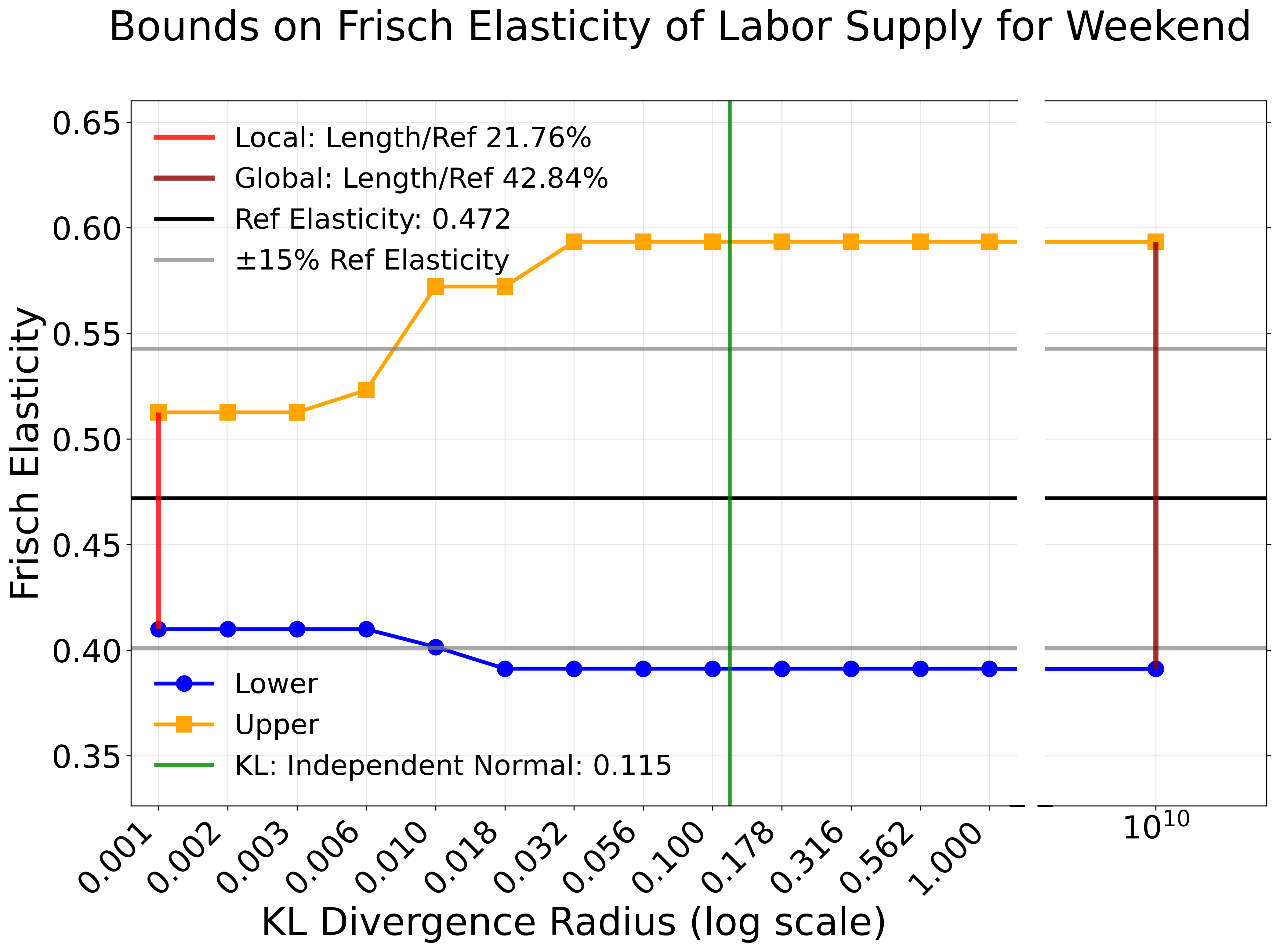
Figure 7: Frisch Elasticity Bounds by Hour of Day for NYC Taxi Drivers

9 Conclusion

This paper proposes a computationally tractable framework to quantify the sensitivity of outcomes of interest to distributional assumptions about the serial dependence of latent variables in dynamic structural models. We derive bounds on a scalar parameter of interest by perturbing a reference transition distribution, while imposing a stationarity condition for time-homogeneous models or a Markovian condition for time-inhomogeneous models. We apply the approach to an infinite-horizon dynamic demand model for new cars in the UK, Germany, and France, and a finite-horizon dynamic labor supply model for taxi drivers in New York City.

Appendix A Additional Examples

Example 4 (Infinite Horizon Dynamic Discrete Choice Models).

This example considers the serial independence assumption on utility shocks in a single-agent DDC model, as in Rust, (1987). Agents solve the Bellman equation for the conditional value function $v\in\mathcal{V}$:

$$v_{j}(x,\varepsilon)=\pi_{j}(x,\varepsilon;\theta)+\beta\mathbb{E}_{\varepsilon^{\prime}|\varepsilon}\mathbb{E}_{x^{\prime}|x,j}\max_{j^{\prime}\in\mathcal{J}}v_{j^{\prime}}(x^{\prime},\varepsilon^{\prime})$$ (24)

where $\varepsilon\in\mathbb{R}^{J}$ is a vector of utility shocks for each action $j\in\mathcal{J}$, $x\in\mathcal{X}$ is the observable state variable, $\beta\in(0,1)$ is the discount factor, $\pi_{j}(x,\varepsilon;\theta)$ is the period utility parameterized by $\theta\in\Theta$, and $\mathcal{V}$ is the class of conditional value functions.

Let $U:=(\varepsilon,\varepsilon^{\prime})$ be a vector of current and future utility shocks. The serial independence is often imposed on utility shocks, which implies a reference distribution:

$$dF_{0}(U):=\nu_{0}(d\varepsilon)\nu_{0}(d\varepsilon^{\prime})$$

whose perturbation set is defined as:

$$\mathcal{F}:=\left\{F\in\mathcal{P}(\mathcal{U})\mid F\in\Pi(\nu_{0},\nu_{0}),D_{KL}(F\|F_{0})\leq\delta\right\}$$

Suppose the scalar parameter of interest is the social welfare, defined as:

$$\mathbb{E}_{\nu_{0}}\mathbb{E}_{x}\max_{j\in\mathcal{J}}v_{j}(x,\varepsilon)$$

We convert the Bellman equation (24) into a restriction that depends on the joint distribution $F\in\mathcal{F}$. We assume there exists a class of Lagrange multiplier functions $\mathcal{G}$ such that $v$ solves the Bellman equation (24) if and only if:

$$\sup_{g\in\mathcal{G}}\mathbb{E}_{F}\mathbb{E}_{x,j,x^{\prime}}\left[g_{j}(x,\varepsilon)\left(v_{j}(x,\varepsilon)-\pi_{j}(x,\varepsilon;\theta)-\beta\max_{j^{\prime}\in\mathcal{J}}v_{j^{\prime}}(x^{\prime},\varepsilon^{\prime})\right)\right]=0$$

We can rewrite the structural constraint as:

$$\sup_{g\in\mathcal{G}}\mathbb{E}_{F}\left[\psi(U;\theta,v,g)\right]=0$$

where $\psi(U;\theta,v,g):=\mathbb{E}_{x,j,x^{\prime}}\left(g_{j}(x,\varepsilon)\left(v_{j}(x,\varepsilon)-\pi_{j}(x,\varepsilon;\theta)-\beta\max_{j^{\prime}\in\mathcal{J}}v_{j^{\prime}}(x^{\prime},\varepsilon^{\prime})\right)\right)$.

We consider the following moment conditions for estimation:

$$\mathbb{E}_{F}\mathbbm{1}(v_{j}(x,\varepsilon)=\max_{j^{\prime}\in\mathcal{J}}v_{j^{\prime}}(x,\varepsilon))=P_{0}(j|x)\quad\forall\ (j,x)\in\mathcal{J}\times\mathcal{X}$$

where $\mathbbm{1}$ is the indicator function, and $P_{0}(j|x)$ is the population CCP. We assume $\mathcal{X}$ has discrete support, and rewrite the moment conditions as:

$$\mathbb{E}_{F}\left[m(U;v)\right]=P_{0}$$

where $m(U;v)$ stacks the indicator functions for each $(x,j)$ given $v$, and $P_{0}$ stacks the CCPs.

Then, the lower bound on the social welfare is given by:

$$\inf_{(\theta,v,F)\in\Theta\times\mathcal{V}\times\mathcal{F}} \mathbb{E}_{\nu_{0}}\mathbb{E}_{x}\max_{j\in\mathcal{J}}v_{j}(x,\varepsilon)$$

s.t. $$\mathbb{E}_{F}\left[m(U;v)\right]=P_{0}$$

$$\sup_{g\in\mathcal{G}}\mathbb{E}_{F}\left[\psi(U;\theta,v,g)\right]=0$$

Example 5 (Infinite Horizon Dynamic Discrete-Continuous Choice Models).

This example considers the serial independence assumption on the consumption shock in a single-agent dynamic discrete-continuous choice model, as in Iskhakov et al., (2017) and Levy and Schiraldi, (2022). At each period, individuals make a discrete choice $j\in\mathcal{J}$, and a continuous choice $q\in\mathbb{R}$. The value function solves the Bellman equation:

$$V(x,I,\xi,\varepsilon)=\max_{j,q}\left\{\pi_{j}(q,x,I,\xi;\theta)+\varepsilon_{j}+\beta\mathbb{E}_{\xi^{\prime}|\xi}\mathbb{E}_{x^{\prime}|x,j}V(x^{\prime},I^{\prime},\xi^{\prime},\varepsilon^{\prime})\right\}$$

where $I$ is the resource constraint (e.g., inventory) evolving deterministically over time according to $I^{\prime}=L(x,I,q,j)$, $x\in\mathcal{X}$ is the observable state variable, $\varepsilon\in\mathbb{R}^{J}$ is a vector of i.i.d. Extreme Value Type I utility shocks, $\xi\in\Xi$ is the consumption shock, $\pi_{j}(q,x,I,\xi;\theta)$ is the period utility parameterized by $\theta\in\Theta$, and $\beta\in(0,1)$ is the discount factor.

Let $q^{*}_{j}:=q^{*}_{j}(x,I,\xi)$ be the conditional optimal continuous choice for $(j,x,I,\xi)$. Given $q^{*}_{j}$, the conditional value function $v_{j}\in\mathcal{V}$ solves:

$$v_{j}(x,I,\xi)=\pi_{j}(q^{*}_{j},x,I,\xi;\theta)+\beta\mathbb{E}_{\xi^{\prime}|\xi}\mathbb{E}_{x^{\prime}|x,j}\left[\log\left(\sum_{j^{\prime}\in\mathcal{J}}\exp\left(v_{j^{\prime}}(x^{\prime},I^{\prime},\xi^{\prime})\right)\right)\right]+\beta\gamma$$ (25)

The model-implied conditional choice probability is given by:

$$p(j|x,I,\xi)=\frac{\exp\left(v_{j}(x,I,\xi)\right)}{\sum_{j^{\prime}\in\mathcal{J}}\exp\left(v_{j^{\prime}}(x,I,\xi)\right)}$$

We assume that the optimal continuous choice is attained at an interior point and the dominated convergence theorem holds. Therefore, the first-order condition for (25) holds:

$$\frac{\partial\pi_{j}(q^{*}_{j},x,I,\xi;\theta)}{\partial q}+\beta\mathbb{E}_{\xi^{\prime}|\xi}\mathbb{E}_{x^{\prime}|x,j}\left[\sum_{j^{\prime}\in\mathcal{J}}p(j^{\prime}|x^{\prime},I^{\prime},\xi^{\prime})\frac{\partial v_{j^{\prime}}(x^{\prime},I^{\prime},\xi^{\prime})}{\partial I^{\prime}}\right]\frac{\partial L(x,I,q^{*}_{j},j)}{\partial q}=0$$

By the envelope theorem, we have:

$$\frac{\partial v_{j^{\prime}}(x^{\prime},I^{\prime},\xi^{\prime})}{\partial I^{\prime}}=\frac{\partial\pi_{j^{\prime}}(q^{*}_{j^{\prime}},x^{\prime},I^{\prime},\xi^{\prime};\theta)}{\partial q}$$

Therefore, the Euler equation for the optimal continuous choice is:

$$\frac{\partial\pi_{j}(q^{*}_{j},x,I,\xi;\theta)}{\partial q}+\beta\mathbb{E}_{\xi^{\prime}|\xi}\mathbb{E}_{x^{\prime}|x,j}\left[\sum_{j^{\prime}\in\mathcal{J}}p(j^{\prime}|x^{\prime},I^{\prime},\xi^{\prime})\frac{\partial\pi_{j^{\prime}}(q^{*}_{j^{\prime}},x^{\prime},I^{\prime},\xi^{\prime};\theta)}{\partial q}\right]\frac{\partial L(x,I,q^{*}_{j},j)}{\partial q}=0$$ (26)

Let $U:=(\xi,\xi^{\prime})$ be a vector of current and future consumption shocks. The serial independence is often imposed on consumption shocks, which implies a reference distribution:

$$dF_{0}(U):=\nu_{0}(d\xi)\nu_{0}(d\xi^{\prime})$$

whose perturbation set is defined as:

$$\mathcal{F}:=\left\{F\in\mathcal{P}(\mathcal{U})\mid F\in\Pi(\nu_{0},\nu_{0}),D_{KL}(F\|F_{0})\leq\delta\right\}$$

Suppose the scalar parameter of interest is the social welfare, defined as:

$$\mathbb{E}_{\nu_{0}}\mathbb{E}_{x,I}\left[\log\left(\sum_{j\in\mathcal{J}}\exp\left(v_{j}(x,I,\xi)\right)\right)\right]$$

We convert the Bellman equation (25) and the Euler equation (26) into restrictions that depend on the joint distribution $F\in\mathcal{F}$. We assume there exists a class of Lagrange multiplier functions $\mathcal{G}$ such that $v:=(v_{1},\cdots,v_{J},q^{*}_{1},\cdots,q^{*}_{J})$ solves the Bellman equation (25), and the Euler equation (26) if and only if:

$$\sup_{g^{1}\in\mathcal{G}}\mathbb{E}_{F}\mathbb{E}_{x,I,j,x^{\prime}}\Biggl[g^{1}_{j}(x,I,\xi)\Biggl(v_{j}(x,I,\xi)-\pi_{j}(q^{*}_{j},x,I,\xi;\theta)-\beta\log\left(\sum_{j^{\prime}\in\mathcal{J}}\exp\left(v_{j^{\prime}}(x^{\prime},I^{\prime},\xi^{\prime})\right)\right)-\beta\gamma\Biggr)\Biggr]=0$$

$$\sup_{g^{2}\in\mathcal{G}}\mathbb{E}_{F}\mathbb{E}_{x,I,j,x^{\prime}}\Biggl[g^{2}_{j}(x,I,\xi)\Biggl(\frac{\partial\pi_{j}(q^{*}_{j},x,I,\xi;\theta)}{\partial q}+\beta\sum_{j^{\prime}\in\mathcal{J}}p(j^{\prime}|x^{\prime},I^{\prime},\xi^{\prime})\frac{\partial\pi_{j^{\prime}}(q^{*}_{j^{\prime}},x^{\prime},I^{\prime},\xi^{\prime};\theta)}{\partial q}\frac{\partial I^{\prime}(x,I,q^{*}_{j},j)}{\partial q}\Biggr)\Biggr]=0$$

We rewrite the structural constraints as:

$$\sup_{g\in\mathcal{G}}\mathbb{E}_{F}\left[\psi(U;\theta,v,g)\right]=0$$

where $\psi$ is the sum of the two expressions inside the expectations and $g:=(g^{1},g^{2})$.

We consider the following moment conditions for estimation: $\forall\ (j,x,I)\in\mathcal{J}\times\mathcal{X}\times\mathcal{I}$

$$\mathbb{E}_{F}\left[p(j|x,I,\xi)\right]=P_{0}(j|x,I),\quad\mathbb{E}_{F}\left[q^{*}_{j}(x,I,\xi)\right]=q_{0}(j,x,I)$$

where $P_{0}(j|x,I)$ is the population CCP and $q_{0}(j,x,I)$ is the population continuous choice function. We discretize $\mathcal{X}\times\mathcal{I}$ for estimation, and rewrite the moment conditions as:

$$\mathbb{E}_{F}\left[m(U;v)\right]=P_{0}$$

where $m$ ($P_{0}$) stacks the model-implied (population) CCPs and continuous choice functions.

Then, the lower bound on the social welfare is given by:

$$\inf_{(\theta,v,F)\in\Theta\times\mathcal{V}\times\mathcal{F}}\ \mathbb{E}_{\nu_{0}}\mathbb{E}_{x,I}\log\left(\sum_{j\in\mathcal{J}}\exp\left(v_{j}(x,I,\xi)\right)\right)$$

s.t. $$\mathbb{E}_{F}\left[m(U;v)\right]=P_{0}$$

$$\sup_{g\in\mathcal{G}}\mathbb{E}_{F}\left[\psi(U;\theta,v,g)\right]=0$$

Appendix B Proofs

B.1 Supporting Lemmas

Lemma 4 (Fan’s Minimax Theory).

Suppose the following conditions hold:

1. $X$ be a compact Hausdorff space and $Y$ a nonempty set (not necessarily topologized).

2. Let $f:X\times Y\rightarrow\mathbb{R}$ be a real-valued function.

3. For $\forall\ y\in Y$, $f(\cdot,y)$ is convexlike on $X$, i.e., for all $x_{1},x_{2}\in X$ and $\lambda\in[0,1]$, there exists $x_{0}\in X$ such that $f(x_{0},y)\leq\lambda f(x_{1},y)+(1-\lambda)f(x_{2},y)$.

4. For $\forall\ x\in X$, $f(x,\cdot)$ is concavelike on $Y$, i.e., for all $y_{1},y_{2}\in Y$ and $\lambda\in[0,1]$, there exists $y_{0}\in Y$ such that $f(x,y_{0})\geq\lambda f(x,y_{1})+(1-\lambda)f(x,y_{2})$.

5. For $\forall\ y\in Y$, $f(\cdot,y)$ is lower semicontinuous on $X$.

Then, we have:

$$\sup_{Y}\inf_{X}f(x,y)=\inf_{X}\sup_{Y}f(x,y)$$

Proof.

See Ricceri and Simons, (2013) Theorem 1.3. ∎

Lemma 5.

Let $\{\mathcal{A}_{n}\}$ be a sequence of compact sets such that $d_{H}(\mathcal{A}_{n},\mathcal{A})=o_{p}(1)$ where $\mathcal{A}$ is compact. Then, the following holds:

• (Consistency) If $f:\mathcal{A}\to\mathbb{R}$ is continuous, then: $|\inf_{\mathcal{A}_{n}}f-\inf_{\mathcal{A}}f|=o_{p}(1)$.

• (Convergence Rate) If $d_{H}(\mathcal{A}_{n},\mathcal{A})=O_{p}(c_{n})$ for some $c_{n}\to 0$, and $f$ is Lipschitz continuous, then: $|\inf_{\mathcal{A}_{n}}f-\inf_{\mathcal{A}}f|=O_{p}(c_{n})$.

Proof.

As $\mathcal{A}_{n}$ and $\mathcal{A}$ are compact and $f$ is continuous, the infimum is achieved by the extreme value theorem. Denote minimizers as $a_{n}^{*}\in\mathcal{A}_{n}$ and $\alpha^{*}\in\mathcal{A}$.

1. As $d_{H}(\mathcal{A}_{n},\mathcal{A})=o_{p}(1)$, there exists a sequence $a_{n}\in\mathcal{A}$ such that $d(a_{n}^{*},a_{n})=o_{p}(1)$. By the continuity of $f$, we have: $|f(a_{n}^{*})-f(a_{n})|=o_{p}(1)$, which implies: $f(a_{n}^{*})=f(a_{n})+o_{p}(1)\geq f(a^{*})+o_{p}(1)$. Similarly, there exists a sequence $b_{n}\in\mathcal{A}_{n}$ such that $d(b_{n},a^{*})=o_{p}(1)$. By the continuity of $f$, we have: $|f(b_{n})-f(a^{*})|=o_{p}(1)$, which implies: $f(a^{*})=f(b_{n})+o_{p}(1)\geq f(a_{n}^{*})+o_{p}(1)$. Combining both inequalities, we have $f(a_{n}^{*})\geq f(a^{*})+o_{p}(1)\geq f(a_{n}^{*})+o_{p}(1)+o_{p}(1)$, which implies: $|\inf_{\mathcal{A}_{n}}f-\inf_{\mathcal{A}}f|=|f(a_{n}^{*})-f(a^{*})|=o_{p}(1)$.

2. For the second part, let $L$ be the Lipschitz constant. There exists a sequence $a_{n}\in\mathcal{A}$ such that $d(a_{n}^{*},a_{n})=O_{p}(c_{n})$, by the Lipschitz continuity of $f$, we have: $|f(a_{n}^{*})-f(a_{n})|\leq Ld(a_{n}^{*},a_{n})=O_{p}(c_{n})$, which implies: $f(a_{n}^{*})\geq f(a_{n})-Ld(a_{n}^{*},a_{n})\geq f(a^{*})-Ld(a_{n}^{*},a_{n})$. Similarly, there exists a sequence $b_{n}\in\mathcal{A}_{n}$ such that $d(b_{n},a^{*})=O_{p}(c_{n})$. By the Lipschitz continuity of $f$, we have: $|f(b_{n})-f(a^{*})|\leq Ld(b_{n},a^{*})=O_{p}(c_{n})$, which implies: $f(a^{*})\geq f(b_{n})-Ld(b_{n},a^{*})\geq f(a_{n}^{*})-Ld(b_{n},a^{*})$. Combining both inequalities, we have: $f(a_{n}^{*})\geq f(a^{*})-Ld(b_{n},a^{*})\geq f(a_{n}^{*})-2Ld(b_{n},a^{*})$, which implies: $|f(a_{n}^{*})-f(a^{*})|\leq 2Ld(b_{n},a^{*})=O_{p}(c_{n})$.

∎

Lemma 6.

Let $\delta>0$ and $F_{0}\in\mathcal{P}(\mathcal{U})$. Let $\mathcal{F}_{KL}:=\{F\in\mathcal{P}(\mathcal{U})\mid D_{KL}(F\|F_{0})\leq\delta\}$.

1. $\mathcal{F}_{KL}$ is compact in the topology of weak convergence.

2. $\mathcal{F}_{KL}$ is closed in the topology of weak convergence.

Proof.

1. See Pinski et al., (2015) Proposition 2.1.

2. By Nutz, (2021) Lemma 1.3, $D_{KL}(F\|F_{0})$ is lower-semicontinuous in the topology of weak convergence, i.e., for $F_{n}\to F$ weakly, we have $\liminf_{n\rightarrow\infty}D_{KL}(F_{n}\|F_{0})\geq D_{KL}(F\|F_{0})$. Since $F_{n}\in\mathcal{F}_{KL}$, we have $D_{KL}(F\|F_{0})\leq\delta$.

∎

Lemma 7.

Let $\nu_{i}\in\mathcal{P}(\mathcal{U}_{i})$ for $i\in\{1,\cdots,k\}$, then:

1. $\Pi(\nu_{1},\cdots,\nu_{k})$ is closed in the topology of weak convergence.

2. $\Pi(\nu_{1},\cdots,\nu_{k})$ is compact and convex in the topology of weak convergence.

3. $\Pi(\nu_{1},\cdots,\nu_{k})$ is a Hausdorff topological space.

4. Under Assumption 2(i), $\Pi(\nu_{1},\nu_{k})$ is closed in the topology of weak convergence.

5. $\Pi(\nu_{1},\nu_{k})$ is convex in the topology of weak convergence.

6. Under Assumption 2(i), $\Pi(\nu_{1},\nu_{k})$ is compact in the topology of weak convergence.

7. $\Pi(\nu_{1},\nu_{k})$ is a Hausdorff topological space.

8. Suppose $\mathcal{N}$ is convex and closed and Assumption 2(i) holds, $\left\{F\in\mathcal{P}(\mathcal{U})\mid F\in\Pi(\nu,\nu_{k}),\nu\in\mathcal{N}\right\}$ is closed in the topology of weak convergence.

9. Suppose $\mathcal{N}$ is convex and closed and Assumption 2(i) holds, then $\left\{F\in\mathcal{P}(\mathcal{U})\mid F\in\Pi(\nu,\nu_{k}),\nu\in\mathcal{N}\right\}$ is convex in the topology of weak convergence.

10. Suppose $\mathcal{N}$ is convex and closed and Assumption 2(i) holds, $\left\{F\in\mathcal{P}(\mathcal{U})\mid F\in\Pi(\nu,\nu_{k}),\nu\in\mathcal{N}\right\}$ is compact in the topology of weak convergence.

11. Suppose $\mathcal{N}$ is convex and closed and Assumption 2(i) holds, $\left\{F\in\mathcal{P}(\mathcal{U})\mid F\in\Pi(\nu,\nu_{k}),\nu\in\mathcal{N}\right\}$ is a Hausdorff topological space.

12. Lemmas 7(viii)-7(xi) also hold for $\left\{F\in\mathcal{P}(\Xi^{2})\mid F\in\Pi(\nu,\nu),\nu\in\mathcal{N}\right\}$.

Proof.

1. Closedness and compactness of $\Pi(\nu_{1},\cdots,\nu_{k})$: see the proof of Villani et al., (2009) Theorem 4.1.

2. Closedness and compactness of $\Pi(\nu_{1},\nu_{k})$: By Assumption 2(i), $\Pi(\nu_{1},\nu_{k})$ is tight, and by Prokhorov’s theorem it has a compact closure. By passing to the limit in the equation for marginals, $\Pi(\nu_{1},\nu_{k})$ is closed. Therefore, it is compact.

3. Closedness and compactness of $\left\{F\in\mathcal{P}(\mathcal{U})\mid F\in\Pi(\nu,\nu_{k}),\nu\in\mathcal{N}\right\}$: By Assumption 2(i), the set $\left\{F\in\mathcal{P}(\mathcal{U})\mid F\in\Pi(\nu,\nu_{k}),\nu\in\mathcal{N}\right\}$ is tight, and by Prokhorov’s theorem it has a compact closure. By passing to the limit in the equation for marginals, it is closed. Therefore, it is compact.

4. Closedness and compactness of $\left\{F\in\mathcal{P}(\mathcal{U})\mid F\in\Pi(\nu,\nu),\nu\in\mathcal{N}\right\}$: The proof is similar to the previous part.

5. Convexity: It is straightforward.

6. Hausdorff: By Billingsley, (2013) Page 72(i), the Prohorov distance is a metric on the space of probability measures. Metrizable topological spaces are Hausdorff.

∎

Lemma 8.

Let $\delta\geq 0$, $F_{0}\in\mathcal{P}(\mathcal{U})$, and $\nu_{i}\in\mathcal{P}(\mathcal{U}_{i})$ for $i\in\{1,\cdots,k\}$. Define:

$$\mathcal{F}:=\{F\in\mathcal{P}(\mathcal{U})\mid F\in\Pi(\nu_{1},\cdots,\nu_{k}),D_{KL}(F\|F_{0})\leq\delta\}$$

1. $\mathcal{F}$ is closed and compact in the topology of weak convergence.

2. $\mathcal{F}$ is convex in the topology of weak convergence.

3. $\mathcal{F}$ is a Hausdorff topological space.

Proof.

1. By Lemmas 6(ii) and 7(i), $\mathcal{F}$ is the intersection of two closed sets. Therefore, it is closed. By Rudin et al., (1976) Theorem 2.35, $\mathcal{F}$ is compact.

2. Since KL divergence is jointly convex (see Nutz, (2021) Lemma 1.3), we have $D_{KL}(\lambda F_{1}+(1-\lambda)F_{2}\|F_{0})\leq\lambda D_{KL}(F_{1}\|F_{0})+(1-\lambda)D_{KL}(F_{2}\|F_{0})\leq\delta$ for $\lambda\in[0,1]$ and $F_{1},F_{2}\in\mathcal{F}$. Moreover, $\lambda F_{1}+(1-\lambda)F_{2}\in\Pi(\nu_{1},\cdots,\nu_{k})$. Therefore, $\mathcal{F}$ is convex.

3. By Billingsley, (2013) Page 72(i), the Prohorov distance is a metric on the space of probability measures. Metrizable topological spaces are Hausdorff.

∎

Lemma 9.

Suppose Assumption 2(i) holds. Let $\delta\geq 0$, $F_{0}\in\mathcal{P}(\mathcal{U})$, and $\nu_{i}\in\mathcal{P}(\mathcal{U}_{i})$ for $i\in\{1,k\}$. Let $\mathcal{F}_{\text{relaxed}}:=\{F\in\mathcal{P}(\mathcal{U})\mid F\in\Pi(\nu_{1},\nu_{k}),D_{KL}(F\|F_{0})\leq\delta\}$.

1. $\mathcal{F}_{\text{relaxed}}$ is closed and compact in the topology of weak convergence.

2. $\mathcal{F}_{\text{relaxed}}$ is convex in the topology of weak convergence.

3. $\mathcal{F}_{\text{relaxed}}$ is a Hausdorff topological space.

Proof.

1. By Lemmas 6(ii) and 7(iv), $\mathcal{F}_{\text{relaxed}}$ is the intersection of two closed sets. Therefore, it is closed. By Rudin et al., (1976) Theorem 2.35, $\mathcal{F}_{\text{relaxed}}$ is compact.

2. The proof is identical to the proof of Lemma 8(ii).

3. The proof is identical to the proof of Lemma 8(iii).

∎

Lemma 10.

Suppose Assumption 2(i) holds. Let $\delta\geq 0$, $F_{0}\in\mathcal{P}(\mathcal{U})$ and $\nu_{k}\in\mathcal{P}(\mathcal{U}_{k})$. Suppose $\mathcal{N}\subseteq\mathcal{P}(\mathcal{U}_{1})$ is convex. Let $\mathcal{F}_{\mathcal{N},\text{Relaxed}}:=\left\{F\in\mathcal{P}(\mathcal{U})\mid F\in\Pi(\nu,\nu_{k}),\nu\in\mathcal{N},D_{KL}(F\|F_{0})\leq\delta\right\}$.

1. $\mathcal{F}_{\mathcal{N},\text{Relaxed}}$ is closed and compact in the topology of weak convergence.

2. $\mathcal{F}_{\mathcal{N},\text{Relaxed}}$ is convex in the topology of weak convergence.

3. $\mathcal{F}_{\mathcal{N},\text{Relaxed}}$ is a Hausdorff topological space.

Proof.

1. By Lemma 7(viii), and Rudin et al., (1976) Theorem 2.35, $\mathcal{F}_{\mathcal{N},\text{Relaxed}}$ is compact.

2. Note that $\mathcal{N}$ is convex. For any $F_{1},F_{2}\in\mathcal{F}_{\mathcal{N},\text{Relaxed}}$, we have $\nu_{1},\nu_{2}\in\mathcal{N}$. By the convexity of $\mathcal{N}$, we have $\lambda\nu_{1}+(1-\lambda)\nu_{2}\in\mathcal{N}$ for $\lambda\in[0,1]$. Therefore, $\lambda F_{1}+(1-\lambda)F_{2}\in\Pi(\lambda\nu_{1}+(1-\lambda)\nu_{2},\nu_{k})$ and $D_{KL}(\lambda F_{1}+(1-\lambda)F_{2}\|F_{0})\leq\delta$. Thus, $\mathcal{F}_{\mathcal{N},\text{Relaxed}}$ is convex.

3. The proof is identical to the proof of Lemma 8(iii).

∎

B.2 Proofs in Section 2

B.2.1 Proof of Theorems 1 and 10

We only prove Theorem 1. The proofs for Theorem 10 is similar. First, we prove the minimax part. The Lagrangian of the Primal problem is:

$$\kappa(\delta,P)=\inf_{\begin{subarray}{c}(\theta,v)\in\Theta\times\mathcal{V}\\ F\in\Pi(\nu_{1},\ldots,\nu_{k})\end{subarray}}\sup_{\begin{subarray}{c}\lambda\in\mathbb{R}^{d_{P}}\\ \lambda_{KL}\geq 0,g\in\mathcal{G}\end{subarray}}\mathbb{E}_{F}\left[c(U;\theta,v,g,\lambda)\right]+\lambda_{KL}D_{KL}(F\|F_{0})-\lambda_{KL}\delta-\lambda^{T}P$$

Lemma 11 (Minimax).

Under Assumption 1, we have:

$$\kappa(\delta,P)=\inf_{(\theta,v)\in\Theta\times\mathcal{V}}\sup_{\begin{subarray}{c}\lambda\in\mathbb{R}^{d_{P}}\\ \lambda_{KL}\geq 0,g\in\mathcal{G}\end{subarray}}\inf_{F\in\Pi(\nu_{1},\ldots,\nu_{k})}\mathbb{E}_{F}\left[c(U;\theta,v,g,\lambda)\right]+\lambda_{KL}D_{KL}(F\|F_{0})-\lambda_{KL}\delta-\lambda^{T}P$$

Proof.

In the proof, we show that the minimax theorem holds for given $(\theta,v)$ by verifying the conditions in Lemma 4. For notational simplicity, define:

$$\mathcal{L}(F,g,\lambda,\lambda_{KL}):=\mathbb{E}_{F}\left[c(U;\theta,v,g,\lambda)\right]+\lambda_{KL}D_{KL}(F\|F_{0})-\lambda_{KL}\delta-\lambda^{T}P$$

• Compactness: By Lemma 7(ii), $\Pi(\nu_{1},\cdots,\nu_{k})$ is compact.

• Hausdorff: By Lemma 7(iii), $\Pi(\nu_{1},\cdots,\nu_{k})$ is Hausdorff.

• Concavelike: Note that $\mathcal{L}(F,g,\lambda,\lambda_{KL})$ is linear in $(\lambda,\lambda_{KL},g)$. Therefore, the concavelike condition is satisfied.

• Convexlike: By Lemma 7(ii), $\Pi(\nu_{1},\cdots,\nu_{k})$ is a convex space. Therefore, convex combinations of elements in $\Pi(\nu_{1},\cdots,\nu_{k})$ are also in $\Pi(\nu_{1},\cdots,\nu_{k})$. Since $D_{KL}(F\|F_{0})$ is jointly convex (see Nutz, (2021) Lemma 1.3), and the expectation is linear in $F$, the convexlike condition also holds.

• Lower-semicontinuity: Let $h(U):=-(1+\|\lambda\|_{1})C_{\theta,v,g}(1+d(U,\hat{U}))$. Under Assumption 1(v), we have $h\in L^{1}(F)$ for all $F\in\Pi(\nu_{1},\cdots,\nu_{k})$. Therefore, for given $(\lambda,\lambda_{KL},g)$, $\mathbb{E}_{F}\left[c(U;\theta,v,g,\lambda)\right]$ is lower-semicontinuous in $F$ by Villani et al., (2009) Lemma 4.3. By Nutz, (2021) Lemma 1.3, $D_{KL}(F\|F_{0})$ is lower-semicontinuous in $F$. By the superadditivity of $\liminf$, $\mathcal{L}(F,g,\lambda,\lambda_{KL})$ is also lower-semicontinuous in $F$ for given $(\lambda,\lambda_{KL},g)$.

∎

Lemma 12.

Define:

$$\mathcal{L}(\delta,\theta,v,g,\lambda):=\sup_{\lambda_{KL}\geq 0}\inf_{F\in\Pi(\nu_{1},\ldots,\nu_{k})}\mathbb{E}_{F}\left[c(U;\theta,v,g,\lambda)\right]+\lambda_{KL}D_{KL}(F\|F_{0})-\lambda_{KL}\delta-\lambda^{T}P$$

Under Assumption 1, we have:

$$\mathcal{L}(\delta,\theta,v,g,\lambda)=\sup_{\lambda_{KL}\geq 0}\inf_{F\in\Pi(\nu_{1},\cdots,\nu_{k})}\mathbb{E}_{F}\left[c(U;\theta,v,g,\lambda)+\lambda_{KL}\rho(U)\right]+\lambda_{KL}(D_{KL}(F\|F_{\otimes})-\delta)-\lambda^{T}P$$

Proof.

By Assumption 1(ii), we have:

$$D_{KL}(F\|F_{0})=\int\log(\frac{dF}{dF_{\otimes}}\frac{dF_{\otimes}}{dF_{0}})dF=\int\log(\frac{dF}{dF_{\otimes}})dF+\int\log(\frac{dF_{\otimes}}{dF_{0}})dF=D_{KL}(F\|F_{\otimes})+\int\rho(U)dF$$

Moreover, by Assumption 1(v), we have $c(U;\theta,v,g,\lambda),\rho\in L^{1}(F)$ for $\forall\ F\in\Pi(\nu_{1},\cdots,\nu_{k})$. Therefore, the sum of two expectations is also well-defined. ∎

Lemma 13.

Suppose Assumption 1 holds. If $c(U;\theta,v,g,\lambda)$ and $\rho(U)$ are continuous in $U$, then optimizing over $\lambda_{KL}>0$ gives the same value as optimizing over $\lambda_{KL}\geq 0$, i.e.,

$$\mathcal{L}(\delta,\theta,v,g,\lambda)=\sup_{\lambda_{KL}>0}\inf_{F\in\Pi(\nu_{1},\cdots,\nu_{k})}\mathbb{E}_{F}\left[c(U;\theta,v,g,\lambda)+\lambda_{KL}\rho(U)\right]+\lambda_{KL}(D_{KL}(F\|F_{\otimes})-\delta)-\lambda^{T}P$$

Proof.

By Eckstein and Nutz, (2023) Proposition 3.1, we have:

$$\lim_{\lambda_{KL}\downarrow 0}\inf_{F\in\Pi(\nu_{1},\cdots,\nu_{k})}\mathbb{E}_{F}\left[c(U;\theta,v,g,\lambda)+\lambda_{KL}\rho(U)\right]+\lambda_{KL}(D_{KL}(F\|F_{\otimes})-\delta)=\inf_{F\in\Pi(\nu_{1},\cdots,\nu_{k})}\mathbb{E}_{F}\left[c(U;\theta,v,g,\lambda)\right]$$

Therefore, for any sequence $\lambda_{KL}^{i}\to 0$ as $i\to\infty$, we have:

$$\lim_{i\to\infty}\inf_{F\in\Pi(\nu_{1},\cdots,\nu_{k})}\mathbb{E}_{F}\left[c(U;\theta,v,g,\lambda)+\lambda_{KL}\rho(U)\right]+\lambda_{KL}^{i}(D_{KL}(F\|F_{\otimes})-\delta)=\inf_{F\in\Pi(\nu_{1},\cdots,\nu_{k})}\mathbb{E}_{F}\left[c(U;\theta,v,g,\lambda)\right]$$

∎

Then, we show the EOT duality part. For $\lambda_{KL}>0$, consider the following EOT problem:

$$\mathcal{C}(\theta,v,g,\lambda,\lambda_{KL}):=\inf_{F\in\Pi(\nu_{1},\cdots,\nu_{k})}\mathbb{E}_{F}\left[c(U;\theta,v,g,\lambda)+\lambda_{KL}\rho(U)\right]+\lambda_{KL}D_{KL}(F\|F_{\otimes})$$

Theorem 12 (EOT Duality).

Under Assumption 1, for $\lambda_{KL}>0$, the following holds:

$$\mathcal{C}(\theta,v,g,\lambda,\lambda_{KL})=\sup_{\left\{\phi_{i}\in L^{1}(\nu_{i})\right\}_{i=1}^{k}}\sum_{i=1}^{k}\mathbb{E}_{\nu_{i}}\phi_{i}(U_{i})-\lambda_{KL}\mathbb{E}_{F_{0}}\exp(\frac{\sum_{i=1}^{k}\phi_{i}(U_{i})-c(U;\theta,v,g,\lambda)}{\lambda_{KL}})+\lambda_{KL}$$

Moreover, the worst-case distribution is given by:

$$\frac{dF^{*}(U)}{dF_{0}(U)}=\exp(\frac{\sum_{i=1}^{k}\phi_{i}^{*}(U_{i})-c(U;\theta,v,g,\lambda)}{\lambda_{KL}})\quad F_{0}\text{-a.s.}$$

where $\{\phi^{*}_{i}\}_{i=1}^{k}$ are unique maximizers up to additive constants $F_{0}$-almost surely.

Proof.

Under Assumption 1(v), $c(U;\theta,v,g,\lambda),\rho(U)\in L^{1}(F_{\otimes})$. For two marginals ($k=2$), see Nutz, (2021) Theorem 4.7 and Remark 4.8(a). The results generalize directly to the multi-marginal case (see Nutz and Wiesel, (2022) Section 6). Their results hold $F_{\otimes}$-a.s. Since $F_{0}\ll F_{\otimes}$, the results also hold $F_{0}$-a.s. Moreover, note that:

$$\mathbb{E}_{F_{\otimes}}\exp(\frac{\sum_{i=1}^{k}\phi_{i}(U_{i})-c(U;\theta,v,g,\lambda)-\lambda_{KL}\rho(U)}{\lambda_{KL}})=\mathbb{E}_{F_{0}}\exp(\frac{\sum_{i=1}^{k}\phi_{i}(U_{i})-c(U;\theta,v,g,\lambda)}{\lambda_{KL}})$$

∎

B.2.2 Proof of Proposition 1

Proof of Proposition 1.

As showed in Nutz, (2021) equation 4.11, the fact that $F^{*}$ in Theorem 12 is a probability measure with marginals $(\nu_{1},\cdots,\nu_{k})$ implies the Schrödinger equations: for $\forall\ j\leq k$:

$$\phi_{i}^{*}(U_{j})=-\lambda_{KL}\log\mathbb{E}_{F_{\otimes,-j}}\exp(\frac{\sum_{i\neq j}\phi_{i}^{*}(U_{i})-c(U;\theta,v,g,\lambda)}{\lambda_{KL}})\quad\nu_{j}\text{-a.s.}$$

Since $c$ is $k$-times continuously differentiable in $U$, the right-hand side is also $k$-times continuously differentiable in $U_{j}$. Therefore, $\phi_{j}^{*}(U_{j})$ is $k$-times continuously differentiable in $U_{j}$ for $\forall\ j\leq k$. ∎

B.2.3 Proof of Theorem 2

Proof of Theorem 2.

In the proof, we first swap the order of infimum over $F$ and the supremum over $(\lambda,\lambda_{KL},g)$ by the minimax theorem. Then, we swap the order of infimum over $\nu$ and the supremum over $(\phi_{1},\phi_{2})$ by the minimax theorem. Define:

$$\mathcal{L}(F,g,\lambda,\lambda_{KL}):=\mathbb{E}_{F}\left[c(\xi,\xi^{\prime};\theta,v,g,\lambda)\right]+\lambda_{KL}D_{KL}(F\|F_{0})-\lambda_{KL}\delta-\lambda^{T}P$$

• Compactness and Hausdorff: By Lemma 7(xii), $\left\{F\in\mathcal{P}(\Xi^{2})\mid F\in\Pi(\nu,\nu),\nu\in\mathcal{N}\right\}$ is compact and Hausdorff.

• Concavelike: Note that $\mathcal{L}(F,g,\lambda,\lambda_{KL})$ is linear in $(\lambda,\lambda_{KL},g)$. Therefore, the concavelike condition is satisfied.

• Convexlike: By Lemma 7(xii), $\left\{F\in\mathcal{P}(\Xi^{2})\mid F\in\Pi(\nu,\nu),\nu\in\mathcal{N}\right\}$ is convex. Since $D_{KL}(F\|F_{0})$ is jointly convex (see Nutz, (2021) Lemma 1.3), and the expectation is linear in $F$, the convexlike condition also holds.

• Lower-semicontinuity: Let $h(\xi,\xi^{\prime}):=-(1+\|\lambda\|_{1})C_{\theta,v,g}(1+d(\xi,\xi^{\prime},\hat{\xi},\hat{\xi}^{\prime}))$. Under Assumption 1(v) and as $\Xi$ is compact, we have $h\in L^{\infty}(\Xi^{2})$. Therefore, for given $(\lambda,\lambda_{KL},g)$, $\mathbb{E}_{F}\left[c(\xi,\xi^{\prime};\theta,v,g,\lambda)\right]$ is lower-semicontinuous in $F$ by Villani et al., (2009) Lemma 4.3. By Nutz, (2021) Lemma 1.3, $D_{KL}(F\|F_{0})$ is lower-semicontinuous in $F$. By the superadditivity of $\liminf$, $\mathcal{L}(F,g,\lambda,\lambda_{KL})$ is also lower-semicontinuous in $F$ for given $(\lambda,\lambda_{KL},g)$.

Therefore, by Lemma 4 and the EOT duality in Theorem 1, we have:

$$\kappa_{stationary}(\delta_{1},\delta,P)=\inf_{(\theta,v)\in\Theta\times\mathcal{V}}\sup_{\lambda\in\mathbb{R}^{d_{P}},\lambda_{KL}\geq 0,g\in\mathcal{G}}\inf_{\nu\in\mathcal{N}}\ \mathcal{C}(\theta,v,g,\lambda,\lambda_{KL},\nu)-\lambda_{KL}\delta-\lambda^{T}P$$

$$\mathcal{C}(\theta,v,g,\lambda,\lambda_{KL},\nu)=\sup_{\phi_{1},\phi_{2}\in L^{1}(\nu)}\mathbb{E}_{\nu}\left[\phi_{1}(\xi)+\phi_{2}(\xi^{\prime})\right]-\lambda_{KL}\mathbb{E}_{F_{0}}\exp\left(\frac{\phi_{1}(\xi)+\phi_{2}(\xi^{\prime})-c(\xi,\xi^{\prime};\theta,v,g,\lambda)}{\lambda_{KL}}\right)+\lambda_{KL}$$

Furthermore, as $\Xi$ is compact, we can replace $L^{1}(\nu)$ with $L^{\infty}(\Xi)$. Next, we swap the order of infimum over $\nu$ and the supremum over $(\phi_{1},\phi_{2})$:

• Compactness and Hausdorff: By Lemma 6, $\mathcal{N}$ is compact. Note that metrizable spaces are Hausdorff.

• Convexlike: As the expectation is linear in $\nu$ and $\mathcal{N}$ is convex, the convexlike condition is satisfied.

• Concavelike: It is straightforward to see that the objective function is concave in $(\phi_{1},\phi_{2})$ as $L^{\infty}(\Xi)$ is convex.

• Lower-semicontinuity: For given $(\phi_{1},\phi_{2})$, $\mathbb{E}_{\nu}\left[\phi_{1}(\xi)+\phi_{2}(\xi^{\prime})\right]$ is lower-semicontinuous in $\nu$ by Villani et al., (2009) Lemma 4.3 as $\phi_{1}$ and $\phi_{2}$ are bounded.

The KL divergence DRO duality holds by Hu and Hong, (2013) Theorem 1. ∎

B.3 Proofs in Section 3

We only prove Theorem 3. The proof for Theorem 11 is the same.

B.3.1 Proof of Theorem 3

Proof of Theorem 3.

1. Minimax Part: The proof of minimax part is similar to Lemma 11. Convexity and compactness of $\Pi(\nu_{1},\nu_{T})$ are given by Lemmas 7(v) and 7(vi). Moreover, the bounds on the cost function is replaced by the finite constant in Assumption 2(iii). Finally, Lemma 7(iii) is replaced by Lemma 7(vii).

2. Duality Part: For notational simplicity, let $c(U):=c(U;\theta,v,g,\lambda,\lambda_{s})$. Then, $\text{S}_{\text{dyn}}$ can be rewritten as:

   $$\inf_{F\in\Pi(\nu_{1},\nu_{T})}\mathbb{E}_{F}\left[c(U)\right]+\lambda_{KL}D_{KL}(F\|F_{0})$$ (27)

   By Assumption 2(iii), $\exp(\frac{-c(U)}{\lambda_{KL}})$ is bounded and in particular, $\exp(\frac{-c(U)}{\lambda_{KL}})\in L^{1}(F_{0})$. Therefore, we can define the auxiliary reference measure $R$ as follows:

   $$dR(U):=\exp(\frac{-c(U)}{\lambda_{KL}})dF_{0}(U)$$

   Note that $R\sim F_{0}$. Then, (27) is equivalent to:

   $$\inf_{F\in\Pi(\nu_{1},\nu_{T})}\lambda_{KL}D_{KL}(F\|R)$$ (28)

   By Léonard, (2014) Theorem 2.4, we have:

   $$D_{KL}(F\|R)=D_{KL}(F_{1,T}\|R_{1,T})+\mathbb{E}_{F_{1,T}}\left[D_{KL}(F_{|1,T}\|R_{|1,T})\right]$$

   where $F_{1,T}$ and $R_{1,T}$ are the two-period marginals of $F$ and $R$, respectively. $F_{|1,T},R_{|1,T}$ are the conditional distribution given $(\xi_{1},\xi_{T})$. In particular, we have:

   $$dR_{1,T}(\xi_{1},\xi_{T}):=\int_{\xi_{2}\cdots\xi_{T-1}}dR(\xi_{1},\cdots,\xi_{T})=\int_{\xi_{2},\dots,\xi_{T-1}}\exp\left(\frac{-c(\xi_{1},\dots,\xi_{T})}{\lambda_{KL}}\right)\,dF_{0}(\xi_{1},\dots,\xi_{T})$$

   The second term is minimized at $F_{|1,T}^{*}=R_{|1,T}$. Therefore, (28) can be reduced to the static Schrödinger bridge problem:

   $$\inf_{F_{1,T}\in\tilde{\Pi}(\nu_{1},\nu_{T})}D_{KL}(F_{1,T}\|R_{1,T})$$ (29)

   where $\tilde{\Pi}(\nu_{1},\nu_{T})$ is the set of all joint distributions of $(\xi_{1},\xi_{T})$ with marginals $\nu_{1}$ and $\nu_{T}$.

   Note that:

   $$dR_{1,T}(\xi_{1},\xi_{T})=\left(\int_{\xi_{2},\dots,\xi_{T-1}}\exp\left(\frac{-c(\xi_{1},\dots,\xi_{T})}{\lambda_{KL}}\right)\,dF_{0}(\xi_{2},\dots,\xi_{T-1}|\xi_{1},\xi_{T})\right)dF_{0}^{1,T}(\xi_{1},\xi_{T})$$

   By Assumption 2(iii), we have $R_{1,T}\sim F_{0}^{1,T}$. By Assumption 2(ii), we have $R_{1,T}\sim\nu_{1}\otimes\nu_{T}$. Therefore, $\Pi_{\text{fin}}(\nu_{1},\nu_{T}):=\{F\in\tilde{\Pi}(\nu_{1},\nu_{T})\mid D_{KL}(F\|R_{1,T})<+\infty\}\neq\emptyset$. By Assumption 2(ii) and Nutz, (2021) Theorem 2.1, the unique solution to (29) has the form:

   $$\frac{dF_{1,T}^{*}(\xi_{1},\xi_{T})}{dR_{1,T}(\xi_{1},\xi_{T})}=\exp\left(\phi_{1}^{*}(\xi_{1})+\phi_{T}^{*}(\xi_{T})\right)\quad R_{1,T}\text{-a.s.}$$

   and $\phi_{1}^{*}\in L^{1}(\nu_{1})$, $\phi_{T}^{*}\in L^{1}(\nu_{T})$. By Nutz, (2021) Theorem 3.2, we have:

   $$\inf_{F_{1,T}\in\tilde{\Pi}(\nu_{1},\nu_{T})}D_{KL}(F_{1,T}\|R_{1,T})=\sup_{\phi_{1}\in L^{1}(\nu_{1}),\phi_{T}\in L^{1}(\nu_{T})}\mathbb{E}_{\nu_{1}}\phi_{1}+\mathbb{E}_{\nu_{T}}\phi_{T}-\int\exp\left(\phi_{1}+\phi_{T}\right)dR_{1,T}+1$$

   Multiplying both sides by $\lambda_{KL}$ and letting $\phi_{1}:=\lambda_{KL}\phi_{1}$ and $\phi_{T}:=\lambda_{KL}\phi_{T}$, we have:

   $$\inf_{F_{1,T}\in\tilde{\Pi}(\nu_{1},\nu_{T})}\lambda_{KL}D_{KL}(F_{1,T}\|R_{1,T})=\sup_{\phi_{1}\in L^{1}(\nu_{1}),\phi_{T}\in L^{1}(\nu_{T})}\mathbb{E}_{\nu_{1}}\phi_{1}+\mathbb{E}_{\nu_{T}}\phi_{T}-\lambda_{KL}\mathbb{E}_{R_{1,T}}\exp\left(\frac{\phi_{1}+\phi_{T}}{\lambda_{KL}}\right)+\lambda_{KL}$$

   Then, we have:

   $$dF^{*}(U)=dF_{1,T}^{*}dF_{|1,T}^{*}=\exp\left(\frac{\phi_{1}^{*}(\xi_{1})+\phi_{T}^{*}(\xi_{T})-c(U)}{\lambda_{KL}}\right)dF_{0}(U)$$

   where $\phi_{1}^{*}$ and $\phi_{T}^{*}$ are the unique maximizers up to an additive constant.

3. Markov Property: Assumption 2(iv) implies that $c(U)$ is also pairwise additive, i.e., $c(U)=\sum_{t=1}^{T-1}c_{t}(\xi_{t},\xi_{t+1})$ for some $c_{t}(\xi_{t},\xi_{t+1})$. Therefore, we can write:

   $$dF^{*}(U)=\exp\left(\sum_{t=1}^{T-1}\frac{-c_{t}(\xi_{t},\xi_{t+1})}{\lambda_{KL}}+\frac{\phi_{1}^{*}(\xi_{1})+\phi_{T}^{*}(\xi_{T})}{\lambda_{KL}}\right)dF_{0}(U)$$

   which has Markov property as $F_{0}$ has Markov property.

4. Since $\kappa_{\text{TI}}(\delta,P)\geq\tilde{\kappa}_{\text{TI}}(\delta,P)$ and the solution to $\tilde{\kappa}_{\text{TI}}(\delta,P)$ corresponding to $\lambda_{KL}^{*}>0$ has the Markov property, we have: $\kappa_{\text{TI}}(\delta,P)=\tilde{\kappa}_{\text{TI}}(\delta,P)$.

∎

B.3.2 Proof of Theorem 4

Proof of Theorem 4.

The proof of minimax part is similar to Lemma 11. Lemma 7(ii) is replaced by Lemmas 7(x) and 7(ix). Lemma 7(iii) is replaced by Lemma 7(xi). Finally, the bounds on the cost function is replaced by the finite constant in Assumption 2(iii). ∎

B.3.3 Proof of Lemma 1

Proof of Lemma 1.

Let $\pi_{1},\pi_{2}$ be the unique solutions to the EOT problem with respect to $\nu_{1},\nu_{2}$, respectively. Then, $\pi:=\lambda\pi_{1}+(1-\lambda)\pi_{2}\in\tilde{\Pi}(\lambda\nu_{1}+(1-\lambda)\nu_{2},\nu_{T})$ for all $\lambda\in[0,1]$. By Nutz, (2021) Lemma 1.3, the KL divergence is jointly convex. Therefore, we have:

$$D_{KL}(\pi\|(\lambda\nu_{1}+(1-\lambda)\nu_{2})\otimes\nu_{T})\leq\lambda D_{KL}(\pi_{1}\|\nu_{1}\otimes\nu_{T})+(1-\lambda)D_{KL}(\pi_{2}\|\nu_{2}\otimes\nu_{T})$$

Therefore, we have:

$$\text{EOT}(\lambda\nu_{1}+(1-\lambda)\nu_{2},\nu_{T}) \leq\int\tilde{c}(\xi_{1},\xi_{T})d\pi(\xi_{1},\xi_{T})+\lambda_{KL}D_{KL}(\pi\|(\lambda\nu_{1}+(1-\lambda)\nu_{2})\otimes\nu_{T})$$

$$\leq\lambda\int\tilde{c}(\xi_{1},\xi_{T})d\pi_{1}(\xi_{1},\xi_{T})+(1-\lambda)\int\tilde{c}(\xi_{1},\xi_{T})d\pi_{2}(\xi_{1},\xi_{T})$$

$$\hskip 56.9055pt+\lambda_{KL}\left(\lambda D_{KL}(\pi_{1}\|\nu_{1}\otimes\nu_{T})+(1-\lambda)D_{KL}(\pi_{2}\|\nu_{2}\otimes\nu_{T})\right)$$

$$=\lambda\text{EOT}(\nu_{1},\nu_{T})+(1-\lambda)\text{EOT}(\nu_{2},\nu_{T})$$

See Goldfeld et al., (2024) Lemma E.23 for the directional derivative. ∎

B.4 Proofs in Section 4

B.4.1 Proof of Lemma 2

Proof of Lemma 2.

By the continuity of $\mathbb{E}_{F}\left[m(U;\theta,v(\alpha))\right]$, $\mathcal{A}_{I},\hat{\mathcal{A}_{I}}$ are closed. By Rudin et al., (1976) Theorem 2.35, a closed subset of a compact set is compact. Therefore, $\mathcal{A}_{I},\hat{\mathcal{A}_{I}}$ are compact as $\mathcal{A}$ is compact (Lemmas 8(i) and 9(i)). For the nonempty part, see the proof of Theorem 5. ∎

B.4.2 Proof of Theorem 5

Proof of Theorem 5(i).

1. Since $\epsilon_{n}\geq\|P_{0}-P_{n}\|_{\infty}$, we have $\mathcal{A}_{I}\subseteq\hat{\mathcal{A}_{I}}$.

2. If $\mathcal{A}_{I}=\mathcal{A}$, the result is trivial.

3. Suppose $\mathcal{A}_{I}\neq\mathcal{A}$. By Assumption 3(v), we have for some $\delta(\varepsilon)>0$:

   $$\inf_{d(\alpha,\mathcal{A}_{I})>\varepsilon}\|\mathbb{E}_{F}\left[m(U;\theta,v(\alpha))\right]-P_{n}\|_{\infty}\geq\inf_{d(\alpha,\mathcal{A}_{I})>\varepsilon}\|\mathbb{E}_{F}\left[m(U;\theta,v(\alpha))\right]-P_{0}+o_{p}(1)\|_{\infty}\geq\delta(\varepsilon)+o_{p}(1)$$

   Similarly, we have:

   $$\sup_{\hat{\mathcal{A}_{I}}}\|\mathbb{E}_{F}\left[m(U;\theta,v(\alpha))\right]-P_{0}\|_{\infty}\leq\sup_{\hat{\mathcal{A}_{I}}}\|\mathbb{E}_{F}\left[m(U;\theta,v(\alpha))\right]-P_{n}+o_{p}(1)\|_{\infty}\leq\frac{c_{n}}{\sqrt{n}}+o_{p}(1)=o_{p}(1)$$

   Therefore, with probability approaching 1:

   $$\sup_{\hat{\mathcal{A}_{I}}}\|\mathbb{E}_{F}\left[m(U;\theta,v(\alpha))\right]-P_{0}\|_{\infty}<\delta(\varepsilon)\leq\inf_{d(\alpha,\mathcal{A}_{I})>\varepsilon}\|\mathbb{E}_{F}\left[m(U;\theta,v(\alpha))\right]-P_{n}\|_{\infty}$$

   which implies that: with probability approaching 1, $\hat{\mathcal{A}_{I}}\bigcap\{\alpha:d(\alpha,\mathcal{A}_{I})>\varepsilon\}=\emptyset$. Thus, $\hat{\mathcal{A}_{I}}\subseteq\{\alpha:d(\alpha,\mathcal{A}_{I})\leq\varepsilon\}$ with probability approaching 1. Therefore, we have with probability approaching 1, $d_{H}(\hat{\mathcal{A}}_{I},\mathcal{A}_{I})\leq\varepsilon$. As $\varepsilon$ is arbitrary, $d_{H}(\hat{\mathcal{A}}_{I},\mathcal{A}_{I})=o_{p}(1)$.

∎

Lemma 14 (Existence of a Polynomial Minorant).

Under Assumption 3, 4, and 5, we have for $\forall\ \varepsilon\in(0,1)$ there exists $(\kappa_{\varepsilon},n_{\varepsilon})$ such that for all $n\geq n_{\varepsilon}$, we have:

$$\|\mathbb{E}_{F}\left[m(U;\theta,v(\alpha))\right]-P_{n}\|_{\infty}\geq\frac{C_{1}}{2}\min\{C_{2},d(\alpha,\mathcal{A}_{I})\}$$

uniformly on $\{\alpha|d(\alpha,\mathcal{A}_{I})\geq\frac{\kappa_{\varepsilon}}{\sqrt{n}}\}$ with probability at least $1-\varepsilon$.

Proof.

Note that:

$$\sqrt{n}\|\mathbb{E}_{F}\left[m(U;\theta,v(\alpha))\right]-P_{n}\|_{\infty} =\|\sqrt{n}(\mathbb{E}_{F}\left[m(U;\theta,v(\alpha))\right]-P_{0})+\sqrt{n}(P_{0}-P_{n})\|_{\infty}$$

$$\geq\left|\|\sqrt{n}(\mathbb{E}_{F}\left[m(U;\theta,v(\alpha))\right]-P_{0})\|_{\infty}-\|\sqrt{n}(P_{0}-P_{n})\|_{\infty}\right|$$

$$=\left|\|\sqrt{n}(\mathbb{E}_{F}\left[m(U;\theta,v(\alpha))\right]-P_{0})\|_{\infty}-O_{p}(1)\right|$$

where we used $\|x+y\|\geq|\|x\|-\|y\||$ and $\sqrt{n}(P_{0}-P_{n})=O_{p}(1)$. Therefore, for $\forall\ \varepsilon$ there exists $M_{\varepsilon}>0$ and $n_{\varepsilon,1}$ such that for all $n\geq n_{\varepsilon,1}$, with probability at least $1-\varepsilon$: $|O_{p}(1)|\leq M_{\varepsilon}$. Choose $(\kappa_{\varepsilon},n_{\varepsilon})$ such that $n_{\varepsilon}\geq n_{\varepsilon,1}$, $C_{1}\kappa_{\varepsilon}\geq 2M_{\varepsilon}$, and $\sqrt{n}C_{1}C_{2}\geq 2M_{\varepsilon}$ for all $n\geq n_{\varepsilon}$. Then, with probability at least $1-\varepsilon$: uniformly on $\{\alpha:d(\alpha,\mathcal{A}_{I})\geq\frac{\kappa_{\varepsilon}}{\sqrt{n}}\}$:

$$\|\sqrt{n}(\mathbb{E}_{F}\left[m(U;\theta,v(\alpha))\right]-P_{0})\|_{\infty}-O_{p}(1) \geq\|\sqrt{n}(\mathbb{E}_{F}\left[m(U;\theta,v(\alpha))\right]-P_{0})\|_{\infty}-M_{\varepsilon}$$

$$\geq\sqrt{n}C_{1}\min\{C_{2},d(\alpha,\mathcal{A}_{I})\}-M_{\varepsilon}$$

$$\geq\frac{1}{2}\sqrt{n}C_{1}\min\{C_{2},d(\alpha,\mathcal{A}_{I})\}+\frac{1}{2}\sqrt{n}C_{1}\min\{C_{2},\frac{\kappa_{\varepsilon}}{\sqrt{n}}\}-M_{\varepsilon}$$

$$\geq\frac{1}{2}\sqrt{n}C_{1}\min\{C_{2},d(\alpha,\mathcal{A}_{I})\}$$

Therefore, with probability at least $1-\varepsilon$: uniformly on $\{\alpha:d(\alpha,\mathcal{A}_{I})\geq\frac{\kappa_{\varepsilon}}{\sqrt{n}}\}$:

$$\|\mathbb{E}_{F}\left[m(U;\theta,v(\alpha))\right]-P_{n}\|_{\infty}\geq\frac{1}{2}C_{1}\min\{C_{2},d(\alpha,\mathcal{A}_{I})\}$$

∎

Proof of Theorem 5(ii).

For $\forall\ \varepsilon>0$, let the positive constants $(\kappa_{\varepsilon},n_{\varepsilon})$ be as specified in Lemma 14. Let $\bar{c}:=\max\{\frac{C_{1}}{2}\kappa_{\varepsilon},c_{n}\}$. Furthermore, there exists $n_{\varepsilon^{\prime}}\geq n_{\varepsilon}$ such that for all $n\geq n_{\varepsilon^{\prime}}$, with probability at least $1-\varepsilon$: $\varepsilon_{n}:=\frac{\bar{c}}{\frac{C_{1}}{2}\sqrt{n}}\leq C_{2}$ as $\frac{c_{n}}{\sqrt{n}}=o_{p}(1)$, and $\varepsilon_{n}\geq\frac{\kappa_{\varepsilon}}{\sqrt{n}}$. Therefore, with probability at least $1-\varepsilon$, for all $n\geq n_{\varepsilon^{\prime}}$:

$$\inf_{\alpha,d(\alpha,\mathcal{A}_{I})\geq\varepsilon_{n}}\|\mathbb{E}_{F}\left[m(U;\theta,v(\alpha))\right]-P_{n}\|_{\infty} \geq\frac{C_{1}}{2}\min\{C_{2},d(\alpha,\mathcal{A}_{I})\}\geq\frac{C_{1}}{2}\min\{C_{2},\varepsilon_{n}\}\geq\frac{C_{1}}{2}\varepsilon_{n}=\frac{\bar{c}}{\sqrt{n}}\geq\frac{c_{n}}{\sqrt{n}}$$

Therefore, combining the first part in Theorem 5(i) we have: with probability at least $1-\varepsilon$: $\mathcal{A}_{I}\subseteq\hat{\mathcal{A}}_{I}\subseteq\{\alpha|d(\alpha,\mathcal{A}_{I})\leq\varepsilon_{n}\}$. Thus, $d_{H}(\hat{\mathcal{A}}_{I},\mathcal{A}_{I})\leq\varepsilon_{n}$. Therefore, we have: for $\forall\ \varepsilon>0$, there exists $n_{\varepsilon^{\prime}}$ such that for all $n\geq n_{\varepsilon^{\prime}}$, we have: with probability at least $1-\varepsilon$: $d_{H}(\hat{\mathcal{A}}_{I},\mathcal{A}_{I})\leq\varepsilon_{n}$. As $\varepsilon$ is arbitrary, we have $|\frac{d_{H}(\hat{\mathcal{A}}_{I},\mathcal{A}_{I})}{\frac{\max\{1,c_{n}\}}{\sqrt{n}}}|\leq\frac{\max\{\frac{C_{1}}{2}\kappa_{\varepsilon},c_{n}\}}{\max\{1,c_{n}\}\frac{C_{1}}{2}}:=M_{1,\varepsilon}$ with probability at least $1-\varepsilon$. Therefore, we have $d_{H}(\hat{\mathcal{A}}_{I},\mathcal{A}_{I})=O_{p}(\frac{\max\{1,c_{n}\}}{\sqrt{n}})$. ∎

B.4.3 Proof of Theorem 6

Proof.

It is a direct consequence of Lemma 5 and Theorem 5 ∎

B.4.4 Proof of Theorem 7

Proof of Theorem 7.

We verify conditions in Bonnans and Shapiro, (2013) Theorem 4.25.

We first verify the setting in Bonnans and Shapiro, (2013) Page 260. By Bogachev and Ruas, (2007) Theorem 4.6.1, all real countably additive measures on $(\mathcal{U},\mathcal{B}(\mathcal{U}))$ with the variation norm is a Banach space. Therefore, the product of $\mathbb{R}^{d_{\theta}}$ and all real countably additive measures with the variation norm plus the Euclidean norm is also a Banach space. Therefore, the setting is satisfied.

Moreover, by Lemmas 8(i), 8(ii), 9(i), and 9(ii), the sets $\mathcal{F}$ and $\mathcal{F}_{\text{relaxed}}$ are closed and convex. By Assumption 3(i), $\Theta$ is also closed (as it is compact) and convex. Therefore, $\mathcal{A}$ is closed and convex. According to Bonnans and Shapiro, (2013) equation (2.194), the Robinson’s constraint qualification (defined in their equation (2.163)) is equivalent to Assumption 8(i). In their notation, $G(\alpha,P):=P(\alpha)-P$ and $f(\alpha,P)=s(\alpha)$. Thus, the Robinson’s constraint qualification holds.

By Bonnans and Shapiro, (2013) Theorem 4.9. The Robinson’s constraint qualification implies the directional regularity condition for any direction.

Therefore, by Bonnans and Shapiro, (2013) Theorem 4.25, the maps $\kappa(\delta,P)$ and $\tilde{\kappa}_{\text{TI}}(\delta,P)$ are Hadamard directionally differentiable at $P_{0}$, and note that $D_{P}\mathcal{L}(\alpha,\lambda,P_{0})h=-\lambda^{T}h$ where $\mathcal{L}(\alpha,\lambda,P):=s(\alpha)+\lambda^{T}(P(\alpha)-P)$.

The asymptotic distribution follows Fang and Santos, (2019) Theorem 2.1. ∎

B.5 Proofs in Section 5

B.5.1 Proof of Theorem 8

Proof of Theorem 8.

The quantization rate is in Eckstein and Nutz, (2024) Remark 2.1. Other parts follow directly from Eckstein and Nutz, (2024) Theorem 3.1(i). ∎

B.5.2 Proof of Theorem 9

Lemma 15.

Under Assumptions 3 and 9(ii), $\mathcal{A}_{I,Lip}^{\delta}$ is compact.

Proof.

By Assumption 9(ii), $\Pi_{\text{TH}}$ and $\Pi_{\text{TI}}$ are both tight, and by Prokhorov’s theorem they have compact closure. By passing to the limit in the equation for marginals, $\Pi_{\text{TH}}$ and $\Pi_{\text{TI}}$ are closed, which implies $\mathcal{A}_{Lip}^{\delta}=\{F\in\mathcal{P}(\mathcal{U})\mid F\in\Pi,D_{KL}(F\|F_{0})\leq\delta\}$ is closed where $\Pi$ is either $\Pi_{\text{TH}}$ or $\Pi_{\text{TI}}$. By Lemma 6(i) and Rudin et al., (1976) Theorem 2.35, $\mathcal{A}_{Lip}^{\delta}$ is compact. By Assumption 3(v), $\mathcal{A}_{I,Lip}^{\delta}$ is closed. Therefore, it is compact. ∎

Lemma 16.

Let $\Pi$ be either $\Pi_{\text{TH}}$ or $\Pi_{\text{TI}}$. Under Assumption 9, $D_{KL}(F\|F_{0})$ is continuously differentiable on $\{F\in\Pi|D_{KL}(F\|F_{0})\leq\delta\}$.

Proof.

The directional derivative of $D_{KL}(F\|F_{0})$ in the direction $F_{1}$ is:

$$D_{F}D_{KL}(F\|F_{0})(F_{1}-F)=-D_{KL}(F\|F_{0})+\int\log\frac{dF}{dF_{0}}dF_{1}$$

which is linear in $F_{1}$. Under Assumption 9, we have:

$$|\log\frac{dF(U)}{dF_{0}(U)}-\log\frac{dF(U^{\prime})}{dF_{0}(U^{\prime})}|\leq\frac{1}{C_{3}}\left(|dF(U^{\prime})-dF(U)|+|dF_{0}(U^{\prime})-dF_{0}(U)|\right)\leq\frac{2L}{C_{3}}\|U^{\prime}-U\|$$

Therefore, $\log\frac{dF(U)}{dF_{0}(U)}$ is Lipschitz continuous in $U$. Moreover, as $\log\frac{dF(U)}{dF_{0}(U)}$ is bounded from above, we have $\log\frac{dF}{dF_{0}}\in L^{1}(F_{2})$ for any $F_{2}\in\Pi$. By the Kantorovich-Rubinstein duality, it holds that:

$$\left|\int\log\frac{dF}{dF_{0}}(dF_{2}-dF_{3})\right|\leq\frac{2L}{C_{3}}W_{1}(F_{2},F_{3})$$

which implies the directional derivative is continuous in $F$ as $W_{1}$ is a metric on $\mathcal{P}(\mathcal{U})$, (see Villani, (2021) Remark 7.13(iii)), and thus Gâteaux differentiable.

Moreover, for any $F_{1},F_{2},F\in\Pi$, let $\|\cdot\|_{TV}$ be the total variation norm, we have:

$$\left|\int\log\frac{dF_{1}}{dF_{2}}dF\right|\leq\frac{C_{4}}{C_{3}}\int|dF_{1}(U)-dF_{2}(U)|dU=\frac{2C_{4}}{C_{3}}\|F_{1}-F_{2}\|_{TV}$$

Furthermore, note that:

$$|D_{KL}(F_{1}\|F_{0})-D_{KL}(F_{2}\|F_{0})|$$

$$\leq\left|\int dF_{1}\log dF_{1}-\int dF_{2}\log dF_{2}\right|+\left|\int(dF_{1}-dF_{2})\log dF_{0}\right|$$

$$=\left|\int dF_{1}(\log dF_{1}-\log dF_{2})+\int(dF_{1}-dF_{2})\log dF_{2}\right|+\left|\int(dF_{1}-dF_{2})\log dF_{0}\right|$$

$$\leq\frac{2C_{4}}{C_{3}}\|F_{1}-F_{2}\|_{TV}+4|\log C_{4}|\|F_{1}-F_{2}\|_{TV}=\left(\frac{2C_{4}}{C_{3}}+4|\log C_{4}|\right)\|F_{1}-F_{2}\|_{TV}$$

Therefore, we have:

$$\|D_{F_{1}}D_{KL}(F_{1}\|F_{0})-D_{F_{2}}D_{KL}(F_{2}\|F_{0})\|_{op}\leq\left(\frac{4C_{4}}{C_{3}}+4|\log C_{4}|\right)\|F_{1}-F_{2}\|_{TV}$$

which implies its Gâteaux derivative is also continuous in $F$ in the operator norm topology. Therefore, $D_{KL}(F\|F_{0})$ is continuously differentiable on $\{F\in\Pi|D_{KL}(F\|F_{0})\leq\delta\}$. ∎

Proof of Theorem 9.

Consider the following optimization problem:

$$\kappa(\delta,P_{0})=\inf_{\alpha\in\Theta\times\Pi_{\text{TH}}}s(\alpha)\quad\text{s.t.}\quad P(\alpha)=P_{0},\quad D_{KL}(F\|F_{0})\leq\delta$$

Note that $\Pi_{\text{TH}}$ is convex and closed, $\mathcal{A}_{I,Lip}^{\delta}$ is compact by Lemma 15, and $s(\alpha)$ is continuous. By the extreme value theorem, the infimum is achieved. Therefore, $\mathcal{A}_{I,Lip}^{\delta,*}$ is nonempty.

We aim to show the Hadamard directionally differentiability of $\kappa(\delta,P_{0})$ in the directional $d:=(1,0^{d_{P}})$. We will verify the conditions in Bonnans and Shapiro, (2013) Theorem 4.25. In particular, we verify the directional regularity condition in the direction $d:=(1,0^{d_{P}})$ for all $\alpha^{*}\in\mathcal{A}_{I,Lip}^{\delta,*}$. By Lemma 16, $D_{KL}(F\|F_{0})$ is continuity differentiable on $\Pi_{\text{TH}}$. Therefore, the setting in Bonnans and Shapiro, (2013) Page 260 is satisfied.

For $\alpha^{*}=(\theta^{*},F^{*})\in\mathcal{A}_{I,Lip}^{\delta,*}$, by Bonnans and Shapiro, (2013) Theorem 4.9, the directional regularity condition in the direction $d$ is equivalent to:

$$0\in\text{int}\left\{\left(\begin{array}[]{c}D_{KL}(F^{*}\|F_{0})-\delta\\ P(\alpha^{*})-P_{0}\\ \end{array}\right)+\left(\begin{array}[]{c}D_{F^{*}}D_{KL}(F^{*}\|F_{0})(\Pi-F^{*})-[0,+\infty)\\ DP(\alpha^{*})(\Theta\times\Pi-\alpha^{*})-0^{d_{P}}\\ \end{array}\right)-\left(\begin{array}[]{c}(-\infty,0]\\ 0^{d_{P}}\\ \end{array}\right)\right\}$$

By Assumption 9(iv), the second part is satisfied. The first part is straightforward as $-[0,+\infty)-(-\infty,0]=\mathbb{R}$.

Assumption 9(v) is the same as Assumption (iii) of Theorem 4.25 in Bonnans and Shapiro, (2013). Moreover, Assumption 9(vi) is the same as Assumption (iv) of Theorem 4.25 in Bonnans and Shapiro, (2013). Therefore, Bonnans and Shapiro, (2013) Theorem 4.25 shows the right differentiability of $\kappa(\delta,P_{0})$.

The proof for $\tilde{\kappa}_{\text{TI}}(\delta,P_{0})$ is the same. ∎

B.6 Proof in Section 7

B.6.1 Proof of Lemma 3

Proof of Lemma 3.

1. See Rust et al., (2002) Theorem 1.

2. • ($\Leftarrow$) Suppose $V^{*}(\omega)$ is the unique fixed point of (9).

     (Existence) Note that $s_{0}(\omega):=1-\exp\left(\omega-V^{*}(\omega)\right)$ is a fixed point of (15).

     (Uniqueness) Suppose $s_{0}(\omega)$ is a fixed point of (15). Let $V(\omega):=\omega-\log(1-s_{0}(\omega))$. Then, we show that $V(\omega)$ is a fixed point of (9). It suffices to show that:

     $$\beta\mathbb{E}\left[V(\omega^{\prime})|\omega\right]=\log\left(\exp(V(\omega))-\exp(\omega)\right)$$

     where the right-hand Side equals to $\omega+\log\left(\frac{s_{0}(\omega)}{1-s_{0}(\omega)}\right)$, and the left-hand side equals to $\beta\mathbb{E}\left[\omega^{\prime}-\log(1-s_{0}(\omega^{\prime}))|\omega\right]$. Since $s_{0}(\omega)$ is a fixed point of (15), we have RHS = LHS. Therefore, $V(\omega)$ is a fixed point of (9).

     Prove by contradiction. Suppose there are two fixed points $s_{0}(\omega)$ and $\tilde{s}_{0}(\omega)$ to (15). Then, we have: $V(\omega)=\omega-\log(1-s_{0}(\omega))$, $\tilde{V}(\omega)=\omega-\log(1-\tilde{s}_{0}(\omega))$ are both the fixed points to (9) as shown above. Since (9) has a unique fixed point, we have $V(\omega)=\tilde{V}(\omega)$ for all $\omega$. Therefore, we have $s_{0}(\omega)=\tilde{s}_{0}(\omega)$ for all $\omega$. Contradiction.

   • ($\Rightarrow$) Suppose (15) has a unique fixed point $s^{*}_{0}(\omega)$.

     (Existence) Note that $V(\omega):=\omega-\log(1-s^{*}_{0}(\omega))$ is a fixed point of (9).

     (Uniqueness) Suppose $V(\omega)$ is a fixed point. Then, we show that $s_{0}(\omega):=1-\exp\left(\omega-V(\omega)\right)$ is a fixed point of (15). As $V(\omega)=\omega-\log(1-s_{0}(\omega))$ is a fixed point of (9), we have: $\exp\left(\omega-\log(1-s_{0}(\omega))\right)=\exp\left(\omega\right)+\exp\left(\beta\mathbb{E}\left[\omega^{\prime}-\log(1-s_{0}(\omega^{\prime}))|\omega\right]\right)$. It implies $\frac{1}{1-s_{0}(\omega)}=1+\exp\left(\beta\mathbb{E}\left[\omega^{\prime}-\log(1-s_{0}(\omega^{\prime}))|\omega\right]-\omega\right)$. Rearranging it shows that $s_{0}(\omega)$ is a fixed point of (15).

     Prove by contradiction. Suppose there are two fixed points $V_{1}(\omega)$ and $V_{2}(\omega)$ to (9). Then, we have: $s_{0}(\omega)=1-\exp\left(\omega-V_{1}(\omega)\right)$, $\tilde{s}_{0}(\omega)=1-\exp\left(\omega-V_{2}(\omega)\right)$ are both the fixed points to (15) as shown above. Since (15) has a unique fixed point, we have $s_{0}(\omega)=\tilde{s}_{0}(\omega)$ for all $\omega$. Therefore, we have $V_{1}(\omega)=V_{2}(\omega)$ for all $\omega$. Contradiction.

3. This is a direct consequence of the above argument.

∎

References

- Aguirregabiria and Carro, (2024) Aguirregabiria, V. and Carro, J. M. (2024). Identification of average marginal effects in fixed effects dynamic discrete choice models. Review of Economics and Statistics, pages 1–46.
- Aguirregabiria et al., (2021) Aguirregabiria, V., Gu, J., and Luo, Y. (2021). Sufficient statistics for unobserved heterogeneity in structural dynamic logit models. Journal of Econometrics, 223(2):280–311.
- Aguirregabiria and Mira, (2002) Aguirregabiria, V. and Mira, P. (2002). Swapping the nested fixed point algorithm: A class of estimators for discrete markov decision models. Econometrica, 70(4):1519–1543.
- Aguirregabiria and Mira, (2007) Aguirregabiria, V. and Mira, P. (2007). Sequential estimation of dynamic discrete games. Econometrica, 75(1):1–53.
- Andrews and Shi, (2013) Andrews, D. W. and Shi, X. (2013). Inference based on conditional moment inequalities. Econometrica, 81(2):609–666.
- Andrews et al., (2017) Andrews, I., Gentzkow, M., and Shapiro, J. M. (2017). Measuring the sensitivity of parameter estimates to estimation moments. The Quarterly Journal of Economics, 132(4):1553–1592.
- Andrieu and Thoms, (2008) Andrieu, C. and Thoms, J. (2008). A tutorial on adaptive mcmc. Statistics and computing, 18:343–373.
- Arcidiacono et al., (2025) Arcidiacono, P., Aucejo, E., Maurel, A., and Ransom, T. (2025). College attrition and the dynamics of information revelation. Journal of Political Economy, 133(1):53–110.
- Arcidiacono and Miller, (2011) Arcidiacono, P. and Miller, R. A. (2011). Conditional choice probability estimation of dynamic discrete choice models with unobserved heterogeneity. Econometrica, 79(6):1823–1867.
- Armstrong, (2025) Armstrong, T. B. (2025). Misspecification in econometrics: A selective review.
- Armstrong and Kolesár, (2021) Armstrong, T. B. and Kolesár, M. (2021). Sensitivity analysis using approximate moment condition models. Quantitative Economics, 12(1):77–108.
- Berry and Compiani, (2023) Berry, S. T. and Compiani, G. (2023). An instrumental variable approach to dynamic models. The Review of Economic Studies, 90(4):1724–1758.
- Berry et al., (1993) Berry, S. T., Levinsohn, J. A., and Pakes, A. (1993). Automobile prices in market equilibrium: Part i and ii.
- Billingsley, (2013) Billingsley, P. (2013). Convergence of probability measures. John Wiley & Sons.
- Blanchet et al., (2022) Blanchet, J., Murthy, K., and Si, N. (2022). Confidence regions in wasserstein distributionally robust estimation. Biometrika, 109(2):295–315.
- Blevins, (2016) Blevins, J. R. (2016). Sequential monte carlo methods for estimating dynamic microeconomic models. Journal of Applied Econometrics, 31(5):773–804.
- Blevins et al., (2018) Blevins, J. R., Khwaja, A., and Yang, N. (2018). Firm expansion, size spillovers, and market dominance in retail chain dynamics. Management Science, 64(9):4070–4093.
- Bogachev and Ruas, (2007) Bogachev, V. I. and Ruas, M. A. S. (2007). Measure theory, volume 2. Springer.
- Bonhomme and Weidner, (2022) Bonhomme, S. and Weidner, M. (2022). Minimizing sensitivity to model misspecification. Quantitative Economics, 13(3):907–954.
- Bonnans and Shapiro, (2013) Bonnans, J. F. and Shapiro, A. (2013). Perturbation analysis of optimization problems. Springer Science & Business Media.
- Buchholz et al., (2023) Buchholz, N., Shum, M., and Xu, H. (2023). Rethinking reference dependence: Wage dynamics and optimal taxi labor supply. Technical report, working paper, Princeton University Economics Dept.
- Bugni and Ura, (2019) Bugni, F. A. and Ura, T. (2019). Inference in dynamic discrete choice problems under local misspecification. Quantitative Economics, 10(1):67–103.
- Carlier, (2022) Carlier, G. (2022). On the linear convergence of the multimarginal sinkhorn algorithm. SIAM Journal on Optimization, 32(2):786–794.
- Chen et al., (2024) Chen, X., Hansen, L. P., and Hansen, P. G. (2024). Robust inference for moment condition models without rational expectations. Journal of Econometrics, 243(1-2):105653.
- Chen et al., (2011) Chen, X., Tamer, E. T., and Torgovitsky, A. (2011). Sensitivity analysis in semiparametric likelihood models.
- Chernozhukov et al., (2007) Chernozhukov, V., Hong, H., and Tamer, E. (2007). Estimation and confidence regions for parameter sets in econometric models 1. Econometrica, 75(5):1243–1284.
- Chiong et al., (2016) Chiong, K. X., Galichon, A., and Shum, M. (2016). Duality in dynamic discrete-choice models. Quantitative Economics, 7(1):83–115.
- Christensen and Connault, (2023) Christensen, T. and Connault, B. (2023). Counterfactual sensitivity and robustness. Econometrica, 91(1):263–298.
- Cuturi, (2013) Cuturi, M. (2013). Sinkhorn distances: Lightspeed computation of optimal transport. Advances in neural information processing systems, 26.
- De Bortoli et al., (2021) De Bortoli, V., Thornton, J., Heng, J., and Doucet, A. (2021). Diffusion schrödinger bridge with applications to score-based generative modeling. Advances in Neural Information Processing Systems, 34:17695–17709.
- De Groote and Verboven, (2019) De Groote, O. and Verboven, F. (2019). Subsidies and time discounting in new technology adoption: Evidence from solar photovoltaic systems. American Economic Review, 109(6):2137–2172.
- D’Haultfœuille et al., (2019) D’Haultfœuille, X., Durrmeyer, I., and Février, P. (2019). Automobile prices in market equilibrium with unobserved price discrimination. The Review of Economic Studies, 86(5):1973–1998.
- Eckstein and Nutz, (2022) Eckstein, S. and Nutz, M. (2022). Quantitative stability of regularized optimal transport and convergence of sinkhorn’s algorithm. SIAM Journal on Mathematical Analysis, 54(6):5922–5948.
- Eckstein and Nutz, (2023) Eckstein, S. and Nutz, M. (2023). Convergence rates for regularized optimal transport via quantization. Mathematics of Operations Research.
- Eckstein and Nutz, (2024) Eckstein, S. and Nutz, M. (2024). Convergence rates for regularized optimal transport via quantization. Mathematics of Operations Research, 49(2):1223–1240.
- Fan, (1953) Fan, K. (1953). Minimax theorems. Proceedings of the National Academy of Sciences, 39(1):42–47.
- Fan et al., (2025) Fan, Y., Pass, B., and Shi, X. (2025). Partial identification in moment models with incomplete data via optimal transport. arXiv preprint arXiv:2503.16098.
- Fan et al., (2023) Fan, Y., Shi, X., and Tao, J. (2023). Partial identification and inference in moment models with incomplete data. Journal of Econometrics, 235(2):418–443.
- Fang and Kung, (2021) Fang, H. and Kung, E. (2021). Why do life insurance policyholders lapse? the roles of income, health, and bequest motive shocks. Journal of Risk and Insurance, 88(4):937–970.
- Fang and Santos, (2019) Fang, Z. and Santos, A. (2019). Inference on directionally differentiable functions. The Review of Economic Studies, 86(1):377–412.
- Gao and Kleywegt, (2023) Gao, R. and Kleywegt, A. (2023). Distributionally robust stochastic optimization with wasserstein distance. Mathematics of Operations Research, 48(2):603–655.
- Goldfeld et al., (2024) Goldfeld, Z., Kato, K., Rioux, G., and Sadhu, R. (2024). Statistical inference with regularized optimal transport. Information and Inference: A Journal of the IMA, 13(1):iaad056.
- Gowrisankaran and Rysman, (2012) Gowrisankaran, G. and Rysman, M. (2012). Dynamics of consumer demand for new durable goods. Journal of political Economy, 120(6):1173–1219.
- Grieco et al., (2024) Grieco, P. L., Murry, C., and Yurukoglu, A. (2024). The evolution of market power in the us automobile industry. The Quarterly Journal of Economics, 139(2):1201–1253.
- Gu and Russell, (2024) Gu, J. and Russell, T. (2024). Wasserstein-robust counterfactuals. Available at SSRN 4517842.
- Hendel and Nevo, (2006) Hendel, I. and Nevo, A. (2006). Measuring the implications of sales and consumer inventory behavior. Econometrica, 74(6):1637–1673.
- Higgins and Jochmans, (2023) Higgins, A. and Jochmans, K. (2023). Identification of mixtures of dynamic discrete choices. Journal of Econometrics, 237(1):105462.
- Hong and Li, (2018) Hong, H. and Li, J. (2018). The numerical delta method. Journal of Econometrics, 206(2):379–394.
- Hotz and Miller, (1993) Hotz, V. J. and Miller, R. A. (1993). Conditional choice probabilities and the estimation of dynamic models. The Review of Economic Studies, 60(3):497–529.
- Hu and Shum, (2012) Hu, Y. and Shum, M. (2012). Nonparametric identification of dynamic models with unobserved state variables. Journal of Econometrics, 171(1):32–44.
- Hu and Hong, (2013) Hu, Z. and Hong, L. J. (2013). Kullback-leibler divergence constrained distributionally robust optimization. Available at Optimization Online, 1(2):9.
- Hwang, (2024) Hwang, Y. (2024). Identification and estimation of a dynamic discrete choice model with time-varying unobserved heterogeneity using proxies. Available at SSRN 3535098.
- Imai et al., (2009) Imai, S., Jain, N., and Ching, A. (2009). Bayesian estimation of dynamic discrete choice models. Econometrica, 77(6):1865–1899.
- Iskhakov et al., (2017) Iskhakov, F., Jørgensen, T. H., Rust, J., and Schjerning, B. (2017). The endogenous grid method for discrete-continuous dynamic choice models with (or without) taste shocks. Quantitative Economics, 8(2):317–365.
- (55) Kalouptsidi, M., Kitamura, Y., Lima, L., and Souza-Rodrigues, E. (2021a). Counterfactual analysis for structural dynamic discrete choice models. NBER Working Paper Series, (26761).
- (56) Kalouptsidi, M., Scott, P. T., and Souza-Rodrigues, E. (2021b). Identification of counterfactuals in dynamic discrete choice models. Quantitative Economics, 12(2):351–403.
- (57) Kalouptsidi, M., Scott, P. T., and Souza-Rodrigues, E. (2021c). Linear iv regression estimators for structural dynamic discrete choice models. Journal of Econometrics, 222(1):778–804.
- Kasahara and Shimotsu, (2009) Kasahara, H. and Shimotsu, K. (2009). Nonparametric identification of finite mixture models of dynamic discrete choices. Econometrica, 77(1):135–175.
- Kirkpatrick et al., (1983) Kirkpatrick, S., Gelatt Jr, C. D., and Vecchi, M. P. (1983). Optimization by simulated annealing. science, 220(4598):671–680.
- Koulayev, (2014) Koulayev, S. (2014). Search for differentiated products: identification and estimation. The RAND Journal of Economics, 45(3):553–575.
- Kuhn et al., (2019) Kuhn, D., Esfahani, P. M., Nguyen, V. A., and Shafieezadeh-Abadeh, S. (2019). Wasserstein distributionally robust optimization: Theory and applications in machine learning. In Operations research & management science in the age of analytics, pages 130–166. Informs.
- Léonard, (2013) Léonard, C. (2013). A survey of the schrödinger problem and some of its connections with optimal transport. arXiv preprint arXiv:1308.0215.
- Léonard, (2014) Léonard, C. (2014). Some properties of path measures. Séminaire de Probabilités XLVI, pages 207–230.
- Levy and Schiraldi, (2022) Levy, M. and Schiraldi, P. (2022). Identification and estimation of dynamic discrete-continuous choice models. Available at SSRN 3726021.
- Lewbel, (2000) Lewbel, A. (2000). Semiparametric qualitative response model estimation with unknown heteroscedasticity or instrumental variables. Journal of econometrics, 97(1):145–177.
- Luo et al., (2022) Luo, Y., Xiao, P., and Xiao, R. (2022). Identification of dynamic games with unobserved heterogeneity and multiple equilibria. Journal of Econometrics, 226(2):343–367.
- Matzkin, (2007) Matzkin, R. L. (2007). Nonparametric identification. Handbook of econometrics, 6:5307–5368.
- Melnikov, (2013) Melnikov, O. (2013). Demand for differentiated durable products: The case of the us computer printer market. Economic Inquiry, 51(2):1277–1298.
- Miller, (1984) Miller, R. A. (1984). Job matching and occupational choice. Journal of Political economy, 92(6):1086–1120.
- Nair, (2007) Nair, H. (2007). Intertemporal price discrimination with forward-looking consumers: Application to the us market for console video-games. Quantitative Marketing and Economics, 5(3):239–292.
- Norets, (2009) Norets, A. (2009). Inference in dynamic discrete choice models with serially orrelated unobserved state variables. Econometrica, 77(5):1665–1682.
- Norets and Tang, (2014) Norets, A. and Tang, X. (2014). Semiparametric inference in dynamic binary choice models. Review of Economic Studies, 81(3):1229–1262.
- Nutz, (2021) Nutz, M. (2021). Introduction to entropic optimal transport. Lecture notes, Columbia University.
- Nutz and Wiesel, (2022) Nutz, M. and Wiesel, J. (2022). Entropic optimal transport: Convergence of potentials. Probability Theory and Related Fields, 184(1-2):401–424.
- Osborne, (2018) Osborne, M. (2018). Approximating the cost-of-living index for a storable good. American Economic Journal: Microeconomics, 10(2):286–314.
- Pakes, (1984) Pakes, A. (1984). Patents as options: Some estimates of the value of holding european patent stocks. Technical report, National Bureau of Economic Research.
- Pesendorfer and Schmidt-Dengler, (2008) Pesendorfer, M. and Schmidt-Dengler, P. (2008). Asymptotic least squares estimators for dynamic games. The Review of Economic Studies, 75(3):901–928.
- Peyré et al., (2019) Peyré, G., Cuturi, M., et al. (2019). Computational optimal transport: With applications to data science. Foundations and Trends® in Machine Learning, 11(5-6):355–607.
- Pinski et al., (2015) Pinski, F. J., Simpson, G., Stuart, A. M., and Weber, H. (2015). Kullback–leibler approximation for probability measures on infinite dimensional spaces. SIAM Journal on Mathematical Analysis, 47(6):4091–4122.
- Piveteau, (2021) Piveteau, P. (2021). An empirical dynamic model of trade with consumer accumulation. American Economic Journal: Microeconomics, 13(4):23–63.
- Rahimian and Mehrotra, (2019) Rahimian, H. and Mehrotra, S. (2019). Distributionally robust optimization: A review. arXiv preprint arXiv:1908.05659.
- Remmy, (2025) Remmy, K. (2025). Adjustable product attributes, indirect network effects, and subsidy design: The case of electric vehicles. American Economic Journal: Economic Policy (forthcoming).
- Reynaert and Sallee, (2021) Reynaert, M. and Sallee, J. M. (2021). Who benefits when firms game corrective policies? American Economic Journal: Economic Policy, 13(1):372–412.
- Ricceri and Simons, (1998) Ricceri, B. and Simons, S. (1998). Minimax theory and applications, volume 26. Springer Science & Business Media.
- Ricceri and Simons, (2013) Ricceri, B. and Simons, S. (2013). Minimax theory and applications, volume 26. Springer Science & Business Media.
- Rudin et al., (1976) Rudin, W. et al. (1976). Principles of mathematical analysis, volume 3. McGraw-hill New York.
- Rust, (1987) Rust, J. (1987). Optimal replacement of gmc bus engines: An empirical model of harold zurcher. Econometrica: Journal of the Econometric Society, pages 999–1033.
- Rust, (1994) Rust, J. (1994). Structural estimation of markov decision processes. Handbook of econometrics, 4:3081–3143.
- Rust et al., (2002) Rust, J., Traub, J. F., and Wozniakowski, H. (2002). Is there a curse of dimensionality for contraction fixed points in the worst case? Econometrica, 70(1):285–329.
- Schennach, (2014) Schennach, S. M. (2014). Entropic latent variable integration via simulation. Econometrica, 82(1):345–385.
- Schiraldi, (2011) Schiraldi, P. (2011). Automobile replacement: a dynamic structural approach. The RAND journal of economics, 42(2):266–291.
- Sinkhorn and Knopp, (1967) Sinkhorn, R. and Knopp, P. (1967). Concerning nonnegative matrices and doubly stochastic matrices. Pacific Journal of Mathematics, 21(2):343–348.
- Spini, (2024) Spini, P. E. (2024). Robustness, heterogeneous treatment effects and covariate shifts. arXiv preprint arXiv:2112.09259.
- Villani, (2021) Villani, C. (2021). Topics in optimal transportation, volume 58. American Mathematical Soc.
- Villani et al., (2009) Villani, C. et al. (2009). Optimal transport: old and new, volume 338. Springer.
- Wainwright et al., (2008) Wainwright, M. J., Jordan, M. I., et al. (2008). Graphical models, exponential families, and variational inference. Foundations and Trends® in Machine Learning, 1(1–2):1–305.
- Wang et al., (2021) Wang, J., Gao, R., and Xie, Y. (2021). Sinkhorn distributionally robust optimization. arXiv preprint arXiv:2109.11926.