1 Introduction

We consider the following unconstrained optimization problem:

$$\min_{\mathbf{x}\in\mathbb{R}^{n}}f(\mathbf{x})$$ (1.1)

where $f:\mathbb{R}^{n}\to\mathbb{R}$ is a twice continuously differentiable but possibly nonconvex function and $n$ is the number of variables. Over the past decades, several zero-, first- and second-order methods based on using gradient and Hessian information, respectively, have been developed to solve Eq. 1.1 [51, 13, 15, 11, 8, 9]. First-order methods are often preferred to solve large-scale optimization problems in various areas, including engineering, machine learning, image processing, and computational chemistry. Steepest descent is one of the most popular first-order algorithms for generating a sequence of iterates $\mathbf{x}_{k}$ where $k\in\{0,1,2,\dots,p\}$ such that $||\nabla f(\mathbf{x}_{p})||\xrightarrow{}0$. Due to the slow convergence rate of the steepest descent algorithm, a class of effective first-order algorithms has been developed, which has drawn the attention of the optimization community. Some of these first-order methods are Batch Gradient Descent, Stochastic Gradient Descent [58], Mini-batch Gradient Descent, Momentum [57, 36], Nesterov Accelerated Gradient (NAG) [26, 50], Adagrad, RMSprop, and Adam [34, 39, 70]

However, first-order algorithms have several drawbacks. First, they converge to a first-order stationary point, i.e. $\mathbf{x}$, where $||\nabla f(\mathbf{x})||\xrightarrow{}0$, which also includes a saddle point. Convergence to saddle points is undesirable in engineering applications and in the training of machine learning models [19]. Second, they converge slowly for high-dimensional problems. Finally, they do not adequately capture the topology of the landscape. To this end, second-order methods are promising and have shown, both empirically and theoretically, a faster convergence rate to second-order stationary points and resilience to ill-conditioning of the problem. The search direction in a second-order method is based on the Hessian or its approximation and gradient information of the objective function. Computing the Hessian enables capturing the function’s curvature. Newton’s method is a popular second-order method to solve nonlinear optimization problems.

Although Newton’s method exhibits impressive convergence characteristics compared to first-order approaches [53, 33], its broad application to large-scale nonconvex optimization problems poses significant challenges. First, the memory requirement increases with the square of the number of variables. Second, the Hessian calculation can be expensive. Third, finding the search direction requires Hessian matrix inversion at each iteration. Finally, Newton’s direction for nonconvex problems may not be descent at each iteration. However, several practical applications involve nonconvex problems, including training neural networks, computational chemistry, designing distillation columns, and reactor networks.

Four broad classes of second-order algorithms have been developed to overcome one or more challenges associated with the Newton method: quasi-Newton, sub-sampled Newton, regularized Newton, and Newton method with lazy Hessian updates. Quasi-Newton methods, such as the BFGS (Broyden-Fletcher-Goldfarb-Shanno) method [16, 24, 27, 65], overcome the challenges of Hessian computation by approximating the Hessian using gradients of the previous iterations while ensuring the approximate Hessian matrix is positive definite. Sub-sampled Newton methods are another class of algorithms that estimate the Hessian using a subset of data to solve finite sum minimization problems that commonly occur in training machine learning models [23, 60, 61, 62, 14]. A class of second-order algorithms based on cubic regularization [52] and regularizing the Hessian matrix with the square root of the gradient has also been proposed recently [29] and shown to have attractive convergence rates. The regularization parameter is selected to ensure that the matrix is positive definite and a certain reduction is obtained at each iteration. Newton with lazy Hessian updates avoids Hessian computation for several iterations while computing gradients at each iteration [22]. Several contributions have been made based on exploiting the problem structure [6, 43] and using decomposition approaches [18, 69, 32, 20, 35, 25] and GPU architectures [54, 55, 46] to solve large-scale nonlinear programming problems.

The BFGS method has the advantages that the Hessian computation is avoided and the approximate Hessian is positive definite, thus ensuring that the search direction is always descent. The method has a drawback in that it requires satisfying the curvature condition, which is satisfied only for convex problems. For nonconvex problems, satisfying the curvature condition requires finding a step length that satisfies computationally expensive strong Wolfe conditions. Sub-sampled Newton methods require less storage, but they are valid for only convex problems involving finite sum minimization. Regularized Newton methods have been shown to converge to a first-order minimizer in at most $\mathcal{O}(|log\ \epsilon|\epsilon^{-3/2})$ function evaluations. The disadvantage of the method is that the eigenvalues and Lipschitz constant for the Hessian need to be computed at each iteration. Newton method with lazy Hessian updates has been shown to improve on the complexity of cubic Newton by a factor of $\sqrt{n}$. A major drawback of the method is that while a simple Newton step requires solving a linear equation, more complex procedures, such as Lanczos pre-processing [17], are required to find the next iterate.

In summary, despite several advancements in second-order optimization algorithms, there is a need for more efficient algorithms to solve large-scale problems. Accordingly, we propose a new search direction based on Hessian approximation that is positive definite within an interval. Specifically, we compute the Hessian of the $\alpha$BB convex underestimator [2, 1, 3] at a point $\mathbf{z}\in[\mathbf{x}^{L},\mathbf{x}^{U}]$ and avoids recomputing the Hessian at all iterates lying in the interval while computing gradients at each iteration. Our analysis shows that the difference in the Hessian of the $\alpha$BB underestimator at a point $\mathbf{z}\in[\mathbf{x}^{L},\mathbf{x}^{U}]$ ($\nabla^{2}L(\mathbf{z}$)) and the Hessian of the original function at $\mathbf{x}\in[\mathbf{x}^{L},\mathbf{x}^{U}]$ ($\nabla^{2}f(\mathbf{x})$) is bounded and proportional to the interval size. We incorporate the search direction in a line-search framework and develop an algorithm, INTHOP - INTerval Hessian-based OPtimization, to find a local minimum of nonlinear nonconvex problems. We develop two variants of the INTHOP algorithm based on fixed and adaptive interval sizes. Our algorithm is similar in spirit to the Newton method with lazy Hessian updates in that we do not update the Hessian at each iteration. However, our algorithm is different in two aspects. Firstly, instead of updating the Hessian matrix after a fixed schedule, we update it based on the interval for which the difference between the approximate Hessian and the exact Hessian is bounded. Secondly, finding the search direction is computationally inexpensive and can be obtained by taking a matrix-vector product or solving a linear equation. Through extensive computational experiments, we illustrate the effectiveness of various variants of INTHOP. We also compare INTHOP with other competing methods, including steepest descent, BFGS, and classical Newton’s method.

The rest of the article is organized as follows. Section 2 introduces the notations. Section 3 outlines the proposed methodology, starting with the construction of the search direction, followed by the formulation and illustration of the interval Hessian. The overall algorithm structure and the adaptive delta strategy are also detailed here. Section 4 briefly describes the competing algorithms used for comparison. Section 5 presents numerical experiments and results, beginning with illustrative examples and proceeding to a comprehensive benchmarking of the interval Hessian frameworks under different conditions, concluding with a comparison against other algorithms. Finally, Section 6 provides the conclusion of the study.

2 Notation

Throughout this article, a vector of size $n$ is denoted using bold lowercase letters, e.g., $\mathbf{a}=(a_{1},a_{2},\dots,a_{n})^{\top}$ where $a_{i}$ is the $i^{\text{th}}$ component of the vector $\mathbf{a}\in\mathbb{R}^{n}$ and $\mathbf{a}^{\top}$ denotes its transpose. $\mathbf{x}_{k}$ is the iterate generated at iteration $k$. For matrices, we use uppercase bold letters, e.g., $\mathbf{A}=(a_{ij})$ where $a_{ij}$ is the component in $i^{\text{th}}$ row and $j^{\text{th}}$ column. A matrix is symmetric when $a_{ij}=a_{ji}$. The notation $\|.\|$ represents the $\ell_{2}$ norm. The $i^{\text{th}}$ eigenvalue of $\mathbf{A}$ is denoted by $\lambda_{i}(\mathbf{A})$. We use interval variables denoted by lowercase letters in brackets, e.g. $[a]$, with the corresponding lower and upper bounds denoted by $\underline{a}$ and $\overline{a}$, respectively. The width of the interval variable is given by $w([a])=\overline{a}-\underline{a}$. An interval vector is given by a bold lowercase letter enclosed in square brackets, e.g., $[\mathbf{a}]=\left([a_{1}],[a_{2}],\dots,[a_{n}]\right)^{\top},[a_{i}]=[\underline{a}_{i},\overline{a_{i}}]$. The width of the interval vector $[\mathbf{a}]$ is given by $w([\mathbf{a}])=\max_{i}(\overline{a}_{i}-\underline{a}_{i}).$ Similarly, we represent an interval matrix using bold uppercase letters enclosed in square brackets, e.g., $[\mathbf{A}]=([\mathbf{a}_{ij}]),\mathbf{a}_{ij}=[\underline{a}_{ij},\overline{a}_{ij}]$. An interval matrix is symmetric when $[a_{ij}]=[a_{ji}]$ [47].

Let $f:\mathbb{R}^{n}\to\mathbb{R}$ be a twice continuously differentiable function. We denote the gradient of $f$ by $\nabla f(\mathbf{x})\in\mathbb{R}^{n}$ and the Hessian of $f$ by $\nabla^{2}f(\mathbf{x})\in\mathbb{R}^{n\times n}$. We use the following notation: $f_{k}:=f(\mathbf{x}_{k}),\mathbf{g}_{k}:=\nabla f(\mathbf{x}_{k}),\mathbf{H}_{k}:=\nabla^{2}f(\mathbf{x}_{k})$.

3 Methodology

3.1 Search Direction Construction

In this article, we propose a variant of Newton direction that ensures descent for nonconvex problems at each iteration. Classical Newton’s method is based on approximating $f(\mathbf{x}_{k}+\mathbf{p})$ by a second-order Taylor series model as follows:

$$f(\mathbf{x}_{k}+\mathbf{p})\approx m_{k}^{N}(\mathbf{p})=f_{k}+\nabla f^{\top}_{k}\mathbf{p}+\frac{1}{2}\mathbf{p}^{\top}\nabla^{2}f_{k}\mathbf{p}$$ (3.1)

The Newton direction is obtained by minimizing $m_{k}^{N}(\mathbf{p})$ and given by

$$\mathbf{p}_{k}^{N}=-(\nabla^{2}f_{k})^{-1}\nabla f_{k}$$ (3.2)

When $\nabla^{2}f_{k}$ is not positive definite, $\mathbf{p}_{k}^{N}$ may not satisfy the descent property ($\nabla f_{k}^{\top}\mathbf{p}_{k}^{N}<0$). Accordingly, we propose the following quadratic model to approximate $f(\mathbf{x}_{k}+\mathbf{p})$:

$$f(\mathbf{x}_{k}+\mathbf{p})\approx m_{k}^{IH}(\mathbf{p})=f_{k}+\nabla f^{\top}_{k}\mathbf{p}+\frac{1}{2}\mathbf{p}^{\top}\nabla^{2}\mathcal{L}_{t}\mathbf{p}$$ (3.3)

$$\mathbf{p}_{k}^{IH}=-(\nabla^{2}\mathcal{L}_{t})^{-1}\nabla f_{k}$$ (3.4)

where,

$$\mathcal{L}(\mathbf{x})=f(\mathbf{x})+\sum_{i=1}^{n}\alpha_{i}({x}^{L}_{i}-{x}_{i})({x}^{U}_{i}-{x}_{i})$$ (3.5)

$$\mathbf{x}_{t},\mathbf{x}_{k}\in[\mathbf{x}^{L},\mathbf{x}^{U}]\text{ and }\alpha_{i}\geq 0$$

$\mathcal{L}(\mathbf{x})$ is the $\alpha$BB underestimator used to solve nonconvex problems to global optimality [2, 1, 4, 3, 7]. In the above underestimator, a negative term is added to $f(\mathbf{x})$, ensuring $\mathcal{L}(\mathbf{x})\leq f(\mathbf{x}),\forall\mathbf{x}\in[\mathbf{x}^{L},\mathbf{x}^{U}]$. $\alpha_{i}$ is computed such that $\mathcal{L}(\mathbf{x})$ is guaranteed to be convex for $\mathbf{x}\in[{\mathbf{x}^{L}},\mathbf{x}^{U}]$. This implies that the Hessian of $\mathcal{L}(\mathbf{x})$ is positive semi-definite. The Hessian of $\mathcal{L}(\mathbf{x})$ and $f(\mathbf{x})$ are related as follows:

$$\nabla^{2}\mathcal{L}(\mathbf{x})=\nabla^{2}f(\mathbf{x})+2\Delta$$ (3.6)

where $\Delta$ is a diagonal matrix whose elements are $\alpha_{i}$. The matrix $\Delta$ is referred to as the diagonal shift matrix. For simplicity, we assume a uniform diagonal shift matrix, i.e. $\alpha_{1}=\alpha_{2}=\dots=\alpha_{n}=\alpha$, which makes the above relation as follows:

$$\nabla^{2}\mathcal{L}(\mathbf{x})=\nabla^{2}f(\mathbf{x})+2\alpha\mathbf{I}$$ (3.7)

where $\mathbf{I}$ is an identity matrix. Maranas and Floudas [7] showed that the convex underestimator $\mathcal{L}(\mathbf{x})$ as defined in 3.5 is convex if and only if

$$\alpha\geq\max\left\{{0,-\frac{1}{2}\min_{i,\mathbf{x}^{L}\leq\mathbf{x}\leq\mathbf{x}^{U}}\lambda_{i}(\nabla^{2}f(\mathbf{x}))}\right\}$$ (3.8)

where $\lambda_{i}$’s are the eigenvalues of $\nabla^{2}f(\mathbf{x})$. Next, we present a result that shows that the difference between $L_{t}$ and $f_{k}$, $\nabla L_{t}$ and $\nabla f_{k}$, and $\nabla^{2}L_{t}$ and $\nabla^{2}f_{k}$ are bounded.

Theorem 1.

Let $f:\mathbb{R}^{n}\rightarrow\mathbb{R}$ be a twice-differentiable continuous function and $\mathcal{L}(\mathbf{x})$ be $\alpha$BB convex underestimator constructed on an interval of width $\delta$ such that $\mathbf{x}_{t},\mathbf{x}_{k}\in[\mathbf{x}^{L},\mathbf{x}^{U}]$. Suppose $f$, $\nabla f$, and $\nabla^{2}f$ are Lipschitz continuous over a domain $\Omega\subseteq\mathbb{R}^{n}$. That is, $\forall\mathbf{x}_{k},\mathbf{x}_{t}\in\Omega$, there exist constants $L_{f}$, $L_{g}$, and $L_{H}$ such that:

$$\|f(\mathbf{x}_{t})-f(\mathbf{x}_{k})\|\leq L_{f}\|\mathbf{x}_{t}-\mathbf{x}_{k}\|$$ (3.9)

$$\|\nabla f(\mathbf{x}_{t})-\nabla f(\mathbf{x}_{k})\|\leq L_{g}\|\mathbf{x}_{t}-\mathbf{x}_{k}\|$$ (3.10)

$$\|\nabla^{2}f(\mathbf{x}_{t})-\nabla^{2}f(\mathbf{x}_{k})\|\leq L_{H}\|\mathbf{x}_{t}-\mathbf{x}_{k}\|$$ (3.11)

Suppose the minimum eigenvalue of $\nabla^{2}f(\mathbf{x})$ for $x\in[\mathbf{x}^{L},\mathbf{x}^{U}]$ is $\lambda_{min}$. Then the following bounds hold:

$$\left|\mathcal{L}(\mathbf{x}_{t})-f(\mathbf{x}_{k})\right|\leq\frac{L}{2}\sqrt{n}\delta+\frac{|\lambda_{min}|}{8}n\delta^{2},$$ (3.12)

$$\left\|\nabla\mathcal{L}(\mathbf{x}_{t})-\nabla f(\mathbf{x}_{k})\right\| \leq\frac{L_{g}}{2}\sqrt{n}\delta+\frac{|\lambda_{min}|}{2}\sqrt{n}\delta,$$ (3.13)

$$\left\|\nabla^{2}\mathcal{L}(\mathbf{x}_{t})-\nabla^{2}f(\mathbf{x}_{k})\right\| \leq\frac{L_{H}}{2}\sqrt{n}\delta+\frac{|\lambda_{\min}|}{2}\sqrt{n}$$ (3.14)

Proof.

Refer A. ∎

While $\mathcal{L}(\mathbf{x})$ is a valid relaxation for a general twice continuously differentiable function, tighter relaxations to problems with bilinear [38, 45, 5, 44, 64], trilinear [41, 40], multi-linear [63], fractional [67, 68, 37], and edge concave [66, 42] have been proposed in literature. Furthermore, McCormick [44, 64] and edge-concave [10, 31] relaxations for general twice-continuously differentiable nonconvex problems have also been developed. Two key features of the $\alpha$BB underestimator that enable us to employ its Hessian in $m_{k}^{IH}$ are that it is twice differentiable and convex, which ensures that $\nabla^{2}\mathcal{L}_{t}$ is guaranteed to be positive semidefinite.

We consider the following univariate nonconvex function to illustrate the behavior of the quadratic models ($m_{k}^{N}$ and $m_{k}^{IH}$) at a point where the Hessian is indefinite.

$$f(x)=x^{4}-3x^{3}-1.5x^{2}+10x$$

In Figure 1, we compare the quadratic model $m_{k}^{N}({x})$, constructed using the second-order Taylor expansion of $f({x})$, with a modified model $m_{k}^{IH}({x})$ that uses the Hessian of $\mathcal{L}(x)$. We observe that $p_{k}^{N}$ would result in increasing the objective function and $p_{k}^{IH}$ would lead to a descent direction. This example illustrates the importance of a positive-definite matrix in ensuring a descent direction.

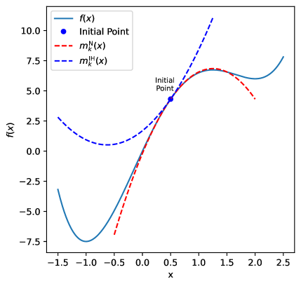
Figure 1: Graphical illustration of $f(\mathbf{x}),\ m_{k}^{N}(\mathbf{x})\ \text{and}\ m_{k}^{IH}(\mathbf{x})$

Computing $\alpha$ exactly over an interval using Eq. 3.8 is equivalent to solving a nonconvex optimization problem to global optimality, which could be more difficult than solving Eq. 1.1. Therefore, an efficient and scalable alternative is needed to obtain a reliable lower bound on the minimum eigenvalue over the interval. In the following subsection, we introduce the concept of the interval Hessian [47] and explain how it can be leveraged to compute a bound on the minimum eigenvalue over an interval in a computationally tractable manner.

3.2 Interval Hessian

We adopt an interval-based Hessian approximation strategy to overcome the computational challenges associated with estimating $\alpha$ using Eq. 3.8. Specifically, we replace the exact variable-dependent Hessian ($\nabla^{2}\mathcal{L}(\mathbf{x})$) with an interval Hessian matrix ($[\nabla^{2}\mathcal{L}(\mathbf{x}]$) computed using interval arithmetic such that $\nabla^{2}\mathcal{L}(\mathbf{x})\subseteq[\nabla^{2}\mathcal{L}(\mathbf{x}],\forall\mathbf{x}\in[\mathbf{x}^{L},\mathbf{x}^{U}]$. Such a strategy offers considerable scalability and computational advantages.

This interval Hessian strategy introduces a fundamental trade-off: the accuracy of the Hessian approximation versus computational cost. Specifically, using intervals naturally leads to conservativeness—looser intervals yield less accurate Hessian approximation (Theorem 1) and thus potentially less effective search directions. Conversely, tighter intervals reduce this conservativeness, but require increased computational effort because the Hessian needs to be recomputed and the linear equation (Eq. 3.4) resolved to find the search direction if the iterate $\mathbf{x}_{k}\notin[\mathbf{x}^{L},\mathbf{x}^{U}]$ because $||\nabla^{2}L(\mathbf{x}_{k-1})-\nabla^{2}f(\mathbf{x}_{k})||$ may not be bounded.

3.2.1 Interval Hessian Illustrative example

We illustrate interval Hessian computation using the following problem:

$$f({x}_{1},{x}_{2})=\left(1.5-{x}_{1}(1-{x}_{2})\right)^{2}+\left(2.25-{x}_{1}(1-{x}_{2}^{2})\right)^{2}+\left(2.625-{x}_{1}(1-{x}_{2}^{3})\right)^{2}$$ (3.15)

$$0\leq{x}_{1},{x}_{2}\leq 2$$

Then, the Hessian is:

$${\nabla^{2}f(x_{1},x_{2})}=\begin{pmatrix}\frac{\partial^{2}f}{\partial{x}_{1}^{2}}&\frac{\partial^{2}f}{\partial{x}_{1}\partial{x}_{2}}\\ \frac{\partial^{2}f}{\partial{x}_{2}\partial{x}_{1}}&\frac{\partial^{2}f}{\partial{x}_{2}^{2}}\end{pmatrix}$$

where:

$$\frac{\partial^{2}f}{\partial{x}_{1}^{2}} =2(1-{x}_{2})^{2}+2(1-{x}_{2}^{2})^{2}+2(1-{x}_{2}^{3})^{2}$$

$$\frac{\partial^{2}f}{\partial{x}_{2}^{2}} ={x}_{1}\left(30{x}_{1}{x}_{2}^{4}+12{x}_{1}{x}_{2}^{2}-12{x}_{1}{x}_{2}-2{x}_{1}+31.5{x}_{2}+9\right)$$

$$\frac{\partial^{2}f}{\partial{x}_{1}\partial{x}_{2}} =2{x}_{1}{x}_{2}^{5}+8{x}_{1}{x}_{2}^{3}-2{x}_{1}{x}_{2}^{2}-4{x}_{1}{x}_{2}-4{x}_{1}+575{x}_{2}^{2}+9{x}_{2}+3$$

We perform interval arithmetic using the Gaol package [28] to obtain the following interval Hessian.

$$\nabla^{2}f({x}_{1},{x}_{2})\subseteq[\nabla^{2}f({x}_{1},{x}_{2})]=\begin{pmatrix}[0,118]&[-69,860]\\ [-69,860]&[0,2152]\end{pmatrix}$$ (3.16)

for $0\leq{x}_{1},{x}_{2}\leq 2$. We also compute the interval Hessian by global minimization and maximization of each Hessian element using Gurobi and obtain the following:

$$[\nabla^{2}f({x}_{1},{x}_{2})]^{*}=\begin{pmatrix}[0,118]&[-5,860]\\ [-5,860]&[0,2152]\end{pmatrix}$$ (3.17)

For this function, Gurobi-based optimization took approximately 47.1 milliseconds. In contrast, the interval arithmetic approach computed the bounds in roughly 0.0497 milliseconds, offering significantly faster but conservative bounds. Once the interval Hessian is computed, we estimate the minimum eigenvalue of the interval Hessian by using the following equation:

$$\alpha\geq\max\left\{{0,-\frac{1}{2}\lambda_{min}([\nabla^{2}f])}\right\}$$ (3.18)

where $\lambda_{min}$ is the minimum eigenvalue of the interval Hessian. Next, we discuss various methods to compute the minimum eigenvalue of an interval matrix.

3.3 $\mathbf{\alpha}$ Calculation methods

3.3.1 Approximate Gerschgorin theorem (GGN) for interval matrices

This technique is based on applying the Gerschgorin theorem [3] on an interval matrix. For a real interval matrix $[\mathbf{A}]=([\underaccent{\bar}{a}_{ij},\bar{a}_{ij}])$, the lower bound on the minimum eigenvalues is as follows:

$$\lambda_{min}([\mathbf{A}])\geq\min_{i}\bigg[\underaccent{\bar}{a}_{ii}-\sum_{j\neq i}\max(|\underaccent{\bar}{a}_{ij}|,|\bar{a}_{ij}|)\bigg]$$ (3.19)

The computational complexity of this method is $\mathcal{O}(n^{2})$. We use the non-linear two-variable function given in Eq. 3.15 to illustrate the use of Eq. 3.19. Using the interval Hessian in Eq. 3.16 and 3.17, we estimate $\lambda_{min}$ to be $-860$ and $-860$, respectively.

3.3.2 E-Matrix (EM) Method

This method is an extension of the theorems developed by Deif [21] and Rohn [59] for the calculation of the lower bound on minimum eigenvalue $\lambda_{min}([\mathbf{A}])$ for a real interval matrix $[\mathbf{A}]$.

$$\lambda_{min}(\mathbf{[A]})\geq\lambda_{min}(\widetilde{\mathbf{A}}_{M}+\mathbf{E})-\rho(\widetilde{\Delta\mathbf{A}}+|\mathbf{E}|)$$ (3.20)

where, radius matrix $\Delta\mathbf{A}=(\Delta a_{ij})$ and $\Delta a_{ij}=\dfrac{\overline{a}_{ij}-\underline{a}_{ij}}{2}$, modified radius matrix $\widetilde{\Delta\mathbf{A}}=(\widetilde{\Delta a}_{ij})$ and

$$\widetilde{\Delta a}_{ij}=\begin{dcases}0&\text{if }i=j,\\ \Delta a_{ij}&\text{otherwise}\end{dcases}$$

Mid-point matrix $\mathbf{A}_{M}=(a_{M,ij})$ where $a_{M,ij}=\dfrac{\overline{a}_{ij}+\underline{a}_{ij}}{2}$, modified mid-point matrix $\tilde{\mathbf{A}}_{M}=(\widetilde{a}_{M,ij})$ where

$$\widetilde{a}_{M,ij}=\begin{dcases}\underline{a}_{ij}&\text{if }i=j,\\ a_{M,ij}&\text{otherwise}\end{dcases}$$

where $\mathbf{E}$ is an arbitrary matrix that is taken to be equal to $\Delta\mathbf{A}$. The computational complexity of this method is $\mathcal{O}(n^{3})$. We use the non-linear two-variable function given in Eq. 3.15 to illustrate the use of Eq. 3.20. Using the interval Hessian in Eqs. 3.16 and 3.17, we estimate $\lambda_{min}$ to be $-1332.92$ and $-1331.88$, respectively.

3.3.3 Mori-Kokame (MK) Method

This method is an extension of the theorems developed by Mori and Kokame (MK) [49], which suggest using lower and upper bound matrices to calculate the lower bound on the minimum eigenvalue for the interval matrix.

$$\lambda_{min}([\mathbf{A}])\geq\lambda_{min}(\underline{\mathbf{A}})-\rho(\overline{\mathbf{A}}-\underline{\mathbf{A}})$$ (3.21)

where $\overline{\mathbf{A}}=(\overline{a}_{ij})$ and $\underline{\mathbf{A}}=(\underline{a}_{ij})$. The computational complexity of this method is $\mathcal{O}(n^{3})$. We use the non-linear two-variable function given in Eq. 3.15 to illustrate the use of Eq. 3.21. Using the interval Hessian in Eqs. 3.16 and 3.17, we estimate $\lambda_{min}$ to be $-2581.44$ and $-2475.11$, respectively. For this example, we observed that the GGN method, which is the least computationally expensive method, provides the tightest $\lambda_{min}$. However, this may not be always the case.

3.4 Algorithm Structure

We incorporate the proposed search direction in a line-search framework and develop INTHOP - INTerval Hessian-based OPtimization. In this section, we present two variants of INTHOP based on fixed and adaptive interval size selection, represented as INTHOP:F and INTHOP:A, respectively.

3.4.1 INTHOP:F

The line search framework finds the next iterate $\mathbf{x}_{k+1}$ based on the search direction $\mathbf{p}_{k}$ and the step length $\theta_{k}$:

$$\mathbf{x}_{k+1}=\mathbf{x}_{k}+\theta_{k}\mathbf{p}_{k}$$ (3.22)

The INTHOP algorithm with fixed interval size, denoted as INTHOP:F, is given in Algorithm 1. We select two iteration counts, $t$ and $k$. The former functions as the outside iteration counter, while the latter serves as the inner iteration counter. The iteration counter $t$ is updated when the Hessian is computed. In contrast, $k$ is updated whenever a new iterate is generated. At the beginning of iteration $k$, we check whether the gradient norm is less than the pre-defined tolerance or if the number of iterations has exceeded. If either of the conditions is satisfied, we terminate and return the solution. Otherwise, we check whether the current iterate $\mathbf{x}_{k}$ lies in the interval $[\mathbf{x}_{t}^{L},\mathbf{x}_{t}^{U}]$.

Hessian modification becomes essential whenever the current iterate $\mathbf{x}_{k}$ exits the interval around which the previous Hessian was computed because the difference between $\nabla^{2}\mathcal{L}_{t}$ and $\nabla^{2}{f}_{k}$ may not be bounded. At such points, we establish a new interval of length $\delta$ centered at $\mathbf{x}_{t}$, and compute the interval Hessian within this region. This localized approximation captures the curvature of the objective function over the updated interval and informs the subsequent search directions. One approach to construct intervals is to expand the interval around the current iterate symmetrically, as given in Algorithm 2.

Once the interval is constructed, the interval Hessian and the corresponding $\alpha$ are calculated using one of the methods outlined in Section 3.3. Thereafter, we compute $\nabla^{2}L_{t}$, its inverse, and the search direction. The search direction $\mathbf{p}_{k}$ (Eq. 3.4) fulfills ($\mathbf{g}_{k}^{\top}\mathbf{p}_{k}$), ensuring a reduction in the function value. Consequently, $f_{k+1}<f_{k}$ after each iteration. The step length is found by backtracking line search, given in Algorithm 4, such that the Armijo condition is satisfied. The new iterate is then obtained by taking a step length $\theta_{k}$ in the direction $\mathbf{p}_{k}$ from the current iterate $x_{k}$. The procedure is repeated until a convergence criterion is satisfied.

Figure 2 demonstrates the iterative mechanics of our algorithm with the bounds updating scheme given in Algorithm 2 using a one-dimensional function. The figure shows that a new interval of length $\delta$, centered around the current iterate, represented by the square markers, is created. The new interval is created at the starting point or when the current iterate $\mathbf{x}_{k}\notin[\mathbf{x}_{t}^{L},\mathbf{x}_{t}^{U}]$. At these points, the expensive computations occur. First, the interval Hessian is computed. Second, the lower bound on the minimum eigenvalue for the interval Hessian is estimated, and the Hessian matrix is modified to ensure positive definiteness. Third, the modified Hessian matrix is inverted to compute the search direction. Circle markers represent points where $\mathbf{x}_{k}\in[\mathbf{x}_{t}^{L},\mathbf{x}_{t}^{U}]$. In these cases, only the gradient is evaluated, and the search direction is computed by multiplying the stored inverse Hessian from the $t^{\text{th}}$ iteration by the gradient vector.

Algorithm 1 INTHOP:F

Init. Choose $\mathbf{x}_{0}\in\mathbb{R}^{n},\ \epsilon_{g}\in(0,1),\ t=0;$

for $k=0,1,2,\dots$ do

  if $\|\mathbf{g}_{k}\|<\epsilon_{g}$ then

   Terminate - Solution found;   end if

  if $k>iter_{max}$ then

   Terminate   end if

  if $k=0$ or $\mathbf{x}_{k}\notin[\mathbf{x}_{t}^{L},\mathbf{x}_{t}^{U}]$ then

   $t\xleftarrow{}t+1$

   Go to Algorithm 2 to compute $\mathbf{x}^{L}_{t}$ and $\mathbf{x}^{U}_{t}$

   Go to Algorithm 3 to compute $\nabla^{2}\mathcal{L}_{t}$

   Compute $\nabla^{2}\mathcal{L}_{t}^{-1}$   end if

  Find the search direction by solving

$$\mathbf{p}_{k}=-\nabla^{2}\mathcal{L}_{t}^{-1}\mathbf{g}_{k}$$ (3.23)

  Compute step length $\theta_{k}$ using Algorithm 4 and set $\mathbf{x}_{k+1}=\mathbf{x}_{k}+\theta_{k}\mathbf{p}_{k}$ end for

Algorithm 2 Symmetric interval generation scheme

Init. $\delta\in\mathbb{R}^{+}$

for $i=0,1,2,\dots,n$ do

  $\mathbf{x}^{L}_{t,i}=\mathbf{x}_{k,i}-\delta/2$

  $\mathbf{x}^{U}_{t,i}=\mathbf{x}_{k,i}+\delta/2$ end for

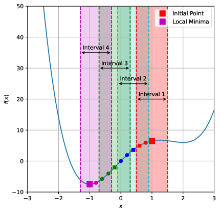
Figure 2: Graphical illustration of INTHOP with fixed interval size (INTHOP:F) and Algorithm 2 used to generate intervals.

Algorithm 3 Hessian approximation algorithm

Compute the Interval Hessian $[\nabla^{2}f(\mathbf{x})]$ for $\mathbf{x}\in[\mathbf{x}_{t}^{L},\mathbf{x}_{t}^{U}]$ using interval arithmetic

Compute $\lambda_{t,min}$ using Equation 3.19, 3.20 or 3.21

$$\alpha=\min\left(0,-\frac{1}{2}\lambda_{t,min}\right)$$ (3.24)

Compute the positive-definite Hessian approximation,

$$\nabla^{2}\mathcal{L}_{t}=\nabla^{2}f_{t}+2\alpha\mathbf{I}$$ (3.25)

Algorithm 4 Backtracking line search

Choose $\theta_{0}>0,c_{1}\in(0,1),\rho\in(0,1)$
$\theta\leftarrow\theta_{0}$

while $f(\mathbf{x}_{k}+\theta\mathbf{p}_{k})>f(\mathbf{x}_{k})+c_{1}\theta\nabla f(\mathbf{x}_{k})^{\top}\mathbf{p}_{k}$ do

  $\theta\leftarrow\rho\theta$

end while
$\theta_{k}\leftarrow\theta$
$\mathbf{x}_{k+1}\leftarrow\mathbf{x}_{k}+\theta_{k}\mathbf{p}_{k}$

3.4.2 INTHOP:A

INTHOP:F (Algorithm 1) assumed a constant value of the interval size, making it a hyperparameter for our algorithm. However, the same value of interval size might not be appropriate for a different function or different regions of a function. Accordingly, we develop two variants of INTHOP based on adaptive interval size. Theorem 1 stated the effect of interval size on the difference between $\nabla^{2}L_{t}$ and $\nabla^{2}f_{k}$. Now, we formally state the effect of the regularization parameter $\alpha$ on the norm of the computed search direction.

Lemma 1.

Let the search direction be given by $\mathbf{p}_{k}=-\nabla^{2}\mathcal{L}_{t}^{-1}\nabla f_{k}$, where $\nabla^{2}\mathcal{L}_{t}=\nabla^{2}f_{t}+2\alpha\mathbf{I}$. Then, the norm of the $\mathbf{p}_{k}$ at iteration $k$ satisfies:

$$\|\mathbf{p}_{k}\|\leq\frac{\|\nabla f_{k}\|}{\lambda_{\min}(\nabla^{2}f_{t})+2\alpha}.$$ (3.26)

Proof.

Refer A. ∎

A high $\alpha$ value ensures that $\nabla^{2}L_{t}$ is positive definite and, consequently, the search direction is descent. However, it leads to conservative steps and potentially slow convergence. Therefore, an appropriate balance is required to ensure positive definiteness and step lengths. We develop two INTHOP variants based on adaptively updating the interval size.

3.4.3 INTHOP:A1

This method is based on the observation that the magnitude of the search direction can serve as an indicator of the quality of the Hessian approximation. Specifically, a small search direction norm may imply that the algorithm is approaching a stationary point (small gradient norm) or that $\alpha$ is too large due to a large interval size. Conversely, a large search direction indicates that the interval is sufficiently small and the Hessian approximation is reliable.

To quantify this, we define the following ratio:

$$\eta_{t}=\frac{r}{\sqrt{n}}\times\frac{\|\mathbf{p}_{k-1}\|_{1}}{\sqrt{\|\mathbf{p}_{k-1}\|_{2}^{2}+\beta}}$$ (3.27)

where $\beta>0$ is a small regularization constant to avoid division by zero and dampening the ratio $\eta_{t}$. The parameter $r$ is a scaling factor that adjusts the interval size. This ratio $\eta_{t}$ is inspired by the adaptive learning rate strategies used by machine learning optimizers such as Adam [34]. These methods combine first- and second-moment estimates of the gradients to modulate the step size adaptively to improve convergence rates. Adam, for instance, adjusts the step size by dividing the running average of the gradient (first moment) by the square root of the running average of the squared gradient (second moment) with a small constant added to prevent division by zero. This dampening term ($\beta$) also smooths the update to prevent instability from sudden gradient spikes.

For any non-zero vector $\mathbf{p}_{k}\in\mathbb{R}^{n}$, the ratio is bounded as:

$$0\leq\eta_{t}\leq r\frac{\|\mathbf{p}_{k-1}\|_{1}}{\sqrt{\|\mathbf{p}_{k-1}\|_{2}^{2}+\beta}}$$ (3.28)

In the regime where $\|\mathbf{p}_{k}\|_{2}^{2}\gg\beta$, the upper bound asymptotically approaches r. When the search direction is small in magnitude, the ratio $\eta_{t}$ is small, indicating potential over-regularization and suggesting a reduction in the interval size. Conversely, a higher $\eta_{t}$ suggests that the current interval size is effective, and it can be increased to allow larger steps. The INTHOP variant with adaptive interval size based on Eq. 3.27 is denoted as INTHOP:A1 and summarized in Algorithm 5.

Algorithm 5 INTHOP:A1

Init. Choose $\mathbf{x}_{0}\in\mathbb{R}^{n},\ \epsilon_{g}\in(0,1),\ \delta=\delta_{0},\ r>0,\ \beta>0,\ t=0;$

for $k=0,1,2,\dots$ do

  if $\|\mathbf{g}_{k}\|<\epsilon_{g}$ then

   Terminate - Solution found;   end if

  if $k>iter_{max}$ then

   Terminate   end if

  if $k=0$ or $\mathbf{x}_{k}\notin[\mathbf{x}_{t}^{L},\mathbf{x}_{t}^{U}]$ then

   if $k=0$ then

     $\delta_{t}=\delta_{0}$

   else

     Update $\delta_{t}$

$$\eta_{t}=\frac{r}{\sqrt{n}}\times\frac{\|\mathbf{p}_{k-1}\|_{1}}{\sqrt{\|\mathbf{p}_{k-1}\|_{2}^{2}+\beta}}$$ (3.29)

$$\delta_{t}=\delta_{t-1}\times\eta_{t}$$ (3.30)

   end if

   $t\xleftarrow{}t+1$

   Go to Algorithm 2 to compute $\mathbf{x}^{L}_{t}$ and $\mathbf{x}^{U}_{t}$

   Go to Algorithm 3 to compute $\nabla^{2}\mathcal{L}_{t}$

   Compute $\nabla^{2}\mathcal{L}_{t}^{-1}$   end if

  Find the search direction by solving

$$\mathbf{p}_{k}=-\nabla^{2}\mathcal{L}_{t}^{-1}\mathbf{g}_{k}$$ (3.31)

  Compute step length $\theta_{k}$ using Algorithm 4 and set $\mathbf{x}_{k+1}=\mathbf{x}_{k}+\theta_{k}\mathbf{p}_{k}$ end for

3.4.4 INTHOP:A2

We created a modified second-order Taylor model (Equation 3.3) to obtain the search direction within a given interval. INTHOP algorithm can also be interpreted through the lens of the trust-region method as follows. From the $t^{\text{th}}$ to the $(t+1)^{\text{th}}$ iterate, we move within a fixed-size interval constructed around the iterate $\mathbf{x}_{t}$. Once an iterate reaches any boundary of this interval, a new interval is formed. This behavior is similar to classical trust-region methods, where, for a given local model, we define a region within which we trust the model to approximate the objective function. The size of this region is important. If it is too small, the model may be accurate, but progress is slow; if it is too large, the model (Eq. 3.3) may not accurately represent the true function. In trust-region methods, a ratio is computed between the actual reduction and the predicted reduction (i.e., the decrease predicted by the local model), and this ratio is used to adjust the trust-region size accordingly.

In our case, we update the interval size based on the performance of the algorithm in the previous interval. We define the ratio $\xi_{t}$ here as follows:

$$\xi_{t}=\frac{f(\mathbf{x}_{t})-f(\mathbf{x}_{t+1})}{-(\mathbf{g}_{t}^{\top}\mathbf{s}_{t}+\mathbf{s}_{t}^{\top}\nabla^{2}\mathcal{L}_{t}\mathbf{s}_{t})}$$ (3.32)

where, $\mathbf{s}_{t}=\mathbf{x}_{t+1}-\mathbf{x}_{t}$. Here, the numerator is the decrease in the actual function value in the last interval, and the denominator shows the decrease obtained by the model. The following three cases may arise: (1) if $\eta_{t}<0$, then the objective function increases while the model predicted it to decrease, which means the previous value of the interval size gave an inaccurate representation of the objective function. (2) If $\eta_{t}$ is close to zero and positive, then the model has significantly overestimated the decrease in the objective function. (3) If $\eta_{t}$ is close to 1, the model’s predicted decrease closely matches the actual decrease in the objective function. In the first two cases, the interval size is reduced to improve the accuracy of the Hessian approximation. For the third case, the current interval size is retained or increased depending on the value of $\eta_{t}$. The INTHOP variant based on Eq. 3.32 to update the interval size is given in Algorithm 6.

Algorithm 6 INTHOP:A2

Init. Choose $\mathbf{x}_{0}\in\mathbb{R}^{n},\ \epsilon_{g}\in(0,1),\ \delta=\delta_{0},\ iter_{max}>0,\ \delta_{max}>\delta_{min}>0,\ t=0;$

for $k=0,1,2,\dots$ do

  if $\|\mathbf{g}_{k}\|<\epsilon_{g}$ then

   Terminate - Solution found;   end if

  if $k>iter_{max}$ then

   Terminate   end if

  if $k=0$ or $\mathbf{x}_{k}\notin[\mathbf{x}_{t}^{L},\mathbf{x}_{t}^{U}]$ then

   if $k=0$ then

     $\delta_{t}=\delta_{0}$

   else

     $t\xleftarrow{}t+1$

     Compute $\eta_{t}$

$$\xi_{t}=\frac{f(\mathbf{x}_{t})-f(\mathbf{x}_{t+1})}{-(\mathbf{g}_{t}^{\top}\mathbf{s}_{t}+\mathbf{s}_{t}^{\top}\nabla^{2}\mathcal{L}_{t}\mathbf{s}_{t})}$$ (3.33)

     if $\xi_{t}<\frac{1}{4}$ then

      $\delta_{t}\leftarrow\max\left(\frac{\delta_{t-1}}{2},\delta_{\min}\right)$

     else if $\xi_{t}>\frac{3}{4}$ then

      $\delta_{t}\leftarrow\min(4\cdot\delta_{t-1},\delta_{\max})$

     else if $\frac{1}{4}\leq\xi_{t}\leq\frac{3}{4}$ then

      $\delta_{t}\leftarrow\delta_{t-1}$      end if    end if

   Go to Algorithm 2 to compute $\mathbf{x}^{L}_{t}$ and $\mathbf{x}^{U}_{t}$

   Go to Algorithm 3 to compute $\nabla^{2}\mathcal{L}_{t}$

   Compute $\nabla^{2}\mathcal{L}_{t}^{-1}$   end if

  Find the search direction by solving

$$\mathbf{p}_{k}=-\nabla^{2}\mathcal{L}_{t}^{-1}\mathbf{g}_{k}$$ (3.34)

  Compute step length $\theta_{k}$ using Algorithm 4 and set $\mathbf{x}_{k+1}=\mathbf{x}_{k}+\theta_{k}\mathbf{p}_{k}$ end for

4 Competing Algorithms

In this section, we describe several widely used optimization algorithms: the steepest descent, quasi-Newton, and Newton’s methods. The steepest descent and quasi-Newton methods are classical optimization algorithms whose details can be found in standard optimization textbooks such as [53]. Specifically, we implement the BFGS algorithm as the quasi-Newton method. Newton’s method finds the search direction at each iteration $k$, denoted as $\mathbf{p}_{k}^{N}$, by using the following equation:

$$\mathbf{p}_{k}^{N}=-(\nabla^{2}f(\mathbf{x}_{k}))^{-1}\nabla f(\mathbf{x}_{k})$$ (4.1)

Computing this search direction at each iteration requires $\mathcal{O}(n^{3})$ operations due to the Hessian inversion or matrix factorization. Suppose the Hessian is positive definite at the current iterate $\mathbf{x}_{k}$. In that case, the resulting search direction is guaranteed to be a descent direction. However, if the Hessian is indefinite, direct application of Newton’s method may fail or lead to non-descent steps. Therefore, the Hessian matrix needs to be updated so that it is positive semidefinite.

A simple strategy to address indefiniteness involves adjusting the Hessian by introducing a parameter $\tau>0$ chosen such that the modified Hessian, $\nabla^{2}f(\mathbf{x}_{k})+\tau\mathbf{I}$, becomes positive definite. Algorithm 7 illustrates one approach, where the value of $\tau$ is incrementally increased until positive definiteness is ensured. Positive definiteness is verified using Cholesky decomposition, which requires $\mathcal{O}(n^{3})$ operations. Thus, whenever non-convexity is encountered, it may take multiple $\mathcal{O}(n^{3})$ operations to find an appropriate value of $\tau$ such that it is positive definite. The approach with Newton’s method with Algorithm 7 is referred to as Newton-CAMI. Although there are other effective strategies to modify the Hessian, the approach given in Algorithm 7 ensures accurate Hessian approximation, allowing us to explore trade-offs between Hessian approximation and computational expense associated with ensuring accurate Hessian.

Algorithm 7 Cholesky with Added Multiple of Identity(CAMI)

Init. Choose $\tau_{0}=0$

for $i=0,1,2,\dots$ do

  Cholesky Factorization: $LL^{T}=\nabla^{2}f_{k}+\tau_{i}\mathbf{I}_{n}$

  if factorization is completed successfully then

   Terminate

  else

   $\tau_{i+1}\leftarrow\tau_{i}+1$   end if end for

5 Numerical Results

INTHOP is implemented in C++. All computational runs were performed on a PC with a 12th Gen Intel Core i7-12700 processor (12 cores, 2.10 GHz) and 32 GB RAM. We used the Gaol library [28] to perform interval arithmetic operations. We employed the Eigen library for linear algebra operations, including Cholesky decomposition and inverse computation [30]. Symbolic function representation and the computation of gradients and Hessians have been implemented using the GiNaC library [12], which allows for symbolic differentiation in C++. We have used the following parameters while implementing the above algorithms: gradient tolerance $\epsilon_{g}=0.001$, maximum number of iterations $iter_{\max}=10000$, backtracking factor $\rho=0.5$, Armijo condition constant $c_{1}=0.001$, initial Armijo step length $\theta_{0}=1$, regularization parameter for INTHOP:A1 $\beta=1$, initial interval size $\delta_{0}=0.1$, and the interval scaling factor $r=2$.

In this section, we apply the INTHOP algorithm on a few illustrative examples and on an extensive set of problems as referenced in [56]. The complete problem set and the initial guess for each problem are given in ESI. These experiments evaluate the performance of the INTHOP variants compared to other algorithms. Specifically, we assess the convergence properties and computational efficiency of our method across the problem set, highlighting the advantages and trade-offs compared to the traditional point-based methods.

5.1 Illustrative Examples

5.1.1 Example 1

The objective function considered is given by:

$$f({x}_{1},{x}_{2})=\sum_{j=1}^{17}\sum_{k=1}^{m_{j}}\left(t_{j,k}-\left[\exp(-2j{x}_{2})(0.49-{x}_{1})+{x}_{1}\right]\right)^{2}$$ (5.1)

where $m_{j}$ represents the number of groups at index $j$ and $t_{j,k}$ is a constant. Figure 3 illustrates the paths followed by iterates produced by the steepest descent method, quasi-newton BFGS, and INTHOP:F with $\delta=0.1$ employing three $\alpha$ calculation methods detailed in Section 3.3. The BFGS approach followed a path similar to the steepest descent but could not find a descent direction after nine iterations. The quasi-Newton approach may fail to locate a descent direction for nonconvex problems when the Armijo condition is applied to determine the step size $\theta$ (refer to chapter 6 of [53]). We observe that steepest descent tends to stagnate in regions characterized by small gradient magnitudes and fails to reach a local minimum within 10,000 iterations. Conversely, INTHOP:F with the three $\alpha$ calculations methods follow nearly identical paths and converge to the same local solution. Specifically, the Gerschgorin-based(GGN) method achieves convergence in 442 iterations, requiring 8 Hessian evaluations and 8 $\mathcal{O}(n^{3})$ operations. The EM method converges in 265 iterations, using 7 Hessian evaluations and 14 $\mathcal{O}(n^{3})$ operations, while the MK method requires 1041 iterations, involving 9 Hessian evaluations and 18 $\mathcal{O}(n^{3})$ operations.

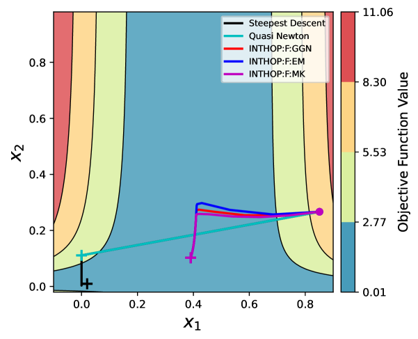
Figure 3: Paths taken by steepest descent, quasi-Newton, and INTHOP:F on illustrative example 1.

5.1.2 Example 2

We minimize an objective function defined as:

$$f({x}_{1},{x}_{2})=C_{A}{x}_{1}+C_{B}{x}_{2}+C_{C}-\left\{\sum_{(i,j)\in S}C_{ij}{x}_{1}^{i}{x}_{2}^{j}+\frac{C_{D}}{1+{x}_{2}}+C_{E}e^{C_{F}{x}_{1}{x}_{2}}\right\}$$ (5.2)

where $C_{A},\dots,C_{F}$ and $C_{ij}$ are constants. Figure 4(a) illustrates the paths traced by iterates generated by Newton-CAMI and three INTHOP variants corresponding to the different methods for calculating $\alpha$, as detailed in Section 3.3. To emphasize the computational burden of $\mathcal{O}(n^{3})$ operations, we intentionally added a 1-second delay using the sleep function whenever such operations were performed. Figure 4(b) highlights that all INTHOP variants converge to better solutions faster than Newton-CAMI for this problem.

For INTHOP:F:GGN, we use $\delta=1$; for EM and MK, we use 0.1 and 0.5, respectively, as these values yield the best performance in each case. Newton-CAMI performs 7 Hessian inversions and 3 Cholesky decompositions, while MK and EM perform 3 inversions and 3 modifications. In contrast, GGN performs only 3 matrix inversions, with Hessian modifications that require $\mathcal{O}(n^{2})$ operations. This difference in computational cost is clearly reflected in Figure 4(b), where Newton-CAMI shows the highest expense and GGN the lowest.

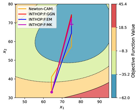
(a)

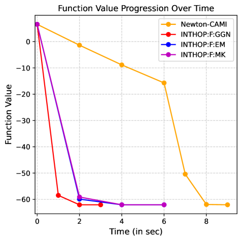
(b)

Figure 4: (A) Comparison of paths take by INTHOP:F and NEWTON:CAMI on illustrative example 2. (B) Function value as a function of time for INTHOP:F and NEWTON:CAMI.

5.2 Benchmarking Interval Hessian Frameworks

In this section, we utilize data profiles [48] to systematically benchmark the effectiveness of the optimization algorithm and investigate the effects of various factors on its performance. These profiles facilitate structured comparisons by explicitly defining three fundamental elements: a set of benchmark optimization problems, denoted by $\mathcal{S}$; a collection of optimization algorithms, denoted by $\mathcal{A}$; and an established convergence criterion, $\mathcal{T}$.

A data profile quantifies the absolute performance of an optimization algorithm. For each pair consisting of a problem $s\in\mathcal{S}$ and an algorithm $a\in\mathcal{A}$, we define a performance metric $m_{s,a}$, which, for example, could be the number of Hessian evaluations required to achieve the convergence criterion. Formally, the data profile $d_{a}(\zeta)$ of an algorithm $a$ indicates the proportion of benchmark problems that algorithm $a$ solves within a specified computational threshold $\zeta$. Specifically, it is given by:

$$d_{a}(\zeta)=\frac{1}{|\mathcal{S}|}\text{size}\{s\in\mathcal{S}:m_{s,a}\leq\zeta\}$$ (5.3)

where $|\mathcal{S}|$ denotes the total number of benchmark problems considered. When $m_{s,a}=\infty$, the algorithm fails to satisfy the convergence criterion for problem $s$. A problem is considered solved if and only if the final point returned by an algorithm satisfies the following conditions: $\|\mathbf{g}_{k}\|<\epsilon_{g}$ and $\lambda_{min}(\mathbf{H}_{k})>-\epsilon_{H}$, where $\epsilon_{g},\epsilon_{H}>0$. Data profiles are particularly valuable when a fixed computational budget is available, guiding the selection of algorithms most capable of solving a problem within the allocated computational budget.

5.2.1 Effect of Interval Size

A critical parameter that impacts the performance of INTHOP:F is the interval size $\delta$. A larger interval size can reduce the computational effort required for repeated Hessian evaluations and matrix inversion, but might lead to conservative steps (Lemma 1). Conversely, smaller intervals offer accuracy in capturing curvature details but incur higher computational costs due to repeated Hessian evaluations. Additionally, the accuracy of $\alpha$ depends significantly on the specific estimation method used. Our observations indicate that the MK and EM methods provide tighter $\alpha$ than the Gerschgorin method. However, the former two methods require $\mathcal{O}(n^{3})$ operations, while the Gerschgorin method requires $\mathcal{O}(n^{2})$ operations. To systematically investigate these trade-offs, we evaluate nine algorithmic variants, combining three distinct $\delta$ values (0.1, 0.5, 1) with the three $\alpha$ estimation methods discussed in Section 3.3.

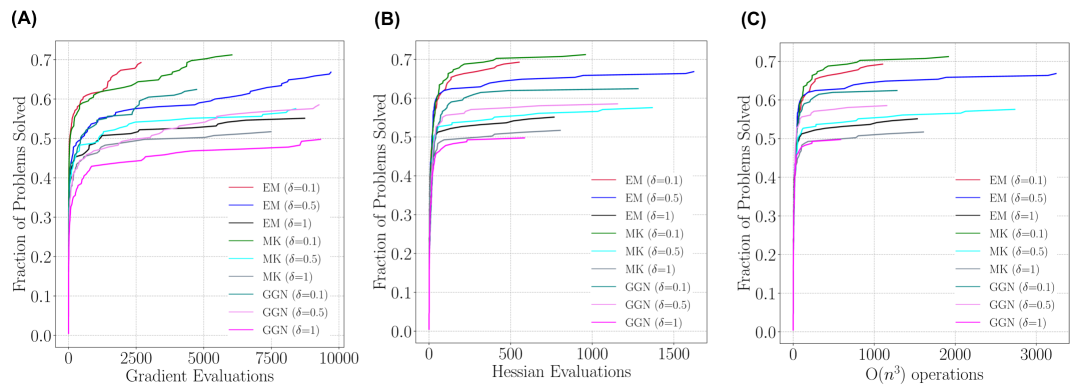
Figure 5: Fraction of problems solved by INTHOP:F variants with (A) gradient evaluations, (B) Hessian evaluations, (C) $\mathcal{O}(n^{3})$ operations

.

These variants are tested across a comprehensive benchmark set comprising 209 optimization problems taken from [56]. While the problem set consisted of bound-constrained problems, we solved them considering as unconstrained problems. The computational results are depicted in Figure 5, which shows the fraction of problems solved with the number of gradient and Hessian evaluations and $\mathcal{O}(n^{3})$ operations. Each INTHOP variant is denoted in the figures using the nomenclature <$\alpha$ calculation method>($\delta$=Interval size). Figure 5 demonstrates that our approach successfully solves approximately 70% of the problems within 5000 gradient evaluations, 500 Hessian evaluations, and 1000 $\mathcal{O}(n^{3})$ operations. Recall that if $\mathbf{x}_{k}\in[\mathbf{x}_{t}^{L},\mathbf{x}_{t}^{U}]$, computing the search direction requires gradient evaluation and a matrix-vector product. In contrast, if $\mathbf{x}_{k}\notin[\mathbf{x}_{t}^{L},\mathbf{x}_{t}^{U}]$, the Hessian and $\alpha$ are computed. The search direction is obtained by taking the product of $\nabla^{2}L_{t}$ inverse with gradient. Thus, contrary to the Newton method, which requires an equal number of gradient and Hessian evaluations to compute the search direction, INTHOP requires fewer Hessian evaluations than gradient evaluations. Furthermore, whenever $\mathbf{x}_{k}\notin[\mathbf{x}_{t}^{L},\mathbf{x}_{t}^{U}]$, the MK and EM methods require two $\mathcal{O}(n^{3})$ operations; one to estimate $\alpha$ and the second to compute the search direction. On the other hand, the GGN method requires one $\mathcal{O}(n^{2})$ operation to compute $\alpha$ and one $\mathcal{O}(n^{3})$ operations corresponding to computing the inverse of $\nabla^{2}L_{t}$ to obtain the search direction.

We make the following five observations. First, INTHOP employing the MK method to estimate $\alpha$ performs the best, followed by EM and Gerschgorin methods. Second, for the same $\alpha$ calculation method, increasing $\delta$ results in performance degradation across all metrics. Third, EM and MK methods with $\delta=0.1$ perform comparably across all performance metrics. Fourth, the EM method with $\delta=0.5$ performs slightly better than the Gerschgorin method with $\delta=0.1$, which in turn achieves a performance superior to the MK method with $\delta=0.5$ in all performance metrics. Fifth, MK and Gerschgorin methods with $\delta=0.5$ perform similarly in terms of gradient evaluations, but the latter method outperforms in terms of Hessian evaluations and $\mathcal{O}(n^{3})$ operations. The performance difference between the two methods is greater for $\mathcal{O}(n^{3})$ operations, as the Gerschgorin method requires $\mathcal{O}(n^{2})$ operations to compute $\alpha$, while the MK method requires $\mathcal{O}(n^{3})$ operations. Our results illustrate that accurately estimating $\alpha$ is critical for the algorithm’s performance, which depends on the calculation method of $\alpha$ and the size of the interval $\delta$.

The INTHOP algorithm employing MK method with $\delta=0.1$ could not solve 59 problems out of the set of 209 problems. For 21 problem instances, the algorithm reached the prescribed maximum iteration limit set at 10,000; for 23 problem instances, the step size became less than tolerance; for 8 problem instances, the algorithm converged to a saddle point; for 3 problems, the initial function value approached $\pm\infty$; and for 4 problems, the Hessian became a singular matrix.

5.2.2 Adaptive Delta Evaluation

In previous sections, $\delta$ was treated as a fixed hyperparameter and we observed that it significantly impacted the overall algorithmic performance. However, the optimal interval size is inherently problem-dependent and sensitive to local landscape variations. Larger intervals lead to a larger difference in the original Hessian and its approximation (Theorem 1). In comparison, smaller intervals improve tightness but incur higher computational costs due to frequent Hessian evaluations and $\mathcal{O}(n^{3})$ operations.

To address this trade-off, we employ two adaptive interval strategies, INTHOP:A1 and INTHOP:A2, outlined in Algorithms 5 and 6, respectively. These strategies dynamically adjust $\delta$ to balance the Hessian approximation accuracy with computational overhead. The interval size is constrained within $[0.001,10]$. The lower bound on $\delta$ ensures that the algorithm does not behave like a traditional point-based method, while the upper bound ensures that the Hessian approximations are not loose. To evaluate the effectiveness of these adaptive schemes, we combine INTHOP:A1 and INTHOP:A2 with each eigenvalue estimation method in Section 3.3, and compare them with the best performing INTHOP variant with fixed interval size corresponding to $\delta=0.1$, as illustrated in Figure 5. Figure 6 shows the resulting data profiles obtained for various methods. Each adaptive variant is denoted in the figures using the nomenclature <Eigenvalue Method>:<Adaptive Variant>. We make the following key observations. First, for the same $\alpha$ calculation method, the INTHOP variant with adaptive methods to select $\delta$ performs superior to the best fixed $\delta$ method. Second, A1 with MK and EM methods performs best and solves 80% of the problems. Third, EM:A1 was unable to solve 41 problems of the set of 20 9problems. For 26 problem instances, the number of iterations exceeded; 8 problems converged to the saddle point and the remaining problems had function value approaching $\pm\infty$, or the Hessian matrix became singular. Fourth, MK:A2 solves 76% of the problems, while EM:A2 solves 73% of the problems. Fifth, for the GGN method, the A1 variant performs better than A2 with respect to gradient evaluations, but achieves a similar performance with respect to the number of Hessian evaluations and $\mathcal{O}(n^{3})$ operations.

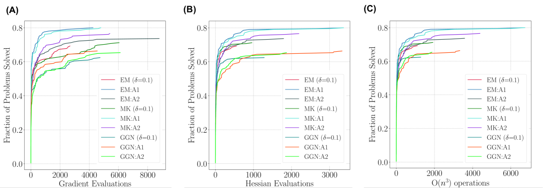
Figure 6: Data profile corresponding to fixed and adaptive $\delta$ INTHOP variants using gradient evaluations, Hessian evaluations, and $\mathcal{O}(n^{3})$ operations as the performance metrics.

Another critical question is how adaptive variants modify $\delta$ values with iterations. To illustrate this, we show the variation of $\delta$ for two problems (10_s295 and 2_gold) that were not solved by the fixed $\delta$ variant using the EM method to compute $\alpha$, while the two adaptive methods solved the two problems. The results for 10_s295 and 2_gold are shown in Figure 7 (A) and (B), respectively. The left y-axis shows the function values in blue, and the right y-axis shows $\delta$ in red with Hessian evaluations. The solid lines represent the performance of the adaptive method A1, and the dashed lines represent the A2 method. Recall that when $\textbf{x}_{t}\notin[\textbf{x}_{k}^{L},\textbf{x}_{k}^{U}]$, $\delta$ is modified and the Hessian matrix is evaluated. For 10_s295, we observe that initially $\delta$ increases for both adaptive variants to allow a larger step size during the initial phase of the algorithm. However, $\delta$ decreases to a small value as the algorithm approaches the optimal solution. For 2_gold, for EM:A1, $\delta$ strictly decreases, whereas no apparent trend is observed for EM:A2. Importantly, we note that adapting $\delta$ can achieve faster convergence.

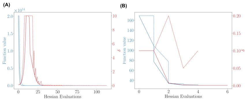
Figure 7: Variation of function value and $\delta$ with iterations for (A) 10_s295 and (B) 2_gold.

Overall, these results highlight the robustness of the adaptive interval strategies, particularly when used with the EM and MK $\alpha$ estimation methods. It consistently outperforms the fixed-interval approaches across all the performance metrics.

5.3 Comparison with Competing Algorithms

Next, we compare our proposed algorithm with Newton-CAMI (Algorithm 7), steepest descent, and quasi-Newton BFGS. For the quasi-Newton BFGS method, we select the step length $\theta$ that satisfies the Wolfe conditions. Note that we chose $\theta$ that satisfies the computationally less expensive Armijo condition for the other methods. Wolfe’s conditions are required for the quasi-Newton method to satisfy the curvature condition for nonconvex problems [53].

The data profiles are shown in Figures 8 (A), (B), (C), and (D), showing the number of function evaluations, gradient evaluations, Hessian evaluations, and $\mathcal{O}(n^{3})$ operations, respectively, required by the various methods. The steepest descent and quasi-Newton methods do not require Hessian evaluations and $\mathcal{O}(n^{3})$ operations. From these results, we draw four key conclusions. First, the algorithms using Hessian information (INTHOP and Newton-CAMI) enable solving more problems in fewer function and gradient evaluations. When comparing the fraction of problems solved based on function evaluations, we observe that the INTHOP algorithm with A1:MK and A1:EM, and Newton-CAMI solve approximately 80% of the problems within 2000 function evaluations. In contrast, the quasi-Newton and steepest descent methods underperform, struggling to solve many problems even with significantly higher function evaluations. Steepest descent, in particular, solves the fewest problems and requires the most function evaluations. This is due to two primary reasons: a larger number of iterations and repeated evaluations needed to satisfy the Armijo condition for step length ($\theta$) selection. Second, gradient evaluations reflect the number of iterations required by each algorithm. Among all the methods, only the Quasi-Newton BFGS uses Wolfe conditions for step-length selection, which can require multiple gradient and function evaluations at each iteration. Interestingly, the steepest descent begins to outperform Quasi-Newton after approximately 1000 gradient evaluations. This is likely due to BFGS requiring additional gradient evaluations to satisfy Wolfe conditions.

Third, INTHOP performs better than the Quasi-Newton method, indicating that the approximate Hessian obtained by the former method is more accurate than the latter. Fourth, Newton-CAMI solves the highest fraction of problems in all performance metrics. However, after further analysis of all the problem instances, we observed that Newton-CAMI required Hessian modifications for only 44 problems. In other words, the Hessian matrix became indefinite for 44 problem instances. These results underscore the importance of using the exact Hessian unless its modification is necessary.

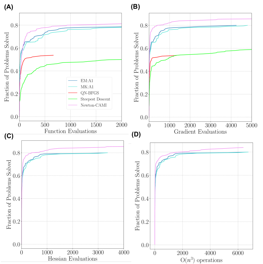
Figure 8: Fraction of problems solved by INTHOP with EM:A1 and MK:A1, steepest descent, quasi-Newton BFGS, and Newton-CAMI with (A) function evaluations, (B) gradient evaluations, (C) Hessian evaluations, and (D) $\mathcal{O}(n^{3})$ operations.

Next, we compare the performance of INTHOP and Newton-CAMI on 44 problem instances that required Hessian modifications using the latter method. Data profiles based on Hessian evaluations and $\mathcal{O}(n^{3})$ operations are shown in Figure 9 (A) and (B), respectively. We observe that while Newton-CAMI solves more problems, this comes at the cost of significantly more $\mathcal{O}(n^{3})$ operations due to repeated Cholesky decompositions required to ensure positive definiteness. Newton-CAMI modifies Hessian by incrementally increasing $\tau$, which produces more accurate Hessian approximations, but increases the total computational burden due to high $\mathcal{O}(n^{3})$ operations. In contrast, as observed in Figure 9 (B), INTHOP variants outperform Newton-CAMI by solving over 60% of the problems in 1500 $\mathcal{O}(n^{3})$ operations, and Newton-CAMI requiring over 4000 operations. These findings suggest that our algorithm can be effective for high-dimensional nonconvex problems.

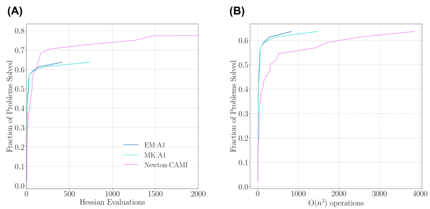
Figure 9: Fraction of problems solved by INTHOP variants and Newton-CAMI on problems requiring Hessian modifications by Newton-CAMI based on (A) Hessian evaluations and (B) $\mathcal{O}(n^{3})$ operations.

5.4 Challenging Problems

In this subsection, we present two challenging problems to highlight the potential benefits of the INTHOP algorithm. We compare the performance of the EM:A1 and MK:A1 INTHOP variants and Newton-CAMI across multiple metrics, including number of function and Hessian evaluations, $\mathcal{O}(n^{3})$ operations, and CPU time.

5.4.1 Example 1

We optimize the following function (100_s299):

$$f(\mathbf{x})=\sum_{i=1}^{99}100\left(x_{i+1}-x_{i}\right)^{2}+(1-x_{i})^{2}$$ (5.4)

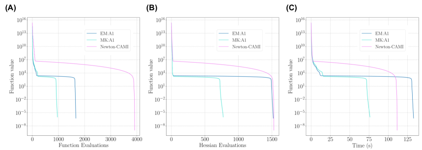
Figure 10: Function value with number of (A) function, (B) Hessian evaluations, and (C) CPU time.

The results are shown in Figure 10. Among the INTHOP variants,MK:A1 solves the problem in the least number of function and Hessian evaluations and requires the least time. Newton-CAMI requires the highest number of function evaluations but the same number of Hessian evaluations as EM:A1. Newton-CAMI requires more function evaluations to find the new iterate that satisfies the Armijo condition. Recall that the number of $\mathcal{O}(n^{3})$ operations required by the INTHOP algorithm is twice that of Hessian evaluations. On the other hand, unless the Hessian becomes indefinite, the Newton-CAMI method requires the same number of $\mathcal{O}(n^{3})$ operations as the Hessian evaluations. For this example, the Newton-CAMI algorithm did not modify the Hessian matrix because the problem is convex. Therefore, we observe that the Newton-CAMI method requires less time to find the optimal solution than the EM: A1 method. However, since the MK:A1 method requires the least number of function and Hessian evaluations and almost the same number of $\mathcal{O}(n^{3})$ operations as Newton-CAMI, it requires the least CPU time.

5.4.2 Example 2

Newton-CAMI method has the advantage that the modified Hessian is accurate; however, it can require several $\mathcal{O}(n^{3})$ operations to obtain a positive definite Hessian matrix. To illustrate this, we consider following problem (100_s305):

$$f(\mathbf{x})=\sum_{i=1}^{100}x_{i}^{2}+(\sum_{i=1}^{100}c_{i}x_{i})^{2}+(\sum_{i=1}^{100}c_{i}x_{i})^{4}$$ (5.5)

where $c_{i}$ is a constant. We show the results in Figure 11 and observe that EM:A1 and MK:A1 INTHOP variants reduce the objective function in fewer function and Hessian evaluations, and CPU time. At the third iteration, the Newton-CAMI method encounters a point at which the Hessian becomes indefinite, and even after taking $10^{6}$ $\mathcal{O}(n^{3})$ operations, the algorithm fails to find a descent direction.

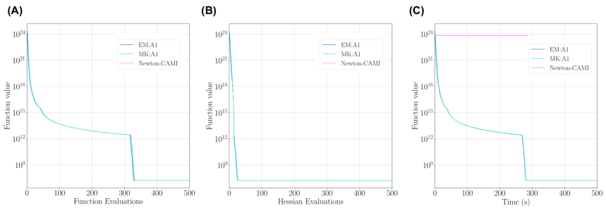
Figure 11: Function value with (A) function, (B) Hessian evaluations, and (C) CPU time.

6 Conclusion

This article introduced INTHOP, an interval Hessian-based optimization framework tailored to find a stationary point of nonconvex optimization problems. The framework is based on approximating the original Hessian such that the approximate Hessian is positive definite in an interval. The advantage of doing so is threefold. First, the search direction is guaranteed to be descent. Second, the Hessian need not be recomputed for the iterates lying within the interval. Third, the search direction can be obtained by matrix-vector product if the iterates are within the same interval. The key idea in finding a positive definite approximation of the Hessian matrix is to estimate the minimum eigenvalue of the interval Hessian matrix. The algorithm performance critically depends on the interval size and the method employed to compute the minimum eigenvalue of the interval Hessian. Accordingly, we develop INTHOP variants where the interval size remains the same, and another variant where the interval size changes with iterations. Furthermore, we implement several methods of $\mathcal{O}(n^{2})$ and $\mathcal{O}(n^{3})$ complexities to compute the minimum eigenvalue of the interval Hessian matrix. We compare the performance of INTHOP variants on a set of benchmark problems and demonstrate that INTHOP with adaptive interval size and using an $\mathcal{O}(n^{3})$ complexity method outperforms the other INTHOP variants across multiple metrics, including function, gradient, and Hessian evaluations and $\mathcal{O}(n^{3})$ operations.

We also compare the performance of INTHOP with classical point-based methods such as steepest descent, quasi-Newton BFGS, and the Newton method. We observe that INTHOP requires fewer function and gradient evaluations than steepest descent and quasi-Newton methods to find a local minimum. Since the Hessian can become indefinite for nonconvex problems, the Newton method direction is not guaranteed to be descent. Therefore, the Hessian is modified by iteratively adding a constant to the diagonal elements until it becomes positive definite. For problem instances for which the Newton method does not encounter an indefinite Hessian, we observe that the Newton method outperforms INTHOP. However, for highly nonconvex problems, we report that INTHOP requires substantially fewer $\mathcal{O}(n^{3})$ operations, illustrating its efficacy for high-dimensional nonconvex problems. A notable weakness of INTHOP is that it does not exploit the exact Hessian in convex regions of a nonconvex function, potentially missing performance gains. We aim to address this limitation in our future work.

Appendix A Proofs

This appendix provides proofs of Theorem 1 and Lemma 1 stated in Section 3.1 and 3.4.2, respectively. We prove the following results stated in Theorem 1:

• Function value bound:

  $$\left|\mathcal{L}(\mathbf{x}_{t})-f(\mathbf{x}_{k})\right|\leq\frac{L_{f}}{2}\sqrt{n}\delta+\frac{|\lambda_{min}|}{8}n\delta^{2}$$

• Gradient bound:

  $$\left\|\nabla\mathcal{L}(\mathbf{x}_{t})-\nabla f(\mathbf{x}_{k})\right\|\leq\frac{L_{g}}{2}\sqrt{n}\delta+\frac{|\lambda_{min}|}{2}\sqrt{n}\delta$$

• Hessian bound:

  $$\left\|\nabla^{2}\mathcal{L}(\mathbf{x}_{t})-\nabla^{2}f(\mathbf{x}_{k})\right\|\leq\frac{L_{H}}{2}\sqrt{n}\delta+\frac{|\lambda_{\min}|}{2}\sqrt{n}$$

Proofs of each of the above results are provided below.

Proof of function value bound: The difference between the underestimator ($\mathcal{L}$) and the true function ($f$) satisfies:

$$\left|\mathcal{L}(\mathbf{x}_{t})-f(\mathbf{x}_{k})\right| =\left|f(\mathbf{x}_{t})-f(\mathbf{x}_{k})+\sum_{i=1}^{n}\alpha(x_{i}^{L}-x_{i,t})(x_{i}^{U}-x_{i,t})\right|$$

Using triangle inequality, we get

$$\left|\mathcal{L_{f}}(\mathbf{x}_{t})-f(\mathbf{x}_{k})\right| \leq\left|f(\mathbf{x}_{t})-f(\mathbf{x}_{k})\right|+\sum_{i=1}^{n}\alpha\,|(x_{i}^{L}-x_{i,t})(x_{i}^{U}-x_{i,t})|$$

Using Eq. 3.9, the fact that the maximum of $|(x_{i}^{L}-x_{i,t})(x_{i}^{U}-x_{i,t})|$ is at $x_{i,t}=\frac{x_{i}^{U}+x_{i}^{L}}{2}$ and Eq. 3.18, we get

$$\leq L\|\mathbf{x}_{t}-\mathbf{x}_{k}\|+\sum_{i=1}^{n}\frac{|\lambda_{min}|}{8}(x_{i}^{U}-x_{i}^{L})^{2}$$

We note that $||\mathbf{x}_{t}-\mathbf{x}_{k}||\leq\sqrt{n}\frac{\delta}{2}$ and $x_{i}^{U}-x_{i}^{L}=\delta$. Using in the above equation, we get the desired result. ∎

Proof of gradient bound: Similarly, for the gradient difference, we have:

$$\left\|\nabla\mathcal{L}(\mathbf{x}_{t})-\nabla f(\mathbf{x}_{k})\right\| =||\nabla f(\mathbf{x}_{t})-\nabla f(\mathbf{x}_{k})+\alpha[2\mathbf{x}_{t}-(\mathbf{x}^{L}+\mathbf{x}^{U})]||$$

$$\leq\left\|\nabla f(\mathbf{x}_{t})-\nabla f(\mathbf{x}_{k})\right\|+|\alpha|\,\|\mathbf{x}^{L}-\mathbf{x}^{U}\|$$

$$\leq L_{g}\|\mathbf{x}_{t}-\mathbf{x}_{k}\|+|\alpha|\sqrt{n}\delta$$

$$\leq\frac{L_{g}}{2}\sqrt{n}\delta+\frac{|\lambda_{min}|}{2}\sqrt{n}\delta$$

∎

Proof of Hessian Bound: Finally, for the Hessian difference, we have:

$$\left\|\nabla^{2}\mathcal{L}(\mathbf{x}_{t})-\nabla^{2}f(\mathbf{x}_{k})\right\| =\left\|\nabla^{2}f(\mathbf{x}_{t})-\nabla^{2}f(\mathbf{x}_{k})+\alpha\mathbf{I}\right\|$$

$$\leq\left\|\nabla^{2}f(\mathbf{x}_{t})-\nabla^{2}f(\mathbf{x}_{k})\right\|+|\alpha|\sqrt{n}$$

$$\leq L_{H}\|\mathbf{x}_{t}-\mathbf{x}_{k}\|+|\alpha|\sqrt{n}$$

$$\leq\frac{L_{H}}{2}\sqrt{n}\delta+\frac{|\lambda_{\min}|}{2}\sqrt{n}$$

∎
Proof of Lemma 1

Proof.

The reciprocal of its minimum eigenvalue bounds the spectral norm of the inverse Hessian approximation:

$$\|\nabla^{2}\mathcal{L}_{t}^{-1}\|_{2}=\frac{1}{\lambda_{\min}(\nabla^{2}\mathcal{L}_{t})}$$

Since $\nabla^{2}\mathcal{L}_{t}=\nabla^{2}f(\mathbf{x}_{t})+2\alpha\mathbf{I}$, it follows that:

$$\lambda_{\min}(\nabla^{2}\mathcal{L}_{t})=\lambda_{\min}(\nabla^{2}f(\mathbf{x}_{t}))+2\alpha$$

Therefore:

$$\|\mathbf{p}_{k}\|=\|\nabla^{2}\mathcal{L}_{t}^{-1}\nabla f(\mathbf{x}_{k})\|\leq\|\nabla^{2}\mathcal{L}_{t}^{-1}\|\,\|\nabla f(\mathbf{x}_{k})\|=\frac{\|\nabla f(\mathbf{x}_{k})\|}{\lambda_{\min}(\nabla^{2}f(\mathbf{x}_{t}))+2\alpha}$$

∎

References

- [1] Adjiman, C. S., Androulakis, I. P., and Floudas, C. A. (1998a). A global optimization method, bb, for general twice-differentiable constrained nlps—ii. implementation and computational results. Computers & chemical engineering, 22(9):1159–1179.
- [2] Adjiman, C. S., Dallwig, S., Floudas, C. A., and Neumaier, A. (1998b). A global optimization method, bb, for general twice-differentiable constrained nlps—i. theoretical advances. Computers & Chemical Engineering, 22(9):1137–1158.
- Adjiman and Floudas, [1996] Adjiman, C. S. and Floudas, C. A. (1996). Rigorous convex underestimators for general twice-differentiable problems. Journal of Global Optimization, 9:23–40.
- Adjiman and Papamichail, [2004] Adjiman, C. S. and Papamichail, I. (2004). A deterministic global optimization algorithm for problems with nonlinear dynamics. In Floudas, C. A. and Pardalos, P., editors, Frontiers in Global Optimization, pages 1–23, Boston, MA. Springer US.
- Al-Khayyal and Falk, [1983] Al-Khayyal, F. A. and Falk, J. E. (1983). Jointly constrained biconvex programming. Mathematics of Operations Research, 8(2):273–286.
- Allman et al., [2019] Allman, A., Tang, W., and Daoutidis, P. (2019). Decode: a community-based algorithm for generating high-quality decompositions of optimization problems. Optimization and Engineering, 20(4):1067–1084.
- Androulakis et al., [1995] Androulakis, I. P., Maranas, C. D., and Floudas, C. A. (1995). bb: A global optimization method for general constrained nonconvex problems. Journal of Global Optimization, 7:337–363.
- Bajaj and Hasan, [2019] Bajaj, I. and Hasan, M. F. (2019). Unipopt: Univariate projection-based optimization without derivatives. Computers & Chemical Engineering, 127:71–87.
- [9] Bajaj, I. and Hasan, M. F. (2020a). Deterministic global derivative-free optimization of black-box problems with bounded hessian. Optimization Letters, 14(4):1011–1026.
- [10] Bajaj, I. and Hasan, M. F. (2020b). Global dynamic optimization using edge-concave underestimator. Journal of Global Optimization, 77(3):487–512.
- Bajaj et al., [2018] Bajaj, I., Iyer, S. S., and Hasan, M. F. (2018). A trust region-based two phase algorithm for constrained black-box and grey-box optimization with infeasible initial point. Computers & Chemical Engineering, 116:306–321.
- Bauer et al., [2002] Bauer, C., Frink, A., and Kreckel, R. (2002). Introduction to the ginac framework for symbolic computation within the c++ programming language. Journal of Symbolic Computation, 33(1):1–12.
- Bertsekas, [2015] Bertsekas, D. (2015). Convex optimization algorithms. Athena Scientific.
- Bollapragada et al., [2016] Bollapragada, R., Byrd, R., and Nocedal, J. (2016). Exact and inexact subsampled newton methods for optimization.
- Boyd and Vandenberghe, [2004] Boyd, S. and Vandenberghe, L. (2004). Convex optimization. Cambridge university press.
- Broyden, [1970] Broyden, C. G. (1970). The convergence of a class of double-rank minimization algorithms 2. the new algorithm. Ima Journal of Applied Mathematics, 6:222–231.
- Cartis et al., [2011] Cartis, C., Gould, N. I., and Toint, P. L. (2011). Adaptive cubic regularisation methods for unconstrained optimization. part i: motivation, convergence and numerical results. Mathematical Programming, 127(2):245–295.
- Chiang et al., [2014] Chiang, N., Petra, C. G., and Zavala, V. M. (2014). Structured nonconvex optimization of large-scale energy systems using pips-nlp. In 2014 Power Systems Computation Conference, pages 1–7. IEEE.
- Choromanska et al., [2015] Choromanska, A., Henaff, M., Mathieu, M., Arous, G. B., and LeCun, Y. (2015). The loss surfaces of multilayer networks. In Artificial intelligence and statistics, pages 192–204. PMLR.
- Cole et al., [2022] Cole, D. L., Shin, S., and Zavala, V. M. (2022). A julia framework for graph-structured nonlinear optimization. Industrial & Engineering Chemistry Research, 61(26):9366–9380.
- Deif, [1991] Deif, A. (1991). The interval eigenvalue problem. ZAMM-Journal of Applied Mathematics and Mechanics/Zeitschrift für Angewandte Mathematik und Mechanik, 71(1):61–64.
- Doikov et al., [2023] Doikov, N., Jaggi, M., et al. (2023). Second-order optimization with lazy hessians. In International Conference on Machine Learning, pages 8138–8161. PMLR.
- Erdogdu and Montanari, [2015] Erdogdu, M. A. and Montanari, A. (2015). Convergence rates of sub-sampled newton methods. Advances in Neural Information Processing Systems, 28.
- Fletcher, [1970] Fletcher, R. (1970). A new approach to variable metric algorithms. Comput. J., 13:317–322.
- Gebreslassie et al., [2012] Gebreslassie, B. H., Yao, Y., and You, F. (2012). Design under uncertainty of hydrocarbon biorefinery supply chains: multiobjective stochastic programming models, decomposition algorithm, and a comparison between cvar and downside risk. AIChE Journal, 58(7):2155–2179.
- Ghadimi and Lan, [2013] Ghadimi, S. and Lan, G. (2013). Accelerated gradient methods for nonconvex nonlinear and stochastic programming. Mathematical Programming, 156.
- Goldfarb, [1970] Goldfarb, D. (1970). A family of variable-metric methods derived by variational means. Mathematics of Computation, 24:23–26.
- Goualard, [2005] Goualard, F. (2005). Gaol: Not just another interval library. University of Nantes, France.
- Gratton et al., [2025] Gratton, S., Jerad, S., and Toint, P. L. (2025). Yet another fast variant of newton’s method for nonconvex optimization. IMA Journal of Numerical Analysis, 45(2):971–1008.
- Guennebaud et al., [2010] Guennebaud, G., Jacob, B., et al. (2010). Eigen v3. http://eigen.tuxfamily.org.
- Hasan, [2018] Hasan, M. F. (2018). An edge-concave underestimator for the global optimization of twice-differentiable nonconvex problems. Journal of Global Optimization, 71(4):735–752.
- Kang et al., [2014] Kang, J., Cao, Y., Word, D. P., and Laird, C. D. (2014). An interior-point method for efficient solution of block-structured nlp problems using an implicit schur-complement decomposition. Computers & Chemical Engineering, 71:563–573.
- Karimireddy et al., [2018] Karimireddy, S. P., Stich, S. U., and Jaggi, M. (2018). Global linear convergence of newton’s method without strong-convexity or lipschitz gradients. CoRR, abs/1806.00413.
- Kingma and Ba, [2014] Kingma, D. P. and Ba, J. (2014). Adam: A method for stochastic optimization. arXiv preprint arXiv:1412.6980.
- Li and Grossmann, [2019] Li, C. and Grossmann, I. E. (2019). A generalized benders decomposition-based branch and cut algorithm for two-stage stochastic programs with nonconvex constraints and mixed-binary first and second stage variables. Journal of Global Optimization, 75(2):247–272.
- Liu et al., [2020] Liu, Y., Gao, Y., and Yin, W. (2020). An improved analysis of stochastic gradient descent with momentum. Advances in Neural Information Processing Systems, 33:18261–18271.
- Maranas and Floudas, [1995] Maranas, C. D. and Floudas, C. A. (1995). Finding all solutions of nonlinearly constrained systems of equations. Journal of Global Optimization, 7:143–182.
- McCormick, [1976] McCormick, G. P. (1976). Computability of global solutions to factorable nonconvex programs: Part i—convex underestimating problems. Mathematical programming, 10(1):147–175.
- McMahan and Streeter, [2010] McMahan, H. B. and Streeter, M. (2010). Adaptive bound optimization for online convex optimization. arXiv preprint arXiv:1002.4908.
- [40] Meyer, C. A. and Floudas, C. A. (2004a). Trilinear monomials with mixed sign domains: Facets of the convex and concave envelopes. Journal of Global Optimization, 29:125–155.
- [41] Meyer, C. A. and Floudas, C. A. (2004b). Trilinear monomials with positive or negative domains: Facets of the convex and concave envelopes. In Frontiers in global optimization, pages 327–352. Springer.
- Meyer and Floudas, [2005] Meyer, C. A. and Floudas, C. A. (2005). Convex envelopes for edge-concave functions. Mathematical programming, 103:207–224.
- Mitrai and Daoutidis, [2021] Mitrai, I. and Daoutidis, P. (2021). Efficient solution of enterprise-wide optimization problems using nested stochastic blockmodeling. Industrial & Engineering Chemistry Research, 60(40):14476–14494.
- Mitsos et al., [2009] Mitsos, A., Chachuat, B., and Barton, P. I. (2009). Mccormick-based relaxations of algorithms. SIAM Journal on Optimization, 20(2):573–601.
- Mitsos et al., [2008] Mitsos, A., Lemonidis, P., and Barton, P. I. (2008). Global solution of bilevel programs with a nonconvex inner program. Journal of Global Optimization, 42:475–513.
- Montoison et al., [2025] Montoison, A., Pacaud, F., Saunders, M., Shin, S., and Orban, D. (2025). Madncl: a gpu implementation of algorithm ncl for large-scale, degenerate nonlinear programs. arXiv preprint arXiv:2510.05885.
- Moore et al., [2009] Moore, R. E., Kearfott, R. B., and Cloud, M. J. (2009). Introduction to interval analysis. SIAM.
- Moré and Wild, [2009] Moré, J. J. and Wild, S. M. (2009). Benchmarking derivative-free optimization algorithms. SIAM Journal on Optimization, 20(1):172–191.
- Mori and Kokame, [1994] Mori, T. and Kokame, H. (1994). Eigenvalue bounds for a certain class of interval matrices. IEICE transactions on fundamentals of electronics, communications and computer sciences, 77(10):1707–1709.
- Nesterov, [1983] Nesterov, Y. (1983). A method for solving the convex programming problem with convergence rate o(1/k2).
- Nesterov et al., [2018] Nesterov, Y. et al. (2018). Lectures on convex optimization, volume 137. Springer.
- Nesterov and Polyak, [2006] Nesterov, Y. and Polyak, B. T. (2006). Cubic regularization of newton method and its global performance. Mathematical programming, 108(1):177–205.
- Nocedal and Wright, [1999] Nocedal, J. and Wright, S. J. (1999). Numerical optimization. Springer.
- Pacaud et al., [2024] Pacaud, F., Schanen, M., Shin, S., Maldonado, D. A., and Anitescu, M. (2024). Parallel interior-point solver for block-structured nonlinear programs on simd/gpu architectures. Optimization Methods and Software, 39(4):874–897.
- Pacaud and Shin, [2024] Pacaud, F. and Shin, S. (2024). Gpu-accelerated dynamic nonlinear optimization with examodels and madnlp. In 2024 IEEE 63rd Conference on Decision and Control (CDC), pages 5963–5968. IEEE.
- Puranik and Sahinidis, [2017] Puranik, Y. and Sahinidis, N. (2017). Bounds tightening based on optimality conditions for nonconvex box-constrained optimization. Journal of Global Optimization, 67.
- Qian, [1999] Qian, N. (1999). On the momentum term in gradient descent learning algorithms. Neural networks, 12(1):145–151.
- Robbins and Monro, [1951] Robbins, H. and Monro, S. (1951). A stochastic approximation method. The annals of mathematical statistics, pages 400–407.
- Rohn, [1998] Rohn, J. (1998). Bounds on eigenvalues of interval matrices. ZAMM-Zeitschrift fur Angewandte Mathematik und Mechanik, 78(3):S1049.
- [60] Roosta-Khorasani, F. and Mahoney, M. W. (2016a). Sub-sampled newton methods i: Globally convergent algorithms.
- [61] Roosta-Khorasani, F. and Mahoney, M. W. (2016b). Sub-sampled newton methods ii: Local convergence rates.
- Roosta-Khorasani and Mahoney, [2019] Roosta-Khorasani, F. and Mahoney, M. W. (2019). Sub-sampled newton methods. Mathematical Programming, 174:293–326.
- Ryoo and Sahinidis, [2001] Ryoo, H. S. and Sahinidis, N. V. (2001). Analysis of bounds for multilinear functions. Journal of Global Optimization, 19(4):403–424.
- Scott et al., [2011] Scott, J. K., Stuber, M. D., and Barton, P. I. (2011). Generalized mccormick relaxations. Journal of Global Optimization, 51(4):569–606.
- Shanno, [1970] Shanno, D. F. (1970). Conditioning of quasi-newton methods for function minimization. Mathematics of Computation, 24:647–656.
- Tardella, [2004] Tardella, F. (2004). On the existence of polyhedral convex envelopes. Springer.
- Tawarmalani and Sahinidis, [2001] Tawarmalani, M. and Sahinidis, N. V. (2001). Semidefinite relaxations of fractional programs via novel convexification techniques. Journal of Global Optimization, 20:133–154.
- Tawarmalani and Sahinidis, [2002] Tawarmalani, M. and Sahinidis, N. V. (2002). Convex extensions and envelopes of lower semi-continuous functions. Mathematical Programming, 93(2):247–263.
- Yoshio and Biegler, [2021] Yoshio, N. and Biegler, L. T. (2021). A nested schur decomposition approach for multiperiod optimization of chemical processes. Computers & Chemical Engineering, 155:107509.
- Zeiler, [2012] Zeiler, M. D. (2012). Adadelta: An adaptive learning rate method.