Boundary layer transition induced by surface roughness distributed over a low-pressure turbine blade

Abstract

Direct numerical simulations of a low-pressure turbine with roughness elements distributed over the blade surface have been performed. A series of fifteen cases with varying roughness heights and streamwise wavenumbers are introduced to present a systematic study of the effect of roughness on the various transition phenomena in the suction-side boundary layer. For cases with large roughness heights, the boundary layer is violently disturbed by the wake of rough elements in the leading edge (LE) region, and maintains the turbulent state over the whole blade suction-side. For cases with small roughness heights, however, the disturbances induced by the LE roughness are suppressed by the favourable pressure gradient in the downstream boundary layer, and the relaminarized flow does not undergo transition until the separation near the blade trailing edge (TE). Furthermore, the streamwise wavenumber of the distributed roughness plays an important role in cases with intermediate roughness height. Specifically, cases with larger streamwise slope show earlier transition induced by strong shear layer instability, which manages to suppress the mean flow separation near the TE region. Overall, the combined effect of several factors, including the geometric effect at the blade LE and TE, the complex pressure gradient distribution across the turbine vane, and the various roughness configurations, is responsible for the intriguing boundary layer behaviours in the present study.

1 Introduction

Flow over rough walls exist in various natural phenomena and engineering applications, such as the atmospheric boundary layer (Raupach & Thom, 1981) and ships (Schultz, 2007). Specifically, the blade surface of gas turbines can develop distributed roughness over time due to extended use, which has a direct impact on the blade boundary layer flow and significantly affects the efficiency and safety of machine operation (Bons, 2010). Therefore, it is important to understand the effect of surface roughness on turbomachinery flows.

Turbomachinery flows, such as flows through turbine vanes or compressors, feature blade boundary layers impacted by complex pressure gradients and geometries, and accompanied by laminar-turbulent transition and flow separation. Most studies on flow over rough walls, however, have focused on equilibrium turbulent flows, like channels, pipes, and flat-plate boundary layers (see reviews Jiménez (2004); Chung et al. (2021)). Meanwhile, existing work regarding the roughness effects on turbomachinery flows has been restricted to the topics of overall performance, particularly empirical models for drag and heat transfer (Bons, 2010). The mechanism for roughness effects on the blade boundary layer is not known in detail, and many important questions remain unanswered. In the following, we will briefly summarize the work on roughness in turbulent and transitional boundary layer, along with the roughness studies on gas turbine flows.

1.1 Canonical turbulent flows with surface roughness

The early studies on turbulent flow over rough walls can be traced back to the experiments by Nikuradse (1933), in which the famous Nikuradse drag curve was proposed. Subsequently, Schlichting (1968) proposed the concept of equivalent sand-grain roughness $k_{s}$ and categorized roughness into three regimes: hydraulically smooth, transitionally, and fully rough. Hama (1954) introduced the roughness function $\Delta U^{+}$ to quantify the impact of surface roughness on the mean velocity profile of turbulent flows, indicating the deviation of the mean velocity profile from the law-of-the-wall over smooth surfaces. Since then, significant efforts have been dedicated to establish a relationship between the roughness function $\Delta U^{+}$ and the geometric characteristics of surface roughness (Jiménez, 2004). For example, Napoli et al. (2008) studied how $\Delta U^{+}$ changes with the effective slope $ES$ of irregular rough elements and noted a shift from linear to nonlinear behavior around $ES\approx 0.15$. Additionally, Schultz & Flack (2009) identified another transition at a critical effective slope of approximately $ES\approx 0.35$, beyond which $\Delta U^{+}$ becomes unrelated to $ES$ and only scales with the roughness height, indicating a fully rough regime. On the contrary, for $ES<0.35$, $\Delta U^{+}$ is significantly influenced by $ES$ while the roughness height has minimal impact, representing a waviness regime. Apart from $ES$, Thakkar et al. (2017) established a linear relationship of $\Delta U^{+}$ based on the roughness density parameter $\Lambda_{s}$. Furthermore, several studies have investigated the combined impacts of various roughness parameters. For instance, Chan et al. (2015) examined how the average roughness height $k^{+}_{a}$ and $ES$ influence $\Delta U^{+}$, resulting in a functional relationship expressed as $\Delta U^{+}=\alpha\log k_{a}^{+}+\beta\log ES+\gamma$, with $\alpha$, $\beta$, and $\gamma$ denoting constants. Additionally, Ma et al. (2020) proposed a coupling scale $k^{+}S$, where $S$ denotes the effective slope, and established a linear logarithmic relationship as $\Delta U^{+}=2.66\left[\log\left(k^{+}S\right)\right]+1.46$. Moreover, the Reynolds number is also considered to have an effect, and comprehensive scaling relations have been introduced to consolidate data from rough-wall turbulent cases with varying Reynolds numbers and geometric parameters (e.g. Tao, 2009; Ma et al., 2022).

One other key issue in the study of rough-wall turbulent flows is the validity of the outer-layer similarity hypothesis (Townsend, 1976; Raupach et al., 1991), which states that the effect of roughness is confined to the roughness sublayer and that the turbulence statistics and structures in the outer region are independent of the wall roughness. This hypothesis has been controversial over the years (Chan et al., 2018). Jiménez (2004) suggested that the ratio of the boundary layer thickness to the roughness height $\delta/k$ has to be greater than 40 for outer-layer similarity to be observed. Moreover, the roughness dimensions, streamwise and spanwise spacings, and geometric shape (Lee et al., 2011; Chan et al., 2018) also influence the extent of outer-layer similarity. Recently, Ma et al. (2023) showed that even small-amplitude roughness can affect the outer-layer similarity by altering the energy transfer mechanisms.

It is noted that the existing studies on rough wall turbulence mainly focus on canonical equilibrium flows. Whether the conclusions drawn can be generalized to cases with non-equilibrium effects, such as cases with strong pressure gradients, however, remains largely unclear.

1.2 Roughness effects on boundary layer transition

The effect of roughness on transitional boundary layers has also received considerable attention. While boundary layer transition induced by isolated roughness has been extensively investigated both numerically and experimentally (Loiseau et al., 2014; Citro et al., 2015; Ye et al., 2018; Bucci et al., 2021; Ma & Mahesh, 2022), fewer studies have been performed on how distributed roughness affects the stability properties and flow structures in transitional boundary layers. Muppidi & Mahesh (2012) investigated supersonic boundary layer flow over localized distributed sinusoidal roughness and found that transition is triggered by the interaction of counter-rotating streamwise vortex pairs formed due to the upward impulse imparted to the near-wall fluid by the rough surface with the shear layer. To investigate the effects of roughness height, Vadlamani et al. (2018) conducted numerical investigations on a subsonic boundary layer over distributed roughness with different heights. They observed that for roughness elements with heights below the boundary layer thickness, the sinuous type instabilities on the streaks promote the transition. Conversely, for roughness elements that are higher than the boundary layer, transition is largely triggered by shedding from the obstacles. Furthermore, von Deyn et al. (2020) investigated the influence of randomly distributed roughness and free-stream turbulence (FST) on bypass transition, identifying two distinct transition scenarios, i.e., the FST-dominated and roughness-dominated paths. One interesting observation is that the spacing of the streaks, whose instability mechanism is considered dominating in the transition process, does not change with varying roughness density. This is significantly different from the study on regularly distributed roughness (Vadlamani et al., 2018), in which the spacing of streaks is modulated by the distribution of rough elements. To directly study the influence of roughness spacing, Ma & Mahesh (2023a) performed numerical investigations on a transitional boundary layer over distributed cuboid roughness. They found that smaller spanwise spacing suppresses the formation of counter-rotating vortex pairs (CVP) and hairpin vortices, while larger streamwise spacing excites both varicose and sinuous instability modes of the downstream streaks. Further introducing an adverse pressure gradient, Wu et al. (2025) employed direct numerical simulation (DNS) to investigate the combined effects of FST and sinusoidal distributed roughness on separation-induced transition. They demonstrated that with increasing roughness height, the separation bubble progressively diminishes and eventually vanishes, accompanied by a shift in the transition process from FST-dominated to roughness-dominated mechanisms.

It is noted that despite of the recent efforts listed above, the mechanisms responsible for transition induced by distributed roughness requires further investigations, considering the various transition paths (Vadlamani et al., 2018) and also the large parameter space of roughness elements. Specifically, studies on roughness-induced transition mechanisms have been largely confined to flat-plate boundary layers under simple flow conditions. Transition in more complex configurations, such as gas turbine flows, is more intriguing and demands more comprehensive analysis.

1.3 Roughness studies on gas turbine flows

Flows in engineering applications such as those in turbomachinery tend to be significantly more intricate. Specifically, the boundary layer flow develops over the blade surface, under the effects of FST, surface curvature, varying pressure gradients and etc (Zhao & Sandberg, 2020). Consequently, investigating the impact of roughness on turbomachinery flows presents a more intricate challenge compared to canonical flows.

The influence of roughness on the internal flow of gas turbines has been a subject of many studies over the years. For most of the early studies based on experiments, the focus is to quantify the roughness effects on the mean flow characteristics that are closely related to the turbo-machine efficiency. Bammert & Milsch (1972) studied five sandgrain roughness heights in a compressor cascade, and found that increasing the roughness heights not only causes an increase in the total kinetic loss of the cascade, but also alters the flow turning angle which would definitely affect the efficiency of subsequent blade rows. Focusing on the boundary layer development along the profiles of a turbine cascade with roughness produced by loose emery powder, Bammert & Sandstede (1980) reported that the momentum thickness of the rough-wall boundary layer can be up to about three times as great as that of smooth surfaces, and especially high in the decelerating regions. In order to investigate the sensitivity of different regions to surface roughness, experiments were carried out on a large-scale low-speed planar turbine cascade by Kind et al. (1998), in which sandgrain roughness were applied in spanwise-oriented bands of various widths and at various locations on the blades, demonstrating that loss increments due to pressure-surface roughness are much smaller than those due to similar roughness on the suction surface. To account for additional geometric roughness parameters, Roberts & Yaras (2005) investigated six rough surfaces with different roughness heights, spacings, and skewness in wind tunnel experiments. The results showed that earlier transition inception can be triggered by increasing the roughness height, increasing the spacing of the rough elements, or negative skewness.

It has also been noted that the effects of surface roughness on turbomachinery flows can vary significantly in different flow conditions. Bogard et al. (1998) employed cones with uniform sizes and distributions on high-pressure turbine vanes with varying freestream turbulence (FST) levels in wind tunnel experiments, showing that increasing the FST levels and introducing surface roughness both resulted in the enhancement of surface heat transfer. Moreover, Boyle & Senyitko (2003) investigated flows over rough vane blades under different Reynolds and Mach numbers, demonstrating that the roughness effects on the vane loss strongly depend on Reynolds number. Nonetheless, limited by measurement techniques, these studies have predominantly focused on time-averaged macroscopic quantities such as losses, surface heat transfer, turning angle, and pressure coefficients, while insufficient attention has been given to the intricate flow dynamics within the boundary layer.

Compared to experiments, numerical simulations usually provide more details of the flow fields and thus are desired for deeper understanding on the rough-wall boundary layer flows in turbo-machines. Early numerical simulations of turbomachinery flows with surface roughness, however, mainly employed Reynolds-averaged Navier–Stokes (RANS) simulations, in which the accuracy was highly dependent on the turbulence models (e.g. Ge & Durbin, 2015; Wei et al., 2017; Dassler et al., 2012; Liu et al., 2020). Only recently, the development of supercomputers and algorithms have made high-fidelity numerical simulations of rough-wall turbomachinery flows possible. Joo et al. (2016) analyzed the flow over a roughened turbine blade using LES and RANS and found that LES successfully predicted the roughness-induced turbulent separation, while RANS roughness models failed. Hammer et al. (2018) performed LES with immersed boundary methods, showing that the distinct roughness peaks located on the blade surface produced velocity streaks, significantly impacting the transition locations. Focusing on in-depth analysis of flow dynamics, Wang et al. (2021) conducted LES of compressor blades with trigonometric-function roughness, revealing the critical role of roughness-induced spanwise velocity components in governing streak merging and shear layer destabilization. By scaling up computational resources, Jelly et al. (2023) conducted the first high-fidelity roughness-resolved LES study on high-pressure turbine blades at engine-relevant Reynolds number, revealing that surface roughness amplifies total pressure loss and heat flux through premature transition onset, boundary layer thickening, and intensified turbulent mixing. To enhance computational fidelity, Nardini et al. (2023a) pioneered the integration of a three-dimensional boundary data immersion method (BDIM) with DNS for resolving multiscale rough surfaces on high-pressure turbine (HPT) blades, revealing roughness-induced mechanisms governing boundary layer transition modulation, shockwave structural alterations, and Reynolds analogy breakdown. Introducing actual roughness configurations from in-service blades, Jelly et al. (2025) performed DNS of HPT vane covered by localized non-Gaussian roughness. By varying the roughness height in a systematic way, they proved a strong sensitivity of suction-side skin friction and heat transfer to the location of the roughness. However, the above studies mostly considered the influence of roughness height, suggesting that the geometric effects of roughness on turbomachinery flows warrant further study.

1.4 Objectives

In the present study, we investigate the roughness effects on LPT blade boundary layer flows, leveraging the ability of direct numerical simulations to resolve the details of flow structures. By varying the height and streamwise wavenumber of roughness elements, a systematic investigation is enabled with high-fidelity flow fields. Specifically, the boundary layer covered with distributed rough elements is expected to be affected by complex factors such as blade geometry and strong pressure gradient, which result in more intriguing transition behaviours when compared with canonical flows. Several important issues need to be addressed here. First, despite the blade boundary layer usually being under non-equilibrium state, can we introduce functions to represent the roughness blockage effects on the mean flow, like the ones obtained for the fully turbulent flows (Chung et al., 2021)? Second, what are the key mechanisms for roughness-induced transitions affected by the complex geometries and pressure gradient distributions? Finally, in addition to the roughness height, does the roughness wavenumber (thus the streamwise slope) also play a role in determining the transition path?

The outline of this paper is as follows. An introduction to the numerical simulations, along with validation of the results, is given in §2. Then, an overview of the flow fields obtained from the roughened LPT simulations is given in §3. Detailed analysis on the mechanisms for the complex boundary layer behaviours affected by various roughness parameters, including transition, relaminarization, and separation, etc, are discussed in §4. Finally, conclusions are drawn in §5.

2 Methodology

2.1 Case set-up

A schematic for the configuration of the LPT simulations is shown in figure 1(a). The baseline LPT is a T106A cascade, and the computational domain is bounded by the red lines highlighted on the axial and pitchwise ($x$–$y$) plane intersection. The simulations are performed at an exit Reynolds number of $Re=U_{e}^{*}C^{*}/\nu^{*}=60000$ and an exit Mach number $Ma_{e}=0.405$, which are in agreement with experimental investigations reported by Stadtmüller (2001) and numerical simulations by Michelassi et al. (2015). In this context, the superscript ^∗ is employed to denote dimensional quantities. Accordingly, $C^{*}$ represents the chord length, while $\nu^{*}$ and $U_{e}^{*}$ denote the kinematic viscosity and the velocity at the exit plane, respectively.

\begin{overpic}[width=345.0pt]{fig/sketch-eps-converted-to.pdf} \put(0.0,55.0){({a})} \hbox to360.2pt{\vbox to224.77pt{\text{[drawing]}}} \end{overpic}

\begin{overpic}[width=169.0519pt]{fig/blade.png} \put(0.0,71.0){({b})} \end{overpic}

\begin{overpic}[width=155.24895pt]{fig/roughness_contour.png} \put(-8.0,78.0){({c})} \put(-5.0,40.0){{$z$}} \put(40.0,-4.0){{$\xi$}} \hbox to179.86pt{\vbox to159.24pt{\text{[drawing]}}} \end{overpic}

Figure 1: Schematic for LPT case set-up and roughness configuration. (a) The computational grid is showing every twentieth line in each direction. Blade boundary layer divided by critical points marked by the blue circles (LE, leading edge; TE, trailing edge). $C_{ax}$ means axial chord. (b) A roughened blade surface profile. (c) Contour of blade surface height.

In order to investigate the effects of distributed roughness on the LPT flow, the whole blade surface in the present simulations is covered by roughness elements. Take $\xi$ and $\eta$ denoting the coordinates in the wall-tangential and wall-normal directions along the blade surface, respectively, the height of rough elements $\eta_{wall}$ is defined as follows:

$$\eta_{wall} =\max\left\{k\cos\left(\frac{2\pi}{\lambda_{\xi}}\xi\right)\cos\left(\frac{2\pi}{\lambda_{z}}z\right),0\right\}$$ (1)

$$=\max\left\{k\cos\left(\frac{2\pi\alpha_{\xi}}{L_{\xi}}\xi\right)\cos\left(\frac{2\pi\alpha_{z}}{L_{z}}z\right),0\right\}.$$ (2)

An example of the rough wall blade is shown in figures 1(b,c). Here, $\xi$ is the coordinate around the blade surface, with $L_{\xi}$ representing arc length around the blade, and $z$ is the spanwise coordinate, with $L_{z}$ denoting the spanwise width of the computational domain. Moreover, $k$ is the peak value of the roughness height, while $\alpha$ and $\lambda$ denote the wavenumber and wavelength of the roughness elements, with the subscripts _ξ and _z are representing the $tangential$ and spanwise components, respectively. Thereafter, the roughness effective slope is defined as :

$$ES_{\xi}=\frac{1}{L_{\xi}L_{z}}\int_{0}^{L_{z}}\int_{0}^{L_{\xi}}\left|\frac{\partial\eta_{wall}(\xi,z)}{\partial\xi}\right|\mathrm{d}\xi\mathrm{~d}z.$$ (3)

The trigonometric form of the roughness is chosen for two reasons: one is that this roughness is simple to generate and has been widely studied in canonical flows (Chan et al., 2018; Ma et al., 2022), and the other is that different trigonometric functions can be superimposed to produce irregular roughness (Napoli et al., 2008; De Marchis et al., 2015). Moreover, following the setup in Vadlamani et al. (2018), the ’peaks-only’ component is taken to simplify the mesh generation.

A list of the cases with different surface roughness is shown in table 1. In the present study, five roughness heights were considered, together with three streamwise roughness wavenumbers, resulting in a total of $15$ rough cases. Throughout this paper, the roughness cases are identified by the following code

$$\underbrace{k48}_{k/C\times 10^{4}}\underbrace{\alpha 50}_{\alpha_{\xi}}.$$ (4)

Note that for typical turbine blades with the chord length around $C=100mm$ (Ciorciari et al., 2014), the average roughness heights in the present study vary in the range of $32.4\mu m$ to $162.1\mu m$, representative of rough surfaces observed in used turbine blades (Tarada & Suzuki, 1993). Particularly, nondimensionalized with the viscous friction length scale at $x/C_{ax}=0.4$ in the suction-side boundary layer of the smooth case, the dimensionless roughness heights are $k^{+}=5.3,10.7,16,21.3$ and $26.5$, respectively. The minimum roughness height $k16$ cases are considered hydraulically smooth for most of the blade boundary layer because $k^{+}\approx 5$. For other cases with increasing roughness heights from $k/C=3.2\times 10^{-3}$ to $k/C=8.0\times 10^{-3}$, the flow structures vary significantly. More details will be discussed in sections 3 and 4.

ID code	$k/C$	$\lambda_{\xi}/C$	$k^{+}$	$ES_{\xi}$	$ES_{z}$
smooth	$0$	$--$	$0$	$0$	$0$
$k16\alpha 50$	$1.6\times 10^{-3}$	$0.05$	$5.3$	$0.041$	$0.041$
$k16\alpha 100$	$1.6\times 10^{-3}$	$0.025$	$5.3$	$0.082$	$0.041$
$k16\alpha 150$	$1.6\times 10^{-3}$	$0.017$	$5.3$	$0.123$	$0.041$
$k32\alpha 50$	$3.2\times 10^{-3}$	$0.05$	$10.7$	$0.082$	$0.081$
$k32\alpha 100$	$3.2\times 10^{-3}$	$0.025$	$10.7$	$0.164$	$0.081$
$k32\alpha 150$	$3.2\times 10^{-3}$	$0.017$	$10.7$	$0.246$	$0.081$
$k48\alpha 50$	$4.8\times 10^{-3}$	$0.05$	$16.0$	$0.123$	$0.122$
$k48\alpha 100$	$4.8\times 10^{-3}$	$0.025$	$16.0$	$0.246$	$0.122$
$k48\alpha 150$	$4.8\times 10^{-3}$	$0.017$	$16.0$	$0.368$	$0.122$
$k64\alpha 50$	$6.4\times 10^{-3}$	$0.05$	$21.3$	$0.164$	$0.163$
$k64\alpha 100$	$6.4\times 10^{-3}$	$0.025$	$21.3$	$0.327$	$0.163$
$k64\alpha 150$	$6.4\times 10^{-3}$	$0.017$	$21.3$	$0.491$	$0.163$
$k80\alpha 50$	$8.0\times 10^{-3}$	$0.05$	$26.5$	$0.205$	$0.204$
$k80\alpha 100$	$8.0\times 10^{-3}$	$0.025$	$26.5$	$0.409$	$0.204$
$k80\alpha 150$	$8.0\times 10^{-3}$	$0.017$	$26.5$	$0.614$	$0.204$

Table 1: Surface roughness parameters, including: the peak height $k/C$, streamwise wavelength $\lambda_{\xi}/C$, dimensionless height $k^{+}$, streamwise effective slope $ES_{\xi}$, and spanwise effective slope $ES_{z}$.

2.2 Numerical methods

The non-dimensionalized three-dimensional compressible Navier–Stokes equations are solved using the multi-block structured curvilinear solver HiPSTAR (Sandberg et al., 2015):

$$\frac{\partial\rho}{\partial t}+\frac{\partial\left(\rho u_{j}\right)}{\partial x_{j}}=0,$$ (5)

$$\frac{\partial\left(\rho u_{i}\right)}{\partial t}+\frac{\partial\left(\rho u_{i}u_{j}+p\delta_{ij}\right)}{\partial x_{j}}=\frac{\partial\tau_{ij}}{\partial x_{j}},$$ (6)

$$\frac{\partial\left(\rho e_{0}\right)}{\partial t}+\frac{\partial\left[u_{j}\left(\rho e_{0}+p\right)\right]}{\partial x_{j}}=\frac{\partial\left(\tau_{ij}u_{i}\right)}{\partial x_{j}}-\frac{\partial q_{j}}{\partial x_{j}}.$$ (7)

Here the variables $\rho$, $u_{i}$, $p$ and $T$ are the non-dimensionalized flow density, velocity components, pressure and temperature, respectively. The non-dimensionalization yields dimensionless parameters such as Reynolds number $Re_{\infty}=\left(\rho_{\infty}U_{\infty}L_{\infty}\right)/\mu_{\infty}$ and Mach number $Ma_{\infty}=U_{\infty}/c_{\infty}$. The reference length scale $L_{\infty}$ is chosen to be the chord length $C^{*}$, while the reference velocity $U_{\infty}$ and density $\rho_{\infty}$ are selected as the mean velocity and density at the inlet. Additionally, $\mu_{\infty}$ and $c_{\infty}$ denote the dynamic viscosity and acoustic velocity for the reference state, which depend only on the reference temperature $T_{\infty}$. The total energy $e_{0}$ is given by

$$e_{0}=\frac{1}{2}u_{i}u_{i}+\frac{T}{\gamma(\gamma-1)Ma_{\infty}^{2}},$$ (8)

where $\gamma=1.4$ is the specific heat ratio. Moreover, the stress tensor is written as

$$\tau_{ij}=\frac{1}{Re_{\infty}}\left(2\mu s_{ij}-\frac{2}{3}\mu\frac{\partial u_{k}}{\partial x_{k}}\delta_{ij}\right),$$ (9)

where $s_{ij}$ is the strain rate tensor. The molecular viscosity $\mu$ is computed using Sutherland’s law (White, 1991), setting the ratio of the Sutherland constant over free-stream temperature to 0.3686. Similarly, the heat flux $q_{j}$ is written as

$$q_{j}=-\frac{\mu}{(\gamma-1)\operatorname{PrRe}_{\infty}Ma_{\infty}^{2}}\frac{\partial T}{\partial x_{j}},$$ (10)

with $Pr=0.72$ representing the Prandtl number.

A fourth-order finite-difference scheme (Kim & Sandberg, 2012) is applied for spatial discretization, and the ultra-low storage frequency optimized explicit Runge–Kutta method (Kennedy et al., 2000) is used for time integration. Furthermore, the overset method (Deuse & Sandberg, 2020) is applied in the present LPT simulations. The computational domain employs a similar overset mesh configuration as in Zhao & Sandberg (2021) and Jelly et al. (2023), consisting of an O-type grid wrapped around the LPT blade and an embedded background H-type grid as shown in figure 1. The H-type and O-type grids overlap with each other, and continuity conditions are imposed at the overlapping boundaries, with variables interpolated using a fourth-order Lagrangian method between the blocks.

At the inlet, free stream turbulence (FST) is introduced by a digital filter method (Klein et al., 2003), in which the generated fields can reproduce first- and second-order one-point statistics as well as a given autocorrelation function efficiently. The incoming turbulence intensity $T_{u}$ is defined as

$$T_{u}=\frac{\sqrt{(u^{\prime 2}+v^{\prime 2}+w^{\prime 2})/{3}}}{U_{\infty}}=3.2\%,$$ (11)

where $u^{\prime}$, $v^{\prime}$, and $w^{\prime}$ represent the fluctuating velocity in the axial, pitchwise, and spanwise directions, respectively. The integral turbulence length scale is $5\%C$ for all cases. At the outlet, the zonal characteristic boundary condition (Sandberg & Sandham, 2006) is applied to reduce reflections due to passing vortices from turbulent flow or wakes. Furthermore, no-slip isothermal wall conditions are applied at the blade surface. In particular, the complex geometries of roughened blade surfaces have been resolved by a second-order boundary data immersion method (BDIM) (Schlanderer et al., 2017), which has been extensively tested in compressible simulations, including the recent high-fidelity simulations of high-pressure turbines (Jelly et al., 2023). The details of this method can be found in Schlanderer et al. (2017).

2.3 Validation

To extensively validate the numerical setups for the present simulations, a series of test cases with different meshes have been performed, and the mesh parameters are listed in table 2. First of all, the smooth case is run on the relatively coarse mesh named Mesh-C, both with and without the BDIM method for comparison. The results for the smooth case have been compared against the experimental investigations by Stadtmüller (2001), and the pressure coefficient around the blade is plotted against the streamwise position $x/C_{ax}$ in figure 2(a). In particular, the suction-side blade boundary layer shows a complex pressure distribution (see table 3), including the leading edge (LE) region with a strong adverse pressure gradient (APG) from the stagnation point at $x/C_{ax}=0.0$ to the peak of pressure coefficient at $x/C_{ax}=0.1$, the favourable pressure gradient (FPG) regime from $x/C_{ax}=0.1$ to $x/C_{ax}=0.65$, and the APG region from $x/C_{ax}=0.65$ to the trailing edge. We can see that the present simulations are in close agreement with the experimental data, including the flow separation near the trailing edge.

Symbol	$N_{\xi}$	$N_{\eta}$	$N_{z}$
Mesh – C	1544	129	60
Mesh – P	3707	149	60
Mesh – $\xi$	5352	149	60
Mesh – $\eta$	3707	208	60
Mesh – $z$	3707	149	100

Table 2: Parameters for different meshes.

\begin{overpic}[width=158.70232pt]{fig/Cp_new-eps-converted-to.pdf} \put(-4.0,71.0){({a})} \put(0.0,40.0){{$C_{p}$}} \put(50.0,0.0){{$x/C_{ax}$}} \hbox to123.1pt{\vbox to117.13pt{\text{[drawing]}}} \end{overpic}

\begin{overpic}[width=158.70232pt]{fig/U_BDIM_Body-fitted_new-eps-converted-to.pdf} \put(-4.0,71.0){({b})} \put(0.0,40.0){{$U_{\xi}$}} \put(50.0,0.0){{$\eta/C_{ax}$}} \end{overpic}

\begin{overpic}[width=158.70232pt]{fig/R11_BDIM_Body-fitted_new-eps-converted-to.pdf} \put(-6.0,71.0){({c})} \put(50.0,0.0){{$\eta/C_{ax}$}} \put(-8.0,45.0){{\rotatebox[origin={c}]{90.0}{$\overline{u^{\prime}_{\xi}u^{\prime}_{\xi}}$}}} \end{overpic}

\begin{overpic}[width=158.70232pt]{fig/Cf_BDIM_Body-fitted_new-eps-converted-to.pdf} \put(-4.0,71.0){({d})} \put(50.0,0.0){{$x/C_{ax}$}} \put(0.0,40.0){{$C_{f}$}} \end{overpic}

Figure 2: Validation of BDIM method for the smooth case: (a) pressure coefficient over blade surface compared with experiments for smooth case; (b,c) wall-normal profiles of tangential mean velocity and tangential Reynolds normal stress at different streamwise position, lines mark the BDIM and symbols mark the body-fitted grids; (d) comparison of friction coefficients.

Region	Coordinates	Pressure Gradient	Flow state
I: LE	$x/C_{ax}=0.00-0.10$	Decreasing APG	FST
II: FPG	$x/C_{ax}=0.10-0.65$	Strong FPG	Laminar flow
III: APG	$x/C_{ax}=0.65-1.00$	APG	Separation-induced transition

Table 3: Different regions of the suction-side boundary layer for the smooth case.

To further validate the fidelity of the BDIM in simulating the compressible LPT flows, figures 2(b,c,d) shows the mean tangential velocity profiles and tangential Reynolds normal stress $\overline{u^{\prime}_{\xi}u^{\prime}_{\xi}}$ at various streamwise positions, along with the blade surface skin-friction coefficient $C_{f}$. Therein, the BDIM simulations show close agreement with the body-fitted simulations, supporting the accuracy of the present BDIM configurations.

It is noted that although the Mesh-C is shown fine enough for the smooth case, the rough cases obviously require finer grid resolution (Jelly et al., 2023; Nardini et al., 2023a, b). Therefore, to further validate the grid independence, the $k64\alpha 50$ case has been tested by a series of progressively refined meshes, which are summarized in table 2. The results presented in figure 3 show that the Mesh-P is able to accurately predict the mean velocity and Reynolds normal stress profiles at diverse streamwise locations, as well as the blade surface skin-friction coefficient $C_{f}$, and further refining the mesh does not result in a noticeable difference. Therefore, for the rough cases simulated in the present study, the Mesh-P is used for production.

\begin{overpic}[width=158.70232pt]{fig/U_grid_convergence.png} \put(-4.0,71.0){({a})} \put(0.0,40.0){{$U_{\xi}$}} \put(45.0,0.0){{$\eta/C_{ax}$}} \end{overpic}

\begin{overpic}[width=158.70232pt]{fig/R11_grid_convergence.png} \put(-4.0,71.0){({b})} \put(45.0,0.0){{$\eta/C_{ax}$}} \put(-4.0,40.0){{\rotatebox[origin={c}]{90.0}{$\overline{u^{\prime}_{\xi}u^{\prime}_{\xi}}$}}} \end{overpic}

\begin{overpic}[width=158.70232pt]{fig/Cf_grid_convergence.png} \put(-6.0,71.0){({c})} \put(45.0,0.0){{$x/C_{ax}$}} \put(-5.0,40.0){{$C_{f}$}} \end{overpic}

Figure 3: Validation of grid convergence in the $k64\alpha 50$ case: (a) wall normal profiles of mean tangential velocity; (b) wall normal profiles of tangential Reynolds normal stress; (c) drag coefficients around blade surface, for one benchmark (lines) and three finer cases (symbols).

Finally, the near-wall grid resolution around the blade boundary layer for Mesh-P is summarized in figure 4. The grid spacings in proximity to the blade surface in the tangential, wall-normal and spanwise directions are expressed in non-dimensional terms via the local viscous length scale, denoted as $\Delta\xi^{+}$, $\Delta\eta^{+}$ and $\Delta z^{+}$, respectively. Although there exists a variation in grid spacing over the extent of the blade surface, efforts have been made to restrict these spacings to comparatively minimal magnitudes. In particular, the present mesh for the rough-wall LPT flow is much finer in the wall-tangential direction due to the need to resolve the rough elements, compared to previously conducted smooth-wall simulations ($\Delta\xi^{+}<11$, $\Delta\eta^{+}<1$ and $\Delta z^{+}<9$) (Sandberg et al., 2015).

\begin{overpic}[width=105.22247pt]{fig/s+-eps-converted-to.pdf} \put(-4.0,92.0){({a})} \put(-4.0,55.0){{$\Delta\xi^{+}$}} \put(45.0,-2.0){{$x/C_{ax}$}} \end{overpic}

\begin{overpic}[width=105.22247pt]{fig/n+-eps-converted-to.pdf} \put(-8.0,92.0){({b})} \put(-8.0,55.0){{$\Delta\eta^{+}$}} \put(45.0,-2.0){{$x/C_{ax}$}} \end{overpic}

\begin{overpic}[width=105.22247pt]{fig/z+-eps-converted-to.pdf} \put(-8.0,92.0){({c})} \put(-8.0,55.0){{$\Delta z^{+}$}} \put(45.0,-2.0){{$x/C_{ax}$}} \end{overpic}

Figure 4: Near-wall grid size along the blade surface measured in wall units in (a) the tangential direction $\Delta\xi^{+}$, (b) the normal direction $\Delta\eta^{+}$ and (c) the spanwise direction $\Delta z^{+}$

3 Overview of the flow field

An overview of the suction-side boundary layer is given to present the complex flow phenomena affected by wall roughness. Specifically, figure 5 shows the instantaneous vortical structures identified by iso-surfaces of the Q-criterion (Hunt et al., 1988), which are colored by the mean wall-tangential velocity. Obviously, the surface roughness has a significant impact on the suction-side boundary layer, and cases with different surface roughness show varying flow structures. We first focus on the effect of roughness height. In cases with relatively low roughness height, such as the $k16$ and $k32$ cases, the roughness-induced disturbances are mainly limited to the proximity of roughness elements. In particular, the disturbances at the leading edge are suppressed in the FPG region, until the turbulent vortical structures occur near the trailing edge. In cases with increasingly higher roughness amplitude, however, pronounced vortical structures emerge. Specifically, across the FPG region, escalated roughness heights intensify boundary layer disturbances, thereby sustaining vortical structures emanating from the leading edge in the $k64$ to $k80$ cases. Furthermore, we can analyze the effect of the streamwise wavenumber of the surface roughness, focusing on the $k48$ cases shown in figures 5(g,h,i). For case $k48\alpha 50$ in figure 5(g), no strong vortical structures are observed in the APG region, except for the region near the trailing edge. As a comparison, cases $k48\alpha 100$ and $k48\alpha 150$ in figures 5(h,i) present intermittent transitional structures in the APG region, which finally develop to turbulence near the blade trailing edge. This suggests that the roughness wavenumber may have a significant impact on the transition process on the suction-side boundary layer.

\begin{overpic}[width=124.20021pt]{fig/colorbar_vel.png} \put(-5.0,10.0){{$-1.8$}} \put(17.0,10.0){{$-0.9$}} \put(48.0,10.0){{$0$}} \put(70.0,10.0){{$0.9$}} \put(95.0,10.0){{$1.8$}} \put(45.0,18.0){{$u_{\xi}$}} \end{overpic}

\begin{overpic}[width=110.40253pt]{fig/Q_k16s50.png} \put(-2.0,42.0){({a})} \end{overpic}

\begin{overpic}[width=110.40253pt]{fig/Q_k16s100.png} \put(-2.0,42.0){({b})} \end{overpic}

\begin{overpic}[width=110.40253pt]{fig/Q_k16s150.png} \put(-2.0,42.0){({c})} \end{overpic}

\begin{overpic}[width=110.40253pt]{fig/Q_k32s50.png} \put(-2.0,42.0){({d})} \end{overpic}

\begin{overpic}[width=110.40253pt]{fig/Q_k32s100.png} \put(-2.0,42.0){({e})} \end{overpic}

\begin{overpic}[width=110.40253pt]{fig/Q_k32s150.png} \put(-2.0,42.0){({f})} \end{overpic}

\begin{overpic}[width=110.40253pt]{fig/Q_k48s50.png} \put(-2.0,42.0){({g})} \end{overpic}

\begin{overpic}[width=110.40253pt]{fig/Q_k48s100.png} \put(-2.0,42.0){({h})} \hbox to92pt{\vbox to80.62pt{\text{[drawing]}}} \end{overpic}

\begin{overpic}[width=110.40253pt]{fig/Q_k48s150.png} \put(-2.0,42.0){({i})} \end{overpic}

\begin{overpic}[width=110.40253pt]{fig/Q_k64s50.png} \put(-2.0,42.0){({j})} \end{overpic}

\begin{overpic}[width=110.40253pt]{fig/Q_k64s100.png} \put(-2.0,42.0){({k})} \end{overpic}

\begin{overpic}[width=110.40253pt]{fig/Q_k64s150.png} \put(-2.0,42.0){({l})} \end{overpic}

\begin{overpic}[width=110.40253pt]{fig/Q_k80s50.png} \put(-2.0,42.0){({m})} \hbox to72.63pt{\vbox to466.76pt{\text{[drawing]}}} \end{overpic}

\begin{overpic}[width=110.40253pt]{fig/Q_k80s100.png} \put(-2.0,42.0){({n})} \end{overpic}

\begin{overpic}[width=110.40253pt]{fig/Q_k80s150.png} \put(-2.0,42.0){({o})} \end{overpic}

Figure 5: The vortical structures on the suction-side boundary layer: (a) $k16\alpha 50$; (b) $k16\alpha 100$; (c) $k16\alpha 150$; (d) $k32\alpha 50$; (e) $k32\alpha 100$; (f) $k32\alpha 150$; (g) $k48\alpha 50$; (h) $k48\alpha 100$; (i) $k48\alpha 150$; (j) $k64\alpha 50$; (k) $k64\alpha 100$; (l) $k64\alpha 150$; (m) $k80\alpha 50$; (n) $k80\alpha 100$; (o) $k80\alpha 150$. Instantaneous iso-surfaces of Q=1000 are presented, colored by mean tangential velocity. The blue lines represent $x/C_{ax}=0.1$ and $x/C_{ax}=0.65$, respectively.

To further shed light on the roughness effects, the contours of the turbulent kinetic energy (TKE) in the suction-side boundary layer are shown in figure 6. The TKE is computed based on the triple decomposition method (Reynolds & Hussain, 1972), as

$$u_{i} =\left\langle u_{i}\right\rangle+u_{i}^{\prime}=\bar{u}_{i}+\tilde{u}_{i}+u_{i}^{\prime},$$ (12)

$$\overline{u_{i}u_{j}} =\overline{(\bar{u}_{i}+\tilde{u}_{i}+u_{i}^{\prime})(\bar{u}_{j}+\tilde{u}_{j}+u_{j}^{\prime})}=\bar{u}_{i}\bar{u}_{j}+\overline{\tilde{u}_{i}\tilde{u}_{j}}+\overline{u_{i}^{\prime}u_{j}^{\prime}},$$ (13)

$$TKE =\frac{1}{2}(\overline{u_{1}^{\prime}u_{1}^{\prime}}+\overline{u_{2}^{\prime}u_{2}^{\prime}}+\overline{u_{3}^{\prime}u_{3}^{\prime}}).$$ (14)

Here, $\bar{}$ denotes the time- and space- averaged quantity, while $\left\langle\right\rangle$ denotes the time-averaged quantity. Moreover, $\tilde{u}_{i}$ and $u_{i}^{\prime}$ denote the dispersive and turbulent fluctuating velocities, respectively.

\begin{overpic}[width=110.40253pt]{fig/tke_fluc_linear_with_bl_thickness_k16_s50.png} \put(-7.0,35.0){({a})} \put(-6.0,20.0){{\rotatebox[origin={c}]{90.0}{$\eta/C_{ax}$}}} \end{overpic}

\begin{overpic}[width=110.40253pt]{fig/tke_fluc_linear_with_bl_thickness_k16_s100.png} \put(-7.0,35.0){({b})} \end{overpic}

\begin{overpic}[width=110.40253pt]{fig/tke_fluc_linear_with_bl_thickness_k16_s150.png} \put(-7.0,35.0){({c})} \end{overpic}

\begin{overpic}[width=110.40253pt]{fig/tke_fluc_linear_with_bl_thickness_k32_s50.png} \put(-7.0,35.0){({d})} \put(-6.0,20.0){{\rotatebox[origin={c}]{90.0}{$\eta/C_{ax}$}}} \end{overpic}

\begin{overpic}[width=110.40253pt]{fig/tke_fluc_linear_with_bl_thickness_k32_s100.png} \put(-7.0,35.0){({e})} \end{overpic}

\begin{overpic}[width=110.40253pt]{fig/tke_fluc_linear_with_bl_thickness_k32_s150.png} \put(-7.0,35.0){({f})} \end{overpic}

\begin{overpic}[width=110.40253pt]{fig/tke_fluc_linear_with_bl_thickness_k48_s50.png} \put(-7.0,35.0){({g})} \put(-6.0,20.0){{\rotatebox[origin={c}]{90.0}{$\eta/C_{ax}$}}} \end{overpic}

\begin{overpic}[width=110.40253pt]{fig/tke_fluc_linear_with_bl_thickness_k48_s100.png} \put(-7.0,35.0){({h})} \end{overpic}

\begin{overpic}[width=110.40253pt]{fig/tke_fluc_linear_with_bl_thickness_k48_s150.png} \put(-7.0,35.0){({i})} \end{overpic}

\begin{overpic}[width=110.40253pt]{fig/tke_fluc_linear_with_bl_thickness_k64_s50.png} \put(-7.0,35.0){({j})} \put(-6.0,20.0){{\rotatebox[origin={c}]{90.0}{$\eta/C_{ax}$}}} \end{overpic}

\begin{overpic}[width=110.40253pt]{fig/tke_fluc_linear_with_bl_thickness_k64_s100.png} \put(-7.0,35.0){({k})} \end{overpic}

\begin{overpic}[width=110.40253pt]{fig/tke_fluc_linear_with_bl_thickness_k64_s150.png} \put(-7.0,35.0){({l})} \end{overpic}

\begin{overpic}[width=110.40253pt]{fig/tke_fluc_linear_with_bl_thickness_k80_s50.png} \put(-8.0,35.0){({m})} \put(-6.0,20.0){{\rotatebox[origin={c}]{90.0}{$\eta/C_{ax}$}}} \put(45.0,-4.0){{$x/C_{ax}$}} \end{overpic}

\begin{overpic}[width=110.40253pt]{fig/tke_fluc_linear_with_bl_thickness_k80_s100.png} \put(-7.0,35.0){({n})} \put(45.0,-4.0){{$x/C_{ax}$}} \end{overpic}

\begin{overpic}[width=110.40253pt]{fig/tke_fluc_linear_with_bl_thickness_k80_s150.png} \put(-7.0,35.0){({o})} \put(45.0,-4.0){{$x/C_{ax}$}} \end{overpic}

\begin{overpic}[width=124.20021pt]{fig/colorbar_linear.png} \put(0.0,6.0){{$0$}} \put(45.0,6.0){{$0.05$}} \put(95.0,6.0){{$0.1$}} \put(45.0,-1.0){{$TKE$}} \end{overpic}

Figure 6: Contours of spanwise- and time-averaged turbulent kinetic energy in the suction-side boundary layer. The green dashed lines are the edge of the boundary layer, and the yellow solid lines indicate the separation bubbles.

It is not surprising to see in figure 6 that the TKE distribution is significantly impacted by the roughness height. In cases with low roughness, such as the $k16$ and $k32$ cases, the high TKE region is mainly near the blade trailing edge, which is presumably caused by the boundary layer separation due to the APG as indicated by the zero velocity iso-lines in figures 6(a$\sim$f). In cases with higher roughness, however, the TKE increases violently in the APG region of the suction-side boundary layer ($x/C_{ax}>0.65$), and the trailing-edge separation is suppressed accordingly. The other interesting observation is the significant impact of the roughness streamwise wavenumber $\alpha$, as shown by the $k48$ cases in figures 6(g,h,i). Though the roughness height is the same for these three cases, the cases $k48\alpha 100$ and $k48\alpha 150$ in figures 6(h,i) show earlier increase of the TKE in the APG region and suppression of the trailing-edge separation, in contrast to the $k48\alpha 50$ case in figure 6(g). This agrees with the observation about the vortical structures in figure 5. In addition to the TKE distribution in the APG region, the streamwise wavenumber of roughness also has a significant effect on the leading-edge region. It is noted that cases with higher roughness wavenumber (and thus higher effective slope), like cases $k48\alpha 100$ and $k48\alpha 150$, induce a leading-edge separation, and the boundary layer in that region is thus highly disturbed. Although the leading-edge disturbances seem to be suppressed in the following region with strong FPG, whether they have direct impact on the APG transiton behaviour, however, requires further investigation in the following sections.

In order to quantify the roughness effect on the overall boundary layer flow, the spanwise- and time-averaged pressure coefficients $C_{p}$ of selected cases are shown in figures 7(a,b). Note that the $C_{p}$ value is integrated over the surface along the streamwise interval of $\lambda_{\xi}$, i.e. over one roughness element, as suggested by Vadlamani et al. (2018). Comparing the cases with different roughness heights in figure 7(a), the roughness distribution has little influence on the mean pressure distribution in the pressure-side boundary layer. For the suction-side boundary layer, however, varying the roughness height causes a different pressure distribution, especially near the blade trailing edge. This corresponds to the trailing-edge separation observed in figure 6. Furthermore, for the $k48$ cases shown in figure 7(b), the different roughness wavenumber here also has a noticeable effect on trailing-edge separation and thus the corresponding pressure distribution, which again agrees well with figures 6(g,h,i). Moreover, the pressure distribution near the leading edge also varies across the cases in figures 7(a,b), depending on whether there is a leading edge separation. According to the presence of separation near the blade trailing edge, we can divide the present cases into two categories, as shown in Figure 7(c). The blue squares represent the cases with trailing-edge separation, and the red solid circles represent the cases without. There are significant differences in the flow structure and characteristics between these types of flows, which will be discussed in detail in Section 4.

\begin{overpic}[width=158.70232pt]{fig/Cp_span_above_roughness_s100_ave-eps-converted-to.pdf} \put(-4.0,71.0){({a})} \put(50.0,0.0){{$x/C_{ax}$}} \put(-2.0,40.0){{$C_{p}$}} \hbox to168.82pt{\vbox to66.76pt{\text{[drawing]}}} \end{overpic}

\begin{overpic}[width=158.70232pt]{fig/Cp_span_above_roughness_k48_ave-eps-converted-to.pdf} \put(-4.0,71.0){({b})} \put(50.0,0.0){{$x/C_{ax}$}} \end{overpic}

\begin{overpic}[width=158.70232pt]{fig/phase_space_paper-eps-converted-to.pdf} \put(-4.0,71.0){({c})} \put(45.0,0.0){{$k/C\times 10^{4}$}} \put(0.0,40.0){{$\alpha$}} \hbox to176.05pt{\vbox to124.63pt{\text{[drawing]}}} \end{overpic}

Figure 7: (a) Pressure coefficient distribution over the blade for the $\alpha 100$ cases with different roughness heights. (b) Pressure coefficient distribution over the blade for the $k48$ cases with different roughness streamwise wavenumbers. (c) A diagram that divides the cases with and without TE separation.

The spanwise- and time-averaged drag coefficient $C_{d}$ is also of interest for turbomachinery flows, and usually used as an indicator for laminar-turbulent transition. Note that in rough cases both the viscous and form drag need to be considered (Joo et al., 2016). Here, we introduce a control volume method to compute the local drag, and the details of the method are presented in Appendix A. The drag coefficients of the suction-side boundary layer in selected cases are shown in figure 8. Considering the LE region ($x/C_{ax}<0.1$) first, for cases with low wavenumber $\alpha 50$, the drag coefficient is generally positive for cases with different roughness heights. For comparison, for cases with higher wavenumbers $\alpha 100$ and $\alpha 150$, except for the $k16$ cases with the lowest roughness elements, there are obvious negative drag coefficient regions, which correspond to the leading edge separation observed in figure 6. For cases with $k>16$, the drag coefficient increases rapidly following the LE separation, significantly deviating from the smooth case, which is considered laminar. Following the criterion by von Deyn et al. (2020), the onset of laminar-turbulent transition can be defined as the point where the drag coefficient departs from the laminar value by a threshold of $50\%$. We can see that for cases with relatively high-amplitude of $k$, the $C_{d}$ value quickly reaches the transition onset, which aligns well with the observations in figure 5. Then entering the FPG region ($0.1<x/C_{ax}<0.65$), the drag coefficient shows higher values for cases with larger roughness height. Particularly, for cases with relatively low roughness amplitude ($k16$, $k32$ and $k48$), the drag coefficient presents a tendency for relaminarization, which is presumably due to the effect of the strong FPG. Finally, focusing on the APG region ($x/C_{ax}>0.65$), $C_{d}$ can be used to determine whether there is trailing-edge separation, and the observation here agrees with figure 7(c). Moreover, comparing to cases $k64$ and $k80$ in which the drag stays at a relatively high level, the $k48\alpha 100$ and $k48\alpha 150$ cases, showing intermittent vortical structures in figure 5 present a sudden increase of $C_{d}$ in the APG region. This is inferred to be related to roughness-induced boundary layer transition.

\begin{overpic}[width=158.70232pt]{fig/Cf_s50-eps-converted-to.pdf} \put(-4.0,71.0){({a})} \put(-5.0,40.0){{$C_{d}$}} \end{overpic}

\begin{overpic}[width=158.70232pt]{fig/Cf_s100-eps-converted-to.pdf} \put(-4.0,71.0){({b})} \hbox to88.9pt{\vbox to123.66pt{\text{[drawing]}}} \end{overpic}

\begin{overpic}[width=158.70232pt]{fig/Cf_s150-eps-converted-to.pdf} \put(-4.0,71.0){({c})} \put(50.0,0.0){{$x/C_{ax}$}} \put(-5.0,40.0){{$C_{d}$}} \hbox to88.9pt{\vbox to123.66pt{\text{[drawing]}}} \end{overpic}

\begin{overpic}[width=158.70232pt]{fig/Cf_k48-eps-converted-to.pdf} \put(-4.0,71.0){({d})} \put(50.0,0.0){{$x/C_{ax}$}} \hbox to42.21pt{\vbox to86.31pt{\text{[drawing]}}} \end{overpic}

Figure 8: Drag coefficient distribution over the suction-side blade surface for (a) the $\alpha 50$ cases, (b) the $\alpha 100$ cases, (c) the $\alpha 150$ cases, and (d) the $k48$ cases with intermediate roughness height, respectively.

Based on the discussions on the overall flow above, we can see that the blade suction-side boundary layers with different surface roughness show extremely complex phenomena, including transition induced by LE separation, relaminarization in the FPG region, transition in the APG region, and also TE separation. Distinct from canonical flows, the complex flow phenomena, which obviously require further investigation, are affected by the surface curvature of the blade and also the pressure distribution across the vane, which is typical for turbomachinery flows.

4 Roughness effects on suction side boundary layer

In the present section, we give a detailed investigation on the flow mechanisms for the roughness effects on the suction-side boundary layer. Compared to the smooth case featuring the trailing-edge separation in figure 2, the rough cases discussed in section 3 show complex behaviors induced by the surface roughness. Specifically, we divide the suction-side boundary layer into three regions as shown in table 3: the LE region, the FPG region, and the APG region, aiming to shed light on how the varying surface roughness affects the flow behaviours in these different regions of the suction-side boundary layer.

4.1 Leading edge structures

In order to further analyze the leading-edge flow behaviours, taking case $k48\alpha 50$ and case $k48\alpha 100$ as examples, the time and spanwise averaged mean flow field are shown in figure 9. It can be seen that for the $\alpha 100$ case with higher effective streamwise slope, the LE region shows obvious flow separation accompanying by significant TKE enhancement, under the combined effects of the APG and the rough elements. As comparison, the reverse flow region in the $\alpha 50$ case is limited to the proximity of the rough elements. This observation about the effect of the roughness wavenumber on the LE separation is clearly consistent with figures 6 and 8.

\begin{overpic}[width=158.70232pt]{fig/LE_streamline_k48s50.png} \put(-2.0,96.0){({a})} \put(47.0,2.0){{$x$}} \put(2.0,55.0){{$y$}} \end{overpic}

\begin{overpic}[width=158.70232pt]{fig/LE_streamline_k48s100.png} \put(-2.0,96.0){({b})} \put(47.0,2.0){{$x$}} \end{overpic}

\begin{overpic}[width=124.20021pt]{fig/LE_colorbar.png} \put(0.0,4.0){{$0$}} \put(45.0,4.0){{$0.05$}} \put(95.0,4.0){{$0.1$}} \put(45.0,-2.0){{$TKE$}} \end{overpic}

Figure 9: A zoom-in view of the time and spanwise averaged mean flow field at LE: (a) case $k48\alpha 50$; (b) case $k48\alpha 100$. Contours of the TKE are shown, with the gray-shaded area denoting the blade slice at $z=0$. The black lines with arrows indicate streamlines obtained from the mean flow, and the blue bubbles represent the reverse flow regions.

The significant impact of surface roughness on the LE flow pattern can be illustrated by the relative magnitude of the roughness height with respect to the boundary layer thickness. The blockage ratio (Jiménez, 2004; Jelly et al., 2023; Vadlamani et al., 2018; Ma & Mahesh, 2023b) defined as $\delta/k$ is introduced in figure 10, where $\delta$ represents the local boundary-layer thickness. It should be noted that the free stream flow is distorted and non-uniform due to the significant pressure gradient and blade curvature. Consequently, the classical definitions of boundary layer thickness are no longer applicable, and the definitions based on the generalized velocity (or ’pseudo-velocity’) (Spalart & Watmuff, 1993; Coleman et al., 2018; Balin & Jansen, 2021) are used here. As the boundary layer is very thin in the LE region, the roughness elements that are higher than the boundary layer are able to induce turbulent wakes immediately downstream, and the flow pattern is thus directly affected by the shape of the rough elements (Vadlamani et al., 2018). Progressing further downstream, however, the boundary layer thickens substantially, and roughness elements become submerged within the boundary layer.

\begin{overpic}[width=158.70232pt]{fig/block_ratio_s50_new-eps-converted-to.pdf} \put(-4.0,70.0){({a})} \put(-2.0,40.0){{\rotatebox[origin={c}]{90.0}{$\delta/k$}}} \put(50.0,-1.0){{$x/C_{ax}$}} \end{overpic}

\begin{overpic}[width=158.70232pt]{fig/block_ratio_k48_new-eps-converted-to.pdf} \put(-4.0,70.0){({b})} \put(50.0,-1.0){{$x/C_{ax}$}} \end{overpic}

Figure 10: Blockage ratio $\delta/k$ on the suction side. (a) The $\alpha 50$ cases with varying roughness height; (b) the $k48$ cases with varying streamwise wavenumber.

To further visualize the influence of LE rough elements on the boundary layer, figure 11 presents instantaneous contours of vorticity magnitude on the $x-y$ plane cuts within the LE region. These slices clearly reveal pronounced vortex shedding originating from the obstacles. This observation aligns with the very low $\delta/k$ demonstrated in figure 10 and is consistent with the findings reported by Vadlamani et al. (2018). In addition, the instantaneous iso-surface of zero tangential velocity is also presented in figure 11 to show the localized reverse flow. It is evident that for case $k48\alpha 50$, the reverse flow region exhibits minimal height and a confined spatial extent, due to the gentle slope of the rough elements. Accordingly, the existence of LE separation in the spanwise- and time- averaged flow in figure 9 is indiscernible. In contrast, for case $k48\alpha 100$, the steeper slope and reduced element spacing induce a stable three-dimensional separation region downstream of the first roughness element, which significantly enhances turbulent fluctuations downstream.

\begin{overpic}[width=169.0519pt]{fig/LE_sep_k48s50_new.png} \put(-2.0,90.0){({a})} \put(-2.0,48.0){{$y$}} \put(20.0,0.0){{$z$}} \put(72.0,0.0){{$x$}} \end{overpic}

\begin{overpic}[width=169.0519pt]{fig/LE_sep_k48s100_3480000_new.png} \put(-2.0,90.0){({b})} \put(20.0,0.0){{$z$}} \put(72.0,0.0){{$x$}} \end{overpic}

Figure 11: LE flow structures for (a) case $k48\alpha 50$ and (b) case $k48\alpha 100$. The blue iso-surfaces represent the zero instantaneous wall-tangential velocity ($u_{\xi}=0$). Two slices depict contours of vorticity magnitude at $z=0$ and $z=0.075$, respectively. The zero-velocity iso-lines on the slices are represented by red lines.

The development of the fluctuations in the suction side boundary layer is further characterized by the wall-normal maximum of the turbulent kinetic energy as shown in figure 12. It can be seen from figure 12(a) that as the roughness height increases, the peak of fluctuation at the leading edge generally becomes stronger. However, the impact of roughness height has a limit. As the height increases, the effect of increasing height gradually disappears. As shown in figure 12(a), the peaks of cases $k48$, $k64$ and $k80$ remain almost unchanged. This suggests that the boundary layer in the LE region is extremely thin, and the rough elements in cases with $k>32$ seem to affect the entire boundary layer. Moreover, it is observed in figure 12(d) that increasing the wavenumber $\alpha$ also cause the peak value of TKE to increase. This is presumably due to the local backward flow which can significantly enhance the intensity of fluctuation, as also shown in figures 6 and 9.

\begin{overpic}[width=158.70232pt]{fig/tke_peak_s100-eps-converted-to.pdf} \put(-4.0,70.0){({a})} \put(-2.0,40.0){{\rotatebox[origin={c}]{90.0}{$\mathrm{max}_{\eta}(tke)$}}} \put(50.0,-1.0){{$x/C_{ax}$}} \end{overpic}

\begin{overpic}[width=158.70232pt]{fig/tke_peak_k48-eps-converted-to.pdf} \put(-4.0,70.0){({b})} \put(50.0,-1.0){{$x/C_{ax}$}} \end{overpic}

Figure 12: The normal maximum of TKE: (a) TKE on blade suction side compared with different heights for $\alpha 100$; (b) TKE on blade suction side compared with different roughness streamwise wavenumbers for $k48$.

4.2 FPG region

The blade suction-side boundary layer in the FPG region is affected by several factors, including the disturbances coming from the upstream LE region, the surface roughness in the local boundary layer, and the stabilizing effect of the FPG. In order to unravel the complex physics of the FPG boundary layer, we first investigate the mean streamwise velocity profile. Figure 13(a) presents the wall-normal profiles of the wall-tangential velocity $U^{+}_{\xi}(\eta^{+})$ normalized by the local wall-friction velocity of the smooth case. It is noted that the velocity profiles from cases with different $k$ deviate mainly in the near wall region, and cases with larger $k$ show stronger deviations from the smooth profile. This can be further illustrated by the mean velocity difference $\delta U^{+}\left(\eta^{+}\right)$, i.e. the difference between the velocity profiles of the smooth and rough wall

$$\delta U^{+}\left(\eta^{+}\right)\equiv U_{\xi,S}^{+}\left(\eta^{+}\right)-U_{\xi,R}^{+}\left(\eta^{+}\right).$$ (15)

As shown in figures 13(b) and (c), the velocity difference $\delta U^{+}\left(\eta^{+}\right)$ increases with the increasing roughness height $k$ and streamwise wavenumber $\alpha$. In particular, the velocity difference reaches its maximum value near the peak of the roughness element, suggesting the strongest blocking effect occurs. Moreover, figure 13(d) presents profiles of the root-mean-square velocity fluctuations from selected cases, defined as $u^{\prime}_{rms}=\overline{u^{\prime}_{\xi}u^{\prime}_{\xi}}^{1/2}$. The roughness effects on the fluctuating velocity exist in a larger extent compared to the mean velocity, and increasing the roughness height or wavenumber clearly enhances the velocity fluctuation.

\begin{overpic}[width=158.70232pt]{fig/U+_s100_35-eps-converted-to.pdf} \put(-4.0,70.0){({a})} \put(50.0,0.0){{$\eta^{+}$}} \put(-2.0,40.0){{$U^{+}_{\xi}$}} \hbox to151.5pt{\vbox to72.08pt{\text{[drawing]}}} \end{overpic}

\begin{overpic}[width=158.70232pt]{fig/delta_u_s100_35-eps-converted-to.pdf} \put(-4.0,70.0){({b})} \put(50.0,0.0){{$\eta^{+}$}} \put(-2.0,40.0){{$\delta U^{+}$}} \hbox to88.9pt{\vbox to106.59pt{\text{[drawing]}}} \end{overpic}

\begin{overpic}[width=158.70232pt]{fig/delta_u_k48_35-eps-converted-to.pdf} \put(-4.0,70.0){({c})} \put(50.0,0.0){{$\eta^{+}$}} \put(-2.0,40.0){{$\delta U^{+}$}} \hbox to83.21pt{\vbox to94.02pt{\text{[drawing]}}} \end{overpic}

\begin{overpic}[width=158.70232pt]{fig/u_fluc_rms_plus_profile_s100_50-eps-converted-to.pdf} \put(-4.0,70.0){({d})} \put(50.0,0.0){{$\eta^{+}$}} \put(-2.0,40.0){{$u^{\prime}_{rms}$}} \end{overpic}

Figure 13: Wall-normal profiles in the FPG region. (a) tangential velocity with varying the roughness height at $x/C_{ax}=0.35$. (b) velocity difference with varying the roughness height at $x/C_{ax}=0.35$. (c) velocity difference with varying the streamwise wavenumber at $x/C_{ax}=0.35$; (d) r.m.s velocity fluctuation at $x/C_{ax}=0.5$.

The roughness function (Hama, 1954), as a single parameter, is usually used to characterize the roughness effects on the mean velocity. In fully developed turbulent boundary layers, the roughness function is often defined by the downward shift of the log-law profile compared to smooth-wall cases, which represents the roughness-induced momentum deficit and the drag penalty (Chung et al., 2021). The present FPG boundary layer, however, shows no logarithmic region in figure 13(a). Therefore, the roughness function $\Delta U^{+}$ is computed following an alternate definition (Jelly et al., 2022), i.e. by taking the mean value of the streamwise velocity difference $\delta U^{+}$ between the highest roughness crest $k$ and the boundary layer thickness $\delta$

$$\Delta U^{+}\equiv\frac{1}{\delta^{+}-k^{+}}\int_{k^{+}}^{\delta^{+}}\delta U^{+}\left(\eta^{+}\right)\mathrm{d}\eta^{+}.$$ (16)

One interesting observation from figure 14(a) is that the velocity difference profiles from different streamwise locations in one case remain almost unchanged in the FPG region, even though the original velocity profiles can vary significantly along the blade surface. This indicates that the roughness effects on the mean velocity profiles in the FPG region can be well represented by the velocity difference $\delta U^{+}\left(\eta^{+}\right)$ profiles. Thereafter, we select the streamwise location of $x/C_{ax}=0.35$ and further examine the scaling relationship between the roughness function and roughness geometric parameters. Figure 14(b,c) presents the roughness function $\Delta U^{+}$ plotted against the roughness height $k^{+}$ and streamwise effective slope $ES_{\xi}$ in the FPG region, respectively. We can see that both the roughness height $k^{+}$ and streamwise wavenumber $\alpha$ have a non-negligible impact on the roughness function $\Delta U^{+}$. In particular, the roughness function $\Delta U^{+}$ increases with the increasing streamwise effective slope $ES_{\xi}$ as shown in figure 14(c), until $ES_{\xi}$ reaches a relatively high value ($ES_{\xi}>0.35$) where the variation of $\Delta U^{+}$ with respect to the slope $ES_{\xi}$ becomes negligible. This is consistent with the observation from the fully turbulent cases (Schultz & Flack, 2009), in which the ‘roughness’ regime is also defined for rough surfaces with $ES_{\xi}\gtrsim 0.35$.

\begin{overpic}[width=158.70232pt]{fig/delta_u_k48s150-eps-converted-to.pdf} \put(-4.0,70.0){({a})} \put(50.0,0.0){{$\eta^{+}$}} \put(-2.0,40.0){{$\delta U^{+}$}} \end{overpic}

\begin{overpic}[width=158.70232pt]{fig/delta_u_ave_k_35-eps-converted-to.pdf} \put(-4.0,70.0){({b})} \put(52.0,0.0){{$k^{+}$}} \put(-2.0,40.0){{$\Delta U^{+}$}} \end{overpic}

\begin{overpic}[width=158.70232pt]{fig/delta_u_ave_35-eps-converted-to.pdf} \put(-4.0,70.0){({c})} \put(50.0,0.0){{$ES_{\xi}$}} \put(-2.0,40.0){{$\Delta U^{+}$}} \end{overpic}

\begin{overpic}[width=158.70232pt]{fig/delta_U_ave_polyfit_35-eps-converted-to.pdf} \put(-4.0,70.0){({d})} \put(50.0,0.0){{$k^{+}ES_{\xi}$}} \hbox to152.65pt{\vbox to64.51pt{\text{[drawing]}}} \end{overpic}

Figure 14: (a) Wall-normal profiles of the velocity difference with varying the streamwise position for $k48\alpha 150$. Roughness function $\Delta U^{+}$ plotted as a function of (b) roughness height $k^{+}$ and (c) streamwise effective slope $ES_{\xi}$. (d) The scaling laws the roughness function $\Delta U^{+}$ in the FPG region. The black dashed line indicates $ES_{\xi}=0.35$

We further attempt to establish a simple algebraic relationship between the roughness function and the geometric parameters of the surface roughness. Specifically, a log-linear fitting model for $\Delta U^{+}$ is proposed, in analogy to Ma et al. (2020), based on a combination of $k^{+}$ and $ES_{\xi}$. Figure 14(d) shows the scaling laws of the roughness function $\Delta U^{+}$ with respect to the coupling scale $k^{+}ES_{\xi}$. All the data almost collapse onto a single line, suggesting the coupling scale $k^{+}ES_{\xi}$ is a good scaling parameter to describe the effect of roughness in the FPG boundary layer.

Now we have presented that the roughness effects on the mean velocity profiles of the FPG boundary layer can be well characterized by the roughness function, which can be fitted based on geometric parameters of surface roughness, despite the significant differences in the flow structures induced by different surface roughness as presented in figure 5. The disturbances in the FPG boundary layer, however, require further clarification. One observation we can draw from flow visualizations in figures 5 and 6 and TKE plots in figure 12 is that in most cases, the velocity fluctuations are suppressed by the stabilizing effects of the FPG, while in cases with high levels of roughness heights (the $k64$ and $k80$ cases), the FPG boundary layer remains highly disturbed. The stabilizing effect of the FPG can be further shown by the contours of the instantaneous tangential turbulent fluctuating velocity in figure 15. It can be seen that the turbulent velocity fluctuations are significantly reduced in the FPG region. Moreover, the cases $k48\alpha 100$ and $k48\alpha 150$ have stronger fluctuating velocity than case $\alpha 50$.

\begin{overpic}[width=293.2521pt]{fig/u_fluc_k48s50.png} \put(-4.0,15.0){({a})} \put(0.0,9.0){{$z$}} \put(99.0,7.0){{$u_{\xi}^{\prime}$}} \end{overpic}

\begin{overpic}[width=293.2521pt]{fig/u_fluc_k48s100.png} \put(-4.0,15.0){({b})} \put(0.0,9.0){{$z$}} \put(99.0,7.0){{$u_{\xi}^{\prime}$}} \end{overpic}

\begin{overpic}[width=293.2521pt]{fig/u_fluc_k48s150.png} \put(-4.0,15.0){({c})} \put(50.0,-2.0){{$\xi$}} \put(0.0,9.0){{$z$}} \put(99.0,7.0){{$u_{\xi}^{\prime}$}} \end{overpic}

Figure 15: The instantaneous tangential turbulent velocity fluctuations contours of $\xi-z$ plane cut at $\eta/k\approx 1$: (a) case $k48\alpha 50$; (b) case $k48\alpha 100$; (c) case $k48\alpha 150$. The green dashed lines mark the positions of $x/C_{ax}=0.1$ and $x/C_{ax}=0.65$, respectively. The black dashed lines mark the location of the roughness element. These $\xi-z$ slices are located near the peak of the roughness element, however above the peak.

Compared to the turbulent fluctuations which show relatively chaotic behaviours in figure 15, the contours of the instantaneous dispersive tangential velocity $u_{dist}$ shown in figure 16 are organized as streak-like patterns in the FPG region. The instantaneous dispersive velocity (von Deyn et al., 2020) $u_{dist}$ is defined as

$$u_{\mathrm{dist}}=u_{\xi}(x,y,z,t)-\bar{u_{\xi}}(x,y,t),$$ (17)

where $\bar{u_{\xi}}(x,y,t)$ is obtained by taking spanwise averaging of the instantaneous velocity $u_{\xi}(x,y,z,t)$. Specifically, high-speed streaks are observed in the spanwise gap between the rough elements, while low-speed streaks exist due to the blockage effects of the roughness elements. Note that these streaks can be observed in all cases with different $\alpha$, even though the LE region appears to show different patterns, which presumably depends on whether there exists LE separation as discussed in figure 9. Moreover, due to the larger slope and smaller spacing, the strength of streaks in the high wavenumber cases as shown in figures 16(b,c) is obviously stronger than in the low wavenumber case shown in figure 16(a).

\begin{overpic}[width=293.2521pt]{fig/u_dist_k48s50.png} \put(-1.0,19.0){({a})} \put(0.0,12.0){{$z$}} \put(99.0,10.0){{$u_{dist}$}} \end{overpic}

\begin{overpic}[width=293.2521pt]{fig/u_dist_k48s100.png} \put(-1.0,19.0){({b})} \put(0.0,12.0){{$z$}} \put(99.0,10.0){{$u_{dist}$}} \end{overpic}

\begin{overpic}[width=293.2521pt]{fig/u_dist_k48s150.png} \put(-1.0,19.0){({c})} \put(50.0,0.0){{$\xi$}} \put(0.0,12.0){{$z$}} \put(99.0,10.0){{$u_{dist}$}} \end{overpic}

Figure 16: The instantaneous dispersive tangential velocity fluctuations contours of $\xi-z$ plane cut at $\eta/k\approx 1$: (a) case $k48\alpha 50$; (b) case $k48\alpha 100$; (c) case $k48\alpha 150$.

The disturbances in the FPG boundary layer can be further investigated based on the spectra of the dispersive and turbulent velocity. Specifically, the dispersive and turbulent tangential velocities are collected on the spanwise and wall-normal plane-cut at $x/C_{ax}=0.5$ for the $k48$ cases, and then their spectra in the spanwise wavenumber space are calculated and presented in figures 17(a,b,c,d,e,f). Moreover, the pre-multiplied energy spectrum is also plotted at the wall-normal positions corresponding to the contour peak for different streamwise positions in figures 17(g,h,i). For the dispersive velocity, the energy is mainly concentrated on the spanwise wavelengths $\lambda_{z}=0.025$. Note that the dispersive energy of cases $\alpha 100$ and $\alpha 150$ is significantly stronger than that of case $\alpha 50$, which agrees with our observation about the streaks in figure 16. Moreover, dispersive energy distributes mainly close to the wall, suggesting that the roughness elements are responsible for transferring kinetic energy from the mean flow to the dispersive parts. On the other hand, the turbulent kinetic energy clearly is distributed over a wider range of spanwise wavelengths and also wall-normal locations. This agrees with the observations from figure 15, in which the tangential turbulent velocity shows a more chaotic behaviour for all three cases. Nonetheless, the wavelengths corresponding to the peaks of the pre-multiplied spectra are also close to $\lambda_{z}=0.025$ as shown in figures 17(g,h,i), suggesting modulation of the dispersive velocity on the turbulent fluctuations.

\begin{overpic}[width=105.22247pt]{fig/spectra_disp_xloc-50_k48s50.png} \put(-8.0,92.0){({a})} \put(-4.0,55.0){{$\eta$}} \put(55.0,82.0){{$k_{z}E_{\widetilde{u_{\xi}}\widetilde{u_{\xi}}}$}} \end{overpic}

\begin{overpic}[width=105.22247pt]{fig/spectra_disp_xloc-50_k48s100.png} \put(-8.0,92.0){({b})} \put(55.0,82.0){{$k_{z}E_{\widetilde{u_{\xi}}\widetilde{u_{\xi}}}$}} \end{overpic}

\begin{overpic}[width=105.22247pt]{fig/spectra_disp_xloc-50_k48s150.png} \put(-8.0,92.0){({c})} \put(55.0,82.0){{$k_{z}E_{\widetilde{u_{\xi}}\widetilde{u_{\xi}}}$}} \end{overpic}

\begin{overpic}[width=105.22247pt]{fig/spectra_fluc_xloc-50_k48s50.png} \put(-8.0,92.0){({d})} \put(-4.0,55.0){{$\eta$}} \put(52.0,-2.0){{$\lambda_{z}$}} \put(55.0,82.0){{$k_{z}E_{u_{\xi}^{\prime}u_{\xi}^{\prime}}$}} \end{overpic}

\begin{overpic}[width=105.22247pt]{fig/spectra_fluc_xloc-50_k48s100.png} \put(-8.0,92.0){({e})} \put(52.0,-2.0){{$\lambda_{z}$}} \put(55.0,82.0){{$k_{z}E_{u_{\xi}^{\prime}u_{\xi}^{\prime}}$}} \end{overpic}

\begin{overpic}[width=105.22247pt]{fig/spectra_fluc_xloc-50_k48s150.png} \put(-8.0,92.0){({f})} \put(52.0,-2.0){{$\lambda_{z}$}} \put(55.0,82.0){{$k_{z}E_{u_{\xi}^{\prime}u_{\xi}^{\prime}}$}} \end{overpic}

\begin{overpic}[width=106.94916pt]{fig/spectra_pre_fluc+disp_max_k48s50-eps-converted-to.pdf} \put(-8.0,92.0){({g})} \put(-4.0,54.0){{\rotatebox[origin={c}]{90.0}{$k_{z}E_{u_{\xi}^{\prime}u_{\xi}^{\prime}}$}}} \put(52.0,-2.0){{$\lambda_{z}$}} \end{overpic}

\begin{overpic}[width=106.94916pt]{fig/spectra_pre_fluc+disp_max_k48s100-eps-converted-to.pdf} \put(-8.0,92.0){({h})} \put(52.0,-2.0){{$\lambda_{z}$}} \end{overpic}

\begin{overpic}[width=106.94916pt]{fig/spectra_pre_fluc+disp_max_k48s150-eps-converted-to.pdf} \put(-8.0,92.0){({i})} \put(96.0,54.0){{\rotatebox[origin={c}]{90.0}{$k_{z}E_{\widetilde{u_{\xi}}\widetilde{u_{\xi}}}$}}} \put(52.0,-2.0){{$\lambda_{z}$}} \end{overpic}

Figure 17: Contours of the one-dimensional pre-multiplied spanwise energy spectra of tangential velocity dispersive fluctuation: (a,b,c) and turbulent fluctuation: (d,e,f) at $x/C_{ax}=0.5$. (a,d) $k48\alpha 50$; (b,e) $k48\alpha 100$; (c,f) $k48\alpha 150$. Peak of one-dimensional pre-multiplied spanwise energy spectra of streamwise velocity fluctuation: (g) $k48\alpha 50$; (h) $k48\alpha 100$; (i) $k48\alpha 150$. Solid lines mean turbulent fluctuation, and dashed lines mean dispersive fluctuation.

4.3 Transition in APG region

Based on observations from the flow visualizations in figures 5 and 6, the suction-side boundary layer in the APG region eventually develops to a turbulent state in all cases. Specifically, the boundary layer in cases with small amplitude roughness elements ($k<48$) stays laminar until the separation-induced transition near the blade trailing edge, while the APG boundary layer in cases with high roughness elements ($k>48$) seems to be packed with turbulent structures and thus suppresses the trailing edge separation. For cases with intermediate roughness height ($k=48$), however, the streamwise wavenumber of the roughness is shown to have significant effects on the transitional behaviours in the APG boundary layer, which has been discussed in figures 5(g,h,i). Therefore, in this section, we focus on the $k48$ cases which show the most interesting transitional behaviours.

We first quantify the influence of roughness wavenumber on the transition by the intermittency factor $\gamma$, which reflects the possibility of the local flow being laminar or turbulent, based on the laminar-turbulent discrimination algorithm (Nolan & Zaki, 2013). To be specific, a suitable detector function is defined as the sum of the absolute values of the wall-normal $v^{\prime}$ and spanwise $w^{\prime}$ turbulent fluctuating velocities, $D=\left|v^{\prime}\right|+\left|w^{\prime}\right|$. The detector function $D$ is low pass-filtered in three-dimensional space by a local standard deviation filter, and the local value is replaced by the standard deviation within a surrounding stencil (Marxen & Zaki, 2019). Then, the filtered signal is processed with Otsu’s method (Otsu, 1979) to obtain logical indicator function $\Gamma$, which is equal to 0 for the non-turbulent regions with the value below the threshold and 1 for the turbulent regions. Finally, the intermittency $\gamma$ can be derived by averaging in time and spanwise direction

$$\gamma=\frac{1}{TL_{z}}\int_{0}^{L_{z}}\int_{t_{0}}^{t_{0}+T}\Gamma\mathrm{d}t\mathrm{~d}z.$$ (18)

Moreover, we take the maximum value of $\gamma$ in the wall-normal direction as $\gamma_{\mathrm{max}}=\mathrm{max}_{\eta}(\gamma)$, and the evolution of $\gamma_{\mathrm{max}}$ on the suction side is shown in figure 18.

\begin{overpic}[width=158.70232pt]{fig/gamma_k48-eps-converted-to.pdf} \put(-2.0,40.0){{\rotatebox[origin={c}]{90.0}{$\gamma_{\mathrm{max}}$}}} \put(50.0,0.0){{$x/C_{ax}$}} \end{overpic}

Figure 18: Peak intermittency $\gamma_{\mathrm{max}}(\bar{x})$ on the blade suction-side boundary layer for cases $k48$ with various wavenumber $\alpha$.

The distribution of $\gamma_{max}$ for all the $k48$ cases along the suction-side blade can be divided into three regions, i.e., abrupt increase in the LE region ($x/C_{ax}<0.1$), gradual decrease in the FPG region ($0.1<x/C_{ax}<0.65$), and increase in the APG region ($x/C_{ax}>0.65$). The difference for the APG region among the $k48$ cases, however, is that the $k48\alpha 100$ and $k48\alpha 150$ cases show a gradual increase and a plateau near $x/C_{ax}=0.75$, while a sudden increase occurs only downstream $x/C_{ax}>0.9$ for the $k48\alpha 50$ case. This suggests that the roughness elements with larger slope induce stronger disturbances, which result in intermittent vortical structures and trigger an earlier transition onset.

We further investigate the vortical structures in the APG boundary layer to understand the detailed transition behaviours for the $k48$ cases. In figure 19, the instantaneous vortical structures for the $k48\alpha 50$ case are identified by the Q-isosurface, accompanied by the flow separation region visualized via zero-velocity isosurfaces. Additionally, the distribution of the wall-normal maximum of TKE along the blade suction side is also presented for the corresponding instant. It can be seen that the APG boundary layer shows turbulent vortical structures only downstream of the separation region near the blade trailing edge. Accordingly, the velocity fluctuation amplitudes remain small until they experience a sudden increase caused by the separation bubble. This confirms that for this case with weak roughness effects and at relatively low Reynolds number, the boundary layer is dominated by the TE separation and the resulting separation-induced transition.

\begin{overpic}[width=241.49895pt]{fig/Q+us_apg_3480800.png} \put(-1.0,16.0){({a})} \end{overpic}

\begin{overpic}[width=82.8019pt]{fig/tke_peak_ins_k48s50-eps-converted-to.pdf} \put(-15.0,71.0){({b})} \put(45.0,-6.0){{$x/C_{ax}$}} \put(-10.0,40.0){{\rotatebox[origin={c}]{90.0}{$\mathrm{max}_{\eta}(TKE)$}}} \end{overpic}

Figure 19: The vortical structures in the APG region for the $k48\alpha 50$ case. The blue dashed lines indicate $x/C_{ax}=0.65$. (a) Instantaneous iso-surfaces of $Q=1000$ (red) colored by tangential velocity and instantaneous iso-surfaces of $u_{\xi}=0$ (green) are presented. (b) The spanwise-averaged instantaneous wall-normal maximum of TKE on the suction-side surface.

Furthermore, we study the evolution of vortical structures for the $k48\alpha 100$ case in a sequence of snapshots, along with the corresponding distribution of the wall-normal maximum TKE as shown in figure 20. Overall, the evolving structures observed here resemble those shown in previous transitional channel flows (Zhou et al., 1999; Zhao et al., 2016) and flate plate boundary layer (Sayadi et al., 2013). Specifically, a $\Lambda$-shaped structure first appears as the boundary layer flow enters the APG region at $x/C_{ax}=0.65$, as shown in figure 20(a). It is noted that the $\Lambda$-shaped structure causes the TKE to rapidly amplify, forming a local peak as shown by the blue arrow in figure 20(b). Traveling downstream, the initial structure quickly evolves into a hairpin-like vortex as shown in figure 20(c), and the local TKE peak increases and moves downstream accordingly. Furthermore, the primary hairpin vortex (PHV), once formed, induces the subsequent hairpin-like structures, forming a coherent packet of hairpins that propagate coherently (Zhou et al., 1999). The hairpin packets presented in figure 20(d) result in multiple TKE peaks, which keep convecting downstream while amplifying. Moreover, the hairpins also generate quasi-streamwise vortices to the side of their legs. Besides the spanwise symmetric structures we have presented, there also exist asymmetric one-sided hairpins, such as ’canes’ shown in figure 20(e). From figure 20(e) to 20(h), it can be observed that the vortical structures become increasingly chaotic, until breaking down into turbulence.

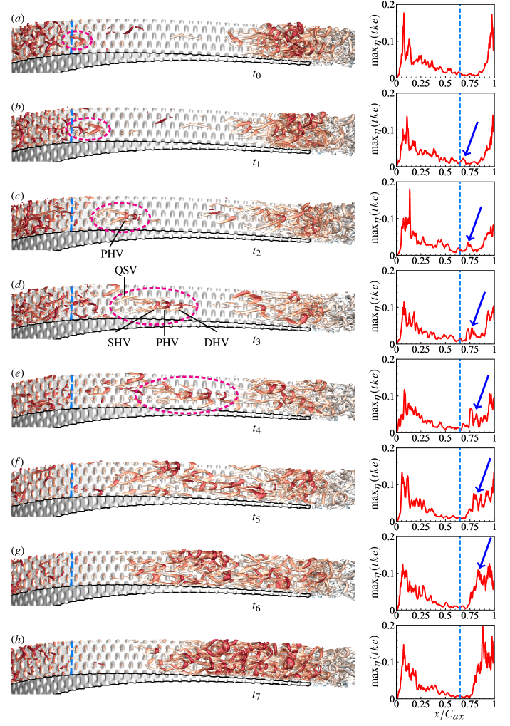
Figure 20: The vortical sturctures on the APG region for $k48\alpha 100$. The blue solid line indicate $x/C_{ax}=0.65$. Meanwhile, the instaneous normal maximum of tke on te suction-side surfacce is averaged in the spanwise direction and plotted against $x/C_{ax}$ for the corresponding snapshorts. PHV, primary hairpin vortex; SHV, secondary hairpin vortex; DHV, downstream hairpin vortex; QSV, quasi-streamwise vortices.

In order to further understand the mechanism of the transition onset for the $k48\alpha 100$ case, we present a zoom-in view of the incipient structures in figure 21. Corresponding to the snapshots in figureS 20(b-d), the contours of $u^{\prime}_{\xi}$ on a tangential-normal plane cut at $z=0.063$ are shown in figureS 21(a-c), and the iso-surfaces of $u^{\prime}_{\xi}$ are presented in figureS 21(d-f), highlighting the formation of the vortical structures represented by the $Q$ iso-surface. It can be seen that the formation of the hairpin structures is accompanied by the evolution of a low-speed region. In particular, impacted by the surface roughness and APG, the streak-like low-speed region lifts up and demonstrates instability, which resembles the varicose mode instability observed during the bypass transition in flat-plate boundary layer (Brandt et al., 2004) and the high-pressure turbine blade (Zhao & Sandberg, 2020).

\begin{overpic}[width=158.70232pt]{fig/u1_fluc_2d_s-n_k39_3491000.png} \put(-5.0,45.0){({a})} \put(-2.0,22.0){{$\eta$}} \put(24.0,39.0){{$u^{\prime}_{\xi}:$}} \end{overpic}

\begin{overpic}[width=158.70232pt]{fig/Q+vel_fluc_3491000_coord_paper_new.png} \put(-2.0,45.0){({d})} \put(95.0,10.0){{$x$}} \put(100.0,52.0){{$z$}} \end{overpic}

\begin{overpic}[width=158.70232pt]{fig/u1_fluc_2d_s-n_k39_3495400.png} \put(-5.0,38.0){({b})} \put(-2.0,22.0){{$\eta$}} \end{overpic}

\begin{overpic}[width=158.70232pt]{fig/Q+vel_fluc_3495400_coord_paper_new.png} \put(-2.0,38.0){({e})} \put(95.0,18.0){{$x$}} \put(100.0,52.0){{$z$}} \end{overpic}

\begin{overpic}[width=158.70232pt]{fig/u1_fluc_2d_s-n_k39_3500000.png} \put(-5.0,38.0){({c})} \put(-2.0,22.0){{$\eta$}} \put(53.0,-3.0){{$\xi$}} \end{overpic}

\begin{overpic}[width=158.70232pt]{fig/Q+vel_fluc_3500000_coord_paper_new.png} \put(-2.0,38.0){({f})} \put(95.0,18.0){{$x$}} \put(100.0,52.0){{$z$}} \end{overpic}

Figure 21: The development of the varicose mode instability indicated by the magenta circle in figure 20. The contours of the tangential velocity fluctuations $u^{\prime}_{\xi}$ on a streamwise-normal plane cut at $z=0.063$ across the hairpin vortex are shown by the instantaneous snapshots at (a) $t=t_{1}$, (b) $t=t_{2}$ and (c) $t=t_{3}$. The iso-surfaces of $u^{\prime}_{\xi}=0.2$ (red), $u^{\prime}_{\xi}=-0.2$ (blue) and $Q=1000$ (green) are also shown at (d) $t=t_{1}$, (e) $t=t_{2}$ and (f) $t=t_{3}$.

In roughness-induced transition, the Kelvin-Helmholtz (K-H) instability within the separated shear layer constitutes a ubiquitous mechanism (Ma & Mahesh, 2023b; Wu et al., 2025). Figure 22 compares time-averaged tangential velocity profiles for cases $k48\alpha 50$ and $k48\alpha 100$ in both FPG and APG regions. A pronounced distinction emerges for the high-wavenumber case, its steeper slope generates stronger reversed flow between the roughness elements. This results in greater momentum deficits and enhanced shear compared to the low-wavenumber case, rendering the shear layer increasingly unstable (Ye et al., 2018). To visually highlight the destabilized shear layer, we present instantaneous contours of vorticity magnitude in figure 23. A detached shear layer lifting away from the roughness elements is observed to show instability in the APG region from around $\xi\approx 0.8$ for case $k48\alpha 100$, consistent with observations by Vadlamani et al. (2018). Conversely, for case $k48\alpha 50$, the flow remains stable without transition, until the significant elevation and breakdown of the shear layer induced by the TE separation bubble as shown in figure 23(a).

\begin{overpic}[width=158.70232pt]{fig/u_x0585_z00750_paper-eps-converted-to.pdf} \put(-4.0,70.0){({a})} \put(-2.0,40.0){{$\eta$}} \put(50.0,-1.0){{$U_{\xi}$}} \end{overpic}

\begin{overpic}[width=158.70232pt]{fig/u_x0800_z00750_paper-eps-converted-to.pdf} \put(-4.0,70.0){({b})} \put(50.0,-1.0){{$U_{\xi}$}} \end{overpic}

Figure 22: Time-averaged velocity profiles in $\xi-\eta$ planes intersecting roughness crests ($z=0.075$) at different streamwise stations: (a) $x/C_{ax}=0.585$, (b) $x/C_{ax}=0.8$.

\begin{overpic}[width=310.4979pt]{fig/omega_contour_k48s50_3500000_paper.png} \put(0.0,18.0){({a})} \put(2.0,11.0){{$\eta$}} \put(97.0,8.0){{$|\omega|$}} \end{overpic}

\begin{overpic}[width=310.4979pt]{fig/omega_contour_k48s100_3500000_paper.png} \put(0.0,18.0){({b})} \put(2.0,11.0){{$\eta$}} \put(50.0,-2.0){{$\xi$}} \put(97.0,8.0){{$|\omega|$}} \end{overpic}

Figure 23: Instantaneous contours of vorticity magnitude on $\xi-\eta$ plane ($z=0.075$). The dashed green lines present $x/C_{ax}=0.1$ and $x/C_{ax}=0.65$. The yellow solid lines denote the zero-isoline of spanwise- and time-averaged tangential velocity. (a) $k48\alpha 50$, (b) $k48\alpha 100$.

One other observation we can draw from figure 23 is that the shear layer in the APG region can be disturbed not only by local roughness elements, but also by disturbances convecting from the LE. Therefore, we recognize that disturbances originating upstream, beyond local instability mechanisms, likely contribute to the contrasting behaviors between cases $k48\alpha 50$ and $k48\alpha 100$. Substantiating this, figures 6 (g,h), 12 (b), 13 (d), and 15 collectively demonstrate significantly stronger disturbances in case $k48\alpha 100$ prior to entering APG region compared to $k48\alpha 50$. To quantify this effect, we acquired time-resolved vorticity signals at two strategic locations: one within the LE region and another in the APG region (see the red and blue probes in figure 23). Sufficiently long signal records were processed with a Hamming window to mitigate Gibbs phenomena prior to Fast Fourier Transform (FFT)-based spectral analysis. The resulting frequency spectra shown in figure 24 reveal near-identical dominant frequencies at both locations, indicating that transition in the APG region is predominantly governed by disturbances convected from the leading-edge flow.

\begin{overpic}[width=310.4979pt]{fig/LE_freq.png} \put(1.0,28.0){({a})} \put(3.0,17.0){{$\phi$}} \put(20.0,24.0){{$f=12.34$}} \end{overpic}

\begin{overpic}[width=310.4979pt]{fig/apg_freq.png} \put(1.0,28.0){({b})} \put(3.0,17.0){{$\phi$}} \put(52.0,1.0){{$f$}} \put(20.0,24.0){{$f=12.02$}} \end{overpic}

Figure 24: Frequency spectra of vorticity signals at different spatial locations for case $k48\alpha 100$. (a) $\xi=0.078$, $\eta=0.013$, (b) $\xi$, $\eta=0.006$

To summarize, for cases with small-amplitude roughness elements, disturbances remain weak throughout the APG region until transition is triggered by flow separation near the trailing edge. In contrast, cases with high-amplitude roughness elements exhibit earlier transition initiation, commencing during or even prior to the APG region. Notably, the streamwise wavenumber exerts negligible influence on transition location in high-roughness configurations. However, for medium-roughness cases $k48$, variations in streamwise wavenumber within a specific range profoundly alter both transition location and mechanism. When the wavenumber increases from $\alpha 50$ to $\alpha 100$, the transition path shifts from separation-induced instability to instability of roughness-induced elevated shear layers, the transition location advances considerably upstream.

5 Conclusion

In the present study, direct numerical simulations of a LPT with roughness elements distributed over the blade surface have been performed, and the roughness height and streamwise wavenumber are varied in a series of fifteen cases to present a systematic study on the complex boundary layer behaviours. For cases with different surface roughness, various paths for transition are observed, including the transition induced by roughness elements in the LE region, transition triggered by TE separation, and also transition induced by shear layer instability in the APG region.

On one hand, the roughness height is indicated to be the dominating factor for suction-side boundary layer transition. Specifically, for cases with large roughness heights, such as the $k64$ and $k80$ cases, the roughness elements in the LE region induce wake structures and the shear layer elevated from the wall quickly breaks down into turbulence. The turbulent fluctuations in these high-amplitude roughness cases sustain through the whole suction-side boundary layer, despite of the stabilizing effect of the FPG region. For cases with relatively small roughness heights (the $k32$ and $k16$ cases), however, the disturbances induced by the LE roughness are suppressed in the FPG region, and the relaminarized boundary layer does not show transition until the TE separation.

The streamwise wavenumber of the distributed roughness, on the other hand, plays an important role in cases with intermediate roughness height, i.e. the $k48$ cases in the present study. The case with smaller wavenumber (the $k48\alpha 50$ case, thus low-level effective slopes) relaminarizes in the FPG region and maintains a laminar mean flow, until boundary layer separation induces prompt breakdown into turbulence. In contrast, the cases with larger wavenumbers (the $k48\alpha 100$ and $k48\alpha 150$ cases) show earlier transition in the APG region, which manages to suppress the mean flow separation near the TE region. Furthermore, the breakdown mechanism for this transition path is suggested to be the instability of the elevated shear layer induced by surface roughness, and the disturbance convected from upstream is implied to play a key role.

We remark that the combined effects of several factors, including the geometric effect at the blade LE and TE, the complex pressure gradient distribution across the turbine vane, and the various roughness heights and wavenumbers, are the key reason for the intriguing boundary layer flow in the present study. Specifically, the roughness elements in the LE region have significant impact on the boundary layer flow, which is presumably due to the small blockage ratio $\delta/k$. Moreover, the roughness elements in the FPG are found to modulate the velocity disturbances in the boundary layer, resulting in the streaks shown by the dispersive velocity. One other interesting observation is the log-linear scaling of the defined roughness function shown in figure 14(d). This indicates the blockage effect of the surface roughness in the FPG region can be well predicted by the geometric parameters of the surface roughness for the present cases, despite that several cases relaminarize in the FPG region while some maintain strong turbulent fluctuations. The result suggests that the present study can support further modelling work on roughness effects on turbine performance.

[Acknowledgements]This work has been supported by the National Natural Science Foundation of China (Grant Nos. 92152202, 12432010 and 12588201).

[Declaration of interests]The authors report no conflict of interest.

Appendix A Computation of the drag coefficient

The total drag consists of the viscous part and the form drag part. The viscous part involves the computation of the wall shear stress, which is typically based on the velocity gradient, i.e. $\tau_{\mathrm{w}}=\mu\nabla\left(\partial U\big/\partial n\right)_{\mathrm{wall}}$. However, it is difficult to determine the velocity gradient at the wall for the cases with the complex roughness topography, which may lead to the inaccurate estimation of the drag coefficient. In the current study, we propose a control volume method to compute the effective wall shear stress as shown in figure A1, which is based on the momentum equation, i.e.

$$\tau_{w}=\left[\int\rho v_{n}\bm{u}dS-\int\bm{n\cdot}\left(-p\mathsfbi{I}+\mathsfbi{\tau}\right)dS-\int\bm{n\cdot}\mathsfbi{R}dS\right]\bm{\cdot\bm{\xi}}/S_{b},$$ (19)

where $\bm{\xi}$ denotes the unit vector in the tangential direction, $\bm{n}$ denotes the unit outer normal vector, $S_{b}$ denotes the surface area of bottom surface of the control volume, $\bm{\tau}$ denotes the viscous stress, and $\bm{R}$ denotes the Reynolds stress.

While this control-volume approach for computing skin friction on rough surfaces has been previously employed (von Deyn et al., 2020), a distinctive feature of our implementation is the explicit retention of the viscous stress term. This formulation enables flexible adjustment of the control-volume height without requiring the upper boundary to extend beyond the boundary layer edge. Furthermore, the streamwise width of the control volume is set equal to the streamwise wavelength $\lambda_{\xi}$, ensuring spatially averaged skin friction results. Equation 19 is applied at each spanwise location, followed by spanwise averaging of the results. Based on the wall shear stress $\tau_{w}$, the drag coefficient is given by

$$C_{d}=\frac{\tau_{w}}{(\rho/2)U_{e}^{*2}}.$$ (20)

\begin{overpic}[width=310.4979pt]{fig/Cf_momentum_sketch.png} \hbox to262.07pt{\vbox to179.25pt{\text{[drawing]}}} \end{overpic}

Figure A1: Schematic visualization of the momentum balance method based control volumes.

References

• Balin & Jansen (2021) Balin, R. & Jansen, K. E. 2021 Direct numerical simulation of a turbulent boundary layer over a bump with strong pressure gradients. J. Fluid Mech. 918, A14.
• Bammert & Milsch (1972) Bammert, K. & Milsch, R. 1972 Boundary layers on rough compressor blades. Turbo Expo: Power for Land, Sea, and Air, vol. ASME 1972 International Gas Turbine and Fluids Engineering Conference and Products Show, p. V001T01A047.
• Bammert & Sandstede (1980) Bammert, K. & Sandstede, H. 1980 Measurements of the boundary layer development along a turbine blade with rough surfaces. J. Eng. Gas Turbines Power 102 (4), 978–983.
• Bogard et al. (1998) Bogard, D. G., Schmidt, D. L. & Tabbita, M. 1998 Characterization and laboratory simulation of turbine airfoil surface roughness and associated heat transfer. ASME J. Turbomach. 120 (2), 337–342.
• Bons (2010) Bons, J. P. 2010 A review of surface roughness effects in gas turbines. ASME J. Turbomach. 132 (2), 021004.
• Boyle & Senyitko (2003) Boyle, R. J. & Senyitko, R. G. 2003 Measurements and predictions of surface roughness effects on the turbine vane aerodynamics. Turbo Expo: Power for Land, Sea, and Air, vol. Volume 6: Turbo Expo 2003, Parts A and B, pp. 291–303.
• Brandt et al. (2004) Brandt, L., Schlatter, P. & Henningson, D. S. 2004 Transition in boundary layers subject to free-stream turbulence. J. Fluid Mech. 517, 167–198.
• Bucci et al. (2021) Bucci, M. A., Cherubini, S., Loiseau, J.-Ch. & Robinet, J.-Ch. 2021 Influence of freestream turbulence on the flow over a wall roughness. Phys. Rev. Fluids 6 (6), 063903.
• Chan et al. (2015) Chan, L., MacDonald, M., Chung, D., Hutchins, N. & Ooi, A. 2015 A systematic investigation of roughness height and wavelength in turbulent pipe flow in the transitionally rough regime. J. Fluid Mech. 771, 743–777.
• Chan et al. (2018) Chan, L., MacDonald, M., Chung, D., Hutchins, N. & Ooi, A. 2018 Secondary motion in turbulent pipe flow with three-dimensional roughness. J. Fluid Mech. 854, 5–33.
• Chung et al. (2021) Chung, D., Hutchins, N., Schultz, M. P. & Flack, K. A. 2021 Predicting the drag of rough surfaces. Ann. Rev. Fluid Mech. 53 (1), 439–471.
• Ciorciari et al. (2014) Ciorciari, R., Kirik, I. & Niehuis, R. 2014 Effects of unsteady wakes on the secondary flows in the linear t106 turbine cascade. ASME J. Turbomach. 136 (9), 091010.
• Citro et al. (2015) Citro, V., Giannetti, F., Luchini, P. & Auteri, F. 2015 Global stability and sensitivity analysis of boundary-layer flows past a hemispherical roughness element 27 (8), 084110.
• Coleman et al. (2018) Coleman, G. N., Rumsey, C. L. & Spalart, P. R. 2018 Numerical study of turbulent separation bubbles with varying pressure gradient and Reynolds number. J. Fluid Mech. 847, 28–70.
• Dassler et al. (2012) Dassler, P., Kožulović, D. & Fiala, A. 2012 An approach for modelling the roughness-induced boundary layer transition using transport equations. In Europ. Congress on Comp. Methods in Appl. Sciences and Engineering, ECCOMAS 2012. Vienna, Austria.
• De Marchis et al. (2015) De Marchis, M., Milici, B. & Napoli, E. 2015 Numerical observations of turbulence structure modification in channel flow over 2D and 3D rough walls. Int. J. Heat Fluid Flow 56, 108–123.
• Deuse & Sandberg (2020) Deuse, M. & Sandberg, R. D. 2020 Implementation of a stable high-order overset grid method for high-fidelity simulations. Comp. Fluids 211, 104449.
• von Deyn et al. (2020) von Deyn, L. H., Forooghi, P., Frohnapfel, B., Schlatter, P., Hanifi, A. & Henningson, D. S. 2020 Direct numerical simulations of bypass transition over distributed roughness. AIAA J. 58 (2), 702–711.
• Ge & Durbin (2015) Ge, X. & Durbin, P. A. 2015 An intermittency model for predicting roughness induced transition. Int. J. Heat Fluid Flow 54, 55–64.
• Hama (1954) Hama, F. R. 1954 Boundary layer characteristics for smooth and rough surfaces. Trans. Soc. Nav. Archit. Mar. Engrs 62, 333–358.
• Hammer et al. (2018) Hammer, F., Sandham, N. D. & Sandberg, R. D. 2018 Large eddy simulations of a low-pressure turbine: Roughness modeling and the effects on boundary layer transition and losses. Turbo Expo: Power for Land, Sea, and Air, vol. Volume 2B: Turbomachinery, p. V02BT41A014.
• Hunt et al. (1988) Hunt, J. C. R., Wray, A. A. & Moin, P. 1988 Eddies, streams, and convergence zones in turbulent flows. In Studying Turbulence Using Numerical Simulation Databases, 2, vol. 1, pp. 193–208.
• Jelly et al. (2022) Jelly, T.O., Ramani, A., Nugroho, B., Hutchins, N. & Busse, A. 2022 Impact of spanwise effective slope upon rough-wall turbulent channel flow. J. Fluid Mech. 951, A1.
• Jelly et al. (2023) Jelly, T. O., Nardini, M., Rosenzweig, M., Leggett, J., Marusic, I. & Sandberg, R. D. 2023 High-fidelity computational study of roughness effects on high pressure turbine performance and heat transfer. Int. J. Heat Fluid Flow 101, 109134.
• Jelly et al. (2025) Jelly, T. O., Nardini, M., Sandberg, R. D., Vitt, P. & Sluyter, G. 2025 Effects of localized non-Gaussian roughness on high-pressure turbine aerothermal performance: Convective heat transfer, skin friction, and the Reynolds’ analogy. ASME J. Turbomach. 147 (5), 051017.
• Jiménez (2004) Jiménez, J. 2004 Turbulent flows over rough walls. Ann. Rev. Fluid Mech. 36 (1), 173–196.
• Joo et al. (2016) Joo, J., Medic, G. & Sharma, O. 2016 Large-eddy simulation investigation of impact of roughness on flow in a low-pressure turbine. Turbo Expo: Power for Land, Sea, and Air, vol. Volume 2C: Turbomachinery, p. V02CT39A053.
• Kennedy et al. (2000) Kennedy, C. A., Carpenter, M. H. & Lewis, R. M. 2000 Low-storage, explicit Runge–Kutta schemes for the compressible Navier–Stokes equations. Appl. Numer. Maths. 35 (3), 177–219.
• Kim & Sandberg (2012) Kim, J. W. & Sandberg, R. D. 2012 Efficient parallel computing with a compact finite difference scheme. Comp. Fluids 58, 70–87.
• Kind et al. (1998) Kind, R. J., Serjak, P. J. & Abbott, M. W. P. 1998 Measurements and prediction of the effects of surface roughness on profile losses and deviation in a turbine cascade. ASME J. Turbomach. 120 (1), 20–27.
• Klein et al. (2003) Klein, M., Sadiki, A. & Janicka, J. 2003 A digital filter based generation of inflow data for spatially developing direct numerical or large eddy simulations. J. Comp. Phys. 186 (2), 652–665.
• Lee et al. (2011) Lee, J. H., Sung, H. J. & Krogstad, P.$\rm~\mathring{A}$. 2011 Direct numerical simulation of the turbulent boundary layer over a cube-roughened wall. J. Fluid Mech. 669, 397–431.
• Liu et al. (2020) Liu, Z., Zhao, Y., Chen, S., Yan, C. & Cai, F. 2020 Predicting distributed roughness induced transition with a four-equation laminar kinetic energy transition model. Aerosp. Sci. Technol. 99, 105736.
• Loiseau et al. (2014) Loiseau, J., Robinet, J., Cherubini, S. & Leriche, E. 2014 Investigation of the roughness-induced transition: global stability analyses and direct numerical simulations. J. Fluid Mech. 760, 175–211.
• Ma et al. (2020) Ma, G. Z., Xu, C. X., Sung, H. J. & Huang, W. X. 2020 Scaling of rough-wall turbulence by the roughness height and steepness. J. Fluid Mech. 900, R7.
• Ma et al. (2022) Ma, G. Z., Xu, C. X., Sung, H. J. & Huang, W. X. 2022 Scaling of rough-wall turbulence in a transitionally rough regime. Phys. Fluids 34 (3), 031701.
• Ma et al. (2023) Ma, G. Z., Xu, C. X., Sung, H. J. & Huang, W. X. 2023 Outer-layer similarity and energy transfer in a rough-wall turbulent channel flow. J. Fluid Mech. 968, A18.
• Ma & Mahesh (2022) Ma, R. & Mahesh, K. 2022 Global stability analysis and direct numerical simulation of boundary layers with an isolated roughness element. J. Fluid Mech. 949, A12.
• Ma & Mahesh (2023a) Ma, R. & Mahesh, K. 2023a Boundary layer transition due to distributed roughness: effect of roughness spacing. J. Fluid Mech. 977, A27.
• Ma & Mahesh (2023b) Ma, R. & Mahesh, K. 2023b Boundary layer transition due to distributed roughness: effect of roughness spacing. J. Fluid Mech. 977, A27.
• Marxen & Zaki (2019) Marxen, O. & Zaki, T. A. 2019 Turbulence in intermittent transitional boundary layers and in turbulence spots. J. Fluid Mech. 860, 350–383.
• Michelassi et al. (2015) Michelassi, V., Chen, L.-W., Pichler, R. & Sandberg, R. D. 2015 Compressible direct numerical simulation of low-pressure turbines—Part II: Effect of inflow disturbances. ASME J. Turbomach. 137 (7), 071005.
• Muppidi & Mahesh (2012) Muppidi, S. & Mahesh, K. 2012 Direct numerical simulations of roughness-induced transition in supersonic boundary layers. J. Fluid Mech. 693, 28–56.
• Napoli et al. (2008) Napoli, E., Armenio, V. & De Marchis, M. 2008 The effect of the slope of irregularly distributed roughness elements on turbulent wall-bounded flows. J. Fluid Mech. 613, 385–394.
• Nardini et al. (2023a) Nardini, M., Jelly, T. O., Kozul, M., Sandberg, R. D., Vitt, P. & Sluyter, G. 2023a Direct numerical simulation of transitional and turbulent flows over multi-scale surface roughness—Part II: The Effect of roughness on the performance of a high-pressure turbine blade. ASME J. Turbomach. 146 (3), 031009.
• Nardini et al. (2023b) Nardini, M., Kozul, M., Jelly, T. O. & Sandberg, R. D. 2023b Direct numerical simulation of transitional and turbulent flows over multi-scale surface roughness—Part I: Methodology and challenges. ASME J. Turbomach. 146 (3), 031008.
• Nikuradse (1933) Nikuradse, J. 1933 Strömungsgesetze in rauhen Rohren. VDI-Forschungsheft 361, 1.
• Nolan & Zaki (2013) Nolan, K. P. & Zaki, T. A. 2013 Conditional sampling of transitional boundary layers in pressure gradients. J. Fluid Mech. 728, 306–339.
• Otsu (1979) Otsu, N. 1979 A threshold selection method from gray-level histograms. IEEE Trans. Syst. Man Cybern. 9 (1), 62–66.
• Raupach et al. (1991) Raupach, M. R., Antonia, R. A. & Rajagopalan, S. 1991 Rough-wall turbulent boundary layers. Appl. Mech. Rev. 44 (1), 1–25.
• Raupach & Thom (1981) Raupach, M. R. & Thom, A. S. 1981 Turbulence in and above plant canopies. Ann. Rev. Fluid Mech. 13 (1), 97–129.
• Reynolds & Hussain (1972) Reynolds, W. C. & Hussain, A. K. M. F. 1972 The mechanics of an organized wave in turbulent shear flow. Part 3. Theoretical models and comparisons with experiments. J. Fluid Mech. 54 (2), 263–288.
• Roberts & Yaras (2005) Roberts, S. K. & Yaras, M. I. 2005 Effects of surface-roughness geometry on separation-bubble transition. ASME J. Turbomach. 128 (2), 349–356.
• Sandberg et al. (2015) Sandberg, R. D., Michelassi, V., Pichler, R., Chen, L. & Johnstone, R. 2015 Compressible direct numerical simulation of low-pressure turbines—Part I: Methodology. ASME J. Turbomach. 137 (5), 051011.
• Sandberg & Sandham (2006) Sandberg, R. D. & Sandham, N. D. 2006 Nonreflecting zonal characteristic boundary condition for direct numerical simulation of aerodynamic sound. AIAA J. 44 (2), 402–405.
• Sayadi et al. (2013) Sayadi, T., Hamman, C. W. & Moin, P. 2013 Direct numerical simulation of complete H-type and K-type transitions with implications for the dynamics of turbulent boundary layers. J. Fluid Mech. 724, 480–509.
• Schlanderer et al. (2017) Schlanderer, S. C., Weymouth, G. D. & Sandberg, R. D. 2017 The boundary data immersion method for compressible flows with application to aeroacoustics. J. Comp. Phys. 333, 440–461.
• Schlichting (1968) Schlichting, H. 1968 Boundary Layer Theory. New York: McGraw-Hill.
• Schultz (2007) Schultz, M. P. 2007 Effects of coating roughness and biofouling on ship resistance and powering. Biofouling 23 (5), 331–341.
• Schultz & Flack (2009) Schultz, M. P. & Flack, K. A. 2009 Turbulent boundary layers on a systematically varied rough wall. Phys. Fluids 21 (1), 015104.
• Spalart & Watmuff (1993) Spalart, P. R. & Watmuff, J. H. 1993 Experimental and numerical study of a turbulent boundary layer with pressure gradients. J. Fluid Mech. 249, 337–371.
• Stadtmüller (2001) Stadtmüller, P 2001 Investigation of wake-induced transition on the LP turbine cascade T106A-EIZ. DFG-Verbundprojekt Fo 136 (11).
• Tao (2009) Tao, J. J. 2009 Critical instability and friction scaling of fluid flows through pipes with rough inner surfaces. Phys. Rev. Lett. 103, 264502.
• Tarada & Suzuki (1993) Tarada, F. & Suzuki, M. 1993 External heat transfer enhancement to turbine blading due to surface roughness. Turbo Expo, vol. Volume 2, p. V002T08A006.
• Thakkar et al. (2017) Thakkar, M., Busse, A. & Sandham, N. 2017 Surface correlations of hydrodynamic drag for transitionally rough engineering surfaces. J. Turbul. 18 (2), 138–169.
• Townsend (1976) Townsend, A.A. 1976 The Structure of Turbulent Shear Flow. Cambridge University Press.
• Vadlamani et al. (2018) Vadlamani, N. R., Tucker, P. G. & Durbin, P. 2018 Distributed roughness effects on transitional and turbulent boundary layers. Flow Turbul. Combust. 100 (3), 627–649.
• Wang et al. (2021) Wang, M., Lu, X., Yang, C., Zhao, S. & Zhang, Y. 2021 Numerical investigation of distributed roughness effects on separated flow transition over a highly loaded compressor blade. Phys. Fluids 33 (11), 114104.
• Wei et al. (2017) Wei, L., Ge, X., George, J. & Durbin, P. 2017 Modeling of laminar-turbulent transition in boundary layers and rough turbine blades. ASME J. Turbomach. 139 (11), 111009.
• White (1991) White, F. M. 1991 Viscous Fluid Flow. McGraw-Hill, New York.
• Wu et al. (2025) Wu, H., Yang, x., Li, G. & Yin, Z. 2025 Interaction of freestream turbulence and surface roughness in separation-induced transition. Phys. Rev. Fluids 10 (1), 013903.
• Ye et al. (2018) Ye, Q., Schrijer, F. F. J. & Scarano, F. 2018 On Reynolds number dependence of micro-ramp-induced transition. J. Fluid Mech. 837, 597–626.
• Zhao & Sandberg (2020) Zhao, Y. & Sandberg, R. D. 2020 Bypass transition in boundary layers subject to strong pressure gradient and curvature effects. J. Fluid Mech. 888, A4.
• Zhao & Sandberg (2021) Zhao, Y. & Sandberg, R. D. 2021 High-fidelity simulations of a high-pressure turbine vane subject to large disturbances: Effect of exit Mach number on losses. ASME J. Turbomach. 143 (9), 091002.
• Zhao et al. (2016) Zhao, Y., Yang, Y. & Chen, S. 2016 Evolution of material surfaces in the temporal transition in channel flow. J. Fluid Mech. 793, 840–876.
• Zhou et al. (1999) Zhou, J., Adrian, R. J., Balachandar, S. & Kendall, T. M. 1999 Mechanisms for generating coherent packets of hairpin vortices in channel flow. J. Fluid Mech. 387, 353–396.