WimPyC: an extension module of WimPyDD for the calculation of WIMP capture in celestial bodies

Abstract

We introduce WimPyC, a Python code for the calculation of the capture rate of Weakly Interacting Massive Particles (WIMPs) by celestial bodies through nuclear scattering in the optically thin regime. WimPyC is an extension of the WimPyDD code, that calculates WIMP–nucleus scattering signals in direct detection (DD) experiments, and allows to combine DD and capture in celestial bodies in virtually any scenario within the framework of Galilean–invariant non–relativistic effective theory (NREFT), including inelastic scattering, an arbitrary WIMP spin and a generic WIMP velocity distribution in the Galactic halo. WimPyDD and WimPyC are suitable for both top–down approaches, where the interaction operators of a high–energy physics model are matched to those of the NREFT, and to bottom–up studies, where the Wilson coefficients of the NREFT are explored in a model–independent way and/or where the velocity distribution is written in terms of a superposition of streams taken as free parameters. As in the case of WimPyDD WimPyC exploits the factorization of the three main components that enter in the calculation of the capture rate: i) the Wilson coefficients that encode the dependence of the signals on the ultraviolet completion of the effective theory; ii) a response function that depends on the nuclear physics; iii) the halo function that depends on the WIMP velocity distribution. In WimPyC these three components are calculated and stored separately for later interpolation and combined together only as the last step of the signal evaluation procedure. This makes the phenomenological study of the capture rate with WimPyC transparent and improves computational speed.

CQUeST-2025-0764

PROGRAM SUMMARY

Module Title: WimPyC
Licensing provisions: MIT
Programming language: Python3
First release: v2.0.0
Official repository: HEPForge
Home page: wimpydd.hepforge.org

Nature of problem
Stars and planets in our galaxies are expected to be embedded in an extended dark matter halo made of WIMPs. When they cross a celestial body DM particles can lose energy and become gravitationally captured by the same WIMP–nucleus scattering process driving direct detection in terrestrial detectors. The rate at which this process occurs is called the capture rate, and, under proper conditions, can lead to a dense population of DM particles inside the celestial body with a consequent enhancement of their annihilation rate. This can produce indirect observational signatures such as a flux of high–energy neutrinos from the celestial body, or an increase in its temperature/luminosity. Combining direct and indirect signals can potentially improve our chance to detect WIMPs, but can be cumbersome especially in generalized scenarios.

Solution method:
The WimPyC module seamlessly integrates with the WimPyDD code, that calculates WIMP–nucleus scattering signals in direct detection experiments. It allows to calculate the WIMP capture rate in virtually any scenario, including an arbitrary spin, inelastic scattering, and a non-standard halo function. Each ingredient, including the celestial body, can be set up independently in an easy and intuitive way.

1 Introduction

In Ref. [1] we introduced WimPyDD, a customizable, object–oriented Python code for the calculation of expected rates of WIMP–nucleus scattering events in direct detection (DD) experiments in underground solid and liquid state detectors within the frame of the most general Non–Relativistic Effective Field Theory (NREFT) WIMP–nucleon Hamiltonian [2, 3] In the present paper we wish to introduce a new WimPyDD module called WimPyC, in order to extend the code to the calculation of WIMP capture in celestial bodies.

All celestial bodies such as the Sun, the Earth, star, planets and stellar remnants are expected to be embedded in a dark matter halo made of WIMPs. When a WIMP crosses the celestial body it can lose energy and become gravitationally captured. This can eventually lead to a dense population of WIMPs that enhances their annihilation rate, potentially producing indirect observational signatures such as a flux of high–energy neutrinos [4, 5], an increase in the temperature/luminosity of the celestial body [6], or even to alterations in the evolutionary history of stars [7, 8].

Since DD and capture in celestial bodies are driven by the same WIMP–nucleus scattering process, combining the two signals can be useful to extend the sensitivity to the WIMP parameter space. For instance, indicating with $u$ the WIMP speed in the reference frame of the solar system, due to the energy threshold DD experiments are insensitive to low values of $u$, while capture in the Sun is suppressed or impossible at high values of $u$, and only combining the two signals it is possible to obtain halo–independent bounds that, by probing the full range of incoming WIMP speeds, do not depend on the specific choice of the velocity distribution [9, 10, 11, 12]. Moreover, when the WIMP–nucleus interaction is described by NREFT scattering rate is a quadratic form in the parameter space of the couplings that has flat directions corresponding to large cancellations among the Wilson coefficients of the effective Hamiltonian [13]. Since each nuclear target has different flat directions the bounds on the Wilson coefficients can be improved by exploiting the complementarity among the targets used in DD and those that drive WIMP capture in celestial bodies. The WimPyC module handles WIMP-nucleus scattering using the same classes, routines and input data of WimPyDD, allowing to jointly analyze DD and WIMP capture in a seamless way.

Several codes exist in the literature whose tasks partially overlap those performed by WimPyC: Asteria [14], micrOMEGAs [15], DarkSUSY [16], DaMaSCUS [17, 18], DaMaSCUS-EarthCapture [19], and Capt’n General [20]. All codes treat the WIMP–nucleus scattering process as elastic, and most of them handle only Spin-Independent (SI) and Spin-Dependent (SD) interactions in the Earth and the Sun, in the optically thin regime. The treatment of multiple scattering is included in Asteria for the Sun, the Earth and for Jupiter, and in DaMaSCUS only for the Earth. Capt’n General handles NREFT interactions for a spin 1/2 particle (it can also read Solar or stellar model files and be interfaced with the MESA stellar evolution code). DarkSUSY allows to choose among different solar models and includes predefined velocity distributions, whereas micrOMEGAs is flexible in the definition of the halo function. With the exception of the latter and of DarkSUSY all codes assume a Maxwellian WIMP velocity distribution. In comparison with other codes WimPyC only handles the optically thin regime. On the other hand, it allows to implement capture in virtually any celestial body and is completely flexible on the particle physics scenario and on the WIMP velocity distribution. Moreover, being an extension of WimPyDD, it is particularly suitable to study the correlation and complementarity with direct detection also with halo–independent [10, 11, 12] and matricial [21, 13] techniques.

The paper is organized as follows. In Section 2 we summarize the expressions used by WimPyC to calculate the capture rate in the optically thin regime and optimized for numerical evaluation; in Section 3 the components of the WimPyC module are introduced: the isotope class in 3.3.2, the load_response_functions_capture routine in 3.4; the celestial_body class in 3.3.1; in Section 3.2 the wimp_capture, wimp_capture_matrix and wimp_capture_accurate signal routines are introduced, as well as wimp_capture_geom for the geometrical capture rate. Several explicit examples of how to use the WimPyC module, as well as the comparison of the corresponding WimPyC output to published results are provided in Section 4. Appendix A describes in detail how to initialize a new celestial body; a description of the pre–defined celestial_body objects included in the WimPyC distribution is provided in Appendix B; the wimp_annihilation routine that handle equilibrium between capture and annihilation is described in Appendix C. Finally, the accuracy of the interpolation method used to improve the computational speed in the calculation of the capture rate is discussed in Appendix D.

2 WIMP capture in a celestial body

In the optically–thin limit the capture rate of WIMPs of mass $m_{\chi}$ in a celestial body of radius $R_{\odot}$ is given by [5]:

$$C_{opt}\ = \left(\frac{\rho_{\chi}}{m_{\chi}}\right)\hskip 1.42262pt\int^{R_{\odot}}_{0}dr\hskip 1.42262pt4\pi r^{2}\sum_{T}\frac{dC_{opt,T}(r)}{dV}$$ (2.1)

$$\frac{dC_{opt,T}(r)}{dV}\ = \int du\hskip 1.42262ptf(u)\hskip 1.42262pt\frac{1}{u}\hskip 1.42262ptw(u,r)^{2}$$ (2.2)

$$\times~\eta_{T}(r)\hskip 1.42262pt\hskip 1.42262pt\Theta(E^{\chi}_{\rm max}-E^{\chi}_{\rm cap})\int_{E_{1}(u,r)}^{E_{2}(u,r)}\frac{d\sigma_{T}}{dE_{R}}(w)dE_{R}$$

with $\rho_{\chi}$ the density of DM at the position of the celestial body, $\eta_{T}(r)$ the number density profile for target nucleus $T$, $u$ the asymptotic speed of the incoming WIMP at large distance from the center of the celestial body, $w(u,r)^{2}=u^{2}+v_{\rm esc}(r)^{2}$ the WIMP speed at the target position, $v_{\rm esc}(r)$ the escape speed at distance $r$ from its center, and:

$$E_{1}(u,r) = {\rm max}[E^{\chi}_{\rm min}(u,r),E^{\chi}_{\rm cap}(u)]$$

$$E_{2}(u,r) = E^{\chi}_{\rm max}(u,r)$$ (2.3)

$$E^{\chi}_{\rm min,\rm max}(u,r) = \frac{1}{2}m_{\chi}w^{2}\left[1-\frac{\mu^{2}_{\chi T}}{m^{2}_{T}}\left(1\pm\frac{m_{T}}{m_{\chi}}\sqrt{1-\frac{v^{2}_{T*}}{w^{2}}}\right)^{2}\right]-\delta,$$ (2.4)

$$E^{\chi}_{\rm cap}(u) = \frac{1}{2}m_{\chi}u^{2}-\delta.$$ (2.5)

In the equations above $m_{T}$ is the mass of the nuclear target, $\mu_{\chi T}$ is the WIMP–nucleus reduced mass and $\delta$ the mass splitting in case of the Inelastic Dark Matter (IDM) scenario when the DM particle $\chi$ interacts with atomic nuclei exclusively by making a transition to a second state $\chi^{\prime}$ with mass $m_{\chi^{\prime}}$ = $m_{\chi}$ + $\delta$ endothermally ($\delta>0$) [22] or exothermally ($\delta<0$) [23] (the elastic case is recovered when $\delta$ =0). In particular, $E^{\chi}_{\rm min,\rm max}(u,r)$ represent the minimal and maximal recoil energies of a WIMP with incoming speed $w$ while $E^{\chi}_{\rm cap}(u)$ is the minimal recoil energy for capture, i.e. for the outgoing WIMP speed to be below the escape velocity after the scattering process. A peculiar feature of IDM is that WIMP–nucleus scattering has a velocity threshold given by:

$$v_{T^{*}}\equiv\left\{\begin{aligned} \sqrt{\frac{2\delta}{\mu_{\chi T}}},\quad\text{if}\;\delta>0\\ 0,\quad\text{if}\;\delta\leq 0\,.\end{aligned}\right.$$ (2.6)

Specifically, the condition $E^{\chi}_{\rm max}>E^{\chi}_{\rm cap}$ in the integrals of Eq. (2.2) ensures that $w>v_{T^{*}}$ and that the scattering process is kinematically possible.

Moreover:

$$\frac{d\sigma_{T}}{dE_{R}}(w)=\frac{2m_{T}}{4\pi}\frac{c^{2}}{w^{2}}\left[\frac{1}{2j_{\chi}+1}\frac{1}{2j_{T}+1}\sum_{spin}|{\cal M}(q)|^{2}_{T}\right],$$ (2.7)

is the WIMP–nucleus differential scattering cross section in terms of the scattering amplitude averaged over the initial WIMP and target spins. In the non–relativistic effective theory described by the Hamiltonian [2, 3, 24, 25, 26]:

$${\bf\mathcal{H}}(x_{i},q) = \sum_{\tau=0,1}\sum_{j}c_{j}^{\tau}(x_{i},q)\mathcal{O}_{j}({\bf{q}})\,t^{\tau},$$ (2.8)

the scattering amplitude is given by:

$$\frac{1}{2j_{\chi}+1}\frac{1}{2j_{T}+1}\sum_{spin}|{\cal M}(q)|^{2}_{T}=\frac{4\pi}{2j_{T}+1}\sum_{\tau\tau^{\prime}}\sum_{l}R_{l}^{\tau\tau^{\prime}}(q,v)W_{l,T}^{\tau\tau^{\prime}}(q).$$ (2.9)

In Eq. (2.8) we have explicitly written the dependence of the Wilson coefficients on some parameters $x_{i}$ (which can include the WIMP mass $m_{\chi}$ and the mass splitting $\delta$) arising from the matching of the Wilson coefficients of the low–energy effective theory to its ultraviolet completion, and on the transferred momentum $q=\sqrt{2m_{T}E_{R}}$ (for instance through a propagator). All $\mathcal{O}_{j}$ operators for $j_{\chi}\leq$ 1/2, and some for $j_{\chi}$ = 1 are listed, for instance, in Table B.1 of [1]. Moreover, in Eq. (2.8), $t^{0}=1$, $t^{1}=\tau_{3}$ denote the $2\times 2$ identity and third Pauli matrix in the nucleon isospin space, respectively, and the isoscalar and isovector Wilson coefficients coupling $c^{0}_{j}$ and $c^{1}_{j}$ are related to those to protons and neutrons $c^{p}_{j}$ and $c^{n}_{j}$ by $c^{p}_{j}=(c^{0}_{j}+c^{1}_{j})/2$ and $c^{n}_{j}=(c^{0}_{j}-c^{1}_{j})/2$.

In Eq. (2.9) the WIMP and nuclear physics are factorized in the two $R_{l}^{\tau\tau^{\prime}}$ and $W_{l,T}^{\tau\tau^{\prime}}$ functions, respectively, with $\tau,\tau^{\prime}=0,1$ the nuclear isospin while $l$=$M$,$\Sigma^{\prime\prime}$ ,$\Sigma^{\prime}$,$\Phi^{\prime\prime}$, $\Phi^{\prime\prime}M$, $\tilde{\Phi}^{\prime}$,$\Delta$, $\Delta\Sigma^{\prime}$ represent one of the possible nuclear interaction types, in the single–particle interaction limit [2, 3]. Explicit expressions of the WIMP response functions $R_{l}^{\tau\tau^{\prime}}$ are provided in [3] for the set of operators ${\cal O}_{j}$ ($j=1,3,...,15$) valid for $j_{\chi}=0,1/2$ and in [26] for the set of operators ${\cal O}_{X,l,s}$ for an arbitrary $j_{\chi}$ (for details on how WimPyDD handles the two set of interaction operators see Appendix B of [1]). In particular, the WIMP response functions can be decomposed as:

$$R_{l}^{\tau\tau^{\prime}}(q,w)=R_{0,l}^{\tau\tau^{\prime}}(q)+R_{1,l}^{\tau\tau^{\prime}}(q)(w^{2}-v_{T,min}^{2}),$$ (2.10)

where:

$$v_{T,min}(E_{R})=\frac{1}{\sqrt{2m_{T}E_{R}}}\left|\frac{m_{T}E_{R}}{\mu_{\chi T}}+\delta\right|,$$ (2.11)

is the minimal speed an incoming WIMP needs to have in the target reference frame to deposit energy $E_{R}$, with $v_{T,min}\geq v_{T*}$ ($v_{T,min}=v_{T*}$ when $E_{R}=E_{R*}=\mu_{\chi T}\delta/m_{T}$).

As a consequence, also the cross section in Eq. (2.7) can be written as:

$$\frac{d\sigma_{T}}{dE_{R}}(w)=\frac{1}{w^{2}}\left\{\left(\frac{d\tilde{\sigma}_{T}}{dE_{R}}\right)_{0}+\left(\frac{d\tilde{\sigma}_{T}}{dE_{R}}\right)_{1}\frac{w^{2}-v_{T,min}^{2}}{c^{2}}\right\}.$$ (2.12)

As far as the nuclear response functions $W_{l,T}^{\tau\tau^{\prime}}$ are concerned, their power/exponential expansions have been provided in [3] for most targets $T$ used in DD experiments and in [27] for those present in typical celestial bodies such as stars, planets and white dwarfs.

If the scattering process is driven by the Hamiltonian of Eq. (2.8) the functions $(d\tilde{\sigma}_{T}/dE_{R})_{i}$ appearing in Eq. (2.12) are quadratic in the Wilson coefficients of the effective theory, that can be factored out:

$$\left(\frac{d\tilde{\sigma}_{T}}{dE_{R}}\right)_{i}(E_{R})=\sum_{j,k}c_{j}^{\tau}(x_{i},q_{0})c_{k}^{\tau^{\prime}}(x_{i},q_{0}^{\prime})\left[\frac{d\tilde{\sigma}_{T}^{i}}{dE_{R}}\right]_{jk}^{\tau\tau^{\prime}}(E_{R}),\,\,i=0,1.$$ (2.13)

In the expression above $q_{0}$, $q_{0}^{\prime}$ are arbitrary momentum scales in the case when the Wilson coefficients $c_{j}^{\tau}$, $c_{k}^{\tau^{\prime}}$ have an explicit dependence on $q$. Using in Eq. (2.12) the explicit expression of the square of $v_{T,min}(E_{R})$:

$$v_{T,min}(E_{R})^{2}=\frac{m_{T}}{2\mu_{\chi T}^{2}}E_{R}+\frac{\delta^{2}}{2m_{T}}\frac{1}{E_{R}}+\frac{\delta}{\mu_{\chi T}}$$ (2.14)

one can define:

$$\left[\frac{d\tilde{\sigma}_{T}^{1E}}{dE_{R}}\right]_{jk}^{\tau\tau^{\prime}}(E_{R})\equiv E_{R}\left[\frac{d\tilde{\sigma}_{T}^{1}}{dE_{R}}\right]_{jk}^{\tau\tau^{\prime}}(E_{R})$$

$$\left[\frac{d\tilde{\sigma}_{T}^{1E^{-1}}}{dE_{R}}\right]_{jk}^{\tau\tau^{\prime}}(E_{R})\equiv\frac{1}{E_{R}}\left[\frac{d\tilde{\sigma}_{T}^{1}}{dE_{R}}\right]_{jk}^{\tau\tau^{\prime}}(E_{R}),$$ (2.15)

leading to the following set of four differential response functions:

$$\left[\frac{d\tilde{\sigma}_{T}^{a}}{dE_{R}}\right]_{jk}^{\tau\tau^{\prime}}=\left\{\left[\frac{d\tilde{\sigma}_{T}^{0}}{dE_{R}}\right]_{jk}^{\tau\tau^{\prime}},\left[\frac{d\tilde{\sigma}_{T}^{1}}{dE_{R}}\right]_{jk}^{\tau\tau^{\prime}},\left[\frac{d\tilde{\sigma}_{T}^{1E}}{dE_{R}}\right]_{jk}^{\tau\tau^{\prime}},\left[\frac{d\tilde{\sigma}_{T}^{1E^{-1}}}{dE_{R}}\right]_{jk}^{\tau\tau^{\prime}}\right\}$$ (2.16)

and the corresponding integrated response functions:

$$\left[\bar{\sigma}^{a}_{T}\right]_{jk}^{\tau\tau^{\prime}}(E_{R})\equiv\int_{0}^{E_{R}}dE^{\prime}_{R}\left[\frac{d\tilde{\sigma}_{T}^{a}}{dE_{R}}\right]_{jk}^{\tau\tau^{\prime}}(E_{R}^{\prime}),\,\,\,a=0,1,1E,1E^{-1}.$$

(2.17)

Using Eqs. (2.12) and (2.13) in (2.2) the capture rate can then be written as:

$$\frac{dC_{opt,T}(r)}{dV}=\sum_{k=1}^{N_{s}}\delta\eta_{k}\times\frac{dC_{opt,T}}{dV}(r,u_{k})$$

$$\frac{dC_{opt,T}}{dV}(r,u_{k})\equiv\sum_{ij}\sum_{\tau\tau^{\prime}}c_{j}^{\tau}(x_{i},q_{0})c_{k}^{\tau^{\prime}}(x_{i},q_{0}^{\prime})$$

$$\left\{\frac{1}{u_{k}}\left[\bar{{\sigma}}^{0}_{T}\right]_{jk}^{\tau\tau^{\prime}}(E_{R})+(\frac{u_{k}}{c^{2}}-\frac{\delta}{\mu_{\chi T}u_{k}})\left[\bar{{\sigma}}^{1}_{T}\right]_{jk}^{\tau\tau^{\prime}}(E_{R})\right.$$

$$\left.-\frac{m_{T}}{2\mu_{\chi T}^{2}u_{k}}\left[\bar{{\sigma}}^{1E}_{T}\right]_{jk}^{\tau\tau^{\prime}}(E_{R})-\frac{\delta^{2}}{2m_{T}u_{k}}\left[\bar{{\sigma}}^{1E^{-1}}_{T}\right]_{jk}^{\tau\tau^{\prime}}(E_{R})\right\}^{E_{2}(u_{k},r)}_{E_{1}(u_{k},r)},$$

with $\{f(E_{R})\}_{E_{1}}^{E_{2}}\equiv f(E_{2})-f(E_{1})$. Moreover, in Eq. (LABEL:eq:capture_master) the WIMP speed distribution $f(v)\equiv 1/(4\pi)\int d\Omega v^{2}f(\vec{v})$ is written as a superposition of streams:

$$f(u)=\sum_{k}^{N_{s}}\lambda_{k}\delta(u-u_{k}),$$ (2.19)

so that the halo-function is written as:

$$\eta(u) = \int_{u}^{\infty}\frac{f(u^{\prime})}{u^{\prime}}\,du^{\prime}=\sum_{k=1}^{N_{s}}\delta\eta_{k}\theta(u_{k}-u),$$

$$\delta\eta_{k} = \lambda_{k}/u_{k}.$$ (2.20)

Combined with the radial integration of Eq. (2.1), Eq. (LABEL:eq:capture_master) serves as the master formula used by WimPyC to calculate the capture rate through Eq. (2.2). It has the same structure of Eq. (20) of Ref. [1] used by WimPyDD to calculate expected rates for DD, and it exploits explicitly the factorization of the Wilson coefficients $c_{j}^{\tau}$, the response functions $\left[\bar{\sigma}^{a}_{T}\right]_{jk}^{\tau\tau^{\prime}}(E_{R})$ ($a$=0, 1, 1$E$, 1$E^{-1}$) and of the halo functions $\delta\eta_{k}^{(0,1)}$ (see Appendix E of [1] for how to implement the latter in WimPyDD). Since the response functions $\left[\bar{\sigma}^{a}_{T}\right]_{jk}^{\tau\tau^{\prime}}(E_{R})$ depend only on the single external argument $E_{R}$ WimPyC speeds up the calculation by tabulating each $\left[\bar{\sigma}^{a}_{T}\right]_{jk}^{\tau\tau^{\prime}}(E_{R})$ for later interpolation. In particular such tables do not depend on the WIMP mass $m_{\chi}$ and on the mass splitting $\delta$, that only enter in the mapping between the $u_{k}$ values and the energies $E_{1}(u_{k})$ and $E_{2}(u_{k})$ at which the response functions in the tables are interpolated. We have extensively verified that such interpolation method leads to accurate results, although, for completeness and validation purposes WimPyC also provides an alternative (and slower) routine that performs the full integrations of Eq. (2.2).

In analogy to DD rates, thanks to the factorization in Eq. (2.13) the capture rate can be seen as a quadratic form in the couplings:

$$C_{opt}=c^{T}\cdot{\cal M}\cdot c,$$

$$c=\{c_{j}^{\tau}\}.$$ (2.21)

This allows to apply matricial techniques when analyzing the multi–dimensional parameter space of the WIMP effective Hamiltonian [28, 21, 13]. WimPyC includes a dedicated routine for the calculation of the matrix ${\cal M}$ (see example in Section 4.8).

Moreover, again in the same way of DD, using $\delta\eta_{k}^{(0,1)}=\lambda_{k}^{(0,1)}/v_{k}$ Eqs. (2.2,LABEL:eq:capture_master) can be recast in the form:

$$C_{opt}=\sum_{k=1}^{N_{s}}\lambda_{k}{\cal H}_{C}(u_{k}),$$ (2.22)

$${\cal H}_{C}(u_{k})=\left(\frac{\rho_{\chi}}{m_{\chi}}\right)\hskip 1.42262pt\int^{R_{\odot}}_{0}dr\hskip 1.42262pt4\pi r^{2}\sum_{T}\frac{1}{u_{k}}\frac{dC_{opt,T}(r,u_{k})}{dV},$$ (2.23)

which corresponds to the expression:

$$C_{opt}=\int_{0}^{\infty}du{\cal H}_{C}(u)f(u),$$ (2.24)

when the velocity distribution $f(u)$ is parameterized in terms of a sum of streams using Eq. (2.19). Eq. (2.24) shows that, by making use of the master formula of Eq. (LABEL:eq:capture_master), WimPyC is very suitable to apply the halo-independent method discussed in [29, 30, 31], where the velocity distribution or the halo function is written in terms of a set of free parameters (namely, the velocities $v_{k}$ and either the $\lambda_{k}$’s or the $\eta_{k}$’s, see the discussion in Section 2.1 of [1]). This will be illustrated in the example of Section 4.9.

Eqs. (2.2, LABEL:eq:capture_master) assume that a WIMP is captured for good after a single scattering event off a nuclear target at distance $r$ from the center of the celestial body, which brings the WIMP below the escape velocity $v_{esc}(r)$. Specifically, after the first scattering the WIMP is assumed to be locked into a bound orbit so that over the age of the system it keeps crossing the celestial body scattering time and again, eventually thermalizing with the nuclei in its environment and settling into a distribution peaked at its center.

Thanks to gravitational acceleration capture allows to probe the WIMP–nucleus scattering process at WIMP speeds not within the reach of terrestrial detectors, potentially improving the sensitivity to the WIMP parameter space. This is especially true in specific scenarios, such as inelastic scattering [34]. However, Eq. (LABEL:eq:capture_master) is based on the NREFT Hamiltonian of Eq. (2.8) and on non–relativistic kinematics, so it is not valid if the WIMP speed becomes relativistic inside the celestial body. In particular, this happens for neutron stars, for which WimPyC cannot be used.

The optical thin approximation of Eq. (2.2) is valid as long as the WIMP-nucleus cross section is small enough to neglect multiple scattering. A discussion of such effect is beyond the scope of the WimPyC code (for an accurate treatment see [35, 36, 37, 38]). In the limit of very large cross sections the multi–scatter regime is eventually saturated by a geometrical capture rate independent of the WIMP-nucleus interaction, when every WIMP crossing the celestial body is captured, given by:

$$C_{geom}=\pi R^{2}\left(\frac{\rho_{\chi}}{m_{\chi}}\right)\int_{0}^{\infty}du\hskip 1.42262pt\frac{f(u)}{u}\hskip 1.42262ptw^{2}(R).$$ (2.25)

A reasonable approximation of the capture rate beyond the optically thin regime can be obtained by interpolating between the optically thin limit of Eq. (2.2) and the geometrical capture rate, i.e. by using $C=min(C_{opt},C_{geom})$ (see, for instance, the bottom plot of Fig. 5). So a rule-of-thumb estimate of the validity of the optical-thin regime and of the reliability of the WimPyC routines is that $C_{opt}\ll C_{geom}$. The WimPyC module includes a simple routine to calculate $C_{geom}$ (see Section 3.2).

3 The WimPyC module

The WimPyC extension adds to WimPyDD the new classes and functions necessary for the calculation of WIMP capture in celestial bodies within the formalism discussed in Section 2. It is included in the latest version of the WimPyDD distribution, that can be downloaded from:

                   https://wimpydd.hepforge.org              

The present introduction will mostly describe default features, with a few mentions to possible generalizations. Use the help() function from the Python command line to get additional information about any component of the code not included here.

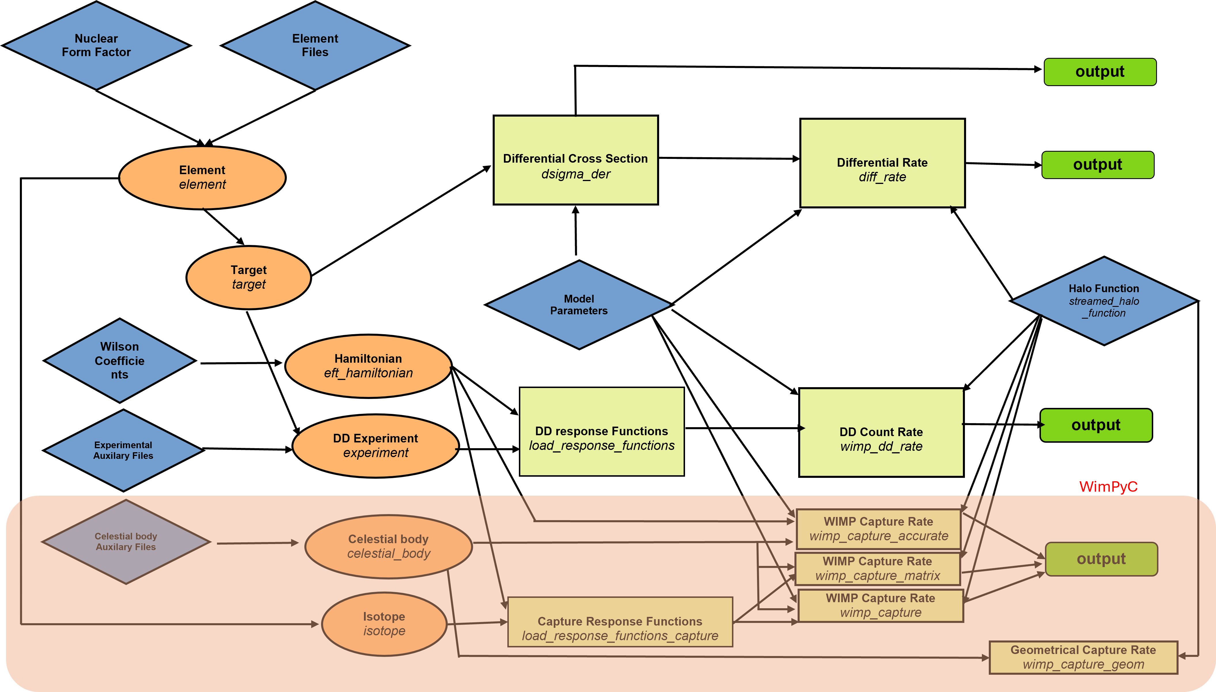
Figure 1: Main combined structure of WimPyDD and WimPyC (the shaded area includes the main components of the new module). Diamond–shaped elements indicate the input from the user, oval shapes contain classes and rectangles represent functions.

The structure of the code is summarized in Fig. 1. In such figure the shaded area contains the new classes and routines added by WimPyC, with diamond–shaped elements indicating the input from the user, classes are represented by oval shapes and functions by rectangles. In particular, the calculation of $C_{opt}$ requires to initialize a celestial body object through the class celestial_body, and makes use of a new class isotope, directly derived from the element class already existing in WimPyDD. The halo function information used in the calculation of $C_{opt}$ or $C_{geom}$ is the same used by WimPyDD to calculate DD signals.

3.1 Installation

To install the latest version of WimPyDD, including WimPyC, type:

                  git clone https://phab.hepforge.org/source/WimPyDD.git              

in the working directory, or download the code from WimPyDD’s homepage. This will create the folder WimPyDD, that, starting from version 2.0.0, includes a WimPyC subfolder. All the libraries required by the code are standard, such as matplotlib, numpy, scipy and pickle. A joint import of the functions and classes of both WimPyDD and WimPyC is obtained by typing something like:

                  import WimPyDD as WD              

3.2 New routines

We introduce in this Section the new routines of the WimPyC module. They work in the same way of those already existing in WimPyDD, taking some of the same inputs and assuming the same default values for them. In particular, in this and in the following sections we will only describe the features not already present in the original WimPyDD distribution, and address the reader to Ref. [1] for the others.

To calculate the WIMP capture rate $C_{opt}$ in the optically thin limit (in s^-1) of Eq. (2.2) with the expression of Eq. (LABEL:eq:capture_master) use:

                  WD.wimp_capture(celestial_body_obj, hamiltonian, vmin, delta_eta,        mchi,**args)              

with celestial_body_obj an object that defines the celestial body (see Section 3.3.1), mchi the WIMP mass $m_{\chi}$ in GeV, vmin and delta_eta two arrays in km/s and (km/s)^-1, respectively, containing the $u_{k}$ and $\delta\eta_{k}$ quantities for the halo function defined in Eq. (2.20) (WimPyDD provides the routine streamed_halo_function to calculate them, see Appendix E of Ref. [1]) and hamiltonian defines the effective Hamiltonian of Eq. (2.8) (initialized following the instructions provided in Section 3.3.3 of [1]). If present, the arguments $x_{i}$ of the Wilson coefficients $c_{j}^{\tau}$ are passed by **args. For all the other inputs and their default values (such as the WIMP local density $\rho_{\chi}$, the mass splitting $\delta$, etc.) check the Python prompt help (when applicable, they are the same as, for instance, in the wimp_dd_rate routine for direct detection). The matrix ${\cal M}$ of Eq. (2.21) can be obtained by using:

                  M=WD.wimp_capture_matrix(celestial_body_obj, hamiltonian, vmin,        delta_eta, mchi, **args)              

The output matrix M returned by wimp_capture_matrix is in the isospin basis $c=\{c_{j}^{\tau}\}$. A dictionary containing the correspondence between the matrix indices and the couplings can be obtained using:

                  WD.get_mapping(hamiltonian)              

The matrix M can be rotated into a new matrix M_pn in the proton-neutron basis $c=\{c_{j}^{(p,n)}\}$ using

                  U=WD.rotation_from_isospin_to_pn(hamiltonian)        M_pn=np.dot(U.T,npdot(M,U))              

A dictionary with the mapping between the indices of M_pn and the couplings $c_{i}^{(p,n)}$ is obtained using:

                  WD.get_mapping(hamiltonian, pn=True)              

In order to speed-up the calculations the wimp_capture and wimp_capture_matrix routines interpolate the response functions defined in Eq. (2.17). This approach drastically reduces the computational time compared to a full integration, and we have verified its accuracy at the percent level in a very extensive class of cases (for different celestial bodies, momentum and velocity suppressed interactions, inelastic scattering, massless mediator). However, for completeness and validation porpuses the WimPyC distribution includes the routine WD.wimp_capture_accurate that performs the calculation without approximations. In particular, for each value of the distance $r$ from the center of the celestial body and of the asymptotic velocity $u$ such routine obtains a single function of the recoil energy performing all the sums appearing in Eq. (LABEL:eq:capture_master) (i.e. summing over the couplings combinations, the nuclear isospin and the index $a=0,1,1E,1E^{-1}$) before calculating explicitly the energy integrals from $E_{1}(u,r)$ to $E_{2}(u,r)$. By avoiding interpolations and by inverting energy integrations and linear combinations this procedure allows to verify the level of accuracy of the wimp_capture and wimp_capture_matrix routines, also in the case of large cancellations among the different terms in the sums of Eq. (LABEL:eq:capture_master). To use it, type:

                  WD.wimp_capture_accurate(celestial_body_obj, hamiltonian, vmin,        delta_eta, mchi,**args)              

The WD.wimp_capture_accurate routine is significantly slower than wimp_capture and is supposed to be used for validating purposes. One can limit its scope using arguments such as $\verb|targets_list|$, tau_range, tau_prime_range and n_vel_list to include in the sums only some targets, some values of $\tau$ and $\tau^{\prime}$ and of the index $a$ of Eq. (2.17).

Finally, the geometrical capture rate of Eq. (2.25) can be calculated using:

                  WD.wimp_capture_geom(celestial_body_obj,mchi,vmin,delta_eta,        rho_loc=0.3)              

An example of the output of the wimp_capture_geom routine is represented by the horizontal line in the bottom plot of Fig. 5.

3.3 New classes

3.3.1 Celestial body

Main attributes: mass (mass in solar masses), name (string with name), r_vec (array with radius sampling, normalized to the interval $0-1$), rho_tot (array with the total density radial profile $\rho_{tot}(r)$ tabulated over r_vec), radius (radius in solar radii), mass_fractions (dictionary of total mass fractions $f_{i}$ of different targets), rho_i (dictionary returning for each target the density profile $\rho_{i}(r)$ normalized to the total mass fraction, target_names (list of strings containing the names of the targets in the celestial body - corresponds to the keys of the dictionaries mass_fractions and rho_i ), targets (list of isotope objects defining the targets, v_esc (array with the escape velocity as a function of the radius) and T_c (core temperature in Kelvin, used by the wimp_annihilation routine, see Appendix C).

The input of the class is a string with the name of the celestial body that corresponds to a folder containing the required information:

                  sun=WD.celestial_body(’Sun’)
              

In the example above all the information about the Sun is loaded from the folder WimPyDD/Wimp_Capture/Celestial_bodies/Sun (details on how to initialize such directory are provided in Section 4).

For instance:

                  integrate.simps(4*np.pi*sun.r_vec**2*sun.rho_tot,sun.r_vec)
        1.00
        sun.mass
        1.0
        integrate.simps(4*np.pi*earth.r_vec**2*earth.rho_tot,earth.r_vec)
        1.00
        integrate.simps(4*np.pi*sun.r_vec**2*sun.rho_i[’4He’],sun.r_vec)
        0.2519423743466878
        sun.mass_fractions[’4He’]
        0.2519423743466878
        earth=WD.celestial_body(’Earth’)
        earth.mass
        3.002732577e-06
        integrate.simps(4*np.pi*earth.r_vec**2*earth.rho_i[’28Si’],
        earth.r_vec)
        0.14402598587242832
        earth.mass_fractions[’28Si’]
        0.14402598587242832
              

3.3.2 Isotope

                  WD.isotope(symbol, element=None, verbose=True)              

Main attributes: symbol (string with formula of isotope), element (optional, WimPyDD element object containing the isotope information), mass (isotope mass), spin (isotope spin), z (atomic number), a (mass number), func_w (nuclear form factors),
diff_response_functions_capture and response_functions_capture(differential and integrated response functions for the calculation of the WIMP capture rate).

At instantiation the isotope class extracts the information about the isotope from an element object that contains it. In particular, if the element argument is not passed the class initializes it using the information contained in the folder WimPyDD/Targets. For instance, with the following input:

                  si28=WD.isotope(’28Si’)              

the isotope class strips the string ’28Si’ of the leading digits, initializes internally an element object issuing the command element_object=WD.element(’Si’) (that is successful if the file Si.tab is present in the folder WimPyDD/Targets) and looks for the string ’28Si’ in the element_object.isotopes attribute in order to extract the relevant information. The nuclear response functions necessary for the calculation of the WIMP–nucleus scattering process and taken from [3, 27] are available in WimPyDD for 22 default elements (see [1]) that can be listed issuing the command:

                  WD.list_elements()              

So, in order to add a new isotope it is necessary to initialize first an element containing it in the WimPyDD/Targets directory. The procedure to add new elements with the corresponding nuclear form factors, or to use alternative nuclear form factors for existing targets is provided in Appendix D of Ref. [1]. WimPyC comes with a set of pre–defined isotopes that can be listed by issuing:

                  WD.list_isotopes()        Available isotope objects in WimPyDD:        import WimPyDD as WD        WD.C12 WD.C13 WD.N14 WD.N15 WD.O16 WD.O17 WD.O18 WD.H1 WD.Ne20        WD.Na23 WD.Mg24 WD.Al27 WD.Si28 WD.P31 WD.S32 WD.He3 WD.Ar40        WD.Ca40 WD.He4 WD.Fe56 WD.Ni58        Use print() to get info on each isotope. For instance:        Type print(WD.Fe56)        symbol 56Fe, atomic number 26, mass 52.136        Nuclear form factor:Definition from Phys.Rev.C 89 (2014) 6,        065501 (e-Print: 1308.6288[hep-ph]) used        for nuclear W functions as default              

3.4 Response functions for capture

Given the effective Hamiltonian eft_hamiltonian_obj and the target $T$ = isotope_obj the differential response functions $\left[\frac{d\tilde{\sigma}_{T}^{a}}{dE_{R}}\right]_{jk}^{\tau\tau^{\prime}}(E_{R})$ defined in Eq. (2.16) and the tabulated values of the functions $\left[\bar{\sigma}^{a}_{T}\right]_{jk}^{\tau\tau^{\prime}}(E_{R})$ ($a=0,1,1E,1E^{-1}$) of Eq. (2.17) are loaded by the routine:

                  WD.load_response_functions_capture(input_obj, hamiltonian,
        j_chi=0.5)              

where the WIMP spin j_chi is set to 1/2 by default. input_obj can either belong to the isotope class or to the celestial_body class (in the latter case the response functions are loaded for all the targets in the celestial body). The differential and integrated response functions are loaded in the diff_response_functions_capture and response_functions_capture attributes of isotope objects, which are empty dictionaries when the isotope is initialized. In particular, the instructions:

                  c12_15=WD.eft_hamiltonian(’c12_15’,{12: lambda: [1,1],
        15: lambda: [1,1]})
        Al27=WD.isotope(’27Al’)
        j_chi=0.5
        WD.load_response_functions_capture(Al27,c12_15,j_chi=0.5)
        tau=0
        tau_prime=0
        c12_15.coeff_squared_list
        [(12, 12), (12, 15), (15, 12), (15, 15)]
        ij=1
        ci,cj=c12_15.coeff_squared_list[ij]
        n_vel=2 # 0,1,1E, 1Em1        dsigma_der=Al27.diff_response_functions_capture[’c12_15’,j_chi,
        ci,cj][tau,tau_prime,n_vel]
        E_R,sigma_bar=Al27.response_functions_capture[’c12_15’, j_chi][ij]
        [n_vel][tau][tau_prime]              

initialize an effective Hamiltonian $c_{12}{\cal O}_{12}+c_{15}{\cal O}_{15}$, the differential response function $\left[\frac{d\tilde{\sigma}_{{}^{27}Al}^{1E}}{dE_{R}}\right]_{12,15}^{\tau\tau^{\prime}}(E_{R})$, and the two arrays E_R and sigma_bar that tabulate the integrated response function $\left[\bar{\sigma}^{1E}_{{}^{27}Al}\right]_{12,15}^{00}(E_{R})$ as a function of the recoil energy. In both cases the $(i,j)=(12,15)$ coupling combination is set by the index ij=1, of one of the entries of the
eft_hamiltonian_obj.coeff_squared_list attribute, while n_vel=2 identifies $1E$ in the list $(0,1,1E,1E^{-1})$.

In the example above the E_R and sigma_bar tabulated values are read from the file 27Al_c_12_c_15.npy contained in WimPyDD/WIMP_Capture/Response_functions/spin_1_2/ folder. If such file does not exist it is created and the integrals of Eq. (2.17) are calculated and saved in it. The convention for the file names is identical to the case of DD case, see Section 3.4 of [1] (“Handling the response functions set”) for a detailed discussion. In particular, a different file is saved for each of the coupling combinations listed in the coeff_squared_list attribute of the eft_hamiltonian object. Notice that the $\bar{\sigma}$ functions are attributes of the isotope objects, and not of the celestial_body objects. This implies that the same file is read for a given isotope, irrespective on the celestial body where it is contained.

The distribution of WimPyC includes a set a of tabulated functions that reproduce all the examples listed in Section 4 and on the code website wimpydd.hepforge.org. By default the routine tabulates $\left[\bar{\sigma}^{a}_{T}\right]_{jk}^{\tau\tau^{\prime}}(E_{R})$ for 1000 values of the integration upper bound $E_{R}$ (the number of sampled points and the minimal and maximal values of $E_{R}$ can be changed using the arguments n_sampling and er_min_cut, er_max_cut).

The response functions provided by default in the WimPyC distribution have been extensively tested to verify that their sampling is accurate enough in a very wide range of cases, including inelastic scattering, a massless propagator, interference among different interaction operators, etc. Nevertheless, the parameter space of WIMP capture is particularly extended, with very different kinematic regimes across different celestial bodies, nuclear targets and interactions types. As a consequence, in Appendix D we provide a discussion of this aspect, showing how the user can easily check possible under–sampling issues that may arise in particular corners of the parameter space. In case of need, the sampling of the response functions can be increased by passing to the load_response_functions_capture routine an array of energy values er_sampling in keV. Moreover, setting increase_sampling=True overwrites existing tabulated functions including the additional points, while force_recalculation=True recalculates them from scratch. The array er_sampling can be provided independently by the user or obtained for the object target belonging to the isotope class using:

                  er_sampling=        WD.get_wimp_capture_response_functions_energy_sampling(target,
        celestial_body_list, mchi_list,delta_list,vmin, n_sampling=1000)              

where celestial_body_list contains a list of celestial_body objects, mchi_list contains a list of $m_{\chi}$ values, delta_list a list of $\delta$ values, vmin an array with values of the WIMP asymptotic speed $u$, and n_sampling fixes the length of the returned array, whose energy values are tuned on the input parameters by calculating a sample of the $E_{1}$, $E_{2}$ energies of Eq. (2.3).

4 Examples of capture rate calculations

In the following, we provide a few examples for the calculation of the WIMP capture rate. They use implementations of the celestial bodies that are included in the distribution of WimPyC. To get their list type:

                  WD.list_celestial_bodies()        WD.Sun WD.Earth WD.Jupiter WD.White_Dwarf WD.MS_Star
              

See appendix B for some details about their implementation.

4.1 Sun, NREFT operators

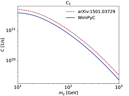
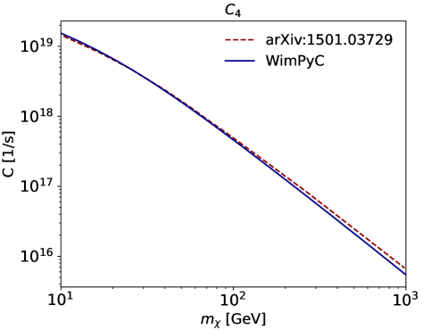
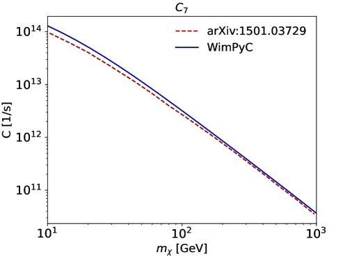
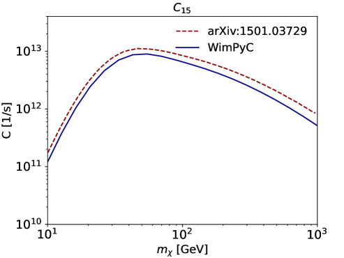
Figure 2: The WimPyC capture rate for the Sun, using the selected NREFT operators, is compared with the results of Ref. [27].

In the example below the capture rate in the Sun is calculated for the ${\cal O}_{1}$, ${\cal O}_{4}$, ${\cal O}_{7}$ and ${\cal O}_{15}$ operators of the effective Hamiltonian of Eq. (2.8). In all cases an isoscalar interaction with $c^{0}=10^{-3}/m_{v}^{2}$, $m_{v}$ = 246.2 GeV, $c^{1}$ = 0 is adopted, as well as a standard Maxwellian velocity distribution with $\rho_{\chi}=0.4$ GeV/cm³. In Fig. 2 the output is compared to the results of Ref. [27].

                  vmin,delta_eta=WD.streamed_halo_function(v_esc_gal=550)        mchi_vec=np.logspace(1, 3, 50)        ### repeat for NREFT operators (1, 4, 7, 15)        c7 = WD.eft_hamiltonian(’c7’, {7 : lambda c0, c1:        np.array([c0, c1])})        mv=246.2        capture=[WD.wimp_capture(WD.Sun, c7, vmin, delta_eta, mchi,
        rho_loc=0.4, c0=1e-3/mv**2, c1=0) for mchi in mchi_vec]              

4.2 Sun, SI interaction, inelastic scattering

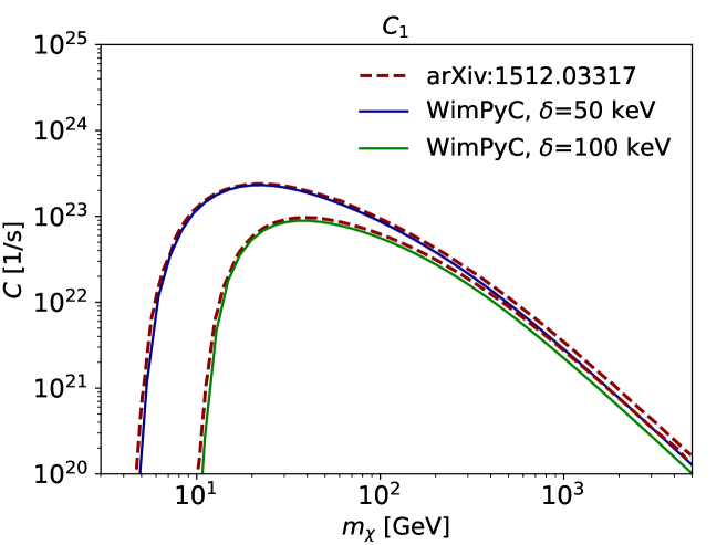
Figure 3: The WimPyC capture rate for the Sun in the inelastic scenario is compared with published results [39], considering $\sigma_{\chi{\cal N}}=10^{-42}$ cm² for a spin-independent interaction.

In this example an isoscalar SI interaction (${\cal O}_{1}$ effective operator) is parameterized in terms of the WIMP–nucleon cross section, $\sigma_{\chi{\cal N}}$ = $(c^{\cal N})^{2}\mu_{\chi{\cal N}}^{2}/\pi$, with ${\cal N}$ = proton, neutron, $1/\mu_{\chi,{\cal N}}=1/m_{\chi}+1/m_{\cal N}$. WimPyDD implements the Wilson coefficients $c_{1}^{0}$, $c_{1}^{1}$ in terms of $\sigma_{\chi{\cal N}}$ using the function:

                  WD.c_tau_SI(sigma_p, mchi, cn_over_cp=1)              

with cn_over_cp the ratio $c_{1}^{n}/c_{1}^{p}$ between the WIMP–neutron and the WIMP–proton couplings (see Ref. [1] and online help). The output for inelastic scattering is obtained passing to WD.wimp_capture a non–vanishing value of the delta parameter in keV. In Fig. 3 the result for $\sigma_{\chi{\cal N}}$ = $10^{-42}$cm², and $\delta$ = 50, 100 keV is compared to that of Ref. [39], considering an isoscalar interaction (for details of how to tune the halo function using the WD.streamed_halo_function routine see Appendix E of [1]).

                  vmin,delta_eta=WD.streamed_halo_function(v_esc_gal=544)
        mchi_vec=np.logspace(np.log10(4), np.log10(5000), 50)        SI=WD.eft_hamiltonian(’SI’,{1: WD.c_tau_SI})
        ### repeat for delta=50, 100        delta=50        capture=[WD.wimp_capture(WD.Sun, SI, vmin, delta_eta, mchi,        delta, rho_loc=0.4, sigma_p=1e-42) for mchi in mchi_vec]              

4.3 Earth, NREFT operators

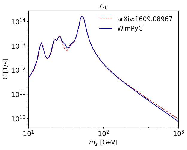
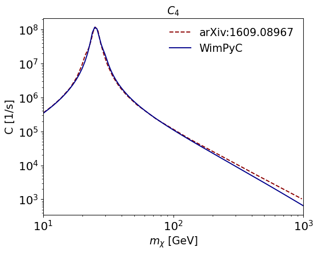
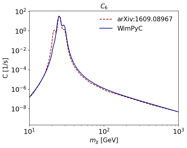
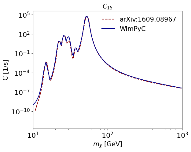
Figure 4: The WimPyC capture rate for Earth, using the selected NREFT operators, is compared to the results of Ref. [40].

This example is analogous to that of Section 4.1, for the Earth. In Fig. 4 the output is compared to that of Ref. [40] for the NREFT operators ${\cal O}_{i}$, $i=1,4,6,15$.

                  vmin,delta_eta=WD.streamed_halo_function(v_esc_gal=533)
        mchi_vec=np.logspace(1, 3, 50)        ### repeat for NREFT operators (1, 4, 6, 15)        c6 = WD.eft_hamiltonian(’c6’,        { 6: lambda c0, c1: np.array([c0, c1])})
        mv=246.2        capture=[WD.wimp_capture(WD.Earth,c6,vmin,delta_eta, mchi,        rho_loc=0.4, c0=1e-3/mv**2, c1=0) for mchi in mchi_vec]              

4.4 Jupiter, SD interaction

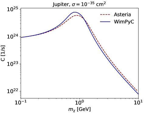
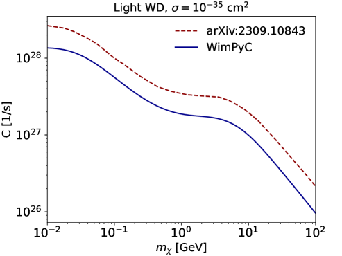
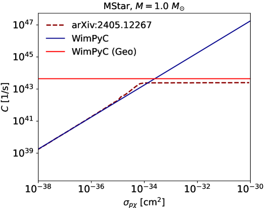
Figure 5: The capture rate calculated using WimPyC for Jupiter (top-left), a light WD (top-right), and a main sequence star (bottom) is compared with the results from Refs. [14], [41] and [42], respectively.

In the following example a standard SD interaction (corresponding to the ${\cal O}_{4}$ operator) is parameterized in terms of the corresponding WIMP–proton cross section $\sigma_{\chi p}$ implemented by the WD.c_tau_SD routine (which is the analogous of WD.c_tau_SI for a SD interaction). In the top-left panel of Fig. 5 the WimPyC output for Jupiter, $\sigma_{\chi p}=10^{-35}$cm² and a standard Maxwellian velocity distribution is compared with the result of Refs. [14, 43].

                  vmin,delta_eta=WD.streamed_halo_function(v_esc_gal=550)
        mchi_vec=np.logspace(np.log10(1e-1), np.log10(10), 50)        SD=WD.eft_hamiltonian(’SD’, {4: WD.c_tau_SD})
        capture=[WD.wimp_capture(WD.Jupiter, SD, vmin, delta_eta, mchi,        rho_loc=0.4, sigma_p=1e-35, cn_over_cp=0) for mchi in mchi_vec]              

4.5 White Dwarf close to Galactic Center, SI interaction

In the example below, a White Dwarf close to the Galactic center is considered, following Ref. [41], with parameters: $\rho_{\chi}\simeq$ 9322.7 GeV cm³, and a Maxwellian distribution where the escape velocity is neglected. The velocity dispersion is $v_{rms}$ = 270 km/s, and the velocity of the White Dwarf in the Galactic rest frame is $\vec{v}_{rot,Gal}$ = 285 km/s.

                  ##the escape velocity is neglected, v_esc_gal set to large number        vmin, delta_eta=WD.streamed_halo_function(v_rot_gal=        np.array([ 0., 285., 0.]), v_sun_rot=np.array([ 0., 0., 0.]),        v_esc_gal=10000, vrms=270)        mchi_vec=np.logspace(np.log10(1e-2), np.log10(100), 50)        model=WD.eft_hamiltonian(’SI’,{ 1: WD.c_tau_SI})        capture=[WD.wimp_capture(WD.White_Dwarf, model,vmin, delta_eta,        mchi, rho_loc=9322.7, sigma_p=1e-35) for mchi in mchi_vec]              

In the top-right panel of Fig. 5 the capture rate calculated using WimPyC is compared with the published results from Ref. [41].

4.6 Main Sequence star, SI interaction, geometric limit

In the following example WD.MS_Star represents a main sequence star with mass and radius of the Sun and 100% Hydrogen composition close to the Galactic Center.

                  vmin,delta_eta=        WD.streamed_halo_function(v_rot_gal=np.array([0.,1000.,0.]),        v_esc_gal=550)        sigma_p_vec=np.logspace(np.log10(1e-39), np.log10(1e-30), 50)        SI=WD.eft_hamiltonian(’SI’,{ 1: WD.c_tau_SI})        capture=[WD.wimp_capture(WD.MS_Star, SI,vmin, delta_eta,        mchi=0.1, rho_loc=2e12, sigma_p=sigma_p)
        for sigma_p in sigma_p_vec]        c_geom=WD.wimp_capture_geom(WD.MS_Star, mchi=0.1, vmin=vmin,
        delta_eta=delta_eta, rho_loc=2e12)              

In the bottom plot of Fig. 5 the WimPyDD result for the capture rate is plotted as a function of the WIMP–nucleon scattering cross section and compared to that of Ref. [42] for a SI interaction, $m_{\chi}$ = 0.1 GeV, $\rho_{\chi}$ =2$\times 10^{12}$ GeV cm^-3 and an orbital velocity of 1000 km/s. In the same plot the horizontal solid line represents the geometric capture rate calculated by wimp_capture_geom. In such plot one can observe the transition from the optically thin to the optically thick regime, and how in WimPyC the more refined treatment of Ref. [42] can be reproduced reasonably well by interpolating between the optically thin result and the geometric limit.

4.7 Matching of non–relativistic Wilson coefficients: anapole DM

The completeness of the base of the NREFT Hamiltonian of Eq. (2.8) implies that WimPyC can be used to calculate the capture rate for any high–energy physics interaction between the WIMP and the nucleus, once the low–energy Wilson coefficients are properly matched. We exemplify this procedure in the specific example of a DM particle that interacts with ordinary matter entirely through an electromagnetic anapole moment [44, 45]. The interaction Lagrangian is given by:

$${\cal L}=\frac{1}{2}\frac{g}{\Lambda^{2}}\,\bar{\chi}\gamma^{\mu}\gamma^{5}\chi\,\partial^{\nu}F_{\mu\nu},$$ (4.1)

where $\chi$ is the Anapole DM (ADM) field, $F_{\mu\nu}$ is the electromagnetic field strength tensor, $g$ is a dimensionless coupling constant, and $\Lambda$ is a new physics scale. The nonrelativistic scattering of an ADM particle with a nucleon can also be described by the contact interaction Hamiltonian

$$H_{\chi N}=\frac{2eg}{\Lambda^{2}}\,\vec{S}_{\chi}\cdot\bigg(e_{N}\vec{v}_{\chi N}^{\perp}+i\frac{(g_{N}/2)}{m_{N}}\,\vec{q}\times\vec{S}_{N}\bigg).$$ (4.2)

In the equation above $e$ is the elementary electric charge, $e_{N}$ is the nucleon charge in units of $e$ ($e_{\rm p}=1$, $e_{\rm n}=0$), $g_{N}/2$ is the nucleon magnetic moment in units of nuclear magnetons $e/2m_{N}$ ($g_{\rm p}=5.585\,694\,713(46)$, $g_{\rm n}=-3.826\,085\,45(90)$), $m_{N}$ is the nucleon mass, $\vec{S}_{\chi}$ and $\vec{S}_{N}$ are the spins of the WIMP and the nucleon, respectively, $\vec{q}$ is the momentum transfer, and $\vec{v}^{\perp}_{\chi N}$ is the component of the WIMP–nucleon relative velocity perpendicular to $\vec{q}$. In the base of Ref. [2] Eq. (4.2) reads:

$$H_{\chi N}=\sum_{\tau=0,1}(c_{8}^{\tau}{\cal O}_{8}+c_{9}^{\tau}{\cal O}_{9})t^{\tau},$$ (4.3)

with the $c_{8}^{\tau}$ and $c_{9}^{\tau}$ Wison coefficients given by:

$$c_{8}^{\tau}=\frac{2eg}{\Lambda^{2}}\,e^{\tau},\qquad c_{9}^{\tau}=-\frac{eg}{\Lambda^{2}}\,g^{\tau},$$ (4.4)

and $e^{0}=e^{1}=1$, $g^{0}=g_{\rm p}+g_{\rm n}$, $g^{1}=g_{\rm p}-g_{\rm n}$. In particular, the low–energy phenomenology depends on the WIMP mass $m_{\chi}$ and on the reference cross section:

$$\sigma_{\rm ref}\equiv\frac{2\mu_{\chi{\cal N}}^{2}\,\alpha g^{2}}{\Lambda^{4}}\,,$$ (4.5)

where $\alpha=e^{2}/4\pi\simeq 1/137$ is the fine structure constant and $\mu_{\chi{\cal N}}$ the WIMP–nucelon reduced mass. The implementation of the model in WimPyC is straightforward, and requires to define two functions c8_anapole(mchi,sigma_ref) and c9_anapole(mchi,sigma_ref) returning as a function of $m_{\chi}$ and $\sigma_{\rm ref}$ the 2–dimensional arrays $\left[c_{8}^{0},c_{8}^{1}\right]$ and $\left[c_{9}^{0},c_{9}^{1}\right]$ containing the isoscalar and isovector components of the Wilson coefficients in units of GeV^-2. Explicitly:

                  def c8_anapole(mchi,sigma_ref):         hbarc=1.972e-14 #hbar*c in GeV*cm         e_tau=np.array([1,1])         m_N=0.931 #nucleon mass in GeV         m_chi_N=mchi*m_N/(mchi+m_N)         eg_over_lambda2=np.sqrt(2*np.pi*sigma_ref)/(m_chi_N*hbarc)         return 2*eg_over_lambda2*e_tau                def c9_anapole(mchi,sigma_ref):         hbarc=1.972e-14 #hbar*c in GeV*cm         gp=5.585694713         gn=-3.82608545         g_tau=np.array([gp+gn,gp-gn])         m_N=0.931 #nucleon mass in GeV         m_chi_N=mchi*m_N/(mchi+m_N)         eg_over_lambda2=np.sqrt(2*np.pi*sigma_ref)/(m_chi_N*hbarc)         return -eg_over_lambda2*g_tau                wilson_coeff_anapole={8: c8_anapole, 9: c9_anapole}        anapole=WD.eft_hamiltonian(’anapole’, wilson_coeff_anapole)              

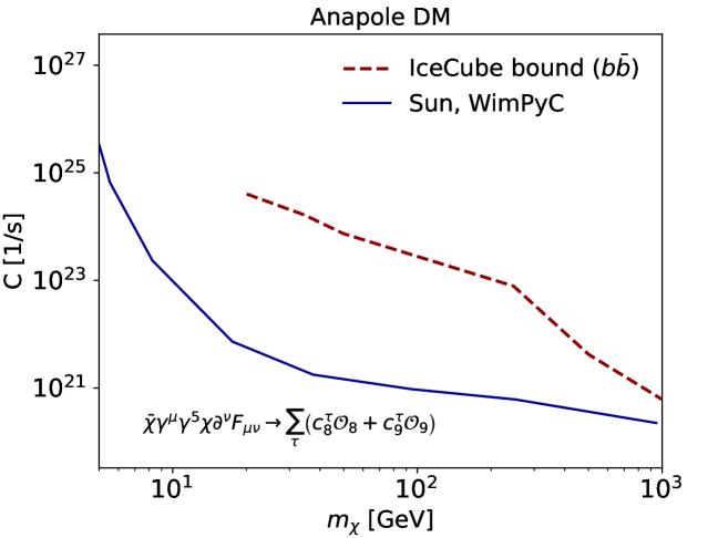
Figure 6: Maximal capture rate in the Sun for Anapole DM allowed by the DD exclusion plot of Ref. [46] compared to the IceCube upper bound [47] assuming $b\bar{b}$ annihilation

.

The largest ADM capture $C_{\odot}$ in the Sun allowed by DD can be obtained by calculating it over the exclusion plot of $\sigma_{\rm ref}$ vs. $m_{\chi}$ provided in Fig.2 of Ref. [46]. In Fig. 6 the corresponding output of wimp_capture is compared to the upper bound on the annihilation rate $\Gamma_{\odot}$ for the $b\bar{b}$ channel [47] (see instance, Fig.5 of [12])).

                  # mchi and sigma_ref from exclusion plot of 1808.04112        mchi_lim=np.array([4.35,4.60,5.54,8.26,17.52,37.49,94.80,251.07,        945.86])        sigma_ref_lim=np.array([2.36e-34, 1.91e-35, 1.10e-36, 4.92e-38,        2.54e-39, 1.20e-39, 1.81e-39, 4.29e-39,1.42e-38])        vmin, delta_eta=WD.streamed_halo_function() #standard Maxwellian        #calculation of ADM capture rate in the Sun        capture_vec=np.array([])        for mchi,sigma_ref in zip(mchi_lim,sigma_ref_lim):         capture=WD.wimp_capture(WD.Sun, anapole,         vmin,delta_eta, mchi,sigma_ref=sigma_ref)         capture_vec=np.append(capture_vec,capture)        #check equilibrium between capture and annihilation        annihilation_vec=np.array([])        for mchi,capture in zip(mchi_lim,capture_vec):         annihilation=WD.wimp_capture_annihilation(WD.Sun,mchi,capture)         annihilation_vec=np.append(annihilation_vec,annihilation)        print(capture_vec/(2*annihilation_vec))        [1. 1. 1. 1. 1. 1. 1. 1. 1.]              As shown at the bottom of the example, using the wimp_capture_annihilation routine (see Appendix C) one can numerically verify that the equilibrium condition $\Gamma_{\odot}=C_{\odot}/2$ holds in the full range of $m_{\chi}$ (when the default value $\langle\sigma v\rangle$ = 3$\times$ 10^-26 cm³ s^-1 is used for the WIMP annihilation cross section times velocity).

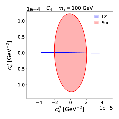
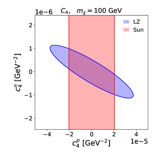
Figure 7: $90\%$ C.L. allowed region in the $c^{p}\times c^{n}$ plane for the DD experiment LZ [48], and considering capture inside the Sun while assuming $b\bar{b}$ annihilation for the IceCube upper bound [47]. The left panel corresponds to the $\mathcal{O}_{4}$ (standard SD) interaction, while the right panel is its zoomed-in version.

4.8 Matrix in couplings space for the calculation of the capture rate

The effective couplings of the Anapole model of the previous example lie in the four–dimensional vector space $c=(c_{8}^{0},c_{8}^{1},c_{9}^{0},c_{9}^{1})$. For a specific value of the WIMP mass mchi the corresponding matrix ${\cal M}$ can be obtained using wimp_capture_matrix. In such case an auxiliary effective Hamiltonian with all couplings fixed to unity needs to be defined (values different from unity can be used, if a different normalization of the couplings and of the matrix elements is needed). Notice that the class eft_hamiltonian always expects that the Wilson coefficient is a function, so in this case the routine with no arguments lambda: [1,1] is used to parameterize constant coefficients.

                  # auxiliary model needed by wimp_capture_matrix        wilson_coeff_aux=        {k:lambda:[1,1] for k in wilson_coeff_anapole.keys()}        anapole_aux=WD.eft_hamiltonian(’anapole_aux’,wilson_coeff_aux)        # use mchi_lim[6]=94.8 from previous example        matrix=WD.wimp_capture_matrix(WD.Sun,anapole_aux,vmin,delta_eta,        mchi_lim[6])        matrix.shape        (4, 4)        #mapping between couplings and positions in the matrix        WD.get_mapping(anapole_aux)        (8, 0): 0, (8, 1): 1, (9, 0): 2, (9, 1): 3        #couplings vector using sigma_ref_lim[6]=1.81e-39        c_vec=np.append(c8_anapole(mchi_lim[6],sigma_ref_lim[6]),        c9_anapole(mchi_lim[6],sigma_ref_lim[6]))        [1.17426826e-05,1.17426826e-05,-1.03312665e-05,-5.52597735e-05]        # capture rate        capture_matrix=np.dot(c_vec,np.dot(matrix,c_vec))        9.490518349177376e+20              

The capture rate calculated in this way matches the output of wimp_capture in the previous example.

In particular, as shown in Ref. [21], the complementarity of DD experiments and WIMP capture in the Sun can be studied using the matrix-based formalism, where the parameter space allowed by each experiment $exp$ lies inside the ellipsoid $c^{T}\cdot{\cal M}_{exp}\cdot c<R_{exp}^{max}$, with $R_{exp}^{max}$ the corresponding experimental upper bound. In Fig. 7, we compare the latest results of the LZ experiment [48] with the IceCube upper bound assuming $b\bar{b}$ annihilation [47], by plotting the allowed parameter space for each experiment in the $c^{p}\times c^{n}$ plane for $m_{\chi}=100$ GeV, assuming $\mathcal{O}_{4}$ interaction. The explicit implementation of the relevant matrices, which also makes use of the wimp_dd_matrix routine for DD, corresponds to:

                  vmin,delta_eta=WD.streamed_halo_function()        c4=WD.eft_hamiltonian(’c4’,{4: lambda: [1,1]})        U_pn= WD.rotation_from_isospin_to_pn(model)        matrix_Sun = WD.wimp_capture_matrix(WD.Sun, c4, vmin, delta_eta,        mchi=100)        matrix_Sun_pn = np.dot(U_pn, np.dot(matrix_Sun, U_pn))        LZ=WD.experiment(’LZ_2022’)        matrix_LZ=WD.wimp_dd_matrix(LZ,c4,0,vmin,delta_eta, mchi=100)        matrix_LZ_pn = np.dot(U_pn, np.dot(matrix_Sun, U_pn))              Notice that the output of both wimp_capture_matrix and wimp_dd_matrix is in isospin space and needs to be rotated into the $(p,n)$ space using the output of
rotation_from_isospin_to_pn.

4.9 Halo–independent methods

The routine wimp_capture takes as inputs the arrays vmin, delta_eta containing the halo function and returns the capture rate by summing the master formula of Eq. (LABEL:eq:capture_master) over the velocity streams contained in vmin, delta_eta. To control this behavior wimp_capture has the argument sum_over_streams with default value True. If, instead, sum_over_streams=False the sum over the velocity streams is not performed and wimp_capture returns an array with shape vmin.shape (in particular wimp_capture accepts any shape for vmin and delta_eta, allowing to sample a large number of stream sets efficiently with a single call).

This feature allows to calculate the response function ${\cal H}_{C}(u)$ defined in Eq. (2.23). In particular ${\cal H}_{C}(u_{k})$ can be factored out from the capture rate (see Eq. (2.22)) by setting $\lambda_{k}=\delta\eta_{k}u_{k}=1$, i.e. $\delta\eta_{k}=1/u_{k}$:

                  u=np.logspace(-3, np.log10(782), 1000)        h_c=WD.wimp_capture(WD.Sun, WD.SI, u, 1/u, mchi=40,        sum_over_streams=False,sigma_p=2.2e-48)        pl.plot(vmin,h_c)              

In the example above the WIMP LZ bound [48] on the WIMP–proton cross $\sigma_{p}$ for a SI interaction at $m_{\chi}$ =40 GeV (2.2$\times$ 10^-48 cm²) is used to calculate the response function ${\cal H}$ as a function of $u$. The output is shown in Fig. 8.

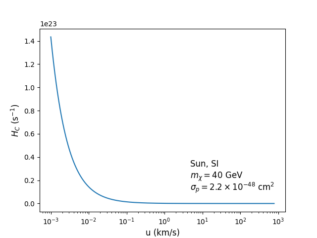
Figure 8: Response function ${\cal H}$ as a function of $u$ for a SI interaction and $m_{\chi}$ =40 GeV, $\sigma_{p}$ = 2.2$\times$ 10^-48 cm² (corresponding to the LZ upper bound from DD [49])

.

The way wimp_capture can be used for halo–independent methods to calculate the response function ${\cal H}_{C}(u)$ is identical to that of the wimp_dd_rate routine for DD, described in Sections 2.1 and 3.5.4 of [1].

4.10 Massless propagator

Since the Wilson coefficients of the effective Hamiltonian Eq. (2.8) are arbitrary functions of the transferred momentum $q$ in the functions passed to the eft_hamiltonian class the argument q is reserved for the transferred momentum $q$ in GeV. A common situation is when a momentum dependence is induced by a massless propagator. In this case the capture rate formally diverges, because it is driven by WIMPs locked on very large bound orbits with $q\rightarrow$ 0, where the WIMP–nucleus cross section diverges. A cut-off on the capture rate is usually obtained by assuming that the gravitational disturbances far from the Sun put an upper cut $r_{0}$ on the size of the maximal aphelion that a captured WIMP can have [50]. In particular, indicating with $R_{\odot}$ and $v_{esc}(R_{\odot})$ the Sun’s radius and the escape velocity from the Sun’s surface, a WIMP with initial position $r$ needs a minimal speed $v_{e}(r)^{2}=v_{esc}(r)^{2}-v_{esc}(r_{0})^{2}$ with $v_{esc}(r_{0})^{2}=v_{esc}(R_{\odot})^{2}R_{\odot}/r_{0}$ to reach the maximal distance $r_{0}$. In this case the expression of Eq. (2.5) for the minimal energy required for capture is modified to:

$$E^{\chi}_{\rm cap}(u)\rightarrow\frac{1}{2}m_{\chi}(u^{2}+v_{esc}(r_{0})^{2})-\delta$$ (4.6)

in order for the WIMP to be locked into a bound orbit with aphelion $r_{0}$. In the literature, $r_{0}$ is identified with the distance from the Sun to Jupiter [51, 52, 53], corresponding to:

$$v_{\rm esc}(r_{0})=v_{\rm cut}\simeq 18.5\,{\rm km/s}\,.$$ (4.7)

A non-vanishing value of $v_{\rm cut}$ increases $E^{\chi}_{\rm cap}$, making the condition for capture more stringent. It can be passed to the wimp_capture routine through the argument v_cut. Following Ref. [53], in the example below the Jupiter cut is applied for an isoscalar SI WIMP-nucleon interaction with $\sigma_{\rm ref}$ = $\sigma_{p}$ = $\sigma_{n}$= $c_{1}\mu^{2}_{\chi{\cal N}}/\pi\times F^{2}_{DM}(q)$ with $F_{DM}$ = $q_{0}/q$ or $(q_{0}/q)^{2}$ and $q_{0}$ = 0.1 GeV. In particular, the desired momentum–dependent Wilson coefficients can be obtained by multiplying the output of WD.c_tau_SI by $F^{2}_{DM}$. Also, the coupling 1 is modified to (1,’qm2’) for $F_{DM}$ = $q_{0}/q$ or (1,’qm4’) for $F_{DM}$ = $(q_{0}/q)^{2}$ in order to fix the name of the files where the response functions are saved. For instance, for Iron instead of 56Fe_c_1_c_1.npy, which contains the response functions for a contact interaction, the file name 56Fe_c_1_qm2_c_1_qm2.npy is used for $F_{DM}$ = $q_{0}/q$ and the file name 56Fe_c_1_qm4_c_1_qm4.npy is used for $F_{DM}$ = $(q_{0}/q)^{2}$ (a detailed discussion on how to handle the output files of different sets of response functions is provided in Section 3.4 of Ref. [1]).

                  # cn_over_cp = 1 for isoscalar interaction        c1_tau_SI_qm2=lambda sigma_p, mchi, q, cn_over_cp=1, q0=0.1:        WD.c1_tau_SI(sigma_p,mchi, cn_over_cp=1)*q0/q        c1_tau_SI_qm4=lambda sigma_p, mchi, q, cn_over_cp=1, q0=0.1:        WD.c1_tau_SI(sigma_p,mchi, cn_over_cp=1)*(q0/q)**2        model_qm2=WD.eft_hamiltonian(’F_DM_qm1’,{(1,’qm1’): c1_tau_SI_qm1}        model_qm4=WD.eft_hamiltonian(’F_DM_qm2’,{(1,’qm2’): c1_tau_SI_qm2}              

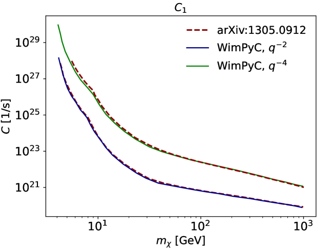
Figure 9: The output of WimPyC— for an isoscalar SI interaction modified by the momentum-dependent term $F_{DM}$ = $q_{0}/q$ or $(q_{0}/q)^{2}$ with $q_{0}$ = 0.1 GeV is compared to that of Ref. [53] when $m_{\chi}$ and $\sigma_{\rm ref}$ are taken from the corresponding exclusion plots in Fig.1 of the same paper.

Indicating with mchi and sigma_ref the WIMP mass $m_{\chi}$ and the reference cross section $\sigma_{\rm ref}$ the capture rate in the Sun, including the Jupiter cut, is then obtained using:

                  capture_qm2=WD.wimp_capture(WD.Sun, model_qm2, vmin, delta_eta,        mchi=mchi, sigma_p=sigma_ref, v_cut=18.5)        capture_qm4=WD.wimp_capture(WD.Sun, model_qm4, vmin, delta_eta,        mchi=mchi, sigma_p=sigma_ref, v_cut=18.5)              

In Fig. 9 the output of WimPyC is compared to that of Ref. [53] when $m_{\chi}$ and $\sigma_{\rm ref}$ are taken from the corresponding exclusion plots in Fig.1 of the same paper.

4.11 Differential capture

The capture rate of Eq. (LABEL:eq:capture_master) requires to perform the following radial integral, summed over the velocity streams $u_{k}$, the nuclear targets $T$ and each $c_{i}c_{j}$ combination of couplings in the effective Hamiltonian (Eq. (2.8)):

$$C_{opt}=\sum_{T}\sum_{ij}\sum_{k}\int_{0}^{R_{\odot}}d^{3}r\frac{dC^{T}_{ij}}{d^{3}rdu}(r,u_{k}).$$ (4.8)

In particular, $\frac{dC^{T}_{ij}}{d^{3}rdu}$ is related to the ${\cal H}_{C}$ function of Eq. (2.24):

$${\cal H}_{C}(u)=\frac{\rho_{\chi}}{m_{\chi}}\int_{0}^{R_{\odot}}4\pi r^{2}\sum_{T}\sum_{ij}\frac{1}{u}\frac{dC^{T}_{ij}}{d^{3}rdu}(r,u).$$ (4.9)

An array containing the values of $\frac{dC^{T}_{ij}}{d^{3}rdu}(r,u_{k})$ (in s^-1 cm^-3), tabulated over the r_vec values of the celestial_body object and the vmin array is accessible through the dynamic attribute dc_dvi that the routines wimp_capture and wimp_capture_accurate acquire after each call. dc_dvi is a python dictionary that accepts as key the symbol attribute of the target and one of the coupling combinations in the coeff_squared_list attribute of the interaction Hamiltonian. In the example below the WIMP LZ bounds [48] on the WIMP–proton cross $\sigma_{p}$ for a SI and SD interactions at $m_{\chi}$ =40 GeV (2.2$\times$ 10^-48 cm² and 9.8$\times$ 10^-42 cm², respectively) are used to calculate the corresponding capture rates in the Sun and the Earth, and the dynamic attribute dc_dvi is used to access the $\frac{dC^{T}_{ij}}{d^{3}rdu}(r,u_{k})$ values for the ${}^{56}Fe$ and the ${}^{27}Al$ targets. Notice that in this case the first value of the vmin array is equal to zero and is dropped from the sampling.

                  len(WD.Sun.r_vec)        135        vmin,delta_eta=WD.streamed_halo_function()        len(vmin)        1000        capture_SI=WD.wimp_capture(WD.Sun, WD.SI, vmin, delta_eta,        mchi=40, sigma_p=2.2e-48)        dc_dvi_SI=WD.wimp_capture.dc_dvi[’56Fe’,(1,1)]        dc_dvi_SI.shape        (135, 999)        capture_SD=WD.wimp_capture(WD.Sun, WD.SD, vmin, delta_eta,        mchi=40, sigma_p=9.8e-42)        dc_dvi_SD=WD.wimp_capture.dc_dvi[’27Al’,(4,4)]        dc_dvi_SD.shape        (135, 999)              

Appendix A Initializing the celestial body directory

Table 1: Files in the celestial body subfolder containing the information to calculate the capture rate.

Physical quantity(unit)	Default(if missing file)	File name
Mass (solar masses)	1	mass.tab
radius (solar radii)	1	radius.tab
density profiles	hydrogen sphere	densities.tab
(arbitrary units)	of constant density

Upon instantiation the celestial_body class reads the relevant information from a sub–folder of WimPyDD/WimPyC/Celestial_bodies. The name of the subfolder is passed as an argument to the celestial_body class. For instance, the instruction:

                  sun=WD.celestial_body(’Sun’)              

reads the files listed in Table 1 searching for them in the folder:

                  WimPyDD/WimPyC/Celestial_bodies/Sun              

The densities.tab file contains a table with the density profiles of the target elements in the celestial body.

                  # Solar density profiles from model AGSS09ph [arXiv.0909.2668]        r_vec rho_tot 1H 4He v_esc        0.0015 150.5 74.636 130.656
        0.0020 150.5 67.190 117.570
        0.0025 150.5 64.525 112.846
...
        ...
        ...              

In particular, as in the example above the file can start with a first optional line beginning with # containing documentation text that is added to the celestial_body_obj.__doc__ attribute of the celestial_body_obj object and printed out by the print(celestial_body_obj) command. The table content must be preceded by a line containing headers (without apostrophes) that allow WimPyC to identify the columns that follow. In particular the code looks for at least three headers: r_vec, corresponding to the radial distance from the center; rho_tot, corresponding to the total density profile; the valid symbol of at least one nuclear target (i.e. whose label must match one of the strings that identify a valid isotope object, and whose information is stored in the WimPyDD/Targets folder). In the numerical tables the units for the radial distance and for all the densities can be arbitrarily chosen, because, before loading them in the corresponding attributes of the celestial_body_obj, WimPyC rescales them using the information contained in the mass.tab and radius.tab files (which contain a single numerical value, besides an optional documentation line starting by #) so that $\int_{0}^{1}4\pi r^{2}\rho_{tot}(r)$=1 and $\int_{0}^{1}4\pi r^{2}\rho_{i}(r)$ = $f_{i}$. The only quantity in densities.tab that requires to be expressed in a specific unit is the escape velocity, corresponding to the v_esc header, that, if included in densities.tab, must be tabulated in km/s. If a column with header v_esc is initially not included WimPyC calculates it in km/s using the available information. In such case the user is prompted to add the new column with the tabulated escape velocity to the densities.tab file (this avoids to recalculate the escape velocity at every new instantiation).

For testing purposes and in order to provide a template folder that is easy to adapt to specific needs, WimPyC allows to instantiate a celestial body without initializing the corresponding folder in the WimPyDD/WimPyC/Celestial_bodies directory, or when the folder is empty. In particular, if the WimPyDD/WimPyC/Celestial_bodies/Template folder does not exist, the instruction:

                  template=WD.celestial_body(’Template’)
              creates it, with the three files mass.tab, radius.tab and densities.tab that initialize by default a hydrogen sphere of unit mass and unit radius in solar units (at command line the user can modify both the target, the size and the mass):

                  Missing folder WimPyDD/WIMP_Capture/Celestial_bodies/Template/
        created
        densities.tab is missing in
        WimPyDD/WIMP_Capture/Celestial_bodies/Template/
        Sphere of constant density with single nuclear target will be
        created
        choose target (default: 1H)
        Please input the celestial body mass in solar units.
        1
        Please input the celestial body radius in solar units.
        1
        Please input the celestial body core_temperature in solar units.
        1
        WARNING: v_esc label not found in densities.tab file.
        Check spelling if appropriate. Calculating v_esc from
        total density
        Want to add the escape velocity to
        WimPyDD/WimPyC/Celestial_bodies/Template/densities.tab?
        (yes,no, default=no)
        yes
        escape velocity added to WimPyDD/WimPyC/Celestial_bodies/Template        /densities.tab              

Appendix B Celestial Bodies Implemented in the WimPyC distribution

We briefly summarize here the ingredients used to initialize the celestial bodies pre-defined in WimPyC:

• Sun: To initialize WD.Sun we implemented the density profiles of the Standard Solar Model AGSS09ph [54]. In the case of the Sun the the capture rate drops to zero due to the effect of evaporation [55] for WIMP masses lighter than about 4 GeV. As already pointed out WimPyC does not calculate such effect, so its output should not be trusted for WIMP masses approaching such lower bound.

• Earth: For the implementation of the density profile of WD.Earth, we use the Preliminary Reference Earth Model (PREM) of Ref. [56], with the chemical composition of the Earth taken from Table I of Ref. [57]. In the case of the Earth the evaporation effect is expected to becomes significant for DM particles lighter than approximately 10 GeV [55].

• Jupiter: In WimPyC the density profile of the WD.Jupiter object uses the Jovian model J11-4a from Ref. [58]. For its composition, we assumed $75\%$ hydrogen and $25\%$ helium. Depending on the scattering cross section the DM evaporation mass for Jupiter lies in the range of approximately 200 MeV to 1 GeV [59].

• White Dwarf: The WD.White_Dwarf object represents a White Dwarf with 0.49 $M_{\odot}$ mass and $9.39\times 10^{3}$ km radius. We adopted the density profile from Ref. [60] assuming a 100% carbon composition. For WDs the evaporation effect becomes significant for DM particles $\lesssim 1$ MeV [55].

• Main sequence star: In WimPyC the WD.MS_Star object represents the very simple implementation of a Main Sequence (MS) star: a $100\%$ hydrogen star with mass and radius of the Sun and the density profile of the Standard Solar Model AGSS09ph [54]. In Refs. [61, 42] it is pointed out that in stars close to the GC the dark matter density can be high enough for dark matter annihilation to substantially replace nuclear fusion (solving the ‘paradox of youth’ [62] according to which such stars are young but show spectroscopic features of the more evolved ones). In such case the evaporation effect can be neglected down to very low WIMP masses, as in the example of Fig. 5.

Appendix C Annihilation rate

The WimPyC code does not address important issues such as the thermalization of the WIMPs inside the celestial body [63] as well as the connected evaporation effect [55], which is expected to suppress the capture rate at small WIMP masses (for this reason, for each of the celestial bodies listed in Appendix B and included in the code distribution we provide some information about the minimal WIMP mass below which the WimPyC calculation is not supposed to be valid due to evaporation).

In order to calculate the WIMP annihilation rate under some standard assumptions the WimPyC module contains the routine wimp_capture_annihilation:

                  WD.wimp_capture_annihilation(celestial_body_obj,mchi,capture_rate,        sigma_v=3e-26,effective_volume=None,t_age=4.603e9)              

The routine takes as an input the capture rate in $s^{-1}$, the WIMP mass in GeV, while the arguments sigma_v and t_age represent, respectively, the thermally averaged WIMP annihilation cross-section $\langle\sigma v\rangle$ in cm³s^-1 (set by default to the standard value for a thermal relic sigma_v=3e-26) and the age of the celestial body in years (set by default to that of the solar system, $t_{age}$ = 4.6$\times 10^{9}$ years).

Following the standard treatment [63] and neclecting evaporation the WIMP annihilation rate is calculated using:

$$\Gamma=\frac{C_{opt}}{2}\tanh^{2}(\frac{t_{age}}{\tau})$$ (C.1)

where the equilibration time $\tau$ is given by:

$$\tau=(C_{opt}C_{A})^{-\frac{1}{2}},$$ (C.2)

with:

$$C_{A}=\frac{\langle\sigma v\rangle}{V_{eff}}.$$ (C.3)

To calculate the effective volume $V_{eff}$ the routine uses by default the standard treatment of Ref. [63], i.e.:

$$V_{eff}=\frac{\left[4\pi\int_{0}^{R}r^{2}n_{\chi}(r)\,dr\right]^{2}}{4\pi\int_{0}^{R}r^{2}n_{\chi}^{2}(r)\,dr},$$ (C.4)

with $n_{\chi}$ the WIMP density profile, given by:

$$n_{\chi}(r) = \frac{1}{\pi^{\frac{3}{2}}r_{\chi}^{3}}e^{-\frac{r^{2}}{r_{\chi}^{2}}},$$

$$r_{\chi}^{2} = \frac{3kT_{c}}{2\pi m_{\chi}G\rho_{c}},$$ (C.5)

assuming full thermalization. In the equation above $k$ is the Boltzmann constant, $G$ the gravitational constant, $\rho_{c}$ the core mass density and $T_{c}$ the central temperature of the celestial body (in this case the T_c attribute of the celestial_body object is used).

When WIMPs do not thermalize with the celestial body core, or in case of a partial thermalization, the effective_volume argument can be used to provide an alternative evaluation of the effective volume of Eq. (C.4). When the thermalization process is poorly known the conservative case of minimal signal corresponds to a constant WIMP density $n_{\chi}$, for which $V_{eff}$ reaches it maximal value equal to the volume of the celestial body. Interestingly, in the case of the Sun this relaxes the present bounds from neutrino detectors by only a factor of a few [11]. When in Eq. (C.2) the combination $C_{opt}C_{A}$ is large enough one has $\tau\ll t_{s}$ and in Eq. (C.1) the annihilation rate does not depend on $\langle\sigma v\rangle$, saturating to its equilibrium value $\Gamma=C/2$.

Appendix D Accuracy of the interpolation method

The interpolation method used by the wimp_capture routine speeds-up the computational time by more than 2 orders of magnitude compared to wimp_capture_accurate, which makes use of no interpolation. This can make a significant difference, especially when running WimPyC on a laptop. As a consequence, as already explained, the wimp_capture_accurate routine is included in the WimPyC distribution mainly for validating purposes. However, the accuracy of the wimp_capture routine relies on the energy sampling of the response functions, and deserves a few comments. In particular, when called with default input values the load_response_capture routine is optimized for a celestial body not much different from the Sun. In several situations the sampling may need to be increased or extended. For instance this may be needed:

• close to the boundaries where capture is kinematically allowed, such as in the case of a weak gravitational potential (as in the Earth, for which resonant capture when $m_{\chi}\simeq m_{T}$ is observed [5]) or for endothermal inelastic scattering ($\delta>0$), when the WIMP speed barely crosses the threshold to excite the heavy state;

• a strong gravitational potential: in this case the energy range where the response functions need to be sampled becomes very large, spanning several orders of magnitude (as in the case of a White Dwarf, where they extend to energies much larger than those for the Sun);

• a steep energy dependence of the response functions in specific energy ranges (as in the case of a massless propagator at low energies);

• a large destructive interference among different interaction operators.

Other numerical issues may emerge close to specific regimes where the validity of the effective theory breaks down, such as at small momentum transfers for a massless mediator, where the scattering cross section diverges [12] and the integrated response functions of Eq. (2.17) vanish. In such case, besides applying the ”Jupiter cut” as explained in Section 4.10, one needs to avoid sampling the response functions in the nonphysical interval of energies where they rise steeply due the cross section divergence (explicitly, this can lead to very large numerical values for the integrated response functions and induce numerical instabilities in the calculation of the differences $\{f(E_{R})\}_{E_{1}}^{E_{2}}\equiv f(E_{2})-f(E_{1})$ in Eq. (2.17) when $f(E_{1}),f(E_{2})\gg f(E_{2})-f(E_{1})$.

In particular, one should remind that for a given combination of effective operators WimPyC tabulates a single set of response functions for each nuclear target. This implies that a given set of response functions may give very accurate results for some celestial bodies, WIMP mass and mass splitting values, but may have an insufficient energy sampling in other cases. This Section is devoted to showing how to verify that the accuracy of a set of response functions is sufficient, and how to proceed to increase it in case of need.

Consider the specific example of capture in the Sun from ${}^{27}Al$ in the case of a spin–dependent interaction with massless propagator:

                  model=WD.eft_hamiltonian(’c4, qm4’,        {(4, ’qm4’): lambda q, c0,c1: [c0/q**2, c1/q**2]})        WD.load_response_functions_capture(WD.Al27,model,n_sampling=100)              

By default the load_response_functions_capture routine assumes n_sampling=1000 and in the example above it is assumed n_sampling=100 for illustration purposes. If the file 27Al_c_4_qm4_c_4_qm4.npy is not already present in the folder
WimPyDD/WIMPyC/Response_functions/spin_1_2/ the load_response_functions_capture call creates it, tabulating the response functions with 100 energy values and assuming by default a maximal escape velocity inside the celestial body of 2000 km/sec. Using such response functions, a wimp_capture call yields for $m_{\chi}$ = 50 GeV and $\delta$ = 0 the following capture rate in the Sun for an isoscalar interaction $c_{1}=0$):

                  capture=WD.wimp_capture(WD.Sun, model, vmin, delta_eta, mchi=50,        targets_list=[WD.Al27], v_cut=18.5)        2.305574123338698e+36              

Is such a result reliable? Of course, the most straightforward way to verify it is to use the wimp_capture_accurate routine, that yields:

                  WD.wimp_capture_accurate(WD.Sun, model, vmin, delta_eta,        mchi=50, targets_list=[WD.Al27], v_cut=18.5)        2.2469258764605145e+36              

i.e. the two results are comfortingly close within a few percent. Notice that on a MacBook Pro M1 with 16 GB memory the wimp_capture call requires less than 10 seconds, while the wimp_capture_accurate one about 15 minutes. Suppose that now one needs to calculate the capture rate on Earth. In such case WimPyC will use the response functions calculated above, yielding:

                  WD.wimp_capture(WD.Earth, model, vmin, delta_eta,        mchi=50, targets_list=[WD.Al27])        1.3267198919637261e+33        WD.wimp_capture_accurate(WD.Earth, model, vmin, delta_eta,        mchi=50, targets_list=[WD.Al27])        1.2986444860763012e+33              

In this case the two results are still within about 6%. In such case one can increase the sampling, as described at the end of Section 3.4:

                  WD.wimp_capture(WD.Earth, model, vmin, delta_eta,        mchi=50, targets_list=[WD.Al27], increase_sampling=True,        response_functions_er_sampling=1000)        1.3187031923928676e+33              

dropping the difference below 2%.

Even without using wimp_capture_accurate, an indication of under–sampling issues can be provided by a noisy output for the differential capture rate $\frac{dC^{T}_{ij}}{d^{3}rdu}(r,u_{k})$. The output for the Sun and the Earth in the three cases (accurate calculation, low–sample and high–sample response functions) is shown in the two upper plots of Fig. 10. One can clearly see that, indeed, while in the case of the Sun a default sampling of 100 points is sufficient to reproduce the differential capture rate accurately, for the Earth it shows some numerical instabilities. In this case, although they do not affect the accuracy in a significant way, one can nevertheless reduce them by improving the sampling with additional 1000 points, following the instructions provided at the end of Section 3.4.

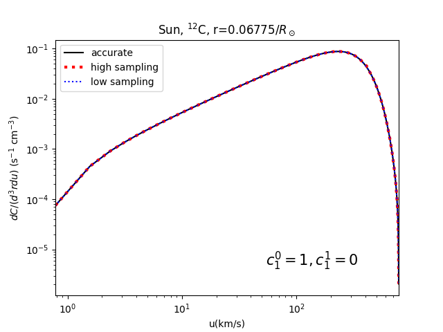
Figure 10: $\frac{dC^{T}_{ij}}{d^{3}rdu}(r,u)$ vs. $u$ at fixed $r$ = 0.5 in units of the celestial body radius for ${}^{27}Al$ and $m_{\chi}$ = 50 GeV in the Sun(left) and the Earth (right) and for SD interaction with a massless mediator.

The two plots at the bottom of Fig. 10 show a second example, corresponding to a contact interaction driven by the ${\cal O}_{1}$ operator in the Sun and in a White Dwarf. In these two plots the response functions are calculated following the same procedure of the upper plots. In particular, one can see that, as far as the Sun is concerned, a simple evaluation of the response functions with default input parameters (low sampling) is sufficient to calculate the signal accurately (the evaluations of the capture rate in the three cases, accurate, low sampling and high sampling, differ at the $10^{-4}$ level). However, in the case of the White Dwarf the low-sampling result underestimates the signal by about 30%. In this case the problem is that in a White Dwarf the escape velocity is much larger than the default value of 2000 km/s assumed in load_response_functions_capture for the maximal escape velocity, in particular implying recoil energies that extend beyond those needed for the Sun. The reason why a larger value is not assumed by default by load_response_functions_capture is to avoid a too large energy interval, for which the default sampling of 100 points would be too sparse. As shown in the plot, the high–sampling evaluation, obtained by calling wimp_capture with increase_sampling=True is sufficient to fix the problem: the capture rate in the accurate and high sampling results differ, again, at the $10^{-4}$ level.

References

- [1] I. Jeong, S. Kang, S. Scopel and G. Tomar, WimPyDD: An object–oriented Python code for the calculation of WIMP direct detection signals, Comput. Phys. Commun. 276 (2022) 108342, [2106.06207].
- [2] A. L. Fitzpatrick, W. Haxton, E. Katz, N. Lubbers and Y. Xu, The Effective Field Theory of Dark Matter Direct Detection, JCAP 1302 (2013) 004, [1203.3542].
- [3] N. Anand, A. L. Fitzpatrick and W. C. Haxton, Weakly interacting massive particle-nucleus elastic scattering response, Phys. Rev. C89 (2014) 065501, [1308.6288].
- [4] J. Silk, K. A. Olive and M. Srednicki, The Photino, the Sun and High-Energy Neutrinos, Phys. Rev. Lett. 55 (1985) 257–259.
- [5] A. Gould, Resonant Enhancements in WIMP Capture by the Earth, Astrophys. J. 321 (1987) 571.
- [6] I. Goldman and S. Nussinov, Weakly Interacting Massive Particles and Neutron Stars, Phys. Rev. D 40 (1989) 3221–3230.
- [7] D. Spolyar, K. Freese and P. Gondolo, Dark matter and the first stars: a new phase of stellar evolution, Phys. Rev. Lett. 100 (2008) 051101, [0705.0521].
- [8] P. Salati and J. Silk, A STELLAR PROBE OF DARK MATTER ANNIHILATION IN GALACTIC NUCLEI, Astrophys. J. 338 (1989) 24–31.
- [9] F. Ferrer, A. Ibarra and S. Wild, A novel approach to derive halo-independent limits on dark matter properties, JCAP 09 (2015) 052, [1506.03386].
- [10] S. Kang, A. Kar and S. Scopel, Halo-independent bounds on the non-relativistic effective theory of WIMP-nucleon scattering from direct detection and neutrino observations, PoS ICRC2023 (2023) 1371.
- [11] S. Kang, A. Kar and S. Scopel, Halo-independent bounds on Inelastic Dark Matter, JCAP 11 (2023) 077, [2308.13203].
- [12] K. Choi, I. Jeong, S. Kang, A. Kar and S. Scopel, Sensitivity of WIMP bounds on the velocity distribution in the limit of a massless mediator, JCAP 01 (2025) 007, [2408.09658].
- [13] S. Kang, I. Jeong and S. Scopel, Bracketing the direct detection exclusion plot for a WIMP of spin one half in non-relativistic effective theory, Astropart. Phys. 151 (2023) 102854, [2209.03646].
- [14] R. K. Leane and J. Smirnov, Dark matter capture in celestial objects: treatment across kinematic and interaction regimes, JCAP 12 (2023) 040, [2309.00669].
- [15] G. Belanger, A. Mjallal and A. Pukhov, Recasting direct detection limits within micrOMEGAs and implication for non-standard Dark Matter scenarios, Eur. Phys. J. C 81 (2021) 239, [2003.08621].
- [16] T. Bringmann, J. Edsjö, P. Gondolo, P. Ullio and L. Bergström, DarkSUSY 6 : An Advanced Tool to Compute Dark Matter Properties Numerically, JCAP 07 (2018) 033, [1802.03399].
- [17] T. Emken and C. Kouvaris, “DaMaSCUS: Dark Matter Simulation Code for Underground Scatterings.” Astrophysics Source Code Library, record ascl:1706.003, June, 2017.
- [18] T. Emken and C. Kouvaris, DaMaSCUS: The Impact of Underground Scatterings on Direct Detection of Light Dark Matter, JCAP 10 (2017) 031, [1706.02249].
- [19] J. Bramante, J. Kumar, G. Mohlabeng, N. Raj and N. Song, Light dark matter accumulating in planets: Nuclear scattering, Phys. Rev. D 108 (2023) 063022, [2210.01812].
- [20] N. A. Kozar, A. Caddell, L. Fraser-Leach, P. Scott and A. C. Vincent, Capt’n General: A generalized stellar dark matter capture and heat transport code, in Tools for High Energy Physics and Cosmology, 5, 2021, 2105.06810.
- [21] A. Brenner, G. Herrera, A. Ibarra, S. Kang, S. Scopel and G. Tomar, Complementarity of experiments in probing the non-relativistic effective theory of dark matter-nucleon interactions, JCAP 06 (2022) 026, [2203.04210].
- [22] D. Tucker-Smith and N. Weiner, Inelastic dark matter, Phys. Rev. D 64 (2001) 043502, [hep-ph/0101138].
- [23] P. W. Graham, R. Harnik, S. Rajendran and P. Saraswat, Exothermic Dark Matter, Phys. Rev. D 82 (2010) 063512, [1004.0937].
- [24] J. B. Dent, L. M. Krauss, J. L. Newstead and S. Sabharwal, General analysis of direct dark matter detection: From microphysics to observational signatures, Phys. Rev. D92 (2015) 063515, [1505.03117].
- [25] R. Catena, K. Fridell and M. B. Krauss, Non-relativistic Effective Interactions of Spin 1 Dark Matter, JHEP 08 (2019) 030, [1907.02910].
- [26] P. Gondolo, S. Kang, S. Scopel and G. Tomar, Effective theory of nuclear scattering for a WIMP of arbitrary spin, Phys. Rev. D 104 (2021) 063017, [2008.05120].
- [27] R. Catena and B. Schwabe, Form factors for dark matter capture by the Sun in effective theories, JCAP 1504 (2015) 042, [1501.03729].
- [28] A. Brenner, A. Ibarra and A. Rappelt, Conservative constraints on the effective theory of dark matter-nucleon interactions from IceCube: the impact of operator interference, JCAP 07 (2021) 012, [2011.02929].
- [29] E. Del Nobile, G. B. Gelmini, P. Gondolo and J.-H. Huh, Halo-independent analysis of direct detection data for light WIMPs, JCAP 1310 (2013) 026, [1304.6183].
- [30] E. Del Nobile, G. Gelmini, P. Gondolo and J.-H. Huh, Generalized Halo Independent Comparison of Direct Dark Matter Detection Data, JCAP 1310 (2013) 048, [1306.5273].
- [31] F. Kahlhoefer and S. Wild, Studying generalised dark matter interactions with extended halo-independent methods, JCAP 10 (2016) 032, [1607.04418].
- [32] M. Blennow, S. Clementz and J. Herrero-Garcia, The distribution of inelastic dark matter in the Sun, Eur. Phys. J. C 78 (2018) 386, [1802.06880].
- [33] J. F. Acevedo, J. Bramante, Q. Liu and N. Tyagi, Neutrino and gamma-ray signatures of inelastic dark matter annihilating outside neutron stars, JCAP 03 (2025) 028, [2404.10039].
- [34] A. Biswas, A. Kar, H. Kim, S. Scopel and L. Velasco-Sevilla, Improved white dwarves constraints on inelastic dark matter and left-right symmetric models, Phys. Rev. D 106 (2022) 083012, [2206.06667].
- [35] J. Bramante, A. Delgado and A. Martin, Multiscatter stellar capture of dark matter, Phys. Rev. D 96 (2017) 063002, [1703.04043].
- [36] B. Dasgupta, A. Gupta and A. Ray, Dark matter capture in celestial objects: Improved treatment of multiple scattering and updated constraints from white dwarfs, JCAP 08 (2019) 018, [1906.04204].
- [37] C. Ilie and C. Levy, Multicomponent multiscatter capture of dark matter, Phys. Rev. D 104 (2021) 083033, [2105.09765].
- [38] R. K. Leane and J. Smirnov, Dark matter capture in celestial objects: treatment across kinematic and interaction regimes, JCAP 12 (2023) 040, [2309.00669].
- [39] M. Blennow, S. Clementz and J. Herrero-Garcia, Pinning down inelastic dark matter in the Sun and in direct detection, JCAP 04 (2016) 004, [1512.03317].
- [40] R. Catena, WIMP capture and annihilation in the Earth in effective theories, JCAP 01 (2017) 059, [1609.08967].
- [41] J. F. Acevedo, R. K. Leane and L. Santos-Olmsted, Milky Way white dwarfs as sub-GeV to multi-TeV dark matter detectors, JCAP 03 (2024) 042, [2309.10843].
- [42] I. John, R. K. Leane and T. Linden, Dark Branches of Immortal Stars at the Galactic Center, 2405.12267.
- [43] S. Robles and S. A. Meighen-Berger, Extending the Dark Matter Reach of Water Cherenkov Detectors using Jupiter, 2411.04435.
- [44] C. M. Ho and R. J. Scherrer, Anapole Dark Matter, Phys. Lett. B 722 (2013) 341–346, [1211.0503].
- [45] A. L. Fitzpatrick and K. M. Zurek, Dark Moments and the DAMA-CoGeNT Puzzle, Phys. Rev. D 82 (2010) 075004, [1007.5325].
- [46] S. Kang, S. Scopel, G. Tomar, J.-H. Yoon and P. Gondolo, Anapole Dark Matter after DAMA/LIBRA-phase2, JCAP 1811 (2018) 040, [1808.04112].
- [47] IceCube collaboration, R. Abbasi et al., Searching for Dark Matter from the Sun with the IceCube Detector, PoS ICRC2021 (2022) 020.
- [48] LZ collaboration, J. Aalbers et al., Dark Matter Search Results from 4.2 Tonne-Years of Exposure of the LUX-ZEPLIN (LZ) Experiment, Phys. Rev. Lett. 135 (2025) 011802, [2410.17036].
- [49] LUX-ZEPLIN collaboration, D. S. Akerib et al., Projected WIMP sensitivity of the LUX-ZEPLIN (LZ) dark matter experiment, 1802.06039.
- [50] A. H. G. Peter, Dark matter in the solar system II: WIMP annihilation rates in the Sun, Phys. Rev. D 79 (2009) 103532, [0902.1347].
- [51] J. Kumar, J. G. Learned, S. Smith and K. Richardson, Tools for Studying Low-Mass Dark Matter at Neutrino Detectors, Phys. Rev. D 86 (2012) 073002, [1204.5120].
- [52] Z.-L. Liang and Y.-L. Wu, Direct detection and solar capture of spin-dependent dark matter, Phys. Rev. D 89 (2014) 013010, [1308.5897].
- [53] W.-L. Guo, Z.-L. Liang and Y.-L. Wu, Direct detection and solar capture of dark matter with momentum and velocity dependent elastic scattering, Nucl. Phys. B 878 (2014) 295–308, [1305.0912].
- [54] A. Serenelli, S. Basu, J. W. Ferguson and M. Asplund, New Solar Composition: The Problem With Solar Models Revisited, Astrophys. J. Lett. 705 (2009) L123–L127, [0909.2668].
- [55] R. Garani and S. Palomares-Ruiz, Evaporation of dark matter from celestial bodies, JCAP 05 (2022) 042, [2104.12757].
- [56] A. M. Dziewonski and D. L. Anderson, Preliminary reference earth model, Phys. Earth Planet. Interiors 25 (1981) 297–356.
- [57] J. Bramante, A. Buchanan, A. Goodman and E. Lodhi, Terrestrial and Martian Heat Flow Limits on Dark Matter, Phys. Rev. D 101 (2020) 043001, [1909.11683].
- [58] M. French, A. Becker, W. Lorenzen, N. Nettelmann, M. Bethkenhagen, J. Wicht et al., Ab initio simulations for material properties along the jupiter adiabat, The Astrophysical Journal Supplement Series 202 (aug, 2012) 5.
- [59] R. K. Leane and T. Linden, First Analysis of Jupiter in Gamma Rays and a New Search for Dark Matter, Phys. Rev. Lett. 131 (2023) 071001, [2104.02068].
- [60] N. F. Bell, G. Busoni, M. E. Ramirez-Quezada, S. Robles and M. Virgato, Improved treatment of dark matter capture in white dwarfs, JCAP 10 (2021) 083, [2104.14367].
- [61] I. John, R. K. Leane and T. Linden, Dark matter scattering constraints from observations of stars surrounding Sgr A*, Phys. Rev. D 109 (2024) 123041, [2311.16228].
- [62] E. Hassani, R. Pazhouhesh and H. Ebadi, The Effect of Dark Matter on Stars at the Galactic Center: The Paradox of Youth Problem, Int. J. Mod. Phys. D 29 (2020) 2050052, [2003.12451].
- [63] K. Griest and D. Seckel, Cosmic Asymmetry, Neutrinos and the Sun, Nucl. Phys. B 283 (1987) 681–705.