Expectation-propagation for Bayesian empirical likelihood inference

Abstract

Bayesian inference typically relies on specifying a parametric model that approximates the data-generating process. However, misspecified models can yield poor convergence rates and unreliable posterior calibration. Bayesian empirical likelihood offers a semi-parametric alternative by replacing the parametric likelihood with a profile empirical likelihood defined through moment constraints, thereby avoiding explicit distributional assumptions. Despite these advantages, Bayesian empirical likelihood faces substantial computational challenges, including the need to solve a constrained optimization problem for each likelihood evaluation and difficulties with non-convex posterior support, particularly in small-sample settings. This paper introduces a variational approach based on expectation-propagation to approximate the Bayesian empirical-likelihood posterior, balancing computational cost and accuracy without altering the target posterior via adjustments such as pseudo-observations. Empirically, we show that our approach can achieve a superior cost–accuracy trade-off relative to existing methods, including Hamiltonian Monte Carlo and variational Bayes. Theoretically, we show that the approximation and the Bayesian empirical-likelihood posterior are asymptotically equivalent.

1 Introduction

Consider a set of observations ${\mathcal{D}}_{n}=\{{\bm{z}}_{i}\}_{i=1}^{n}$ assumed to be drawn independently and identically distributed (i.i.d.) from a distribution $F_{0}({\bm{z}})=f({\bm{z}};{\bm{\theta}}_{0})$ indexed by ${\bm{\theta}}_{0}\in{\bm{\Theta}}\subset\mathbb{R}^{p}$. Bayesian inference provides a principled framework to learn about this parameter by updating our beliefs based on the data. Given prior information encoded in a prior distribution $p({\bm{\theta}})$, our belief about ${\bm{\theta}}$ is updated via Bayes’ rule: $p({\bm{\theta}}\mid{\mathcal{D}}_{n})\propto p({\bm{\theta}})\prod^{n}_{i=1}f({\bm{z}}_{i};{\bm{\theta}})$. The posterior distribution $p({\bm{\theta}}\mid{\mathcal{D}}_{n})$ is the central object of interest in most of Bayesian analyses. When the data distribution is correctly specified, the posterior is consistent (Doob, 1949) and asymptotically normal (Le Cam, 1953; Kleijn and van der Vaart, 2012) under a range of regularity conditions. However, the choice of an appropriate distributional family is often a difficult task. On one hand, simple data distributions impose strong assumptions which could result in invalid inference (Bissiri et al., 2016). On the other hand, elaborate distributions (e.g., mixture models) with flexible assumptions are computationally challenging to fit.

There are several non‑parametric or semi‑parametric approaches to tackle model misspecification. For example, the Dirichlet process mixtures (Ferguson, 1973; Blackwell and MacQueen, 1973; Antoniak, 1974; Lee et al., 2025) and the generalized Bayes posteriors (Grünwald, 2012; Bissiri et al., 2016) require tuning of the concentration parameter and the learning rate respectively. Such parameters are often crucial for posterior calibration, yet they can be difficult to tune. Martingale posterior (Fong et al., 2023) is another approach that requires the specification of a sequence of one‑step‑ahead predictive distributions instead of the traditional model and prior. However, a sensible predictive sequence is not always easy to obtain in practice, especially when $n$ is small.

Bayesian empirical likelihood (Lazar, 2003) is another semi-parametric approach to Bayesian inference. Rather than employing a parametric likelihood in the posterior, it replaces the likelihood with a profile empirical likelihood (Owen, 1988), which is defined as a solution to a constrained optimization problem subject to $\mathbb{E}_{{\bm{z}}\sim F_{0}}[h({\bm{z}},{\bm{\theta}})]={\bm{0}}$ for some constraint function $h$. Crucially, under this framework, there is no statistical model to be specified nor hyperparameters (e.g., concentration parameters or learning rates) to be tuned. The framework of Lazar (2003), however, is not the only way to incorporate empirical likelihood into Bayesian workflows. For instance, the exponentially tilted empirical likelihood (Schennach, 2005; Yiu et al., 2020) has been adapted to moment-misspecification settings (Chib et al., 2018). Penalised empirical likelihoods have been proposed to address degeneracy when the dimension of the constraint function $h$ is greater then the sample size $n$ (Chang et al., 2025), and profile empirical likelihood has been applied within approximate Bayesian computation (Mengersen et al., 2013). Other related Bayesian moment-based inference methods have also been introduced (Bornn et al., 2019; Florens and Simoni, 2021).

Despite its appeal, Bayesian empirical likelihood is often challenging to implement due to the profile empirical likelihood. In practice, the solution to the underlying constrained optimisation problem must be obtained numerically and may not even exist, resulting in a posterior with highly non-convex support. Consequently, efficient computation of the Bayesian empirical likelihood posterior $p_{\operatorname{EL}}$ remains an open problem. Hamiltonian Monte Carlo (HMC, Duane et al., 1987) is a common choice to approximate $p_{\operatorname{EL}}$ when the moment condition function $h$ is smooth, and it can generally provide accurate approximations (Chaudhuri et al., 2017). However, HMC may be infeasible due to computational constraints or working with non-smooth $h$. When the quantity of interest is the posterior moments, a direct estimate can be obtained without computing the problematic posterior (Vexler et al., 2014). For applications requiring fast approximation of the posterior, Yu and Bondell (2024) proposed approximating $p_{\operatorname{EL}}$ with the Gaussian minimizer of the Kullback–Leibler (KL) divergence $\operatorname*{arg\,min}_{q\in{\mathcal{Q}}}{\mathbb{E}}_{{\bm{\theta}}\sim q}[\log q({\bm{\theta}})-\log p_{\operatorname{EL}}({\bm{\theta}}\mid{\mathcal{D}}_{n})]$ within a class of Gaussian distribution ${\mathcal{Q}}$, where $p_{\operatorname{EL}}$ denotes the posterior of Bayesian empirical likelihood. Here, a mismatch between the support of $p_{\operatorname{EL}}$ and $q$ results in the KL divergence equals to infinity. To address the mismatch in support, Yu and Bondell (2024) replace $p_{\operatorname{EL}}$ with a posterior based on the adjusted empirical likelihood function (Chen et al., 2008) in the KL objective. The replacement posterior has a support matching the Gaussian distribution, and thus the KL divergence is finite. However, for a finite sample size $n$, the resultant approximate posterior is sensitive to the adjustment level in the approximate empirical likelihood, and the replacement posterior adds an extra layer of approximation to (2).

1.1 Contribution

We study expectation‑propagation (Opper and Winther, 2000; Minka, 2001), an algorithm that enjoys considerable empirical success for approximating Bayesian posteriors (Hernandez-Lobato and Hernandez-Lobato, 2016; Hasenclever et al., 2017; Hall et al., 2020). More crucially, the algorithm remains appropriate even when the supports of the approximate and the target posteriors do not match. We propose an implementation for Bayesian empirical likelihood and provide practical guidance on algorithmic stability. We formally show that $p_{\operatorname{EL}}$ is asymptotically normal and that the solution of expectation-propagation is asymptotically equivalent to $p_{\operatorname{EL}}$. Through an extensive set of experiments, we show that the algorithm achieves a better cost–accuracy trade‑off than HMC (Chaudhuri et al., 2017), without adjustments to the posterior that can impair approximation quality in small‑$n$ settings (Yu and Bondell, 2024).

This paper begins by reviewing the necessary background on Bayesian empirical likelihood and expectation-propagation in Section 2. We then present our algorithm in the context of Bayesian empirical likelihood inference in Section 3, establish its asymptotic properties in Section 4, and demonstrate its performance on a variety of modelling tasks in Section 5. We conclude in Section 6.

2 Background

We begin this section with a review of Bayesian empirical likelihood, with particular emphasis on the computational challenges of implementing it. This is followed by a review of expectation-propagation (Opper and Winther, 2000; Minka, 2001), on which our proposed method is based.

2.1 Bayesian empirical likelihood

Bayesian empirical likelihood (Lazar, 2003), building on empirical likelihood (Owen, 1988), offers a semi‑parametric alternative that avoids restrictive distributional assumptions. Rather than specifying a full data‑generating distribution, practitioners specify a moment constraint function $h:{\mathcal{Z}}\times{\bm{\Theta}}\to\mathbb{R}^{K}$ and assume that observations and ${\bm{\theta}}$ satisfy ${\mathbb{E}}_{{\bm{z}}\sim F_{0}}[h({\bm{z}},{\bm{\theta}})]={\bm{0}}$. The likelihood in the posterior is replaced by the profile empirical likelihood, $\operatorname{EL}({\bm{\theta}})$, defined as the constrained maximum

$$\operatorname{EL}({\bm{\theta}})=\max_{{\bm{w}}}\prod_{i=1}^{n}w_{i},\quad\text{subject to}\quad\sum_{i=1}^{n}w_{i}h({\bm{z}}_{i},{\bm{\theta}})={\bm{0}},\quad\sum_{i=1}^{n}w_{i}=1,$$ (1)

over discrete distributions ${\bm{w}}=\{w_{i}\}^{n}_{i=1}\in[0,1]^{n}$ on the observations $\{{\bm{z}}_{i}\}^{n}_{i=1}$. The primary aim of this work is to develop a computationally efficient method to obtain the Bayesian empirical likelihood posterior

$$p_{\operatorname{EL}}({\bm{\theta}}\mid{\mathcal{D}}_{n})\propto p({\bm{\theta}})\operatorname{EL}({\bm{\theta}}),$$ (2)

where $\operatorname{EL}({\bm{\theta}})$ depends on the observations ${\mathcal{D}}_{n}$.

One of the main bottlenecks in Bayesian empirical likelihood is the computation of (1). This constrained maximization problem can be solved by introducing a Lagrange multiplier ${\bm{\lambda}}$ with solution $w_{i}=n^{-1}(1+{\bm{\lambda}}_{\operatorname{EL}}^{\top}{\bm{h}}_{i})^{-1}$, where ${\bm{\lambda}}_{\operatorname{EL}}$ is the root of

$$\sum_{i=1}^{n}\frac{{\bm{h}}_{i}}{1+{\bm{\lambda}}_{\operatorname{EL}}^{\top}{\bm{h}}_{i}}={\bm{0}}.$$ (3)

Here, we write $\bm{h}_{i}=h({\bm{z}}_{i},{\bm{\theta}})$ for brevity. The solution ${\bm{\lambda}}_{\operatorname{EL}}$ can only exist if ${\bm{0}}$ is in the convex hull ${\mathcal{C}}_{{\bm{\theta}}}=\{\xi\in\mathbb{R}^{K}:\xi=\sum^{n}_{i=1}w_{i}{\bm{h}}_{i},\sum^{n}_{i=1}w_{i}=1,w_{i}>0\}$, i.e., the posterior (2) is supported only over ${\bm{\Theta}}_{B}=\{{\bm{\theta}}:{\bm{0}}\in{\mathcal{C}}_{{\bm{\theta}}}\}$. Owen (1988) proves that a unique solution exists if ${\bm{0}}$ is in $\mathcal{C}_{{\bm{\theta}}}$. For ${\bm{\theta}}$ where ${\bm{\lambda}}_{\operatorname{EL}}$ does not exist, it is customary to set $\operatorname{EL}({\bm{\theta}})=0$, and the resultant posterior is of the form $p_{\operatorname{EL}}({\bm{\theta}}|{\mathcal{D}}_{n})\propto p({\bm{\theta}})\prod_{i=1}^{n}w_{i}({\bm{\theta}})$ for all ${\bm{\theta}}\in{\bm{\Theta}}_{B}$.

The computation time of (2) can be prohibitive, as the root ${\bm{\lambda}}_{\operatorname{EL}}$ must be found for each evaluation of $\operatorname{EL}({\bm{\theta}})$. A more pressing difficulty is that the posterior often has highly non-convex support, particularly when $n$ is small. This is compounded by the absence of a closed-form expression for the support boundary—often the only way to determine whether a given ${\bm{\theta}}$ lies within the support is to solve for the root in (3). We outline our approach to address these difficulties in Section 3.

2.2 Expectation-Propagation

Expectation‑propagation (Opper and Winther, 2000; Minka, 2001) is a variational inference algorithm for approximating Bayesian posteriors. It requires that the target factorizes (up to a constant) and that the approximating distribution has the same form. Our posterior $p_{\operatorname{EL}}({\bm{\theta}}\mid{\mathcal{D}}_{n})\propto p({\bm{\theta}})\prod_{i=1}^{n}w_{i}({\bm{\theta}})$ satisfies this requirement. For notational convenience, let $w_{0}({\bm{\theta}})=p({\bm{\theta}})$ so that $p_{\operatorname{EL}}({\bm{\theta}}\mid{\mathcal{D}}_{n})\propto\prod_{i=0}^{n}w_{i}({\bm{\theta}})$, and refer to $q({\bm{\theta}})=\prod_{i=0}^{n}q_{i}({\bm{\theta}})$ as the approximating distribution. In EP terminology, $q_{i}$ is a site approximation, and both $w_{i}$ and $q_{i}$ are collectively known as sites.

The KL divergence is unsuitable as a variational loss when the variational support strictly contains the posterior support. A straightforward alternative is the reverse KL divergence:

$$D_{\mathrm{KL}}(p_{\operatorname{EL}}({\bm{\theta}}\mid{\mathcal{D}}_{n})\|q({\bm{\theta}}))={\mathbb{E}}_{{\bm{\theta}}\sim p_{\operatorname{EL}}({\bm{\theta}}\mid{\mathcal{D}}_{n})}[\log p_{\operatorname{EL}}({\bm{\theta}}\mid{\mathcal{D}}_{n})-\log q({\bm{\theta}})],$$ (4)

which is finite for any $q$ with larger support than $p_{\operatorname{EL}}$. However, it is typically intractable to optimize directly: common variational tools such as the log‑derivative or reparameterization tricks are not directly applicable (Mohamed et al., 2020).

Expectation‑propagation roughly minimizes (4) by iteratively updating each $q_{i}$ as follows:

1. Compute the cavity distribution $q_{-i}({\bm{\theta}})=\prod_{j\neq i}q_{j}({\bm{\theta}})$;

2. Form the tilted distribution $q_{\backslash i}({\bm{\theta}})\propto q_{-i}({\bm{\theta}})w_{i}({\bm{\theta}})$ and compute the KL-projection $\widetilde{q}_{i}=\operatorname*{arg\,min}_{q\in{\mathcal{Q}}}D_{\mathrm{KL}}(q_{\backslash i}({\bm{\theta}})\|q({\bm{\theta}}))$;

3. Update the site $q_{i}({\bm{\theta}})=\widetilde{q}_{i}({\bm{\theta}})/q_{-i}({\bm{\theta}})$.

Expectation‑propagation sidesteps direct optimization of (4). Instead, it computes the KL-projection of a ‘localized’ posterior, namely the tilted distribution $q_{\backslash i}({\bm{\theta}})$. Despite its apparent aim, the solution of expectation-propagation generally does not coincide with the minimizer of (4). Rather, under certain conditions, it behaves similarly to the Laplace approximation (Dehaene and Barthelmé, 2018); we formalize this insight in Section 4.

While the above description of expectation-propagation does not impose restriction on the approximating distribution $q$, in practice this is typically chosen to come from an exponential-family. Then, the multiplication and division of the distribution is simply the addition and substraction of its corresponding natural parameters respectively, and KL-projection can be done by matching moments of sufficient statistics between $\widetilde{q}$ and $q_{\backslash i}$. In this work, we use a Gaussian approximating distribution $q$ parameterized by its natural parameters ${\bm{\eta}}$: the linear shift ${\bm{r}}$ and precision ${\bm{Q}}$, which correspond to the mean ${\bm{\mu}}={\bm{r}}{\bm{Q}}^{-1}$ and covariance ${\bm{\Sigma}}={\bm{Q}}^{-1}$. Then, each site approximation $q_{i}$ is also Gaussian with natural parameters ${\bm{r}}_{i}$ and ${\bm{Q}}_{i}$, and the natural parameters of the global approximation are the sums: ${\bm{r}}=\sum_{i=0}^{n}{\bm{r}}_{i}$ and ${\bm{Q}}=\sum_{i=0}^{n}{\bm{Q}}_{i}$. The KL projection in Step 2 can be solved by matching the first and second moments of $\widetilde{q}$ and $q_{\backslash i}$, and this step will be discussed in details in Section 3.

3 Expectation-Propagation for Bayesian Empirical Likelihood

Our proposal to address the challenge of implementing Bayesian empirical likelihood is to approximate $p_{\operatorname{EL}}$ using expectation-propagation (Opper and Winther, 2000; Minka, 2001), which we describe in detail in this section. Throughout the rest of this paper, we refer to this algorithm as Expectation-Propagation for Bayesian Empirical Likelihood (EPEL). The majority of the discussion here is on the local KL‑projection (Step 2), which is the key step of expectation-propagation (Vehtari et al., 2020). In our setting, the KL-projection step is accomplished by matching the means and covariances of $\widetilde{q}$ and $q_{\backslash i}$, i.e., setting the linear shift $\widetilde{{\bm{r}}}_{i}$ and precision $\widetilde{{\bm{Q}}}_{i}$ of $\widetilde{q}_{i}$ to $(\mathrm{Cov}_{{\bm{\theta}}\sim q_{\backslash i}}[{\bm{\theta}}])^{-1}\mathbb{E}_{{\bm{\theta}}\sim q_{\backslash i}}[{\bm{\theta}}]$ and $(\mathrm{Cov}_{{\bm{\theta}}\sim q_{\backslash i}}[{\bm{\theta}}])^{-1}$ respectively. As the tilted distribution $q_{\backslash i}$ is known only up to a normalizing constant, we propose approximating $q_{\backslash i}$ with the Laplace approximation and importance sampling, both of which offer good algorithmic stability and a reasonable computational cost in our setting.

3.1 Approximating moments of tilted distribution

The site updates involve the moments of an intractable tilted distribution. To circumvent the intractability, we use importance sampling:

$$\widetilde{{\bm{\mu}}}_{\mathrm{IS}}=\frac{\sum^{L}_{l=1}\xi^{l}{\bm{\theta}}^{l}}{\sum^{L}_{l=1}\xi^{l}},\quad\widetilde{{\bm{\Sigma}}}_{\mathrm{IS}}=\frac{\sum^{L}_{l=1}\xi^{l}({\bm{\theta}}^{l}-\widetilde{{\bm{\mu}}}_{\mathrm{IS}})({\bm{\theta}}^{l}-\widetilde{{\bm{\mu}}}_{\mathrm{IS}})^{\top}}{\sum^{L}_{l=1}\xi^{l}},$$ (5)

where ${\bm{\theta}}^{1},\ldots,{\bm{\theta}}^{L}$ are drawn from a proposal distribution, and $\xi^{l}=\frac{q_{-i}({\bm{\theta}}^{l})\widehat{w}_{i}({\bm{\theta}}^{l})}{s({\bm{\theta}}^{l})}$ are the importance weights. The natural parameters are computed with $\widetilde{{\bm{Q}}}_{\mathrm{IS}}=\widetilde{{\bm{\Sigma}}}_{\mathrm{IS}}^{-1}$ and $\widetilde{{\bm{r}}}_{\mathrm{IS}}=\widetilde{{\bm{Q}}}_{\mathrm{IS}}\widetilde{{\bm{\mu}}}_{\mathrm{IS}}$. The precision $\widetilde{{\bm{Q}}}_{\mathrm{IS}}$ obtained this way is generally biased, but we find the bias has negligible effect on the EPEL convergence. For the proposal distribution, we suggest the Laplace approximation of $q_{\backslash i}$:

$$\widetilde{{\bm{\mu}}}_{\mathrm{LP}}=\operatorname*{arg\,max}_{{\bm{\theta}}}\log q_{\backslash i}({\bm{\theta}}),\quad\widetilde{{\bm{Q}}}_{\mathrm{LP}}=-\nabla_{{\bm{\theta}}}\nabla_{{\bm{\theta}}}\log q_{\backslash i}({\bm{\theta}})|_{{\bm{\theta}}=\widetilde{{\bm{\mu}}}_{\mathrm{LP}}}.$$ (6)

This approximation requires $\log q_{\backslash i}$ to be twice differentiable, which holds under mild conditions (Lemma 4). Operationally, we compute $\widetilde{{\bm{\mu}}}_{\mathrm{LP}}$ using a second-order Newton’s method initialized at the cavity mean. This optimizer requires the gradient $\nabla_{{\bm{\theta}}}\log q_{\backslash i}({\bm{\theta}})=\nabla_{{\bm{\theta}}}\log q_{-i}({\bm{\theta}})+\nabla_{{\bm{\theta}}}\log w_{i}({\bm{\theta}})$, where

$$\nabla_{{\bm{\theta}}}\log w_{i}({\bm{\theta}})=\frac{{\bm{h}}_{i}^{\top}{\frac{\partial\mskip 0.0mu{\bm{\lambda}}}{\partial{\bm{\theta}}}}+{\bm{\lambda}}^{\top}{\frac{\partial\mskip 0.0mu{\bm{h}}_{i}}{\partial{\bm{\theta}}}}}{1+{\bm{\lambda}}^{\top}{\bm{h}}_{i}}.$$

The Jacobian ${\frac{\partial\mskip 0.0mu{\bm{\lambda}}}{\partial{\bm{\theta}}}}$ can be derived by applying the implicit function theorem on (3). This yields the linear system

$$\left[\sum_{i=1}^{n}w_{i}^{2}{\bm{h}}_{i}{\bm{h}}_{i}^{\top}\right]{\frac{\partial\mskip 0.0mu{\bm{\lambda}}}{\partial{\bm{\theta}}}}=\sum_{i=1}^{n}w_{i}\left[n^{-1}\bm{I}-w_{i}{\bm{h}}_{i}{\bm{\lambda}}^{\top}\right]{\frac{\partial\mskip 0.0mu{\bm{h}}_{i}}{\partial{\bm{\theta}}}},$$ (7)

where $\bm{I}$ is the identity matrix. This gradient is finite if $\sum_{i=1}^{n}w_{i}^{2}{\bm{h}}_{i}{\bm{h}}_{i}^{\top}$ is invertible, i.e., $\{{\bm{h}}_{1},\ldots,{\bm{h}}_{n}\}$ spans $\mathbb{R}^{K}$. In our implementation, we use automatic differentiation (Baydin et al., 2018) to compute both the gradient and Hessian of $\log q_{\backslash i}({\bm{\theta}})$.

In practice, we often find that the first and second moments of $q_{\backslash i}$ can be well approximated using (6). Therefore, we can improve computational efficiency by avoiding importance sampling and taking (6) directly as the moment estimates for $q_{\backslash i}$. The approach is particularly suitable when the cavity $q_{-i}$ has sufficiently high precision, since the tilted distribution is then approximately Gaussian (Dehaene and Barthelmé, 2018). We therefore recommend using (6) to approximate $\widetilde{{\bm{r}}}_{i}$ and $\widetilde{{\bm{Q}}}_{i}$ when appropriate.

3.2 Implementation

With all the tools in place, we now describe EPEL. There are two variations relative to the vanilla implementation in Section 2.2. First, we use a damping factor $\alpha\in(0,1)$ to reduce the update size of the site parameters, i.e., $\Delta{\bm{\eta}}_{i}=\alpha\cdot(\widetilde{{\bm{\eta}}}_{i}-{\bm{\eta}}^{t})$ where $\widetilde{{\bm{\eta}}}_{i}$ is the natural parameter of $\widetilde{q}$ at site $i$ and ${\bm{\eta}}^{t}$ the global approximation at the $t$-th iteration, as suggested in Vehtari et al. (2020). We discovered, both empirically and also from the analysis in Theorem 7, that the updates in the early iterations tend to be noisy. Therefore, it is beneficial to restrict the update size to avoid divergence. Second, to enable algorithmic parallelization, we update the global parameters ${\bm{\eta}}$ only after all sites have been updated at least once (Dehaene and Barthelmé, 2018). The pseudocode of EPEL is presented in Algorithm 1, and further implementation details are given in Appendix A.

Initialize $t=0$, ${\bm{\eta}}^{0}=\sum_{i}{\bm{\eta}}^{0}_{i}$ for all sites $i=1,\ldots,n+1$, damping factor $\alpha<1$

repeat

    for each site $i=1,\ldots,n+1$ do

       $q_{-i}({\bm{\theta}};{\bm{\eta}}_{-i})\leftarrow$ Cavity distribution $\sum_{j\neq i}{\bm{\eta}}_{j}^{t}$

      

      $\widetilde{{\bm{\eta}}}_{i}\leftarrow$ KL-projection of $q_{\backslash i}({\bm{\theta}})\propto q_{-i}({\bm{\theta}};{\bm{\eta}}_{-i})w_{i}({\bm{\theta}})$ with either (5) or (6)

      

      $\Delta{\bm{\eta}}_{i}\leftarrow$ Site update $\alpha\cdot(\widetilde{{\bm{\eta}}}_{i}-{\bm{\eta}}^{t})$

      

      ${\bm{\eta}}^{t+1}\leftarrow{\bm{\eta}}^{t}+\sum_{i}\Delta{\bm{\eta}}_{i}$

    end for

   ${\bm{\eta}}^{t+1}_{i}\leftarrow{\bm{\eta}}^{t}_{i}+\Delta{\bm{\eta}}_{i}$

    $t\leftarrow t+1$

until $\Delta{\bm{\eta}}_{i}$ is sufficiently small for all $i=1,\ldots n+1$, and return ${\bm{\eta}}^{t+1}$

Algorithm 1 Expectation-Propagation for Bayesian Empirical Likelihood

4 Asymptotic behaviour of EPEL

In this section, we show that EPEL and $p_{\operatorname{EL}}$ are asymptotically equivalent. The results are in three parts. Firstly, we prove that one cycle of the EPEL update is asymptotically equivalent to one cycle of the Newton–Raphson algorithm (Theorem 5). Secondly, we prove the first and second moments of the EPEL posterior are asymptotically equivalent to those of the Laplace approximation of $p_{\operatorname{EL}}$ (Theorem 7). Thirdly, we establish a Bernstein–von–Mises type of result, showing that the EPEL posterior and $p_{\operatorname{EL}}$ are asymptotically equivalent and converge to the same normal distribution (Theorem 8). Unless stated otherwise, all results are stated in the limit $n\to\infty$.

For the first two results, we adapt the techniques from Dehaene and Barthelmé (2018) to the Bayesian empirical likelihood context where the support of the posterior evolves with $n$. In particular, the novelty of our work is proving the smoothness of the target log-posterior in the entire parameter space for a sufficiently large $n$ (Lemma 4). Furthermore, to the best of our knowledge, Theorem 8 is the first Bernstein–von–Mises type of result for a Bayesian semi‑parametric expectation‑propagation posterior.

Notation.

The true parameter is ${\bm{\theta}}^{\star}$, and ${\mathbb{P}}^{\star}$ denotes the probability under $F_{0}$. The negative logarithm of each target site is $\phi_{i}(\cdot)=-\log w_{i}(\cdot)$, $i=1,\ldots,n$, with $w_{0}({\bm{\theta}})$ denoting the prior $p({\bm{\theta}})$. One‑ and zero‑vectors are ${\bm{1}}_{K}$ and ${\bm{0}}_{K}$. Subscripts $i$ index sites; superscripts $t$ index iterations.

4.1 Asymptotic equivalence to Newton-Raphson updates

A cycle of EPEL is asymptotically equivalent to performing a Newton-Raphson update on the negative log-posterior $\psi(\cdot)=\sum_{i=0}^{n}\phi_{i}(\cdot)$. More concretely, with the global approximation ${\bm{r}}^{t},{\bm{Q}}^{t}$ and ${\bm{\mu}}^{t}=({\bm{Q}}^{t})^{-1}{\bm{r}}^{t}$, the $(t+1)$‑th iterate is asymptotically equivalent to

$${\bm{\mu}}^{t+1}={\bm{\mu}}^{t}-\{\psi^{(2)}({\bm{\mu}}^{t})\}^{-1}\psi^{(1)}({\bm{\mu}}^{t}),$$

with ${\bm{Q}}^{t+1}\approx\psi^{(2)}({\bm{\mu}}^{t})$ and ${\bm{r}}^{t+1}\approx{\bm{Q}}^{t+1}{\bm{\mu}}^{t}-\psi^{(1)}({\bm{\mu}}^{t})$, where it is evident that the right-hand side is the Newton-Raphson update with the current state equal to ${\bm{\mu}}^{t}$. Under the following assumptions:

1. The parameter space ${\bm{\Theta}}$ is bounded and ${\bm{\theta}}^{\star}$ is a unique interior point.

2. For countable $h({\mathcal{Z}},{\bm{\theta}})=\{h({\bm{z}},{\bm{\theta}}):{\bm{z}}\in{\mathcal{Z}}\}$: for each ${\bm{\theta}}\in{\bm{\Theta}}$, there exist $L\geq K+1$ non‑zero vectors ${\mathcal{P}}_{{\bm{\theta}}}=\{g_{1,{\bm{\theta}}},\ldots,g_{L,{\bm{\theta}}}\}$ whose convex hull contains ${\bm{0}}_{K}$ in its interior; and $\min_{a\in[L]}{\mathbb{P}}^{\star}\{h({\bm{z}},{\bm{\theta}})=g_{a,{\bm{\theta}}}\}>0$. For uncountable $h({\mathcal{Z}},{\bm{\theta}})$: for each ${\bm{\theta}}\in{\bm{\Theta}}$, there exist $L\geq K+1$ closed, connected sets ${\mathcal{G}}_{1,{\bm{\theta}}},\ldots,{\mathcal{G}}_{L,{\bm{\theta}}}$ such that any $\{g_{a}\in{\mathcal{G}}_{a,{\bm{\theta}}}\}_{a=1}^{L}$ have a convex hull with ${\bm{0}}_{K}$ in its interior and ${\bm{0}}_{K}\notin{\mathcal{G}}_{a,{\bm{\theta}}}$; the induced density of $h({\bm{z}},{\bm{\theta}})$ is strictly positive on $\bigcup_{a=1}^{L}{\mathcal{G}}_{a,{\bm{\theta}}}$; and $\min_{a\in[L]}{\mathbb{P}}^{\star}\{h({\bm{z}},{\bm{\theta}})\in{\mathcal{G}}_{a,{\bm{\theta}}}\}>0$.

3. The first, second, and third derivatives of $h({\bm{z}},{\bm{\theta}})$ with respect to ${\bm{\theta}}$ are continuously differentiable on ${\bm{\Theta}}$ for all ${\bm{z}}\in{\mathcal{Z}}$.

4. The prior $p({\bm{\theta}})$ is positive on a neighbourhood of ${\bm{\theta}}^{\star}$. Moreover, there exists $M_{p}>0$ such that, for all $(a,b,c,d)\in\{1,\ldots,p\}^{4}$,

   $$\left|{\frac{\partial^{\mskip 1.0mu4}\mskip 0.0mu\log p({\bm{\theta}})}{\partial\theta_{a}\mskip 2.0mu plus 1.0mu minus 1.0mu\partial\theta_{b}\mskip 2.0mu plus 1.0mu minus 1.0mu\partial\theta_{c}\mskip 2.0mu plus 1.0mu minus 1.0mu\partial\theta_{d}}}\right|\leq M_{p}\quad\text{for all }{\bm{\theta}}\in{\bm{\Theta}}.$$

Assumption (I) is a standard condition for Bernstein-von-Mises type of results in empirical likelihood and mirrors many of the previous works, e.g., (Chernozhukov and Hong, 2003; Chib et al., 2018; Zhao et al., 2020; Yiu et al., 2020). Assumption (II) is a restriction on $h$. Intuitively, it requires that, for each ${\bm{\theta}}\in{\bm{\Theta}}$, there is a non-zero probability of ${\mathcal{C}}_{{\bm{\theta}}}$ containing ${\bm{0}}_{K}$ in its interior; more details in (Appendix B). This assumption also implies $\operatorname{span}({\mathcal{P}}_{{\bm{\theta}}})=\mathbb{R}^{K}$ and $\operatorname{span}(\{g_{a}\in{\mathcal{G}}_{a,{\bm{\theta}}}\}_{a=1}^{L})=\mathbb{R}^{K}$, since a ${\mathcal{P}}_{{\bm{\theta}}}$ that spans a $K-1$ or lower dimension subspace of $\mathbb{R}^{K}$ can never contain ${\bm{0}}_{K}$ in its interior. Assumptions (III) and (IV) imply that $h({\bm{z}},{\bm{\theta}})$ is differentiable with respect to ${\bm{\theta}}$ up to the fourth-order in the domain ${\bm{\Theta}}$ for all ${\bm{z}}\in{\mathcal{Z}}$. Fourth-order differentiability is needed for analysing the behaviour of EPEL, as we need the quadratic expansion of the Hessian of $\phi^{(2)}({\bm{\theta}})$. The above assumptions allow us to establish a smoothness condition for the empirical likelihood function in the entire parameter space ${\bm{\Theta}}$:

Lemma 1.

Assume (I) to (III) hold. Then, for a sufficiently large $n$,

$$\left|{\frac{\partial^{\mskip 1.0mu4}\mskip 0.0mu\phi_{i}({\bm{\theta}};{\mathcal{D}}_{n})}{\partial\theta_{a}\mskip 2.0mu plus 1.0mu minus 1.0mu\partial\theta_{b}\mskip 2.0mu plus 1.0mu minus 1.0mu\partial\theta_{c}\mskip 2.0mu plus 1.0mu minus 1.0mu\partial\theta_{d}}}\right|<\infty,\quad\emph{for all}\ (a,b,c,d)\in\{1,\dots,p\}^{4},\ i=1,\ldots,n,\ {\bm{\theta}}\in{\bm{\Theta}}.$$

The details are in Appendix C.2.

We state the following result that establishes the asymptotic equivalence of one EPEL cycle to one Newton-Raphson cycle:

Theorem 1.

Assume (I) to (IV) hold. Consider the EPEL Gaussian approximation at iteration $t$, $\{{\bm{r}}^{t}_{i}\}_{i=0}^{n}$ and $\{{\bm{Q}}_{i}^{t}\}_{i=0}^{n}$ for the linear-shift and precision of the site approximations. The global approximation mean ${\bm{\mu}}^{t}=\{\sum_{i}{\bm{Q}}_{i}^{t}\}^{-1}\sum_{i}{\bm{r}}^{t}_{i}$ is a fixed vector, and the global precision and linear-shift are ${\bm{Q}}^{t}=\sum_{i=0}^{n}{\bm{Q}}_{i}^{t}$ and ${\bm{r}}^{t}=\sum_{i=0}^{n}{\bm{r}}_{i}^{t}$ respectively. Moreover, assume that (i) $\min_{i}\min\operatorname{eigen}(\sum_{j\neq i}{\bm{Q}}_{j}^{t})=pn+O_{p}(1)$ with some positive constant $p$; (ii) the means of the tilted distributions are not too far apart, i.e., $\sum_{i}\lVert{\bm{r}}^{t}_{i}-{\bm{Q}}_{i}^{t}{\bm{\mu}}^{t}+\phi_{i}^{(1)}({\bm{\mu}}^{t})\rVert=O_{p}(n)$. Then, the new global linear shift and new global precision after one EP cycle has the asymptotic behaviour:

$$\left\lVert{\bm{r}}^{t+1}+\psi^{(1)}({\bm{\mu}}^{t})-{\bm{Q}}^{t+1}{\bm{\mu}}^{t}\right\rVert=O_{p}(1)$$

and

$$\left\lVert{\bm{Q}}^{t+1}-\psi^{(2)}({\bm{\mu}}^{t})\right\rVert=O_{p}(1)$$

where $\psi(\cdot)=\sum_{i=0}^{n}\phi_{i}(\cdot)$.

Sketch of proof.

We first show the update of each individual site ${\bm{r}}_{i}^{t}$ and ${\bm{Q}}_{i}^{t}$ is equivalent to the first and second derivatives of $\phi_{i}$ evaluated at ${\bm{\theta}}={\bm{\mu}}^{t}$ (Theorem 4). The key step of Theorem 4 is the application of Brascamp-Lieb inequality to upper-bound the covariance of the tilted distribution, then Taylor expand the terms in the upper-bound. Our stated result in this theorem follows by an application of the triangle inequality and Theorem 4. Details are provided in Appendix C.3. ∎

Remarks.

This theorem shows that, for a sufficiently large $n$, EPEL behaves like Newton-Raphson if EPEL is initialized with a sufficiently large precision, and the cavity and global mean are not too far apart. This connection is important to establish the convergence of EPEL.

4.2 Convergence of EPEL

Let $\widehat{{\bm{\theta}}}=\operatorname*{arg\,min}_{{\bm{\theta}}}\psi({\bm{\theta}})$ be the maximum-a-posteriori solution. We now prove that ${\bm{Q}}^{t}$ and ${\bm{r}}^{t}$ are asymptotically equivalent to that of the Laplace approximation of $p_{\operatorname{EL}}$, with precision $\psi^{(2)}(\widehat{{\bm{\theta}}})$ and linear shift $\psi^{(2)}(\widehat{{\bm{\theta}}})\widehat{{\bm{\theta}}}-\psi^{(1)}(\widehat{{\bm{\theta}}})$. We also prove that EPEL converges in two iterations.

Theorem 2.

Assume (I) to (IV) hold. Consider the EPEL Gaussian initializations $\{{\bm{r}}_{i}^{0}\}_{i=0}^{n}$ and $\{{\bm{Q}}_{i}^{0}\}_{i=0}^{n}$ that satisfy

$$n\max_{i}\lVert{\bm{Q}}_{i}^{0}\widehat{{\bm{\theta}}}-\phi_{i}^{(1)}(\widehat{{\bm{\theta}}})-{\bm{r}}_{i}^{0}\rVert=\Delta_{{\bm{r}}}^{0}$$

and

$$n\max_{i}\lVert\phi_{i}^{(2)}(\widehat{{\bm{\theta}}})-{\bm{Q}}_{i}^{0}\rVert=\Delta_{{\bm{\beta}}}^{0},$$

where $\Delta_{{\bm{r}}}^{0}=\sqrt{n}$ and $\Delta_{{\bm{\beta}}}^{0}=\tfrac{1}{2}\lVert\psi^{(2)}(\widehat{{\bm{\theta}}})\rVert$. Then, for every $t=1,2,\ldots$, there exists a $\Delta_{{\bm{r}}}^{t}$ and $\Delta_{{\bm{\beta}}}^{t}$ such that

$$\lVert{\bm{Q}}_{i}^{t}\widehat{{\bm{\theta}}}-\phi_{i}^{(1)}(\widehat{{\bm{\theta}}})-{\bm{r}}_{i}^{t}\rVert\leq n^{-1}\Delta_{{\bm{r}}}^{t}$$

and

$$\lVert\phi_{i}^{(2)}(\widehat{{\bm{\theta}}})-{\bm{Q}}_{i}^{t}\rVert\leq n^{-1}\Delta_{{\bm{\beta}}}^{t},$$

where $\{{\bm{r}}_{i}^{t}\}_{i=0}^{n}$ and $\{{\bm{Q}}_{i}^{t}\}_{i=0}^{n}$ denote the EP approximation parameters after the $t$-th cycle. Moreover, if $n^{-1}\psi^{(2)}(\widehat{{\bm{\theta}}})$ converges in probability to a constant positive definite matrix ${\bm{V}}_{{\bm{\theta}}^{\star}}$ with finite eigenvalues, $\sum_{i=0}^{n}\lVert\phi_{i}^{(1)}(\widehat{{\bm{\theta}}})\rVert=O_{p}(n)$, and $\sum_{i=0}^{n}\lVert\phi_{i}^{(2)}(\widehat{{\bm{\theta}}})\rVert=O_{p}(n)$, then

$$\Delta_{{\bm{r}}}^{t}=O_{p}(1)\quad\emph{and}\quad\Delta_{{\bm{\beta}}}^{t}=O_{p}(1)\quad\emph{for all}\quad t=2,3\ldots.$$

Sketch of proof.

We start from the bounds in Theorem 4 and replace ${\bm{\mu}}^{t}$ with $\widehat{{\bm{\theta}}}$ via Taylor expansions and algebra. This yields recursive bounds in terms of $\Delta_{{\bm{r}}}^{t}$ and $\Delta_{{\bm{\beta}}}^{t}$. We substitute the initial $\Delta_{{\bm{r}}}^{0}$ and $\Delta_{{\bm{\beta}}}^{0}$ to obtain the stated rates. ∎

Remarks.

By the triangle inequality, $\lVert{\bm{Q}}^{t}\widehat{{\bm{\theta}}}-\psi^{(1)}(\widehat{{\bm{\theta}}})-{\bm{r}}^{t}\rVert\leq\Delta_{{\bm{r}}}^{t}$ and $\lVert\psi^{(2)}(\widehat{{\bm{\theta}}})-{\bm{Q}}^{t}\rVert\leq\Delta_{{\bm{\beta}}}^{t}$. Notably, the first iteration has $\Delta_{{\bm{\beta}}}^{1}=O_{p}(\sqrt{n})$ and $\Delta_{{\bm{r}}}^{1}=O_{p}(1)$. Empirically, we also observe a spike in ${\bm{Q}}^{1}$ in the first iteration, followed by gradual convergence. The first and second moments of EPEL are asymptotically equivalent to that of the Laplace approximation of $p_{\operatorname{EL}}$ after at least two iterations under the required assumptions. Details are provided in Appendix C.4.

4.3 EPEL Bernstein-von-Mises Theorem

Finally, we establish a Bernstein–von–Mises result for EPEL under the stability conditions from Theorem 7 and iterations of at least two cycles. The Bayesian empirical‑likelihood posterior $p_{\operatorname{EL}}$ is asymptotically normal and equivalent to the EPEL solution. For this result, we require the following additional assumptions, which are common in the Bayesian semi-parametric setting:

1. We assume ${\bm{S}}^{\star}={\mathbb{E}}\left[h({\bm{z}},{\bm{\theta}}^{\star})h({\bm{z}},{\bm{\theta}}^{\star})^{\top}\right]$ is positive definite with bounded entries.

2. For any $a>0$, there exists $\nu_{EL}>0$ such that as $n\rightarrow\infty$, we have

   $$\lim_{n\rightarrow\infty}{\mathbb{P}}^{\star}\left(\sup_{\lVert{\bm{\theta}}-{\bm{\theta}}^{\star}\rVert\geq a}n^{-1}\left\{\log\operatorname{EL}_{n}({\bm{\theta}})-\log\operatorname{EL}_{n}({\bm{\theta}}^{\star})\right\}\leq-\nu_{\operatorname{EL}}\right)=1$$

3. The quantities $\lVert\partial h({\bm{z}},{\bm{\theta}}^{\star})/\partial{\bm{\theta}}\rVert$, $\lVert\partial^{2}h({\bm{z}},{\bm{\theta}})/\partial{\bm{\theta}}\partial{\bm{\theta}}^{\top}\rVert$, $\lVert h({\bm{z}},{\bm{\theta}})\rVert^{3}$ are bounded by some integrable function $\widetilde{G}({\bm{z}})$ in a neighbourhood of ${\bm{\theta}}^{\star}$.

4. We assume ${\bm{D}}={\mathbb{E}}\{\partial h({\bm{z}},{\bm{\theta}})/\partial{\bm{\theta}}\}$ is full rank, where the expectation is taken with respect to the true distribution of ${\bm{z}}$.

Theorem 3.

Assume conditions (I) to (VIII) hold. Consider the EPEL Gaussian posterior parameterized by the linear-shift ${\bm{r}}=\sum_{i=1}^{n}{\bm{r}}_{i}$, precision ${\bm{Q}}=\sum_{i=1}^{n}{\bm{Q}}_{i}$ that are obtained after at least two EP cycles with initializations $\{{\bm{r}}_{i}^{0}\}_{i=0}^{n}$ and $\{{\bm{Q}}_{i}^{0}\}_{i=0}^{n}$ that satisfy

$$n\max_{i}\lVert{\bm{Q}}_{i}^{0}\widehat{{\bm{\theta}}}-\phi_{i}^{(1)}(\widehat{{\bm{\theta}}})-{\bm{r}}_{i}^{0}\rVert=\Delta_{{\bm{r}}}^{0}$$

and

$$n\max_{i}\lVert\phi_{i}^{(2)}(\widehat{{\bm{\theta}}})-{\bm{Q}}_{i}^{0}\rVert=\Delta_{{\bm{\beta}}}^{0},$$

where $\Delta_{{\bm{r}}}^{0}=\sqrt{n}$ and $\Delta_{{\bm{\beta}}}^{0}=\tfrac{1}{2}\lVert\psi^{(2)}(\widehat{{\bm{\theta}}})\rVert$. Then, we have

$$d_{\mathrm{TV}}(\mathcal{N}({\bm{r}},{\bm{Q}}),p_{\operatorname{EL}}({\bm{\theta}}\mid{\mathcal{D}}_{n}))=o_{p}(1).$$

Sketch of proof.

First, we show that the asymptotic behaviour of $\psi$ and $\phi_{i}$ satisfy the rates required in Theorem 7. We first show that the total variation distance between the EPEL solution and the Laplace approximation is $O_{p}(n^{-1/2})$. We then show the total variation distance between the posterior $p_{\operatorname{EL}}$ and the Laplace approximation is $o_{p}(1)$ (Lemma 7). Applying triangle inequality yields the claim. Details are provided in Appendix C.5. ∎

5 Experiments

In this section, we examine the cost–accuracy trade-off across different methods to compute the posterior of Bayesian empirical likelihood. The methods under consideration are: HMC (Chaudhuri et al., 2017), variational Bayes (Yu and Bondell, 2024) with a full-covariance Gaussian variational distribution, and the Metropolis–Hastings algorithm with a random-walk proposal. We compare the methods across a range of settings: linear regression, logistic regression, quantile regression, and generalized estimating equations. Of particular note is quantile regression, whose moment constraint function $h$ is non-differentiable.

We tracked the posterior approximation for each method over many iterations. For HMC and MCMC, this was the empirical distribution of the cumulative samples. For variational Bayes and EPEL, it was the current variational approximation to $p_{\operatorname{EL}}({\bm{\theta}}\mid{\mathcal{D}}_{n})$. The posterior approximations were compared against a ‘gold standard’ to assess their quality. This gold standard was an empirical distribution formed by either $2\times 10^{6}$ draws from an HMC sampler for examples with a differentiable $h$, or otherwise $10^{7}$ draws from the Metropolis–Hastings algorithm. The exact implementation and hyperparameters of these algorithms are given in Appendix D.

To assess the difference between the gold standard and each posterior approximation, we drew 1000 samples from each and computed the optimal non-bipartite pairings (NBPs; Derigs, 1988). The NBP computation was done on the pooled 2000 samples (1000 from each of the gold standard and the assessed method). We then counted the cross-match NBPs, which are pairs with exactly one sample from the gold standard and one sample from the assessed method. A larger number of cross-match NBPs indicates that the two distributions are more similar. We used 474 pairs as a cut-off to determine whether an approximate posterior had achieved sufficient accuracy. This threshold corresponds to the 0.05 quantile of the NBP statistic’s exact null distribution (based on 1000 pseudo-samples), i.e., $\Pr(\mathrm{NBP}\geq 474)\geq 0.5$, under the null hypothesis that the approximation is identical to the gold-standard posterior. An NBP reading greater than 474 would fail to reject the null hypothesis and suggests that the two distributions are statistically indistinguishable. The NBPs were computed with the nbpMatching R package (Beck et al., 2024).

We assigned a ${\mathcal{N}}(0,10^{2})$ prior on each element of ${\bm{\theta}}$. The EPEL and variational Bayes are initialized with the Laplace approximation of $p_{\operatorname{EL}}$. This initial approximation is also included as a baseline in our comparisons. The sites of EPEL ${\bm{\eta}}^{0}_{i}$ are initialized as ${\bm{\eta}}^{0}_{i}={\bm{\eta}}^{0}/(n+1)$ where ${\bm{\eta}}^{0}$ is the natural parameter corresponding to the Laplace approximation of $p_{\operatorname{EL}}$. For the MCMC methods (HMC and Metropolis–Hastings), we used a burn-in period before collecting samples. All results are averaged over 50 independent runs.

We implemented all methods with JAX (Bradbury et al., 2018), a Python package which facilitates automatic differentiation and obviates the need for manual derivations of derivatives for gradient-based methods. The code is compiled, but all wall-clock time measurements exclude compilation time. We ran our experiments in containers to ensure reproducibility. Each container was assigned with two virtual cores and sufficient memory. The workload was run on AMD EPYC 9474F 3.6 GHz processors. Code is available at https://github.com/weiyaw/epel.

5.1 Linear regression

We start with a relatively simple linear regression problem to contrast performance in large- and small-$n$ settings. The data were generated from $y_{i}={\bm{x}}_{i}^{\top}{\bm{\theta}}_{0}+\epsilon_{i},i=1,\ldots,100$, where ${\bm{x}}_{i}=(1,x_{i1},\ldots,x_{i;(p-1)})^{\top}$ and $\epsilon_{i}\sim\mathcal{N}(0,1)$. The covariates were drawn from the standard normal distribution, $x_{ij}\sim\mathcal{N}(0,1)$ for all $j=1,\ldots,p-1$. We consider both $p=2$, ${\bm{\theta}}_{0}=(0.5,1)^{\top}$ and $p=10$, ${\bm{\theta}}_{0}=(0.5,1,0.5,-1,0.5,0,\ldots,0)^{\top}$ examples. The vector of regression coefficients, ${\bm{\theta}}$, is our parameter of interest. In Bayesian empirical likelihood, we avoid specifying the distribution of $\epsilon$ as in the usual parametric approach. Rather, it is common to assume the data satisfy a weaker orthogonality constraint, ${\mathbb{E}}_{(y,{\bm{x}})\sim F_{0}}[{\bm{x}}(y-{\bm{x}}^{\top}{\bm{\theta}})]={\bm{0}}_{p}$. The constraint function is therefore $h({\bm{z}},{\bm{\theta}})={\bm{x}}(y-{\bm{x}}^{\top}{\bm{\theta}})$, where ${\bm{z}}=(y,{\bm{x}})$.

The results are presented in Figure 1. In the $p=2$ example (Figure 1(a)), where $n$ is much larger than $p$, we observe that EPEL, the Laplace approximation, and variational Bayes are all similar to the gold standard, as predicted by Theorem 8 and Yu and Bondell (2024). The same cannot be said in the larger $p$ setting, where $n$ is small relative to $p$. For variational Bayes, the multi-layered approximation framework manifests in the output: the method struggles to attain a sufficiently accurate posterior approximation. Similarly, the Laplace approximation is barely close to the posterior. However, EPEL can still attain sufficient accuracy in this setup. For sampling-based HMC and Metropolis–Hastings, they can generally produce a good approximation to the posterior when given enough compute budget (e.g., for HMC, 10 and 50 seconds in $p=2$ and $p=10$, respectively). EPEL is much more computationally efficient and can achieve the same accuracy as HMC almost instantaneously here.

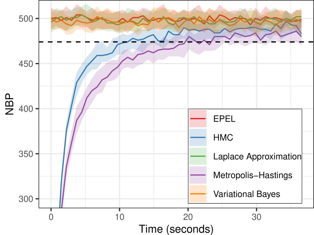
(a) $p=2$

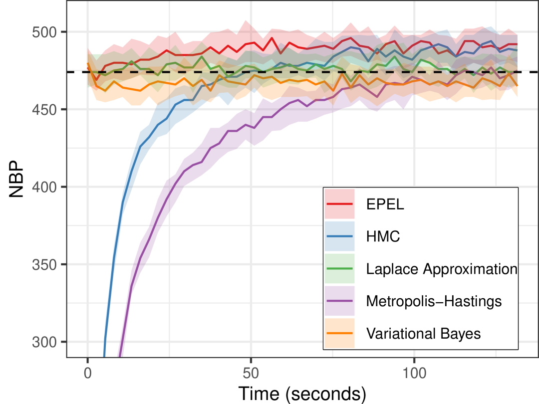
(b) $p=10$

Figure 1: Linear regression for $p=2$ and $p=10$. Coloured curves are median NBP with respect to the gold standard across 50 repetitions. Shaded areas denote the 0.25–0.75 quantiles. The dotted line at 474 denotes the threshold. On the left, the algorithms operate in the large-$n$ regime, and the Laplace approximation, EPEL and variational Bayes are indistinguishable from the gold standard. On the right, EPEL achieves a better cost–accuracy trade-off.

5.2 Quantile regression

In this example, we demonstrate an application with a non-smooth $h$. We perform quantile regression to estimate a function ${\bm{x}}\mapsto{\bm{x}}^{\top}{\bm{\theta}}$ such that $\text{Pr}(y\leq{\bm{x}}^{\top}{\bm{\theta}}\mid{\bm{x}})=\tau$ for some quantile $\tau\in[0,1]$. Here, we set $\tau=0.7$. We use the dataset from the previous linear regression example with ${\bm{\theta}}_{0}=(0.5,1)^{\top}$. Quantile regression with Bayesian empirical likelihood has previously been studied in Yang and He (2012). In their work, they suggest the constraint function $h({\bm{x}},y,{\bm{\theta}})=\rho_{\tau}(y-{\bm{x}}^{\top}{\bm{\theta}}){\bm{x}}$, where

$$\rho_{\tau}(u)=\begin{cases}1-\tau,&u<0,\\ 0,&u=0,\\ -\tau,&u>0,\end{cases}$$

is the quantile score function. This form of $h$ has zero value for $\nabla_{{\bm{\theta}}}h$ almost everywhere, and is problematic for gradient-based methods, e.g., HMC and variational Bayes. For methods that require a well-behaved $\nabla_{{\bm{\theta}}}h$, we replace $\rho_{\tau}$ with a smooth approximation, $\widetilde{\rho}_{\tau}(u)=\operatorname{expit}(-u/\epsilon_{\rho})-\tau$, with a sufficiently small $\epsilon_{\rho}$. We use $\epsilon_{\rho}=0.1$ in our experiment.

A well-behaved $\nabla_{{\bm{\theta}}}h$ is not strictly necessary for EPEL if $q_{\backslash i}$ is approximated with importance sampling. In practice, we prefer the Laplace-based computation of $q_{\backslash i}$, as we observed substantial gains in computation time with negligible impact on accuracy from approximating $\rho_{\tau}$.

From Figure 2, we observe that all methods, apart from the Laplace approximation, produced good approximations. Variational Bayes was the quickest (almost instantaneously) to achieve sufficient quality, followed by EPEL (9 seconds), HMC (14 seconds), and Metropolis–Hastings (16 seconds). The smooth approximation to $\rho_{\tau}$ also had negligible impact on approximation quality within our computation-time constraints, as the outputs of these methods were similar in quality.

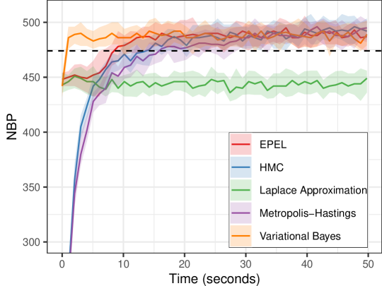
Figure 2: Quantile regression. Coloured curves are median NBP with respect to the gold standard across 50 repetitions. Shaded areas denote the 0.25–0.75 quantiles. The dotted line at 474 denotes the threshold. Variational Bayes achieves the best cost–accuracy trade-off, followed by EPEL and the sampling-based methods. The Laplace approximation never attains sufficient accuracy.

5.3 Logistic regression with the Kyphosis data

We demonstrate the methods on the Kyphosis dataset (Chambers and Hastie, 1992) with a logistic regression model. The dataset contains the outcomes of 81 children after corrective spinal surgery. The response variable is binary (absence or presence of kyphosis after surgery) and the covariates are the age of the child, the number of vertebrae involved in the surgery, and the number of the topmost vertebra operated on. We fit a logistic regression model

$$\operatorname{logit}\left(\frac{y_{i}}{1-y_{i}}\right)={\bm{x}}^{\top}_{i}{\bm{\theta}},\quad i=1,\ldots,81,$$

with covariates ${\bm{x}}_{i}=(1,x_{i1},x_{i2},x_{i3})^{\top}$, a binary response $y_{i}$, and ${\bm{\theta}}=(\theta_{0},\ldots,\theta_{3})^{\top}$. The dataset was obtained from the rpart R package. The covariates were standardized before model fitting. We again have an orthogonality constraint $h(y,{\bm{x}},{\bm{\theta}})={\bm{x}}(y-\operatorname{expit}({\bm{x}}^{\top}{\bm{\theta}}))$.

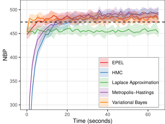
Figure 3: Logistic regression on the Kyphosis dataset. Coloured curves are median NBP with respect to the gold standard across 50 repetitions. Shaded areas denote the 0.25–0.75 quantiles. The dotted line at 474 denotes the threshold. Variational Bayes and EPEL have almost the same cost–accuracy trade-off. The sampling-based methods eventually approximate the posterior better than the variational methods. The Laplace approximation never attains sufficient accuracy.

The result of this real-world example is similar to that of the quantile regression example. Both EPEL and variational Bayes attained good approximations relatively quickly (5 seconds for the former; almost instantaneously for the latter) compared to Metropolis–Hastings (14 seconds) and HMC (20 seconds). Both Metropolis–Hastings and HMC also overtook EPEL and variational Bayes roughly after 30 seconds. The Laplace approximation performed poorly in this example.

5.4 Generalized estimating equations

We conclude with an example using generalized estimating equations, a classical technique for estimating regression coefficients in longitudinal data analysis. In this example, we adopt the over-identification case, i.e., the number of estimating equations is greater than $p$, from Chang et al. (2018). Our data were generated from a repeated-measures model ${\bm{y}}_{i}={\bm{x}}^{\top}_{i}{\bm{\theta}}_{0}+{\bm{\epsilon}}_{i},i=1,\ldots,50$, where ${\bm{\theta}}_{0}=(3,1.5,0,0,2)^{\top}$, ${\bm{y}}_{i}=(y_{i1},y_{i2})^{\top}$, ${\bm{x}}_{i}=(x_{ijk})^{p,2}_{j,k=1}\in\mathbb{R}^{p\times 2}$, and ${\bm{\epsilon}}_{i}=(\epsilon_{i1},\epsilon_{i2})^{\top}$. The $(x_{ij1},\ldots,x_{ijp})^{\top}$ are generated from $\mathcal{N}({\bm{0}},{\bm{\Sigma}})$ with ${\bm{\Sigma}}=(0.5^{\lvert k-l\rvert})^{p,p}_{k,l=1}\in\mathbb{R}^{p\times p}$. The ${\bm{\epsilon}}_{i}$ are generated from a bivariate Gaussian distribution with zero mean and unit-marginal compound-symmetry covariance matrix with off-diagonal terms set to $0.7$. We use the quadratic inference function introduced in Qu et al. (2000) to construct the constraint function

$$h({\bm{y}},{\bm{x}},{\bm{\theta}})=\begin{bmatrix}{\bm{x}}\bm{M}_{1}({\bm{y}}-{\bm{x}}^{\top}{\bm{\theta}})\\ {\bm{x}}\bm{M}_{2}({\bm{y}}-{\bm{x}}^{\top}{\bm{\theta}}),\end{bmatrix}$$

where $\bm{M}_{1}$ is a two-dimensional identity matrix, and $\bm{M}_{2}$ a unit-marginal compound-symmetry covariance matrix with off-diagonal terms set to $0.7$.

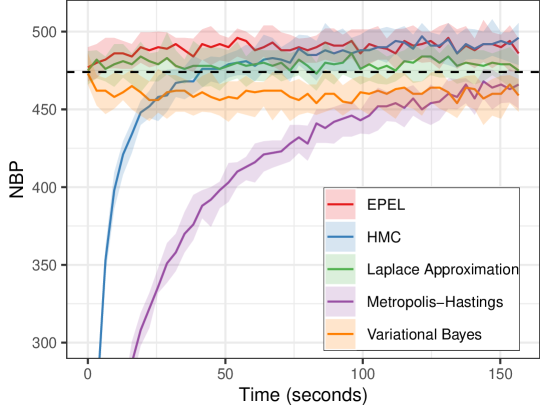
Figure 4: Generalized estimating equations. Coloured curves are median NBP with respect to the gold standard across 50 repetitions. Shaded areas denote the 0.25–0.75 quantiles. The dotted line at 474 denotes the threshold. EPEL has the best cost–accuracy trade-off, while variational Bayes never attains sufficient accuracy due to pseudo-observations in the posterior.

In this example, EPEL and HMC both achieved the highest approximation quality, with EPEL taking roughly half the time (50 seconds) compared to HMC (100 seconds). The Laplace approximation also attained sufficient approximation quality, albeit worse than EPEL and HMC. Variational Bayes did not achieve sufficient approximation accuracy. Metropolis–Hastings also did not achieve a good approximation, although we expect it to improve with more computation time.

6 Discussion

Computing the posterior of Bayesian empirical likelihood is a challenging and costly endeavor. To address this, we propose EPEL, a computationally efficient alternative to existing methods. For sufficiently large datasets and under standard regularity conditions, we show that EPEL and the exact posterior of Bayesian empirical likelihood are asymptotically equivalent. Through extensive experiments, we also demonstrate that EPEL generally achieves a better cost–accuracy trade-off than HMC, while avoiding the problematic multi-layered approximations in variational Bayes empirical likelihood when $n$ is small relative to $p$. Furthermore, EPEL does not require a differentiable constraint function and is useful for models for which a smooth approximation of the constraint is unavailable.

Like all methods, EPEL has limitations. First, our theoretical justification covers only the case in which the approximate posterior is Gaussian. Such Gaussian approximations may be inappropriate in rare circumstances where the posterior is a product of multiple empirical likelihoods; see, e.g., Chaudhuri and Ghosh (2011). Second, the algorithm may occasionally fail due to non-convergence of the inner-loop optimization used for importance sampling. Third, our proposed approximate posterior is justified only when $p<n$. We leave extensions to high-dimensional Bayesian empirical likelihood inference (Chang et al., 2025) for future work.

Appendix A Further numerical considerations for EPEL

Practical consideration for importance sampler.

We monitor the effective sample size (Gelman et al., 2013, Eq. 11.8) to determine the quality of the approximations. For numerical stability when computing $\widetilde{{\bm{\Sigma}}}_{\mathrm{IS}}$, we perform QR decomposition on the weighted scatter matrix ${\bm{S}}={\bm{Q}}{\bm{R}}$, where each row of ${\bm{S}}$ is $\sqrt{\xi^{l}}({\bm{\theta}}^{l}-\widetilde{{\bm{\mu}}}_{\mathrm{IS}})^{\top}$. Then, $\widetilde{{\bm{\Sigma}}}_{\mathrm{IS}}=(\sum^{L}_{l=1}\xi^{l})^{-1}{\bm{R}}^{\top}{\bm{R}}$, and $\widetilde{{\bm{Q}}}_{\mathrm{IS}}$ can be obtained directly from ${\bm{R}}$.

Reducing the number of sites.

To increase computational efficiency, the individual terms in $\operatorname{EL}({\bm{\theta}})$ can be pooled to reduce the number of sites. That is, the global approximation is $q({\bm{\theta}})=\prod_{j=1}^{D}q_{j}({\bm{\theta}})$, where $D<n+1$ is the number of sites and each of these $q_{j}({\bm{\theta}})$ will correspond to multiple $w_{i}$.

‘Warm-up’ cycles using Laplace approximate updates.

The expectation-propagation algorithm is widely known to be numerical unstable, especially with poor initializations. To improve numerical stability, we introduce warm-up cycles in the EPEL procedure with the moments of the Laplace approximate posterior as the updates for $\widetilde{{\bm{\eta}}}_{i}$. Once $\|\Delta{\bm{\eta}}_{i}\|$ is small, we switch over to importance sampling to ensure we are indeed approximating the moments of the tilted distributions.

Positive-definiteness of the precision of Laplace’s approximation.

Laplace’s approximation requires a numerical optimizer to compute the mode of the target distribution. Due to machine precision errors, the optimizer may not converge sufficiently close to the mode, and the Hessian at the optimizer solution can be substantially different from that at the true mode. The negative Hessian may not even be positive-definiteness, yielding an ill-defined approximation. When this occurs when approximating $q_{\backslash i}$, we use importance sampling as a fallback, using either the cavity $q_{-i}$ or the current global approximation $q^{t}$ as the proposal; the latter is guaranteed to be a proper by construction.

Positive‑definiteness of the global precision.

Since ${\bm{Q}}^{t}$ is updated with addition and subtraction, the new update ${\bm{Q}}^{t+1}$ may not be positive‑definite. We enforce positive‑definiteness by starting from a positive‑definite ${\bm{Q}}^{0}$ and dynamically decreasing the damping factor if the proposed update $\sum_{i}\Delta{\bm{\eta}}_{i}$ would render ${\bm{Q}}^{t+1}$ improper. Nonetheless, this procedure does not guarantee positive‑definiteness of each site precision ${\bm{Q}}_{i}$, which is acceptable as the site approximations are intermediate quantities (Vehtari et al., 2020).

Appendix B Further Comments of Assumption (II)

Assumption (II) is in fact a compatibility assumption imposed on the combination of the true data-generating process $F_{{\bm{z}}}$, the specified parameter space ${\bm{\Theta}}$ and the moment conditions $h$. Intuitively, it says that the specified parameter space cannot be larger than the induced parameter space, i.e., the set of possible values of ${\bm{\theta}}$ induced by the true data-generating distribution. In particular, consider the data-generating distribution $F_{\bm{z}}$ and $h$ such that there exists a ${\bm{\theta}}^{\star}\in{\mathbb{R}}^{p}$ that satisfies ${\mathbb{E}}\{h({\bm{z}},{\bm{\theta}}^{\star})\}={\bm{0}}$. The induced parameter space of $(F_{\bm{z}},h)$ is

$${\bm{\Theta}}^{F_{{\bm{z}}},h}=\{{\bm{\theta}}\in{\mathbb{R}}^{p}\,:\,h({\bm{z}},{\bm{\theta}})\text{ satisfies (*)}\},$$

where (*) is the following condition: If $h({\bm{z}},{\bm{\theta}})$ is a discrete random vector, there exists ${\mathcal{P}}_{{\bm{\theta}}}=\{g_{1,{\bm{\theta}}},\ldots,g_{L,{\bm{\theta}}}\}$ such that $\min_{a\in[L]}{\mathbb{P}}^{\star}\{h({\bm{z}},{\bm{\theta}})=g_{a,{\bm{\theta}}}\}>0$ and ${\bm{0}}_{K}$ is in the interior of the convex hull of ${\mathcal{P}}_{{\bm{\theta}}}$. If $h({\bm{z}},{\bm{\theta}})$ is a continuous random vector, there exists closed and connected sets ${\mathcal{G}}_{1,{\bm{\theta}}},\ldots,{\mathcal{G}}_{L,{\bm{\theta}}}$ such that every combination of points in the respective sets $\{g_{a}\in{\mathcal{G}}_{a,{\bm{\theta}}}\}_{a=1}^{L}$ form a convex hull containing ${\bm{0}}_{K}$ in its interior and ${\bm{0}}_{K}\notin{\mathcal{G}}_{a,{\bm{\theta}}}$. Moreover, the induced density of $h({\bm{z}},{\bm{\theta}})$ is strictly positive for all points in $\bigcup_{a=1}^{L}{\mathcal{G}}_{a,{\bm{\theta}}}$ and $\min_{a\in[L]}{\mathbb{P}}^{\star}\{h({\bm{z}},{\bm{\theta}})\in{\mathcal{G}}_{a,{\bm{\theta}}}\}>0$. Then, assumption (II) is violated whenever ${\bm{\Theta}}$ is not a subset of ${\bm{\Theta}}^{F_{{\bm{z}}},h}$. While this compatibility assumption is non-restrictive, we provide some conceivable examples where it may be violated. A common issue among these examples is a misspecification of the data space.

Inference of Pareto means

Suppose the observed data $z_{i}$ are i.i.d. $\mathrm{Pareto}(x_{m},\alpha^{\star})$ for some $x_{m}>0$ and $\alpha^{\star}>0$ and the modeller specified the moment condition function $h(z,\theta)=z-\theta$. Here, the accommodated parameter space is ${\bm{\Theta}}^{F_{{\bm{z}}},h}=(x_{m},\infty)$. On the other hand, if the modeller misjudged the lower bound of the data support so that the specified the parameter space is ${\bm{\Theta}}=[x_{m}/2,{\bm{\theta}}_{\mathrm{high}}]$ for some ${\bm{\theta}}_{\mathrm{high}}\gg x_{m}/2$. Then, ${\bm{\Theta}}$ is clearly not a subset of ${\bm{\Theta}}^{F_{{\bm{z}}},h}$. In particular, the distribution of $h({\bm{z}},x_{m}/2)$ does not satisfy (*).

Regression with bounded response and covariate support

Consider the observed data $\{(x_{i},y_{i})\}_{i=1}^{n}$ that is generated independently through the following regression model: $y=\theta_{0}^{\star}+\theta_{1}^{\star}x+\epsilon^{\star}$, where the support of the covariate is $[x_{\min},x_{\max}]$ and the support of the random error is $[\epsilon_{\mathrm{low}},\epsilon_{\mathrm{high}}]$ for some $\epsilon_{\mathrm{low}}<0<\epsilon_{\mathrm{high}}$ and $x_{\min}>0$. Suppose the modeller specifies the moment condition

$$h(x_{i},y_{i},{\bm{\theta}})=\begin{pmatrix}y_{i}-\theta_{0}-\theta_{1}x_{i}\\ x_{i}(y_{i}-\theta_{0}-\theta_{1}x_{i})\end{pmatrix}$$

and ${\bm{\Theta}}=[\theta_{0;\mathrm{low}},\theta_{0;\mathrm{high}}]\times[\theta_{1;\mathrm{low}},\theta_{1;\mathrm{high}}]$, where $\theta_{0;\mathrm{low}}<\theta_{0}^{\star}<\theta_{0;\mathrm{high}}$ and $\theta_{1;\mathrm{low}}<\theta_{1}^{\star}<\theta_{1;\mathrm{high}}$. Since $x$ is strictly positive with probability one, a necessary and sufficient condition for which assumption (II) is violated is whenever we can find a point ${\bm{\theta}}$ in the specified parameter space ${\bm{\Theta}}$ such that $y-\theta_{0}-\theta_{1}x>0$ for all $x\in[x_{\min},x_{\max}]$ and $\epsilon^{\star}\in[\epsilon_{\mathrm{low}},\epsilon_{\mathrm{high}}]$ or $y-\theta_{0}-\theta_{1}x<0$ for all $x\in[x_{\min},x_{\max}]$ and $\epsilon^{\star}\in[\epsilon_{\mathrm{low}},\epsilon_{\mathrm{high}}]$. These are equivalent to the conditions $\epsilon^{\star}>(\theta_{0}-\theta_{0}^{\star})+x(\theta_{1}-\theta_{1}^{\star})$ for all $x\in[x_{\min},x_{\max}]$ or $\epsilon^{\star}<(\theta_{0}-\theta_{0}^{\star})+x(\theta_{1}-\theta_{1}^{\star})$ for all $x\in[x_{\min},x_{\max}]$. Hence, a sufficient condition for which ${\bm{\Theta}}$ is not a subset of the accommodated parameter space ${\bm{\Theta}}^{F_{x,y},h}$ is

$$\epsilon_{\mathrm{low}}>(\theta_{0,\mathrm{low}}-\theta_{0}^{\star})+(\theta_{1,\mathrm{low}}-\theta_{1}^{\star})x_{\min}$$

or

$$\epsilon_{\mathrm{high}}<(\theta_{0,\mathrm{high}}-\theta_{0}^{\star})+(\theta_{1,\mathrm{high}}-\theta_{1}^{\star})x_{\min}.$$

Appendix C Asymptotics of EPEL

C.1 Notations and assumptions

Suppose we have i.i.d. data ${\mathcal{D}}_{n}=\{{\bm{z}}_{i}\}_{i=1}^{n}$ and we are interested in inferring an unknown parameter ${\bm{\theta}}$ such that

$${\mathbb{E}}\left\{h({\bm{z}}_{i},{\bm{\theta}})\right\}={\bm{0}},$$

for some moment condition function $h:{\mathcal{Z}}\times{\bm{\Theta}}\rightarrow{\mathbb{R}}^{K}$ for some data space ${\mathcal{Z}}$ and parameter space ${\bm{\Theta}}$. The log-empirical likelihood function is given by

$$\log\operatorname{EL}({\bm{\theta}};{\mathcal{D}}_{n})=\sum_{i=1}^{n}\log\{w_{i}({\bm{\theta}};{\mathcal{D}}_{n})\},$$

where $w_{i}({\bm{\theta}};{\mathcal{D}}_{n})=\{n+n{\bm{\lambda}}({\bm{\theta}})^{\top}h({\bm{z}}_{i},{\bm{\theta}})\}^{-1}$ if there exists a solution ${\bm{\lambda}}({\bm{\theta}})\in{\mathbb{R}}^{K}$ that satisfies

$$\sum_{i=1}^{n}\frac{h({\bm{z}}_{i},{\bm{\theta}})}{1+{\bm{\lambda}}^{\top}h({\bm{z}}_{i},{\bm{\theta}})}={\bm{0}}$$

and $w_{i}({\bm{\theta}};{\mathcal{D}}_{n})=0$ otherwise. The support of the empirical likelihood posterior is denoted as

$${\bm{\Theta}}_{B;n}=\left\{{\bm{\theta}}:\text{there exists weights ${\bm{w}}$ such that}\;\sum_{i=1}^{n}w_{i}h({\bm{z}}_{i},{\bm{\theta}}),\;w_{i}>0,\;\text{and}\;\sum_{i=1}^{n}w_{i}=1\right\}.$$

Furthermore, let $\phi_{i}({\bm{\theta}};{\mathcal{D}}_{n})=-\log\{w_{i}({\bm{\theta}};{\mathcal{D}}_{n})\}$, $\phi_{0}({\bm{\theta}})=-\log p({\bm{\theta}})$, and $\psi(\cdot)=\sum_{i=0}^{n}\phi_{i}(\cdot)$.

We make the following assumptions:

1. The parameter space ${\bm{\Theta}}$ is bounded and ${\bm{\theta}}^{\star}$ is a unique interior point.

2. For countable $h({\mathcal{Z}},{\bm{\theta}})=\{h({\bm{z}},{\bm{\theta}}):{\bm{z}}\in{\mathcal{Z}}\}$: for each ${\bm{\theta}}\in{\bm{\Theta}}$, there exist $L\geq K+1$ non‑zero vectors ${\mathcal{P}}_{{\bm{\theta}}}=\{g_{1,{\bm{\theta}}},\ldots,g_{L,{\bm{\theta}}}\}$ whose convex hull contains ${\bm{0}}_{K}$ in its interior; and $\min_{a\in[L]}{\mathbb{P}}^{\star}\{h({\bm{z}},{\bm{\theta}})=g_{a,{\bm{\theta}}}\}>0$. For uncountable $h({\mathcal{Z}},{\bm{\theta}})$: for each ${\bm{\theta}}\in{\bm{\Theta}}$, there exist $L\geq K+1$ closed, connected sets ${\mathcal{G}}_{1,{\bm{\theta}}},\ldots,{\mathcal{G}}_{L,{\bm{\theta}}}$ such that any $\{g_{a}\in{\mathcal{G}}_{a,{\bm{\theta}}}\}_{a=1}^{L}$ have a convex hull with ${\bm{0}}_{K}$ in its interior and ${\bm{0}}_{K}\notin{\mathcal{G}}_{a,{\bm{\theta}}}$; the induced density of $h({\bm{z}},{\bm{\theta}})$ is strictly positive on $\bigcup_{a=1}^{L}{\mathcal{G}}_{a,{\bm{\theta}}}$; and $\min_{a\in[L]}{\mathbb{P}}^{\star}\{h({\bm{z}},{\bm{\theta}})\in{\mathcal{G}}_{a,{\bm{\theta}}}\}>0$.

3. The first, second, and third derivatives of $h({\bm{z}},{\bm{\theta}})$ with respect to ${\bm{\theta}}$ are continuously differentiable on ${\bm{\Theta}}$ for all ${\bm{z}}\in{\mathcal{Z}}$.

4. The prior $p({\bm{\theta}})$ is positive on a neighbourhood of ${\bm{\theta}}^{\star}$. Moreover, there exists $M_{p}>0$ such that, for all $(a,b,c,d)\in\{1,\ldots,p\}^{4}$,

   $$\left|{\frac{\partial^{\mskip 1.0mu4}\mskip 0.0mu\log p({\bm{\theta}})}{\partial\theta_{a}\mskip 2.0mu plus 1.0mu minus 1.0mu\partial\theta_{b}\mskip 2.0mu plus 1.0mu minus 1.0mu\partial\theta_{c}\mskip 2.0mu plus 1.0mu minus 1.0mu\partial\theta_{d}}}\right|\leq M_{p}\quad\text{for all }{\bm{\theta}}\in{\bm{\Theta}}.$$

C.2 Smoothness of the empirical likelihood

In parametric likelihood inference, the likelihood function is smooth throughout the parameter space ${\bm{\Theta}}$ for any finite sample size $n\geq 1$. The same cannot be said for empirical likelihood inference. In fact, for a finite sample size, the empirical likelihood function may not be smooth in regions of ${\bm{\Theta}}$ that are not near ${\bm{\theta}}^{\star}$. In the first segment of this section, we prove that the empirical likelihood function is non-smooth throughout ${\bm{\Theta}}$ finitely often.

Lemma 2.

Assume (II) holds. Then, for any ${\bm{\theta}}\in{\bm{\Theta}}$,

$${\mathbb{P}}^{\star}\left\{{\bm{\theta}}\notin\operatorname{int}({\bm{\Theta}}_{B;n})\;\emph{finitely often}\right\}=1.$$

Proof.

Denote ${\mathcal{E}}_{n,{\bm{\theta}}}=\{{\bm{\theta}}\notin\operatorname{int}({\bm{\Theta}}_{B;n})\}$. By Borel-Cantelli Lemma, we need only to show that

$$\sum_{n=1}^{\infty}{\mathbb{P}}^{\star}({\mathcal{E}}_{n,{\bm{\theta}}})<\infty.$$

For each $n\leq L-1$, we have ${\mathbb{P}}^{\star}({\mathcal{E}}_{n,{\bm{\theta}}})\leq 1$. Hence,

$$\sum_{n=1}^{\infty}{\mathbb{P}}^{\star}({\mathcal{E}}_{n,{\bm{\theta}}})\leq L-1+\sum_{n=L}^{\infty}{\mathbb{P}}^{\star}({\mathcal{E}}_{n,{\bm{\theta}}}).$$

Next, we bound $\sum_{n=L}^{\infty}{\mathbb{P}}^{\star}\left({\mathcal{E}}_{n,{\bm{\theta}}}\right)$. In the countable $h({\mathcal{Z}},{\bm{\theta}})$ case, we let

$${\mathcal{F}}_{n,{\bm{\theta}}}=\{h({\bm{z}}_{n-L+1},{\bm{\theta}})=g_{1,{\bm{\theta}}},\,\ldots\,,h({\bm{z}}_{n},{\bm{\theta}})=g_{L,{\bm{\theta}}}\}.$$

Observe that $\bigcup_{m=L}^{n}{\mathcal{F}}_{m,{\bm{\theta}}}\subseteq{\mathcal{E}}_{n,{\bm{\theta}}}^{c}$ for all $n\geq L$ and hence ${\mathcal{E}}_{n,{\bm{\theta}}}\subseteq\bigcap_{m=L}^{n}{\mathcal{F}}_{m,{\bm{\theta}}}^{c}$. Then,

$${\mathbb{P}}^{\star}({\mathcal{E}}_{n,{\bm{\theta}}}) \leq{\mathbb{P}}^{\star}\left(\textstyle\bigcap_{m=L}^{n}{\mathcal{F}}_{m,{\bm{\theta}}}^{c}\right)$$

$$\leq{\mathbb{P}}^{\star}\left(\textstyle\bigcap_{m=0}^{\lfloor(n-L)/L\rfloor}{\mathcal{F}}_{(m+1)L,{\bm{\theta}}}^{c}\right)$$

$$=\prod_{m=0}^{\lfloor(n-L)/L\rfloor}{\mathbb{P}}^{\star}({\mathcal{F}}_{(m+1)L,{\bm{\theta}}}^{c}).$$

The final equality is due to the independence among ${\mathcal{F}}_{L,{\bm{\theta}}},{\mathcal{F}}_{2L,{\bm{\theta}}},{\mathcal{F}}_{3L,{\bm{\theta}}},\ldots$. Now, for any $n\geq L$, we have ${\mathbb{P}}({\mathcal{F}}_{n,{\bm{\theta}}}^{c})=1-{\mathbb{P}}^{\star}(h({\bm{z}},{\bm{\theta}})=g_{1,{\bm{\theta}}})\times\ldots\times{\mathbb{P}}^{\star}(h({\bm{z}},{\bm{\theta}})=g_{L,{\bm{\theta}}})\leq 1-\inf_{{\bm{\theta}}\in{\bm{\Theta}}}{\mathbb{P}}^{\star}(h({\bm{z}},{\bm{\theta}})=g_{1,{\bm{\theta}}})\times\ldots\times{\mathbb{P}}^{\star}(h({\bm{z}},{\bm{\theta}})=g_{L,{\bm{\theta}}})<1$, where the last inequality follows from (II). Hence,

$$\sum_{n=L}^{\infty}{\mathbb{P}}^{\star}({\mathcal{E}}_{n,{\bm{\theta}}}) \leq\sum_{n=L}^{\infty}\prod_{m=0}^{\lfloor(n-L)/(L)\rfloor}{\mathbb{P}}^{\star}({\mathcal{F}}_{(m+1)L,{\bm{\theta}}}^{c})$$

$$\leq L\times\frac{1-\inf_{{\bm{\theta}}\in{\bm{\Theta}}}{\mathbb{P}}^{\star}(h({\bm{z}},{\bm{\theta}})=g_{1,{\bm{\theta}}})\times\ldots\times{\mathbb{P}}^{\star}(h({\bm{z}},{\bm{\theta}})=g_{L,{\bm{\theta}}})}{\inf_{{\bm{\theta}}\in{\bm{\Theta}}}{\mathbb{P}}^{\star}(h({\bm{z}},{\bm{\theta}})=g_{1,{\bm{\theta}}})\times\ldots\times{\mathbb{P}}^{\star}(h({\bm{z}},{\bm{\theta}})=g_{L,{\bm{\theta}}})}<\infty.$$

In the uncountable $h({\mathcal{Z}},{\bm{\theta}})$ case, the required result holds by replacing ${\mathcal{F}}_{n,{\bm{\theta}}}$ with

$${\mathcal{F}}_{n,{\bm{\theta}}}=\{h({\bm{z}}_{n-L+1},{\bm{\theta}})\in{\mathcal{G}}_{1,{\bm{\theta}}},\,\ldots\,,h({\bm{z}}_{n},{\bm{\theta}})\in{\mathcal{G}}_{L,{\bm{\theta}}}\}.$$

and ${\mathbb{P}}^{\star}(h({\bm{z}},{\bm{\theta}})=g_{a,{\bm{\theta}}})$ with ${\mathbb{P}}^{\star}(h({\bm{z}},{\bm{\theta}})\in{\mathcal{G}}_{a,{\bm{\theta}}})$ for every $a\in[L]$. ∎

Note that Lemma 2 may be compared with equation (2.7) of Owen (1990) which establishes that ${\bm{\theta}}^{\star}\notin\operatorname{int}({\bm{\Theta}})$ finitely often.

Lemma 3.

Assume  (I),  (II), and (III) holds. Then

$${\mathbb{P}}^{\star}\left\{{\bm{\Theta}}\nsubseteq\operatorname{int}({\bm{\Theta}}_{B;n})\;\emph{finitely often}\right\}=1.$$

Proof.

Let ${\mathcal{A}}_{n}=\{{\bm{\Theta}}\nsubseteq\operatorname{int}({\bm{\Theta}}_{B;n})\}$. Similar to Lemma 2, it suffices to show that

$$\sum_{n=1}^{\infty}{\mathbb{P}}^{\star}({\mathcal{A}}_{n})<\infty.$$

For each $n\leq L-1$, we have ${\mathbb{P}}^{\star}({\mathcal{A}}_{n})\leq 1$. Hence,

$$\sum_{n=1}^{\infty}{\mathbb{P}}^{\star}({\mathcal{A}}_{n})\leq L-1+\sum_{n=L}^{\infty}{\mathbb{P}}^{\star}({\mathcal{A}}_{n}).$$

Note that it is difficult to directly analyse ${\mathcal{A}}_{n}=\bigcup_{{\bm{\theta}}\in{\bm{\Theta}}}{\mathcal{E}}_{n,{\bm{\theta}}}$ as it is an uncountable union of sets. To circumvent this issue, we express ${\bm{\Theta}}$ as a finite union of small compact balls (by assumption (I)) and study a sufficient condition for which each of these balls are wholly included in the posterior support ${\bm{\Theta}}_{B;n}$. For any $\epsilon>0$, consider a finite sequence of equal-sized possibly overlapping balls $\{\overline{{\mathcal{B}}}_{\epsilon}({\bm{\theta}}^{(r)})\}_{r=1}^{R}$ such that each ball has radius $\epsilon$, ${\bm{\theta}}^{(r)}\in\operatorname{int}({\bm{\Theta}})$, and ${\bm{\Theta}}\subseteq\bigcup_{r=1}^{R}\overline{{\mathcal{B}}}_{\epsilon}({\bm{\theta}}^{(r)})$. For each ball, define a corresponding sliced ball as ${\mathcal{B}}_{\epsilon}({\bm{\theta}}^{(r)})=\overline{{\mathcal{B}}}_{\epsilon}({\bm{\theta}}^{(r)})\cap{\bm{\Theta}}$. Then, it suffices to show that

$$\sum_{r=1}^{R}\sum_{n=L}^{\infty}{\mathbb{P}}\left\{{\mathcal{B}}_{\epsilon}({\bm{\theta}}^{(r)})\nsubseteq\operatorname{int}({\bm{\Theta}}_{B;n})\right\}<\infty$$

for some sufficiently small $\epsilon$. The key to establishing the aforementioned inequality is to carefully “tune" $\epsilon$ and then show that ${\bm{\theta}}^{(r)}\in\operatorname{int}({\bm{\Theta}}_{B;n})$ implies ${\mathcal{B}}_{\epsilon}({\bm{\theta}}^{(r)})\subseteq\operatorname{int}({\bm{\Theta}}_{B;n})$. In the countable $h({\mathcal{Z}},{\bm{\theta}})$ case, we set

$$0<\epsilon<\frac{\inf_{{\bm{\theta}}\in{\bm{\Theta}}}\{\text{shortest distance between origin and convex hull of }{\mathcal{P}}_{{\bm{\theta}}}\}}{2b},$$

where $b=\sup_{{\bm{\theta}}\in{\bm{\Theta}},{\bm{z}}\in{\mathcal{Z}}}\lVert h^{(1)}({\bm{z}},{\bm{\theta}})\rVert$ and we know from assumption (III) that $b<\infty$. Note that $h^{(1)}$ denotes the derivative of $h$ with respect to ${\bm{\theta}}$. By the smoothness of $h({\bm{z}},{\bm{\theta}})$ in ${\bm{\theta}}$, any perturbation of size $\lVert{\bm{u}}\rVert\leq\epsilon$ to ${\bm{\theta}}$ defines a mapping ${\mathcal{M}}_{{\bm{\theta}}\to{\bm{\theta}}+{\bm{u}}}$ from a point in ${\mathbb{R}}^{K}$ to another point ${\mathbb{R}}^{K}$. For example, ${\mathcal{M}}_{{\bm{\theta}}\to{\bm{\theta}}+{\bm{u}}}h({\bm{z}},{\bm{\theta}})=h({\bm{z}},{\bm{\theta}}+{\bm{u}})$. Here, by using assumption (III) and a Taylor’s expansion, we bound the distance between the mapping input and output by

$$\lVert h({\bm{z}},{\bm{\theta}}+{\bm{u}})-h({\bm{z}},{\bm{\theta}})\rVert\leq\epsilon b<\frac{\inf_{{\bm{\theta}}\in{\bm{\Theta}}}\{\text{shortest distance between origin and convex hull of }{\mathcal{P}}_{{\bm{\theta}}}\}}{2}.$$

Now, since (i) ${\bm{0}}$ is in the interior of the convex hull of ${\mathcal{P}}_{{\bm{\theta}}}$; (ii) the mapped output ${\mathcal{M}}_{{\bm{\theta}}\rightarrow{\bm{\theta}}+{\bm{u}}}{\mathcal{P}}_{{\bm{\theta}}}$ are no further than $\tfrac{1}{2}\times$ shortest distance between origin and convex hull of ${\mathcal{P}}_{{\bm{\theta}}}$ from their respective input, consequently the interior of the convex hull of ${\mathcal{M}}_{{\bm{\theta}}\rightarrow{\bm{\theta}}+{\bm{u}}}{\mathcal{P}}_{{\bm{\theta}}}$ contains ${\bm{0}}$. Hence we have proved that ${\bm{\theta}}^{(r)}\in\operatorname{int}({\bm{\Theta}}_{B;n})$ implies ${\mathcal{B}}_{\epsilon}({\bm{\theta}}^{(r)})\subseteq\operatorname{int}({\bm{\Theta}}_{B;n})$. Consequently,

$$\sum_{n=L}^{\infty}{\mathbb{P}}\left\{{\mathcal{B}}_{\epsilon}({\bm{\theta}}^{(r)})\nsubseteq\operatorname{int}({\bm{\Theta}}_{B;n})\right\}\leq\sum_{n=L}^{\infty}{\mathbb{P}}\left\{{\bm{\theta}}^{(r)}\notin\operatorname{int}({\bm{\Theta}}_{B;n})\right\}.$$

By following steps in Lemma 2, we have $\sum_{r=1}^{R}\sum_{n=L}^{\infty}{\mathbb{P}}\left\{{\bm{\theta}}^{(r)}\notin\operatorname{int}({\bm{\Theta}}_{B;n})\right\}<\infty$. Thus, we have proven our required result for the countable $h({\mathcal{Z}},{\bm{\theta}})$ case. In the uncountable $h({\mathcal{Z}},{\bm{\theta}})$ case, let ${\mathcal{G}}_{{\bm{\theta}}}={\mathcal{G}}_{1,{\bm{\theta}}}\times\ldots\times{\mathcal{G}}_{L,{\bm{\theta}}}$. Then, by assumption (II), ${\bm{0}}$ is contained in the interior of the convex hull of any ${\bm{g}}\in{\mathcal{G}}_{{\bm{\theta}}}$ for any ${\bm{\theta}}\in{\bm{\Theta}}$. In this case, we set

$$0<\epsilon<\frac{\inf_{{\bm{\theta}}\in{\bm{\Theta}},{\bm{g}}\in{\mathcal{G}}_{{\bm{\theta}}}}\{\text{shortest distance between origin and convex hull of }{\bm{g}}\}}{2b}.$$

Following similar arguments to the countable $h({\mathcal{Z}},{\bm{\theta}})$ case, any perturbation $\lVert{\bm{u}}\rVert\leq\epsilon$ to ${\bm{\theta}}$ defines a mapping ${\mathcal{M}}_{{\bm{\theta}}\rightarrow{\bm{\theta}}+{\bm{u}}}$ from a point in ${\mathbb{R}}^{K}$ to another point ${\mathbb{R}}^{K}$. In fact, we have

$$\lVert h({\bm{z}},{\bm{\theta}}+{\bm{u}})-h({\bm{z}},{\bm{\theta}})\rVert\leq\epsilon b<\frac{\inf_{{\bm{\theta}}\in{\bm{\Theta}},{\bm{g}}\in{\mathcal{G}}_{{\bm{\theta}}}}\{\text{shortest distance between origin and convex hull of }{\bm{g}}\}}{2}.$$

Now, consider any ${\bm{g}}\in{\mathcal{G}}_{{\bm{\theta}}}$. If (i) ${\bm{0}}$ is in the interior of the convex hull of ${\bm{g}}$; (ii) the mapped output ${\mathcal{M}}_{{\bm{\theta}}\rightarrow{\bm{\theta}}+{\bm{u}}}{\bm{g}}$ are no further than $\tfrac{1}{2}\times$ shortest distance between origin and convex hull of ${\bm{g}}$ from their respective input, then the interior of the convex hull of ${\mathcal{M}}_{{\bm{\theta}}\rightarrow{\bm{\theta}}+{\bm{u}}}{\bm{g}}$ contains ${\bm{0}}$. Hence, we have proved that ${\bm{\theta}}^{(r)}\in\operatorname{int}({\bm{\Theta}}_{B;n})$ implies ${\mathcal{B}}_{\epsilon}({\bm{\theta}}^{(r)})\subseteq\operatorname{int}({\bm{\Theta}}_{B;n})$. By applying Lemma 2 in a similar way to the countable case, we have proven our result for the uncountable $h({\mathcal{Z}},{\bm{\theta}})$ case. ∎

From the previous lemma, we can deduce that ${\bm{\Theta}}\subseteq\operatorname{int}({\bm{\Theta}}_{B;n})$ for a sufficiently large $n$. Under this paradigm, we establish the smoothness of each site over the entire parameter space ${\bm{\Theta}}$. Details are provided in the next result.

Lemma 4.

Assume (I) to (III) hold. Then, for a sufficiently large $n$,

$$\left|{\frac{\partial^{\mskip 1.0mu4}\mskip 0.0mu\phi_{i}({\bm{\theta}};{\mathcal{D}}_{n})}{\partial\theta_{a}\mskip 2.0mu plus 1.0mu minus 1.0mu\partial\theta_{b}\mskip 2.0mu plus 1.0mu minus 1.0mu\partial\theta_{c}\mskip 2.0mu plus 1.0mu minus 1.0mu\partial\theta_{d}}}\right|<\infty,\quad\emph{for all}\ (a,b,c,d)\in\{1,\dots,p\}^{4},\ i=1,\ldots,n,\ {\bm{\theta}}\in{\bm{\Theta}}.$$

Proof.

From Lemma 3, we know that each ${\bm{\theta}}$ in ${\bm{\Theta}}$ corresponds to a set of finite and non-zero $w_{1},\ldots,w_{n}$ when $n$ is sufficiently large. Then, $\phi_{i}({\bm{\theta}};{\mathcal{D}}_{n})=-\log w_{i}$ is at least fourth-differentiable with respect to $w_{i}$, and $w_{i}=n^{-1}(1+{\bm{\lambda}}^{\top}{\bm{h}}_{i})^{-1}$ is at least fourth-differentiable with respect to ${\bm{\lambda}}^{\top}{\bm{h}}_{i}$. From (III), the constraint ${\bm{h}}_{i}$ is at least fourth-differentiable, so it is sufficient to show that

$$\left|{\frac{\partial^{\mskip 1.0mu4}\mskip 0.0mu\lambda_{k}}{\partial\theta_{a}\mskip 2.0mu plus 1.0mu minus 1.0mu\partial\theta_{b}\mskip 2.0mu plus 1.0mu minus 1.0mu\partial\theta_{c}\mskip 2.0mu plus 1.0mu minus 1.0mu\partial\theta_{d}}}\right|<\infty,\quad\text{for all}\ (a,b,c,d)\in\{1,\dots,p\}^{4},\ k=1,\ldots,K,\ {\bm{\theta}}\in{\bm{\Theta}},$$

is differentiable for each entries of ${\bm{\lambda}}=(\lambda_{1},\ldots,\lambda_{K})$. Let $\widetilde{{\bm{H}}}=[w_{1}{\bm{h}}_{1},\ldots,w_{n}{\bm{h}}_{n}]$. We apply the implicit function theorem on

$$\sum_{i=1}^{n}\frac{{\bm{h}}_{i}}{1+{\bm{\lambda}}^{\top}{\bm{h}}_{i}}={\bm{0}}.$$ (8)

to get the first-order derivatives,

$$\widetilde{{\bm{H}}}\widetilde{{\bm{H}}}^{\top}{\frac{\partial\mskip 0.0mu{\bm{\lambda}}}{\partial\theta_{a}}}=\sum_{i=1}^{n}w_{i}\left(n^{-1}{\bm{I}}-w_{i}{\bm{h}}_{i}{\bm{\lambda}}^{\top}\right){\frac{\partial\mskip 0.0mu{\bm{h}}_{i}}{\partial\theta_{a}}}.$$ (9)

The right-hand side is finite, and we only need to show that $\widetilde{{\bm{H}}}\widetilde{{\bm{H}}}^{\top}$ is invertible. Assumption (II) implicitly implies that ${\bm{h}}_{1},\ldots,{\bm{h}}_{n}$ spans $\mathbb{R}^{K}$ when $n$ is sufficiently large Therefore, $\operatorname{rank}(\widetilde{{\bm{H}}})=\operatorname{rank}(\widetilde{{\bm{H}}}\widetilde{{\bm{H}}}^{\top})=K$, $\widetilde{{\bm{H}}}\widetilde{{\bm{H}}}^{\top}$ is invertible, and $\partial{\bm{\lambda}}/\partial\theta_{a}$ is finite.

For second-order derivatives, differentiate both side of (9) with respect to $\theta_{b}$ and we get

$$\widetilde{{\bm{H}}}\widetilde{{\bm{H}}}^{\top}{\frac{\partial^{\mskip 1.0mu2}\mskip 0.0mu{\bm{\lambda}}}{\partial\theta_{a}\mskip 2.0mu plus 1.0mu minus 1.0mu\partial\theta_{b}}}=-{\frac{\partial\mskip 0.0mu\widetilde{{\bm{H}}}\widetilde{{\bm{H}}}^{\top}}{\partial\theta_{b}}}{\frac{\partial\mskip 0.0mu{\bm{\lambda}}}{\partial\theta_{a}}}+{\frac{\partial\mskip 0.0mu}{\partial\theta_{b}}}\left\{\sum_{i=1}^{n}w_{i}\left(n^{-1}{\bm{I}}-w_{i}{\bm{h}}_{i}{\bm{\lambda}}^{\top}\right){\frac{\partial\mskip 0.0mu{\bm{h}}_{i}}{\partial\theta_{a}}}\right\}.$$ (10)

As pointed out in (9) the matrix $\widetilde{{\bm{H}}}\widetilde{{\bm{H}}}^{\top}$ is invertible. The right-hand side only involves ${\frac{\partial^{\mskip 1.0mu2}\mskip 0.0mu{\bm{h}}_{i}}{\partial\theta_{a}\mskip 2.0mu plus 1.0mu minus 1.0mu\partial\theta_{b}}}$ and first-order derivatives of $w_{i}$ and ${\bm{\lambda}}$ with respect to ${\bm{\theta}}$. The derivative ${\frac{\partial^{\mskip 1.0mu2}\mskip 0.0mu{\bm{h}}_{i}}{\partial\theta_{a}\mskip 2.0mu plus 1.0mu minus 1.0mu\partial\theta_{b}}}$ is finite by the smoothness assumption on $h$. The first-order derivative of ${\bm{\lambda}}$ has been proven to be finite and, as a direct consequence, the first-order derivative of $w_{i}$ is also finite. Therefore, ${\frac{\partial^{\mskip 1.0mu2}\mskip 0.0mu{\bm{\lambda}}}{\partial\theta_{a}\mskip 2.0mu plus 1.0mu minus 1.0mu\partial\theta_{b}}}$ is also finite.

We can differentiate both side of (10) to obtain the expression for third-order derivatives, and differentiate the subsequent expression again to obtain the fourth-order derivatives. The highest order derivatives in these expressions are ${\frac{\partial^{\mskip 1.0mu4}\mskip 0.0mu{\bm{h}}_{i}}{\partial\theta_{a}\mskip 2.0mu plus 1.0mu minus 1.0mu\partial\theta_{b}\mskip 2.0mu plus 1.0mu minus 1.0mu\partial\theta_{c}\mskip 2.0mu plus 1.0mu minus 1.0mu\partial\theta_{d}}}$ and the third-order derivatives of $w_{i}$ and ${\bm{\lambda}}$ with respect to ${\bm{\theta}}$. These are all finite, and thus ${\frac{\partial^{\mskip 1.0mu4}\mskip 0.0mu{\bm{\lambda}}}{\partial\theta_{a}\mskip 2.0mu plus 1.0mu minus 1.0mu\partial\theta_{b}\mskip 2.0mu plus 1.0mu minus 1.0mu\partial\theta_{c}\mskip 2.0mu plus 1.0mu minus 1.0mu\partial\theta_{d}}}$ is also finite. ∎

In the rest of the proof, we let $\phi^{(t)}({\bm{\theta}})$ denote the $t$-order tensor derivative of the scalar-valued function $\phi$. For example, $\phi^{(2)}({\bm{\theta}})$ denotes the Hessian matrix $\tfrac{\partial\phi({\bm{\theta}})}{\partial{\bm{\theta}}\partial{\bm{\theta}}^{\top}}$. Let $\lVert\cdot\rVert$ denote the Euclidean norm of a vector, matrix, third or fourth-order tensor. An obvious consequence of Lemmas 3 and 4 is the following upper bound on the respective Euclidean distance of the higher derivatives:

Corollary 1.

Assume (I) to (IV) hold. For a sufficiently large $n$, we have positive constants $K_{2}$, $K_{3}$, and $K_{4}$ such that for all $i=0,\ldots,n$:

$$\sup_{{\bm{\theta}}\in{\bm{\Theta}}}\left\lVert\phi_{i}^{(2)}({\bm{\theta}})\right\rVert\leq K_{2},\quad\sup_{{\bm{\theta}}\in{\bm{\Theta}}}\left\lVert\phi_{i}^{(3)}({\bm{\theta}})\right\rVert\leq K_{3},\quad\sup_{{\bm{\theta}}\in{\bm{\Theta}}}\left\lVert\phi_{i}^{(4)}({\bm{\theta}})\right\rVert\leq K_{4},$$

where $\lVert\cdot\rVert$ denotes tensor Euclidean norms.

Throughout the rest of the work, we will denote $K_{M}=\max\{K_{2},K_{3},K_{4}\}$.

C.3 Asymptotic equivalence to Newton-Raphson updates

In this segment of the proof, we works towards a result that establishes the asymptotic equivalence ($n\rightarrow\infty$) of one update cycle of the EP algorithm and one update cycle of the Newton-Raphson algorithm for maximum-a-posteriori (MAP) computation.

More concretely, at the $t$-th iteration, denote the linear shift and precision of the $i$-th site approximations as ${\bm{r}}_{i}^{t}$ and ${\bm{Q}}_{i}^{t}$ respectively. We will show that an EP update of the global approximation at the $i$-th iteration, ${\bm{r}}^{t}=\sum_{i=0}^{n}{\bm{r}}_{i}^{t}$ and ${\bm{Q}}^{t}=\sum_{i=0}^{n}{\bm{Q}}_{i}^{t}$, is asymptotically equivalent to performing an update on ${\bm{\mu}}^{t}=({\bm{Q}}^{t})^{-1}{\bm{r}}^{t}$ with the following Newton-Raphson update:

$${\bm{\mu}}^{t+1}={\bm{\mu}}^{t}-\{\psi^{(2)}({\bm{\mu}}^{t})\}^{-1}\psi^{(1)}({\bm{\mu}}^{t}),$$ (11)

then setting ${\bm{Q}}^{t+1}=\psi^{(2)}({\bm{\mu}}^{t})$ and ${\bm{r}}^{t+1}={\bm{Q}}^{t+1}{\bm{\mu}}^{t}-\psi^{(1)}({\bm{\mu}}^{t})$.

To do so, we need to analyse the tilted distribution of EP. We start with the cavity distribution at the $t$-th iteration, which we parameterise in the following form

$$q_{-i}({\bm{\theta}})=(2\pi)^{-p/2}\det({\bm{\beta}})^{1/2}\exp\left[-\tfrac{1}{2}\left\{{\bm{\theta}}-({\bm{\mu}}^{t}-{\bm{\beta}}^{-1}{\bm{\delta}})\right\}^{\top}{\bm{\beta}}\left\{{\bm{\theta}}-({\bm{\mu}}^{t}-{\bm{\beta}}^{-1}{\bm{\delta}})\right\}\right].$$

where ${\bm{\beta}}=\sum_{j\neq i}{\bm{Q}}_{j}^{t}$ is a $p\times p$ cavity precision matrix, and the $p$-dimensional cavity mean, ${\bm{\mu}}^{t}-{\bm{\beta}}^{-1}{\bm{\delta}}$, is expressed as a small deviation ${\bm{\beta}}^{-1}{\bm{\delta}}$ from an initial mean estimate ${\bm{\mu}}^{t}$. Similarly, the linear-shift parameter of the cavity distribution can be expressed as ${\bm{\beta}}{\bm{\mu}}^{t}-{\bm{\delta}}$. Both ${\bm{\beta}}$ and ${\bm{\delta}}$ differ across sites but we omit the subscript $i$ to avoid cumbersome notation . For each site $i=0,\ldots,n$ , the corresponding tilted distribution is

$$q_{\backslash i}({\bm{\theta}})\propto w_{i}({\bm{\theta}};{\mathcal{D}}_{n})q_{-i}({\bm{\theta}}),$$

with mean ${\bm{\mu}}_{\backslash i}=\mathbb{E}_{{\bm{\theta}}\sim q_{\backslash i}}[{\bm{\theta}}]$ and precision ${\bm{Q}}_{\backslash i}=\mathbb{E}_{{\bm{\theta}}\sim q_{\backslash i}}[({\bm{\theta}}-{\bm{\mu}}_{\backslash i})({\bm{\theta}}-{\bm{\mu}}_{\backslash i})^{\top}]^{-1}$. We use $w_{0}$ to denote the prior $p({\bm{\theta}})$.

For two compatible square matrices ${\bm{A}}$ and ${\bm{C}}$, we write ${\bm{A}}\geq{\bm{C}}$ if ${\bm{A}}-{\bm{C}}$ is positive semidefinite and ${\bm{A}}\leq{\bm{C}}$ if ${\bm{A}}-{\bm{C}}$ is negative semidefinite. For a positive/negative semidefinite matrix ${\bm{M}}$, we denote the $j$-th eigenvalue as $\operatorname{eigen}_{j}({\bm{M}})$. Also, we denote the maximum and minimum eigenvalues as $\max\operatorname{eigen}({\bm{M}})$ and $\min\operatorname{eigen}({\bm{M}})$ respectively.

The proofs of Theorems 4 and 5 presented in this section are similar to Theorems 1 and 2 Dehaene and Barthelmé (2018). For completeness, we re-present the proofs here in the context of Bayesian empirical likelihood approximation, with special care taken to consider the multivariable property of ${\bm{\theta}}$. The next theorem establishes the limiting behaviour of the tilted distribution for the site approximations as the precision norm diverges. Our result is stated under the condition $\min\operatorname{eigen}({\bm{\beta}})\rightarrow\infty$ and $\max\operatorname{eigen}({\bm{\beta}})/\min\operatorname{eigen}({\bm{\beta}})\rightarrow b\in(0,\infty)$ which implies that $\lVert{\bm{\beta}}\rVert\rightarrow\infty$, where ${\bm{\beta}}$ denotes the cavity precision matrix.

Theorem 4.

Assume (I) to (IV) hold. Consider the cavity distribution with precision matrix ${\bm{\beta}}$ and mean vector ${\bm{\mu}}^{t}-{\bm{\beta}}^{-1}{\bm{\delta}}$ for any ${\bm{\mu}}^{t}\in{\bm{\Theta}}$ and ${\bm{\delta}}\in{\mathbb{R}}^{p}$. Then, for any sufficiently large $n$, the mean of the $i$-th tilted distribution has the limiting behaviour in terms of $\min\operatorname{eigen}({\bm{\beta}})\rightarrow\infty$ and $\max\operatorname{eigen}({\bm{\beta}})/\min\operatorname{eigen}({\bm{\beta}})\rightarrow b\in(0,\infty)$:

$$\lVert{\bm{\mu}}_{\backslash i}-{\bm{\mu}}^{t}\rVert=O\left(\Delta_{{\bm{r}};i}/\min\operatorname{eigen}({\bm{\beta}})\right),$$

where $\Delta_{{\bm{r}};i}=\lVert\phi_{i}^{(1)}({\bm{\mu}}^{t})+{\bm{\delta}}\rVert$. Moreover, the site approximation’s parameters have the limiting behaviour:

$$\left\lVert{\bm{Q}}_{i}^{t+1}-\phi_{i}^{(2)}({\bm{\mu}}^{t})\right\rVert=O\left\{(1+\Delta_{{\bm{r}};i})/\min\operatorname{eigen}({\bm{\beta}})\right\}$$

and

$$\left\lVert{\bm{r}}_{i}^{t+1}+\phi_{i}^{(1)}({\bm{\mu}}^{t})-{\bm{Q}}_{i}^{t+1}{\bm{\mu}}^{t}\right\rVert=O\left(\Delta_{r;i}^{2}\{\min\operatorname{eigen}({\bm{\beta}})\}^{-2}+p^{2}K_{M}\{\min\operatorname{eigen}({\bm{\beta}})\}^{-1}\right)$$

for some constant $K_{M}>0$.

Proof.

We first show that the tilted distribution is strictly log-concave, i.e., showing $-{\frac{\partial^{\mskip 1.0mu2}\mskip 0.0mu}{\partial{}{\bm{\theta}}^{\mskip 1.0mu2}\mskip-1.0mu\mskip 1.0mu}}\log q_{\backslash i}({\bm{\theta}})=\phi_{i}^{(2)}({\bm{\theta}})+{\bm{\beta}}$ is positive definite. Following Lemma 4, there exists a positive definite matrix ${\bm{B}}$ such that $\phi_{i}^{(2)}({\bm{\theta}})-\phi_{i}^{(2)}({\bm{\mu}}^{t})+{\bm{B}}$ is positive definite for all ${\bm{\theta}}\in{\bm{\Theta}}$, or equivalently $\phi_{i}^{(2)}({\bm{\theta}})>\phi_{i}^{(2)}({\bm{\mu}}^{t})-{\bm{B}}$. One example is ${\bm{B}}=(K_{2}+0.1){\bm{I}}$. Substitute this inequality into the second-order derivative and we obtain a lower bound

$$-{\frac{\partial^{\mskip 1.0mu2}\mskip 0.0mu}{\partial{}{\bm{\theta}}^{\mskip 1.0mu2}\mskip-1.0mu\mskip 1.0mu}}\log q_{\backslash i}({\bm{\theta}})=\phi_{i}^{(2)}({\bm{\theta}})+{\bm{\beta}}\geq\phi_{i}^{(2)}({\bm{\mu}}^{t})+{\bm{\beta}}-{\bm{B}}.$$

For a ${\bm{\beta}}$ with sufficiently large minimum eigenvalue, we can ensure that the lower bound is positive definite, and thus $\phi_{i}^{(2)}({\bm{\theta}})+{\bm{\beta}}$ is positive definite and the tilted distribution is log-concave.

For a ${\bm{\beta}}$ with sufficiently large minimum eigenvalue, we can then invoke the Brascamp-Lieb inequality:

$${\mathbb{E}}_{{\bm{\theta}}\sim q_{\backslash i}}\{({\bm{\theta}}-{\bm{\mu}}_{\backslash i})({\bm{\theta}}-{\bm{\mu}}_{\backslash i})^{\top}\} \leq{\mathbb{E}}_{{\bm{\theta}}\sim q_{\backslash i}}\left[\left\{-\frac{\partial^{2}\log q_{\backslash i}({\bm{\theta}})}{\partial{\bm{\theta}}\partial{\bm{\theta}}^{\top}}\right\}^{-1}\right]$$

$$={\mathbb{E}}_{{\bm{\theta}}\sim q_{\backslash i}}\left[\left\{\phi_{i}^{(2)}({\bm{\theta}})+{\bm{\beta}}\right\}^{-1}\right]$$

$$\leq\left\{\phi_{i}^{(2)}({\bm{\mu}}^{t})+{\bm{\beta}}-{\bm{B}}\right\}^{-1}$$ (12)

Unless specified otherwise, all expectations for the remainder of this proof are taken with respect to $q_{\backslash i}({\bm{\theta}})$. Before proceeding, we derive another bound on ${\mathbb{E}}\{\lVert{\bm{\theta}}-{\bm{\mu}}_{\backslash i}\rVert^{2}\}$ that will be useful for further derivation. This is done by taking the trace on both sides of the previous inequality:

$${\mathbb{E}}\{\lVert{\bm{\theta}}-{\bm{\mu}}_{\backslash i}\rVert^{2}\} \leq\operatorname{tr}\left(\left\{\phi_{i}^{(2)}({\bm{\mu}}^{t})+{\bm{\beta}}-{\bm{B}}\right\}^{-1}\right)$$

$$=\sum_{j}\operatorname{eigen}_{j}\left(\left\{\phi_{i}^{(2)}({\bm{\mu}}^{t})+{\bm{\beta}}-{\bm{B}}\right\}^{-1}\right)$$

$$\leq p\max\operatorname{eigen}\left(\left\{\phi_{i}^{(2)}({\bm{\mu}}^{t})+{\bm{\beta}}-{\bm{B}}\right\}^{-1}\right)$$

$$\leq p\left\lVert\left\{\phi_{i}^{(2)}({\bm{\mu}}^{t})+{\bm{\beta}}-{\bm{B}}\right\}^{-1}\right\rVert.$$ (13)

Back to (12), we now deal with $\left\{\phi_{i}^{(2)}({\bm{\theta}})+{\bm{\beta}}\right\}^{-1}$. By Taylor’s expansion, we get (for any ${\bm{u}}\in{\mathbb{R}}^{p}$):

$${\bm{u}}^{\top}\left\{\phi_{i}^{(2)}({\bm{\theta}})+{\bm{\beta}}\right\}^{-1}{\bm{u}}$$

$$\approx{\bm{u}}^{\top}\left\{{\mathbb{E}}\{\phi_{i}^{(2)}({\bm{\theta}})\}+{\bm{\beta}}\right\}^{-1}{\bm{u}}+\frac{\partial{\bm{u}}^{\top}\left\{{\mathbb{E}}\phi_{i}^{(2)}({\bm{\theta}})+{\bm{\beta}}\right\}^{-1}{\bm{u}}}{\partial\operatorname{vech}(\phi_{i}^{(2)}({\bm{\theta}}))}\operatorname{vech}\left\{\phi_{i}^{(2)}({\bm{\theta}})-{\mathbb{E}}\{\phi_{i}^{(2)}({\bm{\theta}})\}\right\}$$

$$+\tfrac{1}{2}\operatorname{vech}\left\{\phi_{i}^{(2)}({\bm{\theta}})-{\mathbb{E}}\{\phi_{i}^{(2)}({\bm{\theta}})\}\right\}^{\top}\frac{\partial^{2}{\bm{u}}^{\top}\left\{{\mathbb{E}}\phi_{i}^{(2)}({\bm{\theta}})+{\bm{\beta}}\right\}^{-1}{\bm{u}}}{\partial\operatorname{vech}(\phi_{i}^{(2)}({\bm{\theta}}))\partial\operatorname{vech}(\phi_{i}^{(2)}({\bm{\theta}}))^{\top}}\operatorname{vech}\left\{\phi_{i}^{(2)}({\bm{\theta}})-{\mathbb{E}}\{\phi_{i}^{(2)}({\bm{\theta}})\}\right\},$$

$$={\bm{u}}^{\top}{\bm{R}}{\bm{u}}-\left[\operatorname{vech}\left({\bm{R}}{\bm{u}}{\bm{u}}^{\top}{\bm{R}}\right)^{\top}{\bm{K}}\right]^{\top}\operatorname{vech}\left\{\phi_{i}^{(2)}({\bm{\theta}})-{\mathbb{E}}\{\phi_{i}^{(2)}({\bm{\theta}})\}\right\}$$

$$+\operatorname{vech}\left\{\phi_{i}^{(2)}({\bm{\theta}})-{\mathbb{E}}\{\phi_{i}^{(2)}({\bm{\theta}})\}\right\}^{\top}{\bm{K}}^{\top}{\bm{R}}\otimes({\bm{R}}{\bm{u}}{\bm{u}}^{\top}{\bm{R}}){\bm{K}}\operatorname{vech}\left\{\phi_{i}^{(2)}({\bm{\theta}})-{\mathbb{E}}\{\phi_{i}^{(2)}({\bm{\theta}})\}\right\},$$

where the first approximate equality is an application of Taylor’s expansion with respect to $\operatorname{vech}(\phi_{i}^{(2)}({\bm{\theta}}))$ about its expectation, the second equality follows by evaluation the first and second order derivatives and denoting ${\bm{K}}$ as a $p^{2}$ by $p(p+1)/2$ duplication matrix (Magnus and Neudecker, 1988) and ${\bm{R}}=\left\{{\mathbb{E}}\{\phi_{i}^{(2)}({\bm{\theta}})\}+{\bm{\beta}}\right\}^{-1}$. By taking expectation on both sides of the inequality, we have

$${\bm{u}}^{\top}{\mathbb{E}}\left\{\phi_{i}^{(2)}({\bm{\theta}})+{\bm{\beta}}\right\}^{-1}{\bm{u}}$$

$$\approx{\bm{u}}^{\top}{\bm{R}}{\bm{u}}+\operatorname{tr}\left[\mathrm{Var}\left\{\operatorname{vech}\{\phi_{i}^{(2)}({\bm{\theta}})\}\right\}{\bm{K}}^{\top}{\bm{R}}\otimes({\bm{R}}{\bm{u}}{\bm{u}}^{\top}{\bm{R}}){\bm{K}}\right],$$

$$\leq{\bm{u}}^{\top}{\bm{R}}{\bm{u}}+{\mathbb{E}}\left\lVert\operatorname{vech}\left\{\phi_{i}^{(2)}({\bm{\theta}})-{\mathbb{E}}\{\phi_{i}^{(2)}({\bm{\theta}})\}\right\}\right\rVert^{2}\operatorname{tr}\left[{\bm{K}}^{\top}{\bm{R}}\otimes({\bm{R}}{\bm{u}}{\bm{u}}^{\top}{\bm{R}}){\bm{K}}\right],$$

$$\leq{\bm{u}}^{\top}{\bm{R}}{\bm{u}}+K_{M}{\mathbb{E}}\lVert{\bm{\theta}}-{\bm{\mu}}_{\backslash i}\rVert^{2}\operatorname{tr}\left[{\bm{K}}^{\top}{\bm{R}}\otimes({\bm{R}}{\bm{u}}{\bm{u}}^{\top}{\bm{R}}){\bm{K}}\right]$$

$$\leq{\bm{u}}^{\top}{\bm{R}}{\bm{u}}+K_{M}{\mathbb{E}}\lVert{\bm{\theta}}-{\bm{\mu}}_{\backslash i}\rVert^{2}\operatorname{tr}\left({\bm{K}}{\bm{K}}^{\top}\right)\operatorname{tr}\left({\bm{R}}\otimes{\bm{R}}{\bm{u}}{\bm{u}}^{\top}{\bm{R}}\right)$$

$$\leq{\bm{u}}^{\top}{\bm{R}}{\bm{u}}+K_{M}{\mathbb{E}}\lVert{\bm{\theta}}-{\bm{\mu}}_{\backslash i}\rVert^{2}\operatorname{tr}\left({\bm{K}}{\bm{K}}^{\top}\right)\operatorname{tr}\left({\bm{u}}{\bm{u}}^{\top}\right)\operatorname{tr}\left(\widetilde{{\bm{R}}}\right)^{3}$$

$$\leq{\bm{u}}^{\top}{\bm{R}}{\bm{u}}+p^{3}K_{M}{\mathbb{E}}\lVert{\bm{\theta}}-{\bm{\mu}}_{\backslash i}\rVert^{2}\operatorname{tr}\left({\bm{K}}{\bm{K}}^{\top}\right)\operatorname{tr}\left({\bm{u}}{\bm{u}}^{\top}\right)\left\lVert\left\{\phi_{i}^{(2)}({\bm{\mu}}^{t})+{\bm{\beta}}-{\bm{B}}\right\}^{-1}\right\rVert^{3}$$

$$\leq{\bm{u}}^{\top}{\bm{R}}{\bm{u}}+p^{4}K_{M}\operatorname{tr}\left({\bm{K}}{\bm{K}}^{\top}\right)\left\lVert\left\{\phi_{i}^{(2)}({\bm{\mu}}^{t})+{\bm{\beta}}-{\bm{B}}\right\}^{-1}\right\rVert^{4}\lVert{\bm{u}}\rVert^{2}.$$

The second inequality follows from swapping expectation and trace operators, and the trace inequality for two positive semidefinite matrices $\operatorname{tr}({\bm{L}}{\bm{J}})\leq\operatorname{tr}({\bm{L}})\operatorname{tr}({\bm{J}})$. The third inequality follows from an element-wise second Taylor’s expansion of $\operatorname{vech}(\phi_{i}^{(2)}({\bm{\theta}}))$ followed by taking expectation. The fourth equality follows from trace inequality. The fifth inequality follows from the trace inequality, $\operatorname{tr}({\bm{L}}\otimes{\bm{J}})=\operatorname{tr}({\bm{L}})\operatorname{tr}({\bm{J}})$, and $\widetilde{{\bm{R}}}=\left\{\phi_{i}^{(2)}({\bm{\mu}}^{t})+{\bm{\beta}}-{\bm{B}}\right\}^{-1}$, $\operatorname{tr}({\bm{R}})\leq\operatorname{tr}(\widetilde{{\bm{R}}})$. The sixth inequality follows from the fact that for any square matrix ${\bm{J}}$ of order $p$, we have $\operatorname{tr}({\bm{J}})\leq p\lVert{\bm{J}}\rVert$. The seventh inequality follows from (C.3). Consequently, from (12), we have

$${\bm{Q}}_{\backslash i}^{-1}\leq{\bm{R}}+p^{4}K_{M}\operatorname{tr}\left({\bm{K}}{\bm{K}}^{\top}\right)\left\lVert\left\{\phi_{i}^{(2)}({\bm{\mu}}^{t})+{\bm{\beta}}-{\bm{B}}\right\}^{-4}\right\rVert{\bm{I}}.$$

By taking inverse on both sides, we have

$${\bm{Q}}_{\backslash i} \geq\left[{\bm{R}}+p^{4}K_{M}\operatorname{tr}\left({\bm{K}}{\bm{K}}^{\top}\right)\left\lVert\left\{\phi_{i}^{(2)}({\bm{\mu}}^{t})+{\bm{\beta}}-{\bm{B}}\right\}^{-1}\right\rVert^{4}{\bm{I}}\right]^{-1}$$

$$\geq{\mathbb{E}}\phi_{i}^{(2)}({\bm{\theta}})+{\bm{\beta}}-p^{4}K_{M}\operatorname{tr}\left({\bm{K}}{\bm{K}}^{\top}\right)\left\lVert\left\{\phi_{i}^{(2)}({\bm{\mu}}^{t})+{\bm{\beta}}-{\bm{B}}\right\}^{-1}\right\rVert^{4}\{{\mathbb{E}}\phi_{i}^{(2)}({\bm{\theta}})+{\bm{\beta}}\}^{2}$$

$$\geq{\mathbb{E}}\phi_{i}^{(2)}({\bm{\theta}})+{\bm{\beta}}-p^{4}K_{M}\operatorname{tr}\left({\bm{K}}{\bm{K}}^{\top}\right)\left\lVert\left\{\phi_{i}^{(2)}({\bm{\mu}}^{t})+{\bm{\beta}}-{\bm{B}}\right\}^{-1}\right\rVert^{4}\left\{\max\operatorname{eigen}({\mathbb{E}}\phi_{i}^{(2)}({\bm{\theta}})+{\bm{\beta}})\right\}^{2}{\bm{I}}$$

$$\geq{\mathbb{E}}\phi_{i}^{(2)}({\bm{\theta}})+{\bm{\beta}}-p^{4}K_{M}\operatorname{tr}\left({\bm{K}}{\bm{K}}^{\top}\right)\left\lVert\left\{\phi_{i}^{(2)}({\bm{\mu}}^{t})+{\bm{\beta}}-{\bm{B}}\right\}^{-1}\right\rVert^{4}\max\operatorname{eigen}\left\{\left(\phi_{i}^{(2)}({\bm{\mu}}^{t})+{\bm{\beta}}+{\bm{B}}\right)\right\}^{2}{\bm{I}}$$

$$\geq{\mathbb{E}}\phi_{i}^{(2)}({\bm{\theta}})+{\bm{\beta}}-p^{4}K_{M}\operatorname{tr}\left({\bm{K}}{\bm{K}}^{\top}\right)\left\lVert\left\{\phi_{i}^{(2)}({\bm{\mu}}^{t})+{\bm{\beta}}-{\bm{B}}\right\}^{-1}\right\rVert^{4}\lVert(\phi_{i}^{(2)}({\bm{\mu}}^{t})+{\bm{\beta}}+{\bm{B}})\rVert^{2}{\bm{I}}$$

$$\geq{\mathbb{E}}\phi_{i}^{(2)}({\bm{\theta}})+{\bm{\beta}}-p^{7}K_{M}\operatorname{tr}\left({\bm{K}}{\bm{K}}^{\top}\right)\times\frac{\{\max\operatorname{eigen}({\bm{\beta}})+\max\operatorname{eigen}(\phi_{i}({\bm{\mu}}^{t})+{\bm{B}})\}^{2}}{\{\min\operatorname{eigen}({\bm{\beta}})+\min\operatorname{eigen}(\phi_{i}({\bm{\mu}}^{t})-{\bm{B}})\}^{4}}{\bm{I}}$$ (14)

The second inequality follows from noting the diagonal entries of ${\bm{K}}{\bm{K}}^{\top}$ are either 0 or 1 and hence its trace is nonnegative (Magnus and Neudecker, 1988). Then, by applying the result that if ${\bm{C}}$ and ${\bm{D}}$ are positive definite matrices such that ${\bm{C}}^{-1}{\bm{D}}$ is also positive definite, then ${\bm{C}}+{\bm{D}}$ is also positive definite and in fact $({\bm{C}}+{\bm{D}})^{-1}\geq{\bm{C}}^{-1}-{\bm{C}}^{-2}{\bm{D}}$. The third inequality follows from the result ${\bm{A}}^{2}\leq\max\operatorname{eigen}({\bm{A}}^{2}){\bm{I}}=\max\operatorname{eigen}({\bm{A}})^{2}{\bm{I}}$ for any psd matrix ${\bm{A}}$. The fourth inequality follows from ${\mathbb{E}}\phi_{i}^{(2)}({\bm{\theta}})\leq\phi_{i}^{(2)}({\bm{\mu}}^{t})+{\bm{B}}$. The fifth inequality follows from $\max\operatorname{eigen}({\bm{A}})^{2}\leq\lVert{\bm{A}}\rVert^{2}$ for any psd ${\bm{A}}$. The sixth inequality follows from $\lVert{\bm{A}}^{-1}\rVert\leq\sqrt{p}/\min\operatorname{eigen}({\bm{A}})$ and $\lVert{\bm{A}}\rVert\leq\sqrt{p}\max\operatorname{eigen}({\bm{A}})$ for any psd ${\bm{A}}$, and followed by Weyl’s inequality for eigenvalues. Note these argument hold under a sufficiently large $\min\operatorname{eigen}({\bm{\beta}})$. We analyse the term ${\mathbb{E}}\phi_{i}^{(2)}({\bm{\theta}})$. Note that for any ${\bm{u}}\in{\mathbb{R}}^{p}$, we have

$${\bm{u}}^{\top}\phi_{i}^{(2)}({\bm{\theta}}){\bm{u}}\geq(\leq)\sum_{j}\sum_{\ell}u_{j}u_{\ell}\left\{\left[\phi_{i}^{(2)}({\bm{\mu}}_{\backslash i})\right]_{j\ell}+\frac{\partial\left[\phi_{i}^{(2)}({\bm{\mu}}_{\backslash i})\right]_{j\ell}}{\partial{\bm{\theta}}}^{\top}({\bm{\theta}}-{\bm{\mu}}_{\backslash i})-(+)(K_{M}/2)\lVert{\bm{\theta}}-{\bm{\mu}}_{\backslash i}\rVert^{2}\right\}$$

By taking expectation on both sides, we have

$${\mathbb{E}}\phi_{i}^{(2)}({\bm{\theta}}) \geq(\leq)\phi_{i}^{(2)}({\bm{\mu}}_{\backslash i})-(+)(K_{M}/2){\mathbb{E}}\lVert{\bm{\theta}}-{\bm{\mu}}_{\backslash i}\rVert^{2}{\bm{I}}$$

$$\geq(\leq)\phi_{i}^{(2)}({\bm{\mu}}_{\backslash i})-(+)(pK_{M}/2)\left\lVert\left\{\phi_{i}^{(2)}({\bm{\mu}}^{t})+{\bm{\beta}}-{\bm{B}}\right\}^{-1}\right\rVert{\bm{I}},$$ (15)

where the second inequality follows from (C.3). Moreover, we have

$${\bm{Q}}_{\backslash i} \leq{\mathbb{E}}\{\phi_{i}^{(2)}({\bm{\theta}})+{\bm{\beta}}\}$$

$$\leq{\bm{\beta}}+\phi_{i}^{(2)}({\bm{\mu}}_{\backslash i})+(pK_{M}/2)\left\lVert\left\{\phi_{i}^{(2)}({\bm{\mu}}^{t})+{\bm{\beta}}-{\bm{B}}\right\}^{-1}\right\rVert{\bm{I}},$$

where the first inequality follows from considering the strict log concavity of the tilted distribution and an inequality in Saumard and Wellner (2014) , and the second inequality follows from (C.3). Since ${\bm{Q}}_{i}^{t+1}={\bm{Q}}_{\backslash i}-{\bm{\beta}}$ , we have

$${\bm{Q}}_{i}^{t+1}-\phi_{i}^{(2)}({\bm{\mu}}_{\backslash i})\leq(pK_{M}/2)\left\lVert\left\{\phi_{i}^{(2)}({\bm{\mu}}^{t})+{\bm{\beta}}-{\bm{B}}\right\}^{-1}\right\rVert{\bm{I}}$$ (16)

By combining the bounds in (C.3), (C.3), 16, and then noting that

$$\frac{\{\max\operatorname{eigen}({\bm{\beta}})+\max\operatorname{eigen}(\phi_{i}({\bm{\mu}}^{t})+{\bm{B}})\}^{2}}{\{\min\operatorname{eigen}({\bm{\beta}})+\min\operatorname{eigen}(\phi_{i}({\bm{\mu}}^{t})-{\bm{B}})\}^{4}}=O(\{\min\operatorname{eigen}({\bm{\beta}})\}^{-2}),$$

and

$$\left\lVert\left\{\phi_{i}^{(2)}({\bm{\mu}}^{t})-{\bm{B}}+{\bm{\beta}}\right\}^{-1}\right\rVert=O(\{\min\operatorname{eigen}({\bm{\beta}})\}^{-1}),$$

we obtain

$$\left\lvert\operatorname{eigen}_{j}\left\{{\bm{Q}}_{i}^{t+1}-\phi_{i}^{(2)}({\bm{\mu}}_{\backslash i})\right\}\right\rvert=O(pK_{M}\{\min\operatorname{eigen}({\bm{\beta}})\}^{-1}),$$

and hence

$$\lVert{\bm{Q}}_{i}^{t+1}-\phi_{i}^{(2)}({\bm{\mu}}_{\backslash i})\rVert=O\left(p^{2}K_{M}\left\lVert\left\{\phi_{i}^{(2)}({\bm{\mu}}^{t})+{\bm{\beta}}-{\bm{B}}\right\}^{-1}\right\rVert\right)=O(\{\min\operatorname{eigen}({\bm{\beta}})\}^{-1}).$$

To show the convergence of ${\bm{\mu}}_{\backslash i}$ to ${\bm{\mu}}^{t}$, we note that the score equation of the tilted distribution (expected first-order derivative of unnormalised tilted density equals zero):

$${\bm{\beta}}({\bm{\mu}}_{\backslash i}-{\bm{\mu}}^{t})=-{\bm{\delta}}-{\mathbb{E}}\{\phi_{i}^{(1)}({\bm{\theta}})\}$$

Taylor’s expansion of $\phi_{i}^{(1)}({\bm{\theta}})$ about ${\bm{\mu}}^{t}$ gives us:

$${\mathbb{E}}\{\phi_{i}^{(1)}({\bm{\theta}})\}=\phi_{i}^{(1)}({\bm{\mu}}^{t})+\phi_{i}^{(2)}(\widetilde{{\bm{\mu}}})({\bm{\mu}}_{\backslash i}-{\bm{\mu}}^{t}),$$

where $\widetilde{{\bm{\mu}}}$ is a convex combination of ${\bm{\theta}}$ and ${\bm{\mu}}^{t}$. By substituting the expansion back into the score equation, we have

$$(\phi_{i}^{(2)}(\widetilde{{\bm{\mu}}})+{\bm{\beta}})({\bm{\mu}}_{\backslash i}-{\bm{\mu}}^{t})=-{\bm{\delta}}-\phi_{i}^{(1)}({\bm{\mu}}^{t}).$$

By pre-multiplying $({\bm{\mu}}_{\backslash i}-{\bm{\mu}}^{t})^{\top}$ on both sides, we have

$$({\bm{\mu}}_{\backslash i}-{\bm{\mu}}^{t})^{\top}(\phi_{i}^{(2)}(\widetilde{{\bm{\mu}}})+{\bm{\beta}})({\bm{\mu}}_{\backslash i}-{\bm{\mu}}^{t}) =-({\bm{\mu}}_{\backslash i}-{\bm{\mu}}^{t})^{\top}({\bm{\delta}}+\phi_{i}^{(1)}({\bm{\mu}}^{t}))$$

$$\leq\lVert{\bm{\mu}}_{\backslash i}-{\bm{\mu}}^{t}\rVert\lVert{\bm{\delta}}+\phi_{i}^{(1)}({\bm{\mu}}^{t})\rVert$$

Also, we have the lower bound

$$({\bm{\mu}}_{\backslash i}-{\bm{\mu}}^{t})^{\top}(\phi_{i}^{(2)}(\widetilde{{\bm{\mu}}})+{\bm{\beta}})({\bm{\mu}}_{\backslash i}-{\bm{\mu}}^{t})\geq\lVert{\bm{\mu}}_{\backslash i}-{\bm{\mu}}^{t}\rVert^{2}\min\operatorname{eigen}({\bm{\beta}})$$

Consequently, we have

$$\lVert{\bm{\mu}}_{\backslash i}-{\bm{\mu}}^{t}\rVert\leq\frac{\Delta_{r;i}}{\min\operatorname{eigen}({\bm{\beta}})}.$$

Hence, we have

$$\lVert{\bm{Q}}_{i}^{t+1}-\phi_{i}^{(2)}({\bm{\mu}}^{t})\rVert \leq\lVert{\bm{Q}}_{i}^{t+1}-\phi_{i}^{(2)}({\bm{\mu}}_{\backslash i})\rVert+\lVert\phi_{i}^{(2)}({\bm{\mu}}_{\backslash i})-\phi_{i}^{(2)}({\bm{\mu}}^{t})\rVert$$

$$\leq\lVert{\bm{Q}}_{i}^{t+1}-\phi_{i}^{(2)}({\bm{\mu}}_{\backslash i})\rVert+K_{M}\frac{\lVert{\bm{\delta}}+\phi_{i}^{(1)}({\bm{\mu}}^{t})\rVert}{\min\operatorname{eigen}({\bm{\beta}})}$$

$$=O\left\{(1+\Delta_{{\bm{r}};i})/\min\operatorname{eigen}({\bm{\beta}})\right\}$$

where the first inequality is an application of triangle inequality and the second inequality follows from a first order Taylor’s expansion for an element of $\phi_{i}^{(2)}({\bm{\mu}}^{t})$ about ${\bm{\mu}}_{\backslash i}$ and followed by bound on $\lVert{\bm{\mu}}_{\backslash i}-{\bm{\mu}}^{t}\rVert$. Next, we analyse the convergence of the site approximation’s linear shift ${\bm{r}}_{i}^{t+1}$. Recall that we have the score equation:

$${\bm{\beta}}({\bm{\mu}}_{\backslash i}-{\bm{\mu}}^{t})=-{\bm{\delta}}-{\mathbb{E}}\{\phi_{i}^{(1)}({\bm{\theta}})\}$$

Note that the tilted distribution has precision matrix ${\bm{\beta}}+{\bm{Q}}_{i}^{t+1}$ and ${\bm{\beta}}{\bm{\mu}}^{t}-{\bm{\delta}}+{\bm{r}}_{i}^{t+1}$. A multivariate normal distribution $g$ with the same mean and covariance matrix as the tilted distribution has density of the form:

$$g({\bm{\theta}})\propto\exp\left[-\tfrac{1}{2}\{{\bm{\theta}}-({\bm{\beta}}+{\bm{Q}}_{i}^{t+1})^{-1}({\bm{\beta}}{\bm{\mu}}^{t}-{\bm{\delta}}+{\bm{r}}_{i}^{t+1})\}^{\top}({\bm{\beta}}+{\bm{Q}}_{i}^{t+1})\{{\bm{\theta}}-({\bm{\beta}}+{\bm{Q}}_{i}^{t+1})^{-1}({\bm{\beta}}{\bm{\mu}}^{t}-{\bm{\delta}}+{\bm{r}}_{i}^{t+1})\}\right]$$

The score equation corresponding to $g$ is:

$${\bm{Q}}_{i}^{t+1}{\bm{\mu}}_{\backslash i}-{\bm{r}}_{i}^{t+1}+{\bm{\beta}}{\bm{\mu}}_{\backslash i}-{\bm{\beta}}{\bm{\mu}}^{t}+{\bm{\delta}}={\bm{0}}.$$

By noting that ${\mathbb{E}}\{\phi_{i}^{(1)}({\bm{\theta}})\}=-{\bm{\delta}}-{\bm{\beta}}({\bm{\mu}}_{\backslash i}-{\bm{\mu}}^{t})$, we have

$${\bm{r}}_{i}^{t+1}={\bm{Q}}_{i}^{t+1}{\bm{\mu}}_{\backslash i}-{\mathbb{E}}\{\phi_{i}^{(1)}({\bm{\theta}})\}.$$ (17)

By considering each element of $\phi_{i}^{(1)}({\bm{\theta}})$, we have the Taylor’s expansion

$$\left[\phi_{i}^{(1)}({\bm{\theta}})\right]_{j}=\left[\phi_{i}^{(1)}({\bm{\mu}}^{t})\right]_{j}+\frac{\partial\left[\phi_{i}^{(1)}({\bm{\mu}}^{t})\right]_{j}}{\partial{\bm{\theta}}}^{\top}({\bm{\theta}}-{\bm{\mu}}^{t})+\frac{1}{2}({\bm{\theta}}-{\bm{\mu}}^{t})^{\top}\frac{\partial^{2}\left[\phi_{i}^{(1)}(\widetilde{{\bm{\mu}}}_{0j})\right]_{j}}{\partial{\bm{\theta}}\partial{\bm{\theta}}^{\top}}({\bm{\theta}}-{\bm{\mu}}^{t}).$$

Rearrange the terms and we get

$$\left\lvert{\mathbb{E}}\left[\phi_{i}^{(1)}({\bm{\theta}})\right]_{j}-\left[\phi_{i}^{(1)}({\bm{\mu}}^{t})\right]_{j}-\frac{\partial\left[\phi_{i}^{(1)}({\bm{\mu}}^{t})\right]_{j}}{\partial{\bm{\theta}}}^{\top}({\bm{\mu}}_{\backslash i}-{\bm{\mu}}^{t})\right\rvert$$

$$=O\left(K_{M}{\mathbb{E}}\lVert{\bm{\theta}}-{\bm{\mu}}^{t}\rVert^{2}\right)$$

$$=O\left(K_{M}\operatorname{tr}({\bm{Q}}_{\backslash i}^{-1})+K_{M}\lVert{\bm{\mu}}_{\backslash i}-{\bm{\mu}}^{t}\rVert^{2}\right)$$

$$\leq O\left(K_{M}\operatorname{tr}(\widetilde{{\bm{R}}}+pK_{M}^{2}\operatorname{tr}({\bm{K}}{\bm{K}}^{\top})\lVert\widetilde{{\bm{R}}}\rVert^{-4}{\bm{I}})+K_{M}\lVert{\bm{\mu}}_{\backslash i}-{\bm{\mu}}^{t}\rVert^{2}\right)$$

$$\leq O(pK_{M}\{\min\operatorname{eigen}({\bm{\beta}})\}^{-1}),$$

where the first equality follows from the upper bound the second-order derivative of $\frac{\partial^{2}\left[\phi_{i}^{(1)}(\widetilde{{\bm{\mu}}}_{0j})\right]_{j}}{\partial{\bm{\theta}}\partial{\bm{\theta}}^{\top}}$. The second equality follows from the result that ${\mathbb{E}}\lVert{\bm{\theta}}-{\bm{\mu}}^{t}\rVert^{2}=\operatorname{tr}({\bm{Q}}_{\backslash i}^{-1})+\lVert{\bm{\mu}}_{\backslash i}-{\bm{\mu}}^{t}\rVert^{2}$. The third inequality is an application of an earlier derived result for ${\bm{Q}}_{\backslash i}^{-1}$. The fourth inequality follows from an earlier derived result for $\operatorname{tr}(\widetilde{{\bm{R}}})$. Collecting individual elements back into a vector, we have

$$\lVert{\mathbb{E}}\{\phi_{i}^{(1)}({\bm{\theta}})\}-\phi_{i}^{(1)}({\bm{\mu}}^{t})-\phi_{i}^{(2)}({\bm{\mu}}^{t})({\bm{\mu}}_{\backslash i}-{\bm{\mu}}^{t})\rVert\leq O(p^{2}K_{M}\{\min\operatorname{eigen}({\bm{\beta}})\}^{-1})$$ (18)

Hence, from previously-derived result, we have

$$\lVert{\bm{r}}_{i}^{t+1}-{\bm{Q}}_{i}^{t+1}{\bm{\mu}}^{t}+\phi_{i}^{(1)}({\bm{\mu}}^{t})\rVert \leq\lVert\{{\bm{Q}}_{i}^{t+1}-\phi_{i}^{(2)}({\bm{\mu}}^{t})\}\{{\bm{\mu}}_{\backslash i}-{\bm{\mu}}^{t}\}\rVert+O(p^{2}K_{M}\{\min\operatorname{eigen}({\bm{\beta}})\}^{-1})$$

$$\leq\lVert{\bm{Q}}_{i}^{t+1}-\phi_{i}^{(2)}({\bm{\mu}}^{t})\rVert\lVert{\bm{\mu}}_{\backslash i}-{\bm{\mu}}^{t}\rVert+O(p^{2}K_{M}\{\min\operatorname{eigen}({\bm{\beta}})\}^{-1})$$

$$\leq O\left(\Delta_{r;i}^{2}\{\min\operatorname{eigen}({\bm{\beta}})\}^{-2}+p^{2}K_{M}\{\min\operatorname{eigen}({\bm{\beta}})\}^{-1}\right)$$

where the first inequality follows from substituting the result (18) into (17). The second inequality follows is an application of Cauchy-Schwarz. The third inequality follows by noting that $\lVert{\bm{Q}}_{i}^{t+1}-\phi_{i}^{(2)}({\bm{\mu}}^{t})\rVert=O\left(\{\min\operatorname{eigen}({\bm{\beta}})\}^{-1}\right)$ and $\lVert{\bm{\mu}}_{\backslash i}-{\bm{\mu}}^{t}\rVert\leq\frac{\lVert{\bm{\delta}}+\phi_{i}^{(1)}({\bm{\mu}}^{t})\rVert}{\min\operatorname{eigen}({\bm{\beta}})}$. ∎

We now state and prove the theorem that in the large data limit ($n\rightarrow\infty$), one cycle of an EP update is equivalent to one cycle of a Newton Raphson update. Note that ${\bm{r}}_{0}^{t}$ and ${\bm{Q}}_{0}^{t}$ denote the linear shift and precision matrix of the prior site.

Theorem 5.

Assume (I) to (IV) hold. Consider the EPEL Gaussian approximation at iteration $t$, $\{{\bm{r}}^{t}_{i}\}_{i=0}^{n}$ and $\{{\bm{Q}}_{i}^{t}\}_{i=0}^{n}$ for the linear-shift and precision of the site approximations. The global approximation mean ${\bm{\mu}}^{t}=\{\sum_{i}{\bm{Q}}_{i}^{t}\}^{-1}\sum_{i}{\bm{r}}^{t}_{i}$ is a fixed vector and the global precision is ${\bm{Q}}^{t}=\sum_{i=0}^{n}{\bm{Q}}_{i}^{t}$. Moreover, assume that (i) $\min_{i}\min\operatorname{eigen}(\sum_{j\neq i}{\bm{Q}}_{j}^{t})=pn+O_{p}(1)$ with some positive constant $p$; (ii) the means of the tilted distributions are not too far apart, i.e., $\sum_{i}\lVert{\bm{r}}^{t}_{i}-{\bm{Q}}_{i}^{t}{\bm{\mu}}^{t}+\phi_{i}^{(1)}({\bm{\mu}}^{t})\rVert=O_{p}(n)$. Then, the new global linear shift and new global precision after one EP cycle has the asymptotic behaviour:

$$\left\lVert{\bm{r}}^{t+1}+\psi^{(1)}({\bm{\mu}}^{t})-{\bm{Q}}^{t+1}{\bm{\mu}}^{t}\right\rVert=O_{p}(1)$$

and

$$\left\lVert{\bm{Q}}^{t+1}-\psi^{(2)}({\bm{\mu}}^{t})\right\rVert=O_{p}(1)$$

where $\psi(\cdot)=\sum_{i=0}^{n}\phi_{i}(\cdot)$.

Proof.

Consider the update for likelihood site $i$. The corresponding cavity distribution has precision ${\bm{Q}}^{t}-{\bm{Q}}_{i}^{t}$, linear shift ${\bm{r}}^{t}-{\bm{r}}^{t}_{i}$, and mean $({\bm{Q}}^{t}-{\bm{Q}}_{i}^{t})^{-1}({\bm{r}}^{t}-{\bm{r}}^{t}_{i})$, where ${\bm{r}}^{t}=\sum_{i=0}^{n}{\bm{r}}^{t}_{i}$. By Theorem 4 with ${\bm{\delta}}={\bm{\delta}}_{i}={\bm{r}}^{t}_{i}-{\bm{Q}}_{i}^{t}{\bm{\mu}}^{t}$ and $\Delta_{r;i}=\lVert\phi_{i}({\bm{\mu}}^{t})+{\bm{\delta}}_{i}\rVert$, we have

$$\lVert{\bm{Q}}_{i}^{t+1}-\phi_{i}^{(2)}({\bm{\mu}}^{t})\rVert=O_{p}\left(\frac{1+\Delta_{{\bm{r}};i}}{\min\operatorname{eigen}(\sum_{j\neq i}{\bm{Q}}_{j})}\right)\leq O_{p}\left(\frac{1+\Delta_{{\bm{r}};i}}{\min_{i}\min\operatorname{eigen}(\sum_{j\neq i}{\bm{Q}}_{j})}\right).$$ (19)

Hence, the new global precision matrix deviates from $\psi^{(2)}({\bm{\mu}}^{t})$ by order:

$$\lVert{\bm{Q}}^{t+1}-\psi^{(2)}({\bm{\mu}}^{t})\rVert \leq\sum_{i=0}^{n}\lVert{\bm{Q}}_{i}^{t+1}-\phi_{i}^{(2)}({\bm{\mu}}^{t})\rVert$$

$$\leq O_{p}\left(\frac{(n+1)\sum_{i}\Delta_{{\bm{r}};i}}{\min_{i}\min\operatorname{eigen}(\sum_{j\neq i}{\bm{Q}}_{j}^{t})}\right)$$

$$=O_{p}(1),$$

where the first inequality is an application of triangle inequality, the second inequality follows from (19), and the third equality follows from (i) and (ii). For the new linear shift, we have

$$\lVert{\bm{r}}^{t+1}+\psi^{(1)}({\bm{\mu}}^{t})-{\bm{Q}}^{t+1}{\bm{\mu}}^{t}\rVert \leq\sum_{i=0}^{n}\lVert{\bm{r}}_{i}^{t+1}+\phi_{i}^{(1)}({\bm{\mu}}^{t})-{\bm{Q}}_{i}^{t+1}{\bm{\mu}}^{t}\rVert$$

$$\leq O_{p}\left\{\frac{(n+1)p^{2}K_{m}}{\min_{i}\min\operatorname{eigen}\left(\sum_{j\neq i}{\bm{Q}}_{j}^{t}\right)}\right\}$$

$$=O_{p}(1)$$

where the first inequality is an application of triangle inequality, the second inequality follows from Theorem 4, and the third equality follows from (i) and (ii). ∎

Remarks.

This results shows that an EP cycle is asymptotically equivalent to performing a Newton-Raphson update as specified in (11) as $n$ diverges.

C.4 Algorithmic convergence

The EP algorithm involves an arbitrary number of iterations (depending on the user-specified termination condition). Here, a relevant questions pertains to the criteria required to guarantee algorithmic convergence for the EP algorithm . Since EP is related to the Newton-Raphson’s method as shown in the previous section, we study the conditions for which the Newton-Raphson’s attains algorithmic convergence and use the results to identify the conditions that guarantee algorithmic convergence for EP.

Let $\widehat{{\bm{\theta}}}=\operatorname*{arg\,max}p_{\operatorname{EL}}({\bm{\theta}}\mid{\mathcal{D}}_{n})$ denote the posterior mode and ${\bm{\theta}}^{0}$ denote the initial approximation of the posterior mode. The updated approximate mode based on the Newton-Raphson algorithm is:

$${\bm{\theta}}^{1}={\bm{\theta}}^{0}-\{\psi^{(2)}({\bm{\theta}}^{0})\}^{-1}\psi^{(1)}({\bm{\theta}}^{0}).$$

Theorem 6.

Assume (I) to (IV) hold and $n^{-1}\psi^{(2)}(\widehat{{\bm{\theta}}})$ converges in probability to a positive definite matrix ${\bm{V}}_{{\bm{\theta}}^{\star}}$ with finite eigenvalues. Consider the updated approximate $\widehat{{\bm{\theta}}}_{1}$ based on the Newton-Raphson algorithm. Then, there exists a sequence of stable regions $\Delta_{\operatorname{NR};n}$ such that if $\lVert{\bm{\theta}}^{0}-\widehat{{\bm{\theta}}}\rVert\leq\Delta_{\operatorname{NR};n}$, then

$$\lVert{\bm{\theta}}^{1}-\widehat{{\bm{\theta}}}\rVert\leq\lVert{\bm{\theta}}^{0}-\widehat{{\bm{\theta}}}\rVert.$$

Moreover, $\Delta_{\operatorname{NR};n}=O_{p}(1)$ and is bounded away from $0$.

Proof.

We perform Taylor’s expansion of $\psi^{(1)}_{j}(\widehat{{\bm{\theta}}})$ about ${\bm{\theta}}^{0}$:

$$0 =\psi_{j}^{(1)}(\widehat{{\bm{\theta}}})$$

$$=\psi_{j}^{(1)}({\bm{\theta}}^{0})+\tfrac{\partial}{\partial{\bm{\theta}}}\psi_{j}^{(1)}({\bm{\theta}}^{0})^{\top}(\widehat{{\bm{\theta}}}-{\bm{\theta}}^{0})+\tfrac{1}{2}(\widehat{{\bm{\theta}}}-{\bm{\theta}}^{0})^{\top}\frac{\partial^{2}\psi_{j}^{(1)}(\widetilde{{\bm{\theta}}}_{j})}{\partial{\bm{\theta}}\partial{\bm{\theta}}^{\top}}(\widehat{{\bm{\theta}}}-{\bm{\theta}}^{0}),$$

where $\widetilde{{\bm{\theta}}}_{j}=u{\bm{\theta}}^{0}+(1-u)\widehat{{\bm{\theta}}}$ and $0<u<1$. For each $j$, we have

$$\frac{\partial^{2}\psi_{j}^{(1)}(\widetilde{{\bm{\theta}}}_{j})}{\partial{\bm{\theta}}\partial{\bm{\theta}}^{\top}}\leq(n+1)K_{3}{\bm{I}}.$$

Consequently, we have

$$\left\{\psi^{(2)}({\bm{\theta}}^{0})\right\}^{-1}\psi^{(1)}(\widehat{{\bm{\theta}}})=\left\{\psi^{(2)}({\bm{\theta}}^{0})\right\}^{-1}\psi^{(1)}({\bm{\theta}}^{0})+(\widehat{{\bm{\theta}}}-{\bm{\theta}}^{0})+\left\{\psi^{(2)}({\bm{\theta}}^{0})\right\}^{-1}{\mathcal{R}}_{3}({\bm{\theta}}^{0},\widehat{{\bm{\theta}}}),$$

where

$$\lVert{\mathcal{R}}_{3}({\bm{\theta}}^{0},\widehat{{\bm{\theta}}})\rVert\leq\tfrac{p(n+1)K_{3}}{2}\lVert\widehat{{\bm{\theta}}}-{\bm{\theta}}^{0}\rVert^{2}.$$

Since $\left\lVert\left\{\psi^{(2)}({\bm{\theta}}^{0})\right\}^{-1}{\mathcal{R}}_{3}({\bm{\theta}}^{0},\widehat{{\bm{\theta}}})\right\rVert=\left\lVert{\bm{\theta}}^{0}-\left\{\psi^{(2)}({\bm{\theta}}^{0})\right\}^{-1}\psi^{(1)}({\bm{\theta}}^{0})-\widehat{{\bm{\theta}}}\right\rVert=\left\lVert{\bm{\theta}}^{1}-\widehat{{\bm{\theta}}}\right\rVert$, we have

$$\left\lVert{\bm{\theta}}^{1}-\widehat{{\bm{\theta}}}\right\rVert\leq\frac{p(n+1)K_{3}}{2}\left\lVert\left\{\psi^{(2)}({\bm{\theta}}^{0})\right\}^{-1}\right\rVert\lVert\widehat{{\bm{\theta}}}-{\bm{\theta}}^{0}\rVert^{2}.$$ (20)

The above result facilitate us to verify the following claim: a sufficient condition on the initial value ${\bm{\theta}}^{0}$ such that $\{\lVert\widehat{{\bm{\theta}}}-{\bm{\theta}}^{t}\rVert\}_{t\geq 1}$ is a decreasing function in $t$ is

$$\lVert\widehat{{\bm{\theta}}}-{\bm{\theta}}^{0}\rVert\leq\frac{\lVert\psi^{(2)}(\widehat{{\bm{\theta}}})\rVert}{(Ep/2+1)(n+1)p^{2}K_{3}}.$$

where $E=\sup_{{\bm{\theta}}\in{\bm{\Theta}}}\lVert\psi^{(2)}({\bm{\theta}})\rVert\left\lVert\left\{\psi^{(2)}({\bm{\theta}})\right\}^{-1}\right\rVert$. By Lemma 3, ${\bm{\Theta}}\subset{\bm{\Theta}}_{B;n}$ finitely often and hence $E$ is bounded away from 0 and $\infty$ for a sufficiently large $n$. To verify the claim, we use Corollary 1 to obtain the bound

$$\lVert\psi^{(2)}(\widehat{{\bm{\theta}}})-\psi^{(2)}({\bm{\theta}}^{0})\rVert\leq(n+1)p^{2}K_{3}\lVert\widehat{{\bm{\theta}}}-{\bm{\theta}}^{0}\rVert.$$

Hence by triangle inequality, we have

$$\lVert\psi^{(2)}(\widehat{{\bm{\theta}}})\rVert\leq\lVert\psi^{(2)}(\widehat{{\bm{\theta}}})-\psi^{(2)}({\bm{\theta}}^{0})\rVert+\lVert\psi^{(2)}({\bm{\theta}}^{0})\rVert\leq(n+1)p^{2}K_{3}\lVert\widehat{{\bm{\theta}}}-{\bm{\theta}}^{0}\rVert+\lVert\psi^{(2)}({\bm{\theta}}^{0})\rVert$$

and consequently our claimed sufficient condition implies

$$\lVert\widehat{{\bm{\theta}}}-{\bm{\theta}}^{0}\rVert\leq\frac{(n+1)p^{2}K_{3}\lVert\widehat{{\bm{\theta}}}-{\bm{\theta}}^{0}\rVert+\lVert\psi^{(2)}({\bm{\theta}}^{0})\rVert}{(Ep/2+1)(n+1)p^{2}K_{3}}.$$

or equivalently

$$\lVert\widehat{{\bm{\theta}}}-{\bm{\theta}}^{0}\rVert\leq\frac{2\lVert\psi^{(2)}({\bm{\theta}}^{0})\rVert}{Ep^{3}(n+1)K_{3}}.$$

By combining with equation (20), we have

$$\frac{p(n+1)K_{3}}{2}\left\lVert\left\{\psi^{(2)}({\bm{\theta}}^{0})\right\}^{-1}\right\rVert\lVert\widehat{{\bm{\theta}}}-{\bm{\theta}}^{0}\rVert^{2}\leq\frac{\lVert\psi^{(2)}({\bm{\theta}}^{0})\rVert\left\lVert\left\{\psi^{(2)}({\bm{\theta}}^{0})\right\}^{-1}\right\rVert}{Ep^{2}}\lVert{\bm{\theta}}^{0}-\widehat{{\bm{\theta}}}\rVert\leq\lVert{\bm{\theta}}^{0}-\widehat{{\bm{\theta}}}\rVert$$

where the last inequality follows by noting that $\lVert\psi^{(2)}({\bm{\theta}}^{0})\rVert\left\lVert\left\{\psi^{(2)}({\bm{\theta}}^{0})\right\}^{-1}\right\rVert\leq E$ and $p\geq 1$. Lastly, we examine the asymptotic behaviour of the upper bound

$$\frac{\lVert\psi^{(2)}(\widehat{{\bm{\theta}}})\rVert}{(Ep/2+1)(n+1)p^{2}K_{3}}$$

Based on the theorem’s assumed condition, we have $\lVert\psi^{(2)}(\widehat{{\bm{\theta}}})\rVert=pn+O_{p}(1)$ and hence the upper bound is $O_{p}(1)$ and bounded away from $0$. ∎

Remarks.

The previous theorem shows that if the initial point is from a set of points that are sufficiently close to $\widehat{{\bm{\theta}}}$, then the updated value ${\bm{\theta}}^{1}$ belong to the same neighbourhood as the initial. Furthermore, the sequence of solution $\{{\bm{\theta}}^{t}\}_{t\geq 1}$ will never get further away from $\widehat{{\bm{\theta}}}$.

Next, we investigate the convergence of the sequence of EP solutions $\{({\bm{r}}^{t},{\bm{Q}}^{t})\}_{t\geq 1}$ towards a fixed point.

Theorem 7.

Assume (I) to (IV) hold. Consider the EPEL Gaussian initializations $\{{\bm{r}}_{i}^{0}\}_{i=0}^{n}$ and $\{{\bm{Q}}_{i}^{0}\}_{i=0}^{n}$ that satisfy

$$n\max_{i}\lVert{\bm{Q}}_{i}^{0}\widehat{{\bm{\theta}}}-\phi_{i}^{(1)}(\widehat{{\bm{\theta}}})-{\bm{r}}_{i}^{0}\rVert=\Delta_{{\bm{r}}}^{0}$$

and

$$n\max_{i}\lVert\phi_{i}^{(2)}(\widehat{{\bm{\theta}}})-{\bm{Q}}_{i}^{0}\rVert=\Delta_{{\bm{\beta}}}^{0},$$

where $\Delta_{{\bm{r}}}^{0}=\sqrt{n}$ and $\Delta_{{\bm{\beta}}}^{0}=\tfrac{1}{2}\lVert\psi^{(2)}(\widehat{{\bm{\theta}}})\rVert$. Then, for every $t=1,2,\ldots$, there exists a $\Delta_{{\bm{r}}}^{t}$ and $\Delta_{{\bm{\beta}}}^{t}$ such that

$$\lVert{\bm{Q}}_{i}^{t}\widehat{{\bm{\theta}}}-\phi_{i}^{(1)}(\widehat{{\bm{\theta}}})-{\bm{r}}_{i}^{t}\rVert\leq n^{-1}\Delta_{{\bm{r}}}^{t}$$

and

$$\lVert\phi_{i}^{(2)}(\widehat{{\bm{\theta}}})-{\bm{Q}}_{i}^{t}\rVert\leq n^{-1}\Delta_{{\bm{\beta}}}^{t},$$

where $\{{\bm{r}}_{i}^{t}\}_{i=0}^{n}$ and $\{{\bm{Q}}_{i}^{t}\}_{i=0}^{n}$ denote the EP approximation parameters after the $t$-th cycle. Moreover, if $n^{-1}\psi^{(2)}(\widehat{{\bm{\theta}}})$ converges in probability to a constant positive definite matrix ${\bm{V}}_{{\bm{\theta}}^{\star}}$ with finite eigenvalues, $\sum_{i=0}^{n}\lVert\phi_{i}^{(1)}(\widehat{{\bm{\theta}}})\rVert$, and $\sum_{i=0}^{n}\lVert\phi_{i}^{(2)}(\widehat{{\bm{\theta}}})\rVert=O_{p}(n)$, then

$$\Delta_{{\bm{r}}}^{t}=O_{p}(1)\quad\emph{and}\quad\Delta_{{\bm{\beta}}}^{t}=O_{p}(1)\quad\emph{for all}\quad t=2,3\ldots.$$

Proof.

Let ${\bm{Q}}^{t}=\sum_{i=0}^{n}{\bm{Q}}_{i}^{t}$ and ${\bm{r}}^{t}=\sum_{i=0}^{n}{\bm{r}}_{i}^{t}$. Denote $\Delta_{{\bm{\beta}}}^{t}=n\max_{i}\lVert\phi_{i}^{(2)}(\widehat{{\bm{\theta}}})-{\bm{Q}}_{i}^{t}\rVert$ and $\Delta_{{\bm{r}}}^{t}=n\max_{i}\lVert{\bm{r}}_{i}^{t}-{\bm{Q}}_{i}^{t}\widehat{{\bm{\theta}}}+\phi_{i}^{(1)}(\widehat{{\bm{\theta}}})\rVert$. We begin by observing that

$$\phi_{i}^{(2)}(\widehat{{\bm{\theta}}})-{\bm{Q}}_{i}^{t}\leq(\Delta_{{\bm{\beta}}}^{t}/n){\bm{I}}$$

and hence

$$({\bm{Q}}^{t})^{-1}\leq\left\{\psi^{(2)}(\widehat{{\bm{\theta}}})-\Delta_{{\bm{\beta}}}^{t}{\bm{I}}\right\}^{-1}$$

and consequently

$$\frac{1}{\min\operatorname{eigen}({\bm{Q}}^{t})}\leq\left\lVert\left\{\psi^{(2)}(\widehat{{\bm{\theta}}})-\Delta_{{\bm{\beta}}}^{t}{\bm{I}}\right\}^{-1}\right\rVert$$

Let ${\bm{\mu}}^{t}=({\bm{Q}}^{t})^{-1}{\bm{r}}^{t}$. Following Theorem 4 with offset ${\bm{\delta}}={\bm{0}}$, we can write

$$\left\lVert{\bm{Q}}_{i}^{t+1}-\phi_{i}^{(2)}({\bm{\mu}}^{t})\right\rVert =O\left((1+\lVert\phi_{i}^{(1)}({\bm{\mu}}^{t})\rVert)\left\lVert\left\{\psi^{(2)}(\widehat{{\bm{\theta}}})-\Delta_{{\bm{\beta}}}^{t}{\bm{I}}\right\}^{-1}\right\rVert\right)$$

and

$$\left\lVert{\bm{r}}_{i}^{t+1}+\phi_{i}^{(1)}({\bm{\mu}}^{t})-{\bm{Q}}_{i}^{t}{\bm{\mu}}^{t}\right\rVert =O(p^{2}K_{M}\{\min\operatorname{eigen}({\bm{Q}}^{t})\}^{-1})$$

$$=O\left(p^{2}K_{M}\left\lVert\left\{\psi^{(2)}(\widehat{{\bm{\theta}}})-\Delta_{{\bm{\beta}}}^{t}{\bm{I}}\right\}^{-1}\right\rVert\right).$$

The strategy in the remaining section of our proof is to modify the above two equalities such that ${\bm{\mu}}^{t}$ is replaced with $\widehat{{\bm{\theta}}}$. Now, we have

$$\lVert{\bm{r}}^{t}-{\bm{Q}}^{t}\widehat{{\bm{\theta}}}\rVert =\lVert{\bm{r}}^{t}-{\bm{Q}}^{t}\widehat{{\bm{\theta}}}+\psi^{(1)}(\widehat{{\bm{\theta}}})\rVert$$

$$\leq\sum_{i=0}^{n}\lVert{\bm{r}}_{i}^{t}-{\bm{Q}}_{i}^{t}\widehat{{\bm{\theta}}}+\phi_{i}^{(1)}(\widehat{{\bm{\theta}}})\rVert$$

$$\leq\Delta_{{\bm{r}}}^{t}$$

On the other hand

$$\lVert{\bm{r}}^{t}-{\bm{Q}}^{t}\widehat{{\bm{\theta}}}\rVert \geq\min\operatorname{eigen}({\bm{Q}}^{t})\lVert\widehat{{\bm{\theta}}}-{\bm{\mu}}^{t}\rVert$$

and hence $\lVert\widehat{{\bm{\theta}}}-{\bm{\mu}}^{t}\rVert\leq\Delta_{{\bm{r}}}^{t}\{\min\operatorname{eigen}({\bm{Q}}^{t})\}^{-1}\leq\Delta_{{\bm{r}}}^{t}\left\lVert\left\{\psi^{(2)}(\widehat{{\bm{\theta}}})-\Delta_{{\bm{\beta}}}^{t}{\bm{I}}\right\}^{-1}\right\rVert$. By considering a first-order Taylor’s expansion of $\phi_{i}^{(2)}({\bm{\mu}}^{t})$ about $\widehat{{\bm{\theta}}}$, we have

$$\left\lVert{\bm{Q}}_{i}^{t+1}-\phi_{i}^{(2)}(\widehat{{\bm{\theta}}})\right\rVert \leq K_{M}\Delta_{{\bm{r}}}^{t}\left\lVert\left\{\psi^{(2)}(\widehat{{\bm{\theta}}})-\Delta_{{\bm{\beta}}}^{t}{\bm{I}}\right\}^{-1}\right\rVert$$

$$+O\left\{\left(1+\lVert\phi_{i}^{(1)}({\bm{\mu}}^{t})\rVert\right)\left\lVert\left\{\psi^{(2)}(\widehat{{\bm{\theta}}})-\Delta_{{\bm{\beta}}}^{t}{\bm{I}}\right\}^{-1}\right\rVert\right\}.$$

By Taylor’s expansion about $\widehat{{\bm{\theta}}}$, we have

$$\sum_{i=0}^{n}\lVert\phi_{i}^{(1)}({\bm{\mu}}^{t})\rVert \leq\sum_{i=0}^{n}\lVert\phi_{i}^{(1)}(\widehat{{\bm{\theta}}})\rVert+\lVert\widehat{{\bm{\theta}}}-{\bm{\mu}}^{t}\rVert\sum_{i=0}^{n}\lVert\phi_{i}^{(2)}(\widehat{{\bm{\theta}}})\rVert+\frac{nK_{3}\lVert\widehat{{\bm{\theta}}}-{\bm{\mu}}^{t}\rVert^{2}}{2}$$

$$\leq\sum_{i=0}^{n}\lVert\phi_{i}^{(1)}(\widehat{{\bm{\theta}}})\rVert+\Delta_{{\bm{r}}}^{t}\left\lVert\left\{\psi^{(2)}(\widehat{{\bm{\theta}}})-\Delta_{{\bm{\beta}}}^{t}{\bm{I}}\right\}^{-1}\right\rVert\sum_{i=0}^{n}\lVert\phi_{i}^{(2)}(\widehat{{\bm{\theta}}})\rVert+\frac{nK_{3}(\Delta_{{\bm{r}}}^{t})^{2}}{2}\left\lVert\left\{\psi^{(2)}(\widehat{{\bm{\theta}}})-\Delta_{{\bm{\beta}}}^{t}{\bm{I}}\right\}^{-1}\right\rVert^{2}$$

and hence

$$\left\lVert{\bm{Q}}^{t+1}-\psi^{(2)}(\widehat{{\bm{\theta}}})\right\rVert$$

$$\leq(n+1)K_{M}\Delta_{{\bm{r}}}^{t}\left\lVert\left\{\psi^{(2)}(\widehat{{\bm{\theta}}})-\Delta_{{\bm{\beta}}}^{t}{\bm{I}}\right\}^{-1}\right\rVert$$

$$+O\left\{K_{M}\left(n+\sum_{i=0}^{n}\lVert\phi_{i}^{(1)}(\widehat{{\bm{\theta}}})\rVert+\Delta_{{\bm{r}}}^{t}\left\lVert\left\{\psi^{(2)}(\widehat{{\bm{\theta}}})-\Delta_{{\bm{\beta}}}^{t}{\bm{I}}\right\}^{-1}\right\rVert\sum_{i=0}^{n}\lVert\phi_{i}^{(2)}(\widehat{{\bm{\theta}}})\rVert+\frac{nK_{3}(\Delta_{{\bm{r}}}^{t})^{2}}{2}\left\lVert\left\{\psi^{(2)}(\widehat{{\bm{\theta}}})-\Delta_{{\bm{\beta}}}^{t}{\bm{I}}\right\}^{-1}\right\rVert^{2}\right)\left\lVert\left\{\psi^{(2)}(\widehat{{\bm{\theta}}})-\Delta_{{\bm{\beta}}}^{t}{\bm{I}}\right\}^{-1}\right\rVert\right\}.$$ (21)

Moreover, by adding and subtracting the appropriate terms, we get

$${\bm{r}}_{i}^{t+1}-{\bm{Q}}_{i}^{t+1}\widehat{{\bm{\theta}}}+\phi_{i}^{(1)}(\widehat{{\bm{\theta}}})=\phi_{i}^{(1)}(\widehat{{\bm{\theta}}})-\phi_{i}^{(1)}({\bm{\mu}}^{t})+{\bm{Q}}_{i}^{t+1}{\bm{\mu}}^{t}-{\bm{Q}}_{i}^{t+1}\widehat{{\bm{\theta}}}+{\bm{r}}_{i}^{t+1}-{\bm{Q}}_{i}^{t+1}{\bm{\mu}}^{t}+\phi_{i}^{(1)}({\bm{\mu}}^{t})$$

which is used in the following bound

$$\lVert{\bm{r}}^{t+1}-{\bm{Q}}^{t+1}\widehat{{\bm{\theta}}}+\psi^{(1)}(\widehat{{\bm{\theta}}})\rVert \leq\sum_{i=0}^{n}\lVert{\bm{r}}_{i}^{t+1}-{\bm{Q}}_{i}^{t+1}\widehat{{\bm{\theta}}}+\phi_{i}^{(1)}(\widehat{{\bm{\theta}}})\rVert$$

$$\leq\sum_{i=0}^{n}\left[\lVert R_{3}({\bm{\mu}}^{t},\widehat{{\bm{\theta}}})\rVert+\lVert{\bm{Q}}_{i}^{t+1}-\phi_{i}^{(2)}(\widehat{{\bm{\theta}}})\rVert\lVert{\bm{\mu}}^{t}-\widehat{{\bm{\theta}}}\rVert+\lVert{\bm{r}}_{i}^{t+1}-{\bm{Q}}_{i}^{t+1}{\bm{\mu}}^{t}+\phi_{i}^{(1)}({\bm{\mu}}^{t})\rVert\right]$$

$$\leq\frac{(n+1)\sqrt{p}K_{3}}{2}(\Delta_{{\bm{r}}}^{t})^{2}\left\lVert\left\{\psi^{(2)}(\widehat{{\bm{\theta}}})-\Delta_{{\bm{\beta}}}^{t}{\bm{I}}\right\}^{-1}\right\rVert^{2}+\Delta_{{\bm{r}}}^{t}\Delta_{{\bm{\beta}}}^{t+1}\left\lVert\left\{\psi^{(2)}(\widehat{{\bm{\theta}}})-\Delta_{{\bm{\beta}}}^{t}{\bm{I}}\right\}^{-1}\right\rVert$$

$$+O\left\{np^{2}K_{M}\left\lVert\left\{\psi^{(2)}(\widehat{{\bm{\theta}}})-\Delta_{{\bm{\beta}}}^{t}{\bm{I}}\right\}^{-1}\right\rVert\right\},$$ (22)

where the first inequality is an application of triangle inequality. The second inequality follows from the preceding equation, the triangle inequality, and a Taylor’s expansion: $\phi_{i}^{(1)}({\bm{\mu}}^{t})=\phi_{i}^{(1)}(\widehat{{\bm{\theta}}})+\phi_{i}^{(2)}({\bm{\mu}}^{t}-\widehat{{\bm{\theta}}})-R_{3}({\bm{\mu}}^{t},\widehat{{\bm{\theta}}})$ where $R_{3}$ is a $p$-dimensional column vector with $j$-th entry equals to $-\tfrac{1}{2}({\bm{\mu}}^{t}-\widehat{{\bm{\theta}}})^{\top}\tfrac{\partial}{\partial{\bm{\theta}}\partial{\bm{\theta}}^{\top}}[\phi_{i}^{(1)}(\widetilde{{\bm{\mu}}}^{t})]_{j}({\bm{\mu}}^{t}-\widehat{{\bm{\theta}}})$ and $\widetilde{{\bm{\mu}}}^{t}$ is a point along the line joining ${\bm{\mu}}^{t}$ and $\widehat{{\bm{\theta}}}$. The third inequality follows from $\lVert R_{3}({\bm{\mu}}^{t},\widehat{{\bm{\theta}}})\rVert\leq\tfrac{1}{2}\sqrt{p}K_{3}\lVert{\bm{\mu}}^{t}-\widehat{{\bm{\theta}}}\rVert^{2}$. By considering the initial values such that $\Delta_{{\bm{\beta}}}^{0}=\tfrac{1}{2}\lVert\psi^{(2)}(\widehat{{\bm{\theta}}})\rVert$ and $\Delta_{{\bm{r}}}^{0}=\sqrt{n}$, we have

$$\left\lVert\left\{n^{-1}\psi^{(2)}(\widehat{{\bm{\theta}}})-n^{-1}\Delta_{{\bm{\beta}}}^{0}{\bm{I}}\right\}^{-1}\right\rVert\xrightarrow{{\mathbb{P}}^{\star}}\left\lVert\left\{{\bm{V}}_{{\bm{\theta}}^{\star}}-\tfrac{1}{2}\lVert{\bm{V}}_{{\bm{\theta}}^{\star}}\rVert{\bm{I}}\right\}^{-1}\right\rVert\in(0,\infty)$$

and hence $\left\lVert\left\{\psi^{(2)}(\widehat{{\bm{\theta}}})-\Delta_{{\bm{\beta}}}^{0}{\bm{I}}\right\}^{-1}\right\rVert=O_{p}(n^{-1})$. By substituting the convergence results into (C.4) and (C.4) and specifying $t=0$, we have

$$\Delta_{{\bm{\beta}}}^{1} =O_{p}(\sqrt{n})+O_{p}(1)=O_{p}(\sqrt{n})$$

and

$$\Delta_{{\bm{r}}}^{1} =O_{p}(1)+O_{p}(1)+O_{p}(1)=O_{p}(1)$$

By considering $\Delta_{{\bm{\beta}}}^{1}=O_{p}(\sqrt{n})$ and $\Delta_{{\bm{r}}}^{1}=O_{p}(1)$, we have

$$\left\lVert\left\{n^{-1}\psi^{(2)}(\widehat{{\bm{\theta}}})-n^{-1}\Delta_{{\bm{\beta}}}^{1}{\bm{I}}\right\}^{-1}\right\rVert\xrightarrow{{\mathbb{P}}^{\star}}\left\lVert\left\{{\bm{V}}_{{\bm{\theta}}^{\star}}\right\}^{-1}\right\rVert\in(0,\infty)$$

and hence $\left\lVert\left\{\psi^{(2)}(\widehat{{\bm{\theta}}})-\Delta_{{\bm{\beta}}}^{1}{\bm{I}}\right\}^{-1}\right\rVert=O_{p}(n^{-1})$. By substituting the convergence results into (C.4) and (C.4) and specifying $t=1$, we have

$$\Delta_{{\bm{\beta}}}^{2} =O_{p}(1)+O_{p}(1)=O_{p}(1)$$

and

$$\Delta_{{\bm{r}}}^{2} =O_{p}(n^{-1})+O_{p}(n^{-1})+O_{p}(1)=O_{p}(1).$$

By continued iteration, we obtain $\Delta_{{\bm{\beta}}}^{t}=O_{p}(1)$ and $\Delta_{{\bm{r}}}^{t}=O_{p}(1)$ for $t\geq 2$. ∎

Remarks.

Note that as long as we run the EP algorithm for at least two cycles, Theorem 7 guarantees that the EP parameters satisfy the stable region criteria with an $O_{p}(1)$ stability width. The first and second moments of the EP solution will also converge to that of Laplace’s approximation for a sufficiently large $n$.

In the rest of this article, we make reference to the following conditions

$$\lVert{\bm{r}}_{i}^{t}-{\bm{Q}}_{i}^{t}\widehat{{\bm{\theta}}}+\phi_{i}^{(1)}(\widehat{{\bm{\theta}}})\rVert\leq n^{-1}\Delta_{{\bm{r}}}^{t}$$

and

$$\lVert{\bm{Q}}_{i}^{t}-\phi_{i}^{(2)}(\widehat{{\bm{\theta}}})\rVert\leq n^{-1}\Delta_{{\bm{\beta}}}^{t},$$

as the stable region criteria and $(\Delta_{{\bm{r}}}^{t},\Delta_{{\bm{\beta}}}^{t})$ are referred as the stability width.

C.5 Expectation-Propagation Bernstein-von-Mises Theorem

We are now ready to prove an expectation-propagation analogue of the Bernstein-von-Mises theorem for Bayesian empirical likelihood models, where the EP approximate posterior is constructed by using initial values as laid out in the previous theorem and the number of iteration cycles is at least two. In particular, our results says that the target Bayesian empirical likelihood posterior has an asymptotic normal form that is equivalent to our proposed EP approximate posterior. To the best of our knowledge, this is the first Bernstein-von-Mises type result for Bayesian semiparametric EP posteriors. The proof requires the following additional assumptions:

1. We assume that ${\bm{S}}^{\star}={\mathbb{E}}\left[h({\bm{z}},{\bm{\theta}}^{\star})h({\bm{z}},{\bm{\theta}}^{\star})^{\top}\right]$ is positive definite and all its entries are bounded.

2. For any $a>0$, there exists $\nu_{\operatorname{EL}}>0$ such that as $n\rightarrow\infty$, we have

   $$\lim_{n\rightarrow\infty}{\mathbb{P}}^{\star}\left(\sup_{\lVert{\bm{\theta}}-{\bm{\theta}}^{\star}\rVert\geq a}n^{-1}\left\{\log\operatorname{EL}_{n}({\bm{\theta}})-\log\operatorname{EL}_{n}({\bm{\theta}}^{\star})\right\}\leq-\nu_{\operatorname{EL}}\right)=1$$

3. The quantities $\lVert\partial h({\bm{z}},{\bm{\theta}}^{\star})/\partial{\bm{\theta}}\rVert$, $\lVert\partial^{2}h({\bm{z}},{\bm{\theta}})/\partial{\bm{\theta}}\partial{\bm{\theta}}^{\top}\rVert$, $\lVert h({\bm{z}},{\bm{\theta}})\rVert^{3}$ are bounded by some integrable function $\widetilde{G}({\bm{z}})$ in a neighbourhood of ${\bm{\theta}}^{\star}$.

4. We assume ${\bm{D}}={\mathbb{E}}\{\partial h({\bm{z}},{\bm{\theta}})/\partial{\bm{\theta}}\}$ is full rank, where the expectation is taken with respect to the true data generating distribution of ${\bm{z}}$.

We also denote ${\bm{D}}_{i}({\bm{\theta}})=\partial h({\bm{z}}_{i},{\bm{\theta}})/\partial{\bm{\theta}}$ and ${\bm{V}}_{{\bm{\theta}}^{\star}}={\bm{D}}^{\top}({\bm{S}}^{\star})^{-1}{\bm{D}}$.

Theorem 8.

Assume conditions (I) to (VIII) hold. Consider the EPEL Gaussian posterior parameterized by the linear-shift ${\bm{r}}=\sum_{i=1}^{n}{\bm{r}}_{i}$, precision ${\bm{Q}}=\sum_{i=1}^{n}{\bm{Q}}_{i}$ that are obtained after at least two EP cycles with initializations $\{{\bm{r}}_{i}^{0}\}_{i=0}^{n}$ and $\{{\bm{Q}}_{i}^{0}\}_{i=0}^{n}$ that satisfy

$$n\max_{i}\lVert{\bm{Q}}_{i}^{0}\widehat{{\bm{\theta}}}-\phi_{i}^{(1)}(\widehat{{\bm{\theta}}})-{\bm{r}}_{i}^{0}\rVert=\Delta_{{\bm{r}}}^{0}$$

and

$$n\max_{i}\lVert\phi_{i}^{(2)}(\widehat{{\bm{\theta}}})-{\bm{Q}}_{i}^{0}\rVert=\Delta_{{\bm{\beta}}}^{0},$$

where $\Delta_{{\bm{r}}}^{0}=\sqrt{n}$ and $\Delta_{{\bm{\beta}}}^{0}=\tfrac{1}{2}\lVert\psi^{(2)}(\widehat{{\bm{\theta}}})\rVert$. Then, we have

$$d_{\mathrm{TV}}(\mathcal{N}({\bm{r}},{\bm{Q}}),p_{\operatorname{EL}}({\bm{\theta}}\mid{\mathcal{D}}_{n}))=o_{p}(1).$$

Proof.

The proof is presented in the following steps

1. Show that $\lVert\sum_{i=0}^{n}\phi_{i}^{(1)}({\bm{\theta}}^{\star})\rVert=O_{p}(n^{1/2})$, $\lVert\sum_{i=0}^{n}\phi_{i}^{(2)}({\bm{\theta}}^{\star})\rVert=O_{p}(n)$, $\sum_{i=0}^{n}\lVert\phi_{i}^{(2)}({\bm{\theta}}^{\star})\rVert=O_{p}(n)$ and $\sum_{i=0}^{n}\lVert\phi_{i}^{(1)}({\bm{\theta}}^{\star})\rVert=O_{p}(n)$.

2. Show that $\lVert{\bm{\theta}}^{\star}-\widehat{{\bm{\theta}}}\rVert=O_{p}(n^{-1/2})$.

3. Show that $\frac{1}{n}\psi^{(2)}(\widehat{{\bm{\theta}}})$ converges in probability to a constant positive definite matrix and $\sum_{i=0}^{n}\lVert\phi_{i}^{(1)}(\widehat{{\bm{\theta}}})\rVert=O_{p}(n)$.

4. Use Theorem 7 to show that there exists a stability region pivoted around $\widehat{{\bm{\theta}}}$ and that the width of the stability regions scale as $O_{p}(1)$ whenever we specify the EP intial values as laid out in Theorem 7 and iterate for at least two cycles.

5. Use previous step to show that the upper bound for KL-divergence between $\mathcal{N}({\bm{r}},{\bm{Q}})$ and the Newton-Raphson posterior

   $$\mathcal{N}\left(\sum_{i=0}^{n}\phi_{i}^{(2)}(\widehat{{\bm{\theta}}})\widehat{{\bm{\theta}}},\sum_{i=0}^{n}\phi_{i}^{(2)}(\widehat{{\bm{\theta}}})\right)$$

   is a function of $\Delta_{{\bm{r}}}$ and $\Delta_{{\bm{\beta}}}$ and consequently the upper bound is of order $O_{p}(n^{-1})$, for any ${\bm{r}}$ and ${\bm{Q}}$ within the stability region. Since $D_{\mathrm{KL}}\geq 2(d_{TV})^{2}$, then upper bound of their total variation distance is $O_{p}(n^{-1/2})$.

6. Modify existing local asymptotic normality and Berstein-von-Mises results to show that the $d_{\mathrm{TV}}$ between the target EL posterior and $\mathcal{N}(\sum_{i=0}^{n}\phi_{i}^{(2)}(\widehat{{\bm{\theta}}})\widehat{{\bm{\theta}}},\sum_{i=0}^{n}\phi_{i}^{(2)}(\widehat{{\bm{\theta}}}))$ is of order $o_{p}(1)$. Note that, to the best of our ability, we are only to show that the remainder in the local asymptotic normality expansion is $o_{p}(1)$.

7. Previous two steps imply that $d_{\mathrm{TV}}$ between $\mathcal{N}({\bm{r}},{\bm{Q}})$ and target EL posterior is of order $o_{p}(1)$, for any ${\bm{r}}$ and ${\bm{Q}}$ within the stability region.

Step 1:
Since $\lVert\sum_{i=0}^{n}\phi_{i}^{(1)}({\bm{\theta}}^{\star})\rVert\leq\lVert\sum_{i=1}^{n}\phi_{i}^{(1)}({\bm{\theta}}^{\star})\rVert+\lVert\log p({\bm{\theta}}^{\star})\rVert$ and $\lVert\log p({\bm{\theta}}^{\star})\rVert=O_{p}(1)$, we need only to analyse $\lVert\sum_{i=1}^{n}\phi_{i}^{(1)}({\bm{\theta}}^{\star})\rVert$. Note that

$$\sum_{i=1}^{n}\phi_{i}^{(1)}({\bm{\theta}}^{\star}) =n{\bm{\lambda}}({\bm{\theta}}^{\star})^{\top}\sum_{i=1}^{n}w_{i}({\bm{\theta}}^{\star};{\mathcal{D}}_{n}){\bm{D}}_{i}({\bm{\theta}}^{\star}).$$

From Owen (1990) eqn (2.17), we have $\lVert{\bm{\lambda}}({\bm{\theta}}^{\star})\rVert=\lVert{\bm{S}}^{\star-1}{\bm{u}}({\bm{\theta}}^{\star})\rVert+o_{p}(n^{-1/2})$, where ${\bm{u}}({\bm{\theta}})=n^{-1}\sum_{i=1}^{n}{\bm{h}}({\bm{z}}_{i},{\bm{\theta}})$ and hence

$$\lVert\sum_{i=1}^{n}\phi_{i}^{(1)}({\bm{\theta}}^{\star})\rVert\leq n\lVert{\bm{u}}({\bm{\theta}}^{\star})\rVert\lVert{{\bm{S}}^{\star}}^{-1}\rVert\lVert\sum_{i=1}^{n}w_{i}({\bm{\theta}}^{\star};{\mathcal{D}}_{n}){\bm{D}}_{i}({\bm{\theta}}^{\star})\rVert+O_{p}(n^{1/2}).$$

Following Lemma 8 in the auxiliary result section, we have $\sum_{i=1}^{n}w_{i}({\bm{\theta}}^{\star};{\mathcal{D}}_{n}){\bm{D}}_{i}({\bm{\theta}}^{\star})\xrightarrow{{\mathbb{P}}^{\star}}{\bm{D}}({\bm{\theta}}^{\star})$. Moreover, $\lVert{\bm{u}}({\bm{\theta}}^{\star})\rVert=O_{p}(n^{-1/2})$. Consequently, we have $\lVert\sum_{i=1}^{n}\phi^{(1)}({\bm{\theta}}^{\star})\rVert=O_{p}(n^{1/2})$.

For the second-order derivative we have

$$\sum_{i=1}^{n}\phi_{i}^{(2)}({\bm{\theta}}^{\star}) =\sum_{i=1}^{n}nw_{i}({\bm{\theta}}^{\star}){\bm{C}}_{i}({\bm{\theta}}^{\star})+\left(\frac{\partial{\bm{\lambda}}({\bm{\theta}}^{\star})}{\partial{\bm{\theta}}}\right)^{\top}\left\{\sum_{i=1}^{n}nw_{i}({\bm{\theta}})h({\bm{z}}_{i},{\bm{\theta}}^{\star})h({\bm{z}}_{i},{\bm{\theta}}^{\star})^{\top}\right\}\left(\frac{\partial{\bm{\lambda}}({\bm{\theta}}^{\star})}{\partial{\bm{\theta}}}\right)$$

$$-\sum_{i=1}^{n}n^{2}w_{i}({\bm{\theta}}^{\star})^{2}{\bm{D}}_{i}({\bm{\theta}}^{\star})^{\top}{\bm{\lambda}}({\bm{\theta}}^{\star}){\bm{\lambda}}({\bm{\theta}}^{\star})^{\top}{\bm{D}}_{i}({\bm{\theta}}^{\star}),$$ (23)

where

$$\frac{\partial{\bm{\lambda}}({\bm{\theta}}^{\star})}{\partial{\bm{\theta}}}=\left\{\sum_{i=1}^{n}nw_{i}({\bm{\theta}})h({\bm{z}}_{i},{\bm{\theta}}^{\star})h({\bm{z}}_{i},{\bm{\theta}}^{\star})^{\top}\right\}^{-1}\left\{\sum_{i=1}^{n}nw_{i}({\bm{\theta}}^{\star}){\bm{D}}_{i}({\bm{\theta}}^{\star})-{\bm{B}}({\bm{\theta}}^{\star})\right\},$$

$${\bm{B}}({\bm{\theta}}^{\star})=\sum_{i=1}^{n}n^{2}w_{i}({\bm{\theta}}^{\star})^{2}h({\bm{z}}_{i},{\bm{\theta}}^{\star}){\bm{\lambda}}({\bm{\theta}}^{\star})^{\top}{\bm{D}}_{i}({\bm{\theta}}^{\star})$$

and

$${\bm{C}}_{i}({\bm{\theta}}^{\star})=\left[\frac{\partial^{2}h({\bm{z}}_{i},{\bm{\theta}}^{\star})^{\top}}{\partial\theta_{r}\partial\theta_{s}}{\bm{\lambda}}({\bm{\theta}}^{\star})\right]_{1\leq r\leq p;1\leq s\leq p}.$$

It remains for us to show that $\sum_{i=1}^{n}\phi_{i}^{(2)}({\bm{\theta}}^{\star})$ is dominated by the second term in the RHS of (C.5)

$$\left(\frac{\partial{\bm{\lambda}}({\bm{\theta}}^{\star})}{\partial{\bm{\theta}}}\right)^{\top}\left\{\sum_{i=1}^{n}nw_{i}({\bm{\theta}})h({\bm{z}}_{i},{\bm{\theta}}^{\star})h({\bm{z}}_{i},{\bm{\theta}}^{\star})^{\top}\right\}\left(\frac{\partial{\bm{\lambda}}({\bm{\theta}}^{\star})}{\partial{\bm{\theta}}}\right).$$

For the first term, we have

$$\sum_{i=1}^{n}nw_{i}({\bm{\theta}}^{\star}){\bm{C}}_{i}({\bm{\theta}}^{\star}) =n\left[\sum_{i=1}^{n}w_{i}({\bm{\theta}}^{\star})\frac{\partial h({\bm{z}}_{i},{\bm{\theta}}^{\star})}{\partial\theta_{r}\partial\theta_{s}}^{\top}{\bm{\lambda}}({\bm{\theta}}^{\star})\right]_{r,s}$$

$$=n\left[\sum_{i=1}^{n}w_{i}({\bm{\theta}}^{\star})\frac{\partial h({\bm{z}}_{i},{\bm{\theta}}^{\star})}{\partial\theta_{r}\partial\theta_{s}}^{\top}\left\{{\bm{S}}^{\star}{\bm{u}}({\bm{\theta}}^{\star})+o_{p}(n^{-1/2})\right\}\right]_{r,s}$$

Since $\lVert{\bm{u}}({\bm{\theta}}^{\star})\rVert=O_{p}(n^{-1/2})$, we have $\lVert\sum_{i=1}^{n}nw_{i}({\bm{\theta}}^{\star}){\bm{C}}_{i}({\bm{\theta}}^{\star})\rVert=O_{p}(n^{1/2})$.

For the second term, we have

$$\left\lVert\left(\frac{\partial{\bm{\lambda}}({\bm{\theta}}^{\star})}{\partial{\bm{\theta}}}\right)^{\top}\left\{\sum_{i=1}^{n}nw_{i}({\bm{\theta}})h({\bm{z}}_{i},{\bm{\theta}}^{\star})h({\bm{z}}_{i},{\bm{\theta}}^{\star})^{\top}\right\}\left(\frac{\partial{\bm{\lambda}}({\bm{\theta}}^{\star})}{\partial{\bm{\theta}}}\right)\right\rVert$$

$$=n\left\lVert\left\{\sum_{i=1}^{n}w_{i}({\bm{\theta}}^{\star}){\bm{D}}_{i}({\bm{\theta}}^{\star})-{\bm{B}}({\bm{\theta}}^{\star})/n\right\}^{\top}\left\{\sum_{i=1}^{n}w_{i}({\bm{\theta}})h({\bm{z}}_{i},{\bm{\theta}}^{\star})h({\bm{z}}_{i},{\bm{\theta}}^{\star})^{\top}\right\}^{-1}\left\{\sum_{i=1}^{n}w_{i}({\bm{\theta}}^{\star}){\bm{D}}_{i}({\bm{\theta}}^{\star})-{\bm{B}}({\bm{\theta}}^{\star})/n\right\}\right\rVert$$

$$\leq n\left\lVert\left\{\sum_{i=1}^{n}w_{i}({\bm{\theta}}^{\star}){\bm{D}}_{i}({\bm{\theta}}^{\star})\right\}^{\top}\left\{\sum_{i=1}^{n}w_{i}({\bm{\theta}})h({\bm{z}}_{i},{\bm{\theta}}^{\star})h({\bm{z}}_{i},{\bm{\theta}}^{\star})^{\top}\right\}^{-1}\left\{\sum_{i=1}^{n}w_{i}({\bm{\theta}}^{\star}){\bm{D}}_{i}({\bm{\theta}}^{\star})\right\}\right\rVert$$

$$+2n\left\lVert\left\{\sum_{i=1}^{n}w_{i}({\bm{\theta}}^{\star}){\bm{D}}_{i}({\bm{\theta}}^{\star})\right\}^{\top}\left\{\sum_{i=1}^{n}w_{i}({\bm{\theta}})h({\bm{z}}_{i},{\bm{\theta}}^{\star})h({\bm{z}}_{i},{\bm{\theta}}^{\star})^{\top}\right\}^{-1}\{{\bm{B}}({\bm{\theta}}^{\star})/n\}\right\rVert$$

$$+2n\left\lVert\{{\bm{B}}({\bm{\theta}}^{\star})/n\}^{\top}\left\{\sum_{i=1}^{n}w_{i}({\bm{\theta}})h({\bm{z}}_{i},{\bm{\theta}}^{\star})h({\bm{z}}_{i},{\bm{\theta}}^{\star})^{\top}\right\}^{-1}\{{\bm{B}}({\bm{\theta}}^{\star})/n\}\right\rVert$$

Note that

$$\frac{{\bm{B}}({\bm{\theta}}^{\star})_{r,s}}{n} =\sum_{i=1}^{n}w_{i}({\bm{\theta}}^{\star})\frac{[h({\bm{z}}_{i},{\bm{\theta}}^{\star}){\bm{\lambda}}({\bm{\theta}}^{\star})^{\top}{\bm{D}}_{i}({\bm{\theta}}^{\star})]_{r,s}}{1+{\bm{\lambda}}({\bm{\theta}}^{\star})^{\top}h({\bm{z}}_{i},{\bm{\theta}}^{\star})}$$

$$\leq\frac{1}{1+o_{p}(1)}\sum_{i=1}^{n}w_{i}({\bm{\theta}}^{\star})\left\{[h({\bm{z}}_{i},{\bm{\theta}}^{\star}){\bm{u}}({\bm{\theta}}^{\star})^{\top}{{\bm{S}}^{\star}}^{-1}{\bm{D}}_{i}({\bm{\theta}}^{\star})]_{r,s}+o_{p}(n^{-1/2})\right\},$$

where the second inequality follows from arguments similar to Owen (1990) eqn (2.15). Since $\lVert{\bm{u}}({\bm{\theta}}^{\star})\rVert=O_{p}(n^{-1/2})$, we have the magnitude of each entry of ${\bm{B}}({\bm{\theta}}^{\star})/n$ converging to $0$ at rate $n^{-1/2}$. Moreover, by Lemma 8, $\lVert\{\sum_{i=1}^{n}w_{i}({\bm{\theta}}^{\star})h({\bm{z}}_{i},{\bm{\theta}}^{\star})h({\bm{z}}_{i},{\bm{\theta}}^{\star})^{\top}\}^{-1}\rVert=O_{p}(1)$ and $\lVert\sum_{i=1}^{n}w_{i}({\bm{\theta}}^{\star}){\bm{D}}_{i}({\bm{\theta}}^{\star})\rVert=O_{p}(1)$. Since ${\bm{D}}$ is a full rank matrix, $\lVert\sum_{i=1}^{n}w_{i}({\bm{\theta}}^{\star}){\bm{D}}_{i}({\bm{\theta}}^{\star})\rVert$ converges to a strictly positive constant. Hence,

$$n^{-1}\left\lVert\left(\frac{\partial{\bm{\lambda}}({\bm{\theta}}^{\star})}{\partial{\bm{\theta}}}\right)^{\top}\left\{\sum_{i=1}^{n}nw_{i}({\bm{\theta}})h({\bm{z}}_{i},{\bm{\theta}}^{\star})h({\bm{z}}_{i},{\bm{\theta}}^{\star})^{\top}\right\}\left(\frac{\partial{\bm{\lambda}}({\bm{\theta}}^{\star})}{\partial{\bm{\theta}}}\right)\right\rVert.$$

converges to a strictly positive constant. Consequently, $\psi^{(2)}({\bm{\theta}}^{\star})=\frac{1}{n}\sum_{i=0}\phi_{i}^{(2)}({\bm{\theta}}^{\star})$ converges in probability to a positive definite matrix. For the third term of (C.5),

$$\left\lVert\sum_{i=1}^{n}n^{2}w_{i}({\bm{\theta}}^{\star})^{2}{\bm{D}}_{i}({\bm{\theta}}^{\star})^{\top}{\bm{\lambda}}({\bm{\theta}}^{\star}){\bm{\lambda}}({\bm{\theta}}^{\star})^{\top}{\bm{D}}_{i}({\bm{\theta}}^{\star})\right\rVert$$

$$\leq\sum_{i=1}^{n}n^{2}w_{i}({\bm{\theta}}^{\star})^{2}\lVert{\bm{D}}_{i}({\bm{\theta}}^{\star})\rVert^{2}\lVert{\bm{\lambda}}({\bm{\theta}}^{\star})\rVert^{2}$$

$$\leq\frac{n}{1+o_{p}(1)}\sum_{i=1}^{n}w_{i}({\bm{\theta}}^{\star})\lVert{\bm{D}}_{i}({\bm{\theta}}^{\star})\rVert^{2}\lVert{\bm{\lambda}}({\bm{\theta}}^{\star})\rVert^{2},$$

where the third inequality follows from arguments similar to Owen (1990) eqn (2.15). Since $\lVert{\bm{\lambda}}({\bm{\theta}}^{\star})\rVert^{2}=O_{p}(n^{-1})$, we have $\lVert\sum_{i=1}^{n}n^{2}w_{i}({\bm{\theta}}^{\star})^{2}{\bm{D}}_{i}({\bm{\theta}}^{\star})^{\top}{\bm{\lambda}}({\bm{\theta}}^{\star}){\bm{\lambda}}({\bm{\theta}}^{\star})^{\top}{\bm{D}}_{i}({\bm{\theta}}^{\star})\rVert=O_{p}(1)$.

Consequently, $n^{-1}\left\lVert\sum_{i=1}^{n}\phi_{i}^{(2)}({\bm{\theta}}^{\star})\right\rVert$ converges to a strictly positive constant. Using very similar steps to our proof for $n^{-1}\left\lVert\sum_{i=1}^{n}\phi_{i}^{(2)}({\bm{\theta}}^{\star})\right\rVert$, we may also show that $n^{-1}\sum_{i=1}^{n}\left\lVert\phi_{i}^{(2)}({\bm{\theta}}^{\star})\right\rVert=O_{p}(1)$. Next, we analyse the divergence properties of $\sum_{i=1}^{n}\lVert\phi_{i}^{(1)}({\bm{\theta}}^{\star})\rVert$. Note that

$$\phi_{i}^{(1)}({\bm{\theta}}^{\star})=nw_{i}({\bm{\theta}}^{\star}){\bm{\lambda}}({\bm{\theta}}^{\star})^{\top}{\bm{D}}_{i}({\bm{\theta}}^{\star})+nw_{i}({\bm{\theta}}^{\star})h({\bm{z}}_{i},{\bm{\theta}}^{\star})^{\top}\frac{\partial{\bm{\lambda}}({\bm{\theta}}^{\star})}{\partial{\bm{\theta}}}$$

and hence

$$\frac{1}{n}\sum_{i=1}^{n}\lVert\phi_{i}^{(1)}({\bm{\theta}}^{\star})\rVert$$

$$\leq\lVert{\bm{\lambda}}({\bm{\theta}}^{\star})\rVert\sum_{i=1}^{n}w_{i}({\bm{\theta}}^{\star})\lVert{\bm{D}}_{i}({\bm{\theta}}^{\star})\rVert+\left\lVert\sum_{i=1}^{n}w_{i}({\bm{\theta}}^{\star})h({\bm{z}}_{i},{\bm{\theta}}^{\star})\right\rVert\left\lVert\frac{\partial{\bm{\lambda}}({\bm{\theta}}^{\star})}{\partial{\bm{\theta}}}\right\rVert$$

$$\leq\lVert{\bm{\lambda}}({\bm{\theta}}^{\star})\rVert\sum_{i=1}^{n}w_{i}({\bm{\theta}}^{\star})\lVert{\bm{D}}_{i}({\bm{\theta}}^{\star})\rVert+\left\lVert\sum_{i=1}^{n}w_{i}({\bm{\theta}}^{\star})h({\bm{z}}_{i},{\bm{\theta}}^{\star})\right\rVert\left\lVert\left\{\sum_{i^{\prime}=1}^{n}w_{i^{\prime}}({\bm{\theta}})h({\bm{z}}_{i^{\prime}},{\bm{\theta}}^{\star})h({\bm{z}}_{i^{\prime}},{\bm{\theta}}^{\star})^{\top}\right\}^{-1}\right\rVert$$

$$\times\left\{\left\lVert\sum_{i^{\prime}=1}^{n}w_{i^{\prime}}({\bm{\theta}}^{\star}){\bm{D}}_{i^{\prime}}({\bm{\theta}}^{\star})\right\rVert+\left\lVert\frac{{\bm{B}}({\bm{\theta}}^{\star})}{n}\right\rVert\right\}$$

Clearly the first term of the upper bound is order $O_{p}(n^{-1/2})$ because $\lVert{\bm{\lambda}}({\bm{\theta}}^{\star})\rVert=O_{p}(n^{-1/2})$ and $\sum_{i=1}^{n}w_{i}({\bm{\theta}}^{\star})\lVert{\bm{D}}_{i}({\bm{\theta}}^{\star})\rVert=O_{p}(1)$. Since $\lVert{\bm{B}}({\bm{\theta}}^{\star})\rVert/n$ is of order $O_{p}(n^{-1/2})$, $\left\lVert\left\{\sum_{i^{\prime}=1}^{n}w_{i^{\prime}}({\bm{\theta}})h({\bm{z}}_{i^{\prime}},{\bm{\theta}}^{\star})h({\bm{z}}_{i^{\prime}},{\bm{\theta}}^{\star})^{\top}\right\}^{-1}\right\rVert$ converges to a strictly positive constant, and ${\bm{D}}$ is full rank, we have that $\frac{1}{n}\sum_{i=1}^{n}\lVert\phi_{i}^{(1)}({\bm{\theta}}^{\star})\rVert$ converges to a strictly positive constant.

Step 2:
The proof is a slight modification to the proof for Lemma 1 and parts of Theorem 1 in Qin and Lawless (1994) (alternatively Theorems 3.1 and 3.2 of Newey and Smith (2004)) and therefore we provide only a sketch here. First, we show that the MAP estimator occurs within the ball $\{{\bm{\theta}}\,:\,\lVert{\bm{\theta}}-{\bm{\theta}}^{\star}\rVert\leq n^{-1/3}\}$. Now, consider a point on the surface of the ball where may be expressed as ${\bm{\theta}}={\bm{\theta}}^{\star}+{\bm{u}}n^{-1/3}$, for some $\lVert{\bm{u}}\rVert=1$. Following Owen (1990) and (VII), we have

$${\bm{\lambda}}_{s}({\bm{\theta}})=\left[\left\{\frac{1}{n}\sum_{i=1}^{n}h({\bm{z}}_{i},{\bm{\theta}})h({\bm{z}}_{i},{\bm{\theta}})^{\top}\right\}^{-1}\left(\frac{1}{n}\sum_{i=1}^{n}h({\bm{z}}_{i},{\bm{\theta}})\right)\right]_{s}+o_{p}(n^{-1/3}).$$

Substituting the above and after some algebraic manipulation, we have

$$\sum_{i=0}^{n}\phi_{i}({\bm{\theta}})-n\log(n)$$

$$=\sum_{i=1}^{n}\phi_{i}({\bm{\theta}})-\log p({\bm{\theta}})-n\log(n)$$

$$=\frac{n}{2}\left(\frac{1}{n}\sum_{i=1}^{n}h({\bm{z}}_{i},{\bm{\theta}})\right)^{\top}\left[\frac{1}{n}\sum_{i=1}^{n}h({\bm{z}}_{i},{\bm{\theta}})h({\bm{z}}_{i},{\bm{\theta}})^{\top}\right]^{-1}\left(\frac{1}{n}\sum_{i=1}^{n}h({\bm{z}}_{i},{\bm{\theta}})\right)-\log p({\bm{\theta}})+o_{p}(n^{1/3})$$

By (VII) and a first-order Taylor’s expansion of $h({\bm{z}}_{i},{\bm{\theta}})$ about ${\bm{\theta}}^{\star}$, we have $\lVert\tfrac{1}{n}\sum_{i=1}^{n}h({\bm{z}}_{i},{\bm{\theta}})\rVert\leq\lVert\tfrac{1}{n}\sum_{i=1}^{n}h({\bm{z}}_{i},{\bm{\theta}}^{\star})\rVert+O_{p}(n^{-1/3})$ and hence $\sum_{i=0}^{n}\phi_{i}({\bm{\theta}})-n\log(n)$ diverges at rate $n^{1/3}$. On the other hand,

$$\sum_{i=0}^{n}\phi_{i}({\bm{\theta}}^{\star})-n\log(n)=\frac{n}{2}\left(\frac{1}{n}\sum_{i=1}^{n}h({\bm{z}}_{i},{\bm{\theta}}^{\star})\right)^{\top}\left[\frac{1}{n}\sum_{i=1}^{n}h({\bm{z}}_{i},{\bm{\theta}}^{\star})h({\bm{z}}_{i},{\bm{\theta}}^{\star})^{\top}\right]^{-1}\left(\frac{1}{n}\sum_{i=1}^{n}h({\bm{z}}_{i},{\bm{\theta}}^{\star})\right)-\log p({\bm{\theta}}^{\star})+o_{p}(1)$$

and hence $\sum_{i=0}^{n}\phi_{i}({\bm{\theta}}^{\star})$ is bounded from infinity in probability. Hence, we have shown that $\sum_{i=0}^{n}\phi({\bm{\theta}})$ has a minimiser $\widehat{{\bm{\theta}}}$ in the interior of the ball $\{{\bm{\theta}}\,:\,\lVert{\bm{\theta}}-{\bm{\theta}}^{\star}\rVert\leq n^{-1/3}\}$ with probability approaching 1. Since the ball collapses into a point set $\{{\bm{\theta}}^{\star}\}$ as $n\rightarrow\infty$, this minimiser is consistent. We proceed to evaluate its consistency rate. Note that the maxima $(\widehat{{\bm{\theta}}},\widehat{{\bm{\lambda}}})$ of the function

$$\sum_{i=1}^{n}\log\{n+n{\bm{\lambda}}^{\top}h({\bm{z}}_{i},{\bm{\theta}})\}-\log p(\theta)$$

satisfies $Q_{1n}({\bm{\theta}},{\bm{\lambda}})={\bm{0}}$ and $Q_{2n}({\bm{\theta}},{\bm{\lambda}})-\tfrac{p^{(1)}({\bm{\theta}})}{np({\bm{\theta}})}={\bm{0}}$, where

$$Q_{1n}({\bm{\theta}},{\bm{\lambda}})=n^{-1}\sum_{i=1}^{n}\frac{h({\bm{z}}_{i},{\bm{\theta}})}{1+{\bm{\lambda}}^{\top}h({\bm{z}}_{i},{\bm{\theta}})}$$

and

$$Q_{2n}({\bm{\theta}},{\bm{\lambda}})=n^{-1}\sum_{i=1}^{n}\frac{\nabla_{{\bm{\theta}}}h({\bm{z}}_{i},{\bm{\theta}})^{\top}{\bm{\lambda}}}{1+{\bm{\lambda}}^{\top}h({\bm{z}}_{i},{\bm{\theta}})}.$$

By Taylor’s expansion of each $Q_{1n}$ and $Q_{2n}$ about $({\bm{\theta}}^{\star},{\bm{0}})$, we have

$${\bm{0}}=Q_{1n}(\widehat{{\bm{\theta}}},\widehat{{\bm{\lambda}}})=Q_{1n}({\bm{\theta}}^{\star},{\bm{0}})+\tfrac{\partial}{\partial{\bm{\theta}}}Q_{1n}({\bm{\theta}}^{\star},{\bm{0}})(\widehat{{\bm{\theta}}}-{\bm{\theta}}^{\star})+\tfrac{\partial}{\partial{\bm{\lambda}}}Q_{1n}({\bm{\theta}}^{\star},{\bm{0}})\widehat{{\bm{\lambda}}}+o_{p}(n^{-1/2}),$$

and

$${\bm{0}}=Q_{2n}(\widehat{{\bm{\theta}}},\widehat{{\bm{\lambda}}})-\frac{p^{(1)}(\widehat{{\bm{\theta}}})}{np(\widehat{{\bm{\theta}}})}=Q_{2n}({\bm{\theta}}^{\star},{\bm{0}})+\tfrac{\partial}{\partial{\bm{\theta}}}Q_{2n}({\bm{\theta}}^{\star},{\bm{0}})(\widehat{{\bm{\theta}}}-{\bm{\theta}}^{\star})+\frac{\partial Q_{2n}({\bm{\theta}}^{\star},{\bm{0}})}{\partial{\bm{\lambda}}}\widehat{{\bm{\lambda}}}-\frac{p^{(1)}(\widehat{{\bm{\theta}}})}{np(\widehat{{\bm{\theta}}})}+o_{p}(n^{-1/2}),$$

Note that $\tfrac{\partial Q_{2n}({\bm{\theta}}^{\star},{\bm{0}})}{\partial{\bm{\theta}}}={\bm{0}}$. Hence, we have

$${\bm{J}}_{n}\begin{pmatrix}\widehat{{\bm{\lambda}}}\\ \widehat{{\bm{\theta}}}-{\bm{\theta}}^{\star}\end{pmatrix}=\begin{pmatrix}-Q_{1n}({\bm{\theta}}^{\star},{\bm{0}})\\ {\bm{0}}\end{pmatrix}+\begin{pmatrix}{\bm{0}}\\ -\frac{p^{(1)}(\widehat{{\bm{\theta}}})}{np(\widehat{{\bm{\theta}}})}\end{pmatrix}+{\bm{\xi}}$$

where

$${\bm{J}}_{n}=\begin{pmatrix}\tfrac{\partial Q_{1n}({\bm{\theta}}^{\star},{\bm{0}})}{\partial{\bm{\lambda}}}&\tfrac{\partial Q_{1n}({\bm{\theta}}^{\star},{\bm{0}})}{\partial{\bm{\theta}}}\\ \tfrac{\partial Q_{2n}({\bm{\theta}}^{\star},{\bm{0}})}{\partial{\bm{\lambda}}}&{\bm{0}}\end{pmatrix}$$

and each entry of ${\bm{\xi}}$ is $o_{p}(a_{n})$, where $a_{n}=\lVert\widehat{{\bm{\theta}}}-{\bm{\theta}}^{\star}\rVert+\lVert\widehat{{\bm{\lambda}}}\rVert$. By taking ${\bm{J}}^{-1}_{n}$ and $\lVert\cdot\rVert$ on both sides and then apply appropriate bounds, we have $a_{n}=O_{p}(n^{-1/2})$. Consequently, we have

$$\sqrt{n}(\widehat{{\bm{\theta}}}-{\bm{\theta}}^{\star})$$

$$=\sqrt{n}{\bm{V}}_{{\bm{\theta}}^{\star}}^{-1}{\bm{D}}^{\top}{\bm{S}}^{\star\,-1}Q_{1n}({\bm{\theta}}^{\star},{\bm{0}})+n^{-1/2}{\bm{V}}_{{\bm{\theta}}^{\star}}^{-1}{\bm{D}}^{\top}{\bm{S}}^{\star\,-1}\frac{p^{(1)}(\widehat{{\bm{\theta}}})}{p(\widehat{{\bm{\theta}}})}+o_{p}(n^{-1/2}).$$

Following (I) and (IV), we have $0<\lVert p^{(1)}({\bm{\theta}})\rVert<\infty$ and $0<p({\bm{\theta}})<\infty$ for all ${\bm{\theta}}\in{\bm{\Theta}}$. Therefore, the second term involving $\frac{p^{(1)}(\widehat{{\bm{\theta}}})}{p(\widehat{{\bm{\theta}}})}$ has norm of order $O_{p}(n^{-1/2})$. Moreover, $\lVert Q_{1n}({\bm{\theta}}^{\star},{\bm{0}})\rVert=O_{p}(n^{-1/2})$. Hence, it follows that $\lVert\widehat{{\bm{\theta}}}-{\bm{\theta}}^{\star}\rVert=O_{p}(n^{-1/2})$.
Step 3:
We have

$$\left\lVert\sum_{i=0}^{n}\phi_{i}^{(2)}(\widehat{{\bm{\theta}}})-\sum_{i=0}^{n}\phi_{i}^{(2)}({\bm{\theta}}^{\star})\right\rVert \leq\sum_{i=1}^{n}\left\lVert\phi_{i}^{(2)}(\widehat{{\bm{\theta}}})-\phi_{i}^{(2)}({\bm{\theta}}^{\star})\right\rVert+\lVert\phi_{0}^{(2)}(\widehat{{\bm{\theta}}})-\phi_{0}^{(2)}({\bm{\theta}}^{\star})\rVert$$

$$\leq np^{2}K_{3}\lVert\widehat{{\bm{\theta}}}-{\bm{\theta}}^{\star}\rVert+\lVert\phi_{0}^{(2)}(\widehat{{\bm{\theta}}})-\phi_{0}^{(2)}({\bm{\theta}}^{\star})\rVert$$

and hence

$$\left\lVert\sum_{i=1}^{n}\phi_{i}^{(2)}(\widehat{{\bm{\theta}}})\right\rVert\leq\left\lVert\sum_{i=1}^{n}\phi_{i}^{(2)}({\bm{\theta}}^{\star})\right\rVert+np^{2}K_{3}\lVert\widehat{{\bm{\theta}}}-{\bm{\theta}}^{\star}\rVert+\lVert\phi_{0}^{(2)}(\widehat{{\bm{\theta}}})-\phi_{0}^{(2)}({\bm{\theta}}^{\star})\rVert$$

From (IV) about the higher-order differentiability of the prior, we can deduce that $\lVert\phi_{0}^{(2)}({\bm{\theta}}^{\prime})-\phi_{0}^{(2)}({\bm{\theta}}^{\prime\prime})\rVert<\infty$ for all ${\bm{\theta}}\in{\bm{\Theta}}$ and ${\bm{\theta}}^{\prime\prime}\in{\bm{\Theta}}$. Also, using results from Step 1 that $\left\lVert\sum_{i=1}^{n}\phi_{i}^{(2)}({\bm{\theta}}^{\star})\right\rVert=O_{p}(n)$ and from Step 2 that $\lVert\widehat{{\bm{\theta}}}-{\bm{\theta}}^{\star}\rVert=O_{p}(n^{-1/2})$, we have $\left\lVert\frac{1}{n}\sum_{i=0}^{n}\phi_{i}^{(2)}(\widehat{{\bm{\theta}}})-\frac{1}{n}\sum_{i=0}^{n}\phi_{i}^{(2)}({\bm{\theta}}^{\star})\right\rVert$ converges in probability to $0$. Hence, $\frac{1}{n}\psi(\widehat{{\bm{\theta}}})=\frac{1}{n}\psi({\bm{\theta}}^{\star})+\frac{1}{n}\psi(\widehat{{\bm{\theta}}})-\frac{1}{n}\psi({\bm{\theta}}^{\star})$ converges in probability to a positive definite matrix (same limiting matrix as $\frac{1}{n}\psi({\bm{\theta}}^{\star})$). Moreover, using similar steps, we have

$$\sum_{i=0}^{n}\left\lVert\phi_{i}^{(2)}(\widehat{{\bm{\theta}}})\right\rVert\leq\sum_{i=1}^{n}\left\lVert\phi_{i}^{(2)}({\bm{\theta}}^{\star})\right\rVert+nK_{3}\lVert\widehat{{\bm{\theta}}}-{\bm{\theta}}^{\star}\rVert+\lVert\phi_{0}^{(2)}(\widehat{{\bm{\theta}}})-\phi_{0}^{(2)}({\bm{\theta}}^{\star})\rVert$$

and

$$\sum_{i=0}^{n}\left\lVert\phi_{i}^{(1)}(\widehat{{\bm{\theta}}})\right\rVert\leq\sum_{i=1}^{n}\left\lVert\phi_{i}^{(1)}({\bm{\theta}}^{\star})\right\rVert+nK_{2}\lVert\widehat{{\bm{\theta}}}-{\bm{\theta}}^{\star}\rVert+\lVert\phi_{0}^{(1)}(\widehat{{\bm{\theta}}})-\phi_{0}^{(1)}({\bm{\theta}}^{\star})\rVert$$

Hence, we have $\sum_{i=0}^{n}\left\lVert\phi_{i}^{(2)}(\widehat{{\bm{\theta}}})\right\rVert=O_{p}(n)$ and $\sum_{i=0}^{n}\left\lVert\phi_{i}^{(1)}(\widehat{{\bm{\theta}}})\right\rVert=O_{p}(n)$.
Step 4:
Since $n^{-1}\left\lVert\sum_{i=0}^{n}\phi_{i}^{(2)}(\widehat{{\bm{\theta}}})\right\rVert$ converges to a strictly positive constant, $\sum_{i=0}^{n}\left\lVert\phi_{i}^{(2)}(\widehat{{\bm{\theta}}})\right\rVert=O_{p}(n)$, and $\sum_{i=0}^{n}\left\lVert\phi_{i}^{(1)}(\widehat{{\bm{\theta}}})\right\rVert=O_{p}(n)$, our required follows directly from Theorem 7. In particular, for every $t\geq 2$ and $i=1,\ldots,n$, we have

$$n\lVert{\bm{r}}_{i}^{t}-{\bm{Q}}_{i}^{t}\widehat{{\bm{\theta}}}+\phi_{i}^{(1)}(\widehat{{\bm{\theta}}})\rVert\leq\Delta_{{\bm{r}}}^{t}$$

and

$$n\lVert{\bm{Q}}_{i}^{t}-\phi_{i}^{(2)}(\widehat{{\bm{\theta}}})\rVert\leq\Delta_{{\bm{\beta}}}^{t}$$

where $\Delta_{{\bm{r}}}^{t}=O_{p}(1)$ and $\Delta_{{\bm{\beta}}}^{t}=O_{p}(1)$.
Step 5:
Note that the Laplace approximate posterior is $\mathcal{N}(\psi^{(2)}(\widehat{{\bm{\theta}}})\widehat{{\bm{\theta}}},\psi^{(2)}(\widehat{{\bm{\theta}}}))$ and the EP posterior (truncating at iteration $t$) is $\mathcal{N}({\bm{r}}^{t},{\bm{Q}}^{t})$, where we use the linear shift-precision parameterisation for the multivariate normal distribution. Recall that

$$\lVert{\bm{r}}_{i}^{t}-{\bm{Q}}_{i}^{t}\widehat{{\bm{\theta}}}+\phi_{i}^{(1)}(\widehat{{\bm{\theta}}})\rVert\leq\Delta_{{\bm{r}}}^{t}/n$$

and

$$\lVert{\bm{Q}}_{i}^{t}-\phi_{i}^{(2)}(\widehat{{\bm{\theta}}})\rVert\leq\Delta_{{\bm{\beta}}}^{t}/n$$

By letting ${\bm{\Omega}}_{1}=\psi^{(2)}(\widehat{{\bm{\theta}}})$ and ${\bm{\Omega}}_{2}={\bm{Q}}^{t}$, the KL-divergence between the two distributions is

$$2D_{\mathrm{KL}}^{12}=\left(\widehat{{\bm{\theta}}}-{\bm{\Omega}}_{2}^{-1}{\bm{r}}^{t}\right)^{\top}{\bm{\Omega}}_{2}\left(\widehat{{\bm{\theta}}}-{\bm{\Omega}}_{2}^{-1}{\bm{r}}^{t}\right)+\operatorname{tr}\{({\bm{\Omega}}_{2}-{\bm{\Omega}}_{1}){\bm{\Omega}}_{1}^{-1}\}-\log(\det({\bm{\Omega}}_{2})/\det({\bm{\Omega}}_{1}))$$

We first prove that $\lVert{\bm{\Omega}}_{1}^{-1}\rVert=O_{p}(n^{-1})$. Note that ${\bm{\Omega}}_{1}$ is dominated by $\sum_{i=1}^{n}\phi_{i}^{(2)}(\widehat{{\bm{\theta}}})$. Consider the inequality

$$\left\lVert\frac{1}{n}\sum_{i=1}^{n}\phi_{i}^{(2)}(\widehat{{\bm{\theta}}})-{\bm{D}}({\bm{\theta}}^{\star})^{\top}{\bm{S}}^{\star-1}{\bm{D}}({\bm{\theta}}^{\star})\right\rVert$$

$$\leq\left\lVert\frac{1}{n}\sum_{i=1}^{n}\phi_{i}^{(2)}(\widehat{{\bm{\theta}}})-\frac{1}{n}\sum_{i=1}^{n}\phi_{i}^{(2)}({\bm{\theta}}^{\star})\right\rVert+\left\lVert\frac{1}{n}\sum_{i=1}^{n}\phi_{i}^{(2)}({\bm{\theta}}^{\star})-{\bm{D}}({\bm{\theta}}^{\star})^{\top}{\bm{S}}^{\star-1}{\bm{D}}({\bm{\theta}}^{\star})\right\rVert$$

Following the proof of Step 1, the term $\sum_{i=1}^{n}\phi_{i}^{(2)}({\bm{\theta}}^{\star})$ is dominated as

$$\frac{1}{n}\sum_{i=1}^{n}\phi_{i}^{(2)}({\bm{\theta}}^{\star})$$

$$=\frac{1}{n}\left\{\sum_{i=1}^{n}w_{i}({\bm{\theta}}^{\star}){\bm{D}}_{i}({\bm{\theta}}^{\star})\right\}^{\top}\left\{\sum_{i=1}^{n}w_{i}({\bm{\theta}})h({\bm{z}}_{i},{\bm{\theta}}^{\star})h({\bm{z}}_{i},{\bm{\theta}}^{\star})^{\top}\right\}^{-1}\left\{\sum_{i=1}^{n}w_{i}({\bm{\theta}}^{\star}){\bm{D}}_{i}({\bm{\theta}}^{\star})\right\}$$

$$+\text{matrix with elementwise $O_{p}(n^{-1/2})$}.$$

Following Lemma 8, we have the convergence $\sum_{i=1}^{n}w_{i}({\bm{\theta}}^{\star}){\bm{D}}_{i}({\bm{\theta}}^{\star})\xrightarrow{{\mathbb{P}}^{\star}}{\bm{D}}$ and $\sum_{i=1}^{n}w_{i}({\bm{\theta}}^{\star})h({\bm{z}}_{i},{\bm{\theta}}^{\star})h({\bm{z}}_{i},{\bm{\theta}}^{\star})^{\top}\xrightarrow{{\mathbb{P}}^{\star}}{\bm{S}}^{\star}$. Hence,

$$\frac{1}{n}\sum_{i=1}^{n}\phi_{i}^{(2)}({\bm{\theta}}^{\star})\xrightarrow{{\mathbb{P}}^{\star}}{\bm{D}}^{\top}({\bm{S}}^{\star})^{-1}{\bm{D}}={\bm{V}}_{{\bm{\theta}}^{\star}}$$

Since the eigenvalues are continuous functions of matrix entries, by continuous mapping theorem we have for each $j=1,\ldots,p$,

$$\operatorname{eigen}_{j}\{{\bm{\Omega}}_{1}/n\}\xrightarrow{{\mathbb{P}}^{\star}}\operatorname{eigen}_{j}\{{\bm{V}}_{{\bm{\theta}}^{\star}}\}.$$

Since ${\bm{S}}^{\star}$ is positive definite and ${\bm{D}}$ is full rank, the matrix ${\bm{V}}_{{\bm{\theta}}^{\star}}$ is positive definite, we may apply continuous mapping theorem again to obtain

$$1/\operatorname{eigen}_{j}\{{\bm{\Omega}}_{1}/n\}\xrightarrow{{\mathbb{P}}^{\star}}1/\operatorname{eigen}_{j}\{{\bm{V}}_{{\bm{\theta}}^{\star}}\}.$$

For every $n$, ${\bm{\Omega}}_{1}$ is positive definite. Hence, $1/\operatorname{eigen}_{j}\{{\bm{\Omega}}_{1}/n\}=\operatorname{eigen}_{j}\{n{\bm{\Omega}}_{1}^{-1}\}$. Consequently, we have

$$\operatorname{eigen}_{j}\{n{\bm{\Omega}}_{1}^{-1}\}\xrightarrow{{\mathbb{P}}^{\star}}1/\operatorname{eigen}_{j}\{{\bm{V}}_{{\bm{\theta}}^{\star}}\}.$$

Note that the squared-Euclidean norm may be expressed as the sum of squares of the eigenvalues:

$$\lVert{\bm{\Omega}}_{1}^{-1}\rVert^{2} =\sum_{j=1}^{p}\operatorname{eigen}_{j}\{{\bm{\Omega}}_{1}^{-1}\}^{2}$$

$$=n^{-2}\sum_{j=1}^{p}\operatorname{eigen}_{j}\{n{\bm{\Omega}}_{1}^{-1}\}^{2}.$$

Since $\sum_{j=1}^{p}\operatorname{eigen}_{j}\{n{\bm{\Omega}}_{1}^{-1}\}^{2}=O_{p}(1)$, we have $\lVert{\bm{\Omega}}_{1}^{-1}\rVert=O_{p}(n^{-1})$. Moreover, since $\lVert{\bm{\Omega}}_{2}-{\bm{\Omega}}_{1}\rVert\leq\Delta_{{\bm{\beta}}}=O_{p}(1)$ and ${\bm{\Omega}}_{1}/n\xrightarrow{{\mathbb{P}}^{\star}}{\bm{V}}_{{\bm{\theta}}^{\star}}$ , we have ${\bm{\Omega}}_{2}/n\xrightarrow{{\mathbb{P}}^{\star}}{\bm{V}}_{{\bm{\theta}}^{\star}}$ and hence $\lVert{\bm{\Omega}}_{2}^{-1}\rVert=O_{p}(n^{-1})$. It remains for us to analyse the asymptotic behaviour of $\left\lVert\widehat{{\bm{\theta}}}-{\bm{\Omega}}_{2}^{-1}{\bm{r}}^{t}\right\rVert$ and $\log(\det({\bm{\Omega}}_{2})/\det({\bm{\Omega}}_{1}))$:

$$\left\lVert\widehat{{\bm{\theta}}}-{\bm{\Omega}}_{2}^{-1}{\bm{r}}^{t}\right\rVert =\lVert{\bm{\Omega}}_{2}^{-1}({\bm{\Omega}}_{2}\widehat{{\bm{\theta}}}-{\bm{r}}^{t})\rVert$$

$$\leq\lVert{\bm{\Omega}}_{2}^{-1}\rVert\lVert{\bm{\Omega}}_{2}\widehat{{\bm{\theta}}}-{\bm{r}}^{t}\rVert$$

$$=\lVert{\bm{\Omega}}_{2}^{-1}\rVert\lVert{\bm{r}}^{t}-{\bm{\Omega}}_{2}\widehat{{\bm{\theta}}}+\psi^{(1)}(\widehat{{\bm{\theta}}})\rVert$$

$$\leq O_{p}(n^{-1}),$$

where the third equality follows from noting that $\psi^{(1)}(\widehat{{\bm{\theta}}})={\bm{0}}$ and the fourth inequality follows from Step 4. Consequently, the first term of the upper bound for $D_{\mathrm{KL}}^{12}$ is of order $\lVert{\bm{\Omega}}_{2}\rVert\times O_{p}(n^{-2})=O_{p}(n^{-1})$. Also we analyse the second term:

$$\log(\det({\bm{\Omega}}_{2})/\det({\bm{\Omega}}_{1})) =\log(\det({\bm{\Omega}}_{2}{\bm{\Omega}}_{1}^{-1}))$$

$$=\log\det\left\{{\bm{I}}+({\bm{\Omega}}_{2}-{\bm{\Omega}}_{1}){\bm{\Omega}}_{1}^{-1}\right\}$$

$$=\sum_{j=1}^{p}\log\{1+\operatorname{eigen}_{j}\{({\bm{\Omega}}_{2}-{\bm{\Omega}}_{1}){\bm{\Omega}}_{1}^{-1}\}\}$$

$$=\sum_{j=1}^{p}\log\{1+\operatorname{eigen}_{j}\{{\bm{\Omega}}_{1}^{-1/2}({\bm{\Omega}}_{2}-{\bm{\Omega}}_{1}){\bm{\Omega}}_{1}^{-1/2}\}\}$$

$$=\sum_{j=1}^{p}\log\{1+\operatorname{eigen}_{j}\{{\bm{\Omega}}_{1}^{-1/2}{\bm{\Omega}}_{2}{\bm{\Omega}}_{1}^{-1/2}-{\bm{I}}\}\}$$

$$\geq p-\sum_{j=1}^{p}\left[1+\operatorname{eigen}_{j}\{{\bm{\Omega}}_{1}^{-1/2}{\bm{\Omega}}_{2}{\bm{\Omega}}_{1}^{-1/2}-{\bm{I}}\}\right]^{-1}$$

$$=p-\sum_{j=1}^{p}\frac{1}{\operatorname{eigen}_{j}\{{\bm{\Omega}}_{1}^{-1/2}{\bm{\Omega}}_{2}{\bm{\Omega}}_{1}^{-1/2}\}}$$

$$=p-\operatorname{tr}\{{\bm{\Omega}}_{1}{\bm{\Omega}}_{2}^{-1}\}$$ (24)

where third equality follows from the fact that for any matrix ${\bm{A}}$ with real eigenvalues (not necessarily symmetric), we have $\operatorname{eigen}_{j}({\bm{A}}+{\bm{I}})=\operatorname{eigen}_{j}({\bm{A}})+1$ for all $j=1,\ldots,p$, and then noting that the log determinant of a matrix equals to sum of the log-eigenvalues. The fourth equality follows from the fact that for any two compatible square matrices $\operatorname{eigen}_{j}({\bm{A}}{\bm{C}})=\operatorname{eigen}_{j}({\bm{C}}{\bm{A}})$ for all $j=1,\ldots p$. The fifth equality follows from noting that ${\bm{\Omega}}_{1}^{-1/2}({\bm{\Omega}}_{2}-{\bm{\Omega}}_{1}){\bm{\Omega}}_{1}^{-1/2}={\bm{\Omega}}_{1}^{-1/2}{\bm{\Omega}}_{2}{\bm{\Omega}}_{1}^{-1/2}-{\bm{I}}$. The sixth inequality follow from $\log(1+x)\geq x/(1+x)$. The seventh equality follows from the identity $\operatorname{eigen}_{j}\{{\bm{\Omega}}_{1}^{-1/2}{\bm{\Omega}}_{2}{\bm{\Omega}}_{1}^{-1/2}-{\bm{I}}\}=\operatorname{eigen}_{j}\{{\bm{\Omega}}_{1}^{-1/2}{\bm{\Omega}}_{2}{\bm{\Omega}}_{1}^{-1/2}\}-1$. The eigth equality follows from the result that for any pd ${\bm{A}}$, we have $\operatorname{eigen}_{j}({\bm{A}}^{-1})=1/\operatorname{eigen}_{j}({\bm{A}})$ and then applying the result that $\operatorname{eigen}_{j}({\bm{A}}{\bm{C}})=\operatorname{eigen}_{j}({\bm{C}}{\bm{A}})$. The ninth equality follows from the result that trace of a symmetric matrix equals to the its sum of eigenvalues. Hence we have

$$D_{\mathrm{KL}}^{12} \leq\left(\widehat{{\bm{\theta}}}-{\bm{\Omega}}_{2}^{-1}{\bm{r}}^{t}\right)^{\top}{\bm{\Omega}}_{2}\left(\widehat{{\bm{\theta}}}-{\bm{\Omega}}_{2}^{-1}{\bm{r}}^{t}\right)+\operatorname{tr}\{({\bm{\Omega}}_{2}-{\bm{\Omega}}_{1}){\bm{\Omega}}_{1}^{-1}\}-p+\operatorname{tr}\{{\bm{\Omega}}_{1}{\bm{\Omega}}_{2}^{-1}\}$$

$$=\left(\widehat{{\bm{\theta}}}-{\bm{\Omega}}_{2}^{-1}{\bm{r}}^{t}\right)^{\top}{\bm{\Omega}}_{2}\left(\widehat{{\bm{\theta}}}-{\bm{\Omega}}_{2}^{-1}{\bm{r}}^{t}\right)+\operatorname{tr}\{{\bm{\Omega}}_{1}{\bm{\Omega}}_{2}^{-1}-{\bm{I}}\}+\operatorname{tr}\{{\bm{\Omega}}_{2}{\bm{\Omega}}_{1}^{-1}-{\bm{I}}\}$$

$$\leq\left(\widehat{{\bm{\theta}}}-{\bm{\Omega}}_{2}^{-1}{\bm{r}}^{t}\right)^{\top}{\bm{\Omega}}_{2}\left(\widehat{{\bm{\theta}}}-{\bm{\Omega}}_{2}^{-1}{\bm{r}}^{t}\right)+\lVert{\bm{\Omega}}_{1}-{\bm{\Omega}}_{2}\rVert\lVert{\bm{\Omega}}_{2}^{-1}\rVert+\lVert{\bm{\Omega}}_{2}-{\bm{\Omega}}_{1}\rVert\lVert{\bm{\Omega}}_{1}^{-1}\rVert$$

$$=O_{p}(n^{-1}),$$

where the first inequality follows from (C.5), the second equality follows from the identity $p=\operatorname{tr}({\bm{I}})$, the third inequality follows from ${\bm{I}}={\bm{\Omega}}_{2}{\bm{\Omega}}_{2}^{-1}={\bm{\Omega}}_{1}{\bm{\Omega}}_{1}^{-1}$ and the result that for two square matrices of order $p$ we have $\operatorname{tr}({\bm{A}}{\bm{C}})=\sum_{j=1}^{p}{\bm{a}}_{j\cdot}^{\top}{\bm{c}}_{\cdot j}\leq\sum_{j=1}^{p}\lVert{\bm{a}}_{j\cdot}\rVert\lVert{\bm{c}}_{\cdot j}\rVert\leq\sqrt{\sum_{j=1}^{p}\lVert{\bm{a}}_{j\cdot}\rVert^{2}}\times\sqrt{\sum_{j=1}^{p}\lVert{\bm{c}}_{\cdot j}\rVert^{2}}=\lVert{\bm{A}}\rVert\lVert{\bm{C}}\rVert$, and also earlier derived results: $\lVert{\bm{\Omega}}_{1}^{-1}\rVert=O_{p}(n^{-1})$, $\lVert{\bm{\Omega}}_{2}^{-1}\rVert=O_{p}(n^{-1})$, $\lVert{\bm{\Omega}}_{1}\rVert=O_{p}(n)$, $\lVert{\bm{\Omega}}_{2}\rVert=O_{p}(n)$, and $\left\lVert\widehat{{\bm{\theta}}}-{\bm{\Omega}}_{2}^{-1}{\bm{r}}^{t}\right\rVert=O_{p}(n^{-1})$. The last term follows by noting that all terms in the upper bound are $O_{p}(n^{-1})$. Following Pinkser’s inequality, we have $d_{\mathrm{TV}}(\mathcal{N}({\bm{r}}^{t},{\bm{\Omega}}_{2}),\mathcal{N}({\bm{\Omega}}_{1}\widehat{{\bm{\theta}}},{\bm{\Omega}}_{1}))\leq\sqrt{D_{\mathrm{KL}}^{12}/2}=O_{p}(n^{-1/2})$.

Step 6:
Note that

$$d_{\mathrm{TV}}\left\{\mathcal{N}({\bm{r}}^{t},{\bm{Q}}),p_{\operatorname{EL}}({\bm{\theta}}\mid{\mathcal{D}}_{n})\right\}$$

$$\leq d_{\mathrm{TV}}\left\{\mathcal{N}({\bm{r}}^{t},{\bm{Q}}),\mathcal{N}\left(\psi^{(2)}(\widehat{{\bm{\theta}}})\widehat{{\bm{\theta}}},\psi^{(2)}(\widehat{{\bm{\theta}}})\right)\right\}+d_{\mathrm{TV}}\left\{\mathcal{N}\left(\psi^{(2)}(\widehat{{\bm{\theta}}})\widehat{{\bm{\theta}}},\psi^{(2)}(\widehat{{\bm{\theta}}})\right),p_{\operatorname{EL}}({\bm{\theta}}\mid{\mathcal{D}}_{n})\right\}$$

As shown in Step 5, the first term of the upper bound is of order $O_{p}(n^{-1/2})$. The second term follows by a substantial modification of the proofs of Lemmas 1 to 3 in Yu and Bondell (2024) with ${\bm{\theta}}^{\star}$ replaced by $\widehat{{\bm{\theta}}}$. Details have been provided in the next section. ∎

We state and prove the following results that mirror Lemmas 1 to 3 in Yu and Bondell (2024), with ${\bm{\theta}}^{\star}$ replaced by $\widehat{{\bm{\theta}}}$.

Lemma 5.

Assume conditions (I) to (VIII) hold. Then, the log empirical likehood evaluated at the posterior mode satisfies the local asymptotic normality (LAN) condition, i.e., for any $t\in{\mathbb{R}}^{m}$, we have

$$\log\operatorname{EL}(\widehat{{\bm{\theta}}}+n^{-1/2}t)-\log\operatorname{EL}(\widehat{{\bm{\theta}}})$$

$$=-\frac{1}{2}t^{\top}\left\{\tfrac{1}{n}\sum_{i=1}^{n}\phi_{i}^{(2)}(\widehat{{\bm{\theta}}})\right\}t+\sqrt{n}t^{\top}{\bm{D}}^{\top}({\bm{S}}^{\star})^{-1}{\bm{u}}({\bm{\theta}}^{\star})-\sqrt{n}(\widehat{{\bm{\theta}}}-{\bm{\theta}}^{\star})^{\top}\left\{\tfrac{1}{n}\sum_{i=1}^{n}\phi_{i}^{(2)}(\widehat{{\bm{\theta}}})\right\}t+\widehat{R}_{n}(t)$$

where $\widehat{R}_{n}(t)$ satisfies the stochastic equicontinuity condition (Andrews, 1994; Chernozhukov and Hong, 2003).

Proof.

We begin by using Lemma 1 in Yu and Bondell (2024) to evaluate a LAN expansion for $\log\operatorname{EL}(\widehat{{\bm{\theta}}}+n^{-1/2}t)$ and $\log\operatorname{EL}(\widehat{{\bm{\theta}}})$ to obtain the difference

$$\log\operatorname{EL}(\widehat{{\bm{\theta}}}+n^{-1/2}t)-\log\operatorname{EL}(\widehat{{\bm{\theta}}})$$

$$=-\frac{1}{2}t^{\top}{\bm{V}}_{{\bm{\theta}}^{\star}}t+\sqrt{n}t^{\top}{\bm{D}}^{\top}({\bm{S}}^{\star})^{-1}{\bm{u}}({\bm{\theta}}^{\star})-\sqrt{n}(\widehat{{\bm{\theta}}}-{\bm{\theta}}^{\star})^{\top}{\bm{V}}_{{\bm{\theta}}^{\star}}t+\overline{R}_{n}(t),$$

where $\overline{R}_{n}(t)=R_{n}(\sqrt{n}(\widehat{{\bm{\theta}}}-{\bm{\theta}}^{\star})+t)-R_{n}(\sqrt{n}(\widehat{{\bm{\theta}}}-{\bm{\theta}}^{\star}))$ and $R_{n}(t)=O_{p}((\lVert t\rVert+\lVert t\rVert^{2})/\sqrt{n})$. From Step 1 of Theorem 8, we have

$$\left\lVert\frac{1}{n}\sum_{i=1}^{n}\phi_{i}^{(2)}(\widehat{{\bm{\theta}}})-{\bm{V}}_{{\bm{\theta}}^{\star}}\right\rVert=O_{p}(n^{-1/2})$$

Hence, $\widehat{R}$ may be expressed as

$$\widehat{R}_{n}(t)=\overline{R}_{n}(t)+o_{p}(1)$$

To show that $\widehat{R}_{n}$ indeed satisfies the stochastic equicontinuity conditions, we need only to show that for any sequence $\delta_{n}\rightarrow 0$, we have

$$\sup_{\lVert t\rVert\leq\delta_{n}\sqrt{n}}\frac{\lvert\widehat{R}_{n}(t)\rvert}{1+\lVert t\rVert^{2}}=o_{p}(1)$$

We bound

$$\lvert\widehat{R}_{n}(t)\rvert \leq\lvert R_{n}(\sqrt{n}(\widehat{{\bm{\theta}}}-{\bm{\theta}}^{\star})+t)\rvert+\lvert R_{n}(\sqrt{n}(\widehat{{\bm{\theta}}}-{\bm{\theta}}^{\star}))\rvert$$

It suffices to show that

$$\sup_{\lVert t\rVert\leq\delta_{n}\sqrt{n}}\frac{\lvert R_{n}(\sqrt{n}(\widehat{{\bm{\theta}}}-{\bm{\theta}}^{\star})+t)\rvert}{1+\lVert t\rVert^{2}}=o_{p}(1)$$

and

$$\sup_{\lVert t\rVert\leq\delta_{n}\sqrt{n}}\frac{\lvert R_{n}(\sqrt{n}(\widehat{{\bm{\theta}}}-{\bm{\theta}}^{\star}))\rvert}{1+\lVert t\rVert^{2}}=o_{p}(1)$$

To show the first result for $\lvert R_{n}(\sqrt{n}(\widehat{{\bm{\theta}}}-{\bm{\theta}}^{\star})+t)\rvert$, we note that due to the boundedness of $R_{n}$ in $\lVert t\rVert\leq\sqrt{n}{\bm{\delta}}$, there exists a sequence of random variables $C_{n}=O_{p}(1)$ such that

$$R_{n}(\sqrt{n}(\widehat{{\bm{\theta}}}-{\bm{\theta}}^{\star})+t)\leq C_{n}n^{-1/2}\{\sqrt{n}\lVert\widehat{{\bm{\theta}}}-{\bm{\theta}}^{\star}\rVert+n\lVert\widehat{{\bm{\theta}}}-{\bm{\theta}}^{\star}\rVert^{2}\}=o_{p}(1)$$

where the last equality follows by the previously-shown result: $\lVert\widehat{{\bm{\theta}}}-{\bm{\theta}}^{\star}\rVert=O_{p}(n^{-1/2})$. To show the second result, we consider a sequence $\delta_{n}=\lVert\widehat{{\bm{\theta}}}-{\bm{\theta}}^{\star}\rVert$. Then, we have

$$\sup_{\lVert t\rVert\leq\sqrt{n}\lVert\widehat{{\bm{\theta}}}-{\bm{\theta}}^{\star}\rVert}\frac{\lvert R_{n}(t)\rvert}{1+\lVert t\rVert^{2}}=o_{p}(1).$$

and hence $\lvert R_{n}(\sqrt{n}(\widehat{{\bm{\theta}}}-{\bm{\theta}}^{\star}))\rvert=o_{p}(1)$. ∎

Lemma 6.

Assume conditions (I) to (VIII) hold. Let ${\mathcal{L}}(t)=\log\operatorname{EL}(\widehat{{\mathcal{J}}}_{n}+n^{-1/2}t)-\log\operatorname{EL}(\widehat{{\bm{\theta}}})-\frac{n}{2}{\bm{c}}_{n}^{\top}\left\{\tfrac{1}{n}\sum_{i=1}^{n}\phi_{i}^{(2)}(\widehat{{\bm{\theta}}})\right\}{\bm{c}}_{n}$, where

$${\bm{c}}_{n}=\left\{\tfrac{1}{n}\sum_{i=1}^{n}\phi_{i}^{(2)}(\widehat{{\bm{\theta}}})\right\}^{-1}{\bm{D}}^{\top}({\bm{S}}^{\star})^{-1}{\bm{u}}({\bm{\theta}}^{\star})-(\widehat{{\bm{\theta}}}-{\bm{\theta}}^{\star})$$

and $\widehat{{\mathcal{J}}}_{n}=\widehat{{\bm{\theta}}}+{\bm{c}}_{n}$. Then

$$\int\left\lvert p(\widehat{{\mathcal{J}}}_{n}+n^{-1/2}t)\exp\{{\mathcal{L}}(t)\}-p(\widehat{{\bm{\theta}}})\exp\left\{-\tfrac{1}{2n}t^{\top}\sum_{i=1}^{n}\phi_{i}^{(2)}(\widehat{{\bm{\theta}}})t\right\}\right\rvert\;\mathrm{d}t=o_{p}(1).$$

Proof.

Since $\widehat{R}_{n}(t)$ satisfies the stochastic equicontinuity conditions, for every $\epsilon>0$, there exists a sufficiently small $\delta>0$ and large $M>0$ such that

• $\limsup_{n\rightarrow\infty}{\mathbb{P}}^{\star}\left\{\sup_{M\leq\lVert t\rVert\leq\delta n^{1/2}}\frac{\lvert\widehat{R}_{n}(t)\rvert}{\lVert t\rVert^{2}}>\epsilon\right\}<\epsilon$,

• $\limsup_{n\rightarrow\infty}{\mathbb{P}}^{\star}\left\{\sup_{\lVert t\rVert\leq M}\lvert\widehat{R}_{n}(t)\rvert>\epsilon\right\}=0$.

The proof proceeds by considering three integral regions : ${\mathcal{A}}_{1n}=\{t\,:\,\lVert t\rVert\leq M\}$, ${\mathcal{A}}_{2n}=\{t\,:\,M<\lVert t\rVert\leq\delta\sqrt{n}\}$, and ${\mathcal{A}}_{3n}=\{t\,:\,\lVert t\rVert>\delta\sqrt{n}\}$. Throughout the proof, we use the result that $\lVert\sqrt{n}{\bm{c}}_{n}\rVert=O_{p}(n^{-1/2})$. More rigorously,

$$\sqrt{n}\lVert{\bm{c}}_{n}\rVert \leq\lVert\sqrt{n}{\bm{u}}({\bm{\theta}}^{\star})\rVert\lVert n\psi^{(2)}(\widehat{{\bm{\theta}}})^{-1}-{\bm{V}}_{{\bm{\theta}}^{\star}}^{-1}\rVert\lVert{\bm{D}}\rVert\lVert({\bm{S}}^{\star})^{-1}\rVert+n^{-1/2}\lVert{\bm{V}}_{{\bm{\theta}}^{\star}}^{-1}\rVert\lVert{\bm{D}}\rVert\lVert({\bm{S}}^{\star})^{-1}\rVert\sup_{{\bm{\theta}}}\lVert p^{(1)}({\bm{\theta}})\rVert/p(\widehat{{\bm{\theta}}})$$

$$=O_{p}(n^{-1/2}),$$

where the convergence order follows from noting that $\lVert n\{\sum_{i=1}^{n}\phi_{i}^{(2)}(\widehat{{\bm{\theta}}})\}^{-1}-{\bm{V}}_{{\bm{\theta}}^{\star}}^{-1}\rVert=O_{p}(n^{-1/2})$. We begin by consider the integral over ${\mathcal{A}}_{3n}$:

$$\int_{{\mathcal{A}}_{3n}}\left\lvert p(\widehat{{\mathcal{J}}}_{n}+n^{-1/2}t)\exp\{{\mathcal{L}}(t)\}-p(\widehat{{\bm{\theta}}})\exp\left\{-\tfrac{1}{2n}t^{\top}\sum_{i=1}^{n}\phi_{i}^{(2)}(\widehat{{\bm{\theta}}})t\right\}\right\rvert\;\mathrm{d}t$$

$$\leq\int_{{\mathcal{A}}_{3n}}p(\widehat{{\mathcal{J}}}_{n}+n^{-1/2}t)\exp\{{\mathcal{L}}(t)\}\;\mathrm{d}t+\int_{{\mathcal{A}}_{3n}}p(\widehat{{\bm{\theta}}})\exp\left\{-\tfrac{1}{2n}t^{\top}\sum_{i=1}^{n}\phi_{i}^{(2)}(\widehat{{\bm{\theta}}})t\right\}\;\mathrm{d}t$$

The second integral in the upper bound is

$$\int_{{\mathcal{A}}_{3n}}p(\widehat{{\bm{\theta}}})\exp\left\{-\tfrac{1}{2n}t^{\top}\sum_{i=1}^{n}\phi_{i}^{(2)}(\widehat{{\bm{\theta}}})t\right\}\;\mathrm{d}t$$

$$\leq\left\{\sup_{{\bm{\theta}}}p({\bm{\theta}})\right\}\int_{{\mathcal{A}}_{3n}}\exp\left\{-\tfrac{1}{2n}t^{\top}\sum_{i=1}^{n}\phi_{i}^{(2)}(\widehat{{\bm{\theta}}})t\right\}\;\mathrm{d}t$$

$$\leq\left\{\sup_{{\bm{\theta}}}\pi({\bm{\theta}})\right\}(2\pi)^{p/2}\det\left(\left\{n^{-1}\sum_{i=1}^{n}\phi_{i}^{(2)}(\widehat{{\bm{\theta}}})\right\}^{-1/2}\right){\mathbb{P}}_{t\sim\mathcal{N}({\bm{0}},\left\{\tfrac{1}{n}\sum_{i=1}^{n}\phi_{i}^{(2)}(\widehat{{\bm{\theta}}})\right\}^{-1})}(\lVert t\rVert^{2}>n\delta^{2})$$

$$\leq\left\{\sup_{{\bm{\theta}}}\pi({\bm{\theta}})\right\}(2\pi)^{p/2}\det\left(\left\{n^{-1}\sum_{i=1}^{n}\phi_{i}^{(2)}(\widehat{{\bm{\theta}}})\right\}^{-1/2}\right)\frac{\operatorname{tr}(\{\tfrac{1}{n}\sum_{i=1}^{n}\phi_{i}^{(2)}(\widehat{{\bm{\theta}}})\}^{-1})}{n\delta^{2}}=O_{p}(n^{-1}),$$

where the last inequality corresponds to Markov’s inequality and noting that $\det\left(\left\{n^{-1}\sum_{i=1}^{n}\phi_{i}^{(2)}(\widehat{{\bm{\theta}}})\right\}^{-1/2}\right)\xrightarrow{p}\det\left(\left\{{\bm{V}}_{{\bm{\theta}}^{\star}}\right\}^{-1/2}\right)$ and $\operatorname{tr}(\{\tfrac{1}{n}\sum_{i=1}^{n}\phi_{i}^{(2)}(\widehat{{\bm{\theta}}})\}^{-1})\xrightarrow{p}\operatorname{tr}({\bm{V}}_{{\bm{\theta}}^{\star}}^{-1})$. To analyse the first integral, we first note that

$$\log\operatorname{EL}({\bm{\theta}})-\log\operatorname{EL}(\widehat{{\bm{\theta}}})-\log p(\widehat{{\bm{\theta}}}) \leq\log\operatorname{EL}({\bm{\theta}})-\log\operatorname{EL}({\bm{\theta}}^{\star})-\log p({\bm{\theta}}^{\star})$$

$$\leq\sup_{\lVert{\bm{\theta}}-{\bm{\theta}}^{\star}\rVert>\delta}\left\{\operatorname{EL}({\bm{\theta}})-\log\operatorname{EL}({\bm{\theta}}^{\star})\right\}-\log p({\bm{\theta}}^{\star})$$

$$\leq-nv_{\operatorname{EL}}-\log p({\bm{\theta}}^{\star})+o_{p}(1),$$

where the first inequality follows from the definition of $\widehat{{\bm{\theta}}}$ as the posterior mode. The third inequality follows from (VI). Hence, the first integral in the upper bound is

$$\int_{{\mathcal{A}}_{3n}}p(\widehat{{\mathcal{J}}}_{n}+n^{-1/2}t)\exp\{{\mathcal{L}}(t)\}\;\mathrm{d}t \leq\left\{\sup_{{\bm{\theta}}}p({\bm{\theta}})\right\}\int_{{\mathcal{A}}_{3n}}\exp\{{\mathcal{L}}(t)\}\;\mathrm{d}t$$

$$\leq\left\{\sup_{{\bm{\theta}}}p({\bm{\theta}})\right\}\int_{{\mathcal{A}}_{3n}}\exp\{-nv_{\operatorname{EL}}-\log p({\bm{\theta}}^{\star})+\log p(\widehat{{\bm{\theta}}})\}\;\mathrm{d}t$$

$$\leq O(e^{-nv_{\operatorname{EL}}}),$$

where the second inequality follows from (I) and (IV). To examine the convergence of the integral in $A_{2n}$, we have

$$\int_{{\mathcal{A}}_{2n}}\left\lvert p(\widehat{{\mathcal{J}}}_{n}+n^{-1/2}t)\exp\{{\mathcal{L}}(t)\}-p(\widehat{{\bm{\theta}}})\exp\left\{-\tfrac{1}{2n}t^{\top}\sum_{i=1}^{n}\phi_{i}^{(2)}(\widehat{{\bm{\theta}}})t\right\}\right\rvert\;\mathrm{d}t$$

$$\leq\int_{{\mathcal{A}}_{2n}}p(\widehat{{\mathcal{J}}}_{n}+n^{-1/2}t)\exp\{{\mathcal{L}}(t)\}\;\mathrm{d}t+\int_{{\mathcal{A}}_{2n}}p(\widehat{{\bm{\theta}}})\exp\left\{-\tfrac{1}{2n}t^{\top}\sum_{i=1}^{n}\phi_{i}^{(2)}(\widehat{{\bm{\theta}}})t\right\}\;\mathrm{d}t$$

For the second term in the upper bound:

$$\int_{{\mathcal{A}}_{2n}}p(\widehat{{\bm{\theta}}})\exp\left\{-\tfrac{1}{2n}t^{\top}\sum_{i=1}^{n}\phi_{i}^{(2)}(\widehat{{\bm{\theta}}})t\right\}\;\mathrm{d}t \leq p(\widehat{{\bm{\theta}}})\int_{{\mathcal{A}}_{2n}}\exp\left\{-\frac{\rho_{\min,n}}{2}\lVert t\rVert^{2}\right\}$$

$$\leq p(\widehat{{\bm{\theta}}})\exp\left\{-\tfrac{1}{2}\rho_{\min,n}M^{2}\right\}\int_{{\mathcal{A}}_{2n}}\;\mathrm{d}t$$

$$=\frac{\pi^{p/2}}{\Gamma(p/2+1)}p(\widehat{{\bm{\theta}}})\exp\left\{-\tfrac{1}{2}\rho_{\min,n}M^{2}\right\}\{\delta^{p}n^{p/2}-M^{p}\}$$

$$\leq C^{\prime}p(\widehat{{\bm{\theta}}})\exp\left\{-\tfrac{1}{2}\rho_{\min,n}M^{2}+\tfrac{p}{2}\log(n)\right\}$$

By choosing $M=\sqrt{(p\{\min\operatorname{eigen}({\bm{V}}_{{\bm{\theta}}^{\star}})\}^{-1}+1)\log(n)}$ and noting that $\rho_{\min,n}\xrightarrow{p}\min\operatorname{eigen}({\bm{V}}_{{\bm{\theta}}^{\star}})>0$, we have $\int_{{\mathcal{A}}_{2n}}p(\widehat{{\bm{\theta}}})\exp\left\{-\tfrac{1}{2n}t^{\top}\sum_{i=1}^{n}\phi_{i}^{(2)}(\widehat{{\bm{\theta}}})t\right\}\;\mathrm{d}t=O_{p}(n^{-1})$. For the first term in the upper bound:

$${\mathcal{L}}(t)\leq-\frac{1}{2n}t^{\top}\sum_{i=1}^{n}\phi_{i}^{(2)}(\widehat{{\bm{\theta}}})t+\lvert\widehat{R}_{n}(t+n^{1/2}{\bm{c}}_{n})\rvert$$

Following Davidson (1994), we have for a sufficiently small $\delta>0$ and large $M$, there exists an $\epsilon>0$ such that:

$$\liminf_{n\rightarrow\infty}{\mathbb{P}}^{\star}\left\{\sup_{M\leq\lVert t\rVert\leq\delta\sqrt{n}}\frac{\widehat{R}_{n}(t+n^{1/2}{\bm{c}}_{n})}{\lVert t+n^{1/2}{\bm{c}}_{n}\rVert^{2}}\leq\tfrac{1}{4}\rho_{\min,n}\right\}\geq 1-\epsilon,$$

and hence

$$\lvert\widehat{R}_{n}(t+n^{1/2}{\bm{c}}_{n})\rvert \leq\tfrac{\rho_{\min,n}}{4}\lVert t+n^{1/2}{\bm{c}}_{n}\rVert^{2}+o_{p}(1)$$

Consequently, by writing ${\bm{A}}_{n}=\tfrac{1}{n}\sum_{i=1}^{n}\phi_{i}^{(2)}(\widehat{{\bm{\theta}}})-\frac{\rho_{\min,n}}{2}{\bm{I}}$ and $\ell_{n}=\{M^{2}-\lVert\tfrac{1}{2}\sqrt{n}\rho_{\min,n}{\bm{A}}_{n}^{-1}{\bm{c}}_{n}\rVert^{2}\}/\lVert{\bm{A}}^{-1/2}\rVert^{2}$, we have

$$\int_{{\mathcal{A}}_{2n}}p(\widehat{{\mathcal{J}}}_{n}+n^{-1/2}t)\exp\{{\mathcal{L}}(t)\}\;\mathrm{d}t$$

$$\leq\sup_{{\bm{\theta}}\in{\bm{\Theta}}}p({\bm{\theta}})\int_{{\mathcal{A}}_{2n}}\exp\left\{-\tfrac{1}{2n}t^{\top}\sum_{i=1}^{n}\phi_{i}^{(2)}(\widehat{{\bm{\theta}}})t+\lvert\widehat{R}_{n}(t+n^{1/2}{\bm{c}}_{n})\rvert\right\}\;\mathrm{d}t$$

$$\leq\sup_{{\bm{\theta}}\in{\bm{\Theta}}}p({\bm{\theta}})\int_{{\mathcal{A}}_{2n}}\exp\left\{-\tfrac{1}{2n}t^{\top}\sum_{i=1}^{n}\phi_{i}^{(2)}(\widehat{{\bm{\theta}}})t+\tfrac{\rho_{\min,n}}{4}\lVert t+n^{1/2}{\bm{c}}_{n}\rVert^{2}\right\}\;\mathrm{d}t$$

$$\leq\sup_{{\bm{\theta}}\in{\bm{\Theta}}}p({\bm{\theta}})\int_{\lVert t\rVert\geq M}\exp\left\{-\tfrac{1}{2n}t^{\top}\sum_{i=1}^{n}\phi_{i}^{(2)}(\widehat{{\bm{\theta}}})t+\tfrac{\rho_{\min,n}}{4}\lVert t+n^{1/2}{\bm{c}}_{n}\rVert^{2}\right\}\;\mathrm{d}t$$

$$\leq\sup_{{\bm{\theta}}\in{\bm{\Theta}}}p({\bm{\theta}})(2\pi)^{p/2}\det({\bm{A}}_{n}^{-1/2})\exp\left\{\frac{n\rho_{\min,n}\lVert{\bm{c}}_{n}\rVert^{2}}{4}+\tfrac{1}{8}\rho_{\min,n}^{2}n{\bm{c}}_{n}^{\top}{\bm{A}}_{n}{\bm{c}}_{n}\right\}\times{\mathbb{P}}_{\chi_{p}^{2}}\{\chi_{p}^{2}\geq\ell_{n}\}$$

$$\leq G_{n}\exp\left\{-\frac{\ell_{n}}{2}+\frac{p}{2}(1+\log(\ell_{n}/p))\right\}=O_{p}(n^{-1}),$$

where the first and second inequality follows from our bound on $\lvert\widehat{R}_{n}\rvert$, the third inequality follow by dropping upper limit of the integral range, the fourth inequality follows from triangle inequality on $\lVert{\bm{A}}_{n}^{-1/2}\widetilde{t}+\tfrac{1}{2}{\bm{A}}_{n}^{-1}\rho_{\min,n}n^{1/2}{\bm{c}}_{n}\rVert$ where $\widetilde{t}\sim\mathcal{N}({\bm{0}}_{p},{\bm{I}}_{p})$, the fifth inequality follows from upper tail bounds of $\chi_{p}^{2}$ as presented in Theorem 1 of Ghosh (2021) and noting that $G_{n}=O_{p}(1)$, and the last equality follows by noting that $-\ell_{n}/2$ is the dominant term in the exponent of the previous line and that $\ell_{n}=O_{p}(\log(n))$.

Next, we examine the convergence of the integral over ${\mathcal{A}}_{1n}$. We have

$$\int_{{\mathcal{A}}_{1n}}\left\lvert p(\widehat{{\mathcal{J}}}_{n}+n^{-1/2}t)\exp\{{\mathcal{L}}(t)\}-p(\widehat{{\bm{\theta}}})\exp\left\{-\tfrac{1}{2n}t^{\top}\sum_{i=1}^{n}\phi_{i}^{(2)}(\widehat{{\bm{\theta}}})t\right\}\right\rvert\;\mathrm{d}t\leq\widetilde{M}_{n}\int_{{\mathcal{A}}_{1n}}\;\mathrm{d}t,$$

where

$$\widetilde{M}_{n}=\sup_{\lVert t\rVert\leq M}\left\lvert p(\widehat{{\mathcal{J}}}_{n}+n^{-1/2}t)\exp\{{\mathcal{L}}(t)\}-p(\widehat{{\bm{\theta}}})\exp\left\{-\tfrac{1}{2n}t^{\top}\sum_{i=1}^{n}\phi_{i}^{(2)}(\widehat{{\bm{\theta}}})t\right\}\right\rvert$$

Hence, we need only to examine the convergence rate of $\widetilde{M}_{n}$. We have

$$\widetilde{M}_{n} \leq\sup_{\lVert t\rVert\leq M}\left\lvert p(\widehat{J}_{n}+tn^{-1/2})\exp\left\{{\mathcal{L}}(t)\right\}-p(\widehat{J}_{n}+tn^{-1/2})\exp\left\{-\tfrac{1}{2}t^{\top}\left\{\tfrac{1}{n}\sum_{i=1}^{n}\phi_{i}^{(2)}(\widehat{{\bm{\theta}}})\right\}t\right\}\right\rvert$$

$$+\sup_{\lVert t\rVert\leq M}\left\lvert\left\{p(\widehat{J}_{n}+tn^{-1/2})-p(\widehat{{\bm{\theta}}})\right\}\exp\left\{-\tfrac{1}{2}t^{\top}\left\{\tfrac{1}{n}\sum_{i=1}^{n}\phi_{i}^{(2)}(\widehat{{\bm{\theta}}})\right\}t\right\}\right\rvert$$

$$\leq\sup_{{\bm{\theta}}\in{\bm{\Theta}}}p({\bm{\theta}})\sup_{\lVert t\rVert\leq M}\exp\left\{-\tfrac{1}{2n}t^{\top}\sum_{i=1}^{n}\phi_{i}^{(2)}(\widehat{{\bm{\theta}}})t\right\}\sup_{\lVert t\rVert\leq M}\left\lvert\exp\{\widehat{R}_{n}(t+n^{1/2}{\bm{c}}_{n})\}-1\right\rvert$$

$$+\sup_{\lVert t\rVert\leq M}\exp\left\{-\tfrac{1}{2n}t^{\top}\sum_{i=1}^{n}\phi_{i}^{(2)}(\widehat{{\bm{\theta}}})t\right\}\sup_{\lVert t\rVert\leq M}\left\lvert p(\widehat{J}_{n}+tn^{-1/2})-p(\widehat{{\bm{\theta}}})\right\rvert$$

$$\leq e^{1}\sup_{{\bm{\theta}}\in{\bm{\Theta}}}\pi({\bm{\theta}})\sup_{\lVert t\rVert\leq M}\left\lvert\widehat{R}_{n}(t+n^{1/2}{\bm{c}}_{n})\right\rvert+\sup_{\lVert t\rVert\leq M}\left\lvert p(\widehat{J}_{n}+tn^{-1/2})-p(\widehat{{\bm{\theta}}})\right\rvert=o_{p}(1)$$

where the first inequality is an application of triangle inequality, the second inequality follows by noting that $\sup_{\lVert t\rVert\leq M}p(\widehat{J}_{n}+tn^{-1/2})\leq\sup_{{\bm{\theta}}}p({\bm{\theta}})$, the third equality follows by noting that $e^{\lvert\widehat{R}\rvert}-1\leq e^{1}\lvert\widehat{R}\rvert$ for all $\lvert\widehat{R}\rvert\leq 1$, $\left\lvert\widehat{R}_{n}(t+n^{1/2}{\bm{c}}_{n})\right\rvert\xrightarrow{p}0$, and that $\sum_{i=1}^{n}\phi_{i}^{(2)}(\widehat{{\bm{\theta}}})$ is positive definite, the fourth equality follows from the stochastic equicontinuity properties of $\widehat{R}$ and $\sup_{\lVert t\rVert\leq M}\left\lvert p(\widehat{J}_{n}+tn^{-1/2})-p(\widehat{{\bm{\theta}}})\right\rvert\leq\lVert\sup_{{\bm{\theta}}}p^{(1)}({\bm{\theta}})\rVert(Mn^{-1/2}+\lVert{\bm{c}}_{n}\rVert)=O_{p}\left(n^{-1/2}\sqrt{\log(n)}\right)$ and $\left\lvert\widehat{R}_{n}(t+n^{1/2}{\bm{c}}_{n})\right\rvert=o_{p}(1)$. ∎

Lemma 7.

Assume conditions (I) to (VIII) hold. Then,

$$d_{\mathrm{TV}}\left\{N\left(\psi^{(2)}(\widehat{{\bm{\theta}}})\widehat{{\bm{\theta}}},\psi^{(2)}(\widehat{{\bm{\theta}}})\right),p_{\operatorname{EL}}({\bm{\theta}}\mid{\mathcal{D}}_{n})\right\}=o_{p}(1).$$

Proof.

Define $t=\sqrt{n}({\bm{\theta}}-\widehat{{\mathcal{J}}}_{n})$ and $p_{t}(t\mid{\mathcal{D}}_{n})=p_{\operatorname{EL}}({\bm{\theta}}\mid{\mathcal{D}}_{n})\lvert\det\left(\tfrac{\partial{\bm{\theta}}}{\partial t}\right)\rvert$. Then, by a change-of-variables argument, we can express the total variation distance as

$$d_{\mathrm{TV}}\left\{N\left(\psi^{(2)}(\widehat{{\bm{\theta}}})\widehat{{\bm{\theta}}},\psi^{(2)}(\widehat{{\bm{\theta}}})\right),p_{\operatorname{EL}}({\bm{\theta}}\mid{\mathcal{D}}_{n})\right\}$$

$$=\frac{1}{2}\int\left\lvert K_{n}^{-1}p(\widehat{{\mathcal{J}}}_{n}+n^{-1/2}t)\exp\{{\mathcal{L}}(t)\}-\frac{\det\left(\frac{1}{n}\psi^{(2)}(\widehat{{\bm{\theta}}})\right)^{\tfrac{1}{2}}}{(2\pi)^{p/2}}\exp\left\{-\tfrac{1}{2n}(t+\sqrt{n}{\bm{c}}_{n})^{\top}\psi^{(2)}(\widehat{{\bm{\theta}}})(t+\sqrt{n}{\bm{c}}_{n})\right\}\right\rvert\;\mathrm{d}t$$

$$\leq\frac{1}{2}\int\left\lvert K_{n}^{-1}p(\widehat{{\mathcal{J}}}_{n}+n^{-1/2}t)\exp\{{\mathcal{L}}(t)\}-\frac{\det\left(\frac{1}{n}\psi^{(2)}(\widehat{{\bm{\theta}}})\right)^{\tfrac{1}{2}}}{(2\pi)^{p/2}}\exp\left\{-\tfrac{1}{2n}t^{\top}\psi^{(2)}(\widehat{{\bm{\theta}}})t\right\}\right\rvert\;\mathrm{d}t$$

$$+d_{\mathrm{TV}}\left\{N\left({\bm{0}},\frac{1}{n}\psi^{(2)}(\widehat{{\bm{\theta}}})\right),N\left(-n^{-1/2}\psi^{(2)}(\widehat{{\bm{\theta}}}){\bm{c}}_{n},\frac{1}{n}\psi^{(2)}(\widehat{{\bm{\theta}}})\right)\right\},$$

where an application of Lemma 6 allows us to express the normalizing constant $K_{n}$ as

$$K_{n} =\int p(\widehat{{\mathcal{J}}}_{n}+n^{-1/2}t)\exp\{{\mathcal{L}}(t)\}\;\mathrm{d}t$$

$$\leq\int p(\widehat{{\bm{\theta}}})\exp\left\{-\tfrac{1}{2n}t^{\top}\sum_{i=1}^{n}\phi_{i}^{(2)}(\widehat{{\bm{\theta}}})t\right\}\;\mathrm{d}t+\int\left\lvert p(\widehat{{\mathcal{J}}}_{n}+n^{-1/2}t)\exp\{{\mathcal{L}}(t)\}-p(\widehat{{\bm{\theta}}})\exp\left\{-\tfrac{1}{2n}t^{\top}\sum_{i=1}^{n}\phi_{i}^{(2)}(\widehat{{\bm{\theta}}})t\right\}\right\rvert\;\mathrm{d}t$$

$$=p(\widehat{{\bm{\theta}}})\left(2\pi\right)^{p/2}\det\left({\bm{V}}_{{\bm{\theta}}^{\star}}\right)^{-1/2}+o_{p}(1),$$

where the last equality follows from an easily deducible result: $\lVert\tfrac{1}{n}\sum_{i=1}^{n}\phi_{i}^{(2)}(\widehat{{\bm{\theta}}})-{\bm{V}}_{{\bm{\theta}}^{\star}}\rVert=O_{p}(n^{-1/2})$. Hence,

$$\frac{1}{2}\int\left\lvert K_{n}^{-1}p(\widehat{{\mathcal{J}}}_{n}+n^{-1/2}t)\exp\{{\mathcal{L}}(t)\}-\frac{\det\left(\frac{1}{n}\psi^{(2)}(\widehat{{\bm{\theta}}})\right)^{\tfrac{1}{2}}}{(2\pi)^{p/2}}\exp\left\{-\tfrac{1}{2n}t^{\top}\psi^{(2)}(\widehat{{\bm{\theta}}})t\right\}\right\rvert\;\mathrm{d}t$$

$$\leq\frac{1}{2K_{n}}\int\left\lvert p(\widehat{{\mathcal{J}}}_{n}+n^{-1/2}t)\exp\{{\mathcal{L}}(t)\}-p(\widehat{{\bm{\theta}}})\exp\left\{-\tfrac{1}{2n}t^{\top}\psi^{(2)}(\widehat{{\bm{\theta}}})t\right\}\right\rvert\;\mathrm{d}t+o_{p}(1)$$

$$=o_{p}(1),$$

where the second inequality follows by factorising our $K_{n}^{-1}$ and noting that $\lVert\tfrac{1}{n}\psi^{(2)}(\widehat{{\bm{\theta}}})-{\bm{V}}_{{\bm{\theta}}^{\star}}\rVert=O_{p}(n^{-1/2})$ and the third result follows from Lemma 6. It remains for us to show that

$$d_{\mathrm{TV}}\left\{\mathcal{N}\left({\bm{0}},\frac{1}{n}\psi^{(2)}(\widehat{{\bm{\theta}}})\right),\mathcal{N}\left(-n^{-1/2}\psi^{(2)}(\widehat{{\bm{\theta}}}){\bm{c}}_{n},\frac{1}{n}\psi^{(2)}(\widehat{{\bm{\theta}}})\right)\right\}=O_{p}(n^{-1/2}).$$ (25)

Indeed, we begin by computing the KL-divergence between two Gaussians:

$$D_{\mathrm{KL}}\left\{\mathcal{N}\left({\bm{0}},\frac{1}{n}\psi^{(2)}(\widehat{{\bm{\theta}}})\right),\mathcal{N}\left(-n^{-1/2}\psi^{(2)}(\widehat{{\bm{\theta}}}){\bm{c}}_{n},\frac{1}{n}\psi^{(2)}(\widehat{{\bm{\theta}}})\right)\right\}$$

$$=n{\bm{c}}_{n}^{\top}\left\{\frac{\psi^{(2)}(\widehat{{\bm{\theta}}})}{n}\right\}{\bm{c}}_{n}$$

Hence,

$$D_{\mathrm{KL}}\left\{\mathcal{N}\left({\bm{0}},\frac{1}{n}\psi^{(2)}(\widehat{{\bm{\theta}}})\right),\mathcal{N}\left(-n^{-1/2}\psi^{(2)}(\widehat{{\bm{\theta}}}){\bm{c}}_{n},\frac{1}{n}\psi^{(2)}(\widehat{{\bm{\theta}}})\right)\right\}=O_{p}(n^{-1}).$$

Hence, by the Pinkser’s inequality, (25) holds. ∎

Lemma 8.

Assume (I) to (VIII) holds. Let $g:{\mathcal{Z}}\times{\bm{\Theta}}\rightarrow{\mathbb{R}}^{q}$ denote a function such that ${\mathbb{E}}\{\lVert g({\bm{z}}_{1},{\bm{\theta}}^{\star})\rVert^{2}\}<\infty$, $\lVert{\mathbb{E}}\{g({\bm{z}}_{1},{\bm{\theta}}^{\star})h({\bm{z}}_{1},{\bm{\theta}}^{\star})^{\top}\}\rVert<\infty$, and ${\mathbb{E}}\{\lVert g({\bm{z}}_{1},{\bm{\theta}}^{\star})\rVert\lVert h({\bm{z}}_{1},{\bm{\theta}}^{\star})\rVert^{2}\}<\infty$. Then

$$\left\lVert\sum_{i=1}^{n}w_{i}({\bm{\theta}}^{\star})g({\bm{z}}_{i},{\bm{\theta}}^{\star})\right\rVert=\left\lVert\frac{1}{n}\sum_{i=1}^{n}g({\bm{z}}_{i},{\bm{\theta}}^{\star})\right\rVert+O_{p}(n^{-1/2}).$$

Proof.

Let $\gamma_{i}={\bm{\lambda}}({\bm{\theta}}^{\star})^{\top}h({\bm{z}}_{i},{\bm{\theta}}^{\star})$. Similar to Owen (1990) eqn(2.16) , we may write

$$\sum_{i=1}^{n}w_{i}({\bm{\theta}}^{\star})g({\bm{z}}_{i},{\bm{\theta}}^{\star}) =\frac{1}{n}\sum_{i=1}^{n}g({\bm{z}}_{i},{\bm{\theta}}^{\star})\{1-\gamma_{i}+\gamma_{i}^{2}/(1+\gamma_{i})\}$$

$$=\frac{1}{n}\sum_{i=1}^{n}g({\bm{z}}_{i},{\bm{\theta}}^{\star})-\frac{1}{n}\sum_{i=1}^{n}g({\bm{z}}_{i},{\bm{\theta}}^{\star})h({\bm{z}}_{i},{\bm{\theta}}^{\star})^{\top}{\bm{\lambda}}({\bm{\theta}}^{\star})+\frac{1}{n}\sum_{i=1}^{n}g({\bm{z}}_{i},{\bm{\theta}}^{\star})\gamma_{i}^{2}/(1+\gamma_{i})$$

and consequently

$$\lVert\sum_{i=1}^{n}w_{i}({\bm{\theta}}^{\star})g({\bm{z}}_{i},{\bm{\theta}}^{\star})\rVert$$

$$\leq\lVert\frac{1}{n}\sum_{i=1}^{n}g({\bm{z}}_{i},{\bm{\theta}}^{\star})\rVert+\left\lVert\frac{1}{n}\sum_{i=1}^{n}g({\bm{z}}_{i},{\bm{\theta}}^{\star})h({\bm{z}}_{i},{\bm{\theta}}^{\star})\right\rVert\lVert{\bm{\lambda}}({\bm{\theta}}^{\star})\rVert+\frac{\lVert{\bm{\lambda}}({\bm{\theta}}^{\star})\rVert^{2}}{n}\sum_{i=1}^{n}\lVert h({\bm{z}}_{i},{\bm{\theta}}^{\star})\rVert^{2}\lVert g({\bm{z}}_{i},{\bm{\theta}}^{\star})\rVert/\lvert 1+\gamma_{i}\rvert$$

From Owen (1990) eqn (2.17), $\lVert{\bm{\lambda}}({\bm{\theta}}^{\star})\rVert=O_{p}(n^{-1/2})$. Also, since $\lVert{\mathbb{E}}\{g({\bm{z}}_{1},{\bm{\theta}}^{\star})h({\bm{z}}_{1},{\bm{\theta}}^{\star})^{\top}\}\rVert<\infty$, therefore $\lVert\frac{1}{n}\sum_{i=1}^{n}g({\bm{z}}_{i},{\bm{\theta}}^{\star})h({\bm{z}}_{i},{\bm{\theta}}^{\star})^{\top}\rVert\lVert{\bm{\lambda}}({\bm{\theta}}^{\star})\rVert=O_{p}(n^{-1/2})$. Moreover,

$$\frac{1}{n}\sum_{i=1}^{n}\lVert h({\bm{z}}_{i},{\bm{\theta}}^{\star})\rVert^{2}\lVert g({\bm{z}}_{i},{\bm{\theta}}^{\star})\rVert/\lvert 1+\gamma_{i}\rvert\leq\frac{1}{n\min_{1\leq i\leq n}\lvert 1+\gamma_{i}\rvert}\sum_{i=1}^{n}\lVert h({\bm{z}}_{i},{\bm{\theta}}^{\star})\rVert^{2}\lVert g({\bm{z}}_{i},{\bm{\theta}}^{\star})\rVert$$

Since ${\mathbb{E}}\{\lVert g({\bm{z}}_{1},{\bm{\theta}}^{\star})\rVert\lVert h({\bm{z}}_{1},{\bm{\theta}}^{\star})\rVert^{2}\}<\infty$, we have

$$\frac{1}{n}\sum_{i=1}^{n}\lVert h({\bm{z}}_{i},{\bm{\theta}}^{\star})\rVert^{2}\lVert g({\bm{z}}_{i},{\bm{\theta}}^{\star})\rVert=O_{p}(1).$$

It remains for us to show that $\min_{1\leq i\leq n}\lvert 1+\gamma_{i}\rvert$ is bounded away from $0$. Indeed,

$$\min_{1\leq i\leq n}\lvert 1+\gamma_{i}\rvert =\sqrt{\min_{1\leq i\leq n}(1+\gamma_{i})^{2}}$$

$$=\sqrt{\min_{1\leq i\leq n}(1+\gamma_{i}^{2}+2\gamma_{i})}$$

$$\geq\sqrt{1+\min\gamma_{i}^{2}-2\max\lvert\gamma_{i}\rvert}.$$

By similar arguments to Owen (1990) eqn (2.15), $\min\lvert\gamma_{i}\lvert\leq\max\lvert\gamma_{i}=o_{p}(1)$. Hence,

$$\frac{\lVert{\bm{\lambda}}\rVert^{2}}{n}\sum_{i=1}^{n}\lVert h({\bm{z}}_{i},{\bm{\theta}}^{\star})\rVert^{2}\lVert g({\bm{z}}_{i},{\bm{\theta}}^{\star})\rVert/\lvert 1+\gamma_{i}\rvert=O_{p}(n^{-1})$$

and we have our required result. ∎

Appendix D Hyperparameters of the algorithms in the experiments

HMC.

We use the HMC implementation in blackjax (Cabezas et al., 2024). This implementation uses the minimal-norm integrator (Blanes et al., 2014), which we found to be more stable than the standard leapfrog integrator in Kien et al. (2024). In particular, the latter is prone to divergence in the example with generalized estimating equations. We set the step size to 0.01 and the number of integration steps to 50. The mass matrix is set to identity.

Metropolis–Hastings.

We use a Gaussian random-walk proposal. The covariance of the proposal is set to an estimate from a preliminary run of 10000 samples. We also multiply this covariance estimate by a ‘shrinkage factor’, as suggested in Yang and He (2012). This shrinkage factor is 0.7 for all examples, except the examples of generalized estimating equations (0.3) and high-dimensional linear regression (0.5).

Expectation-propagation.

We factorize the posterior into $D=4$ sites for the Kyphosis dataset and $D=6$ sites for the rest. We include the prior as a separate site, and distribute the likelihood equally among the remaining sites. The choice of $D$ ensures that the sites have equal numbers of data points. In computing the tilted distribution, we use Laplace’s approximation for the first 50 iterations before switching to importance sampling with 5000 samples for the rest. We set the damping factor to $\alpha=0.1$.

Variational Bayes.

We use $\log(n)/2$ for the adjustment factor of the adjusted empirical likelihood, as suggested in Chen et al. (2008). The gradient in stochastic variational Bayes is computed with the pathwise gradient estimator (also known as the reparameterization trick), drawing one sample for the gradient estimator each time. The evidence lower bound is maximized with the Adam optimizer (Kingma and Ba, 2015) with the learning rate set to $10^{-3}$ and the remaining optimizer hyperparameters set to the default values of the optax implementation (DeepMind et al., 2020).

References

- (1)
- Andrews (1994) Andrews, D. W. K. (1994). Empirical process methods in econometrics, in R. Engle and D. McFadden (eds), Handbook of Econometrics, Vol 4, North-Holland, chapter 37, pp. 2247–2294.
- Antoniak (1974) Antoniak, C. E. (1974). Mixtures of Dirichlet processes with applications to Bayesian nonparametric problems, The Annals of Statistics 2(6): 1152–1174.
- Baydin et al. (2018) Baydin, A. G., Pearlmutter, B. A., Radul, A. A. and Siskind, J. M. (2018). Automatic differentiation in machine learning: A survey, Journal of Machine Learning Research 18(153): 1–43.
- Beck et al. (2024) Beck, C., Lu, B. and Greevy, R. (2024). nbpMatching: Functions for Optimal Non-Bipartite Matching.
- Bissiri et al. (2016) Bissiri, P. G., Holmes, C. C. and Walker, S. G. (2016). A general framework for updating belief distributions, Journal of the Royal Statistical Society: Series B (Statistical Methodology) 78(5): 1103–1130.
- Blackwell and MacQueen (1973) Blackwell, D. and MacQueen, J. B. (1973). Ferguson distributions via Polya urn schemes, The Annals of Statistics 1(2): 353–355.
- Blanes et al. (2014) Blanes, S., Casas, F. and Sanz-Serna, J. M. (2014). Numerical integrators for the hybrid Monte Carlo method, SIAM Journal on Scientific Computing 36(4): A1556–A1580.
- Bornn et al. (2019) Bornn, L., Shephard, N. and Solgi, R. (2019). Moment conditions and Bayesian non-parametrics, Journal of the Royal Statistical Society Series B: Statistical Methodology 81(1): 5–43.
- Bradbury et al. (2018) Bradbury, J., Frostig, R., Hawkins, P., Johnson, M. J., Leary, C., Maclaurin, D., Necula, G., Paszke, A., VanderPlas, J., Wanderman-Milne, S. and Zhang, Q. (2018). JAX: Composable transformations of Python+NumPy programs.
- Cabezas et al. (2024) Cabezas, A., Corenflos, A., Lao, J. and Louf, R. (2024). BlackJAX: Composable Bayesian inference in JAX.
- Chambers and Hastie (1992) Chambers, J. M. and Hastie, T. J. (1992). Statistical Models in S, Routledge, New York.
- Chang et al. (2018) Chang, J., Tang, C. Y. and Wu, T. T. (2018). A new scope of penalized empirical likelihood with high-dimensional estimating equations, The Annals of Statistics 46(6B): 3185–3216.
- Chang et al. (2025) Chang, J., Tang, C. Y. and Zhu, Y. (2025). Bayesian penalized empirical likelihood and Markov Chain Monte Carlo sampling, Journal of the Royal Statistical Society Series B: Statistical Methodology p. qkaf009.
- Chaudhuri and Ghosh (2011) Chaudhuri, S. and Ghosh, M. (2011). Empirical likelihood for small area estimation, Biometrika 98(2): 473–480.
- Chaudhuri et al. (2017) Chaudhuri, S., Mondal, D. and Yin, T. (2017). Hamiltonian Monte Carlo sampling in Bayesian empirical likelihood computation, Journal of the Royal Statistical Society Series B: Statistical Methodology 79(1): 293–320.
- Chen et al. (2008) Chen, J., Variyath, A. M. and Abraham, B. (2008). Adjusted empirical likelihood and its properties, Journal of Computational and Graphical Statistics 17(2): 426–443.
- Chernozhukov and Hong (2003) Chernozhukov, V. and Hong, H. (2003). An MCMC approach to classical estimation, Journal of Econometrics 115(2): 293–346.
- Chib et al. (2018) Chib, S., Shin, M. and Simoni, A. (2018). Bayesian estimation and comparison of moment condition models, Journal of the American Statistical Association 113(524): 1656–1668.
- Davidson (1994) Davidson, J. (1994). Stochastic Limit Theory: An Introduction for Econometricians, Oxford University Press.
- DeepMind et al. (2020) DeepMind, Babuschkin, I., Baumli, K., Bell, A., Bhupatiraju, S., Bruce, J., Buchlovsky, P., Budden, D., Cai, T., Clark, A., Danihelka, I., Dedieu, A., Fantacci, C., Godwin, J., Jones, C., Hemsley, R., Hennigan, T., Hessel, M., Hou, S., Kapturowski, S., Keck, T., Kemaev, I., King, M., Kunesch, M., Martens, L., Merzic, H., Mikulik, V., Norman, T., Papamakarios, G., Quan, J., Ring, R., Ruiz, F., Sanchez, A., Sartran, L., Schneider, R., Sezener, E., Spencer, S., Srinivasan, S., Stanojević, M., Stokowiec, W., Wang, L., Zhou, G. and Viola, F. (2020). The DeepMind JAX ecosystem.
- Dehaene and Barthelmé (2018) Dehaene, G. and Barthelmé, S. (2018). Expectation propagation in the large data limit, Journal of the Royal Statistical Society Series B: Statistical Methodology 80(1): 199–217.
- Derigs (1988) Derigs, U. (1988). Solving non-bipartite matching problems via shortest path techniques, Annals of Operations Research 13(1): 225–261.
- Doob (1949) Doob, J. L. (1949). Application of the theory of martingales, Le Calcul des Probabilites et ses Applications pp. 23–27.
- Duane et al. (1987) Duane, S., Kennedy, A. D., Pendleton, B. J. and Roweth, D. (1987). Hybrid Monte Carlo, Physics Letters B 195(2): 216–222.
- Ferguson (1973) Ferguson, T. S. (1973). A Bayesian analysis of some nonparametric problems, The Annals of Statistics 1(2): 209–230.
- Florens and Simoni (2021) Florens, J.-P. and Simoni, A. (2021). Gaussian processes and Bayesian moment estimation, Journal of Business & Economic Statistics .
- Fong et al. (2023) Fong, E., Holmes, C. and Walker, S. G. (2023). Martingale posterior distributions, Journal of the Royal Statistical Society Series B: Statistical Methodology 85(5): 1357–1391.
- Gelman et al. (2013) Gelman, A., Stern, H. S., Carlin, J. B., Dunson, D. B., Vehtari, A. and Rubin, D. B. (2013). Bayesian Data Analysis, third edn, CRC Press.
- Ghosh (2021) Ghosh, M. (2021). Exponential tail bounds for chisquared random variables, Journal of Statistical Theory and Practice 15(35).
- Grünwald (2012) Grünwald, P. (2012). The safe Bayesian, Proceedings of the International Conference on Algorithmic Learning Theory.
- Hall et al. (2020) Hall, P., Johnstone, I., Ormerod, J., Wand, M. and Yu, J. (2020). Fast and accurate binary response mixed model analysis via expectation propagation, Journal of the American Statistical Association 115(532): 1902–1916.
- Hasenclever et al. (2017) Hasenclever, L., Webb, S., Lienart, T., Vollmer, S., Lakshminarayanan, B., Blundell, C. and Teh, Y. W. (2017). Distributed Bayesian learning with stochastic natural gradient expectation propagation and the posterior server, Journal of Machine Learning Research 18(106): 1–37.
- Hernandez-Lobato and Hernandez-Lobato (2016) Hernandez-Lobato, D. and Hernandez-Lobato, J. M. (2016). Scalable Gaussian process classification via expectation propagation, Proceedings of the International Conference on Artificial Intelligence and Statistics.
- Kien et al. (2024) Kien, D. T., Chaudhuri, S. and Neo Han Wei (2024). Elhmc: Sampling from a Empirical Likelihood Bayesian Posterior of Parameters Using Hamiltonian Monte Carlo.
- Kingma and Ba (2015) Kingma, D. P. and Ba, J. (2015). Adam: A method for stochastic optimization, International Conference for Learning Representations.
- Kleijn and van der Vaart (2012) Kleijn, B. J. K. and van der Vaart, A. W. (2012). The Bernstein-Von-Mises theorem under misspecification, Electronic Journal of Statistics 6: 354–381.
- Lazar (2003) Lazar, N. A. (2003). Bayesian empirical likelihood, Biometrika 90(2): 319–326.
- Le Cam (1953) Le Cam, L. M. (1953). On Some Asymptotic Properties of Maximum Likelihood Estimates and Related Bayes’ Estimates, PhD thesis, University of California, Berkeley, Berkeley.
- Lee et al. (2025) Lee, J., Lee, K., Lee, J. and Jo, S. (2025). Conditional Dirichlet processes and functional condition models. arXiv:2506.15932.
- Magnus and Neudecker (1988) Magnus, J. R. and Neudecker, H. (1988). Matrix Differential Calculus with Applications in Statistics and Econometrics, John Wiley & Sons.
- Mengersen et al. (2013) Mengersen, K. L., Pudlo, P. and Robert, C. P. (2013). Bayesian computation via empirical likelihood, Proceedings of the National Academy of Sciences 110(4): 1321–1326.
- Minka (2001) Minka, T. P. (2001). Expectation propagation for approximate Bayesian inference, Proceedings of the Conference on Uncertainty in Artificial Intelligence.
- Mohamed et al. (2020) Mohamed, S., Rosca, M., Figurnov, M. and Mnih, A. (2020). Monte Carlo gradient estimation in machine learning, Journal of Machine Learning Research 21(132): 1–62.
- Newey and Smith (2004) Newey, W. K. and Smith, R. J. (2004). Higher order properties of GMM and generalized empirical likelihood estimators, Econometrica: Journal of the Econometric Society 72(1): 219–255.
- Opper and Winther (2000) Opper, M. and Winther, O. (2000). Gaussian processes for classification: Mean-field algorithms, Neural Computation 12(11): 2655–2684.
- Owen (1988) Owen, A. B. (1988). Empirical likelihood ratio confidence intervals for a single functional, Biometrika 75(2): 237–249.
- Owen (1990) Owen, A. B. (1990). Empirical likelihood ratio confidence regions, The Annals of Statistics 18(1): 90–120.
- Qin and Lawless (1994) Qin, J. and Lawless, J. (1994). Empirical likelihood and general estimating equations, The Annals of Statistics 22(1): 300–325.
- Qu et al. (2000) Qu, A., Lindsay, B. G. and Li, B. (2000). Improving generalised estimating equations using quadratic inference functions, Biometrika 87(4): 823–836.
- Saumard and Wellner (2014) Saumard, A. and Wellner, J. A. (2014). Log-concavity and strong log-concavity: A review, Statistical Surveys 8: 45–114.
- Schennach (2005) Schennach, S. M. (2005). Bayesian exponentially tilted empirical likelihood, Biometrika 92(1): 31–46.
- Vehtari et al. (2020) Vehtari, A., Gelman, A., Sivula, T., Jylänki, P., Tran, D., Sahai, S., Blomstedt, P., Cunningham, J. P., Schiminovich, D. and Robert, C. P. (2020). Expectation propagation as a way of life: A framework for Bayesian inference on partitioned data, Journal of Machine Learning Research 21(17): 1–53.
- Vexler et al. (2014) Vexler, A., Tao, G. and Hutson, A. D. (2014). Posterior expectation based on empirical likelihoods, Biometrika 101(3): 711–718.
- Yang and He (2012) Yang, Y. and He, X. (2012). Bayesian empirical likelihood for quantile regression, The Annals of Statistics 40(2): 1102–1131.
- Yiu et al. (2020) Yiu, A., Goudie, R. J. B. and Tom, B. D. M. (2020). Inference under unequal probability sampling with the Bayesian exponentially tilted empirical likelihood, Biometrika 107(4): 857–873.
- Yu and Bondell (2024) Yu, W. and Bondell, H. D. (2024). Variational Bayes for fast and accurate empirical likelihood inference, Journal of the American Statistical Association pp. 1–13.
- Zhao et al. (2020) Zhao, P., Ghosh, M., Rao, J. N. K. and Wu, C. (2020). Bayesian empirical likelihood inference with complex survey data, Journal of the Royal Statistical Society Series B: Statistical Methodology 82(1): 155–174.