Eddy thermal diffusivity model and mean temperature profiles in turbulent vertical convection

Abstract

In this paper, we propose a space-dependent eddy thermal diffusivity model for turbulent vertical natural convection in a fluid between two infinite vertical walls at different temperatures. Using this model, we derive analytical results for the mean temperature profile, which reveal two universal scaling functions in the inner region next to the walls and the outer region near the centerline between the two walls. These results are in good agreement with direct numerical simulation data for different Prandtl numbers.

1 Introduction

Natural convective flows driven by temperature differences are ubiquitous in nature and engineering applications. To understand buoyancy-driven wall-bounded flows, it is common to study natural convection in a fluid confined between two vertical walls at different temperatures (Batchelor, 1954; MacGregor & Emery , 1969; Versteegh & Nieuwstadt , 1999; Betts & Bokhari, 2000; Balaji, Hölling & Herwig, 2007; Trias et al. , 2007; Kiš & Herwig , 2012; Ng, Chung & Ooi , 2013; Shishkina , 2016; Howland et al. , 2022) or adjacent to a single heated vertical plate (Ostrach , 1953; Kuiken , 1968; Cheesewright , 1968; George & Capp , 1979; Ruckenstein & Felske , 1980; Tsuji & Nagano , 1988; Ke et al. , 2021). The state of these convective flows is determined by two control parameters, the Rayleigh number ($Ra$) and the Prandtl number ($\Pran$). Laminar vertical convection has been understood by analysis of steady-state boundary-layer equations (Ostrach , 1953; Kuiken , 1968; Shishkina , 2016) but a full understanding of turbulent vertical convection is still lacking. Knowledge of turbulent vertical convection is important for engineering applications such as ventilation in buildings and can shed light on ice-ocean interaction at near-vertical ice surfaces in a polar ocean (Wells & Worster , 2008; Howland, Verzicco & Lohse , 2023). Physical quantities of interest include heat flux, wall shear stress, maximum mean vertical velocity and mean temperature and velocity profiles.

A recent theoretical analysis by one of us (Ching , 2023) showed that for fluid confined between two infinite vertical walls at different temperatures, the Nusselt number ($Nu$) and shear Reynolds number, which describe heat flux and wall shear stress, scale as $Ra^{1/3}$ in the high-$Ra$ limit. These theoretical results can well describe direct numerical simulation (DNS) data for $1\leq Pr\leq 100$ (Howland et al. , 2022). The scaling $Nu\sim Ra^{1/3}$ is also consistent with experimental results for fluids with different $Pr$ (Jakob , 1949; MacGregor & Emery , 1969; Tsuji & Nagano , 1988) and the asymptotic law of heat transfer derived by George & Capp (1979) for turbulent natural convection next to a semi-infinite heated vertical plate. The analysis by George & Capp (1979) also yields the mean temperature and velocity profiles. By proposing scaling functions of temperature and velocity of certain characteristic scales of length, velocity and temperature in an inner layer next to the heated plate and a turbulent outer layer far away from the plate and matching them in an overlap layer, which is assumed to exist in the high-$Ra$ limit, they obtained an inverse cubic-root dependence on distance for the mean temperature and a cubic-root dependence for the mean velocity in the overlap layer. The result for the mean velocity deviates from both experimental and DNS data (Versteegh & Nieuwstadt , 1999; Hölling & Herwig , 2005; Shiri & George , 2008). Using a different temperature scale in the inner layer, a logarithmic mean temperature profile was obtained by Hölling & Herwig (2005). The inverse cubic-root and the logarithmic mean temperature profiles have been shown to fit experimental (Cheesewright , 1968; Tsuji & Nagano , 1988) and DNS data (Versteegh & Nieuwstadt , 1999; Ng, Chung & Ooi , 2013) for air ($\Pran=0.709$) over different ranges but their validity for general values of $\Pran$ has not been tested. Li et al. (2023) studied the mean velocity and temperature profiles using closure models but their models violate required boundary conditions at the vertical walls.

In this paper, we propose a space-dependent eddy thermal diffusivity model for turbulent vertical convection in a fluid between two infinite vertical walls at different temperatures and use it to derive analytical results for the mean temperature profile for general $\Pran$. Our analytical results are in good agreement with DNS data for $1\leq\Pran\leq 100$.

2 The problem

We consider a fluid confined between two infinite vertical walls separated by a distance $H$. The wall at the wall normal coordinate $x=0$ is kept at a temperature $T_{h}$ and the wall at $x=H$ at a lower temperature $T_{c}=T_{h}-\Delta T$. With the Oberbeck-Boussinesq approximation, the equations governing the fluid motion are $\nabla\cdot{\mathbf{u}}=0$ and

$$\frac{\partial\mathbf{u}}{\partial t}+{\mathbf{u}}\cdot\nabla{\mathbf{u}} = -\frac{1}{\rho}\mathbf{\nabla}p+\nu\nabla^{2}{\mathbf{u}}+\alpha g(T-T_{m})\hat{z}$$ (1)

$$\frac{\partial T}{\partial t}+{\mathbf{u}}\cdot\nabla T = \kappa\nabla^{2}T$$ (2)

where $\mathbf{u}(x,y,z,t)=(u,v,w)$ is the velocity, $p(x,y,z,t)$ is the pressure, $T(x,y,z,t)$ is the temperature, $\rho$ is the density of the fluid at the temperature at the centerline between the walls, $T_{m}=(T_{h}+T_{c})/2$, $\alpha$, $\nu$ and $\kappa$ are the volume expansion coefficient, kinematic viscosity and thermal diffusivity of the fluid, respectively, $g$ is the acceleration due to gravity and $\hat{z}$ is a unit vector along the vertical direction. The velocity field satisfies the no-slip boundary condition at the two walls. The Rayleigh number and the Prandtl number are defined by

$$Ra\equiv\frac{\alpha g\Delta TH^{3}}{\nu\kappa},\qquad\Pran\equiv\frac{\nu}{\kappa}$$ (3)

The flow quantities are Reynolds decomposed into sums of time averages and fluctuations such as $T(x,y,z,t)=\overline{T}(x,y,z)+T^{\prime}(x,y,z,t)$, where an overbar denotes an average over time and primed symbols denote fluctuating quantities. As the vertical walls are infinite, all the mean flow quantities depend on $x$ only. This is also valid when periodic boundary conditions are imposed on the velocity and temperature in the spanwise ($y$) and streamwise ($z$) directions as in DNS (Versteegh & Nieuwstadt , 1999; Ng, Chung & Ooi , 2013; Howland et al. , 2022). Taking the time average of (1) and (2) leads to the mean flow equations (Versteegh & Nieuwstadt , 1999)

$$\frac{d}{dx}\overline{u^{\prime}w^{\prime}} = \nu\frac{d^{2}}{dx^{2}}\overline{w}+\alpha g(\overline{T}-T_{m})$$ (4)

$$\frac{d}{dx}\overline{u^{\prime}T^{\prime}} = \kappa\frac{d^{2}}{dx^{2}}\overline{T}$$ (5)

The boundary conditions are

$$\overline{w}(0)=0,\qquad\overline{w}(H/2)=0,$$ (6)

$$\overline{T}(0)=T_{h},\qquad\overline{T}(H/2)=T_{m}$$ (7)

and by symmetry, the mean profiles $\overline{w}(x)$ and $\overline{T}(x)$ are antisymmetric about $x=H/2$. A well-known challenge for solving $\overline{w}(x)$ and $\overline{T}(x)$ is that (4) and (5) are not closed. In this paper, we solve (5) with (7) using a closure model for the eddy thermal diffusivity.

3 Eddy thermal diffusivity and mean temperature profiles

3.1 Eddy thermal diffusivity model

Integrating (5) with respect to $x$, one obtains

$$\overline{u^{\prime}T^{\prime}}-\kappa\frac{d\overline{T}}{dx}=-\kappa\frac{d\overline{T}}{dx}\bigg|_{x=0}=\kappa Nu\frac{\Delta T}{H}$$ (8)

where $Nu$, being the ratio of the actual heat flux normal to the walls to the heat flux when there is only thermal conduction, is defined by

$$Nu\equiv\frac{\overline{u^{\prime}T^{\prime}}-\kappa d\overline{T}/dx}{\kappa\Delta T/H}\equiv\frac{q}{\kappa\Delta T/H}$$ (9)

The heat flux is given by the product of $q$ and $\rho c$, where $c$ is the specific heat capacity of the fluid. We introduce a space-dependent function $K(x)$ for the eddy thermal diffusivity:

$$\overline{u^{\prime}T^{\prime}}\equiv-K(x)\frac{d\overline{T}}{dx}$$ (10)

Then (8) with (10) can be integrated to give (Ruckenstein & Felske , 1980)

$$\frac{1}{\Delta T}[\overline{T}(x)-T_{m}]=\frac{1}{2}-Nu\int_{0}^{x/H}\frac{dy}{1+K(yH)/\kappa},$$ (11)

and $Nu$ is obtained by using the boundary condition at $x=H/2$ in (7):

$$Nu=\frac{1}{2}\left[\int_{0}^{1/2}\frac{dy}{1+K(yH)/\kappa}\right]^{-1}$$ (12)

Due to the boundary conditions, $u^{\prime}$, $T^{\prime}$ and $\partial u^{\prime}/\partial x=-(\partial v^{\prime}/\partial y+\partial w^{\prime}/\partial z)$ vanish at $x=0$. Thus, $\overline{u^{\prime}T^{\prime}}$ and its first- and second-order derivatives with respect to $x$ vanish at $x=0$ (Ruckenstein & Felske , 1980). Since the temperature gradient at $x=0$, being proportional to $Nu$, is non-zero, $K(x)$ and its first- and second-order derivatives should also vanish at $x=0$. Thus, we model $K(x)/\nu$ by a cubic function in the inner wall region. Because of the symmetry of the problem, $\overline{u^{\prime}T^{\prime}}$ is symmetric about the centerline $x=H/2$ and attains a maximum value at $x=H/2$. This motivates us to model $K(x)/\nu$ by a quadratic function with a peak at $x=H/2$ in the outer centerline region. Then we connect the two regions by a simple linear function. That is, we propose a three-layer model for $K(x)/\nu$:

$$\frac{K(x)}{\nu}=\begin{cases}Ay^{3},&0\leq y\leq y_{1}\\ c_{1}+c_{2}y,&y_{1}<y<y_{2}\\ C_{m}[1-b(1/2-y)^{2}],&y_{2}\leq y\leq 1/2\end{cases},$$ (13)

where $y=x/H$ and $A$, $C_{m}$, $b$, $c_{1}$, $c_{2}$, $y_{1}$, and $y_{2}$ are constants. We require $K(x)/\nu$ to be continuous at $x=y_{1}H$ and $x=y_{2}H$ and this relates $c_{1}$ and $c_{2}$ to the other constants :

$$c_{1}=\frac{Ay_{1}^{3}y_{2}-C_{m}\left[1-b(1/2-y_{2})^{2}\right]y_{1}}{y_{2}-y_{1}},\ c_{2}=\frac{C_{m}\left[1-b(1/2-y_{2})^{2}\right]-Ay_{1}^{3}}{y_{2}-y_{1}}\qquad$$ (14)

The width of the inner region is expected to be of the order of the thermal boundary layer thickness so we take $y_{1}=c\delta_{T}/H$, where $\delta_{T}\equiv H/(2Nu)$, with $c=1$ for $\Pran<10$ and $c=2$ for $\Pran\geq 10$. We fix the width of the outer region to be $0.2H$ with $y_{2}=0.3$ and take $b=4$. These values are guided by the DNS data of Howland et al. (2022). The remaining constants $A$, $C_{m}$ and $y_{1}$ are related by (12) thus the model has two independent parameters, which we take to be $A$ and $C_{m}$, and they are functions of both $Ra$ and $\Pran$.

3.2 Mean temperature profiles

Substitute (13) into (11) and evaluate the integral, we obtain

$$\frac{1}{\Delta T}[\overline{T}(yH)-T_{m}]=\frac{1}{2}-Nu\ I(y)$$ (15)

where

$$I(y)=\begin{cases}I_{1}(y),&0\leq y\leq y_{1}\\ I_{1}(y_{1})+I_{2}(y),&y_{1}<y\leq y_{2}\\ I_{1}(y_{1})+I_{2}(y_{2})+I_{3}(y),&y_{2}<y\leq 1/2\end{cases},$$ (16)

$$Nu=\frac{1}{2[I_{1}(y_{1})+I_{2}(y_{2})+I_{3}(1/2)]},$$ (17)

and

$$I_{1}(y) \equiv \frac{1}{\Pran^{\frac{1}{3}}A^{\frac{1}{3}}}\int_{0}^{Pr^{1/3}A^{1/3}y}\frac{dy^{\prime}}{1+y^{\prime 3}}=\frac{1}{3\Pran^{\frac{1}{3}}A^{\frac{1}{3}}}\left\{\frac{1}{2}\log\left[\frac{(1+\Pran^{\frac{1}{3}}A^{\frac{1}{3}}y)^{3}}{1+\Pran Ay^{3}}\right]\right.$$ (18)

$$\mbox{}\hskip 113.81102pt+\left.\sqrt{3}\arctan\left(\frac{2\Pran^{\frac{1}{3}}A^{\frac{1}{3}}y-1}{\sqrt{3}}\right)+\frac{\sqrt{3}\pi}{6}\right\},\$$

$$I_{2}(y) \equiv \int_{y_{1}}^{y}\frac{dy^{\prime}}{1+Pr(c_{1}+c_{2}y^{\prime})}=\frac{1}{\Pran c_{2}}\log\left[\frac{1+\Pran(c_{1}+c_{2}y)}{1+Pr(c_{1}+c_{2}y_{1})}\right],$$ (19)

$$I_{3}(y) \equiv \int_{y_{2}}^{y}\frac{dy^{\prime}}{1+\Pran C_{m}[1-b(1/2-y^{\prime})^{2}]}$$ (20)

$$= \frac{1}{2B(1+C_{m}\Pran)}\log\left|\frac{1+B(y-y_{2})-B^{2}(1/2-y_{2})(1/2-y)}{1-B(y-y_{2})-B^{2}(1/2-y_{2})(1/2-y)}\right|$$

with $B\equiv\sqrt{bC_{m}Pr/(1+C_{m}\Pran)}$. These analytical results (15)-(20) further reveal that

$$T_{h}-\overline{T}(x) = T_{i}F_{i}(x/l_{i})\qquad\mbox{inner wall region}$$ (21)

$$\overline{T}(x)-T_{m} = T_{o}F_{o}(x/l_{o})\qquad\mbox{outer centerline region}$$ (22)

where the two universal scaling functions in the inner and outer regions are

$$F_{i}(z) = \frac{1}{6}\log\left[\frac{(1+z)^{3}}{1+z^{3}}\right]+\frac{\sqrt{3}}{3}\arctan\left(\frac{2z-1}{\sqrt{3}}\right)+\frac{\sqrt{3}\pi}{18}$$ (23)

$$F_{o}(z) = \frac{1}{4}\log\left(\frac{1-z}{z}\right),$$ (24)

and the inner and outer temperature and length scales are

$$T_{i} = \frac{\Delta TNu}{\Pran^{\frac{1}{3}}A^{\frac{1}{3}}},\qquad l_{i}=\frac{H}{\Pran^{\frac{1}{3}}A^{\frac{1}{3}}},$$ (25)

$$T_{o} = \frac{\Delta TNu}{\Pran C_{m}},\qquad l_{o}=H.$$ (26)

To obtain (24), we have used the approximation $\Pran C_{m}\gg 1$, which follows from the dominance of the turbulent heat flux over the conductive heat flux, $|\overline{u^{\prime}T^{\prime}}|\gg\kappa|d\overline{T}/dx|$, at $x=H/2$ in the turbulent outer region.

4 Validation and discussions

4.1 Validation

Using the DNS data of Howland et al. (2022) for $\Pran=1,2,5,10$ and $100$ and $Ra$ ranging from $10^{6}$ to $10^{9}$, we evaluate $K(x)/\nu$, fit it by $A(x/H)^{3}$ in the region $0\leq x\leq cH/(2Nu)$ using the DNS $Nu$ data to obtain $A$ and extract $C_{m}$ directly as $C_{m}=K(H/2)/\nu$. With these values of $A$ and $C_{m}$, we evaluate the values of $Nu=c/(2y_{1})$ from the model by solving the implicit equation (17). The values of $A$, $C_{m}$ and $Nu$ from the model are shown in table 1. The values of $Nu$ from our model are in close agreement with the DNS data. In contrast, if $K(x)/\nu$ is modeled by $A(x/H)^{3}$ as in Ruckenstein & Felske (1980), good estimates of $Nu$ cannot be attained for small $\Pran$; only in the high-$\Pran$ limit is the integral in (12) dominated by $K(x)/\nu$ at small $x$ to give $Nu\approx 1/[2I_{1}(1/2)]$.

	$Ra$	$A$	$C_{m}$	$Nu=c/(2y_{1})$	$Nu$ (DNS)
1	$1.0\times 10^{6}$	10886.02	30.77	7.07	6.59
1	$2.0\times 10^{6}$	22572.99	41.78	8.81	8.30
1	$5.0\times 10^{6}$	54664.74	60.42	11.55	11.31
1	$1.0\times 10^{7}$	113504.42	80.68	14.44	13.81
1	$2.0\times 10^{7}$	221495.04	109.19	17.93	17.10
1	$5.0\times 10^{7}$	539850.77	168.07	24.20	22.93
1	$1.0\times 10^{8}$	1013449.00	221.83	29.78	28.19
2	$1.0\times 10^{6}$	4286.43	18.90	7.06	6.50
2	$2.0\times 10^{6}$	9099.80	26.17	8.88	8.28
2	$5.0\times 10^{6}$	23385.58	40.00	11.98	11.25
2	$1.0\times 10^{7}$	46137.12	54.01	14.89	14.11
2	$2.0\times 10^{7}$	89273.81	72.54	18.47	17.57
2	$5.0\times 10^{7}$	215668.45	107.28	24.69	23.41
2	$1.0\times 10^{8}$	418347.95	141.89	30.66	29.07
5	$1.0\times 10^{6}$	1218.40	8.56	6.76	6.10
5	$2.0\times 10^{6}$	2492.70	12.39	8.54	7.82
5	$5.0\times 10^{6}$	6140.80	21.25	11.75	10.76
5	$1.0\times 10^{7}$	12029.95	28.71	14.62	13.61
5	$2.0\times 10^{7}$	23318.54	39.75	18.31	17.08
5	$5.0\times 10^{7}$	57428.96	60.42	24.83	23.01
5	$1.0\times 10^{8}$	110637.46	79.49	30.80	28.64
10	$1.0\times 10^{6}$	323.81	3.50	5.69	5.36
10	$2.0\times 10^{6}$	772.32	6.08	7.56	7.22
10	$5.0\times 10^{6}$	1982.23	11.98	10.43	10.09
10	$1.0\times 10^{7}$	3852.09	17.98	13.04	12.72
10	$2.0\times 10^{7}$	7750.39	23.67	16.29	16.05
10	$5.0\times 10^{7}$	18959.97	39.09	22.04	21.71
10	$1.0\times 10^{8}$	36915.87	50.27	27.31	27.13
10	$2.0\times 10^{8}$	72712.88	67.87	34.16	33.89
10	$5.0\times 10^{8}$	167532.47	98.02	45.05	45.20
10	$1.0\times 10^{9}$	333054.56	129.57	56.48	55.91
100	$1.0\times 10^{7}$	49.62	0.88	6.88	7.86
100	$2.0\times 10^{7}$	151.24	2.05	10.06	10.81
100	$5.0\times 10^{7}$	361.49	4.57	13.70	15.09
100	$1.0\times 10^{8}$	782.28	7.00	17.75	19.16
100	$2.0\times 10^{8}$	1634.01	11.36	22.84	24.35
100	$5.0\times 10^{8}$	3276.42	18.75	29.07	32.32
100	$1.0\times 10^{9}$	6323.36	26.64	36.30	40.14

Table 1: Values of the parameters $A$, $C_{m}$ of the eddy thermal diffusivity model and the resulting values of $Nu$. The DNS results for $Nu$ obtained by0Howland et al. (2022) are included for comparison.

In figure 1(a), we plot $(T_{h}-\overline{T})/T_{i}$ as a function of $x/l_{i}$. The DNS data for different $\Pran$ and $Ra$ collapse onto a single curve that is well described by (23) for $0\leq x/l_{i}\approx 1$, validating (21). In this region, (23) deviates from a linear function thus the turbulent heat flux $\overline{u^{\prime}T^{\prime}}$ cannot be neglected even in the inner region. Following George & Capp (1979), we expect the temperature and length scales in the inner region to depend on heat flux, or equivalently, $q$ [see (9)], the buoyancy parameter $\alpha g$ and the molecular diffusivities $\nu$ and $\kappa$. Dimensional analysis then yields

$$T_{i}=\left(\frac{q^{3}}{\alpha g\kappa}\right)^{\frac{1}{4}}g(\Pran)=T_{i,GC}g(\Pran)=\Delta TNu^{3/4}(Ra\Pran)^{-\frac{1}{4}}g(\Pran)$$ (27)

where $g(\Pran)$ is some function of $\Pran$. Using (25), we further obtain

$$l_{i}=\left(\frac{\kappa^{3}}{\alpha gq}\right)^{\frac{1}{4}}g(\Pran)=l_{i,GC}g(\Pran)=H(Ra\Pran Nu)^{-\frac{1}{4}}g(\Pran)$$ (28)

Our inner temperature and length scales $T_{i}$ and $l_{i}$ differ from the scales $T_{i,GC}=(q^{3}/\alpha g\kappa)^{1/4}$ and $l_{i,GC}=(\kappa^{3}/\alpha gq)^{1/4}$ adopted by George & Capp (1979). The inclusion of $\nu$ in our analysis leads to an additional function $g(\Pran)$, and this enables us to obtain a universal scaling function $F_{i}$ for all $\Pran$. Comparing (25) with (27) or (28), we obtain

$$(\Pran A)^{-\frac{1}{3}}=(Ra\Pran Nu)^{-\frac{1}{4}}g(\Pran)$$ (29)

and $g(\Pran)$ can be fitted by a power law $k_{i}\Pran^{\beta}$ with $\beta=0.428\approx 3/7$ and $k_{i}=2.16$.

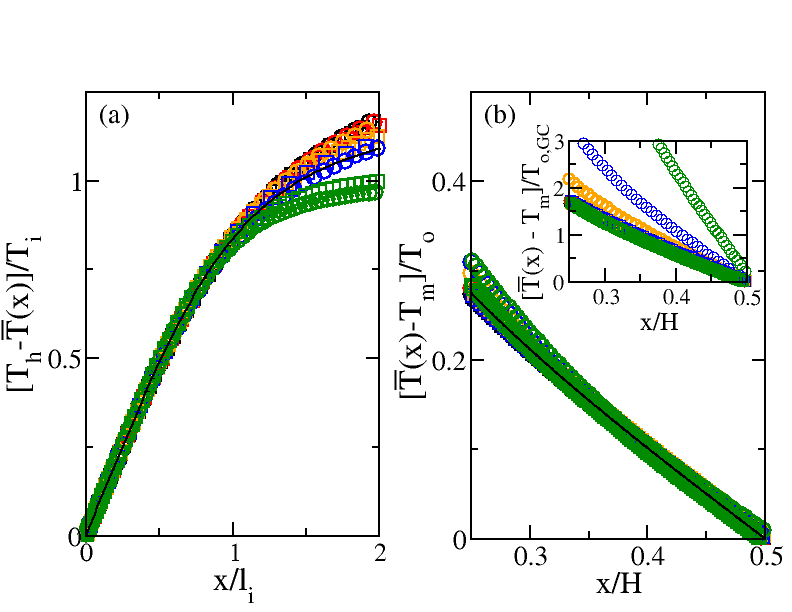
Figure 1: (a) $(T_{h}-\overline{T})/T_{i}$ vs $x/l_{i}$ and (b) $(\overline{T}-T_{m})/T_{o}$ vs $x/H$ at $Ra_{min}$ (circles) and $Ra_{max}$ (squares) for $\Pran=1$ (black), $\Pran=2$ (red), $\Pran=5$ (orange), $\Pran=10$ (blue) and $\Pran=100$ (green). Here, $Ra_{min}$ and $Ra_{max}$ are the minimum and maximum values of $Ra$ for the corresponding $\Pran$ (see table 1). The solid lines in (a) and (b) are $F_{i}$ and $F_{o}$ given by (23) and (24), respectively. In the inset of (b), $(\overline{T}-T_{m})/T_{o,GC}$ is plotted vs $x/H$.

Next we check the validity of (22). As shown in figure 2(b), the rescaling by $T_{o}$ and $l_{o}=H$ results in an approximate collapse of the data in the region $0.3<x/H\leq 0.5$ and the collapsed data are consistent with the outer scaling function $F_{o}$ given by (24). If the outer temperature scale $T_{o,GC}=(q^{2}/\alpha gH)^{1/3}$ proposed by George & Capp (1979) is used instead of $T_{o}$, the data collapse is worse [see the inset of figure 2(b)]. The scale $T_{o,GC}$ was obtained by assuming that the temperature scale in the outer region depends on $q$, $\alpha g$ and $H$ only and not on the molecular diffusivities $\nu$ and $\kappa$. We find that

$$C_{m}\to k_{o}(RaNu)^{1/3}\Pran^{-2/3}$$ (30)

with $k_{o}=0.162$ for sufficiently large $Ra$, which implies that $T_{o}\to k_{o}^{-1}T_{o,GC}$ when $Ra$ is greater than certain threshold value $Ra_{c}(\Pran)$ and $Ra_{c}(\Pran)$ increases with $\Pran$.

We now show that our model gives $Nu\sim Ra^{1/3}$ in the high-$Ra$ limit, in accord with Ching (2023). Using (29) and (30), it can be shown that for sufficiently large $Ra$, $I_{1}(y_{1})\sim(RaNu)^{-1/4}$, $I_{2}(y_{2})\sim(RaNu)^{-1/3}\ln(RaNu)$ and $I_{3}(1/2)\sim(RaNu)^{-1/3}$ and hence

$$Nu\approx\frac{1}{2I_{1}(y_{1})}\Rightarrow Nu\sim Ra^{1/3}.$$ (31)

4.2 Comparison with mean temperature profiles reported in previous studies

One often-cited result was obtained by (George & Capp , 1979). They proposed scaling functions in terms of $T_{i,GC}$, $l_{i,GC}$ and $T_{o,GC}$ and $H$ for the inner and outer regions, respectively. In an overlap layer in which both scaling functions hold, they obtained

$$\frac{T_{h}-\overline{T}(x)}{T_{i,GC}} = -K_{1}\left(\frac{x}{l_{i,GC}}\right)^{-1/3}+\phi_{1}(\Pran),$$ (32)

$$\frac{\overline{T}(x)-T_{m}}{T_{o,GC}} = K_{1}\left(\frac{x}{H}\right)^{-1/3}+\theta_{1}$$ (33)

with undetermined constants $K_{1}$, $\phi(\Pran)$ and $\theta_{1}$; the independence of $K_{1}$ and $\theta_{1}$ on $\Pran$ follows from the independence of the outer scaling function on $\nu$ or $\kappa$. Fitting DNS data for $\Pran=0.709$ (air), Versteegh & Nieuwstadt (1999) and Ng, Chung & Ooi (2013) found $K_{1}=4.2$. Using the DNS data of Howland et al. (2022), we find that the region that (32) with $K_{1}=4.2$ can fit decreases drastically for larger $\Pran$ but (21), rewritten as

$$\frac{T_{h}-\overline{T}(x)}{T_{i,GC}}=g(\Pran)F_{i}\left(\frac{1}{g(\Pran)}\frac{x}{l_{i,GC}}\right),$$ (34)

can give good fits for all the 5 values of $\Pran$ studied. The comparison for $\Pran=1$ and $\Pran=100$ is shown in figure 2.

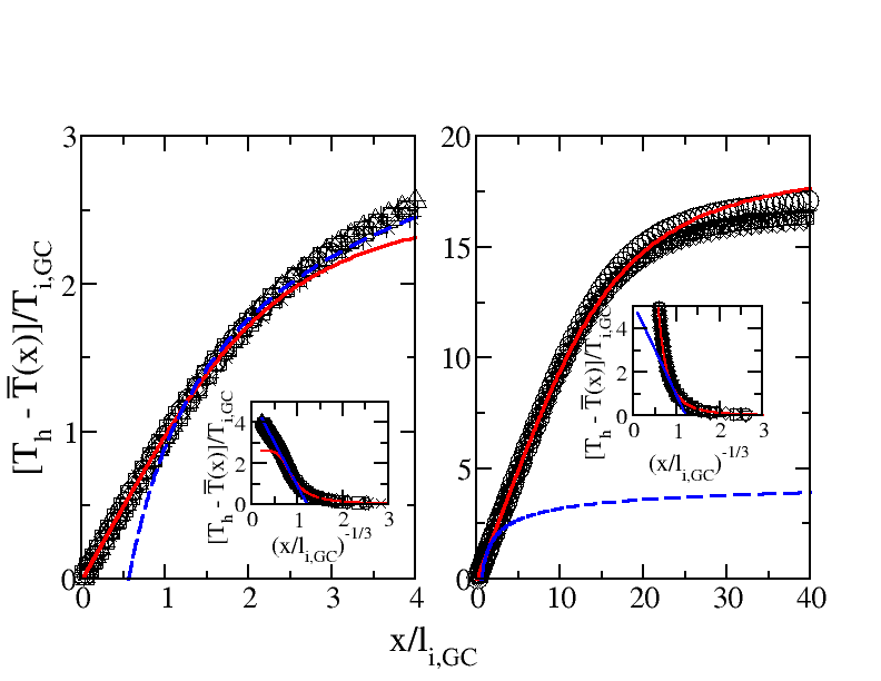
Figure 2: Plots of $[T_{h}-\overline{T}(x)]/T_{i,GC}$ vs $x/l_{i,GC}$ for $\Pran=1$ (left panel) and $\Pran=100$ (right panel) at $Ra=10^{6}$ (plusses), $2\times 10^{6}$ (crosses), $5\times 10^{6}$ (stars), $10^{7}$ (circles), $2\times 10^{7}$ (squares), $5\times 10^{7}$ (diamonds), $10^{8}$ (triangles), $2\times 10^{8}$ (left triangles), $5\times 10^{8}$ (inverted triangles) and $10^{9}$ (right triangles). The red solid lines are (34) and the blue dashed lines are (32) with $K_{1}=4.2$, $\phi_{1}(1)=5.20$ and $\phi_{1}(100)=5.15$.

Using the same approach but with the temperature scale $T_{i,GC}$ for both the inner and outer regions, Hölling & Herwig (2005) obtained a logarithmic profile in the overlap layer:

$$\frac{T_{h}-\overline{T}(x)}{T_{i,GC}} = K_{2}\log\left(\frac{x}{l_{i,GC}}\right)+\phi_{2}(\Pran)$$ (35)

$$\frac{\overline{T}(x)-T_{m}}{T_{i,GC}} = -K_{2}\log\left(\frac{x}{H}\right)+\theta_{2}$$ (36)

with undetermined constants $K_{2}$, $\phi_{2}(\Pran)$ and $\theta_{2}$. Different values of $K_{2}$ and $\phi_{2}$, obtained by fitting DNS data for air, were reported (Versteegh & Nieuwstadt , 1999; Hölling & Herwig , 2005; Kiš & Herwig , 2012; Ng, Chung & Ooi , 2013). We thus test instead the relation between $Nu$, $Ra$ and $\Pran$, obtained by adding (35) and (36) and using (27) and (28):

$$(Nu^{-3}Ra\Pran)^{1/4}=\frac{K_{2}}{2}\log(NuRa\Pran)+2[\phi_{2}(\Pran)+\theta_{2}]$$ (37)

Balaji, Hölling & Herwig (2007) assumed (35) to hold up to $x=H/2$ and obtained a different relation than (37). As shown in figure 3, the DNS data (Howland et al. , 2022) are consistent with (37) with $K_{2}=0$ indicating their incompatibility with (35) and (36). When $K_{2}=0$, (37) reduces to $Nu\sim Ra^{1/3}$.

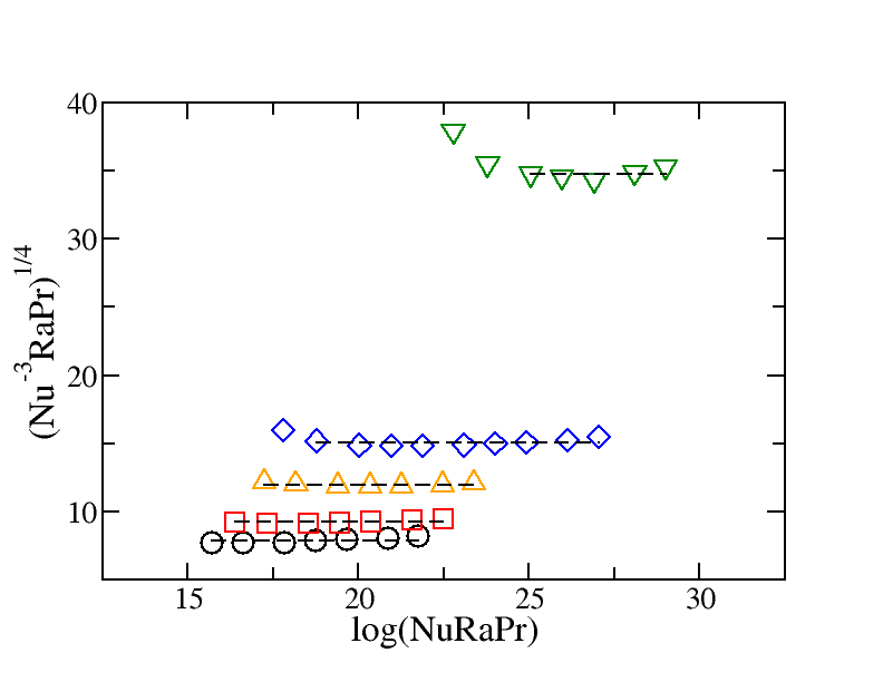
Figure 3: Plot of $(Nu^{-3}Ra\Pran)^{1/4}$ vs $\log(NuRa\Pran)$ for DNS data of Howland et al. (2022).The dashed lines are best fits of (37) with $K_{2}=0$.

5 Conclusions

A three-layer model for the eddy thermal diffusivity has been proposed for turbulent natural convection between two infinite vertical walls at different temperatures. Using this model, analytical results for the mean temperature profile, their two universal scaling functions in the inner layer next to the walls and the outer layer near the centerline between the walls, and the Nusselt number have been derived. Unlike previous studies, the analytical functional forms of the two scaling functions are fully determined and there is no an overlap region in which both functions hold. All our theoretical results have been shown to be in good agreement with DNS data for $1\leq\Pran\leq 100$, obtained by Howland et al. (2022).

[Funding.] This work was funded by the Hong Kong Research Grants Council (Grant No. CUHK 14303623).

[Declaration of interests.] The authors report no conflicit of interest.

[Author ORCIDs.] Ho Yin Ng, https://orcid.org/0009-0003-8811-2743;
Emily S.C. Ching, https://orcid.org/0000-0001-5114-5072