DualHash: A Stochastic Primal-Dual Algorithm with Theoretical Guarantee for Deep Hashing

Abstract

Deep hashing converts high-dimensional feature vectors into compact binary codes, enabling efficient large-scale retrieval. A fundamental challenge in deep hashing stems from the discrete nature of quantization in generating the codes. W-type regularizations, such as $||z|-1|$, have been proven effective as they encourage variables toward binary values. However, existing methods often directly optimize these regularizations without convergence guarantees. While proximal gradient methods offer a promising solution, the coupling between W-type regularizers and neural network outputs results in composite forms that generally lack closed-form proximal solutions. In this paper, we present a stochastic primal-dual hashing algorithm, referred to as DualHash, that provides rigorous complexity bounds. Using Fenchel duality, we partially transform the nonconvex W-type regularization optimization into the dual space, which results in a proximal operator that admits closed-form solutions. We derive two algorithm instances: a momentum-accelerated version with $\mathcal{O}(\varepsilon^{-4})$ complexity and an improved $\mathcal{O}(\varepsilon^{-3})$ version using variance reduction. Experiments on three image retrieval databases demonstrate the superior performance of DualHash.

I Introduction

A key technique in large-scale image retrieval systems is hashing. Image hashing aims to represent the information of an image using a binary code (e.g.,$\pm 1$) for efficient storage and accurate retrieval [1]. Recently, deep learning to hash has shown significant improvements due to its robust feature extraction capability [2, 3], which utilizes neural networks to map high-dimensional feature vectors (e.g., 1024 dimensions) into compact binary codes (e.g., 64 bits). However, a fundamental challenge in deep hashing arises from the discrete nature of quantization. The $sgn$ function used to generate binary codes has zero gradients almost everywhere. This gradient vanishing issue means that standard first-order methods are ineffective in training deep hashing networks [4]. Continuous relaxation methods have been explored to address this issue, but inevitably introduce quantization error: the discrepancy between the optimized continuous values and the final discrete values [5].

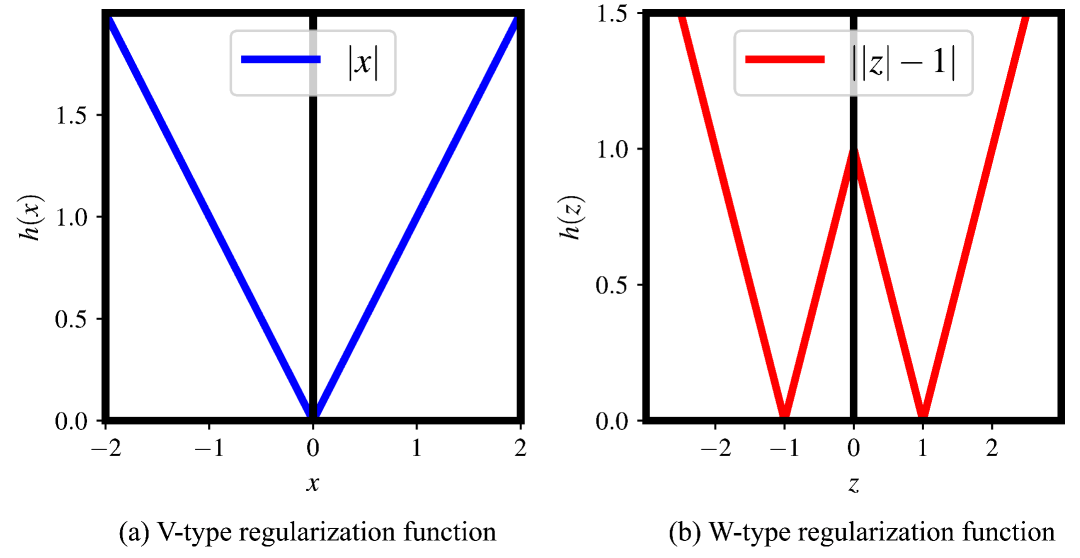
Figure 1: The V-type (left) versus W-type (right) regularizations.

To mitigate this issue, researchers have developed specialized regularization techniques [6, 7, 8]. Among them, W-type regularizations, such as $||z|-1|$, have proven effective. These regularizers impose sharp penalties to encourage variables towards binary values (e.g., $-1$ or $1$). Mathematically, this approach naturally formulates deep hashing as a nonconvex composite optimization problem:

$$\min_{\bm{x}\in\mathcal{X}}\quad\frac{1}{n}\sum_{i=1}^{n}f_{i}(\bm{x})+\sum_{i=1}^{n}h(\bm{D}_{i}(\bm{x})),$$ (I.1)

where $f_{i}$ and $\bm{D}_{i}$ are continuously differentiable and $h$ is a proper and lower semi-continuous (l.s.c.) regularizer.

Regularization techniques are widely used in machine learning and deep learning to encourage desirable model structures [9, 10, 11]. Classic examples include the $\ell_{1}$ norm to introduce sparsity [12] and the $\ell_{2}$ norm weight decay to prevent overfitting [13]. In practice, researchers typically apply stochastic (sub)gradient methods (SGD) directly [14, 15] to optimize the objective, and deep hashing follows this paradigm as well [4, 16, 17]. This seemingly effective choice, however, frequently leads to suboptimal performance. The regularizer is often nonsmooth around some regions; using subgradients may result in slow convergence and oscillation.

A powerful tool to circumvent the nonsmoothness of a regularizer is via its proximal operator. Proximal-based methods thus offer a promising solution for composite optimization [18]. For a regularized deep network with $\bm{D}_{i}(\bm{x})=\bm{x}$ in (I.1), stochastic proximal gradient methods (SPGD) have been extensively studied [19, 20, 21, 22, 23]. Recently, [24] has established global convergence of SPGD for the $\ell_{1}$ regularized model and [25] has presented a unified adaptive SPGD framework with $\mathcal{O}(\varepsilon^{-4})$ complexity for l.s.c. regularizations. However, these excellent methods crucially rely on regularizers with tractable proximal solutions, such as the well-known soft-thresholding operator of $\ell_{1}$ norm (Figure˜1(a)). In contrast, while the W-type regularization (Figure˜1(b)) admits a closed-form proximal operator [26], their composition with neural network outputs (i.e., $h(\bm{D}_{i}(\bm{x}))$, which is typically highly nonconvex, creates a computationally intractable subproblem. This renders SPGD impractical for the problem (I.1).

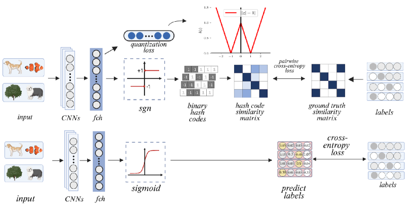
Figure 2: Comparison between deep learning for hashing and classification

In fact, the nonlinear composite form $h(\bm{D}_{i}(\bm{x}))$ presents a unique requirement in deep hashing, as the application of regularization in this field fundamentally differs from that in standard networks. We demonstrate this distinction by comparing with a basic classification task in Figure˜2. While classification directly employs network outputs for prediction, deep hashing requires generating binary hash codes for downstream retrieval tasks. This unique requirement leads to W-type regularization, which typically constrains the final network output rather than focusing on parameter properties. Therefore, it is necessary to explicitly consider the nonlinear composite form.

Recent works [27, 28, 29, 30] have addressed compositional structures similar to (I.1), which ensure either weak convexity of $h(\bm{D}_{i})$ or convexity on $h$. Other studies [31, 32] focus on stochastic optimization with linear compositional structures. On the contrary, our model faces a more challenging scenario where $h$ is nonconvex with a nonlinear composition that implies $h(\bm{D}_{i})$ is not weakly convex. [33] considers the problem (I.1) in deterministic setting. They converted it to a constrained optimization problem and established an asymptotic convergence via the Lagrangian-based method. However, their analysis does not provide non-asymptotic complexity guarantees for the stochastic case in deep hashing.

In this paper, we propose an efficient deep hashing algorithm to address these challenges posed by nonlinear composition with W-type regularization. Our approach presents a reformulation of the W-type regularized problem using a decouple scheme and designs a new primal-dual algorithm using Fenchel duality. We aim to bridge the theoretical-practical gap by providing rigorous non-asymptotic convergence analysis and enhanced practical performance in deep hashing. Our main contributions are as follows:

• We reformulate deep hashing models with the W-type regularization into a two-block finite-sum optimization problem. This reformulation decouples the challenging $h(\bm{D}(\bm{x}))$, simplifying the sequential analysis.

• Building on this problem, we propose DualHash, a stochastic primal-dual deep hashing algorithm. Using Fenchel duality, we partially transform the nonconvex W-type regularization optimization into a convex dual formulation that admits closed-form updates, ensuring robustness and stable convergence. To incorporate numerical acceleration, we develop two important instances: a momentum-based implementation (DualHash-StoM) and a variance-reduced implementation using STORM (DualHash-StoRM).

• We provide rigorous non-asymptotic complexity analysis for deep hashing optimization. Specifically, we establish an $\mathcal{O}(\varepsilon^{-4})$ complexity bound for DualHash-StoM and an improved optimal $\mathcal{O}(\varepsilon^{-3})$ complexity bound for DualHash-StoRM. Table I summarizes how our work compares to previous deep hashing methods.

• Extensive experiments on three standard datasets demonstrate the practical effectiveness of DualHash. In particular, our proposed method achieves consistently lower quantization errors across different bit lengths compared to baselines, validating the advantages of our primal-dual framework.

I-A Related Work

Optimization in deep hashing. Modern deep hashing methods have developed two main strategies: continuous relaxation and discrete optimization schemes. Continuous relaxation methods use smooth activation functions and mitigate quantization error by incorporating explicit regularization terms, such as W-type functions [8, 17, 34]. Other approaches explore unified formulations through single-objective continuous optimization [4, 16]. These algorithms use stochastic (adaptive) gradient methods to optimize the objective. Alternative strategies directly address binary constraints by introducing auxiliary hash codes [35, 7, 36]. Please refer to Table˜I for a comparison.

Primal-Dual and ADMM Methods for Nonconvex Optimization. From a constrained optimization perspective, Problem (I.1) can be reformulated using auxiliary variables, leading to a nonlinearly constrained problem. There has been growing interest in primal-dual methods for such problems, particularly augmented Lagrangian methods (ALM) and their stochastic variants. A Lagrangian-based framework was pioneered for deterministic settings by [33]. This line of work was subsequently extended to stochastic settings in [37, 38, 39], which primarily address single-block problem structures. This type of block-separable structure is naturally amenable to the Alternating Direction Method of Multipliers (ADMM), a technique that decomposes complex problems into simpler subproblems. Originally developed for convex optimization [40], ADMM has well-established convergence guarantees and complexity analyses in the convex setting [41, 42]. Driven by its empirical success in nonconvex applications such as neural network training [43], nonconvex ADMM and its associated complexity analysis have attracted significant research attention [44, 45, 46, 47]. Notably, [48] provided a pioneering analysis that established gradient (or sample) complexity bounds for nonconvex stochastic ADMM.

TABLE I: Comparison of optimization and convergence guarantee of deep hashing methods.

Type	Method	Model	Quantization Loss	Optimization	Complexity
Discrete	DDSH [35]	$\min L_{s}(\bm{b})+Q(\bm{u},\bm{b})$	$\|\cdot\|^{2}$	BQP	$-$
	DSDH [7]	$\min L_{s}(\bm{u})+Q(\bm{u},\bm{b})$	$\|\cdot\|^{2}$	$sgn$ update
	DPSH [36]			DCC
Continuous	DCH [6]	$\min L_{s}(\bm{u})+h(\bm{u})$	$\log\left(1+\frac{\text{dist}_{\text{h}}(|\bm{u}|,\mathbf{1})}{\gamma}\right)$	SGDM
	DNNH [49]		$\mathcal{I}_{[-1,1]^{d}}(\bm{u})$
	DSH [8]		$\||\bm{u}|-\mathbf{1}\|_{1}$
	DTSH [50]		$\||\bm{u}|-\mathbf{1}\|_{2}^{2}$
	DHN [34]		$\sum_{i}\log(\cosh(|u_{i}|-1))$
	MDSHC [17]	$\min L_{c}(\bm{u})+L_{s}(\bm{u})+h(\bm{u})$	$\||\bm{u}|-\mathbf{1}\|_{1}$	RMSProp
	HashNet [4]	$\min L_{s}(\bm{u})$	-	SGDM
	OrthoHash [16]			Adam
	DualHash-StoM	$\min L_{s}(\bm{u})+Q(\bm{u},\bm{b})+h(\bm{b})$	$\||\bm{b}|-\mathbf{1}\|_{1}$	Sto Primal-Dual	$\mathcal{O}(\varepsilon^{-4})$
	DualHash-StoRM				$\mathcal{O}(\varepsilon^{-3})$

Notes: The Type column indicates whether the method uses discrete or continuous optimization for quantization. The Model column shows the core optimization objective, where $\bm{b}$ denotes binary codes and $\bm{u}$ denotes continuous outputs. The Quantization Loss column specifies the loss ($Q(\cdot,\cdot)$ or $h(\cdot)$) for quantization error, with ‘-’ indicating no explicit loss. The Optimization column describes the training strategy, with discrete methods focusing on binary code updates. DCC stands for Discrete Cyclic Coordinate, while BQP denotes Binary Quadratic Programming. The Complexity column reports the convergence rate, with ‘-’ indicating no such analysis.

II Preliminary

Notations. We use $a$, $\bm{a}$, and $\bm{A}$ to denote scalars, vectors, and matrices, respectively. Throughout this paper, $\bm{1}$ represents a vector of all ones, and $i,j$ serve as indices. Let $\mathcal{X},\mathcal{B},\mathcal{Y}$ be finite-dimensional real Hilbert spaces equipped with inner product $\langle\cdot,\cdot\rangle$ and induced norm $\|\cdot\|:=\sqrt{\langle\cdot,\cdot\rangle}$. Unless specified otherwise, $\|\cdot\|$ denotes the Euclidean norm for vectors and the Frobenius norm for matrices. We use $\mathcal{X}^{*},\mathcal{B}^{*},\mathcal{Y}^{*}$ to represent the dual spaces. $|\cdot|$ denotes element-wise absolute value. For a closed set $\mathcal{C}\subseteq\mathcal{X}$, the distance from a point $\bm{x}\in\mathcal{X}$ to $\mathcal{C}$ is defined as $\text{dist}(\bm{x},\mathcal{C}):=\min_{\bm{y}\in\mathcal{C}}\|\bm{x}-\bm{y}\|$.

The extended real-valued function $f:\mathbb{R}^{q}\rightarrow(-\infty,+\infty]$ is called proper if its domain $\text{dom}(f):=\{\bm{x}\in\mathcal{X}\mid f(\bm{x})<+\infty\}$ is nonempty and $\inf\limits_{\bm{x}\in\mathbb{R}^{q}}f>-\infty$; it is closed if its epigraph $\text{epi}(f):=\left\{(\bm{x},t)\in\mathbb{R}^{q+1}\mid f(\bm{x})\leq t\right\}$ is closed. For a proper, closed, and convex function $f$, the proximal mapping of $f$, denoted by $\operatorname{prox}_{\tau f}(\bm{y})$, is defined as

$$\operatorname{prox}_{\tau f}(\bm{y}):=\operatorname*{\mathrm{argmin}}\limits_{\bm{x}\in\operatorname{dom}(f)}\left\{f(\bm{x})+\frac{1}{2\tau}\|\bm{x}-\bm{y}\|^{2}\right\},$$ (II.1)

where $\tau$ is a positive scalar parameter.

A function $f:\mathcal{X}\rightarrow\mathbb{R}$ is said to be $L_{f}$-smooth if $\|\nabla f(\bm{x})-\nabla f(\bm{x}^{\prime})\|\leq L_{f}\|\bm{x}-\bm{x}^{\prime}\|$ for all $\bm{x},\,\bm{x}^{\prime}\in\mathbb{R}^{n}$. A mapping $\mathcal{M}:\mathcal{D}\to\mathbb{R}^{l}$ is said to be $C$-Lipschitz continuous if $\|\mathcal{M}(\bm{x})-\mathcal{M}(\bm{x}^{\prime})\|\leq C\|\bm{x}-\bm{x}^{\prime}\|$ for all $\bm{x},\bm{x}^{\prime}\in\mathcal{D}$. A well-known gradient descent lemma for a smooth function is that

$$f(\bm{x})\leq f(\bm{x}^{\prime})+\langle\nabla f(\bm{x}^{\prime}),\bm{x}-\bm{x}^{\prime}\rangle+\frac{L_{f}}{2}\|\bm{x}-\bm{x}^{\prime}\|^{2}.$$ (II.2)

III Problem reformulation

III-A W-type Regularized Deep Hashing Model

Deep hashing methods aim to learn network parameters $\bm{x}\in\mathcal{X}\subseteq\mathbb{R}^{d_{\bm{x}}}$ to generate discrete codes that preserve semantic similarity effectively in the Hamming space. A natural approach is to minimize a similarity-preserving loss function $\frac{1}{n}\sum_{i=1}^{n}L_{s}(\text{sgn}(\bm{C}_{i}(\bm{x})))$ where $n$ is the number of training samples, $\bm{C}_{i}(\bm{x})$ represents the $i$-th network output and $f_{i}$ is the similarity-preserving loss function (e.g., pairwise cross-entropy loss [34]). However, the function $sgn(\cdot)$ renders standard backpropagation infeasible due to its zero gradient for all nonzero inputs. This discreteness poses a central challenge in deep hashing.

A W-type regularization (e.g., $\lambda||z|-1|$) has effectively mitigated this issue. This type of regularization encourages outputs to approach binary values $\{-1,1\}$ during training. Specifically, the model is trained to produce continuous outputs $\bm{u}_{i}=\bm{D}_{i}(\bm{x})$ with W-type regularization, and binary codes are obtained post-training via $\bm{b}_{i}=\text{sgn}(\bm{u}_{i})$. Consequently, we formulate the core optimization problem for W-type regularized deep hashing methods as follows,

$$\min_{\bm{x}\in\mathcal{X}}\quad\frac{1}{n}\sum_{i=1}^{n}f_{i}(\bm{x})+\sum_{i=1}^{n}h(\bm{D}_{i}(\bm{x})),$$ (III.1)

where $\frac{1}{n}\sum_{i=1}^{n}f_{i}$ is the similarity-preserving loss, $D_{i}$ is the $i$-th network output and $h$ is a W-type regularization.

III-B A Two-Block Structured Reformulation

We then employ variable splitting to reformulate problem (III.1) equivalently as the constrained problem:

$$\min_{\bm{x}\in\mathcal{X},\bm{B}\in\mathcal{B}} \quad\frac{1}{n}\sum_{i=1}^{n}f_{i}(\bm{x})+\sum_{i=1}^{n}h(\bm{b}_{i})$$

s.t. $$\quad\bm{b}_{i}=\bm{D}_{i}(\bm{x}),\;\forall i=1,\dots,n.$$ (III.2)

Combined with the quadratic penalty method [51], this transformation yields the following two-block finite-sum optimization problem:

$$\min_{\bm{x}\in\mathcal{X},\bm{B}\in\mathcal{B}}J(\bm{x},\bm{B})$$

$$=\overbrace{\underbrace{\frac{1}{n}\sum_{i=1}^{n}f_{i}(\bm{x})}_{f(\bm{x})}+\underbrace{\frac{\gamma}{2n}\sum_{i=1}^{n}\|\bm{D}_{i}(\bm{x})-\bm{b}_{i}\|^{2}}_{P(\bm{x},\bm{B})}}^{F(\bm{x},\bm{B})=\frac{1}{n}\sum_{i=1}^{n}F_{i}(\bm{x},\bm{b}_{i})}+\underbrace{\sum_{i=1}^{n}h(\bm{b}_{i})}_{h(\bm{B})}.$$ (P)

Here, $\bm{B}=[\bm{b}_{1},\bm{b}_{2},\dots,\bm{b}_{n}]$ and $\gamma>0$ is the penalty parameter. This reformulation decomposes the original problem (III.1) into simpler structural blocks, enabling us to exploit the problem structure better. Building upon this problem, we develop a stochastic primal-dual algorithm that effectively addresses the challenges above.

IV Algorithm

IV-A DualHash: A Stochastic Primal-Dual Hashing Algorithm

Inspired by PDHG [52] in convex optimization and its nonconvex extension PPDG [53], we consider the equivalent constrained formulation of the problem (III-B):

$$\min_{\bm{x}\in\mathcal{X},\bm{B}\in\mathcal{B},\bm{y}\in\mathcal{Y}} \quad F(\bm{x},\bm{B})+h(\bm{Y})$$

s.t. $$\quad\bm{Y}=\bm{B},$$

whose corresponding dual problem is

$$\max_{\bm{\Lambda}\in\mathcal{Y}^{*}}\min_{\bm{x}\in\mathcal{X},\bm{B}\in\mathcal{B},\bm{y}\in\mathcal{Y}} \quad F(\bm{x},\bm{B})+h(\bm{Y})+\langle\bm{\Lambda},\bm{B}-\bm{Y}\rangle.$$ (D)

Recalling the definition of the conjugate function [54]:

$$h^{*}(\bm{Y}):=\sup_{\bm{x}\in\mathcal{Y}}\{\langle\bm{Y},\bm{x}\rangle-h(\bm{x})\},\quad\bm{Y}\in\mathcal{Y}^{*},$$

and observing that the minimization with respect to $\bm{Y}$ in the problem (D) can be performed independently, we then simplify the Lagrangian function in the problem (D) to

$$\mathcal{L}(\bm{x},\bm{B},\bm{\Lambda}):=F(\bm{x},\bm{B})+\langle\bm{B},\bm{\Lambda}\rangle-h^{*}(\bm{\Lambda}). \mathcal{L}$$ ()

Through this transformation, we replace $h(\bm{Y})$ with $-h^{*}(\bm{\Lambda})$ and can optimize $h^{*}$ in the dual space. Since $h^{*}$ is always convex and l.s.c. [54], it means that the $\text{prox}_{h^{*}}(\cdot)$ is often much easier to compute (potentially having a closed-form solution) than that of $h$. For $h(\bm{z})=\sum_{i=1}^{n}\lambda||z_{i}|-1|$, we derive its conjugate function as illustrated in Figure˜3:

$$h^{*}(\bm{x})=\sum_{i=1}^{n}h^{*}(x_{i}),\,\,$$

$$\text{where }h^{*}(x_{i})=\begin{cases}|x_{i}|,&\text{if }x_{i}\in[-\lambda,\lambda],\\ +\infty,&\text{otherwise},\end{cases}$$

whose proximal operator in the piecewise solution is

$$[\operatorname{prox}_{\tau h^{*}}(\bm{y})]_{i}=\begin{cases}\lambda,&y_{i}>\lambda+\tau,\\ y_{i}-\tau,&\tau<y_{i}\leq\lambda+\tau,\\ 0,&-\tau\leq y_{i}\leq\tau,\\ y_{i}+\tau,&-\lambda-\tau\leq y_{i}<-\tau,\\ -\lambda,&y_{i}<-\lambda-\tau.\end{cases}$$ (IV.1)

This motivates us to perform a proximal step to update $\bm{\Lambda}$.

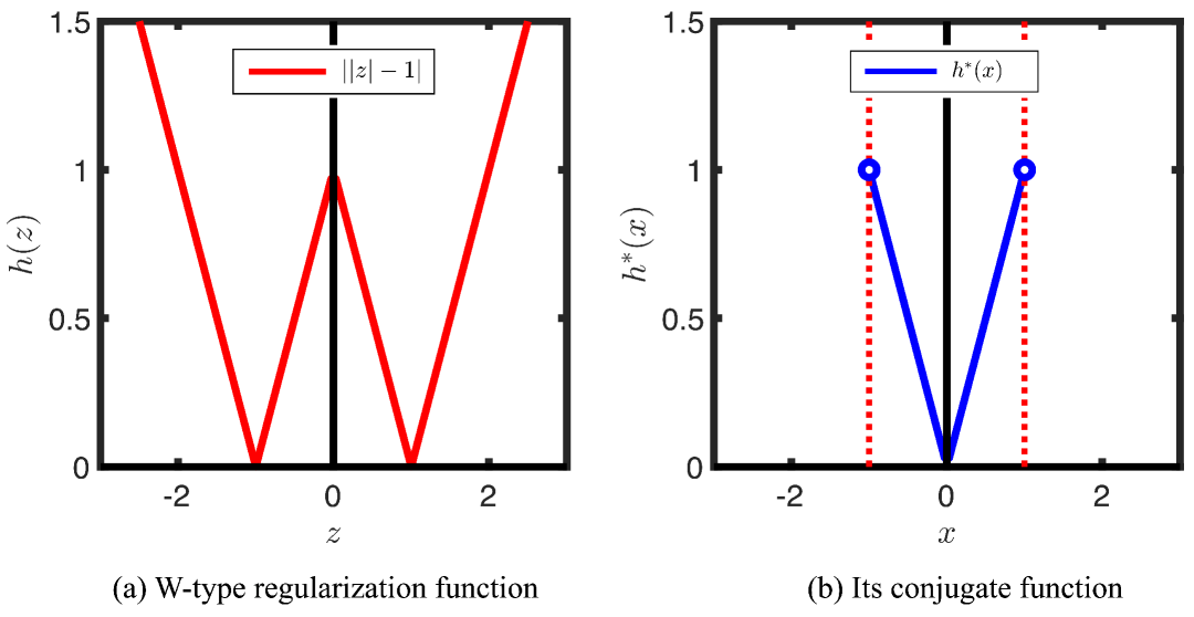
Figure 3: W-type regularization function $h(z)=\lambda||z|-1|$ and its conjugate function $h^{*}(x)$.

We now outline DualHash, which employs an alternating update scheme for $\bm{x},\bm{B},\bm{\Lambda}$. we adopt a stochastic first-order method for the $\bm{x}$-update since computing the full gradient $\nabla_{\bm{x}}F(\bm{x},\bm{B})$ is computationally expensive for typically the large number of samples $n$ in deep learning. Specifically, at each iteration $k$, we uniformly sample a mini-batch $\mathcal{J}_{k}\subseteq\{1,\cdots,n\}$ with $b_{k}=|\mathcal{J}_{k}|\leq n$ and compute:

$$\nabla_{\bm{x}}F(\bm{x}^{k},\bm{B}^{k};\mathcal{J}_{k})=\,\frac{1}{|\mathcal{J}_{k}|}\sum_{j\in\mathcal{J}_{k}}\nabla_{\bm{x}}F_{j}(\bm{x}^{k},\bm{b}_{j}^{k}).$$ (IV.2)

Then we utilize this approximation within an optimization strategy chosen to enhance efficiency (e.g., incorporating momentum or variance reduction), as detailed in Section˜IV-B. Second, the auxiliary variable $\bm{B}$ is updated via a simple gradient descent step (IV.3); this suffices because the objective ($\mathcal{L}$) with respect to $\bm{B}$ is smooth with an inexpensive gradient,

$$\bm{B}^{k+1} =\bm{B}^{k}-\tau\nabla_{\bm{B}}\mathcal{L}(\bm{x}^{k+1},\bm{B}^{k},\bm{\Lambda}^{k})$$

$$=\bm{B}^{k}-\tau\left(\nabla_{\bm{B}}F(\bm{x}^{k+1},\bm{B}^{k})+\bm{\Lambda}^{k}\right).$$ (IV.3)

Finally, the dual variable $\bm{\Lambda}$ is updated via proximal gradient ascent on $h^{*}$, using an extrapolation step introduced in [52]. The update solves the following optimization problem:

$$\bm{\Lambda}^{k+1} =\text{prox}_{(1/\tau h^{*})}\left(\bm{\Lambda}^{k}+\left(2\bm{B}^{k+1}-\bm{B}^{k}\right)\right)$$

$$=\arg\min_{\bm{\Lambda}\in\mathcal{Y}^{*}}\left\{h^{*}(\bm{\Lambda})-\langle\bm{\Lambda},2\bm{B}^{k+1}-\bm{B}^{k}\rangle\right.$$

$$\quad\quad\quad\quad\quad\quad\quad\quad\quad\quad\left.+\frac{\tau}{2}\|\bm{\Lambda}-\bm{\Lambda}^{k}\|^{2}\right\}.$$ (IV.4)

IV-B Implementations

The unified DualHash framework allows for flexible choices in the $\bm{x}$ update step based on a mini-batch stochastic gradient approximation (IV.2). This flexibility enables us to incorporate advanced stochastic optimization techniques. We thus instantiate the $\bm{x}$-update using two well-established approaches: momentum [55, 56] and variance reduction [57], which can improve empirical training efficiency and can also improve the theoretical convergence guarantees [58, 59].

DualHash-StoM The heavy ball method [60] and Nesterov acceleration [55] can be integrated with stochastic gradient descent (SGD) to yield accelerated variants like SGD with momentum, which significantly speeds up convergence. This approach has become a popular strategy for training neural networks [61, 62]. We thus incorporate this technique and compute the stochastic gradient estimator (Line 3 of Algorithm˜1) as:

$$\bm{G}^{k}=\nabla_{\bm{x}}F(\bm{z}^{k},\bm{B}^{k};\mathcal{J}_{k}),\,\text{where }\bm{z}^{k}=\bm{x}^{k}+\beta_{k}(\bm{x}^{k}-\bm{x}^{k-1}).$$ (IV.5)

The update of $\bm{x}^{k}$ (Line 4 of Alg. 1) is then:

$$\bm{x}^{k+1}=\bm{y}^{k}-\eta_{k}\bm{G}^{k},\,\text{where }\bm{y}^{k}=\bm{x}^{k}+\alpha_{k}(\bm{x}^{k}-\bm{x}^{k-1}).$$ (IV.6)

The overall algorithm, DualHash-StoM, is detailed in Algorithm˜1.

Remark IV.1

The momentum acceleration framework in (IV.6) covers these two accelerations: Nesterov acceleration [55] corresponds to $\alpha_{k}=\beta_{k}\neq 0$; the heavy-ball method [60] is obtained with $\beta_{k}=0$; vanilla SGD is recovered when $\alpha_{k}=\beta_{k}=0$; In this paper, we set $\alpha_{k},\beta_{k}\in(0,1)$ for all $k\geq 1$.

DualHash-StoRM Alternatively, we employ the STORM estimator [63] for the $\bm{x}$-update. STORM utilizes a recursive momentum mechanism to reduce gradient variance, which is motivated by SGDM. Unlike some other variance reduction techniques (e.g., SVRG [64], SARAH [65]) that require full-gradient or large-batch gradient computations, STORM achieves variance reduction without such requirements. Given its practical effectiveness in deep learning [63, 66], we compute the stochastic gradient estimator (Line 3 of Algorithm˜2) as:

$$\bm{D}^{k}=\begin{cases}\nabla_{\bm{x}}F(\bm{x}^{1},\bm{B}^{1};\mathcal{J}_{1}),&\text{if }k=1,\\ (1-\rho_{k-1})\big(\bm{D}^{k-1}-\nabla_{\bm{x}}F(\bm{x}^{k-1},\bm{B}^{k-1};\mathcal{J}_{k-1})\big)\\ +\nabla_{\bm{x}}F(\bm{x}^{k},\bm{B}^{k};\mathcal{J}_{k}),&\text{if }k>1.\end{cases}$$ (IV.7)

The update of $\bm{x}$ (Line 4 of Algorithm˜2) is then

$$\bm{x}^{k+1}=\bm{x}^{k}-\eta_{k}\bm{D}^{k}.$$ (IV.8)

The overall algorithm, DualHash-StoRM, is detailed in Algorithm˜2.

Algorithm 1 DualHash-StoM

1:  Initialize: $\bm{x}^{1}=\bm{z}^{1}=\bm{y}^{1}\in\mathcal{X}$, $\bm{B}^{1}\in\mathcal{B},\,\bm{\Lambda}^{1}\in\mathcal{Y}^{*}$, parameters $\{\eta_{k}\}$, $\tau$, $b_{k}$, $\{\alpha_{k},\beta_{k}\in(0,1)\}$

2:  for $k=1,2,\ldots$ do

3:   Compute $\bm{G}^{k}$ by (IV.5)

4:   Update $\bm{x}^{k+1}$ by (IV.6)

5:   Update $\bm{B}^{k+1}$ by (IV.3)

6:   Update $\bm{\Lambda}^{k+1}$ by (IV.4)

7:  end for

8:  Return: $\bm{x}_{R}$ where $R$ is uniformly sampled from $\{2,\ldots,T+1\}$

Algorithm 2 DualHash-StoRM

1:  Initialize: $\bm{x}^{1}\in\mathcal{X}$, $\bm{B}^{1}\in\mathcal{B},\,\bm{\Lambda}^{1}\in\mathcal{Y}^{*}$, parameters $\{\eta_{k}\}$, $\tau$, $b_{k}$, $\{\rho_{k}\in(0,1)\}$

2:  for $k=1,2,\ldots$ do

3:   Compute $\bm{D}^{k}$ by (IV.7)

4:   Update $\bm{x}^{k+1}$ by (IV.8).

5:   Update $\bm{B}^{k+1}$ by (IV.3).

6:   Update $\bm{\Lambda}^{k+1}$ by (IV.4).

7:  end for

8:  Return: $\bm{x}_{R}$ where $R$ is uniformly sampled from $\{2,\ldots,T+1\}$

Remark IV.2

The update steps for $\bm{B}$ and $\bm{\Lambda}$ imply the following optimality conditions, which may result in explicit closed-solution in deep hashing. The $\bm{B}$-update in (IV.3) yields:

$$\bm{B}^{k}=\bm{B}^{k-1}-\tau\left(\nabla_{\bm{B}}F(\bm{x}^{k},\bm{B}^{k-1})+\bm{\Lambda}^{k-1}\right).$$ (IV.9)

For the $\bm{\Lambda}$-update in (IV.4), the proximal operator definition gives:

$$\tau\left(\bm{\Lambda}^{k}+\tau^{-1}(2\bm{B}^{k}-\bm{B}^{k-1})-\bm{\Lambda}^{k}\right)\in\partial h^{*}(\bm{\Lambda}^{k}),$$

which is equivalent to the existence of $\mathcal{G}_{\bm{\Lambda}}^{k}\in\partial h^{*}(\bm{\Lambda}^{k})$ such that:

$$\mathcal{G}_{\bm{\Lambda}}^{k}=(2\bm{B}^{k}-\bm{B}^{k-1})+\tau(\bm{\Lambda}^{k-1}-\bm{\Lambda}^{k}).$$ (IV.10)

If the sequence $\{(\bm{x}^{k},\bm{B}^{k},\bm{\Lambda}^{k})\}$ converges to $(\bm{x}^{*},\bm{B}^{*},\bm{\Lambda}^{*})$, then by the outer semicontinuity of $\partial h^{*}(\cdot)$, we have $\bm{B}^{*}\in\partial h^{*}(\bm{\Lambda}^{*})$. This establishes (V.4), which is precisely the necessary condition for the second relation in (V.2).

V Complexity analysis

We now investigate the complexity analysis for DualHash-StoM (Algorithm˜1) and DualHash-StoRM (Algorithm˜2). Our objective is to find an approximate stochastic critical point of the Lagrangian function ($\mathcal{L}$), i.e., a point satisfying

$$\mathbb{E}[\text{dist}^{2}(\bm{0},\partial\mathcal{L}(\bm{x}^{*},\bm{B}^{*},\bm{\Lambda}^{*}))]\leq\varepsilon^{2}$$ (V.1)

for a given $\varepsilon>0$. We assume in this paper the set $\text{crit}\mathcal{L}:=\{(\bm{x}^{*},\bm{B}^{*},\bm{\Lambda}^{*})\in\mathcal{X}\times\mathcal{B}\times\mathcal{Y^{*}}:\bm{0}\in\partial\mathcal{L}(\bm{x}^{*},\bm{B}^{*},\bm{\Lambda}^{*})\}$ is nonempty. This focus is standard in non-convex stochastic optimization analysis, as finding a global or even local minimizer for non-convex optimization problems is generally NP-hard. In particular, we can prove that a critical point of the Lagrangian function ($\mathcal{L}$) is a first-order necessary optimal condition of problem (III-B) as follows.

Lemma 1

Suppose that $\min\limits_{\bm{x},\bm{B}}\mathcal{L}(\bm{x},\bm{B},\bm{\Lambda})>-\infty$ and $(\bm{x}^{*},\bm{B}^{*},\bm{\Lambda}^{*})$ are the optimal solutions of the problem (III-B) and the problem (D), respectively. Then, it holds that $(\bm{x}^{*},\bm{B}^{*},\bm{\Lambda}^{*})\in\text{crit}\mathcal{L}$, i.e., $\bm{0}\in\partial\mathcal{L}(\bm{x}^{*},\bm{B}^{*},\bm{\Lambda}^{*})$.

Proof 1

According to [67, Theorem 2.158], $(\bm{x}^{*},\bm{B}^{*},\bm{\Lambda}^{*})$ are optimal solutions to the primal problem (III-B) and the dual problem (D) if and only if:

$$\begin{cases}(\bm{x}^{*},\bm{B}^{*})\in\operatorname*{\mathrm{argmin}}\limits_{\bm{x}\in\mathcal{X},\bm{B}\in\mathcal{B}}\mathcal{L}(\bm{x}^{*},\bm{B}^{*},\bm{\Lambda}^{*}),\\ 0=h(\bm{B}^{*})+h^{*}(\bm{\Lambda}^{*})-\langle\bm{\Lambda}^{*},\bm{B}^{*}\rangle.\end{cases}$$ (V.2)

The first condition in (V.2) implies that $\bm{0}$ belongs to the subdifferential of $\mathcal{L}$ with respect to $(\bm{x},\bm{B})$ at $(\bm{x}^{*},\bm{B}^{*},\bm{\Lambda}^{*})$. Since $\mathcal{L}$ is continuously differentiable in $(\bm{x},\bm{B})$, we have

$$\begin{cases}\bm{0}&=\nabla f(\bm{x}^{*})+\nabla_{\bm{x}}G(\bm{x}^{*},\bm{B}^{*}),\\ \bm{0}&=\nabla_{\bm{B}}G(\bm{x}^{*},\bm{B}^{*})+\bm{\Lambda}^{*}.\end{cases}$$ (V.3)

For the second condition in (V.2), by the definition of the conjugate function, if this equality holds, then $\bm{\Lambda}^{*}$ is the optimal solution of $\sup\{\left<\bm{b}^{*},\bm{\lambda}\right>-h^{*}(\bm{\lambda})\}$, i.e.,

$$\bm{B}^{*}\in\partial h^{*}(\bm{\Lambda}^{*}).$$ (V.4)

Combining (V.3) and (V.4), we obtain $\bm{0}\in\partial\mathcal{L}(\bm{x}^{*},\bm{B}^{*},\bm{\bm{\Lambda}}^{*})$, completing the proof. $\square$

We then make the following assumptions generally used in stochastic optimization [68, 69, 21].

Assumption 1

• We assume that the sequences $\{(\bm{x}^{k},\bm{B}^{k},\bm{\Lambda}^{k})\}_{k\in\mathbb{N}}$ generated by Algorithms 1 and 2 are bounded. Moreover, the objective of (III-B) is lower bounded by $J^{*}$.

• We assume that $F(\bm{x},\bm{B})$ is $L_{F}$-smooth with respect to $(\bm{x},\bm{B})$, where $L_{F}=\mathcal{O}\left(1\right)$.

• Suppose index $i\sim\text{Uniform}\{1,\ldots,n\}$. For any $\bm{B}\in\mathcal{B}$, there exists a constant $\sigma^{2}\geq 0$ such that $\mathbb{E}_{i}[\nabla_{\bm{x}}F_{i}(\bm{x},\bm{b}_{i})]=\nabla_{\bm{x}}F(\bm{x},\bm{B})$ and $\mathbb{E}_{i}[\|\nabla_{\bm{x}}F_{i}(\bm{x},\bm{b}_{i})-\nabla_{\bm{x}}F(\bm{x},\bm{B})\|^{2}]\leq\sigma^{2}$.

Remark V.1

1. The boundedness in ˜1 (i) is maintained in practice for each variable: $\bm{\Lambda}^{k}$ remains bounded due to its proximal update rule (IV.4) for $\bm{\Lambda}^{k}$ with the truncation property of $\text{prox}_{h^{*}}$ in (IV.1); The $\bm{B}^{k}$ naturally converges toward $\pm 1$ through W-type regularization; and network parameters $\bm{x}^{k}$ are stabilized via weight decay and pretrained initialization, ensuring objective coercivity.

2. The smoothness constant $L_{F}$ remains $\mathcal{O}(1)$, as the penalty formulation is designed to cancel the potential $\mathcal{O}(\sqrt{n})$ scaling of individual components. A rigorous analysis is provided in Appendix C.

Our analysis aims to bound $\mathbb{E}[\|\partial\mathcal{L}\|^{2}]$. However, due to the existence of dual variables $\bm{\Lambda}$, the Lagrangian function (D) lacks the descent property. This makes it difficult to apply standard approaches from prior work [70, 20, 21, 71], which often leverage the descent of their objective functions or corresponding potential functions. Instead, we shall construct an appropriate Lyapunov function. To enable this construction, we first analyze how to control the dual variable dynamics by establishing bounds on $\|\bm{\Lambda}^{k+1}-\bm{\Lambda}^{k}\|^{2}$ with the primal variables residuals.

Lemma 2

Under ˜1, for $k\geq 1$, it holds that

$$\|\bm{\Lambda}^{k+1}-\bm{\Lambda}^{k}\|^{2}$$

$$\leq \,3\tau^{-2}\|\bm{B}^{k+2}-\bm{B}^{k+1}\|^{2}+3(\tau^{-1}+L_{F})^{2}\|\bm{B}^{k+1}-\bm{B}^{k}\|^{2}$$

$$+3L_{F}^{2}\|\bm{x}^{k+2}-\bm{x}^{k+1}\|^{2}.$$ (V.5)

Proof 2

Using the update of $\bm{B}^{k}$ in (IV.3) twice yields that

$$\|\bm{\Lambda}^{k+1}-\bm{\Lambda}^{k}\|$$

$$= \,\left\|\tau^{-1}(\bm{B}^{k+1}-\bm{B}^{k+2})+\tau^{-1}(\bm{B}^{k+1}-\bm{B}^{k})\right.$$

$$\left.\quad+\nabla_{\bm{B}}F(\bm{x}^{k+1},\bm{B}^{k})-\nabla_{\bm{B}}F(\bm{x}^{k+2},\bm{B}^{k+1})\right\|$$

$$\leq \,\tau^{-1}\|(\bm{B}^{k+1}-\bm{B}^{k+2})\|+(\tau^{-1}+L_{F})\|\bm{B}^{k+1}-\bm{B}^{k}\|$$

$$+\,L_{F}\|\bm{x}^{k+2}-\bm{x}^{k+1}\|,$$

where the second inequality uses the smoothness of $F(\bm{x},\bm{B})$ in ˜1. Therefore, using the fact $(a+b+c)^{2}\leq 3(a^{2}+b^{2}+c^{2})$, one has

$$\|\bm{\Lambda}^{k+1}-\bm{\Lambda}^{k}\|^{2}$$

$$\leq \,3\tau^{-2}\|\bm{B}^{k+2}-\bm{B}^{k+1}\|^{2}+3(\tau^{-1}+L_{F})^{2}\|\bm{B}^{k+1}-\bm{B}^{k}\|^{2}$$

$$+3L_{F}^{2}\|\bm{x}^{k+2}-\bm{x}^{k+1}\|^{2},$$ (V.6)

and completes the proof. $\square$

Next, we analyze the evolution of the Lagrangian function $\mathcal{L}$ during the updates of both primal and dual variables. Although the updates of $\bm{B}$ and $\bm{\Lambda}$ are shared between Algorithms 1 and 2, the stochastic updates of $\bm{x}^{k}$ introduce additional analytical challenges. As indicated by (V.5), the coupling between variables implies that randomness in the $\bm{x}$-updates propagates to the updates of $\bm{B}$ and $\bm{\Lambda}$. To address these challenges, we carefully design the parameter settings for different stochastic estimators to control the variance throughout the optimization process. This leads us to construct the following algorithm-specific Lyapunov functions:

$$\Psi_{\text{sgdm}}^{k}=\mathcal{L}(\bm{x}^{k},\bm{B}^{k},\bm{\Lambda}^{k})-C_{1}\Delta_{\bm{B}}^{k+1}+C_{2}\Delta_{\bm{B}}^{k}-C_{3}\Delta_{\bm{x}}^{k+1}+C_{4}\Delta_{\bm{x}}^{k}$$

and

$$\Psi_{\text{storm}}^{k}=\mathcal{L}(\bm{x}^{k},\bm{B}^{k},\bm{\Lambda}^{k})-C_{1}\Delta_{\bm{B}}^{k+1}+C_{2}\Delta_{\bm{B}}^{k}-C_{3}\Delta_{\bm{x}}^{k+1},$$

where

$$\Delta_{\bm{x}}^{k}=\frac{\|\bm{x}^{k}-\bm{x}^{k-1}\|^{2}}{2},\quad\Delta_{\bm{B}}^{k}=\frac{\|\bm{B}^{k}-\bm{B}^{k-1}\|^{2}_{F}}{2},$$

and $C_{1},\dots,C_{4}$ are positive constants specified in the appendix.

V-A Oracle Complexity Results

We now present the complexity results of the two algorithms.

Oracle complexity of Algorithm˜1: We assume the parameters $\{\eta_{k}\}$, $\{\alpha_{k},\beta_{k}\}$, $\tau$ and $b_{k}$ in Algorithm˜1 are set as follows:

$$\eta_{k}=\frac{\eta}{L_{F}},\quad\alpha_{k}=\alpha,\quad\beta_{k}=\beta,\quad\tau\leq\frac{\sqrt{\tilde{\delta}}}{L_{F}},\quad b_{k}=b=c_{b}T,$$ (V.7)

where $\eta,\,\alpha,\,\beta,\,\tau,\,\tilde{\delta},\,c_{b}$ are given constants independent of $T$ with some $\nu$, $\delta$, $c_{\delta}>0$.

Theorem 1

Under ˜1, let $\{\bm{x}^{k},\bm{B}^{k},\bm{\Lambda}^{k}\}_{k\in\mathbb{N}}$ be the iterate sequence from Algorithm˜1 with the parameters satisfying (V.7). Then there exists $R$ uniformly selected from $\{2,\dots,T+1\}$ such that $(\bm{x}^{R},\bm{B}^{R},\bm{\Lambda}^{R})$ satisfies (V.1) provided that $T$ satisfies

$$T=\left\lceil\frac{L_{\Delta}\Delta_{1}+C_{\sigma}\frac{\sigma^{2}}{c_{b}}}{\varepsilon^{2}}\right\rceil,$$ (V.8)

where $\Delta_{1}=\Psi_{sgdm}^{1}-\Psi_{sgdm}^{*}$ is the initial Lyapunov function value gap and $L_{\Delta}$, $C_{\sigma}$ are the positive constant independent of $T$, depending on the parameters $(L_{F},\,\eta,\,\alpha,\,\beta,\,\tau,\,\delta,\,\nu)$. Moreover, the total number of SFO is in the order of $\mathcal{O}(\varepsilon^{-4})$.

Oracle complexity of Algorithm˜2: Before proceeding, we introduce an additional standard assumption about the smoothness of $F$ widely used in variance reduction methods [70, 72, 21].

Assumption 2

There exists $L_{F}>0$ such that for any index $i$ selected uniformly from $\{1,2,\ldots,n\}$, $\bm{x},\bm{x}^{\prime}\in\mathcal{X}$, and $\bm{B},\bm{B}^{\prime}\in\mathcal{B}$, it holds that

$$\mathbb{E}_{i}\left[\|\nabla F_{i}(\bm{x},\bm{B})-\nabla F_{i}(\bm{x}^{\prime},\bm{B}^{\prime})\|^{2}\right]$$

$$\leq \,L^{2}_{F}\left[\|\bm{x}-\bm{x}^{\prime}\|^{2}+\|\bm{B}-\bm{B}^{\prime}\|^{2}\right].$$ (V.9)

This assumption is slightly stronger than the $L_{F}$-smoothness of the finite-sum function $F$ in ˜1 (ii). In particular, this assumption implies ˜1 (ii) by Jensen’s inequality, but not conversely.

As shown in [21], employing a moderately large initial batch size in VR methods improves the order of complexity. Motivated by this, we sample $b_{1}=\mathcal{O}(T^{1/3})$ times at the initial point to achieve reduced complexity:

$$b_{k}=\begin{cases}b_{1},&\text{if }k=1,\\ b,&\text{if }k>1.\end{cases}$$ (V.10)

To ensure the optimal convergence for DualHash-StoRM, we adopt the following parameter setting:

$$\eta_{k}=\frac{\eta}{\tilde{L}_{F}T^{\frac{1}{3}}},\quad\rho_{k}=\frac{8\rho\eta^{2}}{T^{\frac{2}{3}}},\quad\tau\leq\frac{\sqrt{\tilde{\delta}}}{L_{F}},\quad b_{1}=c_{b}T^{1/3},$$ (V.11)

where $\eta,\,\rho,\tilde{\delta},c_{b},b$ are given constants independent of $T$ with some $\delta$, $c_{\delta}>0$.

Theorem 2

Under ˜1 (i), (iii) and ˜2, let $\{\bm{x}^{k},\bm{B}^{k},\bm{\Lambda}^{k}\}_{k\in\mathbb{N}}$ be the iterate sequence from Algorithm˜2 with the parameters satisfying (V.11). Then there exists $R$ uniformly selected from $\{2,\dots,T+1\}$ such that $(\bm{x}^{R},\bm{B}^{R},\bm{\Lambda}^{R})$ satisfies (V.1) provided that $T$ satisfies

$$T=\left\lceil\frac{\left(\tilde{L}_{\Delta}\tilde{\Delta}_{1}+\tilde{C}_{\sigma}\left(\frac{\sigma^{2}}{4\rho\eta^{2}c_{b}}+\frac{32\rho\eta^{2}\sigma^{2}}{b}\right)\right)^{\frac{3}{2}}}{\varepsilon^{3}}\right\rceil,$$ (V.12)

where $\tilde{\Delta}_{1}=\Psi_{storm}^{1}-\Psi_{storm}^{*}$ is the initial Lyapunov function value gap and $\tilde{L}_{\Delta}$, $\tilde{C}_{\sigma}$ are the positive constant independent of $T$, depending on the parameters $(L_{F},\,\eta,\,\rho,\tau,\,\delta)$. Moreover, the total number of SFO is in the order of $\mathcal{O}(\varepsilon^{-3})$.

Remark V.2

1. The results in Theorems 1 and 2 are novel for stochastic, non-convex, multi-block primal-dual optimization, a challenging area where existing work has largely focused on one-block [21, 37, 70] or deterministic settings [30].

2. Theorem˜1 with constant parameters from (V.7) attains both oracle and sample $\mathcal{O}(\varepsilon^{-4})$ complexities, which matches that of stochastic first-order methods (SFOMs) for one-block stochastic optimization [68]. Meanwhile, Theorem˜2 with the refined constant parameters from (V.11) attains both oracle and sample $\mathcal{O}(\varepsilon^{-3})$ complexities. This matches the best-known lower bound [72] and the complexity of variance-reduced SFOMs for single-block problems [37, 21]. Notably, despite tackling a multi-block problem, our primal-dual framework preserves this efficiency without degrading the dependence on $\varepsilon$.

3. While DualHash-StoRM (Algorithm˜2) with parameters in (V.11) achieves better complexity than DualHash-StoM (Algorithm˜1) under (V.7), the latter relies on a weaker assumption (˜1 [ii]). In our experiments, while DualHash-StoRM enjoys faster training convergence, DualHash-StoM enerally delivers better final retrieval performance.

VI Numerical experiments

TABLE II: The mAP results of DualHash and baselines with different numbers of bits
on CIFAR-10 and NUS-WIDE datasets.

Methods	CIFAR-10 (mAP@All)				NUS-WIDE (mAP@5000)
	16 bits	32 bits	48 bits	64 bits	16 bits	32 bits	48 bits	64 bits
SDH [73]	0.4254	0.4575	0.4751	0.4855	0.4756*	0.5545*	0.5786*	0.5812*
SDH-CNN	0.6665	0.6501	0.6484	0.6260	0.4872	0.6529	0.6451	0.5239
DSH [8]	0.6610	0.7530	0.7817	0.8010	0.5195	0.6629	0.6617	0.6634
DTSH [50]	0.7661	0.7501	0.7651	0.7744	0.6590	0.6845	0.7130	0.7371
DHN [34]	0.6568	0.7608	0.7838	0.8051	0.5562	0.6427	0.6808	0.7042
HashNet [4]	0.3354	0.6511	0.7732	0.8396	0.5879	0.6769	0.7221	0.7249
DSDH [7]	0.2732	0.3648	0.4222	0.4941	0.5153	0.5953	0.6338	0.6619
OrthoHash [16]	0.8070	0.8059	0.8387	0.8355	0.6653	0.6912	0.7083	0.7176
MDSHC [17]	0.8142	0.8238	0.8350	0.8262	0.5902	0.6452	0.6081	0.6493
DualHash-StoRM	0.8037	0.8051	0.8168	0.8345	0.6485	0.6802	0.6951	0.6982
DualHash-StoM	0.8215	0.8481	0.8534	0.8539	0.6339	0.7002	0.7248	0.7448

^*SDH results on NUS-WIDE cited from HashNet (identical settings and metrics). Bold values indicate the best results.

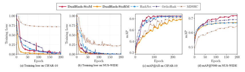
Figure 4: Training loss and the mAP results of DualHash and baselines with 64 bits on CIFAR-10 and NUS-WIDE datasets.

We conduct extensive experiments to evaluate the effectiveness of DualHash against several state-of-the-art hashing methods on three standard image retrieval datasets. All experiments use PyTorch 1.12.1 with CUDA 11.3 on an NVIDIA V100 GPU platform. Visualizations are implemented using Python on macOS 15.3.2.

VI-A Experimental Setup

Datesets. CIFAR-10 is a single-label dataset comprising 60,000 $32\times 32$ color images from 10 classes. In our experiment, we randomly sample 1,000 images per class (10,000 total) for training, 500 per class (5,000 total) for validation, and 500 per class (5,000 total) for testing. NUS-WIDE is a multi-label dataset containing approximately 270,000 web images, each annotated with one or more labels from 81 categories. Following [74, 49, 8]. In our experiment, we use a subset of 195,834 images from the 21 most frequent concepts (each with at least 5,000 images) and randomly sample 700 images per class (14,700 total) for training, 300 per class (6,300 total) for validation, and 300 per class (6,300 total) for testing. ImageNet is a large-scale image dataset from the Large Scale Visual Recognition Challenge (ILSVRC 2015) [32]. It contains over 1.2M images in the training set and 50K images in the validation set, where each image is single-labeled by one of the 1,000 categories. Following [4], in our experiment, we randomly select 100 categories to create ImageNet-100. We use 100 images per category (10,000 total) for training, 30 per category (3,000 total) for validation, and 50 per category (5,000 total) for testing. The training, validation, and testing sets are mutually exclusive with no data overlap.

Training Setup. It is worth noting that our method is compatible with different similarity measurement paradigms, including pointwise, pairwise and tripletwise methods. In our experiments, we focus on deep supervised pairwise hashing using a pairwise cross-entropy loss $f$ and the nonsmooth W-type regularization term $h(z)=\lambda\||\bm{z}|-1\|_{1}$.

Baselines. We compare against eight baselines: SDH [73]; four deep hashing methods with W-type regularizations (DHN [34], DSH [8], DTSH [50], MDSHC [17]); and three state-of-the-art methods addressing quantization error (HashNet [4], DSDH [7], OrthoHash [16]). Following [8], we report the mean Average Precision (mAP), precision curves (AP@topK), and precision within Hamming radius 2 (AP@r=2). Detailed definitions and a full introduction of the baselines are provided in the Supplementary Materials A.

Architecture. For fair comparison, all deep learning-based methods employ AlexNet and ResNet-50 as the backbone network and replace the ReLU activation with ELU to leverage its 1-Lipschitz continuous gradient property for satisfying the smoothness assumption (˜1(ii)). All images are resized to $256\times 256$ pixels and center-cropped to $224\times 224$. We fine-tune the pre-trained convolutional layers (conv1–conv5) and fully connected layers (fc6–fc7), while initializing any newly added layers with Kaiming initialization. For the non-deep method (SDH [73]), we use the following hand-crafted features: 512-dimensional GIST vectors for CIFAR-10, 500-dimensional bag-of-words features for NUS-WIDE, and 1024-dimensional CNN features for ImageNet-100. During training, we monitor validation performance in real-time to observe convergence behavior and adjust hyperparameters accordingly. For evaluation, we use the training set as the retrieval database and the test set as queries.

Hyperparameter Settings. All models are trained for a maximum of 300 epochs with early stopping based on validation mAP. We use a fixed mini-batch size of 256 for CIFAR-10 and 128 for NUS-WIDE and ImageNet-100. For DualHash-StoM, the learning rate $\eta_{k}$ is selected from $\{10^{-4},10^{-3},10^{-2},10^{-1}\}$ with step decay, approximating $\eta_{k}\sim O(L_{F}^{-1})$ without computing $L_{F}$. For DualHash-StoRM, $\eta_{k}$ is chosen from $\{5\times 10^{-3},5\times 10^{-2},5\times 10^{-1}\}$ following $\mathcal{O}(T^{-1/3})$ scaling, and $\rho_{k}$ is selected from $\{0.01,0.05,0.1,0.2,0.7\}$ via cross-validation. All methods use momentum parameters $\alpha^{k}=\beta^{k}=0.905$. The proximal operator for $h^{*}(\cdot)$ requires $\tau<\lambda$ to ensure well-defined updates. We tune $\lambda\in\{10^{-3},10^{-2},10^{-1}\}$ and set $\tau$ accordingly. For all datasets, we set $\tau=10^{-2}$, $\lambda=5\times 10^{-2}$, and $\gamma=3$, with $\lambda$ updated using a step size of $0.1\tau$. All results represent averages over 10 independent runs.

VI-B Convergence Validation

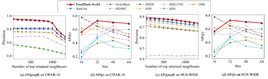
Figure 5: Retrieval performance of DualHash and baselines on CIFAR-10 and NUS-WIDE datasets. (a), (c): AP@topK with 64 bits; (b), (d): AP@r(=2) with different numbers of bits.

TABLE III: The mAP results of DualHash and baselines with different numbers of bits
on CIFAR-10 and NUS-WIDE datasets with ResNet50 backbone.

	CIFAR-10 (mAP@All)				NUS-WIDE (mAP@5000)
Method (ResNet50)	16 bits	32 bits	48 bits	64 bits	16 bits	32 bits	48 bits	64 bits
DSH [8]	0.7403	0.8116	0.8217	0.8239	0.5559	0.6952	0.6981	0.7165
OrthoHash [16]	0.9032	0.9182	0.9202	0.9224	0.7448	0.7600	0.7569	0.7863
MDSHC [17]	0.8980	0.9007	0.9063	0.9227	0.6428	0.7002	0.7248	0.7758
DualHash-StoM	0.8559	0.9202	0.9392	0.9416	0.6538	0.7783	0.7721	0.8016

Bold values indicate the best results.

We validate our theoretical results (Theorems 1 and 2) and compare with HashNet, OrthoHash, and MDSHC with 64 bits on both datasets. Figure˜4 shows the training loss and validation mAP curves over epochs. As shown in Figure˜4 (a)-(b), DualHash-StoRM achieves the fastest convergence and lowest loss values on both datasets, requiring only approximately 25 epochs on CIFAR-10. This aligns with our theoretical outcome: the variance reduction mechanism accelerates convergence. Though slower than DualHash-StoRM, DualHash-StoM still outperforms other baselines (approximately 75 epochs on CIFAR-10). Meanwhile, Figure˜4 (c)-(d) show that although DualHash-StoRM converges faster during training, DualHash-StoM ultimately exhibits superior retrieval performance compared to other baselines.

VI-C Comparison of Retrieval Performance

TABLE IV: The mAP results of DualHash and baselines with different numbers of bits on the ImageNet-100 dataset with ResNet50 backbone.

	ImageNet-100 (mAP@1000)
Method (ResNet50)	16 bits	32 bits	48 bits	64 bits
DSH [8]	0.7179	0.7448	0.7335	0.7585
OrthoHash [16]	0.8040	0.8292	0.8510	0.8636
MDSHC [17]	0.8047	0.8131	0.8561	0.8657
DualHash-StoM	0.7402	0.7705	0.8662	0.8714

Bold values indicate the best results.

We report retrieval performance on CIFAR-10 and NUS-WIDE datasets, as shown in Table II and Figure˜5. In terms of mAP, DualHash methods consistently outperform most baselines, including recent advanced methods like OrthoHash and MDSHC. On CIFAR-10, DualHash-StoM achieves 0.8539 mAP with 64 bits, outperforming OrthoHash (0.8355). On the NUS-WIDE dataset, it reaches 0.7448 mAP, significantly superior to MDSHC (0.6493). Although slightly less accurate than the StoM variant, DualHash-StoRM remains comparable to other baselines, providing a trade-off between accuracy and efficiency.

To further demonstrate the scalability of our approach, we evaluate our method and three baselines using a ResNet50 backbone. As shown in Table˜III, this modern architecture brings substantial performance gains in terms of mAP for all methods across both datasets. Our DualHash-StoM, for example, achieves mAP improvements of 10.3% on CIFAR-10 (0.9416 vs 0.8539) and 9.1% on NUS-WIDE (0.8016 vs 0.7448) at 64 bits. Nevertheless, our method consistently maintains peak performance at 32 bits or more, outperforming all baseline methods. Moreover, on the more complex ImageNet-100 dataset, our method continues to demonstrate superior performance. As reported in Table˜IV, DualHash-StoM reaches 86.62% and 87.14% mAP at 48 and 64 bits, outperforming all baselines. These results confirm that our method maintains robust performance and strong generalization capability as data complexity increases.

For AP@topK (Figure˜5 (a),(c)), DualHash maintains 0.9 precision at lower top-k values on CIFAR-10, significantly outperforming other methods. This indicates that our method is suitable for precision-oriented image retrieval systems. For AP@r metric (Figure˜5 (b),(d)), DualHash-StoM consistently maintains peak performance at 32 bits and above, with 32 bits being optimal across both datasets. These results align with the fact that as bit length increases, the Hamming space becomes sparse and few data points fall within the Hamming ball with radius 2 [75].

VI-D Quantization Error Analysis

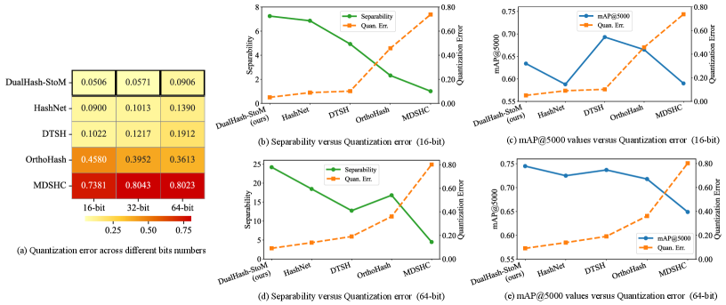
Figure 6: Quantization error and its impact on retrieval performance across different numbers of bits on NUS-WIDE.

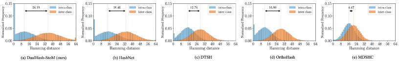
Figure 7: Histogram of intra-class and inter-class Hamming distances of DualHash and baselines with 64 bits on the NUS-WIDE dataset. The arrow annotation is the separability in Hamming distances, $\mathbb{E}[D_{inter}]-\mathbb{E}[D_{intra}]$. We normalized the frequency so that the sum of all bins equals to 1.

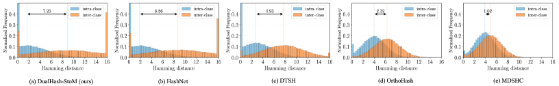
Figure 8: Histogram of intra-class and inter-class Hamming distances of DualHash and baselines with 16 bits on NUS-WIDE.

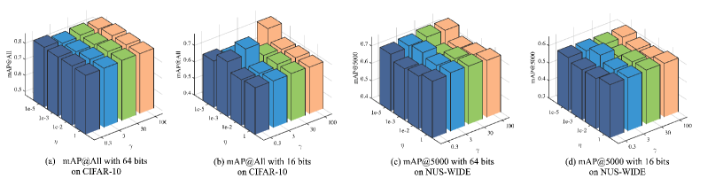
Figure 9: The mAP results of DualHash-StoM with Different settings of $\eta$ and $\lambda$ with 64 & 16 bits on CIFAR-10 and NUS-WIDE.

To elucidate the mechanisms behind the performance of DualHash, following -[16], we examine the quantization error (the discrepancy between continuous outputs and binary codes, Figure˜6) and the Hamming distance distributions of the resulting hash codes (Figures˜7 and 8) across different bit lengths $K$ on the NUS-WIDE dataset. We compare DualHash-StoM against four deep hashing methods: HashNet [4] and OrthoHash [16] (employing distinct quantization strategies), and DTSH [50] and MDSHC [17] (both utilizing $W$-type regularization).

Quantization Error Correlates with Intra- and Inter-class Distances. We find that methods achieving smaller quantization errors produce hash codes with reduced intra-class distances and enhanced inter-class separability, as shown in Figure˜6(a) and Figures˜8 and 7. In the 64-bit setting (Figure˜7), both HashNet and DualHash exhibit similar inter-class distributions (close to Hamming distance $K/2=32$). However, DualHash’s lower quantization error (0.0906 vs. 0.1390) enables significantly superior separability, i.e., the difference in the mean of intra-class distance (the blue dotted line) with the mean of inter-class distance (the orange dotted line). In contrast, MDSHC’s high quantization error (0.8023) leads to substantially larger intra-class distances and weaker inter-class separation, yielding a $5\times$ inferior separability ratio (24.19 vs. 4.47). This demonstrates that reducing quantization error enhances code quality primarily by compressing intra-class distributions.

DualHash Achieves Lower Quantization Error via Dual-Space Reformulation. As shown in Figure˜6(a), DualHash attains the smallest quantization error across different bit lengths among all evaluated methods. This performance advantage stems from a fundamental methodological innovation: DualHash employs a novel dual-space reformulation of the W-regularization. The convexity property inherent in our dual formulation’s conjugate function yields significant optimization advantages compared to directly optimizing the original nonconvex regularization or activation functions.

Bit-Dependent Performance and the Separability-Semantics Trade-off. While lower quantization error generally improves separability (Figure˜6(b) and (d)), its impact on retrieval performance varies significantly across bit settings, revealing a fundamental trade-off between class separability and semantic preservation.

High-bit regime ($K=64$): Lower quantization error helps produce high mAP. At $K=64$ (Figures 6(d) and (e)), lower quantization error consistently correlates with higher mAP by enhancing separability and preserving both semantic discriminability and visual feature quality. Methods achieving low quantization loss (e.g., DualHash, HashNet, and DTSH) demonstrate superior retrieval accuracy, with DualHash achieving peak mAP performance.

Low-bit regime ($K=16$): Low quantization error may produce low performance. At $K=16$ (Figure˜6(b) and (c)), we observe a contrasting pattern: both extremely low and extremely high quantization error methods yield suboptimal performance. Notably, DTSH, which maintains intermediate quantization error, achieves superior mAP. Methods with very low quantization error (e.g., DualHash and HashNet) exhibit relatively lower mAP, particularly on multi-label datasets (e.g., NUS-WIDE). Specifically, we observe that DualHash generates hash codes with low intra-class distances and high inter-class separation. This creates relatively clean class separation, but the actual visual relationships between images may get lost. Consequently, DualHash excels on simple datasets like CIFAR-10 but shows relatively lower performance on complex multi-label datasets like NUS-WIDE and ImageNet-100.

VI-E Parameter Sensitivity Analysis

To explore the sensitivity of key hyperparameters $\lambda$ and $\gamma$ in DualHash, we conduct a grid search with $\lambda\in\{10^{-5},10^{-3},10^{-2},1\}$ and $\gamma\in\{0.3,3,30,100\}$. Unlike many deep hashing methods that exhibit significant hyperparameter sensitivity, DualHash-StoM demonstrates robust performance across a wide range of hyperparameter combinations (see Figure˜9). Specifically, 64-bit codes achieve excellent stability with mAP variations below 3% on CIFAR-10 and 8% on NUS-WIDE. While 16-bit codes show greater sensitivity (up to 18% on CIFAR-10), this behavior is consistent with the intrinsic optimization challenges of extremely compact hash codes. Overall, the method demonstrates strong stability for standard hash lengths ($\geq$64 bits), which simplifies hyperparameter tuning in practical high-precision retrieval applications.

VII Conclusion and Discussion

This paper proposed DualHash, a stochastic primal-dual algorithm for deep hashing with rigorous non-asymptotic convergence guarantees. Our approach effectively addressed the fundamental optimization challenge of W-type regularization with nonlinear composition through a novel “decoupling-dual-structure” strategy: transforming the nonconvex regularizer into a convex dual space with closed-form proximal updates. We provided a distinct theoretical framework beyond conventional primal-dual analysis, establishing complexity bounds of $\mathcal{O}(\varepsilon^{-4})$ for DualHash-StoM and optimal $\mathcal{O}(\varepsilon^{-3})$ for DualHash-StoRM. Extensive experiments validated DualHash achieved superior retrieval performance across all metrics, including the highest mAP at 32 bits or more, consistently lower quantization errors, and stronger robustness on both datasets.

Beyond deep hashing, our core decoupling-dual-structure optimization principle offered a promising pathway for tackling nonconvex regularization challenges in related domains, including neural network quantization [76, 77, 78] and sparse regularized neural network training [79, 80, 81, 10].

Supplementary Material A

This supplementary material provides detailed experimental settings and additional results.

S.I Experiments details

S.I.A Deep Pairwise Supervised Hashing Formulation

TABLE V: Summary of symbols and notations.

Symbol	Description
$\bm{a}_{i}$, $\bm{y}_{i}$	Input feature and label vector for
	$i$-th sample
$s_{ij}^{o}$, $s_{ij}^{h}$	Similarity in input space and
	Hamming space
$d_{ij}^{o}$, $d_{ij}^{h}$	Distance in input space and
	Hamming space
$\bm{C}(\bm{x};\bm{a}_{i})$	Network output before activation
$\bm{b}_{i}\in\{-1,1\}^{d}$	Binary hash code for $i$-th sample
$\bm{u}_{i}=\tanh(\bm{C}(\bm{x};\bm{a}_{i}))$	Continuous code after activation
$n$, $d$	Number of samples and hash
	code length
$\bm{x}$	Network parameters
$d_{\bm{a}}$, $d_{x}$	Dimension of input feature and
	parameters

We consider deep supervised pairwise hashing in our experiments, which aims to learn binary codes that minimize Hamming distances for similar pairs and maximize them for dissimilar pairs. Let $\bm{A}=\{\bm{a}_{i}\in\mathbb{R}^{d_{a}}:i=1,\ldots,n\}$ be the training set with labels $\mathcal{Y}=\{\bm{y}_{i}\in\{0,1\}^{C}\}$ (one-hot for single-label, multi-hot for multi-label). Key notations are in Table˜V.

Network Architecture. A CNN extracts features from $\bm{a}_{i}$, followed by a fully connected hash layer producing $d$-dimensional outputs $\bm{C}(\bm{x};\bm{a}_{i})$, which are passed through $\tanh$ to yield $\bm{u}_{i}$.

Loss Function. For hash codes in $\{-1,1\}^{d}$, the Hamming distance is $d_{ij}^{h}=\tfrac{1}{2}(d-\langle\bm{h}_{i},\bm{h}_{j}\rangle)$. Following [3, 49], similarity $s^{o}_{ij}=1$ if samples share labels, else $0$. The likelihood is:

$$P(s^{o}_{ij}\mid\bm{h}_{i},\bm{h}_{j})=\sigma(\langle\bm{h}_{i},\bm{h}_{j}\rangle)^{s^{o}_{ij}}\left(1-\sigma(\langle\bm{h}_{i},\bm{h}_{j}\rangle)\right)^{1-s^{o}_{ij}},$$

where $\sigma(x)=(1+\exp(-\alpha x))^{-1}$, $\alpha<1$. Using continuous codes $\bm{u}_{i}$ and $s^{h}_{ij}=\tfrac{1}{2}\langle\bm{u}_{i},\bm{u}_{j}\rangle$, the loss becomes:

$$\min_{\bm{x}}\;\mathcal{L}_{S}(\bm{x})=-\frac{1}{|\mathcal{S}|}\sum_{s^{o}_{ij}\in\mathcal{S}}\log\left(1+\exp\left(-\alpha s^{o}_{ij}s^{h}_{ij}\right)\right).$$ (S1)

We use the W-type regularization:

$$h(\bm{Z})=\sum_{i=1}^{n}h(\bm{z}_{i}),\quad h(\bm{z})=\lambda\|\,|\bm{z}|-\bm{1}\,\|_{1},$$ (S2)

where $\lambda>0$ controls regularization strength.

Combining (S1) and (S2) into (III-B) gives the final loss of DualHash in our experiments.

$$\min_{\bm{x}\in\mathcal{X},\bm{B}\in\mathcal{B}}\; -\frac{1}{|\mathcal{S}|}\sum_{s^{o}_{ij}\in\mathcal{S}}\log\left(1+\exp\left(-\alpha s^{o}_{ij}s^{h}_{ij}\right)\right)$$

$$+\frac{\gamma}{2n}\sum_{i=1}^{n}\|\bm{b}_{i}-\bm{u}_{i}\|_{2}^{2}+\sum_{i=1}^{n}\lambda\|\,|\bm{b}_{i}|-\bm{1}\,\|_{1}.$$ (S3)

Out-of-sample Extension. For an unseen query $\bm{a}_{q}\notin\bm{A}$, its binary code is predicted as:

$$\bm{b}_{q}=\operatorname{sgn}(\bm{C}(\bm{x};\bm{a}_{q})).$$

S.I.B Details of experiment implementation

Baseline methods We compare our method with eight baseline approaches, including one traditional discrete hashing method and seven deep supervised hashing methods:

1. SDH [73]: A pointwise supervised hashing method using hand-crafted features. It employs discrete cyclic coordinate descent to directly optimize binary codes.

2. DHN [34]: A Bayesian framework that minimizes pairwise cross-entropy loss and quantization error using $\tanh$ relaxation and $\sum_{i}\log(\cosh(|z_{i}|-1))$ regularization.

3. DSH [8]: Uses max-min pairwise loss with $\||\bm{z}|-\bm{1}\|_{1}$ regularization to minimize quantization error.

4. DTSH [50]: Learns hash codes by maximizing triplet likelihood with negative log-triplet loss, using $\||\bm{z}|-\bm{1}\|^{2}_{2}$ quantization regularization and a positive margin $\alpha$ to accelerate training and normalize Hamming distance gaps.

5. HashNet [4]: Progressively increases $\beta$ in $\tanh(\beta x)$ to approximate the sgn function, addressing nonconvex optimization challenges.

6. DSDH [7]: Integrates pairwise labels and classification information using alternating minimization to learn features and binary codes with the sgn function.

7. OrthoHash [16]: Uses a single cosine similarity loss to maximize alignment between continuous codes and binary orthogonal codes, ensuring discriminativeness with minimal quantization error.

8. MDSHC [17]: A two-stage method that first generates hash centers with minimal Hamming distance constraints, then uses three-part losses with $\||\bm{z}|-\bm{1}\|_{1}$ regularization to reduce quantization error.

Evaluation Protocols Following [8], we adopt three evaluation metrics:

1. Mean Average Precision (mAP): For a query $\bm{x}_{q}$, the Average Precision is computed as:

   $$\text{AP}(\bm{x}_{q})=\frac{\sum_{k=1}^{N}P(k)\cdot\mathbb{I}_{\text{rel}}(k)}{\min(N,R_{q})},$$

   where $P(k)$ is precision at rank $k$, $\mathbb{I}_{\text{rel}}(k)$ indicates whether the $k$-th result is relevant, $R_{q}$ is the total relevant samples, and $N$ is the number of retrieved items. mAP averages AP over all queries. For CIFAR-10, we use all returned neighbors; for NUS-WIDE, we consider top-5000 results.

2. Precision at Top K (AP@topK): The proportion of true neighbors among top-K retrieved results, averaged over all queries.

3. Precision within Hamming Radius 2 (AP@r): Measures retrieval accuracy for items within Hamming distance 2 from the query. This metric is particularly efficient as Hamming radius search has $\mathcal{O}(1)$ time complexity per query.

4. Precision-recall curves of Hamming ranking: PR curves illustrate precision at various levels of recall, offering insights into the trade-off between precision and recall at different thresholds. These curves are widely recognized as effective indicators of the robustness and overall performance of different algorithms.

S.II Additional Experiments

S.II.A Comparison of Optimization Algorithms with Different W-Type Regularizations

TABLE VI: Configurations of different W-type regularizations and optimization algorithms
for DualHash-StoM and three baselines.

Method	$h(\bm{z})$	Convexity	Algorithm	Complexity
DSH [8]	$\||\bm{z}|-\mathbf{1}\|_{1}$	Nonconvex	SGDM	–
StoMHash-WCR	$\|\bm{z}^{2}-\mathbf{1}\|_{1}$	Weakly convex	SPGD	–
DHN [34]	$\sum_{i}\log(\cosh(|z_{i}|-1))$	Nonconvex	SGDM	–
DualHash-StoM	$\||\bm{z}|-\mathbf{1}\|_{1}$	Nonconvex	PD	$\checkmark$

Notes: Algorithm describes the optimization strategy: SGDM (stochastic subgradient descent with momentum), SPGD (stochastic proximal gradient descent), PD (primal-dual). Complexity reports oracle complexity; ‘–’ indicates no analysis available.

To validate the effectiveness of our primal-dual framework, we compare DualHash-StoM against optimization algorithms with different W-type regularizations. Table˜VI summarizes the configurations of different regularization functions and their corresponding optimization approaches. For StoMHash-WCR, we employ the regularization $\lambda\|\bm{z}^{2}-\mathbf{1}\|_{1}$ following the iSPALM framework [82]. The proximal operator is computed with parameter $\rho>0$ under the condition $\frac{\rho}{\eta}>\frac{1}{2}$, which ensures the subproblem is strongly convex with a unique solution.

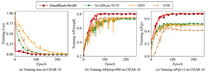
Figure 10: Training performance comparison of DualHash-StoM and three baselines with 64 bits on the CIFAR-10 dataset.

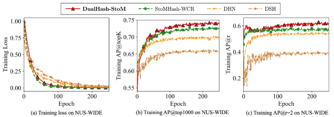
Figure 11: Training performance comparison of DualHash-StoM and three baselines with 64 bits on the NUS-WIDE dataset.

Training performance analysis

TABLE VII: Retrieval performance comparison of DualHash-StoM and three baselines with 64 bits
on CIFAR-10 and NUS-WIDE datasets

Methods	CIFAR-10			NUS-WIDE
	mAP@All	AP@r	Time*	mAP@5000	AP@r	Time*
DSH [8]	0.8010	0.4401	7.38	0.6634	0.4004	21.14
DHN [34]	0.8051	0.5272	6.74	0.7042	0.5432	16.47
StoMHash-WCR	0.7773	0.5402	7.04	0.7225	0.5857	16.69
DualHash-StoM	0.8539	0.6872	6.86	0.7448	0.6548	16.83

^*Training time per epoch (seconds). Red and blue indicate highest and second highest values.

Figures 10 and 11 present training dynamics across different optimization approaches, comparing training loss, AP@top1000, and AP@r=2 metrics with 64 bits on both datasets. On CIFAR-10, DualHash-StoM demonstrates superior optimization efficiency across all metrics. Our method achieves the fastest convergence in training loss while consistently maintaining the highest AP@r and AP@top1000 values throughout the optimization process. While StoMHash with weakly convex regularization (StoMHash-WCR) shows competitive performance, DualHash-StoM achieves both faster convergence and consistently higher performance, demonstrating the effectiveness of our primal-dual transformation for handling W-type regularizations. On the more challenging NUS-WIDE dataset with complex multi-label scenarios, DualHash-StoM maintains competitive retrieval performance despite slightly slower initial convergence. The experimental results on diverse datasets confirm our core motivation: utilizing nonconvex nonsmooth regularization with specialized primal-dual optimization significantly improves hash code learning and retrieval performance in practical applications.

Retrieval performance in hamming space We report mAP, AP@r, and the average time per training epoch on both datasets, all with 64-bit codes, for different methods in Table VII. The results highlight the superior retrieval accuracy of DualHash-StoM compared to the baseline methods.

Specifically, on the CIFAR-10 dataset, DualHash-StoM achieves 9.9% and 27.2% improvements over StoMHash-WCR in mAP@All and AP@r, respectively. Similarly, on the NUS-WIDE dataset, DualHash-StoM outperforms StoMHash-WCR with a 3.1% improvement in mAP@5000 and an 11.8% improvement in AP@r. Computationally, DualHash-StoM shows comparable efficiency to baselines such as DHN (e.g., 6.86s vs. 6.74s on CIFAR-10 and 16.83s vs. 16.47s on NUS-WIDE). This marginal time increase is justified by the substantial performance gains.

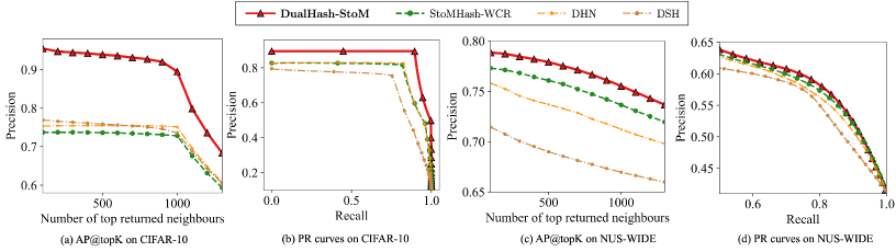
Figure 12: Retrieval performance comparison of DualHash-StoM and three baselines with 64 bits on CIFAR-10 and NUS-WIDE datasets. (a), (c): AP@topK results; (b), (d): PR curves.

Furthermore, Figure˜12 displays AP@topK results and PR curves with 64-bit codes on both datasets. DualHash-StoM consistently outperforms all comparison methods by large margins in AP@topK. For PR curves, DualHash-StoM demonstrates superior performance at lower recall levels, making it especially well-suited for precision-critical image retrieval systems.

Supplementary Material B

This supplementary material provides useful definitions and propositions, necessary lemmas with detailed proofs, and the complete derivations for the main theoretical results and parameters presented in the primary work.

S.III Preliminaries

The proximal mapping admits the following properties.

Proposition 1 (Properties of proximal operators [54])

Let $f:\mathbb{R}^{q}\rightarrow\mathbb{R}\cup\{+\infty\}$ be proper and closed. Then, the following holds.

1. The set $\operatorname{prox}_{\tau f}(\bm{x})$ is nonempty and compact for any $\bm{x}\in\mathbb{R}^{q}$ and $\tau>0$.

2. If $f$ is convex, then $\operatorname{prox}_{\tau f}(\bm{x})$ contains exactly one value for any $\bm{x}\in\mathbb{R}^{q}$ and $\tau>0$.

We introduce the following definitions related to subdifferentials.

Definition 1 (Subdifferentials [54])

Let $f:\mathbb{R}^{q}\to(-\infty,+\infty]$ be a proper closed function.

1. For a given $\bm{x}\in\operatorname{dom}f$, the Fréchet subdifferential, or simply of $f$ at $\bm{x}$, written $\hat{\partial}f(\bm{x})$, is the set of all vectors $\bm{u}\in\mathbb{R}^{q}$ that satisfy

   $$\liminf_{\bm{y}\neq\bm{x},\bm{y}\to\bm{x}}\frac{f(\bm{y})-f(\bm{x})-\langle\bm{u},\bm{y}-\bm{x}\rangle}{\|\bm{y}-\bm{x}\|}\geq 0.$$

2. The limiting-subdifferential, or simply the subdifferential, of $f$ at $\bm{x}$, written $\partial f(\bm{x})$, is defined through the following closure process

   $$\partial f(\bm{x}):=\{\bm{u}\in\mathbb{R}^{q}:\exists\bm{x}^{k}\to\bm{x},f(\bm{x}^{k})\to f(\bm{x}),\bm{u}^{k}\in\hat{\partial}f(\bm{x}^{k})\to\bm{u}\text{ as }k\to\infty\}.$$

Notionally, $\hat{\partial}f(\bm{x})=\partial f(\bm{x})=\emptyset$ for all $\bm{x}\notin\operatorname{dom}(f)$. From definition definition˜1 it follows that $\hat{\partial}f(\bm{x})\subset\partial f(\bm{x})$ for all $\bm{x}\in\operatorname{dom}(f)$. Moreover, $\hat{\partial}f(\bm{x})$ is closed convex while $\partial f(\bm{x})$ is merely closed. In particular, if $f$ is convex, then

$$\hat{\partial}f(\bm{x})=\partial f(\bm{x})=\{\bm{d}\in\mathbb{R}^{q}\mid f(\bm{y})\geq f(x)+\langle\bm{d},\bm{y}-\bm{x}\rangle,\,\forall\bm{y}\in\mathbb{R}^{q}\}.$$

The following proposition lists several useful properties of subgradients.

Proposition 2 (Properties of subdifferential [62])

Let $f:\mathbb{R}^{q_{1}}\rightarrow(-\infty,\infty]$ and $g:\mathbb{R}^{q_{2}}\rightarrow(-\infty,\infty]$ be proper and lower semicontinuous, and let $h:\mathbb{R}^{q_{1}}\rightarrow\mathbb{R}$ be continuously differentiable. Then the following results hold:

1. For any $\bm{x}\in\mathbb{R}^{q_{1}}$, we have $\hat{\partial}f(\bm{x})\subseteq\partial f(\bm{x})$. If, in addition, $f$ is convex, we have $\hat{\partial}f(\bm{x})=\partial f(\bm{x})$.

2. For $\bm{x}\in\mathbb{R}^{q_{1}}$ with $f(\bm{x})<\infty$, it holds

   $$\hat{\partial}(f+h)(\bm{x}) =\hat{\partial}f(\bm{x})+\nabla h(\bm{x})\quad\text{and}$$

   $$\partial(f+h)(\bm{x}) =\partial f(\bm{x})+\nabla h(\bm{x}).$$

3. If $\sigma(\bm{x}_{1},\bm{x}_{2})=f_{1}(\bm{x}_{1})+f_{2}(\bm{x}_{2})$, then

   $$\begin{pmatrix}\hat{\partial}_{\bm{x}_{1}}f_{1}(\bar{\bm{x}}_{1})\\ \hat{\partial}_{\bm{x}_{2}}f_{2}(\bar{\bm{x}}_{2})\end{pmatrix}\subseteq\hat{\partial}\sigma(\bar{\bm{x}}_{1},\bar{\bm{x}}_{2})\quad\text{and}\quad\begin{pmatrix}\partial_{\bm{x}_{1}}f_{1}(\bar{\bm{x}}_{1})\\ \partial_{\bm{x}_{2}}f_{2}(\bar{\bm{x}}_{2})\end{pmatrix}\subseteq\partial\sigma(\bar{\bm{x}}_{1},\bar{\bm{x}}_{2}).$$

For Algorithm˜1, we establish key relationships among iterates via the momentum acceleration framework in (IV.6).

Proposition 3 (Lemma 5.2 in [82])

Let $\{\bm{x}^{k}\}_{k\in\mathbb{N}}$, $\{\bm{y}^{k}\}_{k\in\mathbb{N}}$, and $\{\bm{z}^{k}\}_{k\in\mathbb{N}}$ be sequences generated by (IV.6). For all $k\in\mathbb{N}$, we have:

1. $\|\bm{x}^{k}-\bm{y}^{k}\|^{2}=\alpha_{k}^{2}\|\bm{x}^{k}-\bm{x}^{k-1}\|^{2}$,

2. $\|\bm{x}^{k}-\bm{z}^{k}\|^{2}=\beta_{k}^{2}\|\bm{x}^{k}-\bm{x}^{k-1}\|^{2}$,

3. $\|\bm{x}^{k+1}-\bm{y}^{k}\|^{2}\geq 2(1-\alpha_{k})\|\bm{x}^{k+1}-\bm{x}^{k}\|^{2}+2\alpha_{k}(\alpha_{k}-1)\|\bm{x}^{k}-\bm{x}^{k-1}\|^{2}$.

For Algorithm˜2, we employ the STORM (STochastic Recursive Momentum) variance reduction estimator [63]. In stochastic optimization problems where $F(\bm{x})=\mathbb{E}_{\xi}[F(\bm{x};\xi)]$ with $\xi\in\Xi$, standard momentum methods use

$$\bm{d}^{k}=\rho_{k}\nabla F(\bm{x}^{k},\xi^{k})+(1-\rho_{k})\bm{d}^{k-1},\text{ where }\rho_{k}\in[0,1],$$

yielding a biased estimate of $\nabla F(\bm{x}^{k})$. STORM adds a correction term, $(1-\rho_{k})(\nabla F(\bm{x}^{k},\xi^{k})-\nabla F(\bm{x}^{k-1},\xi^{k})$, resulting in:

$$\bm{d}^{k}=\left\{\begin{array}[]{ll}\nabla F\left(\bm{x}^{k},\xi^{k}\right),&\text{if }k=1,\\ \nabla F\left(\bm{x}^{k},\xi^{k}\right)+\left(1-\rho_{k}\right)\left(\bm{d}^{k-1}-\nabla F\left(\bm{x}^{k-1},\xi^{k}\right)\right),&\text{if }k>1,\end{array}\right.$$

$$\bm{x}^{k+1}=\bm{x}^{k}-\eta_{k}\bm{d}^{k}.$$

This exploits the smoothness of $F(\cdot,\xi)$, leading to efficient variance reduction. When $\rho_{k}=1$, $\bm{d}^{k}$ reduces to vanilla mini-batch SGD. We set $\rho_{k}\in(0,1)$ for $k\geq 1$ in Algorithm˜2.

S.IV Discussions on ˜1(ii) in Section˜V

This section verifies that the smoothness constant $L_{F}$ in ˜1(ii) is independent of the sample size $n$, which is essential for our convergence analysis.

For the smooth properties of mappings in our problem, we consider the nonlinear mapping $\mathcal{D}(\bm{x})=(\bm{D}_{1}(\bm{x}),\ldots,\bm{D}_{n}(\bm{x}))$ from $\mathcal{X}\subseteq\mathbb{R}^{d_{\bm{x}}}$ to $\mathbb{R}^{n\times d}$, and make the following assumption:

Assumption 3 (Properties of $\mathcal{D}$)

Suppose there exist constants $L_{\mathcal{D}},\,L_{\nabla\mathcal{D}}>0$ such that for any $\bm{x},\bm{x}^{\prime}\in\mathcal{X}$: $\|\mathcal{D}(\bm{x})-\mathcal{D}(\bm{x}^{\prime})\|\leq L_{\mathcal{D}}\|\bm{x}-\bm{x}^{\prime}\|$ and $\|\nabla\mathcal{D}(\bm{x})-\nabla\mathcal{D}(\bm{x}^{\prime})\|\leq L_{\nabla\mathcal{D}}\|\bm{x}-\bm{x}^{\prime}\|$.

Combining ˜1(i) and ˜3, we can establish that there exist constants $C_{\mathcal{D}},G_{\mathcal{D}},C_{\mathcal{D}\mathcal{B}}>0$ such that:

$$\|\mathcal{D}(\bm{x})\|\leq C_{\mathcal{D}},\,\|\nabla\mathcal{D}(\bm{x})\|\leq G_{\mathcal{D}},\,\text{and}\quad\|\mathcal{D}(\bm{x})-\bm{B}\|\leq C_{\mathcal{D}\mathcal{B}}.$$

Based on these assumptions, we can establish the smoothness properties of the composite function $F$. First, we observe that $P(\bm{x},\bm{B})$ is $\frac{\gamma}{n}$-smooth with respect to $\bm{B}$ and $\frac{\gamma}{n}(L_{\nabla\mathcal{D}}(C_{\mathcal{D}}+C_{\bm{B}})+G_{\mathcal{D}}L_{\mathcal{D}})$-smooth with respect to $\bm{x}$. Combining these properties, $P(\bm{x},\bm{B})$ has an overall smoothness constant:

$$L_{s}=\frac{\gamma}{n}\sqrt{2\max\{L^{2}_{\nabla\mathcal{D}}C^{2}_{\mathcal{D}\mathcal{B}}+(2G_{\mathcal{D}}^{2}+1)L^{2}_{\mathcal{D}},2G_{\mathcal{D}}^{2}+1\}}=\mathcal{O}(1)$$

Consequently, $F(\bm{x},\bm{B})$ is $L_{F}$-smooth with respect to $(\bm{x},\bm{B})$, where $L_{F}=\mathcal{O}(1)$. An important observation is that, despite $C_{\mathcal{D}}$, $G_{\mathcal{D}}$ and $C_{\mathcal{D}\mathcal{B}}$ potentially being $\mathcal{O}(\sqrt{n})$, the overall smoothness constant $L_{F}$ remains independent of the sample size $n$, which is crucial for our convergence analysis. This smoothness property implies the following descent lemma for $F$ with respect to $\bm{x}$ and $\bm{B}$:

$$F(\bm{x}^{\prime},\bm{B})\leq F(\bm{x},\bm{B})+\langle\nabla_{\bm{x}}F(\bm{x},\bm{B}),\bm{x}^{\prime}-\bm{x}\rangle+\frac{L_{F}}{2}\|\bm{x}-\bm{x}^{\prime}\|^{2}$$ (S1)

for any $\bm{B}\in\mathcal{B}$; and similarly for $\bm{B}$:

$$F(\bm{x},\bm{B}^{\prime})\leq F(\bm{x},\bm{B})+\langle\nabla_{\bm{B}}F(\bm{x},\bm{B}),\bm{B}^{\prime}-\bm{B}\rangle+\frac{L_{F}}{2}\|\bm{B}-\bm{B}^{\prime}\|^{2}$$ (S2)

for any $\bm{x}\in\mathcal{X}$.

S.V Proofs of the main theorems in Section˜V

Before proceeding, we define the following quantities for notational simplicity:

$$\Delta_{\bm{x}}^{k}=\frac{\|\bm{x}^{k}-\bm{x}^{k-1}\|^{2}}{2},\quad\Delta_{\bm{B}}^{k}=\frac{\|\bm{B}^{k}-\bm{B}^{k-1}\|^{2}_{F}}{2}.$$

We first analyze how the Lagrangian function ($\mathcal{L}$) changes during the updates of primal and dual variables in one iteration. The total change can be decomposed as:

$$\mathcal{L}(\bm{x}^{k+1},\bm{B}^{k+1},\bm{\Lambda}^{k+1})-\mathcal{L}(\bm{x}^{k},\bm{B}^{k},\bm{\Lambda}^{k})$$

$$= \,\underbrace{\mathcal{L}(\bm{x}^{k+1},\bm{B}^{k+1},\bm{\Lambda}^{k+1})-\mathcal{L}(\bm{x}^{k+1},\bm{B}^{k},\bm{\Lambda}^{k})}_{\text{one-iteration progress on $\bm{B}$ and $\bm{\Lambda}$}}+\underbrace{\mathcal{L}(\bm{x}^{k+1},\bm{B}^{k},\bm{\Lambda}^{k})-\mathcal{L}(\bm{x}^{k},\bm{B}^{k},\bm{\Lambda}^{k})}_{\text{one-iteration progress on $\bm{x}$}}.$$ (S1)

S.V.A Common intermediate result

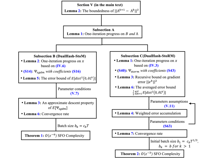
Figure 13: Theoretical analysis framework of DualHash.

Lemma 1 (One-iteration progress on $\bm{B}$ and $\bm{\Lambda}$)

Consider the sequence $\{\bm{x}^{k},\bm{B}^{k},\bm{\Lambda}^{k}\}_{k\in\mathbb{N}}$ generated by Algorithm˜1 or Algorithm˜2. Under ˜1 (ii), for $\forall$ $k\geq 1$, it holds that

$$\mathcal{L}(\bm{x}^{k+1},\bm{B}^{k+1},\bm{\Lambda}^{k+1})-\mathcal{L}(\bm{x}^{k+1},\bm{B}^{k},\bm{\Lambda}^{k})$$

$$\leq \,\underbrace{3\delta\tau^{-1}}_{K_{1}}\Delta_{\bm{B}}^{k+2}-\underbrace{\left(2\tau^{-1}-L_{F}-3\delta\tau(\tau^{-1}+L_{F})^{2}\right)}_{K_{2}}\Delta_{\bm{B}}^{k+1}+\underbrace{\frac{\tau L_{F}^{2}}{\delta}}_{K_{3}}\Delta_{\bm{B}}^{k}+\underbrace{3\delta\tau L_{F}^{2}}_{K_{4}}\Delta_{\bm{x}}^{k+2}+\underbrace{\frac{\tau L_{F}^{2}}{\delta}}_{K_{3}}\Delta_{\bm{x}}^{k+1}$$ (S2)

Proof 1

Using the smoothness of $F$ with respect to $\bm{B}$ in (S2), we conclude that

$$\mathcal{L}(\bm{x}^{k+1},\bm{B}^{k+1},\bm{\Lambda}^{k+1})-\mathcal{L}(\bm{x}^{k+1},\bm{B}^{k},\bm{\Lambda}^{k})$$

$$\leq -\left(\tau^{-1}-\frac{L_{F}}{2}\right)\|\bm{B}^{k+1}-\bm{B}^{k}\|^{2}+\Big\langle\bm{\Lambda}^{k+1}-\bm{\Lambda}^{k},\tau\Big(\nabla_{\bm{B}}F(\bm{x}^{k},\bm{B}^{k-1})-\nabla_{\bm{B}}F(\bm{x}^{k+1},\bm{B}^{k})\Big)\Big\rangle.$$ (S3)

For the inner product term in (1), we apply the block-wise separability of ($\mathcal{L}$) with respect to $\bm{B}=\{b_{i}\}_{i=1}^{n}$ and $\bm{\Lambda}=\{\lambda_{i}\}_{i=1}^{n}$ and obtain

$$\langle\bm{\Lambda}^{k+1}-\bm{\Lambda}^{k},\tau(\nabla_{\bm{B}}F(\bm{x}^{k},\bm{B}^{k-1})-\nabla_{\bm{B}}F(\bm{x}^{k+1},\bm{B}^{k}))\rangle$$

$$\leq \,\frac{\delta\tau}{2}\|\bm{\Lambda}^{k+1}-\bm{\Lambda}^{k}\|^{2}+\frac{\tau}{2\delta}\|\nabla_{\bm{B}}F(\bm{x}^{k+1},\bm{B}^{k})-\nabla_{\bm{B}}F(\bm{x}^{k},\bm{B}^{k+1})\|^{2}$$

$$\leq \,\frac{\delta\tau}{2}\|\bm{\Lambda}^{k+1}-\bm{\Lambda}^{k}\|^{2}+\frac{\delta\tau L_{F}^{2}}{2}\left(\|\bm{x}^{k+1}-\bm{x}^{k}\|^{2}+\|\bm{B}^{k}-\bm{B}^{k-1}\|^{2}\right).$$ (S4)

where the first inequality follows from the fact that $\left<\bm{a},\bm{b}\right>\leq\frac{\delta}{2}\|\bm{a}\|^{2}+\frac{1}{2\delta}\|\bm{b}\|^{2}$ for some $\delta>0$ and the second inequality follows from (S2) agian.

Then, substituting (1) and (V.6) into (1) and rearranging the inequality yield (1). $\square$

We present complexity analyses of two algorithms. Before presenting the results, we introduce the notation that will be used throughout our analysis:

$$\bm{\xi}^{k} =\{\xi_{j}^{k},j\in\mathcal{J}_{k}\}, k$$ (mini-batch at iteration )

$$\bm{\xi}^{[k]} =\{\bm{\xi}^{1},\bm{\xi}^{2},\ldots,\bm{\xi}^{k}\}, k$$ (history of mini-batches up to iteration )

$$\mathbb{E}_{\bm{\xi}^{[k]}}[\cdot] =\mathbb{E}[\cdot|\bm{\xi}^{[k]}].$$ (conditional expectation given history)

For $\bm{d}^{k}\in\partial\mathcal{L}(\bm{x}^{k},\bm{B}^{k},\bm{\Lambda}^{k})$, let us denote $\bm{d}^{k}=(\bm{d}_{\bm{x}}^{k},\bm{d}_{\bm{B}}^{k},\bm{d}_{\bm{\Lambda}}^{k})$ and

$$\begin{cases}&\bm{d}_{\bm{x}}^{k}=\nabla_{\bm{x}}F(\bm{x}^{k},\bm{B}^{k}),\\ &\bm{d}_{\bm{B}}^{k}=\nabla_{\bm{B}}F(\bm{x}^{k},\bm{B}^{k})+\bm{\Lambda}^{k},\\ &\bm{d}_{\bm{\Lambda}}^{k}=\bm{B}^{k}-\mathcal{G}_{\bm{\Lambda}}^{k},\end{cases}$$ (S5)

where $\mathcal{G}_{\bm{\Lambda}}^{k}\in\partial h^{*}(\bm{\Lambda}^{k})$.

Since the updates of $\bm{B}$ and $\bm{\Lambda}$ are common in both Algorithm˜1 and Algorithm˜2, we analyze their effects in Section˜S.V.A. Then, for each algorithm, we separately analyze the change in the Lagrangian function due to the specific update rule for $\bm{x}$. The theoretical analysis framework for both DualHash instances is summarized in Figure˜13.

S.V.B Complexity analysis of DualHash-StoM (Algorithm˜1)

Let us define the gradient error in the $k$-th iteration

$$\bm{e}^{k}=\bm{G}^{k}-\nabla_{\bm{x}}F(\bm{z}^{k},\bm{B}^{k}),$$ (S6)

where $\bm{G}^{k}$ is defined in (IV.5). It is straightforward to estimate the error under ˜1 (iii) as follows: for $\forall\,k\geq 1$,

$$\mathbb{E}_{\bm{\xi}^{[k]}}\left[\|\bm{e}^{k}\|^{2}\right]\leq\frac{\sigma^{2}}{b_{k}}.$$ (S7)

S.V.B1 Main lemmas

Now, we analyze how the Lagrangian function ($\mathcal{L}$) changes during the update of $\bm{x}$ (IV.6). We first present a lemma concerning a property of a continuously differentiable function with a Lipschitz continuous gradient, followed by a proposition that details the interrelations among the sequences $\{\bm{x}^{k}\}_{k\in\mathbb{N}},\,\{\bm{y}^{k}\}_{k\in\mathbb{N}},\,\{\bm{z}^{k}\}_{k\in\mathbb{N}}$ generated by the algorithm.

Lemma 1

Let $f(\bm{x}):\mathbb{R}^{q}\rightarrow\mathbb{R}$ be a continuously differentiable function with $L$-lipschitz continuous gradient. Then, for any $\bm{x},\,\bm{y},\,\bm{z}\in\mathbb{R}^{q}$ and any $\bm{x}^{+}\in\mathbb{R}^{q}$ defined by

$$\bm{x}^{+}=\bm{y}-\eta\nabla f(\bm{z}),\hskip 5.0pt\eta>0,$$

it holds that

$$f(\bm{x}^{+})\leq f(\bm{x})+\langle\nabla f(\bm{x})-\nabla f(\bm{z}),\bm{x}^{+}-\bm{x}\rangle+\frac{L}{2}\|\bm{x}^{+}-\bm{x}\|^{2}+\frac{1}{2\eta}\|\bm{x}-\bm{y}\|^{2}-\frac{1}{2\eta}\|\bm{x}^{+}-\bm{y}\|^{2}.$$ (S8)

Proof 1

By the definition of $\bm{x}^{+}$, we find that

$$\bm{x}^{+}=\operatorname*{\mathrm{argmin}}\limits_{\bm{u}\in\mathbb{R}^{d}}\{\langle\nabla f(\bm{z}),\bm{u}-\bm{y}\rangle+\frac{1}{2\eta}\|\bm{u}-\bm{y}\|^{2}\},$$

and hence, in particular, by taking $\bm{u}=\bm{x}$, we obtain

$$0\leq\langle\nabla f(\bm{z}),\bm{x}-\bm{x}^{+}\rangle+\frac{\tau}{2}\|\bm{x}-\bm{y}\|^{2}-\frac{1}{2\eta}\|\bm{x}^{+}-\bm{y}\|^{2}.$$

Invoking the descent lemma for a smooth function yields the result. $\square$

Lemma 2 (One-iteration progress on $\bm{x}$)

Consider the sequence $\{\bm{x}^{k},\bm{B}^{k},\bm{\Lambda}^{k}\}_{k\in\mathbb{N}}$ generated by Algorithm˜1. Under ˜1 (ii), for $\forall$ $k\geq 1$, it holds that

$$\mathcal{L}(\bm{x}^{k+1},\bm{B}^{k},\bm{\Lambda}^{k})-\mathcal{L}(\bm{x}^{k},\bm{B}^{k},\bm{\Lambda}^{k})\leq-\underbrace{(\frac{1-\alpha_{k}}{\eta_{k}}-2L_{F})}_{K_{5}}\Delta_{\bm{x}}^{k+1}+\underbrace{(\frac{\alpha_{k}}{\eta_{k}}+2L_{F}\beta_{k}^{2})}_{K_{6}}\Delta_{\bm{x}}^{k}+\frac{1}{L_{F}}\|\bm{e}^{k}\|^{2}.$$ (S9)

Proof 2

Recalling the equivalent relation:

$$\mathcal{L}(\bm{x}^{k+1},\bm{B}^{k},\bm{\Lambda}^{k})-\mathcal{L}(\bm{x}^{k},\bm{B}^{k},\bm{\Lambda}^{k})=F(\bm{x}^{k+1},\bm{B}^{k})-F(\bm{x}^{k},\bm{B}^{k}).$$ (S10)

Then, applying the smoothness of $F$ with respect to $\bm{x}$ and (S8) yields

$$F(\bm{x}^{k+1},\bm{B}^{k})\leq F(\bm{x}^{k},\bm{B}^{k})+\langle\nabla_{\bm{x}}F(\bm{x}^{k},\bm{B}^{k})-\bm{G}^{k},\bm{x}^{k+1}-\bm{x}^{k}\rangle$$

$$+ \frac{L_{F}}{2}\|\bm{x}^{k+1}-\bm{x}^{k}\|^{2}+\frac{1}{2\eta_{k}}\|\bm{x}^{k}-\bm{y}^{k}\|^{2}-\frac{1}{2\eta_{k}}\|\bm{x}^{k+1}-\bm{y}^{k}\|^{2}.$$ (S11)

For the inner product term in (2), using the facts that $\langle a,b\rangle\leq\frac{s}{2}\|a\|^{2}+\frac{1}{2s}\|b\|^{2}$ for any $s>0$ and $\|a-c\|^{2}\leq 2\|a-b\|^{2}+2\|b-c\|^{2}$ yields

$$\langle\nabla_{\bm{x}}F(\bm{x}^{k},\bm{B}^{k})-\bm{G}^{k},\bm{x}^{k+1}-\bm{x}^{k}\rangle$$

$$\leq \,\frac{s}{2}\|\bm{x}^{k+1}-\bm{x}^{k}\|^{2}+\frac{1}{s}\|\nabla_{\bm{x}}F(\bm{x}^{k},\bm{B}^{k})-\nabla_{\bm{x}}F(\bm{z}^{k},\bm{B}^{k})\|^{2}+\frac{1}{s}\|\nabla_{\bm{x}}F(\bm{z}^{k},\bm{B}^{k})-\bm{G}^{k}\|^{2}$$

$$\leq \,\frac{s}{2}\|\bm{x}^{k+1}-\bm{x}^{k}\|^{2}+\frac{L^{2}_{F}}{s}\|\bm{x}^{k}-\bm{z}^{k}\|^{2}+\frac{1}{s}\|\nabla_{\bm{x}}F(\bm{z}^{k},\bm{B}^{k})-\bm{G}^{k}\|^{2}.$$ (S12)

Setting $s=L_{F}$ in (2) and substituting into (2), then applying proposition˜3, we obtain

$$F(\bm{x}^{k+1},\bm{B}^{k}) \leq F(\bm{x}^{k},\bm{B}^{k})-(\frac{1-\alpha_{k}}{\eta_{k}}-2L_{F})\frac{\|\bm{x}^{k+1}-\bm{x}^{k}\|^{2}}{2}$$

$$+\,(\frac{\alpha_{k}}{\eta_{k}}+2L_{F}\beta_{k}^{2})\frac{\|\bm{x}^{k}-\bm{x}^{k-1}\|^{2}}{2}+\frac{1}{L_{F}}\|\nabla_{\bm{x}}F(\bm{z}^{k},\bm{B}^{k})-\bm{G}^{k}\|^{2}.$$ (S13)

Substituting (S13) into (S10) yields (S9) and completes the proof. $\square$

To address the oscillation of the Lagrangian function ($\mathcal{L}$), we establish an expected approximate sufficient descent property of Algorithm˜1 by introducing a Lyapunov function and a Lyapunov sequence:

$$\Psi_{sgdm}(\mathcal{Q}^{k})=\mathcal{L}(\bm{x}^{k},\bm{B}^{k},\bm{\Lambda}^{k})-C_{1}\Delta_{\bm{B}}^{k+1}+C_{2}\Delta_{\bm{B}}^{k}-C_{3}\Delta_{\bm{x}}^{k+1}+C_{4}\Delta_{\bm{x}}^{k},$$ (S14)

$$\{\mathcal{Q}^{k}\}_{k\in\mathbb{N}}=\{\bm{x}^{k},\bm{B}^{k},\bm{\Lambda}^{k},\bm{B}^{k+1},\bm{B}^{k-1},\bm{x}^{k+1},\bm{x}^{k-1}\}_{k\in\mathbb{N}},$$ (S15)

where the coefficients independent of $k$ are chosen as:

$$\begin{cases}C_{1}&=K_{1},\\ C_{2}&=\frac{1}{2}(K_{2}-K_{1}+K_{3}),\\ C_{3}&=K_{4},\\ C_{4}&=\frac{\bar{L}_{F}+\frac{2L_{F}\beta^{2}}{\alpha}}{1-2\alpha-\nu},\text{ where }\bar{L}_{F}=2L_{F}+K_{3}+K_{4}.\end{cases}$$ (S16)

We also assume the parameters $\{\eta_{k}\}$, $\{\alpha_{k},\beta_{k}\}$, $\tau$ in Algorithm˜1 are set as follows:

$$\eta_{k}=\frac{\eta}{L_{F}},\quad\alpha_{k}=\alpha,\quad\beta_{k}=\beta,\quad\tau\leq\frac{\sqrt{\tilde{\delta}}}{L_{F}},$$ (S17)

where $\eta=\frac{(1-2\alpha-\nu)/2}{\frac{\bar{L}_{F}}{L_{F}}+\frac{(1+\nu)\beta^{2}}{(1-\alpha)\alpha}}$, $\alpha\in(0,\frac{1-\nu}{2})$, $\beta\in(0,1)$, $\tilde{\delta}=c_{\delta}\delta^{2}$ are given constants independent of $T$ with some $\nu$, $\delta$, $c_{\delta}>0$.

Lemma 3

Under LABEL:Ass:main_assumptions and parameter conditions (S17), for $\forall$ $k\geq 1$, the following approximate descent property of $\Psi_{sgdm}$ holds:

$$\mathbb{E}[\Psi_{sgdm}(\mathcal{Q}^{k+1})]-\mathbb{E}[\Psi_{sgdm}(\mathcal{Q}^{k})]\leq-C_{\bm{B}}\mathbb{E}[\Delta_{\bm{B}}^{k+1}+\Delta_{\bm{B}}^{k}]-C_{\bm{x}}\mathbb{E}[\Delta_{\bm{x}}^{k+1}+\Delta_{\bm{x}}^{k}]+\frac{\sigma^{2}}{b_{k}L_{F}},$$ (S18)

where the descent coefficients are given by:

$$\begin{cases}C_{\bm{B}}&=C_{2}-C_{1}=\frac{K_{2}-K_{3}-K_{1}}{2}>0,\\ C_{\bm{x}}&=\nu C_{4}>0.\end{cases}$$ (S19)

Proof 3

Substituting one-iteration progress (S9) and (1) into (S.V) , we obtain

$$\mathcal{L}(\bm{x}^{k+1},\bm{B}^{k+1},\bm{\Lambda}^{k+1})-\mathcal{L}(\bm{x}^{k},\bm{B}^{k},\bm{\Lambda}^{k})$$

$$\leq\, K_{1}\Delta_{\bm{B}}^{k+2}-K_{2}\Delta_{\bm{B}}^{k+1}+K_{3}\Delta_{\bm{B}}^{k}+K_{4}\Delta_{\bm{x}}^{k+2}-(K_{5}-K_{3})\Delta_{\bm{x}}^{k+1}+K_{6}\Delta_{\bm{x}}^{k}+\frac{1}{L_{F}}\|\bm{e}^{k}\|^{2}.$$ (S20)

Applying the definition of $\Psi_{sgdm}$ from (S14) to (3), rearranging, and taking the conditional expectation on both sides, we obtain

$$\mathbb{E}_{\bm{\xi}^{[k+1]}}\left[\Psi_{sgdm}(\mathcal{Q}^{k+1})\right]-\mathbb{E}_{\bm{\xi}^{[k]}}\left[\Psi_{sgdm}(\mathcal{Q}^{k})\right]$$

$$\leq -(C_{1}-K_{1})\mathbb{E}_{\bm{\xi}^{[k+1]}}[\Delta_{\bm{B}}^{k+2}]-(K_{2}-C_{1}-C_{2})\mathbb{E}_{\bm{\xi}^{[k+1]}}[\Delta_{\bm{B}}^{k+1}]-(C_{2}-K_{3})\mathbb{E}_{\bm{\xi}^{[k]}}[\Delta_{\bm{B}}^{k}]$$

$$-(C_{3}-K_{4})\mathbb{E}_{\bm{\xi}^{[k+1]}}[\Delta_{\bm{x}}^{k+2}]-(K_{5}-K_{3}-C_{3}-C_{4})\mathbb{E}_{\bm{\xi}^{[k+1]}}[\Delta_{\bm{x}}^{k+1}]-(C_{4}-K_{6})\mathbb{E}_{\bm{\xi}^{[k]}}[\Delta_{\bm{x}}^{k}]+\frac{\sigma^{2}}{b_{k}L_{F}}.$$ (S21)

Then substituting the values of coefficients in (S16) and parameter conditions (S17) into (3), we derive

$$\mathbb{E}_{\bm{\xi}^{[k+1]}}\left[\Psi_{sgdm}(\mathcal{Q}^{k+1})\right]-\mathbb{E}_{\bm{\xi}^{[k]}}\left[\Psi_{sgdm}(\mathcal{Q}^{k})\right]$$

$$\leq \,-C_{\bm{B}}\left(\mathbb{E}_{\bm{\xi}^{[k+1]}}\left[\Delta_{\bm{B}}^{k+1}\right]+\mathbb{E}_{\bm{\xi}^{[k]}}\left[\Delta_{\bm{B}}^{k}\right]\right)-C_{\bm{x}}\left(\mathbb{E}_{\bm{\xi}^{[k+1]}}\left[\Delta_{\bm{x}}^{k+1}\right]+\mathbb{E}_{\bm{\xi}^{[k]}}\left[\Delta_{\bm{x}}^{k}\right]\right)+\frac{\sigma^{2}}{b_{k}L_{F}}.$$

Taking the full expectation of both sides leads to (S19), thereby completing the proof. $\square$

The technical proof of parameter conditions (S19), the coefficients of $\Psi_{sgdm}$ in (S16) and $C_{\bm{B}}>0$, $C_{\bm{x}}>0$ are given as follows

Lemma 4 (Positivity of Lyapunov related coefficients)

If parameter conditions (S17) hold, then the following inequalities are satisfied:

$$\begin{cases}K_{5}-K_{3}-C_{3}-C_{4}\geq\nu C_{4},\\ C_{4}-K_{6}\geq\nu C_{4},\\ C_{4}>0,\\ C_{\bm{B}}>0,\\ C_{2},\,C_{1}>0,\\ C_{\bm{x}}>0.\end{cases}$$ (S22)

Proof 4

For $K_{5}-K_{3}-C_{3}-C_{4}$ and $C_{4}-K_{6}$ in (3), we obtain by straightforward computations by choosing some $\nu>0$,

$$K_{5}-K_{3}-C_{3}-C_{4} =\frac{1-\alpha_{k}}{\eta_{k}}-\bar{L}_{F}-(1+\nu)C_{4}+\nu C_{4}$$

$$=(1-\alpha_{k})\left(\frac{1}{\eta_{k}}-\frac{\bar{L}_{F}+(1+\nu)C_{4}}{1-\alpha_{k}}\right)+\nu C_{4}$$

$$\geq\nu C_{4},$$ (S23)

where the last inequality follows from $\alpha_{k}=\alpha$ and $\frac{1}{\eta_{k}}=\frac{\bar{L}_{F}+(1+\nu)C_{4}}{1-\alpha}$. Then, one has

$$C_{4}-K_{6} =C_{4}-\frac{\alpha}{\eta_{k}}-2L_{F}\beta_{k}^{2}$$

$$=\frac{1}{1-\alpha}\left((1-\alpha)C_{4}-\alpha\bar{L}_{F}-(1+\nu)C_{4}\alpha-2L_{F}\beta^{2}(1-\alpha)\right)$$

$$\geq\frac{1}{1-\alpha}\left((1-2\alpha-\nu)C_{4}-\alpha\left(\bar{L}_{F}+\frac{2L_{F}\beta^{2}}{\alpha}\right)\right)+\nu C_{4}+\frac{2L_{F}\beta^{2}\alpha}{1-\alpha}$$

$$\geq\nu C_{4},$$ (S24)

where the last inequality follows from $\alpha\in(0,\frac{1-\nu}{2})$ and $C_{4}=\frac{\bar{L}_{F}+\frac{2L_{F}\beta^{2}}{\alpha}}{1-2\alpha-\nu}>0$. We rearrange $\frac{1}{\eta_{k}}$ using the definition of $C_{4}$ and obtain $\eta_{k}=\frac{\eta}{L_{F}}$ where $\eta=\frac{(1-2\alpha-\nu)/2}{\frac{\bar{L}_{F}}{L_{F}}+\frac{(1+\nu)\beta^{2}}{(1-\alpha)\alpha}}$.

Next, we verify that the coefficients of $\Psi_{sgdm}$ satisfying (S16) and $\tau$ satisfying (S17) ensure that $C_{\bm{B}},\,C_{\bm{x}}>0$. Let us denote $t=\tau L_{F}$. Choosing $\delta>0$, we have

$$C_{\bm{B}}=\frac{L_{F}}{2}\left(\frac{2-6\delta}{t}-\left(3\delta+\frac{1}{\delta}\right)t-(6\delta+1)\right)\geq 0.$$

If we choose $\delta=\frac{1}{6}>0$, then

$$\frac{2}{L_{F}}C_{\bm{B}}=\frac{2}{t}-\frac{13}{2}t-2\geq 0.$$

By selecting $\tau\in\left(0,6(\frac{\sqrt{30}-2}{13})\delta\frac{1}{L_{F}}\right]$, it is sufficient to ensures $C_{\bm{B}}>0$, and consequently, $C_{2},\,C_{1}>0$. Therefore, for some $\delta>0$, setting $\tilde{\delta}=c_{\delta}\delta^{2}$ and ensuring $\tau^{2}L_{F}^{2}\leq\tilde{\delta}$ guarantee positive coefficients for $\Psi_{sgdm}$ in (S16) and $C_{\bm{B}},\,C_{\bm{x}}>0$. $\square$

Next, we derive an upper error bound on $\text{dist}^{2}(\bm{0},\partial\mathcal{L}(\bm{x}^{k},\bm{B}^{k},\bm{\Lambda}^{k}))$ of the iterates generated by Algorithm˜1 based on

$$\text{dist}^{2}(\bm{0},\partial\mathcal{L}(\bm{x}^{k},\bm{B}^{k},\bm{\Lambda}^{k}))\leq\|\bm{d}^{k}\|^{2}=\|\bm{d}_{\bm{x}}^{k}\|^{2}+\|\bm{d}_{\bm{B}}^{k}\|^{2}+\|\bm{d}_{\bm{\Lambda}}^{k}\|^{2}.$$ (S25)

Lemma 5 (Stationarity error bound)

Under ˜1, for $\forall$ $k\geq 1$, it holds that

$$\mathbb{E}[\text{dist}^{2}(\bm{0},\partial\mathcal{L}(\bm{x}^{k},\bm{B}^{k},\bm{\Lambda}^{k}))]\leq S_{1}\mathbb{E}[\Delta_{\bm{B}}^{k+1}]+S_{2}\mathbb{E}[\Delta_{\bm{B}}^{k}]+S_{3}^{k}\mathbb{E}[\Delta_{\bm{x}}^{k+1}]+S_{4}^{k}\mathbb{E}[\Delta_{\bm{x}}^{k}]+\frac{3\sigma^{2}}{b_{k}L_{F}},$$ (S26)

where the coefficients are given by

$$\begin{cases}S_{1}&=4\tau^{-2}+12,\\ S_{2}&=4(1+3(1+\tau L_{F})^{2}),\\ S_{3}^{k}&=4(\eta_{k}^{-2}+L_{F}^{2}+3(\tau L_{F})^{2}),\\ S_{4}^{k}&=6(L_{F}\beta_{k}^{2}+6\eta_{k}^{-2}\alpha_{k}^{2}).\end{cases}$$ (S27)

Proof 5

For estimating $\|\bm{d}_{\bm{x}}^{k}\|^{2}$, using the optimality condition of $\bm{x}^{k}$, we obtain

$$\|\bm{d}_{\bm{x}}^{k}\|^{2}$$

$$= \,\|\nabla_{\bm{x}}F(\bm{x}^{k},\bm{B}^{k})\|^{2}$$

$$= \,\eta_{k}^{-2}\left\|\eta_{k}\nabla_{\bm{x}}F(\bm{x}^{k},\bm{B}^{k})+0\right\|^{2}$$

$$= \,\eta_{k}^{-2}\left\|\eta_{k}\left(\nabla_{\bm{x}}F(\bm{x}^{k},\bm{B}^{k})-\bm{G}^{k}\right)+\bm{y}^{k}-\bm{x}^{k+1}\right\|^{2}$$

$$= \,\eta_{k}^{-2}\bigg\|\eta_{k}\Big(\nabla_{\bm{x}}F(\bm{x}^{k},\bm{B}^{k})-\nabla_{\bm{x}}F(\bm{z}^{k},\bm{B}^{k})+\nabla_{\bm{x}}F(\bm{z}^{k},\bm{B}^{k})-\bm{G}^{k}\Big)+\bm{y}^{k}-\bm{x}^{k}+\bm{x}^{k}-\bm{x}^{k+1}\bigg\|^{2}$$ (S28)

$$\leq \,3\|\nabla_{\bm{x}}F(\bm{x}^{k},\bm{B}^{k})-\nabla_{\bm{x}}F(\bm{z}^{k},\bm{B}^{k})\|^{2}+3\eta_{k}^{-2}\|\bm{x}^{k+1}-\bm{x}^{k}+\bm{x}^{k}-\bm{y}^{k}\|^{2}+3\|\bm{e}^{k}\|^{2}$$ (S29)

$$\leq \,3L_{F}^{2}\|\bm{x}^{k}-\bm{z}^{k}\|^{2}+6\eta_{k}^{-2}\left(\|\bm{x}^{k+1}-\bm{x}^{k}\|^{2}+\|\bm{x}^{k}-\bm{y}^{k}\|^{2}\right)+3\|\bm{e}^{k}\|^{2},$$ (S30)

where (S28) is deduced by using the fact that $(a+b+c)^{2}\leq 3(a^{2}+b^{2}+c^{2})$ and (S29) is deduced by the smoothness of $F(\bm{x},\bm{B})$ and $(a+b)^{2}\leq 2(a^{2}+b^{2})$. Then applying Proposition˜3 to (S30) concludes

$$\|\bm{d}_{\bm{x}}^{k}\|^{2}\leq 6(L_{F}\beta_{k}^{2}+2\eta_{k}^{-2}\alpha_{k}^{2})\Delta_{\bm{x}}^{k}+12\eta_{k}^{-2}\Delta_{\bm{x}}^{k+1}+3\|\bm{e}^{k}\|^{2}.$$ (S31)

For estimating $\|\bm{d}^{k}_{\bm{B}}\|^{2}$, using the optimality condition of $\bm{B}^{k}$ from (IV.9) and the smoothness of $F$, we obtain

$$\|\bm{d}_{\bm{B}}^{k}\|^{2} =\|\nabla_{\bm{B}}F(\bm{x}^{k+1},\bm{B}^{k})+\bm{\Lambda}^{k}+\nabla_{\bm{B}}F(\bm{x}^{k},\bm{B}^{k})-\nabla_{\bm{B}}F(\bm{x}^{k+1},\bm{B}^{k})\|^{2}$$

$$\leq 4\tau^{-2}\Delta^{k+1}_{\bm{B}}+4L_{F}^{2}\Delta_{\bm{x}}^{k+1},$$ (S32)

where the last inequality follows from the fact $(a+b)^{2}\leq 2(a^{2}+b^{2})$.

For estimating $\|\bm{d}^{k}_{\bm{\Lambda}}\|^{2}$, using the optimality condition of $\bm{\Lambda}^{k}$ from (IV.10), we obtain

$$\|\bm{d}^{k}_{\bm{\Lambda}}\|^{2} \leq 2\tau^{2}\|\bm{\Lambda}^{k}-\bm{\Lambda}^{k-1}\|^{2}+2\|\bm{B}^{k}-\bm{B}^{k-1}\|^{2}.$$ (S33)

Then, substituting (V.6) into the above inequality yields that

$$\|\bm{d}^{k}_{\bm{\Lambda}}\|^{2}\leq 12\Delta_{\bm{B}}^{k+1}+4(1+3(1+\tau L_{F})^{2})\Delta_{\bm{B}}^{k}+12(\tau L_{F})^{2}\Delta_{\bm{x}}^{k+1}.$$ (S34)

Finally, substituting (S31), (S32), and (S34) into (S25), and taking the full expectation on both sides, yields (S26), completing the proof. $\square$

We now establish the convergence rate of Algorithm˜1 as follows. We set $T$ as the maximum number of iterations and denote $L_{\Delta}=\frac{\max\{S_{1},S_{2}\}+\max\{S_{3},S_{4}\}}{\min\{C_{\bm{B}},C_{\bm{x}}\}}$, $C_{\sigma}=\frac{L_{\Delta}}{L_{F}}+3$, and $\Delta_{1}=\Psi_{\mathrm{sgdm}}^{1}-\Psi_{\mathrm{sgdm}}(\mathcal{Q}^{*})$ are constants independent of $T$, where $\Psi_{\mathrm{sgdm}}^{1}=\Psi_{\mathrm{sgdm}}(\mathcal{Q}^{1})$.

Lemma 6 (Convergence rate of Algorithm˜1)

Under the conditions of Lemma 3, for any $T\geq 1$, there exists $R$ uniformly selected from $\{2,\ldots,T+1\}$ such that $(\bm{x}^{R},\bm{B}^{R},\bm{\Lambda}^{R})$ satisfies (V.1) with

$$\mathbb{E}[\mathrm{dist}^{2}(0,\partial\mathcal{L}(\bm{x}^{R},\bm{B}^{R},\bm{\Lambda}^{R}))]\leq\frac{L_{\Delta}\Delta_{1}}{T}+C_{\sigma}\frac{\sigma^{2}}{b_{k}}.$$ (S35)

Proof 6

From (S26), we obtain

$$\mathbb{E}[\mathrm{dist}^{2}(0,\partial\mathcal{L}(\bm{x}^{k},\bm{B}^{k},\bm{\Lambda}^{k}))]\leq(\max\{S_{1},S_{2}\}+\max\{S_{3},S_{4}\})\mathbb{E}[\Delta_{\bm{B}}^{k+1}+\Delta_{\bm{B}}^{k}+\Delta_{\bm{x}}^{k+1}+\Delta_{\bm{x}}^{k}]+\frac{3\sigma^{2}}{b_{k}L_{F}}.$$ (S36)

Similarly, from (S18), we obtain

$$\mathbb{E}[\Psi_{sgdm}(\mathcal{Q}^{k+1})]-\mathbb{E}[\Psi_{sgdm}(\mathcal{Q}^{k})]\leq-\min\{C_{\bm{B}},C_{\bm{x}}\}\mathbb{E}[\Delta_{\bm{B}}^{k+1}+\Delta_{\bm{B}}^{k}+\Delta_{\bm{x}}^{k+1}+\Delta_{\bm{x}}^{k}]+\frac{\sigma^{2}}{b_{k}L_{F}},$$

which yields that

$$\mathbb{E}[\Delta_{\bm{B}}^{k+1}+\Delta_{\bm{B}}^{k}+\Delta_{\bm{x}}^{k+1}+\Delta_{\bm{x}}^{k}]\leq\frac{1}{\min\{C_{\bm{B}},C_{\bm{x}}\}}\left(\mathbb{E}[\Psi_{sgdm}(\mathcal{Q}^{k})]-\mathbb{E}[\Psi_{sgdm}(\mathcal{Q}^{k+1})]+\frac{\sigma^{2}}{b_{k}L_{F}}\right)$$

Substituting this inequality into (S36), summing over $k=1,\cdots,T$, and dividing by $T$, we obtain

$$\frac{1}{T}\sum\limits_{k=1}^{T}\mathbb{E}[\mathrm{dist}^{2}(0,\partial\mathcal{L}(\bm{x}^{k},\bm{B}^{k},\bm{\Lambda}^{k}))]\leq\frac{L_{\Delta}}{T}\sum\limits_{k=1}^{T}\left(\mathbb{E}[\Psi_{\mathrm{sgdm}}(\mathcal{Q}^{k})]-\mathbb{E}[\Psi_{\mathrm{sgdm}}(\mathcal{Q}^{k+1})]\right)+(3+L_{\Delta})\frac{\sigma^{2}}{b_{k}},$$

, which yields the conclusion. Denoting $a_{k}=\mathbb{E}[\mathrm{dist}^{2}(0,\partial\mathcal{L}(\bm{x}^{k},\bm{B}^{k},\bm{\Lambda}^{k}))]$, we have

$$\frac{1}{T}\sum\limits_{k=1}^{T}a_{k}\leq\frac{L_{\Delta}\Delta_{1}}{T}+(3+L_{\Delta})\frac{\sigma^{2}}{b_{k}}.$$

By uniformly selecting $R^{\prime}\in\{1,\ldots,T\}$ and letting $R=R^{\prime}+1$, we obtain

$$\mathbb{E}[\mathrm{dist}^{2}(0,\partial\mathcal{L}(\bm{x}^{R},\bm{B}^{R},\bm{\Lambda}^{R}))]\leq\frac{L_{\Delta}\Delta_{1}}{T}+(3+L_{\Delta})\frac{\sigma^{2}}{b_{k}},$$

and complete the proof. $\square$

From (S35), to achieve $\mathcal{O}(T^{-1})$ convergence rate, we need to set $b_{k}=\Theta(T)$. Next, we set $b_{k}=b=c_{b}T$ for all $k\geq 1$ in this way and establish the complexity results of Algorithm˜1 with the parameter conditions (S17).

S.V.B2 The proof of Theorem˜1

Proof 1

When $b_{k}=b=c_{b}T$, we have

$$\mathbb{E}[\mathrm{dist}^{2}(0,\partial\mathcal{L}(\bm{x}^{R},\bm{B}^{R},\bm{\Lambda}^{R}))]\leq\frac{1}{T}\left(L_{\Delta}\Delta_{1}+C_{\sigma}\frac{\sigma^{2}}{c_{b}}\right).$$

With the conditions on $T$ in (V.8), this gives $\mathbb{E}[\mathrm{dist}^{2}(0,\partial\mathcal{L}(\bm{x}^{R},\bm{B}^{R},\bm{\Lambda}^{R}))]\leq\varepsilon^{2}$. Then, the oracle complexity of SFO is

$$\text{Complexity}=(T-1)b_{k}=\mathcal{O}(T^{2})=\mathcal{O}(\varepsilon^{-4}).$$

S.V.C Complexity analysis of DualHash-StoRM (Algorithm˜2)

Let us define the gradient error in the $k$-th iteration

$$\bm{e}^{k}=\bm{D}^{k}-\nabla_{\bm{x}}F(\bm{x}^{k},\bm{B}^{k}),$$ (S37)

where $\bm{D}^{k}$ is defined as (IV.7). It is straightforward to estimate the initial error of stochastic gradient under ˜1 (iii) as follows

$$\mathbb{E}\left[\|\bm{e}^{1}\|^{2}\right]\leq\frac{\sigma^{2}}{b_{1}}.$$ (S38)

S.V.C1 Main lemmas

Similarly, we first analyze how the Lagrangian function ($\mathcal{L}$) changes on one iteration of progress on $\bm{x}$ from (IV.8).

Lemma 1 (One-iteration progress on $\bm{x}$ [21])

Consider the sequence $\{\bm{x}^{k},\bm{B}^{k},\bm{\Lambda}^{k}\}_{k\in\mathbb{N}}$ generated by Algorithm˜2. Under ˜1 (i)-(ii), for $\forall$ $k\geq 1$, it holds that

$$\mathcal{L}(\bm{x}^{k+1},\bm{B}^{k},\bm{\Lambda}^{k})-\mathcal{L}(\bm{x}^{k},\bm{B}^{k},\bm{\Lambda}^{k})\leq\frac{\eta_{k}}{2}\|\bm{e}^{k}\|^{2}-(\eta_{k}^{-1}-L_{F})\Delta_{\bm{x}}^{k+1}.$$ (S39)

In the next lemma, we establish a recursive relationship of a Lyapunov function and a Lyapunov sequence specific to Algorithm˜2:

$$\Psi_{storm}(\mathcal{Q}^{k})=\mathcal{L}(\bm{x}^{k},\bm{B}^{k},\bm{\Lambda}^{k})-C_{1}\Delta_{\bm{B}}^{k+1}+C_{2}\Delta_{\bm{B}}^{k}-C_{3}\Delta_{\bm{x}}^{k+1},$$ (S40)

$$\{\mathcal{Q}^{k}\}_{k\in\mathbb{N}}=\{\bm{x}^{k},\bm{B}^{k},\bm{\Lambda}^{k},\bm{B}^{k+1},\bm{B}^{k-1},\bm{x}^{k+1}\}_{k\in\mathbb{N}},$$ (S41)

where coefficients $C_{1},\,C_{2},\,C_{3}$ independent of $k$ are chosen as (S16).

Lemma 2

Under LABEL:Ass:_mainassumptions (i)-(ii) and with parameter $\tau$ in Algorithm˜2 set according to (S17), for $\forall$ $k\geq 1$, it holds that

$$\Psi_{storm}(\mathcal{Q}^{k+1})-\Psi_{storm}(\mathcal{Q}^{k})\leq-C_{\bm{B}}\left(\Delta_{\bm{B}}^{k+1}+\Delta_{\bm{B}}^{k}\right)-C_{\bm{x}}^{k}\Delta_{\bm{x}}^{k+1}+\frac{\eta_{k}}{2}\|\bm{e}^{k}\|^{2},$$ (S42)

where the descent coefficients are given by:

$$\begin{cases}C_{\bm{B}}&=C_{2}-C_{1}=\frac{K_{2}-K_{3}-K_{1}}{2}>0,\\ C_{\bm{x}}^{k}&=\eta_{k}^{-1}-\tilde{L}_{F},\text{ where }\tilde{L}_{F}=L_{F}+K_{3}+K_{4}.\end{cases}$$ (S43)

Furthermore, the following inequalities hold

$$\left\{\begin{array}[]{ll}C_{\bm{B}}\left(\Delta_{\bm{B}}^{k+1}+\Delta_{\bm{B}}^{k}\right)\leq\Psi_{storm}(\mathcal{Q}^{k})-\Psi_{storm}(\mathcal{Q}^{k+1})+\frac{\eta_{k}}{2}\|\bm{e}^{k}\|^{2},\\ C_{\bm{x}}^{k}\Delta_{\bm{x}}^{k+1}\leq\Psi_{storm}(\mathcal{Q}^{k})-\Psi_{storm}(\mathcal{Q}^{k+1})+\frac{\eta_{k}}{2}\|\bm{e}^{k}\|^{2}.\end{array}\right.$$ (S46)

Proof 1

Substituting the one-iteration progress (S39) and (1) into (S.V), we obtain

$$\mathcal{L}(\bm{x}^{k+1},\bm{B}^{k+1},\bm{\Lambda}^{k+1})-\mathcal{L}(\bm{x}^{k},\bm{B}^{k},\bm{\Lambda}^{k})$$

$$\leq\, \frac{s}{2}\|\bm{e}^{k}\|^{2}-(-\frac{1}{s}+2\eta_{k}^{-1}-L_{F}-K_{3})\Delta_{\bm{x}}^{k+1}+K_{1}\Delta_{\bm{B}}^{k+2}+K_{4}\Delta_{\bm{x}}^{k+2}-K_{2}\Delta_{\bm{B}}^{k+1}+K_{3}\Delta_{\bm{B}}^{k},$$ (S47)

where setting $s=\eta_{k}$ yields

$$\mathcal{L}(\bm{x}^{k+1},\bm{B}^{k+1},\bm{\Lambda}^{k+1})-\mathcal{L}(\bm{x}^{k},\bm{B}^{k},\bm{\Lambda}^{k})$$

$$\leq \,\frac{\eta_{k}}{2}\|\bm{e}^{k}\|^{2}-(\eta_{k}^{-1}-L_{F}-K_{3})\Delta_{\bm{x}}^{k+1}+K_{1}\Delta_{\bm{B}}^{k+2}+K_{4}\Delta_{\bm{x}}^{k+2}-K_{2}\Delta_{\bm{B}}^{k+1}+K_{3}\Delta_{\bm{B}}^{k}.$$ (S48)

Applying the definition of $\Psi_{storm}$ from (S40) into (S48), we rearrange the above inequality

$$\Psi_{storm}(\mathcal{Q}^{k+1})-\Psi_{storm}(\mathcal{Q}^{k})$$

$$\leq -(C_{1}-K_{1})\Delta_{\bm{B}}^{k+2}-(K_{2}-C_{1}-C_{2})\Delta_{\bm{B}}^{k+1}-(C_{2}-K_{3})\Delta_{\bm{B}}^{k}-(C_{3}-K_{4})\Delta_{\bm{x}}^{k+2}$$

$$-(\eta_{k}^{-1}-L_{F}-K_{3}-C_{3})\Delta_{\bm{x}}^{k+1}-(C_{4}-K_{6})\Delta_{\bm{x}}^{k}+\frac{\eta_{k}}{2}\|\bm{e}^{k}\|^{2}.$$ (S49)

By substituting the Lyapunov function coefficients (S16) into (1), we obtain (S42). With $\tau$ satisfying (S17), Lemma˜4 guarantees that $C_{\bm{B}}>0$. $\square$

Then we provide a recursive bound on the gradient error vector $\{\bm{e}^{k}\}$ with analysis comparable to those in [21, Lemma 2] and [37, Lemma 8].

Lemma 3 (Recursive bound on gradient error)

Under ˜1, for $\forall\,k\geq 1$, it holds that

$$\mathbb{E}_{\bm{\xi}^{[k+1]}}[\|\bm{e}^{k+1}\|^{2}]\leq\left(1-\rho_{k}\right)^{2}\mathbb{E}_{\bm{\xi}^{[k]}}[\|\bm{e}^{k}\|^{2}]+\frac{2\rho_{k}^{2}\sigma^{2}}{|\mathcal{J}_{k+1}|}+\frac{4(1-\rho_{k})^{2}L_{F}^{2}}{|\mathcal{J}_{k+1}|}\mathbb{E}_{\bm{\xi}^{[k+1]}}\left[\Delta_{\bm{x}}^{k+1}\right].$$ (S50)

Remark S.V.1

This recursive bound reveals three key components affecting gradient error: (i) historical error decay (controlled by $1-\rho_{k}$), (ii) variance from current stochastic gradient estimation (proportional to $\rho_{k}^{2}$), and (iii) error propagation from recent updates (scaling with $(1-\rho_{k})^{2}\Delta_{\bm{x}}^{k+1}$). The momentum parameter $\rho_{k}$ creates a trade-off between these components.

Now we establish a weighted error accumulation bound $\frac{1}{T}\sum_{k=1}^{T}\rho_{k}\mathbb{E}_{\bm{\xi}^{[k]}}\left[\|\bm{e}^{k}\|^{2}\right]$ for the variance reduction estimate. For this analysis, we require the parameters $\eta_{k}$, $\rho_{k}$, $\tau$ in Algorithm˜2 to satisfy:

$$\eta_{k+1}\leq\eta_{k},\quad\eta_{k}\tilde{L}_{F}\leq\frac{1}{2},\quad 0<8\eta_{1}\eta_{k}L_{F}^{2}\leq\rho_{k}\leq 1,\quad\tau\leq\frac{\sqrt{\tilde{\delta}}}{L_{F}},$$ (S51)

where $\tilde{\delta}=c_{\delta}\delta^{2}$ is a given constant independent of $T$ with some $\delta$, $c_{\delta}>0$. We denote $\tilde{\Delta}_{1}=\Psi_{storm}^{1}-\Psi_{storm}^{*}$, $\Psi_{storm}^{1}=\Psi_{storm}(\mathcal{Q}^{1})$, $\Psi_{storm}^{*}$ is the lower bound of $\Psi_{storm}$ , and $|\mathcal{J}_{1}|=b_{1}$, $|\mathcal{J}_{k}|=b$ for $k\geq 2$.

Lemma 4 (Weighted error accumulation bound)

Under ˜1 and parameter conditions (S51), for $\forall$ $T\geq 1$, the following weighted cumulative error bound holds:

$$\frac{1}{T}\sum_{k=1}^{T}\rho_{k}\mathbb{E}_{\bm{\xi}^{[k]}}\left[\|\bm{e}^{k}\|^{2}\right]\leq\frac{16\eta_{1}L_{F}^{2}\tilde{\Delta}_{1}}{T}+\frac{2\sigma^{2}}{Tb_{1}}+\frac{1}{T}\sum_{k=2}^{T}\frac{4\rho_{k}^{2}\sigma^{2}}{b}.$$ (S52)

Proof 2

Under (S51), we have a lower bound for $C_{\bm{x}}^{k}$ with

$$C_{\bm{x}}^{k}\geq\frac{1}{2\eta_{1}}>0.$$ (S53)

Substituting this inequality into the second inequality of (S46) and taking the conditional expectation on both sides yields

$$\mathbb{E}_{\bm{\xi}^{[k+1]}}\left[\Psi_{storm}(\mathcal{Q}^{k+1})\right]-\mathbb{E}_{\bm{\xi}^{[k]}}\left[\Psi_{storm}(\mathcal{Q}^{k})\right]\leq-\frac{1}{2\eta_{1}}\mathbb{E}_{\bm{\xi}^{[k+1]}}\left[\Delta_{\bm{x}}^{k+1}\right]+\frac{\eta_{k}}{2}\mathbb{E}_{\bm{\xi}^{[k]}}\left[\|\bm{e}^{k}\|^{2}\right].$$ (S54)

From Lemma˜3, we obtain

$$\mathbb{E}_{\bm{\xi}^{[k+1]}}\left[\|\bm{e}^{k+1}\|^{2}\right]\leq\left(1-\rho_{k}\right)\mathbb{E}_{\bm{\xi}^{[k]}}\left[\|\bm{e}^{k}\|^{2}\right]+\frac{2\rho_{k}^{2}\sigma^{2}}{|\mathcal{J}_{k+1}|}+4(1-\rho_{k})^{2}L_{F}^{2}\mathbb{E}_{\bm{\xi}^{[k+1]}}\left[\Delta_{\bm{x}}^{k+1}\right],$$

where the inequality follows from $0\leq\rho_{k}\leq 1$ and $|\mathcal{J}_{k+1}|\geq 1$, and this implies

$$-\mathbb{E}_{\bm{\xi}^{[k+1]}}\left[\Delta_{\bm{x}}^{k+1}\right]\leq\frac{1}{4(1-\rho_{k})^{2}L_{F}^{2}}\left(\mathbb{E}_{\bm{\xi}^{[k]}}\left[\|\bm{e}^{k}\|^{2}\right]-\mathbb{E}_{\bm{\xi}^{[k+1]}}\left[\|\bm{e}^{k+1}\|^{2}\right]-\rho_{k}\mathbb{E}_{\bm{\xi}^{[k]}}\left[\|\bm{e}^{k}\|^{2}\right]+\frac{2\rho_{k}^{2}\sigma^{2}}{|\mathcal{J}_{k+1}|}\right).$$

Substituting this inequality into (S54), we obtain

$$\mathbb{E}_{\bm{\xi}^{[k+1]}}\left[\Psi_{storm}(\mathcal{Q}^{k+1})\right]-\mathbb{E}_{\bm{\xi}^{[k]}}\left[\Psi_{storm}(\mathcal{Q}^{k})\right]$$

$$\leq \frac{1}{8(1-\rho_{k})\eta_{1}L^{2}_{F}}\left(\mathbb{E}_{\bm{\xi}^{[k]}}\left[\|\bm{e}^{k}\|^{2}\right]-\mathbb{E}_{\bm{\xi}^{[k+1]}}\left[\|\bm{e}^{k+1}\|^{2}\right]-\rho_{k}\mathbb{E}_{\bm{\xi}^{[k]}}\left[\|\bm{e}^{k}\|^{2}\right]+\frac{2\rho_{k}^{2}\sigma^{2}}{|\mathcal{J}_{k+1}|}\right)+\frac{\eta_{k}}{2}\mathbb{E}_{\bm{\xi}^{[k]}}\left[\|\bm{e}^{k}\|^{2}\right]$$

$$\leq \frac{1}{8\eta_{1}L_{F}^{2}}\left(\mathbb{E}_{\bm{\xi}^{[k]}}\left[\|\bm{e}^{k}\|^{2}\right]-\mathbb{E}_{\bm{\xi}^{[k+1]}}\left[\|\bm{e}^{k+1}\|^{2}\right]+\frac{2\rho_{k}^{2}\sigma^{2}}{|\mathcal{J}_{k+1}|}\right)-\left(\frac{\rho_{k}}{8\eta_{1}L_{F}^{2}}-\frac{\eta_{k}}{2}\right)\mathbb{E}_{\bm{\xi}^{[k]}}\left[\|\bm{e}^{k}\|^{2}\right]+\frac{\rho_{k}^{2}\sigma^{2}}{4\eta_{1}L_{F}^{2}|\mathcal{J}_{k+1}|},$$ (S55)

where the second inequality follows from $1-\rho_{k}\leq 1$. From (S51), it follows that $\frac{\rho_{k}}{8\eta_{1}L_{F}^{2}}-\frac{\eta_{k}}{2}\geq\frac{\rho_{k}}{16\eta_{1}L_{F}^{2}}$. Applying this inequality to (S55) yields the following expected descent property of the Lyapunov function $\Psi_{storm}$

$$\mathbb{E}_{\bm{\xi}^{[k+1]}}\left[\Psi_{storm}(\mathcal{Q}^{k+1})+\frac{1}{8\eta_{1}L_{F}^{2}}\|\bm{e}^{k+1}\|^{2}\right]-\mathbb{E}_{\bm{\xi}^{[k]}}\left[\Psi_{storm}(\mathcal{Q}^{k})+\frac{1}{8\eta_{1}L_{F}^{2}}\|\bm{e}^{k}\|^{2}\right]$$

$$\leq -\frac{\rho_{k}}{16\eta_{1}L_{F}^{2}}\mathbb{E}_{\bm{\xi}^{[k]}}[\|\bm{e}^{k}\|^{2}]+\frac{\rho_{k}^{2}\sigma^{2}}{4\eta_{1}L_{F}^{2}|\mathcal{J}_{k+1}|}.$$ (S56)

Finally, summing up (2) from $k=1$ to $T$ and dividing by $T$ yields

$$\frac{1}{T}\sum\limits_{k=1}^{T}\rho_{k}\mathbb{E}_{\bm{\xi}^{[k]}}[\|\bm{e}^{k}\|^{2}]\leq\frac{16\eta_{1}L_{F}^{2}\tilde{\Delta}_{1}}{T}+\frac{2\mathbb{E}_{\bm{\xi}^{[1]}}[\|\bm{e}^{1}\|^{2}]}{T}+\frac{1}{T}\sum\limits_{k=2}^{T}\frac{4\rho_{k}^{2}\sigma^{2}}{|\mathcal{J}_{k+1}|},$$

where substituting (S38) into the inequality above yields (S52) and completes the proof. $\square$

Now, we also derive an upper stationarity error bound of the iterate generated from Algorithm˜2.

Lemma 5 (Stationarity error bound)

Under ˜1 (ii), for $\forall$ $k\geq 1$, it holds that

$$\text{dist}^{2}(\bm{0},\partial\mathcal{L}(\bm{x}^{k},\bm{B}^{k},\bm{\Lambda}^{k}))\leq S_{1}\Delta_{\bm{B}}^{k+1}+S_{2}\Delta_{\bm{B}}^{k}+S_{3}^{k}\Delta_{\bm{x}}^{k+1}+2\|\bm{e}^{k}\|^{2},$$ (S57)

where the coefficients are defined as (S27).

Proof 3

This proof follows a similar approach to that of Lemma˜5 in Section˜S.V.C. The key difference lies in the estimation of $\|\bm{d}_{\bm{x}}^{k}\|^{2}$. To estimate $\|\bm{d}_{\bm{x}}^{k}\|^{2}$, we use the optimality condition of $\bm{x}^{k+1}$ from (IV.8) to obtain

$$\|\bm{d}_{\bm{x}}^{k}\|^{2}= \,\eta_{k}^{-2}\left\|\eta_{k}\nabla_{\bm{x}}F(\bm{x}^{k},\bm{B}^{k})+0\right\|^{2}$$

$$= \,\eta_{k}^{-2}\left\|\eta_{k}\left(\nabla_{\bm{x}}F(\bm{x}^{k},\bm{B}^{k})-\bm{D}^{k}\right)+\eta_{k}\bm{D}^{k}\right\|^{2}$$

$$= \,\eta_{k}^{-2}\left\|\eta_{k}\bm{e}^{k}+(\bm{x}^{k}-\bm{x}^{k+1})\right\|^{2}$$

$$\leq \,4\eta_{k}^{-2}\Delta_{\bm{x}}^{k+1}+2\|\bm{e}^{k}\|^{2}.$$ (S58)

Then, substituting (S58), (S32), and (S34) into (S25) yields (S57) and completes the proof. $\square$

For clarity in subsequent analysis, we denote $S_{4}=\max\{S_{1},S_{2}\}$ and $C_{\delta}=1+\frac{3\tilde{\delta}}{\tilde{L}_{F}^{2}}$.

Lemma 6

Under the conditions of Lemma˜4 , let us set parameters $\eta_{k}\equiv\eta_{1}$, $\rho_{k}\equiv\rho_{1}$, $k\geq 1$; then, it holds that for $\forall$ $T\geq 1$,

$$\frac{1}{T}\sum\limits_{k=1}^{T}\mathbb{E}[\text{dist}^{2}(\bm{0},\partial\mathcal{L}(\bm{x}^{k},\bm{B}^{k},\bm{\Lambda}^{k}))]\leq \,\frac{\tilde{\Delta}_{1}}{T}\left(\frac{S_{4}}{C_{\bm{B}}}+\frac{2(C_{\delta}+4)}{\eta_{1}}+\frac{(6+C_{\delta}+\frac{S_{4}\eta_{1}}{2C_{\bm{B}}})16\eta_{1}L_{F}^{2}}{\rho_{1}}\right)$$

$$+\left(6+C_{\delta}+\frac{S_{4}\eta_{1}}{2C_{\bm{B}}}\right)\left(\frac{2\sigma^{2}}{b_{1}\rho_{1}T}+\frac{4\rho_{1}\sigma^{2}(T-1)}{bT}\right)$$ (S59)

Proof 4

Applying $\eta_{k}\leq\eta_{1}$ from (S51) to (S57) in LABEL:Lemma:Stationarity_error_bound yields

$$\text{dist}^{2}(\bm{0},\partial\mathcal{L}(\bm{x}^{k},\bm{B}^{k},\bm{\Lambda}^{k}))\leq \,\frac{S_{4}}{C_{\bm{B}}}\left(\Psi_{storm}(\mathcal{Q}^{k})-\Psi_{storm}(\mathcal{Q}^{k+1})\right)+S_{3}^{k}\Delta_{\bm{x}}^{k+1}+(2+\frac{S_{4}\eta_{1}}{2C_{\bm{B}}})\|\bm{e}^{k}\|^{2}.$$ (S60)

For the second term in (S60), by recalling the second inequality in (S46), we obtain

$$\Delta_{\bm{x}}^{k+1}\leq\frac{1}{C_{\bm{x}}^{k}}\left(\Psi_{storm}(\mathcal{Q}^{k})-\Psi_{storm}(\mathcal{Q}^{k+1})+\frac{\eta_{k}}{2}\|\bm{e}^{k}\|^{2}\right),$$

where we use the positive value of $C_{\bm{x}}^{k}$ from (S53). Therefore, substituting the inequality above and the definition of $S_{3}^{k}$ from (S27), into $S_{3}^{k}\Delta_{\bm{x}}^{k+1}$, one has

$$S_{3}^{k}\Delta_{\bm{x}}^{k+1}$$

$$\leq \,\frac{S_{3}^{k}}{C_{\bm{x}}^{k}}\left(\Psi_{storm}(\mathcal{Q}^{k})-\Psi_{storm}(\mathcal{Q}^{k+1})+\frac{\eta_{k}}{2}\|\bm{e}^{k}\|^{2}\right)$$

$$\leq \,\frac{4[1+(1+3\tau^{2})(\eta_{k}L_{F})^{2}]}{\eta_{k}(1-\eta_{k}\tilde{L}_{F})}\left(\Psi_{storm}(\mathcal{Q}^{k})-\Psi_{storm}(\mathcal{Q}^{k+1})+\frac{\eta_{k}}{2}\|\bm{e}^{k}\|^{2}\right)$$

$$\leq \,\frac{4[1+(1+\frac{3\tilde{\delta}}{L^{2}_{F}})(\eta_{k}L_{F})^{2}]}{\eta_{k}(1-\eta_{k}\tilde{L}_{F})}\left(\Psi_{storm}(\mathcal{Q}^{k})-\Psi_{storm}(\mathcal{Q}^{k+1})+\frac{\eta_{k}}{2}\|\bm{e}^{k}\|^{2}\right)$$

$$\leq \,\frac{4[1+(1+\frac{3\tilde{\delta}}{\tilde{L}^{2}_{F}})(\eta_{k}\tilde{L}_{F})^{2}]}{\eta_{1}(1-\eta_{k}\tilde{L}_{F})}\left(\Psi_{storm}(\mathcal{Q}^{k})-\Psi_{storm}(\mathcal{Q}^{k+1})\right)+\frac{2[1+(1+\frac{3\tilde{\delta}}{\tilde{L}^{2}_{F}})(\eta_{k}\tilde{L}_{F})^{2}]}{1-\eta_{k}\tilde{L}_{F}}\|\bm{e}^{k}\|^{2}$$

$$\leq \,\frac{4[1+C_{\delta}(\eta_{k}\tilde{L}_{F})^{2}]}{\eta_{1}(1-\eta_{k}\tilde{L}_{F})}\left(\Psi_{storm}(\mathcal{Q}^{k})-\Psi_{storm}(\mathcal{Q}^{k+1})\right)+\frac{2[1+C_{\delta}(\eta_{k}\tilde{L}_{F})^{2}]}{1-\eta_{k}\tilde{L}_{F}}\|\bm{e}^{k}\|^{2}$$

$$\leq \,\frac{2(C_{\delta}+4)}{\eta_{1}}\left(\Psi_{storm}(\mathcal{Q}^{k})-\Psi_{storm}(\mathcal{Q}^{k+1})\right)+(C_{\delta}+4)\|\bm{e}^{k}\|^{2},$$ (S61)

where the third inequality follows from $\tau^{2}\leq\tilde{\delta}/L_{F}^{2}$, the fourth inequality is derived from $\tilde{L}_{F}\geq L_{F}$ and $\eta_{k}\equiv\eta_{1}$, and the last inequality holds because $(1+cx^{2})/(1-x)\leq 2+\frac{c}{2}$ for $0<x\leq 1/2$ and constant $c>1$ under parameter conditions (S51).

On the other hand, by taking the conditional expectation on both sides of (S60) and averaging over $T$, we obtain

$$\frac{1}{T}\sum\limits_{k=1}^{T}\mathbb{E}_{\bm{\xi}^{[k]}}\left[\text{dist}^{2}(\bm{0},\partial\mathcal{L}(\bm{x}^{k},\bm{B}^{k},\bm{\Lambda}^{k}))\right]$$

$$\leq \,\frac{S_{4}}{C_{\bm{B}}T}\sum\limits_{k=1}^{T}\left(\mathbb{E}_{\bm{\xi}^{[k]}}\left[\Psi_{storm}(\mathcal{Q}^{k})\right]-\mathbb{E}_{\bm{\xi}^{[k+1]}}\left[\Psi_{storm}(\mathcal{Q}^{k+1})\right]\right)+\frac{1}{T}\sum\limits_{k=1}^{T}S_{3}^{k}\mathbb{E}_{\bm{\xi}^{[k]}}\left[\Delta_{\bm{x}}^{k+1}\right]$$

$$+\frac{1}{T}\sum\limits_{k=1}^{T}\left(2+\frac{S_{4}\eta_{1}}{2C_{\bm{B}}}\right)\mathbb{E}_{\bm{\xi}^{[k]}}\left[\|\bm{e}^{k}\|^{2}\right]$$

$$\leq \frac{\frac{S_{4}}{C_{B}}\tilde{\Delta}_{1}}{T}+\frac{1}{T}\sum\limits_{k=1}^{T}S_{3}^{k}\mathbb{E}_{\bm{\xi}^{[k+1]}}\left[\Delta_{\bm{x}}^{k+1}\right]+\left(2+\frac{S_{4}\eta_{1}}{2C_{\bm{B}}}\right)\frac{1}{T}\sum\limits_{k=1}^{T}\mathbb{E}_{\bm{\xi}^{[k]}}\left[\|\bm{e}^{k}\|^{2}\right].$$ (S62)

Then substituting (4) into (S62) yields

$$\frac{1}{T}\sum\limits_{k=1}^{T}\mathbb{E}_{\bm{\xi}^{[k]}}[\text{dist}^{2}(\bm{0},\partial\mathcal{L}(\bm{x}^{k},\bm{B}^{k},\bm{\Lambda}^{k}))]$$

$$\leq \frac{\left(\frac{S_{4}}{C_{B}}+\frac{2(C_{\delta}+4)}{S_{4}\eta_{1}}\right)\tilde{\Delta}_{1}}{T}+\left(6+\frac{S_{4}\eta_{1}}{2C_{\bm{B}}}+C_{\delta}\right)\frac{1}{T}\sum\limits_{k=1}^{T}\mathbb{E}_{\bm{\xi}^{[k]}}[\|\bm{e}^{k}\|^{2}].$$ (S63)

Since $\rho_{k}\equiv\rho_{1}$ for $k\geq 1$, then it follows from (S52) that

$$\frac{1}{T}\sum\limits_{k=1}^{T}\mathbb{E}_{\bm{\xi}^{[k]}}[\|\bm{e}^{k}\|^{2}]\leq\frac{16\eta_{1}L_{F}^{2}\tilde{\Delta}_{1}}{\rho_{1}T}+\frac{2\sigma^{2}}{b_{1}T}+\frac{4\rho_{1}\sigma^{2}(T-1)}{bT}$$ (S64)

Then, substituting (S64) into (S63) and taking the full expectation on both sides yields (S59). $\square$

We now establish the convergence rate of Algorithm˜2. Let $T$ denote the maximum number of iterations. To ensure (S51), we set the parameters as follows:

$$\eta_{k}=\frac{\eta}{\tilde{L}_{F}T^{l}},\quad\rho_{k}=\frac{8\rho\eta^{2}}{T^{q}},\quad b_{1}=c_{b}T^{p},$$

where $q\leq 2l$, $0<\eta\leq\frac{1}{2}$, $1\leq\rho\leq\frac{1}{8\eta^{2}}$, $0<p\leq 1$, and $c_{b}$, $b$ are given constants independent of $T$. Then the upper bound of (S59) is

$$\text{Rate}=\mathcal{O}(\max\{T^{l-1},T^{q-p-1},T^{-2q}\}).$$

We choose $l=\frac{1}{3}$, $q=2l=\frac{2}{3}$, and $p=\frac{1}{3}$. Then the upper bound is $\mathcal{O}(T^{-2/3})$, and the oracle complexity is

$$\text{Complexity}=b_{1}+(T-1)b=\mathcal{O}(T^{1/3})+\mathcal{O}(T)=\mathcal{O}(T)=\mathcal{O}(\varepsilon^{-3}).$$

Based on the above analysis and parameter conditions (S51), we first set the parameters $\{\eta_{k}\}$, $\{\rho_{k}\}$, and $\tau$ as follows:

$$\eta_{k}=\frac{\eta}{\tilde{L}_{F}T^{1/3}},\quad\rho_{k}=\frac{8\rho\eta^{2}}{T^{2/3}},\quad\tau\leq\frac{\sqrt{\tilde{\delta}}}{L_{F}},$$ (S65)

where $0<\eta\leq\frac{1}{2}$, $1\leq\rho\leq\frac{1}{8\eta^{2}}$, and $\tilde{\delta}=c_{\delta}\delta^{2}$ are given constants independent of $T$ with some $\delta$, $c_{\delta}>0$. Then, the convergence rate of Algorithm˜2 is established as follows:

Lemma 7 (Convergence rate of Algorithm˜2)

Under ˜1 and parameter conditions (S65), for $\forall$ $T\geq 1$, there exists $R$ uniformly selected from $\{2,\ldots,T+1\}$ such that $(\bm{x}^{R},\bm{B}^{R},\bm{\Lambda}^{R})$ satisfies (V.1) with

$$\mathbb{E}[\text{dist}^{2}(0,\partial\mathcal{L}(\bm{x}^{R},\bm{B}^{R},\bm{\Lambda}^{R})]\leq\frac{\tilde{L}_{\Delta}\tilde{\Delta}_{1}}{T^{2/3}}+C_{\sigma}\left(\frac{\sigma^{2}}{4\rho\eta^{2}b_{1}T}+\frac{32\rho\eta^{2}\sigma^{2}}{b}\frac{1}{T^{2/3}}\right).$$ (S66)

where $\tilde{L}_{\Delta}=\frac{S_{4}}{C_{\bm{B}}}\left(1+\frac{8\eta^{2}}{\tilde{L}_{F}}\right)+\frac{2(C_{\delta}+4)\tilde{L}_{F}}{\eta}+(7+3C_{\delta})$ and $C_{\sigma}=6+C_{\delta}+\frac{S_{4}\eta}{2C_{\bm{B}}\tilde{L}_{F}}$.

From (S66), this result is consistent with the batch size selection strategy outlined above: to achieve the $\mathcal{O}(T^{-2/3})$ convergence rate, we require $b_{1}=\Theta(T^{1/3})$ and $b_{k}=\mathcal{O}(1)$ for $k>1$. With this parameter choice, we proceed to analyze the oracle complexity of Algorithm˜2.

S.V.C2 The proof of Theorem˜2

Proof 5

When $b_{1}=c_{b}T^{1/3}$, we have

$$\mathbb{E}[\text{dist}^{2}(0,\partial\mathcal{L}(\bm{x}^{R},\bm{B}^{R},\bm{\Lambda}^{R})]\leq\frac{1}{T^{2/3}}\left(\tilde{L}_{\Delta}\tilde{\Delta}_{1}+C_{\sigma}\left(\frac{\sigma^{2}}{4\rho\eta^{2}c_{b}}+\frac{32\rho\eta^{2}\sigma^{2}}{b}\right)\right).$$

With the conditions on $T$ in (V.12), this gives $\mathbb{E}[\text{dist}^{2}(0,\partial\mathcal{L}(\bm{x}^{R},\bm{B}^{R},\bm{\Lambda}^{R}))]\leq\varepsilon^{2}$. Then, the oracle complexity is

$$\text{Complexity}=b_{1}+(T-1)b=\mathcal{O}(T^{\frac{1}{3}})+\mathcal{O}(T)=\mathcal{O}(T)=\mathcal{O}(\varepsilon^{-3}),$$

which completes the proof. $\square$

References

- [1] B. Kulis and T. Darrell, “Learning to hash with binary reconstructive embeddings,” in Advances in Neural Information Processing Systems (NeurIPS), 2009, pp. 1042–1050.
- [2] X. Luo, H. Wang, D. Wu, C. Chen, M. Deng, J. Huang, and X.-S. Hua, “A survey on deep hashing methods,” ACM Transactions on Knowledge Discovery from Data, vol. 17, no. 1, Feb. 2023.
- [3] R. Xia, Y. Pan, H. Lai, C. Liu, and S. Yan, “Supervised hashing for image retrieval via image representation learning,” in AAAI conference on artificial intelligence (AAAI), 2014, pp. 2156–2162.
- [4] Z. Cao, M. Long, J. Wang, and P. S. Yu, “Hashnet: Deep learning to hash by continuation,” in Proceedings of the IEEE International Conference on Computer Vision (ICCV), 2017, pp. 5608–5617.
- [5] Y. Weiss, A. Torralba, and R. Fergus, “Spectral hashing,” in Advances in Neural Information Processing Systems (NeurIPS), 2008, pp. 1753–1760.
- [6] Y. Cao, M. Long, B. Liu, and J. Wang, “Deep cauchy hashing for hamming space retrieval,” in Proceedings of the IEEE/CVF Conference on Computer Vision and Pattern Recognition (CVPR), 2018, pp. 1229–1237.
- [7] Q. Li, Z. Sun, R. He, and T. Tan, “Deep supervised discrete hashing,” in Advances in neural information processing systems (NeurIPS), 2017, pp. 2479–2488.
- [8] H. Liu, R. Wang, S. Shan, and X. Chen, “Deep supervised hashing for fast image retrieval,” in Proceedings of the IEEE Conference on Computer Vision and Pattern Recognition (CVPR), 2016, pp. 2064–2072.
- [9] N. Srivastava, G. Hinton, A. Krizhevsky, I. Sutskever, and R. Salakhutdinov, “Dropout: a simple way to prevent neural networks from overfitting,” Journal of Machine Learning Research, vol. 15, no. 1, pp. 1929–1958, 2014.
- [10] W. Wei, W. Chunpeng, W. Yandan, Y. Chen, and L. Hai, “Learning structured sparsity in deep neural networks,” in Advances in Neural Information Processing Systems (NeurIPS), 2016, pp. 2082–2090.
- [11] F. Wen, L. Chu, P. Liu, and R. C. Qiu, “A survey on nonconvex regularization-based sparse and low-rank recovery in signal processing, statistics, and machine learning,” IEEE Access, vol. 6, pp. 69 883–69 906, 2018.
- [12] R. Tibshirani, “Regression shrinkage and selection via the lasso,” Journal of the Royal Statistical Society Series B: Statistical Methodology, vol. 58, no. 1, pp. 267–288, 1996.
- [13] A. N. Tikhonov, “On the stability of inverse problems,” Doklady Akademii Nauk SSSR, vol. 39, no. 5, pp. 195–198, 1943.
- [14] D. P. Kingma and J. Ba, “Adam: A method for stochastic optimization,” in International Conference on Learning Representations (ICML), 2014.
- [15] T. Tieleman and G. Hinton, “Lecture 6.5-rmsprop: Divide the gradient by a running average of its recent magnitude,” COURSERA: Neural networks for machine learning, vol. 4, no. 2, p. 26, 2012.
- [16] iun Tian Hoe, K. W. Ng, T. Zhang, C. S. Chan, Y.-Z. Song, and T. Xiang, “One loss for all: Deep hashing with a single cosine similarity based learning objective,” in Advances in Neural Information Processing Systems (NeurIPS), 2021, pp. 24 286–24 298.
- [17] L. Wang, Y. Pan, C. Liu, H. Lai, J. Yin, and Y. Liu, “Deep hashing with minimal-distance-separated hash centers,” in Proceedings of the IEEE/CVF Conference on Computer Vision and Pattern Recognition (CVPR), 2023, pp. 23 455–23 464.
- [18] N. Parikh and S. P. Boyd, “Proximal algorithms,” Foundations and Trends in Optimization, vol. 1, pp. 127–239, 2013.
- [19] D. Davis, D. Drusvyatskiy, S. Kakade, and J. D. Lee, “Stochastic subgradient method converges on tame functions,” Foundations of Computational Mathematics, vol. 20, no. 1, pp. 119–154, 2020.
- [20] Z. Wang, K. Ji, Y. Zhou, Y. Liang, and V. Tarokh, “Spiderboost and momentum: Faster variance reduction algorithms,” in Advances in Neural Information Processing Systems (NeurIPS), 2019, pp. 1–8.
- [21] Y. Xu and Y. Xu, “Momentum-based variance-reduced proximal stochastic gradient method for composite nonconvex stochastic optimization,” Journal of Optimization Theory and Applications, vol. 196, no. 1, pp. 266–297, 2023.
- [22] Y. Xu, R. Jin, and T. Yang, “Non-asymptotic analysis of stochastic methods for non-smooth non-convex regularized problems,” in Advances in Neural Information Processing Systems (NeurIPS), 2019, pp. 6942–6951.
- [23] Y. Xu, Q. Qi, Q. Lin, R. Jin, and T. Yang, “Stochastic optimization for dc functions and non-smooth non-convex regularizers with non-asymptotic convergence,” in International Conference on Machine Learning (ICML), 2019, pp. 6942–6951.
- [24] Y. Yang, Y. Yuan, A. Chatzimichailidis, R. J. van Sloun, L. Lei, and S. Chatzinotas, “Proxsgd: Training structured neural networks under regularization and constraints,” in International Conference on Learning Representations (ICLR), 2020.
- [25] J. Yun, A. C. Lozano, and E. Yang, “Adaptive proximal gradient methods for structured neural networks,” in Advances in Neural Information Processing Systems (NeurIPS), 2021, pp. 24 365–24 378.
- [26] Y. Bai, Y.-X. Wang, and E. Liberty, “Proxquant: Quantized neural networks via proximal operators,” in International Conference on Learning Representations (ICLR), 2019.
- [27] J. C. Duchi and F. Ruan, “Stochastic methods for composite and weakly convex optimization problems,” SIAM Journal on Optimization, vol. 28, no. 4, pp. 3229–3259, 2018.
- [28] Q. Hu, D. Zhu, and T. Yang, “Non-smooth weakly-convex finite-sum coupled compositional optimization,” Advances in Neural Information Processing Systems (NeurIPS), pp. 5348–5403, 2023.
- [29] X. Wang and X. Chen, “Complexity of finite-sum optimization with nonsmooth composite functions and non-lipschitz regularization,” SIAM Journal on Optimization, vol. 34, no. 3, pp. 2472–2502, 2024.
- [30] D. Zhu, L. Zhao, and S. Zhang, “A first-order primal-dual method for nonconvex constrained optimization based on the augmented lagrangian,” Mathematics of Operations Research, vol. 49, no. 1, pp. 125–150, 2024.
- [31] F. Bian, J. Liang, and X. Zhang, “A stochastic alternating direction method of multipliers for non-smooth and non-convex optimization,” Inverse Problems, vol. 37, no. 7, p. 075009, 2021.
- [32] F. Huang, S. Chen, and H. Huang, “Faster stochastic alternating direction method of multipliers for nonconvex optimization,” in International Conference on Machine Learning (ICML), 2020.
- [33] J. Bolte, S. Sabach, and M. Teboulle, “Nonconvex lagrangian-based optimization: monitoring schemes and global convergence,” Mathematics of Operations Research, vol. 43, no. 4, pp. 1210–1232, Nov. 2018.
- [34] H. Zhu, M. Long, J. Wang, and Y. Cao, “Deep hashing network for efficient similarity retrieval,” in AAAI Conference on Artificial Intelligence (AAAI), 2016, pp. 2415–2421.
- [35] Q.-Y. Jiang, X. Cui, and W.-J. Li, “Deep discrete supervised hashing,” IEEE Transactions on Image Processing, vol. 27, no. 12, pp. 5996–6009, 2018.
- [36] W.-J. Li, S. Wang, and W.-C. Kang, “Feature learning based deep supervised hashing with pairwise labels,” in International Joint Conference on Artificial Intelligence (IJCAI), 2016, pp. 1711–1717.
- [37] Q. Shi, X. Wang, and H. Wang, “A momentum-based linearized augmented lagrangian method for nonconvex constrained stochastic optimization,” Mathematics of Operations Research, 2025.
- [38] L. Jin and X. Wang, “A stochastic primal-dual method for a class of nonconvex constrained optimization,” Computational Optimization and Applications, vol. 83, no. 1, pp. 143–180, 2022.
- [39] Z. Lu, S. Mei, and Y. Xiao, “Variance-reduced first-order methods for deterministically constrained stochastic nonconvex optimization with strong convergence guarantees,” arXiv preprint arXiv:2409.09906, 2024.
- [40] D. Gabay and B. Mercier, “A dual algorithm for the solution of nonlinear variational problems via finite element approximation,” Computers & Mathematics with Applications, vol. 2, no. 1, pp. 17–40, 1976.
- [41] B. He and X. Yuan, “On the convergence rate of the douglas-rachford alternating direction method,” SIAM Journal on Numerical Analysis, vol. 50, no. 2, pp. 700–709, 2012.
- [42] R. D. Monteiro and B. F. Svaiter, “Iteration-complexity of block-decomposition algorithms and the alternating direction method of multipliers,” SIAM Journal on Optimization, vol. 23, no. 1, pp. 475–507, 2013.
- [43] G. Taylor, R. Burmeister, Z. Xu, B. Singh, A. Patel, and T. Goldstein, “Training neural networks without gradients: A scalable admm approach,” in International Conference on Machine Learning (ICML), 2016, pp. 2722–2731.
- [44] G. Li and T. K. Pong, “Global convergence of splitting methods for nonconvex composite optimization,” SIAM Journal on Optimization, vol. 25, no. 4, pp. 2434–2460, 2015.
- [45] M. Hong, Z.-Q. Luo, and M. Razaviyayn, “Convergence analysis of alternating direction method of multipliers for a family of nonconvex problems,” SIAM Journal on Optimization, vol. 26, no. 1, pp. 337–364, 2016.
- [46] R. I. Boţ, E. R. Csetnek, and D.-K. Nguyen, “A proximal minimization algorithm for structured nonconvex and nonsmooth problems,” SIAM Journal on Optimization, vol. 29, no. 2, pp. 1300–1328, 2019.
- [47] R. I. Boţ and D.-K. Nguyen, “The proximal alternating direction method of multipliers in the nonconvex setting: convergence analysis and rates,” Mathematics of Operations Research, vol. 45, no. 2, pp. 682–712, 2020.
- [48] F. Huang, S. Chen, and H. Huang, “Faster stochastic alternating direction method of multipliers for nonconvex optimization,” in International conference on machine learning. PMLR, 2019, pp. 2839–2848.
- [49] H. Lai, Y. Pan, Y. Liu, and S. Yan, “Simultaneous feature learning and hash coding with deep neural networks,” in Proceedings of the IEEE Conference on Computer Vision and Pattern Recognition (CVPR), 2015, pp. 3270–3278.
- [50] X. Wang, Y. Shi, and K. M. Kitani, “Deep supervised hashing with triplet labels,” in Asian Conference on Computer Vision (ACCV), 2016, pp. 70–84.
- [51] J. Nocedal and S. J. Wright, Numerical optimization. Springer, 1999.
- [52] A. Chambolle and T. Pock, “A first-order primal-dual algorithm for convex problems with applications to imaging,” Journal of Mathematical Imaging and Vision, vol. 40, no. 1, pp. 120–145, 2011.
- [53] J. Guo, X. Wang, and X. Xiao, “Preconditioned primal-dual gradient methods for nonconvex composite and finite-sum optimization,” arXiv preprint arXiv:2309.13416, 2023.
- [54] T. R. Rockafellar and R. J.-B. Wets, Variational Analysis, ser. Grundlehren der mathematischen Wissenschaften. Springer-Verlag, 1998.
- [55] Y. Nesterov, “A method for solving the convex programming problem with convergence rate O(1/k^2),” Proceedings of the USSR Academy of Sciences, vol. 269, pp. 543–547, 1983.
- [56] B. T. Polyak, “Some methods of speeding up the convergence of iteration methods,” USSR Computational Mathematics and Mathematical Physics, 1964.
- [57] D. Driggs, J. Liang, and C.-B. Schönlieb, “On biased stochastic gradient estimation,” Journal of Machine Learning Research, vol. 23, no. 24, pp. 1–43, 2022.
- [58] Y. Liu, Y. Gao, and W. Yin, “An improved analysis of stochastic gradient descent with momentum,” in Advances in Neural Information Processing Systems (NeurIPS), H. Larochelle, M. Ranzato, R. Hadsell, M. Balcan, and H. Lin, Eds., 2020, pp. 18 261–18 271.
- [59] I. Sutskever, J. Martens, G. Dahl, and G. Hinton, “On the importance of initialization and momentum in deep learning,” in International Conference on Machine Learning (ICML), 2013, pp. 1139–1147.
- [60] B. Polyak, “Some methods of speeding up the convergence of iteration methods,” USSR Computational Mathematics and Mathematical Physics, vol. 4, no. 5, pp. 1–17, 1964.
- [61] G. B. Fotopoulos, P. Popovich, and N. H. Papadopoulos, “Review non-convex optimization method for machine learning,” arXiv preprint arXiv:2410.02017, 2024.
- [62] J. Hertrich and G. Steidl, “Inertial stochastic palm and applications in machine learning,” Sampling Theory, Signal Processing, and Data Analysis, vol. 20, no. 1, p. 4, 2022.
- [63] A. Cutkosky and F. Orabona, “Momentum-based variance reduction in non-convex sgd,” in Advances in Neural Information Processing Systems (NeurIPS), 2019, pp. 15 236–15 245.
- [64] J. Rie and T. Zhang, “Accelerating stochastic gradient descent using predictive variance reduction,” in Advances in Neural Information Processing Systems (NeurIPS), 2013, pp. 315–323.
- [65] L. M. Nguyen, J. Liu, K. Scheinberg, and M. Takáč, “Sarah: a novel method for machine learning problems using stochastic recursive gradient,” in International Conference on Machine Learning (ICML), 2017, pp. 2613–2621.
- [66] K. Levy, A. Kavis, and V. Cevher, “Storm+: Fully adaptive sgd with recursive momentum for nonconvex optimization,” in Advances in Neural Information Processing Systems (NeurIPS), 2021, pp. 20 571–20 582.
- [67] J. F. Bonnans and A. Shapiro, Perturbation Analysis of Optimization Problems. Springer Science & Business Media, 2013.
- [68] S. Ghadimi, G. Lan, and H. Zhang, “Mini-batch stochastic approximation methods for nonconvex stochastic composite optimization,” Mathematical Programming, vol. 155, pp. 267 – 305, 2013.
- [69] F. Huang and S. Chen, “Mini-Batch Stochastic ADMMs for Nonconvex Nonsmooth Optimization,” Jun. 2019.
- [70] Q. Tran-Dinh, N. H. Pham, D. T. Phan, and L. M. Nguyen, “A hybrid stochastic optimization framework for composite nonconvex optimization,” Mathematical Programming, vol. 191, no. 2, pp. 1005–1071, 2022.
- [71] J. Zhang and L. Xiao, “Stochastic variance-reduced prox-linear algorithms for nonconvex composite optimization,” Mathematical Programming, pp. 1–43, 2022.
- [72] Y. Arjevani, Y. Carmon, J. C. Duchi, D. J. Foster, N. Srebro, and B. Woodworth, “Lower bounds for non-convex stochastic optimization,” Mathematical Programming, vol. 199, no. 1, pp. 165–214, 2023.
- [73] F. Shen, C. Shen, W. Liu, and H. T. Shen, “Supervised discrete hashing,” in Proceedings of the IEEE Conference on Computer Vision and Pattern Recognition (CVPR), 2015, pp. 37–45.
- [74] W. Liu, J. Wang, S. Kumar, and S.-F. Chang, “Hashing with graphs,” in International Conference on Machine Learning (ICML), Madison, WI, USA, 2011, pp. 1–8.
- [75] M. Norouzi, A. Punjani, and D. J. Fleet, “Fast search in hamming space with multi-index hashing,” in Proceedings of the IEEE Conference on Computer Vision and Pattern Recognition (CVPR), 2012, pp. 3108–3115.
- [76] M. Courbariaux, Y. Bengio, and J.-P. David, “Binaryconnect: training deep neural networks with binary weights during propagations,” in Advances in Neural Information Processing Systems (NeurIPS), 2015, p. 3123–3131.
- [77] Y. Bai, Y.-X. Wang, and E. Liberty, “Proxquant: Quantized neural networks via proximal operators,” in International Conference on Learning Representations (ICLR), 2018.
- [78] J. Yang, X. Shen, J. Xing, X. Tian, H. Li, B. Deng, J. Huang, and X. Hua, “Quantization networks,” in Proceedings of the IEEE/CVF Conference on Computer Vision and Pattern Recognition (CVPR), 2019, pp. 7300–7308.
- [79] K. Bui, F. Park, S. Zhang, Y. Qi, and J. Xin, “Structured sparsity of convolutional neural networks via nonconvex sparse group regularization,” Frontiers in Applied Mathematics and Statistics, vol. 6, p. 529564, 2021.
- [80] C. Louizos, M. Welling, and D. P. Kingma, “Learning sparse neural networks through regularization,” in International Conference on Learning Representations (ICLR), 2018.
- [81] Z. Xu, X. Chang, F. Xu, and H. Zhang, “ regularization: A thresholding representation theory and a fast solver,” IEEE Transactions on Neural Networks and Learning Systems, vol. 23, no. 7, pp. 1013–1027, 2012.
- [82] T. Pock and S. Sabach, “Inertial proximal alternating linearized minimization (ipalm) for nonconvex and nonsmooth problems,” SIAM J. Imaging Sci., vol. 9, no. 4, pp. 1756–1787, 2016.