The Origin of Self-similar FRED Profiles in Gamma-Ray Bursts Pulses

Abstract

To understand the physical mechanisms underlying the prompt emission of gamma-ray bursts (GRB), single FRED (Fast-Rise-Exponential-Decay) profile GRBs serve as an ideal sample, as they origin from single epoch central engine activity. These GRBs have been found to exhibit a peculiar morphology-including the elegant self-similarity across energy bands and the recently discovered composite nature—challenging nearly all existing radiation mechanisms, sparking widespread curiosity about their origins. Here we propose a physical model which includes radiation locations sequentially triggered by propagating magnetic perturbations. It naturally explains all observed properties of these GRBs, including the self-similar FRED profile, multi-band aligned subpulses, hard-to-soft spectral evolution, local intensity tracking, and increasing subpulse durations. Furthermore, our results demonstrate that the duration of these GRBs is not reflecting the activity timescale of the central engine, reconciling recent challenges to the traditional merger-short/collapsar-long dichotomy of GRBs.

1 Introduction

Although the morphology of gamma-ray bursts (GRBs) exhibit a wide variety, the FRED (Fast-Rise-Exponential-Decay) profile is the fundamental shape of the GRB pulses. This profile is believed to reflect the dissipation and radiation mechanism following a single episode of energy injection from the central engine. In contrast, more complex light curves are thought to result from the superposition of multiple radiation episodes corresponding to the history of central engine activity. In addition, a stochastic-pulse avalanche model, which builds upon the concept of FRED, was developed and accurately reproduces GRB temporal properties, even in the cases of complex multi-pulse light curves (Bazzanini et al., 2024; Maistrello et al., 2025). To understand the physical mechanisms underlying the prompt emission of GRBs, single FRED profile GRBs serve as an ideal sample, as they eliminate the interference from multiple central engine activities.

FRED-shape GRBs have long attracted the community’s attention to their origins from early days due to their ideal morphology of light curves (Kouveliotou et al., 1992; Norris et al., 1996; Fenimore et al., 1996; Norris et al., 2005; Liang et al., 2006; Hakkila et al., 2008). Some rather unique properties of such GRB pulses have been discovered since then, e.g., their peaking time delay ($t_{\rm p}$) and pulse width ($t_{\rm w}$) evolve in an energy-dependent manner as power-law, exhibiting softer-later/wider behavior. Moreover, the power indices of $t_{\rm p}-E$ and $t_{\rm w}-E$ tend to be close or identical (Peng et al., 2012). It means that the profiles in different energy bands are time-stretched copies of each other, and this phenomenon is referred to as self-similar profiles (Fenimore et al., 1996; Norris et al., 2005; Yi et al., 2025b). Several types of models have been proposed to explain these properties, such as common curvature effects (Kocevski et al., 2003; Peng et al., 2012), emission mechanism (Uhm et al., 2018; Yan et al., 2024), and activity history of the central engine (Nathanail et al., 2014).

Recently, Yi et al. (2025b) demonstrated in the brightest member of this population, i.e. GRB 230307A, that the FRED profile is not elementary but is composed of many short-timescale individual pulses. This finding poses a dilemma for GRB models: on one hand, the energy-dependent evolution of the overall profiles indicates that their light curves cannot be attributed to the activity history of the central engine or a series of independent radiation (e.g., a series of internal shocks between pairs of ejecta shells, Kobayashi et al. 1997; Maxham & Zhang 2009; Moradi et al. 2024); on the other hand, the composite nature of the FRED profile indicates that these GRBs do not arise from a one-go dissipation and radiation as expected from many of the above-mentioned models (Fenimore et al., 1996; Kocevski et al., 2003; Peng et al., 2012; Uhm et al., 2018; Yan et al., 2024).

Yi et al. (2025b) suggested that the ICMART (Internal Collision-induced MAgnetic Reconnection and Turbulence, Zhang & Yan 2010) framework can reconcile this dilemma, i.e., the light curve profile is composed of emissions from many causally linked local radiation spots. However, Yi et al. (2025b) also pointed out that the conventional ICMART model cannot explain the common self-similarity in the profiles. To explain the self-similarity, Yi et al. (2025a) developed a toy model, in which perturbations propagate outward as concentric circles in the jet front during an ICMART event, triggering local dissipation/radiation points subsequently at different latitudes (like Christmas light bubbles). In this toy model, the radiation spectrum is a parameterized phenomenological spectrum. Therefore, we do not consider it a fully self-consistent explanation of the single FRED-shape GRBs.

In this paper, we build a self-consistent physical model based on the dynamics of the toy model. By solving the electron cooling/radiation equations at local dissipation/radiation points, the energy-time evolution of gamma-ray bursts is derived. Thus, we can reproduce all the energy-time evolution characteristics of single FRED GRBs: including: 1) self-similar FRED profile; 2) multiband-aligned individual pulses; 3) hard-to-soft spectral evolution; and 4) local intensity tracking. Additionally, we conduct Monte Carlo simulations to establish empirical relationships between physical parameters and observational parameters through population simulations.

The organization of this paper is as follows. In Section 2, we introduce various settings of our model; in Section 3, we demonstrate how our model simulates the various properties of single FRED profile GRBs; Section 4 presents our studies on the empirical relationships of single FRED profiles based on Monte Carlo simulations; finally, we provide our conclusions and discussions. The codes used in this paper are available at https://code.ihep.ac.cn/sxyi/ricarmt.

2 The magnetic reconnection model with an expanding perturbation ring

In this model, the central engine impulsively injects energy into a magnetically dominated relativistic jet. At a certain radius, an internal collision within the jet compresses the magnetic field energy into a geometrically thin shell to a critical state, where reconnection can be triggered by magnetic perturbation (Zhang & Yan, 2010). Unlike the conventional ICMART model, perturbation and reconnection initially occur in a localized region. This perturbation then propagates to higher latitudes via Alfvén waves across the thin shell, while the shell itself moves forward with the jet at relativistic speed (see illustration in Figure 1). The two-dimensional expansion of the radiation zone, driven by the spreading Alfvén wavefront, accounts for the overall FRED profile of the emission. Simultaneously, the expanding wavefront induces further localized magnetic reconnection and radiation in larger ring-shaped areas, corresponding to the individual fast pulses observed in a GRB light curve.

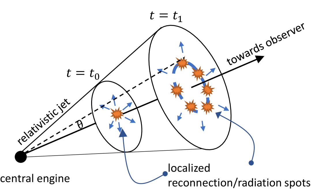
Figure 1: The illustration of the model

The observed specific flux of a GRB is (see derivation in the toy model paper, Yi et al. 2025a):

$$F_{\nu_{\rm obs}}(t_{\rm obs})=\frac{4\pi\Gamma}{D^{2}_{\rm{L}}}\int\int\mathcal{D}(\theta)^{3}j^{\prime}_{\nu_{\rm emt}^{\prime}}(r,t,\theta)\sin\theta d\theta r^{2}dr,$$ (1)

where $\Gamma$ is the Lorentz factor of the jet, $\mathcal{D}$ is the Doppler factor of the emitters, $j^{\prime}_{\nu^{\prime}}$ is the emissivity in the co-moving frame, $t$ is the time of emission in the central engine-rest frame, and $t_{\rm obs}$ is the time in the observer frame. $t$ is a function of $t_{\rm obs}$ and $\theta$ as:

$$t=\frac{t_{\rm obs}}{(1+z)(1-\beta\cos\theta)}+t_{0},$$ (2)

where $t_{0}=r_{0}/(\beta c)$ and $r_{0}$ is the radius of the initial reconnection, $\beta=v/c$ is the velocity of the jet with respect to the speed of light.

According to the dynamics of our model, the emissivity has the form:

$$j^{\prime}_{\nu_{\rm emt}^{\prime}}(r,t,\theta)=\delta(r-R(t))f(\nu,t,t_{\rm inj}(\theta)),$$ (3)

where $f(\nu^{\prime},t,t_{\rm inj}(\theta))$ denotes the spectrum of emitted photons at centre engine rest frame time $t$ due to electrons injected at $t=t_{\rm inj}$ at a certain ring $\theta$. The relation between $t_{\rm inj}$ and $\theta$ is (see the toy model paper, Yi et al. 2025a):

$$t_{\rm inj}=\frac{t_{0}}{1-\theta\beta\Gamma/\tilde{\beta}}.$$ (4)

Since $f(\nu_{\rm emt}^{\prime},t;t_{\rm inj})$ is nonzero only at $t\geq t_{\rm inj}$, and there is one-to-one function between $\theta$ and $t_{\rm inj}$, the integral over $\theta$ can be rewritten as integral over $t_{\rm inj}$ to a maximum value $t_{\rm max}$ corresponding to $t_{\rm obs}$. the above equation become:

$$F_{\nu_{\rm obs}}(t_{\rm obs})=\frac{2\pi\Gamma}{D^{2}_{\rm{L}}}\int^{t_{\rm max}(t_{\rm obs})}_{t_{0}}\mathcal{D}^{3}f(\nu_{\rm emt}^{\prime},t;t_{\rm inj})R^{2}\cos\theta\sin\theta\frac{d\theta}{dt_{\rm inj}}dt_{\rm inj}.$$ (5)

In the above equation, the integration upper limit $t_{\rm max}$ is solely determined by $t_{\rm obs}$. The relation between $t_{\rm max}$ and $t_{\rm obs}$ is found with the following two equations:

$$t_{\rm obs} = (1+z)(1-\beta\cos{\theta})(t_{\rm max}-t_{0})$$ (6)

$$\theta = \frac{1-t_{0}/t_{\rm max}}{\beta\Gamma/\tilde{\beta}}.$$ (7)

The Doppler factor $\mathcal{D}$ is a function of $\theta$, and the latter is a function of $t_{\rm inj}$:

$$\theta=\frac{1-t_{0}/t_{\rm inj}}{\beta\Gamma/\tilde{\beta}}.$$ (8)

$\nu^{\prime}$ is determined by $\nu_{\rm obs}$ and $\mathcal{D}$, $\nu^{\prime}=\nu_{\rm obs}/((1+z)\mathcal{D})$, therefore also a function of $t_{\rm inj}$ that takes place in the integral. $R$ is function of $t$:

$$R=\beta ct.$$ (9)

However $t$ is also determined by $t_{\rm obs}$ and $\theta$ as:

$$t=t_{0}+\frac{t_{\rm obs}}{(1+z)(1-\beta\cos\theta)}.$$ (10)

Since $\theta$ has a one-to-one mapping to $t_{\rm inj}$, $t$ is a function of $t_{\rm obs}$ and $t_{\rm inj}$: $t(t_{\rm obs},t_{\rm inj})$.

The key is to find the formula of $f(\nu_{\rm emt}^{\prime},t;t_{\rm inj})$. In order to do that, we need to get the spectrum of the electrons $dn_{e}(\gamma^{\prime}_{e},t;t_{\rm inj})/d\gamma^{\prime}_{e}$, where $\gamma^{\prime}_{e}$ is the Lorentz factor of the electron in the co-moving frame.

We assume that the $\gamma^{\prime}_{e}$ follows a power law at injection instant:

$$dn_{e}(\gamma^{\prime}_{e},t_{\rm inj},t_{\rm inj})/d\gamma^{\prime}_{e}=\dot{n}_{\rm e}(t_{\rm inj})\kappa{\gamma^{\prime}_{e}}^{-p}\delta t_{\rm inj},$$ (11)

where $\dot{n}_{\rm e}(t_{\rm inj})$ is the electron injection rate density. In the above equation, $\kappa$ is the normalization factor of the probability density so that:

$$\int_{{\gamma}_{m}}^{\infty}\kappa{\gamma^{\prime}_{e}}^{-p}=1,$$ (12)

where $\gamma_{m}$ is the minimum electron Lorentz factor at injection. By normalizing the power-law distribution, $\kappa=\frac{p-1}{{\gamma}_{m}^{1-p}}$. The kinetic energy density of the injected electrons are ($p>2$):

$$\epsilon=\kappa\dot{n}_{e}\delta t_{\rm inj}m_{e}c^{2}\int^{\infty}_{{\gamma}_{m}}{\gamma^{\prime}_{e}}^{1-p}d\gamma^{\prime}_{e}=\frac{p-1}{p-2}\gamma_{m}\dot{n}_{e}\delta t_{\rm inj}m_{e}c^{2}.$$ (13)

In this scenario, the electrons are accelerated by the reconnection of the local toroidal magnetic field. Therefore:

$$\epsilon=\frac{{B^{\prime}}^{2}}{4\pi},$$ (14)

where $B^{\prime}$ is the magnetic field strength in the co-moving frame. According to the conservation of the toroidal magnetic field energy, $B$ scaled with $1/r$ as:

$$B^{\prime}=B_{0}^{\prime}\frac{r_{0}}{r}.$$ (15)

As a result, $\dot{n}_{e}$ can be found out to be:

$$\dot{n}_{e}=\frac{{B^{\prime}}^{2}}{4\pi m_{e}c^{2}}\frac{p-2}{p-1}\frac{1}{\gamma_{m}}.$$ (16)

For each electron with Lorentz factor $\gamma^{\prime}_{e}$, its energy evolution follows (Uhm & Zhang, 2014):

$$\frac{d}{dt^{\prime}}y=\frac{\sigma_{T}}{6\pi m_{e}c}{B^{\prime}}^{2}-\frac{1}{3}y\frac{d\ln n_{e}}{dt^{\prime}},$$ (17)

where $y\equiv 1/\gamma^{\prime}_{e}$. The first term on the right-hand side of the above equation corresponds to the synchrotron cooling, while the second term corresponds to the adiabatic cooling. Since $n_{e}\propto r^{-2}$, the above adiabatic term becomes:

$$\frac{dy}{dt^{\prime}}|_{\rm adiab}=\frac{2\beta c\Gamma}{3}\frac{y}{r}.$$ (18)

Following Uhm & Zhang (2014), we find $dn_{e}(\gamma^{\prime}_{e},t;t_{\rm inj})/d\gamma^{\prime}_{e}$ by the following method:

1. In an array of $\gamma^{\prime}_{e}$ bins from $\gamma^{\prime}_{m}$ to $\gamma^{\prime}_{M}$, we assign the number of electrons according to equation (11);

2. For each bin at $\gamma^{\prime}_{e}$, we evolve the energy of electron according to equation (18) to time $t$;

3. At time $t$, we redistribute the new $\gamma^{\prime}_{e}(t)$ into the bins, and assign weight according to the number of electrons in its initial bin.

After $dn_{e}(\gamma^{\prime}_{e},t;t_{\theta})/d\gamma^{\prime}_{e}$ is known, we integrate the synchrotron radiation contributed by electrons at each $\gamma^{\prime}_{e}$:

$$f(\nu_{\rm emt}^{\prime},t;t_{\theta})=\Delta r^{\prime}\int^{\gamma^{\prime}_{M}}_{\gamma^{\prime}_{m}}P_{\text{syn}}(\nu_{\rm emt}^{\prime},B^{\prime},\gamma^{\prime}_{e})\frac{dn_{e}(\gamma^{\prime}_{e},t;t_{\theta})}{d\gamma^{\prime}_{e}}d\gamma^{\prime}_{e},$$ (19)

where the synchrotron radiation power for single electron at $\gamma^{\prime}_{e}$ is:

$$P_{\text{syn}}(\nu_{\rm emt}^{\prime},B^{\prime},\gamma^{\prime}_{e})=\frac{\sqrt{3}e^{3}B^{\prime}}{m_{\mathrm{e}}c^{2}}\cdot\frac{\nu_{\rm emt}^{\prime}}{\nu_{c}}\cdot\int_{\nu/\nu_{c}}^{\infty}\mathrm{K}_{5/3}(x)\,\mathrm{d}x$$ (20)

where $\text{K}_{5/3}$ denotes the modified Bessel function, and $\nu_{c}$ is the critical frequency related with $\gamma^{\prime}_{e}$:

$$\nu_{c}=\frac{3eB^{\prime}{\gamma^{\prime}_{e}}^{2}}{4\pi m_{\mathrm{e}}c}.$$ (21)

$\Delta r^{\prime}$ is the thickness of the shell of dissipation, in our setting, $\Delta r^{\prime}\ll R/\Gamma$, corresponding to a thin shell in the comoving frame.

Taking equation (19) into equation (5) allows us to obtain the observed specific flux as a function of time and photon energy.

3 Reproducing the spectrum-time features of individual bursts

With $F_{\nu_{\rm obs}}(t_{\rm obs})$ known, the light curve of a GRB in different energy bands can be obtained by integrating the specific flux over the corresponding energy band. The spectrum of a GRB at a certain time interval can be obtained by averaging $F_{\nu_{\rm obs}}(t_{\rm obs})$ over the time interval. In the above derivation, we assume the emissivity of the GRB is smooth. In reality, the localized reconnection and radiation spots can be randomly distributed in the jet front in discrete latitudes and azimuth angles. In order to simulate the discrete nature of the radiation spots, we replace the integral over $t_{\rm inj}(\theta)$ in Equation (5) with a summation over a randomly distributed $\theta_{i}$: $\int dt_{\rm inj}\rightarrow\sum\Delta t_{{\rm inj},i}$, where $\Delta t_{i}=t_{\rm inj,i+1}(\theta_{i+1})-t_{\rm inj,i}(\theta_{i})$, and $\cos\theta_{i}$ is uniformly randomly distributed in the range of $[\cos\theta_{\rm max},1]$. We denote the number of radiation rings as $N_{\rm ring}$.

As an example, we take the following parameters to simulate a GRB with our model: $\Gamma=180$, $r_{0}=2\times 10^{15}$cm, $B_{0}^{\prime}=1$G, $p=2.8$, $\gamma_{m}=2\times 10^{5}$, $\gamma_{M}=10^{7}$, $z=0.06$, $\Delta r^{\prime}=10^{10}$cm and $N_{\rm ring}=200$. The choice of model parameters in our simulation is motivated by both observational constraints and theoretical considerations. The Lorentz factor $\Gamma$, initial radius $r_{0}$, and magnetic field $B_{0}^{\prime}$ are selected to be representative of typical values. The electron distribution parameters ($\gamma_{m}$, $\gamma_{M}$, $p$) are chosen to reflect the range commonly required to reproduce observed GRB spectra (Uhm & Zhang, 2014). The number of radiation rings $N_{\rm ring}$ is set to balance the observed diversity in light curve smoothness and variability. Our results are robust to moderate changes within a reasonable ranges, and the qualitative features of the model persist. In Figure 2, we show the simulated light curve of the GRB in 7 different energy bands, i.e., 6-30 keV, 30-70 keV, 70-100 keV, 100-150 keV, 150-200 keV, 200-500 keV and 500-1000 keV. The light curves exhibit a typical FRED profile, with the peak time and width evolving with energy. We fit the light curves with a FRED function defined in Norris et al. (2005):

$$F(t)\propto\exp\left(-(\frac{t-t_{0}}{t_{d}}+\frac{t_{r}}{t-t_{0}})\right).$$ (22)

In this formulation, we define the peaking time delay as $t_{p}=\sqrt{t_{r}t_{d}}$, and the pulse time scale (a simple proxy of the pulse width) as $t_{w}=t_{r}+t_{d}$. The fitted $t_{p}$ and $t_{w}$ as a function of energy are shown in Figure 3. The value of the energy is the geometrical mean of each energy band, while the error bar of energy is the width of the energy band. The best fit FRED profiles are plotted along with the light curves in Figure 2.

It can be seen that the energy dependent of $t_{p}$ and $t_{w}$ can be fitted with a power law, with the fitted power indices being both $-0.39$.

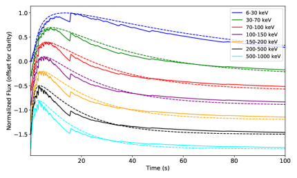
Figure 2: The simulated light curve of a GRB in 7 different energy bands, i.e., 6-30keV, 30-70keV, 70-100keV, 100-150keV, 150-200keV, 200-500keV and 500-1000keV.

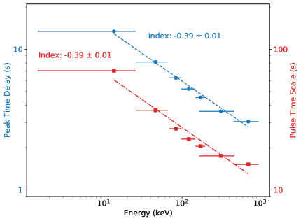
Figure 3: The peak time and width of the simulated GRB light curves as a function of energy. The best fit power law are plotted as dashed lines.

The corresponding spectrum of the GRB at 7 different time windows are shown in figure 4. The spectra exhibit a typical Band function shape, with the peak energy $E_{p}$ evolving with time.

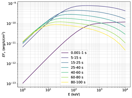
Figure 4: The simulated GRB spectra at 7 different time windows, corresponding to the light curves in figure 2.

It is worth mentioning that not only the overall self-similar FRED profile can be reproduced, but also it is clearly shown that these FRED profile are composed of many individual pulses, which are aligned in different energy bands, as in the observation of GRB 230307A (Yi et al., 2025b). These individual pulses correspond to the localized radiation spots in the random discrete rings. The duration of these individual pulses also shows systematic trend of increasing with time, which is consistent with the recent findings in GRB 230307A (Maccary et al., 2025). In our model, this trend is a natural outcome of the decreasing of the Doppler factor of individual radiation rings with time, as the radiation area propagates outward to higher latitudes. Furthermore, we also simulate the instantaneous spectrum $\nu f_{\rm\nu}$ of the simulated GRB and find the evolution of $E_{p}$. We plot $E_{p}-t$ along with the energy integrated light curve in figure 5. It can be seen that, in addition to the general decrease in long time scale, $E_{p}$ tracks the intensity of the GRB in short time scale, which is common in GRBs and also consistent with the observation of GRB 230307A (Sun et al., 2023). This local intensity tracking can be explained in our framework as the cooling of the electrons in the local radiation spots.

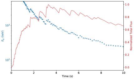
Figure 5: The $E_{p}$ as function of time, along with the energy integrated light curve of the simulated GRB.

4 The empirical relationships between physical parameters and observational parameters of single FRED GRBs

Given a set of model parameters, we can accurately reproduce the spectrum-time features of a single FRED GRB as demonstrated in the previous section. With a distribution of model parameters, we can further generate a population of such GRBs. The distribution of the model parameters are set as follows: $\Gamma$ is uniformly distributed from 100 to 500; $r_{0}$ is uniformly distributed in log-space from $5\times 10^{14}$ cm to $5\times 10^{15}$ cm; $B_{0}^{\prime}$ is uniformly distributed from 3 to 30 G; $\gamma_{m}$ is log-uniformly distributed from $10^{4}$ to $10^{5}$, $\gamma_{M}$ is log-uniformly distributed from $10^{7}$ to $10^{8}$. From the simulated population of size 1000, we calculate the T₉₀ of the energy-integrated light curve, the peak energy $E_{p}$ of the time averaged spectrum, and $t_{p}-E$ and $t_{w}-E$ power indices. In figure 6, we show the distribution of the $t_{p}-E$ and $t_{w}-E$ power indices. It can be seen that the indices are clustered around the diagonal line, where the both indices are identical, corresponding to perfect self-similar profiles. Therefore, a self-similar FRED of such GRBs is a natural outcome of our mechanism. The T₉₀ and $E_{p}$ of the simulated population are shown in figure 7. It can be seen from the distribution of T₉₀ that, a lot of the single FRED GRBs are short duration GRBs, consistent with the impulsive central engine activity expected for Type-I GRBs. Still, there are some long duration GRBs with T₉₀ of several tens of seconds, which explains the existence of long duration Type-I bursts such as GRB 211211A and 230307A (Rastinejad et al., 2022; Levan et al., 2024; Wang et al., 2025; Tan et al., 2025). In figures 6, we also superpose the observed parameters from a set of recently discovered single FRED GRBs (See details in the Appendix: a new catalogue of general single FRED GRBs). As can be seen, the data points are also clustered around the diagonal line, indicating self-similar profiles, which is consistent with our simulation results. However, there seems to be an excess of outliers with $t_{p}-E$ index larger than $t_{w}-E$ index. This may suggest a different distribution of the physical parameters than the one we assumed in our simulation. More data and more detailed analysis are needed to clarify this issue in the future.

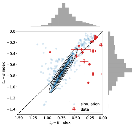
Figure 6: The distribution of the $t_{p}-E$ and $t_{w}-E$ power indices of the simulated population of single FRED GRBs. The dashed line is the diagonal line where the two indices are identical. The red points are the observed parameters from a new catalogue of single FRED GRBs (See details in the Appendix: a new catalogue of general single FRED GRBs).

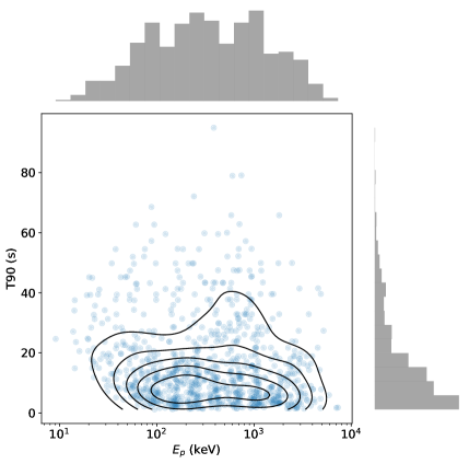
Figure 7: The distribution of T₉₀ and $E_{p}$ of the simulated population of single FRED GRBs.

We further fit an empirical relation between the physical parameters and the observational parameters of the simulated population. The empirical relation is defined as:

$$\vec{X}_{\rm obs}=\vec{Y}_{\rm obs}\mathbf{A}+\vec{B},$$ (23)

where

$$\vec{X}_{\rm{obs}}=[\log_{10}\text{T}_{90},\log_{10}E_{p},\text{index}_{t_{p}},\text{index}_{t_{w}}],$$ (24)

$$\vec{Y}_{\rm{obs}}=[\log_{10}\Gamma,\log_{10}r_{0},\log_{10}B_{0}^{\prime},\log_{10}\gamma_{m},\log_{10}\gamma_{M}],$$ (25)

$\mathbf{A}$ is a $4\times 5$ matrix defining the linear coefficients, and $\vec{B}$ is a 4-dimensional vector of the intercepts. The best fit coefficients are:

$$\mathbf{A}=\begin{pmatrix}1.2&-0.2&0.2&1.7&-0.004\\ -1.5&0.8&0.1&0.3&-0.003\\ -0.4&0.1&-0.3&-0.3&0.006\\ -0.5&0.2&-0.4&-0.3&0.008\\ \end{pmatrix}$$ (26)

$$\vec{B}=\begin{pmatrix}-4.5\\ -9.4\\ 0.5\\ -0.1\\ \end{pmatrix}$$ (27)

In order the estimate the goodness of the empirical relation, we plot the observables calculated with the empirical relation against the ones calculated with the simulations in figure 8.

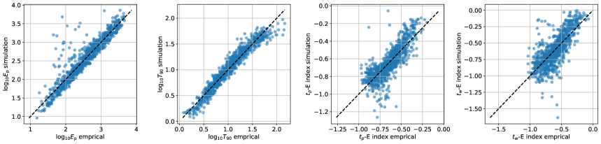
Figure 8: The comparison between the observables calculated with the empirical relation and the ones calculated with the simulations. The dashed lines are the diagonal lines where the two values are identical.

The empirical relation can be used to estimate the observables of a single FRED from our scenario with a set of physical parameters with much less computational cost. It can also be used to estimate the physical parameters of a single FRED GRB with its observables.

5 conclusions and discussions

In this paper, we have established a self-consistent physical model that attributes the peculiar self-similar FRED profile in GRBs, to the propagation of internal collision-caused perturbation in a magnetically dominated relativistic jet front. The initial perturbation are caused by an impulsive energy injection from the central engine and is localized. The perturbation then propagates outwards in a geometrically thin shell in the jet front, in the form of Alfvén waves. The perturbation propagates in concentric circles, and randomly triggers local magnetic reconnection and radiation at different latitudes, which results in the overall FRED profile of the GRB. The local radiation spots are also responsible for the individual pulses in the light curve, which are aligned in different energy bands.

In each localized radiation spot, energetic electrons are accelerated by the magnetic reconnection and then endures cooling from synchrotron radiation and adiabatic expansion as the ejecta moving forward. We derive the energy-time evolution of the GRB by solving the electron cooling and radiation equations at each local radiation spot.

All the features of single FRED GRBs can be reproduced with our model, including: 1. self-similar FRED profile, which is due to the concentric circle propagation of the perturbation; 2. multi-band aligned individual pulses, which is due to the random distribution of the local radiation spots; 3. overall hard-to-soft spectral evolution, which is due to the decreasing Doppler factor of the radiation spots as they propagate outward; 4. local intensity tracking, which is due to the cooling of the electrons in the local radiation spots. 5. A systematic trend of increasing duration of the individual pulses, which is due to the decreasing Doppler factor of the radiation spots as they propagate outward.

Furthermore, we conduct Monte Carlo simulations to study the population properties of such GRBs, given a distribution of physical parameters. We find that the $t_{p}-E$ and $t_{w}-E$ power indices are clustered around the diagonal line, which indicates that the self-similar FRED profile is a natural outcome of our model. The T₉₀ and $E_{p}$ of the simulated population are consistent with the observed single FRED GRBs, including both short and long duration bursts. We also establish an empirical relation between the physical parameters and the observables of single FRED GRBs, which can be used to estimate the observables from a set of physical parameters with much less computational cost, or vice versa.

In the observation, some single FRED GRBs exhibit smooth light curves, while others show high short time variability. In our model, the smoothness of the light curve is controlled by the number of local radiation spots. More radiation spots result in a smoother light curve, while fewer radiation spots lead to a more variable light curve. The variability can be further increased if there are minijets within each local radiation spot, as shown in the simulation studies (Zhang & Zhang, 2014; Shao & Gao, 2022).

In our model, the reproduction of a canonical FRED shape depends on two assumptions: 1. there is only one initial perturbation; 2. the initial location of the perturbation is close to the line of sight. If the initial perturbation is away from the line of sight, the profile will be distorted from the canonical FRED shape; if there are multiple initial perturbation on the other hands, the profile will be more complex, being the superposition of multiple distorted FRED profiles.

The radiation mechanism in this model is assumed to be pure synchrotron radiation. In reality, if the photons are partially thermalized when the radiation location is compact, the spectrum will be softer at the beginning of the burst, as observed in GRB 230307A (Sun et al., 2023).

From our study, it is clearly shown that the self-similar FRED profile of GRBs is reflecting the dissipation within the jet, rather than the activity history of the central engine. Therefore, the recent changing to the traditional merger-short/collapsar-long dichotomy of GRBs can be reconciled (Zhang, 2025). It is also elaborated why we believed that the composed self-similar FRED profile is a strong evidence of magnetically dominated jets.

There has been efforts to infer the central engine activity from the light curve of GRBs. However, as we pointed out here, the light curve of GRBs is not a direct reflection of the central engine activity, but rather a convolution of the response to the impulsive central engine activity and the history of the central engine activity. As a result, knowing the properties of such response is criucial for understanding the central engine activity. From a series of our studies (Yi et al., 2025b, a), we have shown that the self-similar FRED profile is such a response. Therefore, the long time activity history of the central engine can be accurately studied.

Appendix A A catalogue of general single FRED GRBs from Fermi/GBM

Here we present a catalogue of single FRED GRBs found in Fermi/GBM GRBs, and find their energy-dependence of pulse width and peak time.

To begin with, we extracted the lightcurves in four energy channels (i.e. 8-30 keV, 30-100 keV, 100-300 keV, 300-900 keV) for all cataloged Fermi/GBM GRBs (von Kienlin et al., 2020) using the archived Time-Tagged Event (TTE) data of all NaI detectors. Then the searching for single FRED sample is conducted by the following step:

1. We restrict our sample to GRBs with $T_{90}>2\,$s, as they are expected to exhibit more pronounced spectral lags, enabling a more robust determination of the energy dependence law. GRBs with a fluence less than $10^{-5}$ erg$\cdot$cm^-2 were also excluded, to ensure sufficient counts for reliable analysis.

2. The lightcurve of 300-900 keV (the hardest energy range we used) is rebinned with a time resolution of 0.5 s from T₀-T₉₀ to T₀+3T₉₀, where T₀ set as the trigger time for each GRBs.

3. Then this rebinned 300-900 keV lightcurve is fitted by a FRED model (Norris et al., 2005), which is stated as Equation 22, superposed on a one-order polynomial background by the same MCMC approach with Yi et al. (2025b). GRBs with residuals less than 5 are selected as part of single FRED GRBs sample.

4. The rebinned 300-900 keV lightcurve in step (2) is also used to perform peak searching by MEPSA (Guidorzi, 2015). GRBs with only one pulse identified are contributed to the other part of the single FRED GRBs sample.

A total of 28 single pulse GRBs are collected based on the above steps. Then we fitted the four channel lightcurves of these 28 GRBs with the same process in step (3). We set a prior of the parameter imposing that both the rise time scale and decay time scale should shorter than T₉₀. We excluded GRBs whose parameters are not well constrained, and left 17 GRBs in our final sample.

The pulse width and peak time are deduced based on the parameters of FRED with the same definition in Yi et al. (2025b), and fitted by powerlaw to get their energy-dependence (i.e. the slope) respectively, as shown in the figure 6.

Table 1: Sample of general single FRED GRBs

GRB name	T0	Slope of tp	Slope of tw
GRB 130304A	2013-03-04T09:49:53.099	-0.37${}^{+0.18}_{-0.16}$	-0.33${}^{+0.03}_{-0.03}$
GRB 130704A	2013-07-04T13:26:07.253	-0.42${}^{+0.00}_{-0.00}$	-0.26${}^{+0.00}_{-0.00}$
GRB 140723A	2014-07-23T01:36:30.728	-0.33${}^{+0.07}_{-0.07}$	-0.55${}^{+0.04}_{-0.04}$
GRB 160101A	2016-01-01T00:43:53.610	-0.12${}^{+0.01}_{-0.01}$	-0.12${}^{+0.01}_{-0.01}$
GRB 161206A	2016-12-06T01:32:28.077	-0.14${}^{+0.01}_{-0.01}$	-0.12${}^{+0.01}_{-0.01}$
GRB 170921B	2017-09-21T04:02:11.511	-0.93${}^{+0.01}_{-0.01}$	-0.38${}^{+0.01}_{-0.01}$
GRB 171210A	2017-12-10T11:49:15.261	-0.26${}^{+0.01}_{-0.01}$	-0.93${}^{+0.01}_{-0.01}$
GRB 180426A	2018-04-26T13:11:00.846	-0.03${}^{+0.03}_{-0.03}$	-0.25${}^{+0.03}_{-0.03}$
GRB 180806A	2018-08-06T22:38:59.661	-0.13${}^{+0.01}_{-0.01}$	-0.08${}^{+0.01}_{-0.01}$
GRB 190222A	2019-02-22T12:53:27.151	-0.46${}^{+0.04}_{-0.04}$	-0.45${}^{+0.03}_{-0.03}$
GRB 190604A	2019-06-04T10:42:37.054	-0.14${}^{+0.01}_{-0.01}$	-0.14${}^{+0.01}_{-0.01}$
GRB 200607B	2020-06-07T22:06:31.425	-0.17${}^{+0.14}_{-0.14}$	-0.77${}^{+0.03}_{-0.02}$
GRB 211116A	2021-11-16T14:03:53.348	-0.36${}^{+0.03}_{-0.03}$	-0.39${}^{+0.02}_{-0.02}$
GRB 221221A	2022-12-21T22:39:30.568	-0.19${}^{+0.03}_{-0.03}$	-0.19${}^{+0.02}_{-0.02}$
GRB 230402A	2023-04-02T07:32:35.956	-0.24${}^{+0.02}_{-0.02}$	-0.59${}^{+0.02}_{-0.02}$
GRB 230621A	2023-06-21T23:45:24.826	-0.17${}^{+0.04}_{-0.04}$	-0.35${}^{+0.03}_{-0.03}$
GRB 240914B	2024-09-14T07:09:47.313	-0.10${}^{+0.01}_{-0.01}$	-0.10${}^{+0.01}_{-0.01}$

References

- Bazzanini et al. (2024) Bazzanini, L., Ferro, L., Guidorzi, C., et al. 2024, A&A, 689, A266
- Fenimore et al. (1996) Fenimore, E. E., Madras, C. D., & Nayakshin, S. 1996, ApJ, 473, 998
- Guidorzi (2015) Guidorzi, C. 2015, Astronomy and Computing, 10, 54
- Hakkila et al. (2008) Hakkila, J., Giblin, T. W., Norris, J. P., Fragile, P. C., & Bonnell, J. T. 2008, ApJ, 677, L81
- Kobayashi et al. (1997) Kobayashi, S., Piran, T., & Sari, R. 1997, ApJ, 490, 92
- Kocevski et al. (2003) Kocevski, D., Ryde, F., & Liang, E. 2003, ApJ, 596, 389
- Kouveliotou et al. (1992) Kouveliotou, C., Paciesas, W. S., Fishman, G. J., Meegan, C. A., & Wilson, R. B. 1992, in NASA Conference Publication, Vol. 3137, NASA Conference Publication, ed. C. R. Shrader, N. Gehrels, & B. Dennis, 61–68
- Levan et al. (2024) Levan, A. J., Gompertz, B. P., Salafia, O. S., et al. 2024, Nature, 626, 737
- Liang et al. (2006) Liang, E.-W., Zhang, B.-B., Stamatikos, M., et al. 2006, ApJ, 653, L81
- Maccary et al. (2025) Maccary, R., Guidorzi, C., Maistrello, M., et al. 2025, arXiv e-prints, arXiv:2509.05628
- Maistrello et al. (2025) Maistrello, M., Ferro, L., Bazzanini, L., Maccary, R., & Guidorzi, C. 2025, A&A, 697, A76
- Maxham & Zhang (2009) Maxham, A., & Zhang, B. 2009, ApJ, 707, 1623
- Moradi et al. (2024) Moradi, R., Wang, C. W., Zhang, B., et al. 2024, ApJ, 977, 155
- Nathanail et al. (2014) Nathanail, A., Basilakos, S., & Contopoulos, I. 2014, in Proceedings of Swift: 10 Years of Discovery (SWIFT 10, 90
- Norris et al. (2005) Norris, J. P., Bonnell, J. T., Kazanas, D., et al. 2005, ApJ, 627, 324
- Norris et al. (1996) Norris, J. P., Nemiroff, R. J., Bonnell, J. T., et al. 1996, ApJ, 459, 393
- Peng et al. (2012) Peng, Z. Y., Zhao, X. H., Yin, Y., Bao, Y. Y., & Ma, L. 2012, ApJ, 752, 132
- Rastinejad et al. (2022) Rastinejad, J. C., Gompertz, B. P., Levan, A. J., et al. 2022, Nature, 612, 223
- Shao & Gao (2022) Shao, X., & Gao, H. 2022, ApJ, 927, 173
- Sun et al. (2023) Sun, H., Wang, C.-W., Yang, J., et al. 2023, arXiv preprint arXiv:2307.05689
- Tan et al. (2025) Tan, W.-J., Wang, C.-W., Zhang, P., et al. 2025, arXiv e-prints, arXiv:2504.06616
- Uhm & Zhang (2014) Uhm, Z. L., & Zhang, B. 2014, Nature Physics, 10, 351
- Uhm et al. (2018) Uhm, Z. L., Zhang, B., & Racusin, J. 2018, ApJ, 869, 100
- von Kienlin et al. (2020) von Kienlin, A., Meegan, C. A., Paciesas, W. S., et al. 2020, ApJ, 893, 46
- Wang et al. (2025) Wang, C.-W., Tan, W.-J., Xiong, S.-L., et al. 2025, ApJ, 979, 73
- Yan et al. (2024) Yan, Z.-Y., Yang, J., Zhao, X.-H., Meng, Y.-Z., & Zhang, B.-B. 2024, ApJ, 962, 85
- Yi et al. (2025a) Yi, S.-X., Yorgancioglu, E. S., Xiong, S. L., & Zhang, S. N. 2025a, Journal of High Energy Astrophysics, 47, 100359
- Yi et al. (2025b) Yi, S. X., Wang, C. W., Shao, X., et al. 2025b, ApJ, 985, 239
- Zhang (2025) Zhang, B. 2025, Journal of High Energy Astrophysics, 45, 325
- Zhang & Yan (2010) Zhang, B., & Yan, H. 2010, The Astrophysical Journal, 726, 90
- Zhang & Zhang (2014) Zhang, B., & Zhang, B. 2014, ApJ, 782, 92