Deep Synoptic Array Science: Searching for Long Duration Radio Transients with the DSA-110

Abstract

We describe the design and commissioning tests for the DSA-110 Not-So-Fast Radio Burst (NSFRB) search pipeline, a 1.4 GHz image-plane single-pulse search sensitive to 134 ms$-$160.8 s radio bursts. Extending the pulse width range of the Fast Radio Burst (FRB) search by 3 orders of magnitude, the NSFRB search is sensitive to the recently-discovered Galactic Long Period Radio Transients (LPRTs). The NSFRB search operates in real-time, utilizing a custom GPU-accelerated search code, cerberus, implemented in Python with JAX. We summarize successful commissioning sensitivity tests with continuum sources and pulsar B0329+54, estimating the $6\sigma$ flux (fluence) threshold to be $\sim 290\,$mJy ($\sim 40$ Jy ms). Future tests of recovery of longer timescale transients, e.g. CHIME J1634+44, are planned to supplement injection testing and B0329+54 observations. An offline DSA-110 NSFRB Galactic Plane Survey was conducted to search for LPRTs, covering $-3.5^{\circ}<b<5.7^{\circ}$ and $141^{\circ}<l<225^{\circ}$ ($\sim 770\,$square degrees) in Galactic coordinates. We estimate an upper limit Poissonian burst rate $\sim 1\,$hr^-1 per square degree ($\sim 7$ hr^-1 per $3^{\circ}\times 3^{\circ}$ survey grid cell) maximized across the inner $|b|<0.25^{\circ}$ of the surveyed region. By imposing the $\sim 290\,$mJy flux limit on two representative models (the magnetar plastic flow model and the White Dwarf-M Dwarf binary model), we reject with 95% confidence the presence of White Dwarf-M Dwarf binary LPRTs with periods between $\sim 10-70$ s within $\sim 95\%$ of the surveyed region. Combined with the prevalence of LPRTs in the Galactic Plane, our results motivate further consideration of both White Dwarf-M Dwarf binary models and isolated magnetar models. We will continue to explore novel LPRT search strategies during real-time operations, such as triggered periodicity searches and additional targeted surveys.

1 Introduction

Radio pulsar searching is entering a new exploratory phase; traditional single-dish telescope searches such as the Pulsar Arecibo L-band Feed Array (PALFA), Parkes Multi-beam Survey (PMBS), and Five-Hundred Metre Aperture Spherical Telescope (FAST) have utilized multi-beam receivers to discover roughly 2/3 of the $\sim 4000$ known Galactic pulsars (R. N. Manchester et al., 2005, 2001; J. Han et al., 2021; Y. Li et al., 2025). Over the past decade, the TRAnsients and PUlsars with MeerKAT (TRAPUM; E. Carli et al., 2024), the Canadian Hydrogen Intensity Mapping Experiment Pulsar (CHIME/PULSAR; F. A. Dong et al., 2023) backend, the LOw-Frequency ARray (LOFAR) Tied-Array All-Sky Survey (LOTAAS E. van der Wateren et al., 2023), and Very Large Array (VLA) realfast system (C. Law et al., 2018), among others, have demonstrated that radio interferometers can achieve competitive sensitivities to single-dish telescopes with higher localization precision and less-costly antennas. Beyond contributing $\sim 500$ additional pulsars, these arrays have been essential for follow-up imaging to identify and associate Supernova Remnants (SNRs), Pulsar Wind Nebulae (PWNe), long-duration afterglows, and Persistent Radio Sources (PRS) of both pulsars and extragalactic radio transients (e.g. B. M. Gaensler et al., 2005; G. Bruni et al., 2025; W. Cotton et al., 2024). However, these surveys have typically targeted pulsars with rotation periods $\lesssim 10$ seconds out of necessity. Fast Fourier-domain search strategies require long integration times to remain sensitive to periods beyond second-scales, and suffer from low-frequency red noise, making them impractical targets (S. M. Ransom, 2001; S. Singh et al., 2022). Periodic transients with longer rotation periods (seconds to minutes), such as radio magnetars, Rotating Radio Transients (RRATs), and White Dwarf-M Dwarf binaries (either non-tidally-locked intermediate polars like AR Scorpii or tidally-locked non-accreting polars) were instead identified through serendipitous imaging surveys or follow-up of their high-energy counterparts (e.g. S. D. Hyman et al., 2005; M. Caleb et al., 2022a; T. Marsh et al., 2016).

The recent discovery of a dozen Galactic radio sources with unusually long pulse periods between $\sim 20$ seconds$-8.7$ hours and low $\lesssim 10\%$ duty cycles have begun to reveal an abundant unconstrained parameter space (e.g. N. Hurley-Walker et al., 2022; I. de Ruiter et al., 2025; C. Horváth et al., 2025; Y. Men et al., 2025; C. Tan et al., 2018). These so-called “Long-Period Radio Transients” (LPRTs, or LPTs) exhibit some properties characteristic of neutron stars, such as high polarization fractions, polarization position angle (PA) swings, temporal sub-structure, and un-detectable optical/IR (OIR) emission (D. Mitra et al., 2023; M. Kramer et al., 2024; V. Radhakrishnan & D. J. Cooke, 1969; A. Chrimes et al., 2022). However, at least two LPRTs, ILT J1101+5521 ($P=2.1$ hours) and GLEAM-X J0704-37 ($P=2.9$ hours) reside in binaries with M-dwarf companions, with blue optical excess suggesting they are White Dwarfs (I. de Ruiter et al., 2025; N. Hurley-Walker et al., 2024). While the remaining sample have no clear M-Dwarf companions, the recent discovery of a secondary $P=8.74$ hr period of GPM J1839-10 solely from radio timing suggest the White-Dwarf-M-Dwarf interpretation may extend to OIR-quiet candidates (C. Horváth et al., 2025; Y. Men et al., 2025). Nonetheless, a plethora of both neutron star and White Dwarf-M Dwarf binary models have been proposed to explain these new phenomena (e.g. P. Beniamini et al., 2023, 2020; A. Cooper & Z. Wadiasingh, 2024; Y. Qu & B. Zhang, 2025).

LPRTs’ rapid emergence has spurred the development of novel search strategies on an accelerated timescale. The GaLactic and Extragalactic All-sky Murchison Wide-field Array (MWA)-Extended (GLEAM-X) survey’s first two discoveries (GLEAM-X J1627-52 and GPM J1839-10) were found as single pulses at low frequencies ($72-231$ MHz) by differencing incoherently summed visibilities from 4096 antennas at 0.5 s time resolution (N. Hurley-Walker et al., 2022, 2023). These were followed by ASKAP’s (1248 MHz) PSR J0901-4046, LOFAR’s PSR J0250+5854 (135 MHz), CHIME/FRB’s (400-800 MHz) CHIME J0630+25 and CHIME J1634+44, all of which were discovered as single-pulses in second and millisecond resolution beamformed visibilities (M. Caleb et al., 2022b; F. A. Dong et al., 2025a, b; C. Tan et al., 2018). These beamformed discoveries resulted in higher resolution ($\sim$arcsecond-to-arcminute) initial localizations, enabling immediate radio and multi-wavelength follow-up. In addition, ASKAP’s and MeerKAT’s L-band observations confirmed that LPRTs are detectable and discoverable at higher frequencies, where propagation effects like scattering in the Interstellar Medium (ISM) are less pronounced. Notably, all LPRT discoveries have been via single-pulses or sub-pulses rather than folding on trial rotation periods.

Perhaps most promising is the discovery of four ASKAP LPRTs (ASKAP J1755-2527, ASKAP J1935+2148, ASKAP J1839-0756, ASKAP/DART-J1832-0911), LOFAR’s ILT J1101+5521, and GLEAM-X J0704-37 using second-duration radio image differencing pipelines (Z. Wang et al., 2025a; D. Li et al., 2024; Y. Lee et al., 2025; M. Caleb et al., 2024; I. de Ruiter et al., 2025; S. J. McSweeney et al., 2025; D. Dobie et al., 2024). Radio imaging consists of binning the U-V (East-West and North-South coordinates of each antenna pair’s separation) visibility coordinates on a grid and applying a 2-dimensional FFT. This is much faster than visibility beamforming and is mathematically identical, though some resolution and flux sensitivity are lost via the gridding process. The image-plane LPRT detections demonstrate that this sensitivity loss is negligible for LPRT timescales (seconds-to-minutes), motivating the development of real-time LPRT image plane search pipelines. Such systems are either under development or beginning commissioning observations, including the CHIME/SLOW pipeline (J. Huang et al., in prep.) and the Commensal Real-time ASKAP Fast-Transients Coherent (CRACO) Upgrade (Z. Wang et al., 2025b).

In this paper, we introduce the Deep Synoptic Array’s (DSA-110) radio telescope’s Not-So-Fast Radio Burst (NSFRB) pipeline, an image-plane single-pulse search for LPRTs on 0.134-160.8 second timescales. The NSFRB system builds on the existing real-time Fast Radio Burst (FRB) search, which has discovered $\sim 60$ FRBs and localized $\sim 30$ to host galaxies with arcsecond-scale precision (V. Ravi et al., 2023; C. J. Law et al., 2024; K. Sharma et al., 2024). In Section 2 we describe the NSFRB system design and search pipeline; in Section 4 we report the results of a pilot DSA-110 NSFRB Galactic Plane Survey (DN-GPS); in Section 5 we discuss the sensitivity limits placed on LPRT emission in the Galactic Plane, and its implications for the White Dwarf binary model; in Section 6 we conclude with next steps, specifically the real-time search which is currently underway.

2 NSFRB System Design

The DSA-110 is a 96-antenna drift-scan radio interferometer at the Owens Valley Radio Observatory (OVRO) in Big Pine, CA. Details on the 64-antenna deployment and commissioning FRB survey can be found in V. Ravi et al. (2023). The array was completed in early 2025 by supplementing the East-West row of 47 “core” antennas with a 35-antenna North-South arm, enabling real-time localization of radio sources without incorporating the 14 long-baseline “outrigger” antennas. The antenna design, RF signal chain, baseband processing, and general compute resource layout remain largely similar to the 64-antenna deployment, and will not be detailed here. The revised visibility correlator, bandpass calibration procedures, and the FRB search pipeline will be discussed in detail elsewhere (Ravi et al., in prep.) For this work, we focus on components specific to the NSFRB system. Code for the NSFRB search is public at https://github.com/dsa110/dsa110-nsfrb, all of which is implemented using Python, leveraging the JAX library to deploy GPU tasks. An ETCD server is used to manage alerts and coordination between compute nodes. Figure 1 shows the full real-time system diagram, which we describe in the next sub-sections.

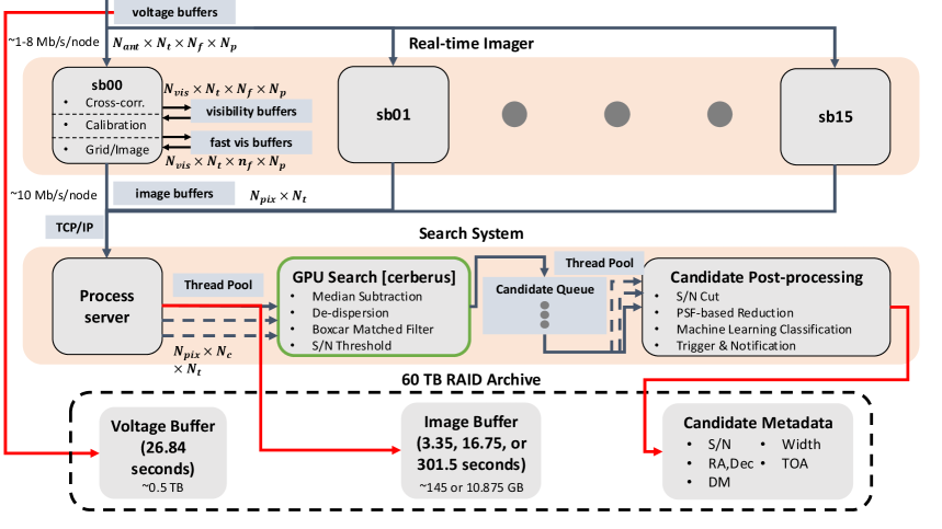
Figure 1: Diagram of the NSFRB Search System. Voltages for $N_{\rm ant}=97$ antennas, $N_{t}=25$ time samples, $N_{p}=2$ polarizations, and $N_{f}=384$ frequency channels are pulled from a rotating PSRDADA buffer, cross-correlated, down-channelized to $n_{f}=8$, and calibrated. $N_{\rm pix}=301\times 301$ images are formed for each of $N_{c}=16$ sub-bands and sent to the Process Server which assigns search and post-processing tasks. Image data and candidate metadata are saved to disk along with 26.8-second of voltage data triggered from the PSRDADA buffer if candidates above the $6\sigma$ threshold are identified. We outline in green the post-processor which is not required to operate in real-time.

2.1 Fringe-Stopping and Imaging

The 187.5 MHz observing band, centered on 1.4 GHz, is split into $16\times 11.7$ MHz sub-bands, each processed on a single compute node. Each node’s correlator outputs dual-polarization $N_{\rm base}=4656$ cross-correlated visibilities as $384\times 30.5$ kHz Nyquist-sampled ($32.7\mu$s) channels to a PSRDada buffer (W. van Straten et al., 2021). For the NSFRB search, these are calibrated and fringe-stopped to the current meridian position in $\sim 3.35$ second (102400 samples) chunks, down sampling to $134\,$ms resolution (25 samples) and $8\times 1.46$ MHz channels. The 3.35 s fringe-stopping interval is selected to maintain point-source coherence; the fringe-timescale of the array is:

$$t_{F}=648000{\rm s}\frac{\lambda_{c}}{\pi b_{\rm max}15\cos{(\delta)}}\approx\frac{1.05\,{\rm s}}{\cos{(\delta)}}$$ (1)

for the DSA-110, $b_{\rm max}=2.6\,$km, $\lambda_{c}=20$ cm, where $\delta$ is the declination (e.g. A. R. Thompson et al., 2017). The array operates in drift-scan mode (no azimuthal slew) at $\delta=71.6^{\circ}$ during normal operations, making the nominal fringe rate $t_{F0}\approx 3.36\,$s.

Fringe-stopped visibilities are written to a 14.9 MB buffer read by the correlator node imager, which grids visibilities with baseline lengths $b>b_{\rm min}=20\,$m from the dense 82-antenna ‘core’ ($b<b_{\rm max}=485\,$m) to a $175\times 175$-pixel UV-grid. The core is assumed to be coplanar, so the W-term is neglected for normal operation; however, W-stacking is implemented and may be explored in the future (e.g. C. Gheller et al., 2023). Outrigger antenna data is included only for detailed manual inspection of candidates. The two visibility polarizations are summed, then approximately uniform weighting (Briggs robustness parameter $\mathcal{R}=-2$; D. S. Briggs, 1995) is applied to accumulate visibilities, and a 2-dimensional inverse-FFT is applied to form the final image with $\Delta\alpha=10.3^{\prime\prime}(\cos{\delta})^{-1}\,,\,\Delta\delta=10.3^{\prime\prime}$ pixel scale (3 pixels per $31^{\prime\prime}$ synthesized beamwidth). The field-of-view searched is $\Omega=1.5^{\circ}(\cos{\delta})^{-1}\times 1.5^{\circ}$. Each of the 8 channels are imaged individually, then summed together to form a single image for each $134\,$ms time sample. Images on each node are then buffered (6.125 MB) for transport by an http client to a central search server.

2.2 cerberus Search Pipeline

Images are transferred from each correlator node to the search process server using TCP/IP via a 40 Gb ethernet switch, where they are associated and ordered based on their Modified Julian Date (MJD). The real-time search imposes a 3.35 second timeout to accommodate correlator node failure or high traffic from adjacent DSA-110 pipelines (e.g. the FRB search). The server manages and deploys search tasks on one of two NVIDIA GeForce RTX 2080 Ti GPUs, which are coordinated (concatenation, noise statistics, candidate identification, and post-processor queuing) with one of 15 reserved threads on the Intel(R) Xeon(R) Silver 4210 CPU.

The custom cerberus single-pulse search pipeline implements Python JAX Just-In-Time (JIT) compiled functions to de-disperse and boxcar filter images on the GPU. Data is first median subtracted in each pixel, then de-dispersed over 16 DM trials between $171-4000$ pc cm^-3 (DM tolerance of 1.6). The JAX de-dispersion method is adapted from a custom PyTorch implementation, PyTorchDedispersion (A. Paszke et al., 2019; N. Kosogorov et al., 2025), and allows shift indices for each frequency channel to be pre-computed and loaded onto the GPU to minimize latencies. The resulting de-dispersed time series are boxcar filtered on $\log_{2}$ spaced trials from 1-16 samples ($0.134-2.14$ s), then normalized by the running standard deviation to compute the S/N. Final candidates are found by taking the maximum S/N (and its TOA) over time. A nominal $6\sigma$ signal-to-noise (S/N) threshold is imposed to identify candidates, which are pushed to the post-processor.

The search is performed at three sampling timescales: 0.134 s, 0.67 s (binned by 5 samples), and 10.05 s (binned by 75 samples). The process server bins images at each timescale as they are received, aligning them in the RA direction to account for the 25-sample fringe-stopping interval, and preserves batches for cerberus to re-search at the 0.67 s and 10.05 s timescales. For the real-time search, a single search iteration on the next shortest timescale (0.134 s, 0.67 s) is dropped to enable the longer timescale (0.67 s, 10.05 s) search iterations (the Galactic Plane data is not searched in real-time and thus does not drop iterations). The 0.67 s data is searched identically to the 0.134 s data, now probing DMs from $855-20000\,$pc cm^-3  with widths from $0.67-10.72\,$s. The longest timescale data bypasses de-dispersion, leveraging the fact that the DM delay for DMs below $\sim 20000\,$pc cm^-3 is now contained to a single sample across the 187.5 MHz band. They are then searched from $10.05-160.8$ s. The sensitivity of the search is shown in Figure 2, which indicates the full range of single-pulse widths the NSFRB search probes.

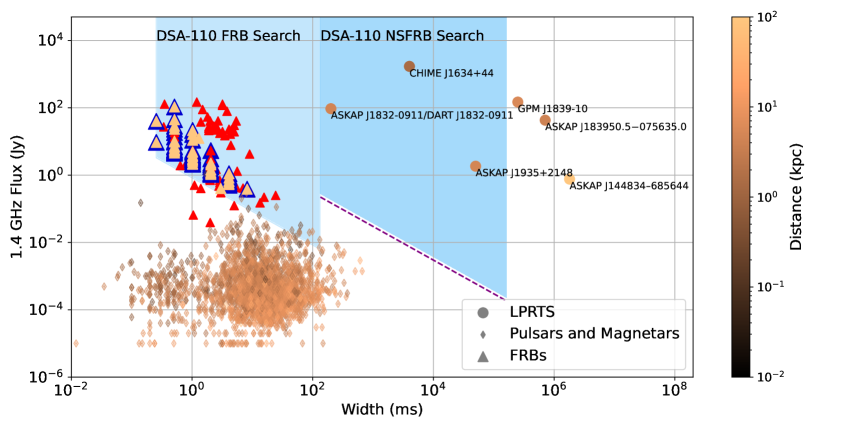
Figure 2: Pulse width and $6\sigma_{\rm srch}$ Fluence Sensitivity to $\Delta t=134$ ms Bursts of the DSA-110 FRB (light blue; $\sim 290\,$mJy ms) and NSFRB (dark blue hatched; $\sim 40\,$Jy ms) searches. For each search we assume the fluence threshold is fixed; thus the lower border indicates the corresponding flux density threshold $6\sigma_{\rm th}\Delta t/W$ where $W$ is the width. The purple dashed line shows the theoretical radiometer $6\sigma_{\rm th}$ sensitivity of the NSFRB survey. 1.4 GHz fluences and widths are shown for radio pulsars in the ATNF catalog (diamonds), FRBs from the literature (triangles), and LPRTs (circles). DSA-110 FRBs have dark blue outlines and show their detection pulse widths and S/N rather than refined estimates from baseband analysis. The colorbar indicates distance estimates in kpc (FRB luminosity distances are computed from host Galaxy redshifts; pulsar, magnetar, and LPRT distances are from parallaxes where available, and DM distance limits for the rest of the sample).

2.3 Candidate Post-Processing

When candidates are identified, the image, S/Ns for all pixels, widths, and DM trials, and times-of-arrival (TOAs) for all pixels, widths, and DM trials are saved to disk. The candidate timestamp is pushed to ETCD which is monitored by the post-processing system. Standard post-processing is limited to the 10 highest S/N candidates, under the assumption that each image will have at most one candidate. To identify the most likely candidate, we compare the candidates’ relative positions within the image to a simulated PSF. First, the PSF is thresholded at the 90^th percentile to make a binary mask, which is centered on each candidate in turn. This candidate is treated as the central PSF lobe, and any other candidates within the binary mask are identified as possible sidelobes. The weighted mean S/N is computed over the central and sidelobe candidate S/Ns. After repeating with each candidate, the maximum S/N is identified and its central lobe candidate’s width, DM, position, and TOA are taken as the final, most-likely candidate.

The second major post-processing stage is to apply a three-stage Convolutional Neural Network (CNN) classifier to the image to identify and rule out Radio Frequency Interference (RFI). The CNN is trained on a set of simulated point sources, simulated near- and far-field RFI, and field data sets of RFI and pulsar B0329+54 from NSFRB commissioning. The model consists of successive convolutional blocks with batch normalization, nonlinear activations, and max-pooling, followed by a small fully connected head with dropout; it is optimized with Adam using a binary cross-entropy loss. After applying the trained model to the 3D image cube (position, time, frequency), the network outputs a single logit for each candidate which, after a sigmoid activation, we interpret as the RFI probability (0 indicates likely astrophysical; 1 indicates likely RFI). Simulated injection tests and pulsar observations were used to verify classifier performance. Positively identified candidates are assigned a candidate name and metadata (RA, DEC, TOA, DM, width, and S/N) are saved to a json file. A candidate plot is saved and pushed as a Slack alert for human inspection; this shows the time and frequency averaged image, the S/N as a function of trial DM and width for the final candidate pixel, the dynamic spectrum from the final candidate pixel, and the de-dispersed time series from the final candidate pixel. Finally, a trigger is sent to the correlator nodes to dump voltage data for a $26.85$ second interval around the burst to disk for offline analysis and localization; voltage triggering is still being implemented.

3 Commissioning Injection and Pulsar Tests

NSFRB commissioning observations took place from February - October, 2025, including injection testing, pulsar observations, continuum source observations, and an offline Galactic Plane Survey (February - April). the latter two are discussed in Section 4.

3.1 False Positive and False Negative Injection Tests

A simulated injection pipeline was used to evaluate the search system’s false-negative rate; $\sim 200$ boxcar-shaped pulses with DMs between $0-4000\,$pc cm^-3, widths between $0.134-2.14\,$s, and S/N between $0-10\sigma$ were generated. The amplitude of each burst is scaled based on noise estimates from imaged fast visibility data. These were sent to the process server and searched, with the peak S/N candidate identified and saved. $\sim 2000$ noise realizations without pulses were similarly sent through the search pipeline to estimate the false-positive rate. Simultaneously minimizing as a function of S/N threshold, we estimate that a $6\sigma$ detection limit is optimal, yielding a $\sim 40\%$ false-negative rate and a $\sim 25\%$ false positive rate. A $6\sigma$ threshold was used for the Galactic Plane survey, while a more stringent $8.5\sigma$ has been adopted for the real-time pipeline to limit false positives while commissioning observations are completed.

3.2 Pulsar Observations

Observations of pulsar B0329+54 ($P=0.7145$ s, pulse profile FWHM$=6.6\,$ms, $S_{\rm 1.4\,GHz}=203$ mJy R. N. Manchester et al., 2005) were used to monitor the system’s sensitivity to transient pulsed emission which the NSFRB search is targeting. This pulsar is selected for its high pulse period ($\sim 5\times 134$ ms samples), long pulse duration, and high flux; it is the only northern sky pulsar with an expected single-pulse S/N$>5\sigma_{\rm srch}$. Single pulses (filling the remaining samples with Gaussian noise) from initial observations were used to train the CNN classifier. Later observations then properly detected and classified the pulsar. Figure 3 shows a candidate summary plot in which 5 pulses from B0329+54 were detected, demonstrating that the NSFRB search is sensitive to both single-pulsed and periodic emission. Note that pulsar B0329+54 has $DM=26.76410\,$pc cm^-3, but was detected at the DM=0 pc cm^-3 trial bin due to the coarse trial DM spacing. The next DM trial is $213.72\,$pc cm^-3.

The pulsar was observed during its transit for four consecutive days (MJDs 60947-60950; September 29 - October 2, 2025) to characterize the search sensitivity at each stage of the pipeline. Figure 4 summarizes the results; 1381 total pulses were recorded, with 658 detected above $3\sigma_{\rm srch}$. 8621 total candidates above the $8.5\sigma$ real-time threshold were detected; PSF-based reduction resulted in 1511 candidates; the classifier then allowed through 30 final candidates for which alerts were sent. No final candidates were identified on 2025-10-01; inspection of the data implies this was due to higher-than-average RFI contamination and an unfortunately timed system restart. The S/N distribution of pulses $>3\sigma$ peaks near $23\sigma$, consistent with the expected $19\sigma$. The B0329+54 observations demonstrate the pipeline has sensitivity aligned with theoretical predictions, can decimate a large number of triggers to a manageable number of candidates, and can properly classify real astrophysical single-pulses.

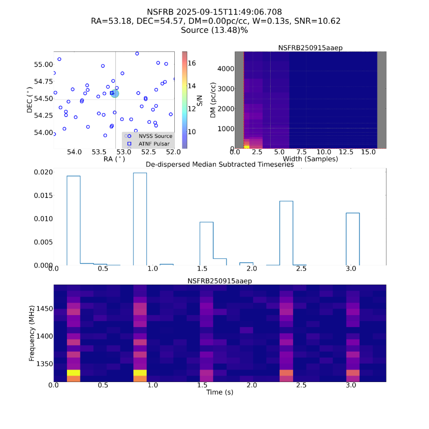
Figure 3: Example NSFRB candidate plot from detections of pulsar B0329+54. (top left) Position of the candidate (shaded circle) in reference to the pulsar’s catalogued position (open blue square) and other field NVSS continuum sources (open blue circles). The colorbar corresponds to the S/N. (top right) S/N as a function of search DM and pulse width. (middle) DM=0 0.134 ms-sampled time series of the peak candidate in arbitrary units. (bottom) Dynamic spectrum of the peak candidate with coarse 12 MHz channels. The title gives the UTC time of the first time sample, RA and declination after systematic error correction, detected DM, pulse width, and S/N, and the CNN classifier’s p-value.

Figure 4: Summary of Pulsar B0329+54 Monitoring Observations. (Top) The S/N of all pulses measured from predicted Times-of-Arrival (TOAs) are in blue. Initial candidates above the $8.5\sigma$ threshold are in grey, remaining candidates after PSF-based reduction are in black, and final candidates after classification are in red. (Bottom right) The S/N distribution of all single-pulses above $3\sigma$ are in blue, while ‘non-detections’ below $3\sigma$ are in grey. The median of the $>3\sigma$ distribution is indicated in red and compared to the predicted S/N in black. (Bottom left) The pulse profile (129 phase bins) formed as a histogram of TOAs weighted by detected S/N is shown in blue. Note that the folded profile is not phase connected between days, nor is it phase connected to past observations (e.g. A. Deller et al., 2019). The profile from the European Pulsar Network (EPN) database, scaled to the peak S/N of the detected profile, is shown in black (J. Seiradakis et al., 1995, https://psrweb.jb.man.ac.uk/epndb).

4 The DSA-110 NSFRB Galactic Plane Survey (DN-GPS)

4.1 Survey Strategy

The NSFRB instrument conducted an inaugural survey of the Galactic Plane (GP) from February 18 - April 23, 2025 (MJD 60724 - 60788). To accommodate the DSA-110’s lack of azimuthal drive, approximately hourly commands were issued to slew in declination to ‘track’ the plane, enabling roughly 20 degrees coverage in RA at each trial declination. This was repeated approximately daily starting 3 degrees further south each day, but slewing by the same hourly step-size. This strategy maximizes the time between slews (roughly hourly), extends vertical plane coverage, and limits instrumental strain by spacing its observation over a 12-day span. The 12-day pattern was repeated 6 discrete times to ensure complete coverage of the plane in the presence of maintenance or observer error. Figure 5 shows the DN-GPS coverage maps for each pass; the final survey covers $-3.5^{\circ}<b<5.7^{\circ}$ and $141^{\circ}<l<225^{\circ}$ in Galactic coordinates.

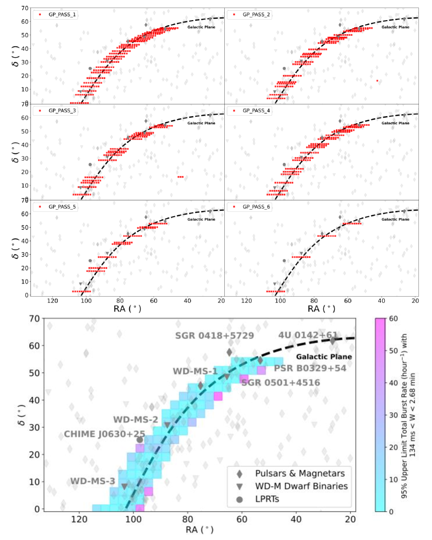
Figure 5: Coverage and Rate Limits for the DN-GPS pilot survey. (top) Each sub-plot shows one of 6 passes of the Galactic Plane (dashed black line). Center coordinates for each 3.35 s pointing are shown in red. The positions of known pulsars and magnetars are shown as diamonds; non-pulsar LPRTs detected to date are circles. A sample of White Dwarf-M Dwarf binaries from A. Rebassa-Mansergas et al. (2021) are shown as triangles. (bottom) 95% Poissonian burst rate upper limits are indicated by the colorbar for each $3^{\circ}\times 3^{\circ}$ grid region as discussed in Section 4. Sources of interest covered by the DN-GPS search region are labeled; of these, only B0329+54 is confidently detected.

4.2 Astrometric Calibration

Astrometric errors for candidates from the DN-GPS are estimated by comparing measured positions of sources from the Radio Fundamental Catalogue (RFC) to their milliarcsecond scale Very Long Baseline Interferometric (VLBI) localizations (L. Petrov & Y. Y. Kovalev, 2025). 16 RFC calibrators are selected as those that have 1.4 GHz flux measurements from the National Radio Astronomy Observatory (NRAO) VLA Sky Survey (NVSS; J. J. Condon et al., 1998) and fall within the DN-GPS field (see Figure 5). We form $175\times 175$ pixel images around each calibrator transit (between $1-30$ images, each averaged over 3.35 s) and use the casatools and Astropy.WCS modules to compute the RA and declination of each image pixel based on the current telescope pointing. Each image is fit with a 2D Gaussian around the main lobe of the RFC source to measure its position and align the images with each other, averaging over the full image set to maximize the signal-to-noise. This ‘alignment solution’ - the number of image pixels by which the source transits between each 3.35 s-fringestopped image - is also used to align images in the 0.67 s and 10.06 s search pipelines to correct small deviations from the expected transit due to the time and UV-grid resolution.

The final source position is measured from a 2D Gaussian fit of the full averaged image. We identify a statistically significant systematic position offset of $\epsilon_{\rm\alpha}=-1.77^{\prime}\pm 2^{\prime\prime}$, $\epsilon_{\rm\delta}=-1.15^{\prime}\pm 1^{\prime\prime}$ in RA and declination, respectively. After applying this correction, the remaining RMS position error is $\sigma_{\alpha}=12^{\prime\prime}$, $\sigma_{\delta}=7^{\prime\prime}$. Figure 6 (right) shows the final position offsets of the 16 calibrators with the $3\sigma$ position error circle.

4.3 Sensitivity and Flux Calibration

To estimate the flux sensitivity we convert the running standard deviation accumulated during the DN-GPS to flux units using 134 ms single-sample images of the 16 calibrators. The brightest source, J060351+215937 shown in Figure 7, is used to compute a conversion factor from arbitrary image pixel units to the NVSS catalog flux (2771.6 mJy). The same factor is applied to each calibrator observation as shown on the x-axis in Figure 6 (left). Applying this to an observing time-weighted average of the running standard deviation from each observing day, we estimate a sensitivity limit $\sigma_{\rm srch}\approx 50$ mJy, confirming that the calibrators follow an approximately linear relation down to the $3\sigma_{\rm srch}$ flux limit. Note the sensitivity ranged from $30-100\,$mJy depending on the observation date. NVSS and RFC sources are observed daily during real-time observations to continuously update flux estimates; we include real-time NVSS observations in Figure 6 which show that fainter sources’ measured flux flattens near $\sigma_{\rm srch}$ as expected.

As indicated in Figure 2, the measured $\sigma_{\rm srch}=50\,$mJy sensitivity exceeds the theoretical radiometer sensitivity estimate with approximately uniform $\mathcal{R}=-2$ image weights $\sigma_{\rm th}=40\,$mJy by roughly $1.3\times$. We attribute this in part to RFI excision. Both far- and near-field RFI have been observed, the former resulting from aircraft passing over the observatory and the latter from cellular networks transmitting near the center of the band. Near field RFI contributes to image-plane noise because it appears at all spatial scales rather than as a point source. The current pipeline adopts two visibility flagging criteria on the 1.5 MHz channels: (1) the mean visibility in the channel exceeds $5\times$ the running mean, (2) the peak median-subtracted visibility in the channel exceeds $10\times$ the running mean. These have proven effective in excising far-field RFI on a channel basis; however, near-field RFI may be leaking into adjacent channels, biasing the noise high in addition to the bandwidth reduction from channel flagging. Additional analysis is required to fully characterize RFI and devise techniques to recover sensitivity more robustly. Other potential effects that may lower sensitivity include primary beam attenuation, intrinsic flux calibrator variability, and poorly fit beamformer weights on a given day, which we do not investigate in detail here.

4.4 Results

No candidates were detected by the NSFRB pipeline from the DN-GPS data using a $6\sigma$ threshold. The data were re-searched multiple times with lower thresholds (as low as $2\sigma$) in order to inspect low S/N candidates in more detail, resulting in no marginal candidates.

As shown in Figure 5 (bottom), we partition the survey region into a grid of $3^{\circ}\times 3^{\circ}$ cells covering the total $\sim 774$ square degree survey area to estimate limits on the burst rate $R_{\rm 95}$ from the NSFRB non-detection. Note that we neglect primary beam effects for this calculation. To do this, we first assume that $R_{\rm 95}<T_{\rm obs}^{-1}$, where $T_{\rm obs}=5$ minutes is the duration of a single pointing dataset, approximately the time for which a target remains in the DSA-110 NSFRB image field. In this limit, we can use Poissonian statistics, adopting the weighted sum observing time from pointings that fall within each region, $T_{\rm tot,eff}$, using noise estimates from the date of observation ($\sim 40-60$ mJy) as inverse weights.

We estimate the upper limit on the total burst rate in each cell as $R_{\rm 95}=-T_{\rm tot,eff}^{-1}{\rm ln}(0.05)$ with 95% confidence. The results are shown in Figure 5; we find that $R_{\rm 95}$ ranges from $1-60$ hr^-1, with a weighted median $R_{\rm 95}<5.6$ hr^-1. The tightest constraints are at low Galactic latitudes $b$ and at declinations with the most complete coverage. For $|b|<0.25^{\circ}$, the maximum burst rate upper limit among $3^{\circ}\times 3^{\circ}$ cells is $R_{\rm 95}<7$ hr^-1 (or $<1$ hr^-1 per square degree).

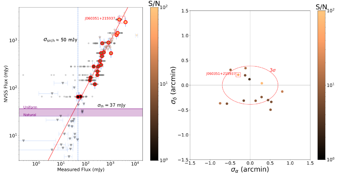
Figure 6: Flux and Astrometry Calibration Observations from the DSA-110 NSFRB Galactic Plane Survey (DN-GPS). (Left) Measured vs. NVSS catalogued flux for the 16 calibrators selected from DN-GPS data are shown as circles. Individual measurements are in grey, while the mean measurements have colorbar equal to the observed signal-to-noise. Additional calibrator observations from the real-time pipeline are shown as triangles. The red line shows the conversion curve constrained from the brightest source, J060351+215937, and the sensitivity limit $\sigma_{\rm srch}$ is shown in blue. The range of theoretical sensitivity limits from natural to approximately uniform $\mathcal{R}=-2$ imaging weights is shown in purple. (Middle) Measured position errors of the 16 calibrators, after subtracting the mean systematic offsets $\epsilon_{\rm\alpha}=-1.77^{\prime}\pm 2^{\prime\prime}$, $\epsilon_{\rm\delta}=-1.15^{\prime}\pm 1^{\prime\prime}$ from RFC positions, are shown as circles with colorbar equal to the observed signal-to-noise. The $3\sigma$ error ellipse ($72^{\prime\prime}\times 42^{\prime\prime}$) is outlined in red.

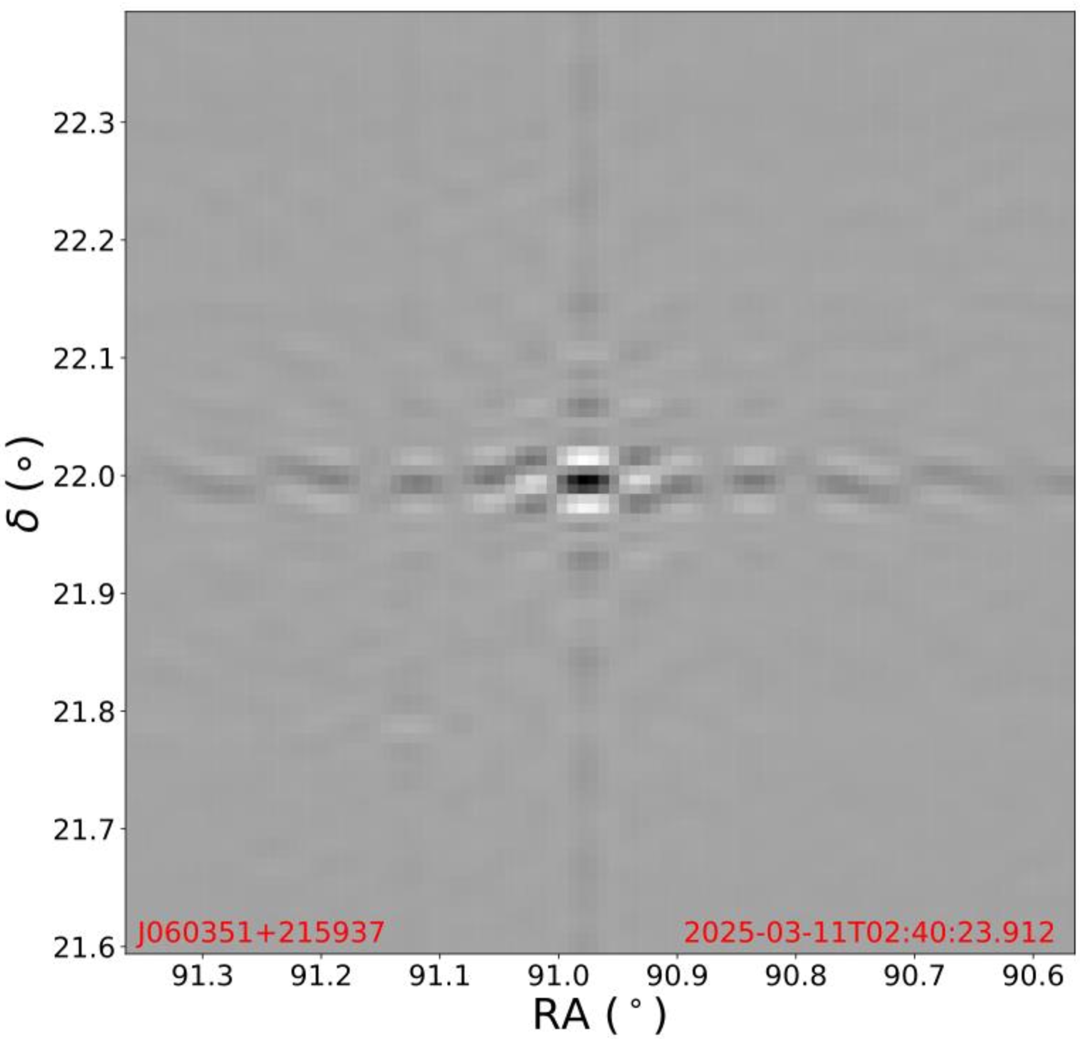
Figure 7: A Time- (3.35 s) and Frequency- (187.5 MHz) Averaged Dirty Image of Calibrator J060351+215937 where PSF and central sidelobes are visible. Dark regions are positive and light regions are negative in arbitrary units. J060351+215937 was the brightest calibrator observed during the DSA-110 NSFRB Galactic Plane Survey (DN-GPS) and was used to estimate the flux curve shown in Figure 6.

5 Discussion

While no candidates are detected, this is the first targeted search for LPRTs at 1.4 GHz, and the burst rate limit can be used to constrain models for LPRT emission. In this section, we contrast the detectability of two predominant models: the isolated neutron star model from A. Cooper & Z. Wadiasingh (2024) and the White Dwarf-M Dwarf model from Y. Qu & B. Zhang (2025).

5.1 Relevant Noise Estimates for Long and Short Periods

For this discussion, we partition the analysis at pulse period $P=T_{\rm obs}=5$ minutes; for $P<T_{\rm obs}$, we assume that the LPRT is always “on”, thus, if the flux exceeds the instantaneous noise level $6\sigma_{\rm srch}$ in any $5-$minute observation, it will be detected. Therefore, for each $3^{\circ}\times 3^{\circ}$ grid cell, we take the minimum noise estimate among each contributing observing day as the relevant detection limit. The median among all grid cells is then $\sigma_{\rm srch,P<5\,min}\approx 40\,$mJy.

For $P>T_{\rm obs}$, although the source is always “on”, the long period allows us to treat it as a Poissonian process. Just as the effective rate limit adopts a weighted sum observing time, $T_{\rm tot,eff}$, for each grid cell, we use the median noise estimate among each contributing observing day as the relevant detection limit. The median among all grid cells is then $\sigma_{\rm srch,P>5\,min}\approx 50\,$mJy. In the next section we use $\sigma_{\rm srch}=\sigma_{\rm srch,P<5\,min}$ and $\sigma_{\rm srch}=\sigma_{\rm srch,P>5\,min}$ for $P<5$ minutes and $P>5$  minutes unless otherwise stated. The distinction is indicated in Figure 8 by a labeled vertical grey line at $P=5\,$minutes.

5.2 Constraints on the White Dwarf-M Dwarf Binary and Neutron Star Models

In the A. Cooper & Z. Wadiasingh (2024) neutron star model, plastic motion of the crust of a post-deathline magnetar induces twist in the magnetic field, storing magnetic energy. This energy is released over $\sim$days, driving pair-plasma creation of charged particles. The resulting charges accelerate in a vacuum gap potential and coherently radiate via curvature radiation or inverse-Compton scattering. The maximum dissipation luminosity, which notably excludes the efficiency of pair-creation (e.g. P. N. Arendt Jr & J. A. Eilek, 2002), is below:

$$L_{\rm diss,NS}\approx\frac{v_{\rm p}B_{S}^{2}A_{\rm fp}R_{NS}}{cP\sin^{2}(\theta_{\rm fp})}$$ (2)

where $v_{\rm p}\lesssim 10^{6}\,$cm yr^-1 is the velocity of plastic flow, $B_{S}\approx 10^{15}$ G is the surface magnetic field strength, $A_{\rm fp}\approx 10\,$km is the size of the crust ‘footprint” undergoing plastic motion, and $\theta_{\rm fp}$ is the co-latitude of the footprint. By asserting that $L_{\rm diss,NS}>6\sigma_{\rm srch}d^{2}{\rm BW}$ for an LPRT at distance $d$ within this model, and using the characteristic $B_{S}\gtrsim(3.2\times 10^{19}\,G)\sqrt{P\dot{P}/2}$, we can solve for the maximum distance $d_{\rm max,NS}(P,\dot{P})$ to which the DN-GPS could detect the LPRT. Figure 8 (top) shows this result with $v_{\rm pl}=10^{4}$ cm yr^-1; we see that for $\dot{P}>10^{-14}$ and $P<R^{-1}_{\rm 95}=10.7$ min the search is complete to only 1 kpc. To the edge of the galaxy, approximately $30\,$kpc, the search is only sensitive to $\dot{P}>10^{-11}$. Based on the $\dot{P}$ range of detected LPRTs with $P<R^{-1}_{\rm 95}=10.7$ min, this indicates that the search is not sensitive to magnetar-LPRTs beyond $1\,$kpc. In addition, A. Cooper & Z. Wadiasingh (2024) indicate that the plastic flow velocity can reasonably range from $1<v_{\rm pl}<10^{6}$ cm yr^-1, which is proportional to $L_{\rm diss,NS}$ and can significantly alter the horizon distance. Therefore, the search is not complete for magnetar-LPRT objects; we conclude that a population of ultra-long period magnetars may still be present within the Galactic Plane despite our non-detection.

In the Y. Qu & B. Zhang (2025) White Dwarf-M Dwarf binary model, the companion star orbits within the White Dwarf’s magnetosphere, creating a voltage drop between the two stars via the unipolar inductor effect (Faraday disk). As charge flows between the stars due to the potential drop they create an electrical current, and the magnetosphere dissipates power via Ohmic heating, driving pair creation. Pair charges then radiate via the relativistic electron cyclotron maser mechanism. We adjust the derivation from Y. Qu & B. Zhang (2025) to allow non-zero spin-down $\dot{P}$; a brief derivation is provided in Appendix A, obtaining the following dissipation luminosity:

$$L_{\rm diss,WD}=\frac{4\pi}{c}\biggl(\frac{B_{\rm WD}R_{\rm WD}^{3}R_{c}\zeta(4\pi^{2})^{2/3}}{(G(M_{\rm WD}+M_{c}))^{2/3}}\biggr)^{2}(\frac{1}{P^{14/3}}-\frac{14}{3}\frac{\dot{P}\tau}{P^{17/3}})$$ (3)

where $B_{\rm WD}\approx 10^{6}$ G is the surface magnetic field strength of the White Dwarf star, $M_{WD}$ and $M_{c}$ are the stars’ masses, $R_{WD}$ and $R_{c}$ are the stars’ radii, and $\tau\lesssim 1$ Gyr is the timespan over which the White Dwarf radiates. Here we normalize $\zeta\equiv|P^{-1}-P_{\rm rot}^{-1}|P=1$ where $P$ is the orbital period and $P_{\rm rot}$ is the White Dwarf’s rotation period; we assume $\tau\approx\tau_{\rm age}=1\,$Gyr, the typical White Dwarf age, as an upper limit, which will yield a more conservative range of $\dot{P}$ values (see Appendix A for justification of these assumptions). We apply the same detection condition, $L_{\rm diss,WD}>6\sigma_{\rm srch}d^{2}{\rm BW}$, and the resulting $d_{\rm max,WD}(P,\dot{P})$ is shown in Figure 8 (bottom). In this case, the DN-GPS is sensitive to WD-binary-LPRT objects within $d\lesssim 30\,$kpc for $P\lesssim 70\,$s. By this model, our non-detection determines that across 738 square degrees ($\sim 95\%$) of the survey region (excluding only 4 grid-points on the outskirts with $R_{\rm 95}^{-1}<70$ s) there are no WD-binary-LPRTs with $S_{\rm 1.4\,GHz}>6\sigma_{\rm srch,P<5\,min}\approx 250$ mJy and $10\lesssim P\lesssim 70$ s. While only a fraction of the allowed $P-\dot{P}$ parameter space is constrained, our results motivate further discussion of both the White Dwarf-M Dwarf binary and magnetar LPRT models.

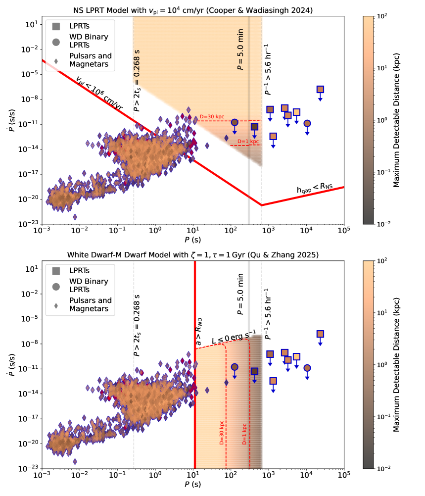
Figure 8: $P-\dot{P}$ Constraints from the DN-GPS Survey Using a Neutron Star Model (top; A. Cooper & Z. Wadiasingh, 2024) and a White Dwarf Model (bottom; Y. Qu & B. Zhang, 2025). In each plot the thick red lines bound the allowed emission ranges for each model. Vertical grey lines indicate hard limits from the DN-GPS search due to the sampling time and Poissonian burst rate. Pulsars (diamonds), WD binary LPRTs (squares) and all other LPRTs (circles) are colored with their distance estimates, while those without distances are in red. The colorbar also highlights the maximum detectable distance ($d_{\rm max}(P,\dot{P})$) for each model (see Section 4) given the DN-GPS $6\sigma_{\rm srch,P<5\,min}\approx 250$ mJy and $6\sigma_{\rm srch,P>5\,min}\approx 300$ mJy detection limits for $P<5\,$min and $P>5$ min, respectively. Red dashed lines are contours of constant $d_{\rm max}(P,\dot{P})$).

6 Conclusion

We have developed and commissioned the DSA-110 NSFRB instrument, a GPU-accelerated image-plane single-pulse search sensitive to bright LPRTs with pulse widths between $134\,$ms$-160.8\,$s. Initial continuum source observations have been largely successful and the pulsar B0329+54 is routinely detected. The inaugural DN-GPS survey recovered no candidates, placing limited constraints on the White Dwarf-M Dwarf binary model. The real-time NSFRB search is online in drift-scan mode, adopting hourly source injections, daily calibrator and pulsar observations, and weekly construction of classifier re-training sets from false-positive detections for system health evaluation. Future work will explore triggered periodicity searching, further expansion of the pulse width range, and more DN-GPS-like surveys of the Galactic Plane, star-forming regions, and globular clusters.

7 Data Availability

The NSFRB code is publicly available at https://github.com/dsa110/dsa110-nsfrb.

Appendix A Derivation of Time-dependent Dissipation Luminosity for the White Dwarf Model

In this appendix, we derive equation 3 incorporating time dependence. Starting from Equation 9 in Y. Qu & B. Zhang (2025), the total voltage when the White Dwarf and M-dwarf are at a separation $a(t)$ is given by:

$$\Phi(t)=\frac{2\mu R_{c}}{ca(t)^{2}}\zeta\Omega(t)$$ (A1)

where we introduce time-dependence in the orbital period $P=2\pi/\Omega$ and orbital separation $a$, and define $\zeta\equiv|\Omega-\Omega_{\rm rot}|/\Omega\sim$ constant where $\Omega_{\rm rot}$ is the rotational period of the White Dwarf. Recall the magnetic dipole moment $\mu\approx B_{\rm WD}R_{\rm WD}^{3}$, and Kepler’s law $a(t)^{3}=G(M_{\rm WD}+M_{\rm c})P(t)^{2}/(4\pi)$. Plugging these in for $\mu$ and $a(t)$, respectively:

$$\Phi(t)=\frac{2B_{\rm WD}R_{\rm WD}^{3}R_{c}\zeta(4\pi^{2})^{2/3}}{c(G(M_{\rm WD}+M_{c})P^{2}(t))^{2/3}}\frac{2\pi}{P(t)}$$ (A2)

$$\Phi(t)=\frac{2B_{\rm WD}R_{\rm WD}^{3}R_{c}\zeta(4\pi^{2})^{2/3}}{c(G(M_{\rm WD}+M_{c}))^{2/3}}\frac{2\pi}{P^{7/3}(t)}=KP(t)^{-7/3},\quad K\equiv\frac{4\pi B_{\rm WD}R_{\rm WD}^{3}R_{c}\zeta(4\pi^{2})^{2/3}}{c(G(M_{\rm WD}+M_{c}))^{2/3}}$$ (A3)

Let the resistance of the magnetosphere be $R_{\rm mag}=4\pi/c$. The ohmic dissipation power is then written as:

$$\dot{E}_{\rm diss}(t)=\frac{c}{4\pi}K^{2}P(t)^{-14/3}$$ (A4)

If we assume the orbital period evolves slowly as $P(t)=P_{0}+\dot{P}t$ to first order, we can write the dissipation power as:

$$\dot{E}_{\rm diss}(t)=\frac{c}{4\pi}K^{2}(P_{0}+\dot{P}t)^{-14/3}$$ (A5)

$$\dot{E}_{\rm diss}(t)=\frac{c}{4\pi}K^{2}P_{0}^{-14/3}(1+\frac{\dot{P}}{P_{0}}t)^{-14/3}$$ (A6)

If $\dot{P}t\ll P_{0}$, we can expand this to first order:

$$\dot{E}_{\rm diss}(t)=\frac{c}{4\pi}K^{2}P_{0}^{-14/3}(1-\frac{14}{3}\frac{\dot{P}}{P_{0}}t)$$ (A7)

Then, substituting in for $K$ and evaluating at the timespan over which the White Dwarf radiates $t=\tau$, we obtain equation 3:

$$L_{\rm diss,WD}\equiv\dot{E}_{\rm diss}(\tau)=\frac{4\pi}{c}\biggl(\frac{B_{\rm WD}R_{\rm WD}^{3}R_{c}\zeta(4\pi^{2})^{2/3}}{(G(M_{\rm WD}+M_{c}))^{2/3}}\biggr)^{2}(\frac{1}{P_{0}^{14/3}}-\frac{14}{3}\frac{\dot{P}\tau}{P_{0}^{17/3}})$$ (A8)

Note that in general, we expect $\tau\ll\tau_{\rm age}\sim 1$ Gyr; for example, GPM J1839-10 was detected in archival data over the course of 36 years. Using its upper limit $\dot{P}<3.6\times 10^{-13}$ and measured $P=31482.4\,$s, we find $\dot{P}\tau/P\sim 10^{-8}$ for $\tau=36\,$years (C. Horváth et al., 2025; Y. Men et al., 2025). Even for $\tau=1\,$Gyr, we have $\dot{P}\tau/P\sim 10^{-1}$. Therefore we conclude the solution is valid in general for the LPRT case. Note also that $\zeta$ can vary over a wide range ($\zeta\sim 22$ for GPM J1839-10), but we normalize it to unity for this discussion as in Y. Qu & B. Zhang (2025).

References

- P. N. Arendt Jr & J. A. Eilek (2002) Arendt Jr, P. N., & Eilek, J. A. 2002, \bibinfotitlePair creation in the pulsar magnetosphere, The Astrophysical Journal, 581, 451
- P. Beniamini et al. (2023) Beniamini, P., Wadiasingh, Z., Hare, J., et al. 2023, \bibinfotitleEvidence for an abundant old population of Galactic ultra-long period magnetars and implications for fast radio bursts, Monthly Notices of the Royal Astronomical Society, 520, 1872
- P. Beniamini et al. (2020) Beniamini, P., Wadiasingh, Z., & Metzger, B. D. 2020, \bibinfotitlePeriodicity in recurrent fast radio bursts and the origin of ultralong period magnetars, Monthly Notices of the Royal Astronomical Society, 496, 3390
- D. S. Briggs (1995) Briggs, D. S. 1995, \bibinfotitleHigh fidelity deconvolution of moderately resolved sources, Ph. D. Thesis
- G. Bruni et al. (2025) Bruni, G., Piro, L., Yang, Y.-P., et al. 2025, \bibinfotitleDiscovery of a persistent radio source associated with FRB 20240114A, Astronomy & Astrophysics, 695, L12
- M. Caleb et al. (2022a) Caleb, M., Rajwade, K., Desvignes, G., et al. 2022a, \bibinfotitleRadio and X-ray observations of giant pulses from XTE J1810- 197, Monthly Notices of the Royal Astronomical Society, 510, 1996
- M. Caleb et al. (2022b) Caleb, M., Heywood, I., Rajwade, K., et al. 2022b, \bibinfotitleDiscovery of a radio-emitting neutron star with an ultra-long spin period of 76 s, Nature Astronomy, 6, 828
- M. Caleb et al. (2024) Caleb, M., Lenc, E., Kaplan, D., et al. 2024, \bibinfotitleAn emission-state-switching radio transient with a 54-minute period, Nature Astronomy, 8, 1159
- E. Carli et al. (2024) Carli, E., Levin, L., Stappers, B., et al. 2024, \bibinfotitleThe TRAPUM Small Magellanic Cloud pulsar survey with MeerKAT–I. Discovery of seven new pulsars and two Pulsar Wind Nebula associations, Monthly Notices of the Royal Astronomical Society, 531, 2835
- A. Chrimes et al. (2022) Chrimes, A., Levan, A. J., Fruchter, A., et al. 2022, \bibinfotitleNew candidates for magnetar counterparts from a deep search with the Hubble Space Telescope, Monthly Notices of the Royal Astronomical Society, 512, 6093
- J. J. Condon et al. (1998) Condon, J. J., Cotton, W., Greisen, E., et al. 1998, \bibinfotitleThe NRAO VLA sky survey, The Astronomical Journal, 115, 1693
- A. Cooper & Z. Wadiasingh (2024) Cooper, A., & Wadiasingh, Z. 2024, \bibinfotitleBeyond the rotational deathline: radio emission from ultra-long period magnetars, Monthly Notices of the Royal Astronomical Society, 533, 2133
- W. Cotton et al. (2024) Cotton, W., Filipović, M., Camilo, F., et al. 2024, \bibinfotitleThe MeerKAT 1.3 GHz Survey of the Small Magellanic Cloud, Monthly Notices of the Royal Astronomical Society, 529, 2443
- I. de Ruiter et al. (2025) de Ruiter, I., Rajwade, K., Bassa, C., et al. 2025, \bibinfotitleSporadic radio pulses from a white dwarf binary at the orbital period, Nature Astronomy, 1
- A. Deller et al. (2019) Deller, A., Goss, W., Brisken, W., et al. 2019, \bibinfotitleMicroarcsecond VLBI pulsar astrometry with PSR II. Parallax distances for 57 pulsars, The Astrophysical Journal, 875, 100
- D. Dobie et al. (2024) Dobie, D., Zic, A., Oswald, L. S., et al. 2024, \bibinfotitleA two-minute burst of highly polarized radio emission originating from low Galactic latitude, Monthly Notices of the Royal Astronomical Society, 535, 909
- F. A. Dong et al. (2023) Dong, F. A., Crowter, K., Meyers, B. W., et al. 2023, \bibinfotitleThe second set of pulsar discoveries by CHIME/FRB/Pulsar: 14 rotating radio transients and 7 pulsars, Monthly Notices of the Royal Astronomical Society, 524, 5132
- F. A. Dong et al. (2025a) Dong, F. A., Clarke, T. E., Curtin, A., et al. 2025a, \bibinfotitleCHIME/Fast Radio Burst/Pulsar Discovery of a Nearby Long-period Radio Transient with a Timing Glitch, The Astrophysical Journal Letters, 990, L49
- F. A. Dong et al. (2025b) Dong, F. A., Shin, K., Law, C., et al. 2025b, \bibinfotitleCHIME/Fast Radio Burst Discovery of an Unusual Circularly Polarized Long-period Radio Transient with an Accelerating Spin Period, The Astrophysical Journal Letters, 988, L29
- B. M. Gaensler et al. (2005) Gaensler, B. M., Kouveliotou, C., Gelfand, J., et al. 2005, \bibinfotitleAn expanding radio nebula produced by a giant flare from the magnetar SGR 1806–20, Nature, 434, 1104
- C. Gheller et al. (2023) Gheller, C., Taffoni, G., & Goz, D. 2023, \bibinfotitleHigh performance w-stacking for imaging radio astronomy data: a parallel and accelerated solution, RAS Techniques and Instruments, 2, 91
- J. Han et al. (2021) Han, J., Wang, C., Wang, P., et al. 2021, \bibinfotitleThe FAST Galactic Plane Pulsar Snapshot survey: I. Project design and pulsar discoveries⋆, Research in Astronomy and Astrophysics, 21, 107
- C. Horváth et al. (2025) Horváth, C., Rea, N., Hurley-Walker, N., et al. 2025, \bibinfotitleA unified model for long-period radio transients and white dwarf binary pulsars, arXiv preprint arXiv:2507.15352
- N. Hurley-Walker et al. (2022) Hurley-Walker, N., Zhang, X., Bahramian, A., et al. 2022, \bibinfotitleA radio transient with unusually slow periodic emission, Nature, 601, 526
- N. Hurley-Walker et al. (2023) Hurley-Walker, N., Rea, N., McSweeney, S., et al. 2023, \bibinfotitleA long-period radio transient active for three decades, Nature, 619, 487
- N. Hurley-Walker et al. (2024) Hurley-Walker, N., McSweeney, S., Bahramian, A., et al. 2024, \bibinfotitleA 2.9 hr Periodic Radio Transient with an Optical Counterpart, The Astrophysical Journal Letters, 976, L21
- S. D. Hyman et al. (2005) Hyman, S. D., Lazio, T. J. W., Kassim, N. E., et al. 2005, \bibinfotitleA powerful bursting radio source towards the Galactic Centre, nature, 434, 50
- N. Kosogorov et al. (2025) Kosogorov, N., Hallinan, G., Law, C., et al. 2025, \bibinfotitleImplementing Continuous All-sky Monitoring with the OVRO-LWA to Identify Prompt and Precursor Counterparts of Gravitational Wave Events, ApJ, 985, 265, doi: 10.3847/1538-4357/add014
- M. Kramer et al. (2024) Kramer, M., Liu, K., Desvignes, G., Karuppusamy, R., & Stappers, B. W. 2024, \bibinfotitleQuasi-periodic sub-pulse structure as a unifying feature for radio-emitting neutron stars, Nature Astronomy, 8, 230
- C. Law et al. (2018) Law, C., Bower, G., Burke-Spolaor, S., et al. 2018, \bibinfotitlerealfast: real-time, commensal fast transient surveys with the Very Large Array, The Astrophysical Journal Supplement Series, 236, 8
- C. J. Law et al. (2024) Law, C. J., Sharma, K., Ravi, V., et al. 2024, \bibinfotitleDeep synoptic array science: first FRB and host galaxy catalog, The Astrophysical Journal, 967, 29
- Y. Lee et al. (2025) Lee, Y., Caleb, M., Murphy, T., et al. 2025, \bibinfotitleThe emission of interpulses by a 6.45-h-period coherent radio transient, Nature Astronomy, 9, 393
- D. Li et al. (2024) Li, D., Yuan, M., Wu, L., et al. 2024, \bibinfotitleA 44-minute periodic radio transient in a supernova remnant, arXiv preprint arXiv:2411.15739
- Y. Li et al. (2025) Li, Y., Wang, L., Qian, L., et al. 2025, \bibinfotitleSearching for pulsars in Globular Clusters with the Fast Fold Algorithm and a new pulsar discovered in M13, arXiv preprint arXiv:2505.05021
- R. N. Manchester et al. (2005) Manchester, R. N., Hobbs, G. B., Teoh, A., & Hobbs, M. 2005, \bibinfotitleThe Australia telescope national facility pulsar catalogue, The Astronomical Journal, 129, 1993
- R. N. Manchester et al. (2001) Manchester, R. N., Lyne, A. G., Camilo, F., et al. 2001, \bibinfotitleThe Parkes multi-beam pulsar survey–I. Observing and data analysis systems, discovery and timing of 100 pulsars, Monthly Notices of the Royal Astronomical Society, 328, 17
- T. Marsh et al. (2016) Marsh, T., Gänsicke, B., Hümmerich, S., et al. 2016, \bibinfotitleA radio-pulsing white dwarf binary star, Nature, 537, 374
- S. J. McSweeney et al. (2025) McSweeney, S. J., Hurley-Walker, N., Horváth, C., et al. 2025, \bibinfotitleA new long-period radio transient: discovery of pulses repeating every 1.16 h from ASKAP J175534. 9- 252749.1, Monthly Notices of the Royal Astronomical Society, 542, 203
- Y. Men et al. (2025) Men, Y., McSweeney, S., Hurley-Walker, N., Barr, E., & Stappers, B. 2025, \bibinfotitleA highly magnetized long-period radio transient exhibiting unusual emission features, Science Advances, 11, eadp6351
- D. Mitra et al. (2023) Mitra, D., Melikidze, G. I., & Basu, R. 2023, \bibinfotitleMeterwavelength Single Pulse Polarimetric Emission Survey. VI. Toward Understanding the Phenomenon of Pulsar Polarization in Partially Screened Vacuum Gap Model, The Astrophysical Journal, 952, 151
- A. Paszke et al. (2019) Paszke, A., Gross, S., Massa, F., et al. 2019, \bibinfotitlePyTorch: An Imperative Style, High-Performance Deep Learning Library, arXiv e-prints, arXiv:1912.01703, doi: 10.48550/arXiv.1912.01703
- L. Petrov & Y. Y. Kovalev (2025) Petrov, L., & Kovalev, Y. Y. 2025, \bibinfotitleThe Radio Fundamental Catalog. I. Astrometry, The Astrophysical Journal Supplement Series, 276, 38
- Y. Qu & B. Zhang (2025) Qu, Y., & Zhang, B. 2025, \bibinfotitleMagnetic Interactions in White Dwarf Binaries as Mechanism for Long-period Radio Transients, The Astrophysical Journal, 981, 34
- V. Radhakrishnan & D. J. Cooke (1969) Radhakrishnan, V., & Cooke, D. J. 1969, \bibinfotitleMagnetic Poles and the Polarization Structure of Pulsar Radiation, Astrophys. Lett., 3, 225
- S. M. Ransom (2001) Ransom, S. M. 2001, New search techniques for binary pulsars (Harvard University)
- V. Ravi et al. (2023) Ravi, V., Catha, M., Chen, G., et al. 2023, \bibinfotitleDeep synoptic array science: discovery of the host galaxy of FRB 20220912A, The Astrophysical Journal Letters, 949, L3
- A. Rebassa-Mansergas et al. (2021) Rebassa-Mansergas, A., Solano, E., Jiménez-Esteban, F. M., et al. 2021, \bibinfotitleWhite dwarf-main-sequence binaries from Gaia EDR3: the unresolved 100 pc volume-limited sample, MNRAS, 506, 5201, doi: 10.1093/mnras/stab2039
- J. Seiradakis et al. (1995) Seiradakis, J., Gil, J., Graham, D., et al. 1995, \bibinfotitlePulsar profiles at high frequencies. I. The data., Astronomy and Astrophysics Supplement, v. 111, p. 205, 111, 205
- K. Sharma et al. (2024) Sharma, K., Ravi, V., Connor, L., et al. 2024, \bibinfotitlePreferential occurrence of fast radio bursts in massive star-forming galaxies, Nature, 635, 61
- S. Singh et al. (2022) Singh, S., Roy, J., Panda, U., et al. 2022, \bibinfotitleThe GMRT High Resolution Southern Sky Survey for Pulsars and Transients. III. Searching for Long-period Pulsars, The Astrophysical Journal, 934, 138
- C. Tan et al. (2018) Tan, C., Bassa, C., Cooper, S., et al. 2018, \bibinfotitleLOFAR Discovery of a 23.5 s Radio Pulsar, The Astrophysical Journal, 866, 54
- A. R. Thompson et al. (2017) Thompson, A. R., Moran, J. M., & Swenson, G. W. 2017, Interferometry and synthesis in radio astronomy (Springer Nature)
- E. van der Wateren et al. (2023) van der Wateren, E., Bassa, C. G., Cooper, S., et al. 2023, \bibinfotitleThe LOFAR Tied-Array All-Sky Survey: Timing of 35 radio pulsars and an overview of the properties of the LOFAR pulsar discoveries, Astronomy & Astrophysics, 669, A160
- W. van Straten et al. (2021) van Straten, W., Jameson, A., & Osłowski, S. 2021, \bibinfotitlePSRDADA: Distributed acquisition and data analysis for radio astronomy, Astrophysics Source Code Library, ascl
- Z. Wang et al. (2025a) Wang, Z., Rea, N., Bao, T., et al. 2025a, \bibinfotitleDetection of X-ray emission from a bright long-period radio transient, Nature, 1
- Z. Wang et al. (2025b) Wang, Z., Bannister, K., Gupta, V., et al. 2025b, \bibinfotitleThe CRAFT coherent (CRACO) upgrade I: System description and results of the 110-ms radio transient pilot survey, Publications of the Astronomical Society of Australia, 42, e005