Hierarchical summaries for primordial non-Gaussianities

The advent of Stage IV galaxy redshift surveys such as DESI and Euclid marks the beginning of an era of precision cosmology, with one key objective being the detection of primordial non-Gaussianities (PNG), potential signatures of inflationary physics. In particular, constraining the amplitude of local-type PNG, parameterised by $f_{\rm NL}$, with $\sigma_{f_{\rm NL}}\sim 1$, would provide a critical test of single versus multi-field inflation scenarios. While current large-scale structure and cosmic microwave background analyses have achieved $\sigma_{f_{\rm NL}}\sim 5$–$9$, further improvements demand novel data compression strategies. We propose a hybrid estimator that hierarchically combines standard $2$-point and $3$-point statistics with a field-level neural summary, motivated by recent theoretical work that shows that such a combination is nearly optimal, disentangling primordial from late-time non-Gaussianity. We employ PatchNet, a convolutional neural network that extracts small-scale information from sub-volumes (patches) of the halo number density field while large-scale information is retained via the power spectrum and bispectrum. Using Quijote-PNG simulations, we evaluate the Fisher information of this combined estimator across various redshifts, halo mass cuts, and scale cuts. Our results demonstrate that the inclusion of patch-based field-level compression always enhances constraints on $f_{\rm NL}$, reaching gains of $30$–$45\%$ at low $k_{\rm max}$ ($\sim 0.1\,h\,\text{Mpc}^{-1}$), and capturing information beyond the bispectrum. This approach offers a computationally efficient and scalable pathway to tighten the PNG constraints from forthcoming survey data.

1 Introduction

With the results and observations from stage IV surveys, such as the data release 1 of the Dark Energy Spectroscopic Instrument (DESI; DESI Collaboration et al., 2016; Adame et al., 2025) and the first observations by Euclid (Euclid Collaboration: Mellier et al., 2025), we have entered the era of precision large-scale structure (LSS) cosmology. The key objective of the new generation surveys, such as DESI and Euclid, but also SPHEREx (Crill et al., 2020), and the Vera C. Rubin Legacy Survey of Space and Time (LSST; LSST Science Collaboration et al., 2009), is to stress test the standard $\Lambda$CDM cosmological model, both at late times, measuring the dark energy equation of state; and at early times, detecting primordial features that would be smoking guns of inflation. In particular, inflationary models predict small deviations from Gaussianity in the primordial density distribution, called primordial non-Gaussianities (PNG), the footprint of which we should be able to observe in the late-time distribution of galaxies.

Different inflation models produce different types of PNG, see Baumann (2011) for a review. In this work, we are interested in the PNG of local type, which we parametrise with $f_{\rm NL}$. This parameter controls the amplitude of the non-linear relation between a mean-zero Gaussian field, $\varphi$, and the primordial gravitational potential, $\Phi_{P}=\varphi+f_{\rm NL}(\varphi^{2}-\langle\varphi^{2}\rangle)$. We know that local PNG should be very close to zero in the case of single-field inflation (Maldacena, 2003; Creminelli & Zaldarriaga, 2004; Cabass et al., 2017), while $f_{\rm NL}\sim\mathcal{O}(1)$ for multi-field inflation models (Senatore & Zaldarriaga, 2012; Alvarez et al., 2014). Therefore, a detection or non-detection of local PNG with $\sigma_{f_{\rm NL}}\sim 1$ would rule out single-field inflation or constraint multi-field models, respectively. For this reason, intensive efforts took place in the cosmological community to measure and improve our constraining power over this observable using different probes.

Currently, the most stringent constraints for $f_{\rm NL}$ come from the measurements of the $3$-point function of the cosmic microwave background (CMB) by Planck and are consistent with zero with $\sigma_{f_{\rm NL}}\sim 5$ (Planck Collaboration et al., 2020). We expect the new generation of CMB surveys to tighten these bounds by a factor of $2$, but not to reach $\sigma_{f_{\rm NL}}\sim 1$ (Abazajian et al., 2016). On the other hand, local PNG affect the late-time LSS both at the $2$- and $3$-point function level, which, in Fourier space, correspond to the power spectrum and the bispectrum (Dalal et al., 2008; Slosar et al., 2008; Desjacques & Seljak, 2010). The most stringent bounds from LSS measurements come from the power spectrum analysis of the first data release of DESI and reads $\sigma_{f_{\rm NL}}\sim 9$ (Chaussidon et al., 2025), which corresponds to a $40\%$ improvement over the previous power spectrum-based measurement that used the quasar sample of data release 16 of the extended Baryon Oscillation Spectroscopic Survey (Cagliari et al., 2024) and over $50\%$ improvement with respect to previous measurements based on power spectrum and bispectrum (e.g., D’Amico et al., 2025; Cabass et al., 2022). This shows a first glimpse of the constraining power of stage IV surveys. These results will improve even more when the complete surveys become available.

At the same time as gathering new data, we may attempt to improve our constraints on $f_{\rm NL}$, or other cosmological parameters, by devising new estimators that retain more information than the standard approach. For example, the authors of Castorina et al. (2019) computed the optimal quadratic estimator to measure the cosmological $f_{\rm NL}$ signal from the LSS power spectrum multipoles. Additionally, many works combine the power spectrum and the bispectrum (Cagliari et al., 2025) and utilise effective field theory (EFT; see Cabass et al., 2023, for a review) to extend the scale range we can probe with these statistics to smaller scales. Alternatively, we could use field-level algorithms that bypass the data compression into $n$-point statistics. These methods are based either on forward modelling (Andrews et al., 2023, 2024) or machine learning algorithms applied to the late-time galaxy distribution (Kvasiuk et al., 2025), also reconstructing the initial condition (Chen et al., 2025), or to the CMB (Nagarajappa & Ma, 2024). Several detailed simulation studies have explored the choice (or combinations) of summary statistics to extract PNG information (Coulton et al., 2023b; Jung et al., 2023a; Coulton et al., 2024; Jung et al., 2024) and possibly guide the community effort.

The work of Giri et al. (2023) produced highly informative estimates of $f_{\rm NL}$ from the non-linear matter field by training a neural network to compute local estimates of $\sigma_{8}$ and modelling auto- and cross spectra of the $\sigma_{8}$-field and the matter. The methodology relies on a bias model specifically for local non-Gaussianity, which neatly bypasses the need for running training simulations with non-Gaussian initial conditions but it is not obvious how to generalise this approach to other forms of primordial non-Gaussianity.

In this work, we propose a method that approximates global field-based analysis by hierarchically combining standard $n$-point statistics with a local, neural summary that extracts field-level information. The main idea is that we can use the power spectrum and bispectrum optimally to extract large-scale information, and machine learning based data compression to extract small-scale information in the non-linear regime. Given a large cosmological volume, we expect that on large scales the majority of the $f_{\rm NL}$ information will be encoded in the $2$- and $3$-point functions; on the other hand, on small scales, a field-level algorithm should extract more information than the power spectrum and bispectrum alone (Bairagi & Wandelt, 2025). Aside from the application to non-Gaussianity, we go beyond the dark matter field and focus on catalogues of halos. Neither of them are directly observable, but the halo field is a better proxy than the dark matter field for the signal that is achievable with observations.

This hierarchical combination of global statistics with local field-level analysis is theoretically well-motivated for the problem of disentangling non-linear evolution from primordial non-Gaussianity. Recent work demonstrated that locality fundamentally protects primordial signals from contamination by late-time gravitational nonlinearities (Baumann & Green, 2022). Specifically, primordial non-Gaussianity creates genuinely non-local correlations between widely separated points (generated during inflation), while late-time gravitational evolution is constrained by causality to produce only local effects that cannot mimic these long-range correlations.

This locality principle has important implications for data analysis. Fisher analysis shows that higher-order bias parameters become increasingly orthogonal to primordial signals in the perturbative regime; and “only quadratic nonlinearities affect the map-level analysis, while all higher-order nonlinearities decouple” (Baumann & Green, 2022). This suggests that combining 2-point and 3-point statistics with local field-level information naturally incorporates the constraints from higher-order correlations without requiring their explicit computation. The map-level approach thus captures the essential information content on primordial non-Gaussianity more efficiently than computing progressively higher-order correlation functions.

In this spirit, our algorithm measures the power spectrum and bispectrum of the whole observational volume, while it runs a field-level analysis on patches. We analyse the patches with a convolutional neural network (CNN; LeCun, 1989), named PatchNet (Bairagi & Wandelt, 2025), which summarises the field-level information into one number and then aggregates over all the patches to get a single-value compression. Then, the final summary statistic is the combination of the $2$-point and $3$-point summaries with the field-level compression. This combination was shown in (Bairagi & Wandelt, 2025) to produce state-of-the-art information extraction for cosmological parameters in the non-linear regime.

On a practical level, this approach has the advantages of a machine learning field-level analysis without the shortcoming of being too computationally expensive: the network acts only on small sub-volumes of the full computational volume that we dub patches, and it greatly reduces the number of simulations to train the networks compared with a full field-based analysis, since dividing the volume into patches greatly increases the training set size.

In this paper, we estimate the $f_{\rm NL}$ information content of this new estimator applied to the Quijote-PNG dark matter halos (Coulton et al., 2023a) in a cube of $1\,\text{Gpc}^{3}\,h^{-3}$. We perform a detailed study of the Fisher information of combining the power spectrum with local patches and the combined power spectrum, bispectrum, and patches as a function of redshift, halo mass cut, and scale cut for the standard summary statistics.

The main finding of this work is that, consistent with theoretical expectations, patch-based data compression consistently provides additional information compared to standard summary statistics. The most significant improvements occur at the lowest $k_{\rm max}$ for the $n$-point summary statistics, with gains ranging between $30\%$ and $45\%$. Furthermore, when comparing the power spectrum and bispectrum constraints to those derived from patch-combined estimators, the patches consistently enhance the results, demonstrating they capture information beyond the $3$-point function.

The paper is organised as follows: in Sect. 2 we present the simulated data we employ for the analysis; in Sect. 3 we introduce the Fisher formalism, the $n$-point statistics we use and describe the architecture of PatchNet. We discuss our results in Sect. 4 and conclude in Sect. 5.

2 Simulations

The Quijote simulations (Villaescusa-Navarro et al., 2020) are a set of N-body simulations run with GADGET-III, which was originally developed for the Aquarius project (Springel et al., 2008) and is an improved version of the GADGET-II code (Springel et al., 2005). They are specifically designed to test machine learning applications to cosmological data. They start from initial conditions at $z=127$ generated with the 2LPTIC code and simulate five redshift snapshots ($z=0,0.5,1,2,$ and $3$) with a comoving volume of $1000^{3}\,\text{Mpc}^{3}\,h^{-3}$ and a fiducial resolution of $512^{3}$ particles. The main data products of the Quijote simulations are the particle snapshots over which two halo finders were run. For this work, we used the halo catalogues produced with the Friend-of-Friend (FoF; Davis et al., 1985) halo finder.

The original Quijote dataset spans over a range of $\Lambda$CDM and $\nu w$CDM cosmologies. Recently, a new set of simulations has become available, the Quijote-PNG (Coulton et al., 2023a) simulations, which cover four different types of PNG: LSS orthogonal, CMB orthogonal, equilateral, and local PNG. The initial conditions of the Quijote-PNG simulation were generated with the 2LPTPNG code (Coulton et al., 2023a). For this work, we only used the datasets related to local PNG. For the training of PatchNet, we used the $1000$ $f_{\rm NL}$ local Latin hypercube simulations. In this set $f_{\rm NL}$ uniformly spans the interval $(-300,300)$. Then, we use $5000$ realisations of the fiducial cosmology for the Fisher information study, where $f_{\rm NL}=0$. Finally, we also used the two sets of $500$ simulations with $f_{\rm NL}$ displaced from the fiducial value. These simulations have $f_{\rm NL}=-50$ or $f_{\rm NL}=50$ and are used to estimate the derivative of the summary statistics as a function of $f_{\rm NL}$. For all these simulations, except for $f_{\rm NL}$ all the other cosmological parameters are fixed to the fiducial values, $\Omega_{m}=0.3175$, $\Omega_{b}=0.049$, $h=0.6711$, $n_{s}=0.9624$, $\sigma_{8}=0.834$, $w=-1$, and $M_{\nu}=0\,\text{eV}$.

Considering the redshift range probed by current surveys (e.g., the Euclid Wide Survey; Euclid Collaboration: Scaramella et al., 2022; Euclid Collaboration: Mellier et al., 2025), we are mainly interested in the results at $z=1$, which should better represent the clustering observed by this experiment. In addition, we studied the redshift dependence of the algorithm performance at the other four redshifts available in the Quijote dataset, $z=0,\,0.5,\,2$, and $3$. We tested two scenarios: first, the case where the same mass cut is applied at all redshifts, namely, we selected halos with $M_{\text{h}}>3.12\times 10^{13}\,M_{\odot}\,h^{-1}$, and the alternative case where the number density is constant at different redshifts. In this last case, we chose at every redshift a halo mass cut, $M_{\text{halo}}>M_{\text{min}}$, that would fix the number density of the halos in the fiducial cosmology to the number density at $z=3$ ($n(z)\sim 5\times 10^{-6}\,h^{3}\,\text{Mpc}^{-3}$), which is the least populated snapshot. We present the threshold masses, $M_{\text{min}}$, in Table 1.

Table 1: Threshold masses at different redshifts.

Redshift	$M_{\text{min}}\,[M_{\odot}\,h^{-1}]$
$3.0$	$0.0$
$2.0$	$3.47\times 10^{13}$
$1.0$	$1.05\times 10^{14}$
$0.5$	$1.91\times 10^{14}$
$0.0$	$3.47\times 10^{14}$

Notes. The values of $M_{\text{min}}(z)$ keep the number density constant ($n(z)\sim 5\times 10^{-6}\,h^{3}\,\text{Mpc}^{-3}$) at the different redshifts in the fiducial cosmology.

3 Methods

3.1 Fisher Information

It is possible to evaluate the amount of information and the constraining power of an estimator through the Fisher information analysis. The Fisher information matrix is defined as follows,

$$F_{ij}=\left(\frac{\partial\mathbf{x}}{\partial\theta_{i}}\right)^{T}\mathbf{C}^{-1}\left(\frac{\partial\mathbf{x}}{\partial\theta_{j}}\right)\,,$$ (1)

where $\mathbf{x}$ is a summary statistics of the optimal unbiased estimator of the parameters $\theta_{i}$ and $\theta_{j}$, and $\mathbf{C}^{-1}$ is the inverse of the covariance matrix of the summary statistics x. The expected variance of parameter $i$ is $\sigma^{2}_{i}=(F^{-1})_{ii}$. Therefore, to estimate the constraining power of a given summary statistic, we first need to compute the covariance matrix of the estimator and its derivatives with respect to the parameters of interest, which in this study is only $f_{\rm NL}$. We estimated both $\mathbf{C}^{-1}$ and $\frac{\partial\mathbf{x}}{\partial f_{\rm NL}}$ numerically. We used $5000$ Quijote simulations in the fiducial cosmology to estimate the covariance matrix, $\mathbf{\hat{C}}^{-1}$, which we also correct with the Hartlap factor (Hartlap et al., 2007),

$$\mathbf{C}^{-1}=\frac{n_{\rm s}-n_{\rm x}-2}{n_{\rm s}-1}\,\mathbf{\hat{C}}^{-1}\,,$$ (2)

to account for the non-infinite number of data we use to estimate the covariance matrix. In Eq. (2), $n_{\rm s}$ is the number of simulations used to compute the covariance and $n_{\rm x}$ is the length of the summary statistic. Finally, we estimate the derivatives numerically from the finite difference,

$$\frac{\partial\mathbf{x}}{\partial f_{\rm NL}}=\frac{\bar{\mathbf{x}}\left(f_{\rm NL}^{\text{fid}}+\delta f_{\rm NL}\right)-\bar{\mathbf{x}}\left(f_{\rm NL}^{\text{fid}}-\delta f_{\rm NL}\right)}{2\,\delta f_{\rm NL}}\,,$$ (3)

where, $\bar{\mathbf{x}}\left(f_{\rm NL}^{\text{fid}}\pm\delta f_{\rm NL}\right)$ are the mean summary statistics of the simulations with $f_{\rm NL}=\pm 50$. Then, as $f_{\rm NL}^{\text{fid}}=0$, $\delta f_{\rm NL}=50$.

3.2 Summary statistics: Power spectrum and Bispectrum

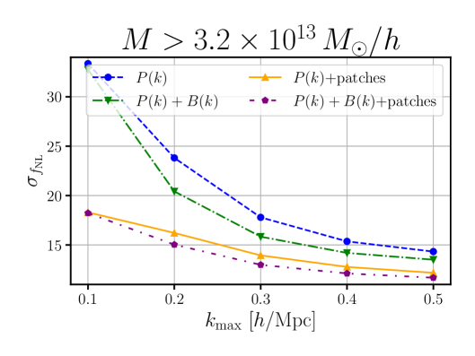
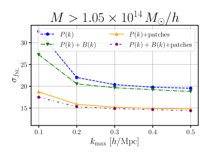
Figure 1: Expected uncertainty for the different summary statistics at $z=1$ for two halo-mass cuts as a function of the power spectrum and bispectrum $k_{\text{max}}$. In both cases, the PatchNet information (patches) improves the constraining power of the power spectrum and the power spectrum combined with bispectrum analyses.

In this work, we aim to combine large- and small-scale information to improve the constraining power over local $f_{\rm NL}$ measurements. A first solution is to use effective field theory to increase the minimum scale we can probe with standard summary statistics. The alternative approach we explored is to use field-level data compression based on machine learning to extract small-scale information, while the large-scale information still comes from standard summary statistics.

The summary statistics we utilise are the power spectrum and the bispectrum. Given the halo over-density, $\delta_{\rm h}$, the power spectrum corresponds to the $2$-point correlation function in Fourier space, and we define it as follows

$$\langle\delta_{\rm h}(\mathbf{k})\,\delta_{\rm h}^{*}(\mathbf{k^{\prime}})\rangle=(2\,\pi)^{3}\,\delta^{\rm D}(\mathbf{k}-\mathbf{k^{\prime}})\,P(k)\,,$$ (4)

where $\delta^{\rm D}$ is the $3$-dimensional Dirac’s delta function. Similarly, we define the halo bispectrum, which is the $3$-point correlation function in Fourier space, as

$$\langle\delta_{\rm h}(\mathbf{k}_{1})\,\delta_{\rm h}(\mathbf{k}_{2})\,\delta_{\rm h}(\mathbf{k}_{3})\rangle=(2\,\pi)^{3}\,\delta^{\rm D}(\mathbf{k}_{1}+\mathbf{k}_{2}+\mathbf{k}_{3})\,B(\mathbf{k}_{1},\mathbf{k}_{2},\mathbf{k}_{3})\,.$$ (5)

To measure the power spectra and bispectra of the simulated boxes, we used the public codes Pylians3 (Villaescusa-Navarro, 2018) and pySpectrum (Scoccimarro, 2015; Hahn et al., 2020), respectively. We measure the power spectra on a $512^{3}$ grid from the fundamental wave number of the box, $k_{\rm f}\sim 0.006\,h\,\text{Mpc}^{-1}$, to $k_{\text{max}}\sim 0.8\,h\,\text{Mpc}^{-1}$ with a $k_{\rm f}$ linear binning; on the other hand, we use a $256^{3}$ grid for the bispectrum, which we measure with a $3\,k_{\rm f}$ linear binning from $k_{\rm min}=3\,k_{\rm f}$ to $k_{\text{max}}\sim 0.5\,h\,\text{Mpc}^{-1}$.

3.3 Field level compression with PatchNet

We employ field-level data compression, using a CNN to extract small-scale information following the approach of Bairagi & Wandelt (2025). The network does not analyse the whole simulated box; it only analyses a sub-cube, which we dub ‘patch’ and call the network PatchNet. The PatchNet approach has two main advantages: first, it reduces the memory requirement for the CNN while maintaining the pixel (or better voxel) resolution, as it processes a smaller volume. Second, the number of training data greatly increases as we can cut out a set of $N_{\text{sb}}$ patches from one simulated box to train the network, effectively increasing the amount of training data by a factor of $N_{\text{sb}}$. As we will explain below, we train PatchNet to compress each patch into one informative statistic, namely the value of $f_{\rm NL}$, and then aggregate these statistics by averaging across the $N_{\text{sb}}$ patches of a given simulated box. We then concatenated this aggregated information with the power spectrum or the combination of the power spectrum and bispectrum.

PatchNet has the following architecture: first, there are three blocks composed of a convolutional layer and a three-dimensional average pooling layer, then their output is flattened and processed by three dense layers before the final output. The convolutional layers, as well as the average pooling, have a $3\times 3\times 3$ kernel with a stride of $1$ and $0$ padding. The first convolutional layer has $8$ filter in output, and the filters are increased by a factor of $4$ in the following layers. After the flattening, the latent features are compressed into $512$ neurons and subsequently halved in number by the other dense layers. Both the convolutional and dense layers have a LeakyReLU (Maas, 2013) with a negative slope of $0.5$ as activation function. We use a modified version of the mean squared error as loss function, which reads as follows

$$\text{Loss}(\mathbf{y},\mathbf{\hat{y}})=\sum_{i}^{n_{\rm b}}\frac{1}{n_{\rm b}}\left(\sum_{j}^{n_{\text{sb}}}\frac{1}{n_{\text{sb}}}y_{j,i}-\sum_{j}^{n_{\text{sb}}}\frac{1}{n_{\text{sb}}}\hat{y}_{j,i}\right)^{2}\,,$$ (6)

where $\mathbf{y}$ are the outputs of PatchNet, $\mathbf{\hat{y}}$ are the labels ($f_{\rm NL}$), $n_{\rm b}$ is the batch size, i.e., the number of simulations we load, and $n_{\text{sb}}$ is the number of patches we use for each simulation. We use $n_{\rm b}=32$ and $n_{\text{sb}}=64$; therefore, a batch actually contains $n_{\rm b}\times n_{\text{sb}}$ different inputs.

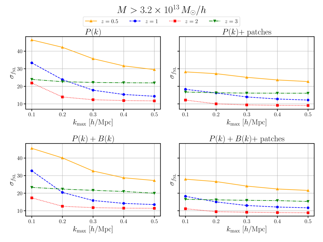
Figure 2: Expected uncertainty for the different summary statistics as a function of the power spectrum and bispectrum $k_{\text{max}}$ at different redshift snapshots. At all redshifts, we applied the same halo-mass cut, $M_{\text{h}}>3.2\times M_{\odot}\,h^{-1}$. The patch information adds constraining power at every redshift.

Before inputting the halo catalogues to the network, we preprocess them. First, we divide the $1000$ simulations with varying $f_{\rm NL}$ into the training, validation, and test sets, which we select with a standard split of $75\%$, $15\%$, and $10\%$ of the data, respectively. Then, we build the patches from the simulated halo catalogue density contrast, which we compute by painting the halos on a $128^{3}$ grid with the cloud in cell (CIC) algorithm. Note that during the painting process, we do not use any halo mass information. We divide the $3$-dimensional number density contrast into $16^{3}$ non-overlapping cubes. This results in $512$ patches for each simulation that have a physical dimension of $125^{3}\,\text{Mpc}^{3}\,h^{-3}$ and a resolution of $8\,\text{Mpc}\,h^{-1}$, which in Fourier space correspond to $k_{\text{min}}\sim 0.05\,h\,\text{Mpc}^{-1}$ and $k_{\text{max}}\sim 0.4\,h\,\text{Mpc}^{-1}$. Finally, before feeding the density contrast patches to the network, we centre and scale them with the mean and standard deviations computed from the density contrast of the fiducial cosmology realisations. We note that we computed these two quantities for each redshift and mass cut configuration (see Sect. 2).

4 Results

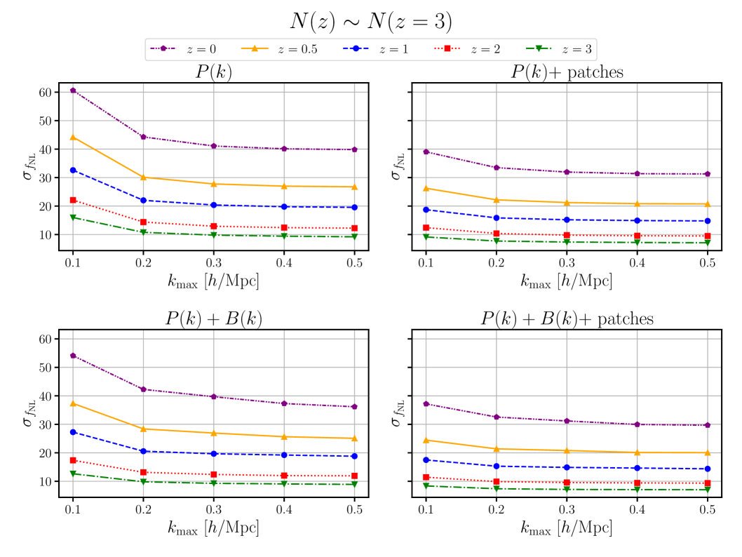
Figure 3: Expected uncertainty for the different summary statistics at fixed number density over redshifts as a function of the power spectrum and bispectrum $k_{\text{max}}$. At each redshift, we selected a halo-mass cut that has in the fiducial cosmology the same number density of $z=3$ (see Table 1). As in Fig. 2, the patch information improves the constraining power of the standard summary statistics.

In this section, we present and discuss the results of the Fisher information analysis. In particular, we compare the information content of the power spectrum and bispectrum with their combination with the patch information.

Figure 1 shows the results of the Fisher information analysis at redshift $z=1$ for two mass cuts as a function of the $k_{\text{max}}$ of the power spectrum and bispectrum. Adding patch information always produces tighter bounds than the standard summary statistics alone. Moreover, we also observe an improvement in the combination of the power spectrum and the patches (solid orange line with triangular markers) with respect to the combined power spectrum and bispectrum (dash-dotted green line with reverse triangular markers), showing that PatchNet extracts information not captured by the 2-point and 3-point functions. This is also backed up by the fact that even though the improvement due to the patch information decreases when $k_{\rm max}$ increases, as the minimum scale probed by the standard summary statistics gets closer to the minimum scale of the patches ($k_{\rm max}^{\rm patch}\sim 0.4\,h\,\text{Mpc}^{-1}$), we still observe an improvement when $k_{\rm max}^{\rm patch}<k_{\rm max}^{P,B}$ point again in the direction that the patches use information beyond the $3$-point function. Nevertheless, the bispectrum still brings a small amount of information that the network cannot extract, as the combination of the three statistics (sparse dash-dotted purple line with pentagonal markers) is always slightly lower than the combination of the power spectrum and patches alone. This behaviour is not unexpected as the bispectrum has access to the very large-scale squeezed triangle configuration, which contains non-Gaussian information that the patches cannot access due to their limited size.

Comparing the left and right panels we see that the overall information content of the smaller mass cut ($M_{\text{min}}=3.2\times 10^{13}\,M_{\odot}\,h^{-1}$, left panel) is higher than the larger mass cut ($M_{\text{min}}=1.05\times 10^{14}\,M_{\odot}\,h^{-1}$, right panel). This is because when the mass cut is smaller, the halo field has lower shot noise and contains more information. However, the improvement related to the patch information is greater in the case of the larger mass cut for $k_{\text{max}}\geq 0.2\,h\,\text{Mpc}^{-1}$. This means that, in terms of real objects, this method is more effective for highly biased objects, e.g., quasars, which we usually utilise to produce surveys with the large volumes that are required for $f_{\rm NL}$ measurements.

We present the constraining power of the different statistics as a function of redshift in Figs. 2 and 3. In Fig. 2 we kept the $M_{\text{min}}$ constant, while in Fig. 3 we varied it as a function of redshift to keep the number density of the catalogues equal to the halo number density at $z=3$. The feature that is common to both plots is that the addition of the patch information always makes the expected error at $k_{\text{max}}=0.1\,h\,\text{Mpc}^{-1}$ comparable to, if not better than, the constraint of the standard summary statistics alone at $k_{\text{max}}=0.5\,h\,\text{Mpc}^{-1}$. This is an interesting result, considering that modelling the power spectrum and bispectrum becomes more involved as we enter the non-linear regime, $k_{\text{max}}>0.1\,h\,\text{Mpc}^{-1}$, requiring a large number of simulations, or EFT to model the observed data. The use of patch information can greatly reduce the effort in the modelling of the standard summary statistics, while requiring a smaller simulation budget than neural estimators acting on the full field.

Finally, the authors of Jung et al. (2023b) have shown that there is a high information content related to $f_{\rm NL}$ in the halo mass function. As some halo mass information is retained in the density contrast, PatchNet may be just learning the relation between the halo mass function and $f_{\rm NL}$, making the field-level analysis superfluous. To check if this is the case, we trained PatchNet keeping the number of objects in the catalogue fixed. The difference between this analysis and the one with constant density is that in the latter, the mass cut was chosen at the fiducial cosmology (with $f_{\rm NL}=0$) and used for all the other simulated cosmologies. Therefore, there was a variation in the number density as a function of $f_{\rm NL}$. On the other hand, for this test, we keep the number of objects fixed even when we vary the value of $f_{\rm NL}$. Doing so, we remove the halo mass function information. Even in this configuration, PatchNet learns a relationship between the density contrast field and $f_{\rm NL}$. In this case, the Pearson correlation coefficient is $r_{\text{w/o HMF}}\sim 0.78$, which we compare with $r_{\text{w HMF}}\sim 0.99$ for the standard configuration. This shows that the network extracts information beyond the halo mass function, as $r_{\text{w HMF}}>r_{\text{w/o HMF}}$. Nevertheless, the halo mass function remains highly informative, with $r\gg 0.50$.

5 Conclusions

In this work, we propose an alternative approach to EFT up to large $k_{\rm max}$ or more standard ML-based field-level algorithms to analyse galaxy redshift surveys. The algorithm combines the large-scale information encoded in the $n$-point summary statistics, such as the power spectrum or bispectrum, with the small-scale information obtained by averaging over the compressed field-level information of small patches of the simulated box, the PatchNet approach (Bairagi & Wandelt, 2025). The main advantage of this approach is that the analysis of small patches is computationally lighter than analysing the whole box; additionally, by cutting the simulated boxes into patches, we greatly increase the number of training examples for the PatchNet (Bairagi et al., 2025). We estimated the Fisher information of this combined summary statistics to extract local PNG information.

We tested the algorithm on the FoF halo catalogues of the Quijote-PNG simulations. We compared its performance with the more standard analyses based on the power spectrum or the combination of the power spectrum and bispectrum. We performed this comparison for different values of $k_{\rm max}$ for the $n$-point statistics and studied it as a function of redshift and for different halo mass cuts.

Our preliminary study shows that the patch-based data compression always provides additional information relative to the standard summary statistics. We observe the largest improvements when the power spectrum and the bispectrum are truncated at $k_{\rm max}=0.1\,h\,\text{Mpc}^{-1}$, where the small-scale structure in the patches provides the most complementary information. At this scale, depending on the redshift, mass cut, and the statistics combination, the improvement varies between $30\%$ and $45\%$. Moreover, when we compare the power spectrum plus bispectrum bounds with the patch-combined bounds (both power spectrum with patches and power spectrum plus bispectrum with patches), again the patches always bring an improvement, proving that they contain information beyond the $3$-point function. Nevertheless, we also observed that combining the bispectrum with the PatchNet compression also provides an improvement, which shows that the large-scale bispectrum encodes information that the patches miss due to their limited size.

A first extension to this work would be to test our method’s performance for other forms of PNG and the effect of marginalising over cosmological parameters. Second, to fully understand the potential of the patch-based approach, it would be of interest to compare its information content with other alternative summary statistics, e.g., wavelet scattering transform (e.g., Peron et al., 2024) or a marked power spectrum (e.g., Marinucci et al., 2025). Additionally, to ready this approach for application to data, we will need to introduce a galaxy model in the simulations and understand how to treat the lightcone, the survey mask, and systematic effects. We plan to study these issues in future work.