Enhanced Angle-Range Cluster Parameter Estimation in Full-Duplex ISAC Systems

Abstract

This work studies an integrated sensing and communication (ISAC) framework for targets that are spread both in the angle and range domains. We model each target using a cluster of rays parameterized by a specific density function, and propose a truncated Multiple Signal Classification (MUSIC) spread (TMS) algorithm to accurately estimate the parameters of the density function. Unlike the conventional MUSIC spread (CMS), TMS restricts the signal subspace rank based on the eigen decomposition of the received-signal autocorrelation. We also propose a discrete Fourier transform (DFT) based algorithm for estimating the distance and range spread of each target. Leveraging these estimates, we then develop a dynamic transmit beamforming algorithm that successfully illuminates multiple targets while also serving multiple downlink (DL) users. Simulation results demonstrate the superiority of our proposed algorithms over baseline schemes in both low and high signal-to-noise ratio (SNR) regimes as well as under a wide angular spread regime.

I Introduction

Integrated sensing and communication (ISAC) systems have been one of the most important areas of research for next-generation sixth generation (6G) wireless systems [1, 2]. In ISAC systems, different taxonomies have been investigated based on the system model and waveform design in the literature [3]. For instance, from a system modeling perspective, device-free and device-based sensing scenarios have been investigated [4], while in the waveform design aspect, communication-centric, radar-centric, and joint-design strategies have been explored and advanced in recent years [5, 6].

Despite the recent advancements in ISAC literature, most of the works do not focus on the modeling aspect of radar targets [7, 8]. For instance, in most communication-centric design studies, both sensing targets and communication users have been modeled as point objects in the far field of transmitter (TX) antennas [9, 10, 11]. This modeling aspect is acceptable for communication purposes as the receiver (RX) antennas occupy a significantly small area; however, for sensing in vehicle-to-infrastructure (V2I) and vehicle-to-everything (V2X) settings, this assumption becomes invalid. Realizing this, many research groups have focused their attention on the extended target (ET) model, where each target is modeled as either a large number of scatterers [12, 13], or to use a parametric model to define a contour of the target, such as truncated Fourier series (TFS) [14, 15]. Although these models can model complex targets, they do so at a much higher computational cost. For instance, in both these strategies, either all of the scatterers or a large number of parameters are needed to fully characterize the target. In addition, these models consider deterministic settings and hence forgo the stochastic nature of the radar channel.

In an effort to address these limitations, we use a parametric cluster ray (CR) target model, in which each target is modeled as a cluster of rays with corresponding densities in both the angular and range domains. Based on this, the main contributions of our work are:

• Realizing the computational complexities of target modeling in recent works [14, 15], we use a computationally efficient CR model for a target – proposed in $3^{\mathrm{r}d}$ Generation Partnership Project (3GPP) [16]. To the best of our knowledge, this is the first attempt to study a spatially spread or clustered target in the context of ISAC systems.

• We propose truncated MUSIC spread (TMS) and TMS-approx methods for estimating angular parameters (direction and angular spread). For range parameters (distance and range spread), we propose a discrete Fourier transform (DFT) based approach in which thresholding (in the time domain) is used to extract the parameters.

• We propose a fast dynamic beam pattern synthesis algorithm that maximizes expected radar signal to noise ratio (SNR) while satisfying multi-user achievable rate constraints. Unlike recent works [14], we synthesize the required beam pattern without explicitly mentioning the beam pattern matching constraints.

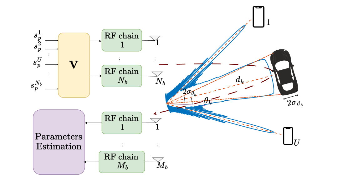
Figure 1: System Model where FD-ISAC BS serves $U$ DL communication users along with sensing of $K$ CR targets.

II System Model

We consider a multiple input multiple output (MIMO) FD ISAC system operating at millimeter-Wave (mmWave) frequencies using orthogonal frequency division multiplexing (OFDM) waveforms. We assume that over a single symbol, BS transmits information over $P$ subcarriers for $U$ users as presented in Fig. 1. BS node also estimates the angular (direction and angular spread) as well as temporal (distance and range spread) parameters of CR target. We assume that BS is equipped with $N_{b}$ transmit, and $M_{b}$ receive antennas and transmits $U$ independent information signals (for $U$ users) as well as $N_{b}-U$ artificial sensing signals. The information symbol at $p^{\mathrm{th}}$ subcarrier can then be given as $\mathbf{s}_{p}=\begin{bmatrix}\mathbf{s}_{U}^{\mathrm{T}}&\mathbf{s}_{R}^{\mathrm{T}}\end{bmatrix}^{\mathrm{T}}\in\mathbb{C}^{N_{b}\times 1}$ where $\mathbf{s}_{U}\in\mathbb{C}^{U\times 1}$ is intended for $U$ users while $\mathbf{s}_{R}\in\mathbb{C}^{N_{b}-U\times 1}$ is an artificially created radar signal which is uncorrelated to the communication signals i.e., $\mathbb{E}\left(\mathbf{s}_{R}\mathbf{s}_{U}^{\mathrm{H}}\right)=\mathbf{0}$ and $\mathbb{E}\left(\mathbf{s}_{p}\mathbf{s}_{p}^{\mathrm{H}}\right)=\mathbf{I}$. This information signal then undergoes digital beamforming that maps different streams to different transmit antennas. The overall transmit signal at $p^{\mathrm{th}}$ subcarrier is defined as

$$\mathbf{x}_{p}=\mathbf{V}_{U}\mathbf{s}_{U}+\mathbf{V}_{R}\mathbf{s}_{R}=\mathbf{V}\mathbf{s}_{p}$$ (1)

where $\mathbf{V}_{U}\in\mathbb{C}^{N_{b}\times U}$ and $\mathbf{V}_{R}\in\mathbb{C}^{N_{b}\times N_{b}-U}$ are beamforming matrices for $U$ users and sensing the CR targets. We define the set of users as: $\mathcal{L}\triangleq\{1,2,\cdots,U\}$. For target modeling, we denote $N_{p}$ as the number of rays per cluster, $\alpha_{k,r}$ as the reflection coefficient of the $r^{\mathrm{th}}$ ray of the $k^{\mathrm{th}}$ cluster. To make our analysis tractable, we assume $N_{b}=M_{b}$. Moreover, we represent the array response vector of direction $\theta$ as $\mathbf{a}(\sin(\theta))=[e^{-j\pi\frac{N_{b}-1}{2}\sin(\theta)},\cdots,e^{j\pi\frac{N_{b}-1}{2}\sin(\theta)}]^{\mathrm{T}}$. The radar channel at $p^{\mathrm{th}}$ subcarrier can then be given as

$$\mathbf{H}_{\mathrm{rad}}^{p}=\sqrt{\kappa}\sum_{k=1}^{K}\sum_{r=1}^{N_{p}}\alpha_{k,r}\omega_{k,r}^{p}\mathbf{A}(\sin(\theta_{k,r})),$$ (2)

where $\mathbf{A}(\sin(\theta_{k,r}))\triangleq\mathbf{a}(\sin(\theta_{k,r}))\mathbf{a}^{\mathrm{H}}(\sin(\theta_{k,r}))$, $\kappa=\frac{N_{b}M_{b}}{N_{p}}$, $\omega_{k,r}^{p}=e^{-j2\pi p\Delta f\tau_{k,r}}$ denote the phase shift across subcarriers due to the target distance, $\Delta f=\frac{1}{T_{\mathrm{OFDM}}+T_{\mathrm{CP}}}$ is the subcarrier spacing ($T_{\mathrm{OFDM}}$ and $T_{\mathrm{CP}}$ represents the symbol time and cyclic prefix respectively), $\tau_{k,r}=\frac{2d_{k,r}}{c}$ represent the time delay due to the ray distance $d_{k,r}$ from the BS and $c$ denote the speed of light. We assume that the distance follows a certain symmetric probability distribution $f_{D_{k}}(d)$ with a mean distance ($d_{k}$) and range spread ($\sigma_{d_{k}}$). Moreover, $\theta_{k,r}$ represents the direction of the $r^{\mathrm{th}}$ ray of the $k^{\mathrm{th}}$ cluster, and it also follows a symmetric spatial distribution $f_{\Theta_{k}}(\theta)$ with a certain mean angle ($\theta_{k}$) and angular spread ($\sigma_{\theta_{k}}$). We represent all the estimation parameters in a vector as $\boldsymbol{\eta}$. We assume a self-interference (SI) cancellation receiver at the BS, presented in [11, 10], and hence our focus will be on the baseband received signal after analog and digital SI cancellation. The post-cancellation signal is given as

$$\mathbf{y}_{p}=\mathbf{H}_{\mathrm{rad}}^{p}\mathbf{x}_{p}+\mathbf{z}_{p}$$ (3)

where $\mathbf{z}_{p}\in\mathbb{C}^{M_{b}}$ is the residual SI and noise vector whose each entry is independent and identically distributed (IID) complex Gaussian distributed with zero mean and variance $\sigma_{b}^{2}$, i.e., $\mathbf{z}_{p}\sim\mathcal{CN}\left(\mathbf{0},\sigma_{b}^{2}\mathbf{I}_{M_{b}}\right)$. Similarly the DL channel of user $u\in\mathcal{L}$ is given as

$$\mathbf{h}_{u}^{\mathrm{H}}=\sqrt{N_{b}}\beta_{u}\mathbf{a}_{\mathrm{N_{b}}}^{\mathrm{H}}(\phi_{u}),$$ (4)

where $\beta_{u}$ and $\phi_{u}$ represent the channel coefficient and the LOS direction from the BS. The received signal at the $p^{\mathrm{th}}$ subcarrier at user $u$ is given as

$$r_{u}^{p}=\mathbf{h}_{u}^{\mathrm{H}}(\mathbf{v}_{u}s_{p}^{u}+\sum_{u^{\prime}\neq u}^{N_{b}}\mathbf{v}_{u^{\prime}}s_{p}^{u^{\prime}})+z_{u}^{p},$$ (5)

where $\mathbf{v}_{u}$ is the $u^{\mathrm{th}}$ column of $\mathbf{V}$, $s_{p}^{u}$ is the $u^{\mathrm{th}}$ entry of vector $\mathbf{s}_{p}$, and $z_{u}$ represents the noise at the user $u$ following a complex Gaussian distribution with zero mean and variance $\sigma_{u}^{2}$. The main objective of the ISAC system is to 1) serve all the $U$ users in the environment and 2) estimate $\boldsymbol{\eta}$, and 3) design a beam pattern to illuminate all of the LOS faces of all the targets $K$. Now we present the parameter estimation methods, followed by a beamforming optimization scheme based on the estimated parameters.

III Parameter Estimation

At the RX of the BS node $b$, we first utilize all the streams to estimate the angular characteristics, followed by the range and range spread. Hence, we split our estimation vector $\boldsymbol{\eta}$ in two sub vectors: $\boldsymbol{\eta}=\begin{bmatrix}\boldsymbol{\eta}_{1}^{\mathrm{T}}&\boldsymbol{\eta}_{2}^{\mathrm{T}}\end{bmatrix}^{\mathrm{T}}$, where $\boldsymbol{\eta}_{1}=\begin{bmatrix}\boldsymbol{\theta}^{\mathrm{T}}&\boldsymbol{\sigma}_{\theta}^{\mathrm{T}}\end{bmatrix}^{\mathrm{T}}$ and $\boldsymbol{\eta}_{2}=\begin{bmatrix}\mathbf{d}^{\mathrm{T}}&\boldsymbol{\sigma}_{d}^{\mathrm{T}}\end{bmatrix}^{\mathrm{T}}$ where $\boldsymbol{\theta}$ consists of direction, $\boldsymbol{\sigma}_{\theta}$ consists angular spreads, $\boldsymbol{\mathbf{d}}$ consists of distances, and $\boldsymbol{\sigma}_{d}$ consists of all range spreads. In order to estimate $\boldsymbol{\eta}_{1}$, we use the auto-covariance matrix of the received signal $\mathbf{y}_{p}$, while for estimating $\boldsymbol{\eta}_{2}$, we use the conditional expected value of the received signal. We first propose the algorithm for estimating $\boldsymbol{\eta}_{1}$, followed by an estimator of range parameters in $\boldsymbol{\eta}_{2}$.

III-A Proposed Subspace-based TMS for angular parameters

For estimating the angular parameters, we use the autocorrelation matrix of the received signal at the BS, which will be $\mathbf{R}_{\mathbf{Y}}\triangleq\mathbb{E}\left[\mathbf{y}_{p}\mathbf{y}_{p}^{\mathrm{H}}\ \right]=\mathbf{R}_{\mathbf{Y}}^{\mathrm{sen}}+\sigma_{b}^{2}\mathbf{I}=\mathbb{E}\left[\mathbf{x}_{p}^{\mathrm{H}}\left(\mathbf{H}_{\mathrm{rad}}^{p}\right)^{\mathrm{H}}\mathbf{H}_{\mathrm{rad}}^{p}\mathbf{x}_{p}\right]+\sigma_{b}^{2}\mathbf{I}$, where the expectation is with respect to $d_{k,r}$, $\theta_{k,r}$, $\mathbf{x}_{p}$, and $\mathbf{z}_{p}$. We define $\mathbf{R}_{\mathbf{X}}=\mathbb{E}(\mathbf{x}_{p}\mathbf{x}_{p}^{\mathrm{H}})$ and simplify $\mathbf{R}_{\mathbf{Y}}^{\mathrm{sen}}$ as follows

$$\mathbf{R}_{\mathbf{Y}}^{\mathrm{sen}} =\kappa\sum_{k,r}\lvert\alpha_{k,r}\rvert^{2}\mathbf{J}(\theta_{k},\sigma_{\theta_{k}}),$$ (6)

where $\mathbf{J}(\theta_{k},\sigma_{\theta_{k}})\triangleq\mathbb{E}\left[\mathbf{A}(\sin(\theta_{k,r}))\mathbf{R}_{\mathbf{X}}\mathbf{A}^{\mathrm{H}}(\sin(\theta_{k,r}))\right]$. In (6), complex exponential terms like $e^{jc\sin(\theta)}$, where $c$ is a constant and $\theta$ in random variable (RV), can be expanded using Jacobi-Anger expansion as $e^{jc\sin(\theta)}=J_{0}(c)+2\sum_{n=1}^{\infty}J_{2n}(b)\cos(2n\theta)+2j\sum_{n=1}^{\infty}J_{2n-1}(c)\sin((2n-1)\theta)$, where $J_{n}(z)$ is the $n^{\mathrm{th}}$ Bessel function of first kind. In order to avoid this infinite summation, we utilize the following approximation for the random angle $\theta_{k,r}$, assuming that the perturbation around the mean angle is small, then $\sin(\theta_{k,r})=\sin(\theta_{k}+\tilde{\theta}_{k,r})\approx\sin(\theta_{k})+\tilde{\theta}_{k,r}\cos(\theta_{k})$. Using this approximation, the matrix $\mathbf{A}(\sin(\theta_{k,r}))$ can be approximated as

$$\mathbf{A}(\sin(\theta_{k,r})) \approx\mathbf{A}(\sin(\theta_{k}))\odot\mathbf{A}(\tilde{\theta}_{k,r}\cos(\theta_{k}))$$

$$=\mathbf{D}(\sin(\theta_{k})) \mathbf{A}(\tilde{\theta}_{k,r}\cos(\theta_{k}))\mathbf{D}^{\mathrm{H}}(\sin(\theta_{k})).$$ (7)

where $\mathbf{D}(\sin(\theta_{k}))=\mathrm{diag}(\mathbf{a}(\sin(\theta_{k})))$. Using this and exploiting the vectorization operator, we can find the closed form expression of $\mathbf{J}(\theta_{k},\sigma_{\theta_{k}})$ as

$$\mathbf{J}(\theta_{k},\sigma_{\theta_{k}}) =\mathrm{vec}^{-1}\Bigl(\widetilde{\mathbf{D}}(\sin(\theta_{k}))\widetilde{\boldsymbol{\Phi}}_{k}\widetilde{\mathbf{D}}^{\mathrm{H}}(\sin(\theta_{k}))$$

$$\times\mathrm{vec}\left(\mathbf{R}_{\mathbf{X}}\right)\Bigr),$$ (8)

proof: Proof is omitted for brevity, but it can easily be derived using the inverse vectorization operator and identity $\mathrm{vec}(\mathbf{A}\mathbf{B}\mathbf{C})=(\mathbf{C}^{\mathrm{T}}\otimes\mathbf{A})\mathrm{vec}(\mathbf{B})$. The definition of $\widetilde{\mathbf{D}}(\sin(\theta_{k}))$ and $\widetilde{\boldsymbol{\Phi}}_{k}$ are given as

$$\widetilde{\mathbf{D}}(\sin(\theta_{k}))=\mathrm{diag}\left(\mathbf{a}^{*}(\sin(\theta_{k}))\otimes\mathbf{a}(\sin(\theta_{k}))\right),$$ (9)

$$\widetilde{\boldsymbol{\Phi}}_{k}=\mathbb{E}\left(\mathbf{A}^{*}(\tilde{\theta}_{k,r}\cos(\theta_{k}))\otimes\mathbf{A}(\tilde{\theta}_{k,r}\cos(\theta_{k}))\right).$$ (10)

The terms involved in (10), can be evaluated as $\mathbb{E}\left[e^{j\varrho_{k}(l+m-n)\tilde{\theta}_{k,r}}\right]=\psi_{\tilde{\theta}_{k,r}}(\varrho_{k}(m-n+l))$, where $\varrho_{k}=\pi\cos(\theta_{k})$, and $\psi_{\tilde{\theta}_{k,r}}(.)$ is the characteristic function of RV $\tilde{\theta}_{k,r}$. In our paper, we assume $\tilde{\theta}_{k,r}\sim\mathcal{U}\left[-\delta_{\theta_{k}},\delta_{\theta_{k}}\right]$ (where $\delta_{\theta_{k}}=\sqrt{3}\sigma_{\theta_{k}}$), then

$$\psi_{\tilde{\theta}_{k,r}}(t\varrho_{k}) =\mathrm{sinc}(t\varrho_{k}\delta_{\theta_{k}}),$$ (11)

where $t=m-n+l$, and $\mathrm{sinc}(x)=\sin(x)/x$. Based on the above analysis, we note that the matrix $\mathbf{J}(\theta_{k},\sigma_{\theta_{k}})$ is independent of individual ray characteristics, and exploiting this fact, the eigen decomposition of (6) is given as $\mathbf{R}_{\mathbf{Y}}^{\mathrm{sen}}=\mathbf{E}_{\mathrm{s}}\boldsymbol{\Lambda}_{\mathrm{s}}\mathbf{E}_{\mathrm{s}}^{\mathrm{H}}+\mathbf{E}_{\mathrm{n}}\boldsymbol{\Lambda}_{\mathrm{n}}\mathbf{E}_{\mathrm{n}}^{\mathrm{H}},$ where $\mathrm{s}$ represents signal subspace while $\mathrm{n}$ represents noise sub space. Although $\mathbf{R}_{\mathbf{Y}}^{\mathrm{sen}}$ might be of full rank, most of the energy is encapsulated in the first $q$ eigenvalues [18]. In actuality, we will have the estimates of $\mathbf{R}_{\mathbf{Y}}^{\mathrm{sen}}$, denoted with $\hat{\mathbf{R}}_{\mathbf{Y}}^{\mathrm{sen}}$, and we represent its corresponding eigen decomposition with a hat as well. Then we define the spread MUSIC spectrum as

$$\mathrm{P}_{\mathrm{TMS}}(\theta,\sigma_{\theta})=\frac{1}{\lvert\lvert\widehat{\mathbf{E}}_{\mathrm{n}}^{\mathrm{H}}{\mathbf{E}}_{s}(\theta,\sigma_{\theta})\rvert\rvert_{\mathrm{F}}^{2}},\,\,\forall\theta\in\mathcal{T}_{\theta},\sigma_{\theta}\in\mathcal{T}_{\sigma_{\theta}}$$ (12)

where ${\mathbf{E}}_{s}(\theta,\sigma_{\theta})$ is the first $q$ eigen vectors of $\mathbf{J}(\theta,\sigma_{\theta})$ stacked in columns. $\mathcal{T}_{\theta}$ and $\mathcal{T}_{\sigma_{\theta}}$ are search regions for $\theta$ and $\sigma_{\theta}$ which are discretized in a grid.
Remark: Note that, unlike [18, 17] where $\mathbf{E}_{s}(\theta,\sigma_{\theta})=\mathbf{J}(\theta,\sigma_{\theta})$, we do the eigen decomposition of $\mathbf{J}(\theta,\sigma_{\theta})$. The reason is that, in DOA estimation of distributed signals (DISPARE) or conventional MUSIC spread (CMS), following estimates are utilized [17]

$$\{\theta_{k},\sigma_{\theta_{k}}\}=\arg\min_{\theta_{k},\sigma_{\theta_{k}}}\left\lvert\left\lvert\mathbf{E}_{n}^{\mathrm{H}}\mathbf{J}(\theta_{k},\sigma_{\theta_{k}})\right\rvert\right\rvert_{\mathrm{F}}^{2}.$$ (13)

If we expand this function, we get

$$f_{k} =\left\lvert\left\lvert\mathbf{E}_{n}^{\mathrm{H}}\mathbf{J}(\theta_{k},\sigma_{\theta_{k}})\right\rvert\right\rvert_{\mathrm{F}}^{2}$$

$$=\mathrm{Tr}\Bigl(\mathbf{E}_{n}^{\mathrm{H}}\bigl(\mathbf{E}_{s}(\theta_{k},\sigma_{\theta_{k}})\boldsymbol{\Lambda}^{2}_{s}(\theta_{k},\sigma_{\theta_{k}})\mathbf{E}_{s}^{\mathrm{H}}(\theta_{k},\sigma_{\theta_{k}})$$

$$+\mathbf{E}_{n}(\theta_{k},\sigma_{\theta_{k}})\boldsymbol{\Lambda}^{2}_{n}(\theta_{k},\sigma_{\theta_{k}})\mathbf{E}_{n}^{\mathrm{H}}(\theta_{k},\sigma_{\theta_{k}})\bigr)\mathbf{E}_{n}\Bigr)$$ (14)

At true parameters, the first in (14) term will vanish and we will be left with $\overset{*}{f}_{k}=\mathrm{Tr}\left(\boldsymbol{\Lambda}^{2}_{n}(\theta_{k},\sigma_{\theta_{k}})\right)$. It is possible that some other parameter vector decreases the second term more than the increase of the first term, and hence the peak at true parameters will not be the global minimum of the cost function [19]. In order to avoid this, we do the eigen decomposition of $\mathbf{J}(\theta_{k},\sigma_{\theta_{k}})$ as well.

In order to find the $q$, we utilize the following test

$$\overset{*}{q}=\min\{q\,\,|\frac{\sum_{i=1}^{q}\lambda_{i}}{\mathbf{1}^{\mathrm{T}}\boldsymbol{\Lambda}\mathbf{1}}\geq\chi\},$$ (15)

where $\chi\in[0,1]$ is a design variable, that tells the fraction of total energy should we include in our signal space and $\lambda_{i}$ is the $i^{\mathrm{th}}$ diagonal entry of the matrix $\boldsymbol{\Lambda}$, which is the diagonal matrix of eigen values of the matrix $\mathbf{R}_{\mathbf{Y}}^{\mathrm{sen}}-\sigma_{b}^{2}\mathbf{I}$. Using (12), the estimate of vector $\boldsymbol{\eta}_{1}$ is given as

$$\begin{aligned} \hat{\boldsymbol{\eta}}_{1}=\operatornamewithlimits{argmax}_{\boldsymbol{\eta}_{1}}\quad\mathrm{P}_{\mathrm{TMS}}(\boldsymbol{\eta}_{1}).\end{aligned}$$ (16)

One can note here that the evaluation of the matrix $\mathbf{J}(\theta_{k},\sigma_{\theta_{k}})$ also depends on the matrix $\mathbf{V}$. Moreover, as an intermediate step, we also need to compute a big matrix of size $M_{b}^{2}\times N_{b}^{2}$ before inverse vectorization, and hence both of these tasks are computationally expensive and repetitive for different $\mathbf{V}$. To address this, we also present a low complexity estimator based on the conditional mean of the received signal in the next section.

III-B Low Complexity TMS for angular parameters

Using the approximation defined on (7), we start with the conditional expectation of the received signal in (3) given the noise and the transmitted signal as follows

$$\mathbb{E}\bigl(\mathbf{y}_{p}|\mathbf{x}_{p},\mathbf{z}_{p}\bigr)\overset{(b)}{\approx}\sqrt{\kappa}\sum_{k,r}\alpha_{k,r}\psi_{d_{k,r}}\left(\frac{4\pi p\Delta f}{c}\right)\mathbf{D}(\sin(\theta_{k}))$$

$$\times\boldsymbol{\Phi}_{k}\mathbf{D}^{\mathrm{H}}(\sin(\theta_{k}))\mathbf{x}_{p}+\mathbf{z}_{p},$$ (17)

where in ($b$), we utilize the independence of $\mathbf{d}_{k,r}$ and $\theta_{k,r}$, and the matrix $\boldsymbol{\Phi}_{k}=\mathbb{E}(\mathbf{A}(\sin(\theta_{k,r})))$, whose $(m,n)$-th element is given as $[\boldsymbol{\Phi}_{k}]_{m,n}=\psi_{\tilde{\theta}_{k,r}}(\pi(m-n)\cos(\theta_{k}))$, and $\psi_{d_{k,r}}(t)$ is the characteristic function of random variable $d_{k,r}$ which we will find in the next section. The autocorrelation matrix of (17) is given as

$$\widetilde{\mathbf{R}}_{\mathbf{Y}}^{\mathrm{sen}} =\mathbb{E}\left(\mathbb{E}\left(\mathbf{y}_{p}|\mathbf{x}_{p},\mathbf{z}_{p}\right)\left(\mathbb{E}\left(\mathbf{y}_{p}|\mathbf{x}_{p},\mathbf{z}_{p}\right)\right)^{\mathrm{H}}\right)$$

$$\approx\kappa\sum_{k,r}\left\lvert\left\lvert\boldsymbol{\alpha}_{k}\right\rvert\right\rvert^{2}\left\lvert\psi_{d_{k,r}}\left(l_{p}\right)\right\rvert^{2}\mathbf{J}_{\mathrm{app}}(\theta_{k},\sigma_{\theta_{k}})$$

$$\times\mathbf{R}_{\mathbf{X}}\mathbf{J}_{\mathrm{app}}^{\mathrm{H}}(\theta_{k},\sigma_{\theta_{k}})+\sigma_{b}^{2}\mathbf{I},$$ (18)

where $\boldsymbol{\alpha_{k}}=\begin{bmatrix}\alpha_{k,1}&\alpha_{k,2}&\cdots&\alpha_{k,{N_{p}}}\end{bmatrix}^{\mathrm{T}},$ $l_{p}=\frac{4\pi p\Delta f}{c}$, and $\mathbf{J}_{\mathrm{app}}(\theta_{k},\sigma_{\theta_{k}})=\mathbf{D}(\sin(\theta_{k}))\boldsymbol{\Phi}_{k}\mathbf{D}^{\mathrm{H}}(\sin(\theta_{k})).$ Now, the matrix $\mathbf{J}_{\mathrm{app}}(\theta_{k},\sigma_{\theta_{k}})$ is independent of $\mathbf{V}$ and can be precomputed and stored in the memory. Moreover, for each $k$, the terms $\left\lvert\left\lvert\boldsymbol{\alpha}_{k}\right\rvert\right\rvert^{2}$ and $\left\lvert\psi_{d_{k,r}}\left(l_{p}\right)\right\rvert^{2}$ are only scaling parameters and will not affect the signal space. Based on $\mathbf{J}_{\mathrm{app}}(\theta,\sigma_{\theta})$, we use the following low complexity TMS estimator

$$\mathrm{P}_{\mathrm{TMS}}^{\mathrm{app}}(\theta,\sigma_{\theta})=\frac{1}{\left\lvert\left\lvert\widehat{\mathbf{E}}_{n}^{\mathrm{H}}{\mathbf{E}}_{s}^{\mathrm{app}}(\theta,\sigma_{\theta})\right\rvert\right\rvert},\,\forall\theta\in\mathcal{T}_{\theta},\sigma_{\theta}\in\mathcal{T}_{\sigma_{\theta}}$$ (19)

where ${\mathbf{E}}_{s}^{\mathrm{app}}(\theta,\sigma_{\theta})$ consists of first $q$ eigen vectors of matrix $\mathbf{J}_{\mathrm{app}}(\theta,\sigma_{\theta})\mathbf{R}_{\mathbf{X}}\mathbf{J}^{\mathrm{H}}_{\mathrm{app}}(\theta,\sigma_{\theta})$ stacked in a column, and $q$ is selected based on criteria defined in (15). Then the estimates of $\boldsymbol{\eta}_{1}$ are given as

$$\hat{\boldsymbol{\eta}}_{1}=\operatornamewithlimits{argmax}_{\boldsymbol{\eta}_{1}}\quad\mathrm{P}_{\mathrm{TMS}}^{\mathrm{app}}(\boldsymbol{\eta}_{1}).$$ (20)

III-C Range Parameters Estimation

We assume a symmetric range distribution around the mean distance ($d_{k}$) for each target, and therefore we can express the distance of the $r^{\mathrm{th}}$ ray of the target $k$ as $d_{k,r}=d_{k}+\tilde{d}_{k,r}$, $\tilde{d}_{k,r}$ is a random symmetric perturbation around $d_{k}$. In particular, in our setting we assume that $\tilde{d}_{k,r}$ follows a uniform distribution, that is, $\tilde{d}_{k,r}\sim\mathcal{U}(-\delta_{d_{k}},\delta_{d_{k}})$, where $\delta_{d_{k}}=\sqrt{3}\sigma_{d_{k}}$. In order to estimate the parameters, we begin with the expression (17) and define $\bar{\mathbf{y}}_{p}^{k}=\mathbf{J}_{\mathrm{app}}(\theta_{k},\sigma_{\theta_{k}})\mathbf{x}_{p}$. Then the expected value of $\omega_{k,r}^{p}$ can be evaluated as $\mathbb{E}(\omega_{k,r}^{p})=\psi_{d_{k,r}}(l_{p})=\mathbb{E}(e^{-j2\pi p\Delta f\frac{2d_{k,r}}{c}})=e^{-jl_{p}}\psi_{\tilde{d}_{k,r}}(l_{p})$, where $\psi_{\tilde{d}_{k,r}}(t)$ is the characteristic function of $\tilde{d}_{k,r}$ and is given as: $\psi_{\tilde{d}_{k,r}}(t)={\mathrm{sinc}}(4\pi p\Delta f\delta_{d_{k}}/c)$. Inserting these values in (17) will yield

$$\mathbb{E}\left(\mathbf{y}_{p}|\mathbf{x}_{p},\mathbf{z}_{p}\right)=\sqrt{\kappa}\sum_{k,r}\alpha_{k,r}\psi_{d_{k,r}}(l_{p})\bar{\mathbf{y}}_{p}^{k}+\mathbf{z}_{p}$$ (21)

Using the estimated $\theta_{k}$’s and $\sigma_{\theta_{k}}$’s, we can estimate $\bar{\mathbf{y}}_{p}^{k}$ and divide the received signal by it i.e.,

$$\tilde{\boldsymbol{\mu}}_{p}^{k} =\sqrt{\kappa}\sum_{r=1}^{N_{p}}\alpha_{k,r}\psi_{d_{k,r}}(l_{p})\bar{\mathbf{y}}_{p}^{k}./\hat{\bar{\mathbf{y}}}_{p}^{k}$$

$$+\sqrt{\kappa}\sum_{k^{\prime}\neq k,r}\alpha_{k^{\prime},r}\psi_{d_{k,r}}(l_{p})\bar{\mathbf{y}}_{p}^{k^{\prime}}./\hat{\bar{\mathbf{y}}}_{p}^{k}+\mathbf{z}_{p}./\hat{\bar{\mathbf{y}}}_{p}^{k},$$ (22)

where $\hat{\bar{\mathbf{y}}}_{p}^{k}=\mathbf{J}_{\mathrm{app}}(\hat{\theta}_{k},\hat{\sigma}_{\theta_{k}})\mathbf{x}_{p}$. If $\hat{\theta}_{k}\approx\theta_{k}$ and $\hat{\sigma}_{\theta_{k}}\approx\sigma_{\theta_{k}}$, then the first term in (22) is the phase shifted version of frequency response of $\mathrm{rect}$ function i.e.,

$$\mathcal{F}\left(\mathrm{rect}\left(\frac{t-\tau}{2\delta}\right)\right)\to 2\delta{\mathrm{sinc}}\left(2\pi f\delta\right)e^{-j2\pi f\tau}$$ (23)

where $\mathcal{F}(.)$ is FFT operator. In OFDM frequency axis is discretized in terms of subcarrier indices and spacing. Hence, if we perform inverse discrete Fourier transform (IDFT) operation over the subcarrier indices, we can effectively get the mean range and range spread, i.e., we perform the following IDFT operation on $\tilde{\boldsymbol{{\mu}}}_{p}^{k}$

$$Q(p^{\prime})=\left\lvert\sum_{p=1}^{P}(\mathbf{1}^{\mathrm{T}}\tilde{\boldsymbol{\mu}}_{p}^{k})e^{j2\pi pp^{\prime}/P}\right\rvert^{2}$$ (24)

As mentioned before, in the time domain, we expect to get a rect function. To estimate the parameters of rect, $Q_{\mathrm{max}}$ denote the max term of the $Q(p^{\prime})\,\forall\,p^{\prime}$, then we do the following test

$$\overset{*}{p^{\prime}}_{\mathrm{min}} =\min\left\{p^{\prime}|\frac{Q(p^{\prime})}{Q_{\mathrm{max}}}\geq\eta\right\},$$ (25)

$$\overset{*}{p^{\prime}}_{\mathrm{max}} =\max\left\{p^{\prime}|\frac{Q(p^{\prime})}{Q_{\mathrm{max}}}\geq\eta\right\},$$ (26)

$$\hat{d}_{k} =c\frac{\overset{*}{p^{\prime}}_{\mathrm{min}}+\overset{*}{p^{\prime}}_{\mathrm{max}}}{4\Delta fP},$$ (27)

$$\hat{\sigma}_{d_{k}} =c\frac{\overset{*}{p^{\prime}}_{\mathrm{max}}-\overset{*}{p^{\prime}}_{\mathrm{min}}}{4\sqrt{3}\Delta fP}.$$ (28)

where $\eta\in[0,1]$ defines the threshold above the noise floor.

IV Optimization Problem and its solution

In this section, we will present a framework for optimizing the transmit beamformer $\mathbf{V}$ in order to maximize radar SNR from each target as well as to satisfy user data rate constraints. The optimization problem we aim to solve is:

$$\max_{\mathbf{V}}\quad \gamma_{\mathrm{rad}}=\frac{\mathbb{E}\left[\left\lvert\left\lvert\mathbf{H}_{\mathrm{rad}}^{p}\mathbf{V}\right\rvert\right\rvert_{\mathrm{F}}^{2}\right]}{\sigma_{b}^{2}}$$ (29a)

s.t. $$\Gamma_{u}=\log_{2}\left(1+\gamma_{u}^{\mathrm{sinr}}\right)\geq\gamma_{u},\quad\forall u\in\mathcal{L},$$ (29b)

$$\quad\left\lvert\left\lvert\mathbf{V}\right\rvert\right\rvert_{\mathrm{F}}^{2}\leq\mathrm{P}_{b},$$ (29c)

where $\gamma_{u}^{\mathrm{sinr}}=\frac{\left\lvert\left\lvert\mathbf{h}_{u}^{\mathrm{H}}\mathbf{v}_{u}\right\rvert\right\rvert_{2}^{2}}{\sum_{u^{\prime}\neq u}^{N_{b}}\left\lvert\left\lvert\mathbf{h}_{u}^{\mathrm{H}}\mathbf{v}_{u^{\prime}}\right\rvert\right\rvert_{2}^{2}+\sigma_{u}^{2}}$. Note that, unlike [15, 14], we don’t have an explicit beam pattern matching constraint for each target; the desired beam pattern requirement is implicitly present in the objective function of (29).

To solve (29), we first reformulate the objective function and evaluate the expectation operator involved in $\gamma_{\mathrm{rad}}$. We denote the numerator of $\gamma_{\mathrm{rad}}$ as $\gamma_{\mathrm{rad}}^{\mathrm{sig}}\triangleq\mathbb{E}\left[\left\lvert\left\lvert\mathbf{H}^{p}_{\mathrm{rad}}\mathbf{V}\right\rvert\right\rvert_{\mathrm{F}}^{2}\right]$. We simplify this term as follows

$$\gamma_{\mathrm{rad}}^{\mathrm{sig}}=\mathrm{Tr}\left(\mathbf{V}^{\mathrm{H}}\mathbb{E}\left[(\mathbf{H}^{p}_{\mathrm{rad}})^{\mathrm{H}}\mathbf{H}^{p}_{\mathrm{rad}}\right]\mathbf{V}\right)$$

$$\mathbb{E}\bigl[(\mathbf{H}^{p}_{\mathrm{rad}})^{\mathrm{H}}\mathbf{H}^{p}_{\mathrm{rad}}\bigr]=\kappa\mathbb{E}\Bigl[\sum_{k,r}\sum_{k^{\prime},r^{\prime}}\mathbb{E}((\omega_{k,r}^{p})^{*}\omega_{k^{\prime},r^{\prime}}^{p})$$

$$\times\alpha_{k,r}^{*}\alpha_{k^{\prime},r^{\prime}}\mathbf{A}^{\mathrm{H}}(\sin(\theta_{k,r})\mathbf{A}(\sin(\theta_{k^{\prime},r^{\prime}}))\Bigr]$$

$$\overset{(c)}{\approx}\kappa\sum_{k,r}\left\lvert\left\lvert\boldsymbol{\alpha}_{k}\right\rvert\right\rvert^{2}\mathbf{J}_{\mathrm{app}}(\theta_{k},\sigma_{\theta_{k}}),$$ (30)

where in $(c)$ we used the angle approximation as well as the law of large numbers on the independence of reflection coefficients. Apart from this, we only assume the knowledge of angular parameters estimates, i.e., $\hat{\boldsymbol{\eta}}_{1}$. Hence, we define the matrix $\hat{\mathbf{M}}$ as $\hat{\mathbf{M}}=\sum_{k=1}^{K}\mathbf{J}_{\mathrm{app}}(\hat{\theta}_{k},\hat{\sigma}_{\theta_{k}})$ and use the following estimated metric

$$\hat{\gamma}_{\mathrm{rad}} =\frac{\hat{\gamma}_{\mathrm{rad}}^{\mathrm{sig}}}{\sigma_{b}^{2}}=\frac{\mathrm{Tr}\left(\mathbf{V}^{\mathrm{H}}\hat{\mathbf{M}}\mathbf{V}\right)}{\sigma_{b}^{2}}$$ (31)

Note that we aim to maximize the radar SNR, which is a non-convex problem. To find a good solution, we choose $\mathbf{V}$ as the eigen vectors of $\hat{\mathbf{M}}$, i.e., $\mathbf{V}_{c}=\mathbf{Q}_{\hat{\mathbf{M}}}$, where $\mathbf{V}_{c}$ represents the candidate beamformer and the matrix $\hat{\mathbf{M}}$ is decomposed as $\hat{\mathbf{M}}=\mathbf{Q}_{\hat{\mathbf{M}}}\boldsymbol{\Lambda}_{\hat{\mathbf{M}}}\mathbf{Q}_{\hat{\mathbf{M}}}^{\mathrm{H}}$. Then, we reformulate the objective function as a least squares problem as follows

$$\min_{\mathbf{V}}\quad \quad\left\lvert\left\lvert\hat{\boldsymbol{\Lambda}}_{\hat{\mathbf{M}}}^{1/2}\left(\mathbf{V}-\sqrt{\mathrm{P}_{b}}\mathbf{V}_{c}\right)\right\rvert\right\rvert_{\mathrm{F}}^{2}.$$ (32)

Now the objective functions defined in (32) and (29a) are equivalent in the sense that the optimal point for both functions is the same. However, the rate constraint looks like a non-convex set, but following the strategy described in [20, 21], we can reformulate the constraints as a convex set. The procedure is as follows

$$\log_{2}\left(1+\frac{\left\lvert\mathbf{h}_{u}^{\mathrm{H}}\mathbf{v}_{u}\right\rvert^{2}}{\sum_{u^{\prime}\neq u}^{N_{b}}\left\lvert\mathbf{h}_{u}^{\mathrm{H}}\mathbf{v}_{u^{\prime}}\right\rvert^{2}+\sigma_{u}^{2}}\right)\geq\gamma_{u}$$

$$\left\lvert\mathbf{h}_{u}^{\mathrm{H}}\mathbf{v}_{u}\right\rvert^{2}\geq(2^{\gamma_{u}}-1)\left(\sum_{u^{\prime}\neq u}^{N_{b}}\left\lvert\mathbf{h}^{\mathrm{H}}_{u}\mathbf{v}_{u}^{\prime}\right\rvert^{2}+\sigma_{u}^{2}\right)$$

The last inequality is non-convex in general; however, the phase of the term $\mathbf{h}_{u}^{\mathrm{H}}\mathbf{v}_{u}$ does not affect the optimal value of the constraint [20], hence, we can only focus on the linear part of $\mathbf{h}_{u}^{\mathrm{H}}\mathbf{v}_{u}$, i.e., $\Re\{\mathbf{h}_{u}^{\mathrm{H}}\mathbf{v}_{u}^{\mathrm{H}}\}$. Define the matrix $\tilde{\mathbf{V}}_{u}=\mathbf{V}\left(\mathbf{I}-\mathrm{diag}(\mathbf{e}_{u})\right)$, where $\mathbf{e}_{u}$ is the $u^{\mathrm{th}}$ column of identity matrix. Then the rate constraint can be reformulated as second order cone (SOC)

$$\begin{bmatrix}\tilde{\mathbf{V}}_{u}^{\mathrm{H}}\mathbf{h}_{u}\\ \sigma_{u}\\ \sqrt{\frac{1}{2^{\gamma_{u}}-1}}\Re\left\{\mathbf{h}_{u}^{\mathrm{H}}\mathbf{v}_{u}\right\}\end{bmatrix} \succeq_{\mathrm{SOC}}0,\quad\forall\,u\in\mathcal{L}$$ (33)

Hence, using (32) and (33), we can write the convex reformulation of the original optimization problem as follows

$$\min_{\mathbf{V}}\quad \quad\left\lvert\left\lvert\hat{\boldsymbol{\Lambda}}_{\hat{\mathbf{M}}}^{1/2}\left(\mathbf{V}-\sqrt{\mathrm{P}_{b}}\mathbf{V}_{c}\right)\right\rvert\right\rvert_{\mathrm{F}}^{2}$$ (34)

s.t. $$\quad\eqref{eq:Rate_Constraint},$$

$$\quad\tilde{\mathbf{V}}_{u}=\mathbf{V}\left(\mathbf{I}-\mathrm{diag}(\mathbf{e}_{u})\right),$$ (35)

$$\quad\left\lvert\left\lvert\mathbf{V}\right\rvert\right\rvert_{\mathrm{F}}^{2}\leq\mathrm{P}_{b}.$$ (36)

V Simulation Results

In this section, we present the simulation results to show the efficacy of our estimation as well as the beamforming algorithm. For simulation purposes, we assume a 5G NR simulation framework, in which we assume $P=792$ subcarriers for a DL communication purposes. The number of antennas at the BS is assumed to be $N_{b}=M_{b}=16$, while the noise power at the BS and each user is assumed to be $-90\,$dBm. There exist $U=3$ users with distance $25,\,30$ and $35$ meters with angles $\phi_{1}=-10^{\circ},\phi_{2}=-30^{\circ}$ and $\phi_{3}=-50^{\circ}$ respectively. We consider a single target $k=1$ consisting of $N_{p}=100$ rays and direction parameters are $\theta=50^{\circ}$, $\sigma_{\theta}=5^{\circ}$ while distance parameters consists of $d=40\,$m (mean distance) with range spread of $\sigma_{d}=2\,$m . We select the threshold parameter $\eta=0.40$ and $\chi=0.99$ unless otherwise specified. Moreover, for most of the simulation, we plot against the SNR, which we define as $\mathrm{SNR}=\frac{\kappa\left\lvert\left\lvert\boldsymbol{\alpha}^{2}\right\rvert\right\rvert\mathrm{P}_{b}}{\sigma_{b}^{2}}$. Moreover, we quantify the performance using root mean squared error (RMSE) of our estimators, which for parameter $\zeta$ can be defined as $\mathrm{RMSE}(\zeta)=\sqrt{\frac{1}{N}\sum_{i=1}^{N}(\hat{\zeta}_{i}-\zeta)^{2}},$ where $\zeta$ is the true parameter value while $\hat{\zeta}_{i}$ is estimated parameter at $i^{\mathrm{th}}$ iteration.

(a) TX beam pattern for low rate requirements.

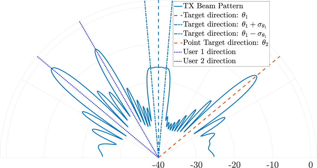
(b) TX beam pattern for high rate requirements.

Figure 2: TX beam patterns for different rate requirements. The DL users locations are $\phi_{1}=-30^{\circ},\phi_{2}=-50^{\circ}$, while the targets locations are $(\theta_{1}=0^{\circ},\sigma_{\theta_{1}}=5^{\circ})$ and $(\theta_{2}=50^{\circ},\sigma_{\theta_{2}}=0^{\circ})$ (point target). For low data rate, we choose $\gamma_{u}=1\,$bps/Hz $\forall u\in\mathcal{L}$, while for high data rate requirements, we choose $\gamma_{u}=7\,$bps/Hz $\forall u\in\mathcal{L}$. The SNR level is $35\,$dB and we assume $N_{b}=M_{b}=32$.

In Fig. 2, we present the designed TX beam pattern we obtain after solving the proposed optimization problem in (34). For the low-rate requirements in Fig. 2(a), we see that most of the transmit power is focused toward the sensing targets. Moreover, we can note that for a target with a large angular spread, the transmit energy is evenly distributed throughout the angular domain occupied by the corresponding target, while for the point target ($\theta_{1}=50^{\circ}$), we notice only a narrow transmit beam lobe. In contrast to this, in Fig. 2(b), as we increase the rate requirements, we note that most of the energy is now focused toward the users to fulfill the rate requirements. Nevertheless, in both cases, we can verify that our proposed algorithm is able to illuminate multiple targets with a wide variety of angular spreads while also fulfilling data rate requirements of DL users.

Figure 3: RMSE of the mean distance and range spread vs $\mathrm{SNR}$.

In Fig. 3, we present the $\mathrm{RMSE}$ of mean distance $d$ and range spread $\sigma_{d}$ against SNR for $\gamma_{u}=0.001\,$bps/Hz $\forall u\in\{1,2,3\}$. It is evident that in the low SNR regime, a high value of range threshold $\eta$ provides a better estimate, while at high SNR, having a low threshold is preferable. This makes sense as in low SNR the signal value is comparable to the noise level, and hence having a low threshold at low SNR will deteriorate the performance. Conversely, in high SNR, since the noise level is negligible, having a low threshold will include maximum signal power without including any noisy signal for range estimation and hence improving the accuracy. In addition to that, we observe that the error in mean range estimation $d$ becomes negligible ($0.7$ meters) at SNR of $20\,$dB, while for $\sigma_{d}$ error gets saturated at around $0.3\,$m at the SNR of $20\,$dB and beyond. This shows that the proposed algorithm achieves high precision for the SNR of $15\,$dB, and beyond.

For angular parameters estimation, we compare the performance of our estimators (TMS defined in (16), and TMS-approx defined in (20)) with the baseline CMS or DISPARE [17] scheme. We also formulate the CMS-approx version of the algorithm as well. For CMS, we use $\mathbf{E}_{s}(\theta,\sigma_{\theta})=\frac{\mathbf{J}(\theta,\sigma_{\theta})}{\left\lvert\left\lvert\mathbf{J}(\theta,\sigma_{\theta})\right\rvert\right\rvert_{\mathrm{F}}}$, while for CMS-approx, we use $\mathbf{E}_{s}^{\mathrm{app}}(\theta,\sigma_{\theta})=\frac{\mathbf{J}_{\mathrm{app}}(\theta,\sigma_{\theta})\mathbf{R}_{\mathbf{X}}\mathbf{J}_{\mathrm{app}}^{\mathrm{H}}(\theta,\sigma_{\theta})}{\left\lvert\left\lvert\mathbf{J}_{\mathrm{app}}(\theta,\sigma_{\theta})\mathbf{R}_{\mathbf{X}}\mathbf{J}_{\mathrm{app}}^{\mathrm{H}}(\theta,\sigma_{\theta})\right\rvert\right\rvert_{\mathrm{F}}}$.

(a) Baseline CMS spectrum.

(b) Baseline CMS-approx spectrum.

(c) Proposed TMS spectrum.

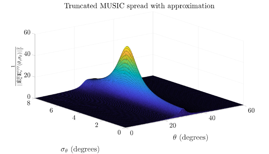
(d) Proposed TMS-approx spectrum.

Figure 4: Spectrum for different versions of MUSIC spread. True parameters of the target are $\theta=30^{\circ}$ and $\sigma_{\theta}=5^{\circ}$ with $\mathrm{SNR}$ value of $30\,$dB.

In Fig. 4, we plot spectra of different MUSIC spread algorithms where we choose $\chi=0.9$. We note that for both CMS and CMS-approx, we get multiple peaks, and the peak at the true parameter values is not a global peak in the spectrum. For instance, the global maximum occurs at $(\hat{\theta}_{\text{\lx@glossaries@gls@link{acronym}{CMS}{{{}}CMS}}},\hat{\sigma}_{\theta,\text{\lx@glossaries@gls@link{acronym}{CMS}{{{}}CMS}}})$ = $(33.2^{\circ},2.5^{\circ})$ and $(\hat{\theta}_{\text{\lx@glossaries@gls@link{acronym}{CMS}{{{}}CMS}-approx}},\hat{\sigma}_{\theta,\text{\lx@glossaries@gls@link{acronym}{CMS}{{{}}CMS}-approx}})$ = $(34^{\circ},2.3^{\circ})$. This is in contrast to both TMS and TMS-approx, where we get a single maxima which is indeed occurring at the neighborhood of true parameters with negligible error, i.e., for TMS and TMS-approx schemes we get peaks at $(\hat{\theta}_{\text{\lx@glossaries@gls@link{acronym}{TMS}{{{}}TMS}}},\hat{\sigma}_{\theta,\text{\lx@glossaries@gls@link{acronym}{TMS}{{{}}TMS}}})$ = $(29.7^{\circ},5.3^{\circ})$ and $(\hat{\theta}_{\text{\lx@glossaries@gls@link{acronym}{TMS}{{{}}TMS}-approx}},\hat{\sigma}_{\theta,\text{\lx@glossaries@gls@link{acronym}{TMS}{{{}}TMS}-approx}})$ = $(29.8^{\circ},5^{\circ})$. This proves that CMS or DISPARE algorithms are susceptible to biases in the spectrum, while in the proposed TMS algorithms, we don’t have this problem.

(a) RMSE ($\theta$) vs SNR for different MUSIC algorithms, where we assume $\gamma_{u}=0.001\,$bps/Hz for all users and $\chi=0.95$.

(b) RMSE ($\theta$) and RMSE ($\sigma_{\theta}$) vs $\sigma_{\theta}$, where we assume $\gamma_{u}=1\,$bps/Hz for all users and SNR = $40\,$dB.

Figure 5: Performance of proposed angle parameters estimation algorithms against baseline schemes.

In Fig. 5(a), we investigate the performance of both proposed algorithms, i.e., TMS and TMS-approx, and compare the RMSE of $\theta$ and $\sigma_{\theta}$ against CMS or DISPARE and CMS-approx. We notice that in the low SNR regime, baseline schemes provide better estimates. This is due to the fact that both baseline schemes try to minimize the weighted subspace fitting, which is beneficial when the SNR is low, i.e., it is better to give more weightage to the eigenvector corresponding to the highest eigenvalue. On the other hand, the proposed algorithm provides a constant weightage to all the eigen vectors of the signal subspace. This affects the performance in the low SNR regime, when the threshold $\chi$ is high. In other words, we noted that choosing a low threshold $\chi$ in the low SNR regime provides better performance in terms of RMSE for both $\theta$ and $\sigma_{\theta}$. Moreover, the figure illustrates that for all the values of SNR TMS-approx provides better performance than the TMS algorithm. This shows that TMS-approx is not only computationally efficient, but also provides us with better estimates. We also see that RMSE performance for both CMS and CMS-approx gets slightly worse with increasing SNR. We speculate this is due to the fact that, as mentioned earlier, CMS algorithms give a bias in the estimate due to the residual term mentioned in (14). This bias can become more consistent in the high SNR regime.

In Fig. 5(b), the effect of $\sigma_{\theta}$ on the performance of TMS-approx and CMS-approx is demonstrated. For this result, we choose $\chi=0.99$. As shown in the figure, the proposed TMS-approx provides better error performance for both $\theta$ and $\sigma_{\theta}$ for the whole range of $\sigma_{\theta}$. In particular, in low $\sigma_{\theta}$ regime (for $\sigma_{\theta}<1^{\circ}$), difference between the performance of TMS-approx and CMS-approx is negligible for both $\theta$ and $\sigma_{\theta}$. However, with increasing $\sigma_{\theta}$, CMS-approx gets worse more rapidly than TMS-approx algorithm. This shows that with increasing $\sigma_{\theta}$, the bias term becomes worse in both $\theta$ and $\sigma_{\theta}$ parameter domains. In addition to that, it is evident that for all the values of $\sigma_{\theta}$, RMSE ($\sigma_{\theta}$) is less than $1^{\circ}$, while RMSE ($\theta$) is less than $2^{\circ}$. On the other hand, the performance of CMS-approx is much worse.

VI Conclusion

This work focuses on the ISAC system with computationally efficient CR target modeling. In particular, we assume that each target has some angular (with mean direction and angular spread) as well as range (with mean range and range spread) densities. To estimate these distribution parameters, we propose algorithms based on TMS (for angular parameters) and DFT (for range parameters). We also propose a fast dynamic beam pattern synthesis algorithm that adapts to different angular spread requirements subject to users’ data rate constraints. The numerical results demonstrate that the proposed algorithms achieve performance superior to that of the baseline scheme in different simulation settings.

References

- [1] 3GPP. Technical Specification Group (TSG). , “Feasibility Study on Integrated Sensing and Communication (Release 19),” 2024.
- [2] ETSI. Group Report (GR) Integrated Sensing And Communications (ISG). , “Integrated Sensing And Communications (ISAC); Use Cases and Deployment Scenarios ,” tech. rep., 2025.
- [3] F. Liu et al., “Integrated sensing and communications: Toward dual-functional wireless networks for 6g and beyond,” IEEE Journal on Selected Areas in Communications, vol. 40, no. 6, pp. 1728–1767, 2022.
- [4] A. Liu, Z. Huang, et al., “A survey on fundamental limits of integrated sensing and communication,” IEEE Communications Surveys & Tutorials, vol. 24, no. 2, pp. 994–1034, 2022.
- [5] C. Sahin et al., “A novel approach for embedding communication symbols into physical radar waveforms,” in 2017 IEEE Radar Conference (RadarConf), pp. 1498–1503, 2017.
- [6] T. Huang, N. Shlezinger, X. Xu, Y. Liu, and Y. C. Eldar, “Majorcom: A dual-function radar communication system using index modulation,” IEEE Transactions on Signal Processing, vol. 68, pp. 3423–3438, 2020.
- [7] C. B. Barneto et al., “Beamformer design and optimization for joint communication and full-duplex sensing at mm-waves,” IEEE Transactions on Communications, vol. 70, no. 12, pp. 8298–8312, 2022.
- [8] H. Hua, J. Xu, and T. X. Han, “Optimal transmit beamforming for integrated sensing and communication,” IEEE Transactions on Vehicular Technology, vol. 72, no. 8, pp. 10588–10603, 2023.
- [9] Z. Liu, S. Aditya, H. Li, and B. Clerckx, “Joint transmit and receive beamforming design in full-duplex integrated sensing and communications,” IEEE Journal on Selected Areas in Communications, vol. 41, no. 9, pp. 2907–2919, 2023.
- [10] M. Talha, B. Smida, M. A. Islam, and G. C. Alexandropoulos, “Multi-target two-way integrated sensing and communications with full duplex mimo radios,” in 2023 57th Asilomar Conference on Signals, Systems, and Computers, pp. 1661–1667, 2023.
- [11] M. A. Islam, G. C. Alexandropoulos, and B. Smida, “Integrated sensing and communication with millimeter wave full duplex hybrid beamforming,” in ICC 2022 - IEEE International Conference on Communications, pp. 4673–4678, 2022.
- [12] Z. Du et al., “Integrated sensing and communications for V2I networks: Dynamic predictive beamforming for extended vehicle targets,” IEEE Transactions on Wireless Communications, vol. 22, no. 6, pp. 3612–3627, 2023.
- [13] F. Liu et al., “Cramér-rao bound optimization for joint radar-communication beamforming,” IEEE Transactions on Signal Processing, vol. 70, pp. 240–253, 2022.
- [14] N. Garcia et al., “Cramér-rao bound analysis of radars for extended vehicular targets with known and unknown shape,” IEEE Transactions on Signal Processing, vol. 70, pp. 3280–3295, 2022.
- [15] Y. Wang, M. Tao, S. Sun, and W. Cao, “Cramér-rao bound analysis and beamforming design for 3D extended target in ISAC,” in GLOBECOM 2024 - 2024 IEEE Global Communications Conference, pp. 5344–5349, 2024.
- [16] 3GPP, Group Radio Access Network, “TR 38.901: Study on channel model for frequencies from 0.5 to 100 GHz,” jan 2020. Release 16, v16.1.0.
- [17] Y. Meng et al., “Estimation of the directions of arrival of spatially dispersed signals in array processing,” IEE Proceedings - Radar, Sonar and Navigation, vol. 143, pp. 1–9, 1996.
- [18] S. Valaee, B. Champagne, and P. Kabal, “Parametric localization of distributed sources,” IEEE Transactions on Signal Processing, vol. 43, no. 9, pp. 2144–2153, 1995.
- [19] M. Bengtsson and B. Ottersten, “A generalization of weighted subspace fitting to full-rank models,” IEEE Transactions on Signal Processing, vol. 49, no. 5, pp. 1002–1012, 2001.
- [20] E. Björnson, M. Bengtsson, and B. Ottersten, “Optimal multiuser transmit beamforming: A difficult problem with a simple solution structure [lecture notes],” IEEE Signal Processing Magazine, vol. 31, no. 4, pp. 142–148, 2014.
- [21] A. Wiesel, Y. Eldar, and S. Shamai, “Linear precoding via conic optimization for fixed mimo receivers,” IEEE Transactions on Signal Processing, vol. 54, no. 1, pp. 161–176, 2006.