DiffEM: Learning from Corrupted Data with Diffusion Models via Expectation Maximization

Abstract

Diffusion models have emerged as powerful generative priors for high-dimensional inverse problems, yet learning them when only corrupted or noisy observations are available remains challenging. In this work, we propose a new method for training diffusion models with Expectation-Maximization (EM) from corrupted data. Our proposed method, DiffEM, utilizes conditional diffusion models to reconstruct clean data from observations in the E-step, and then uses the reconstructed data to refine the conditional diffusion model in the M-step. Theoretically, we provide monotonic convergence guarantees for the DiffEM iteration, assuming appropriate statistical conditions. We demonstrate the effectiveness of our approach through experiments on various image reconstruction tasks.

1 Introduction

Diffusion models (Song and Ermon, 2019; Ho et al., 2020; Song et al., 2020) have emerged as powerful tools for learning high-dimensional distributions, achieving remarkable success across a broad range of generative tasks. Their effectiveness as learned priors has led to significant advances in solving inverse problems (Kawar et al., 2021; Choi et al., 2021; Saharia et al., 2022), including image inpainting, denoising, and super-resolution. However, in many real-world scenarios, acquiring clean training data remains difficult or costly, and can raise significant concerns, as training on clean data might lead to memorization (Somepalli et al., 2023a; Carlini et al., 2023; Somepalli et al., 2023b; Shah et al., 2025), posing privacy and copyright risks. While data with mild or moderate corruption is often more readily available, particularly in domains like medical imaging (Wang et al., 2016; Zbontar et al., 2018) and compressive sensing, training diffusion models effectively using only corrupted or noisy observations presents substantial technical challenges.

The fundamental difficulty lies in the fact that standard techniques for training diffusion models are designed for settings with access to clean data from the prior distribution. When only corrupted or noisy observations are available, these techniques become inapplicable, and training diffusion models effectively reduces to learning a latent variable model from corrupted observations, a problem well-known for its theoretical and practical challenges.

Recent work (Rozet et al., 2024; Bai et al., 2024) has proposed addressing this challenge by applying the Expectation-Maximization (EM) method with diffusion models as priors. However, this approach faces a critical difficulty: in each E-step, the algorithm must sample from the posterior distribution given the corrupted observations, whereas it only has access to the score function of the diffusion prior. To overcome this, these works adopt ad hoc posterior sampling schemes that rely on various approximations of the posterior score function that explicitly incorporate the corruption process. Such approximation schemes, however, are based on implicit structural assumptions about the true prior and the corruption process, making their approximation errors difficult to quantify.

In this work, we propose a new method that combines diffusion models with the EM framework. Our key insight is that instead of learning a diffusion prior and then performing approximate sampling, we can directly model the posterior distribution using a conditional diffusion model (Saharia et al., 2022; Daras et al., 2024a). The primary advantage of our approach is its independence from specific approximate posterior sampling schemes. Notably, it can handle any corruption channel, as it makes no assumptions about the prior and corruption channel beyond requiring that the posterior score function can be expressed by the denoiser network. Furthermore, we provide theoretical analysis of the proposed EM iteration, demonstrating its convergence under appropriate conditions on the approximation error of the denoiser network. We validate our approach through extensive experiments on both synthetic and real-world datasets with various types of corruption, including low-dimensional manifold learning and image reconstruction on CIFAR-10 and CelebA.

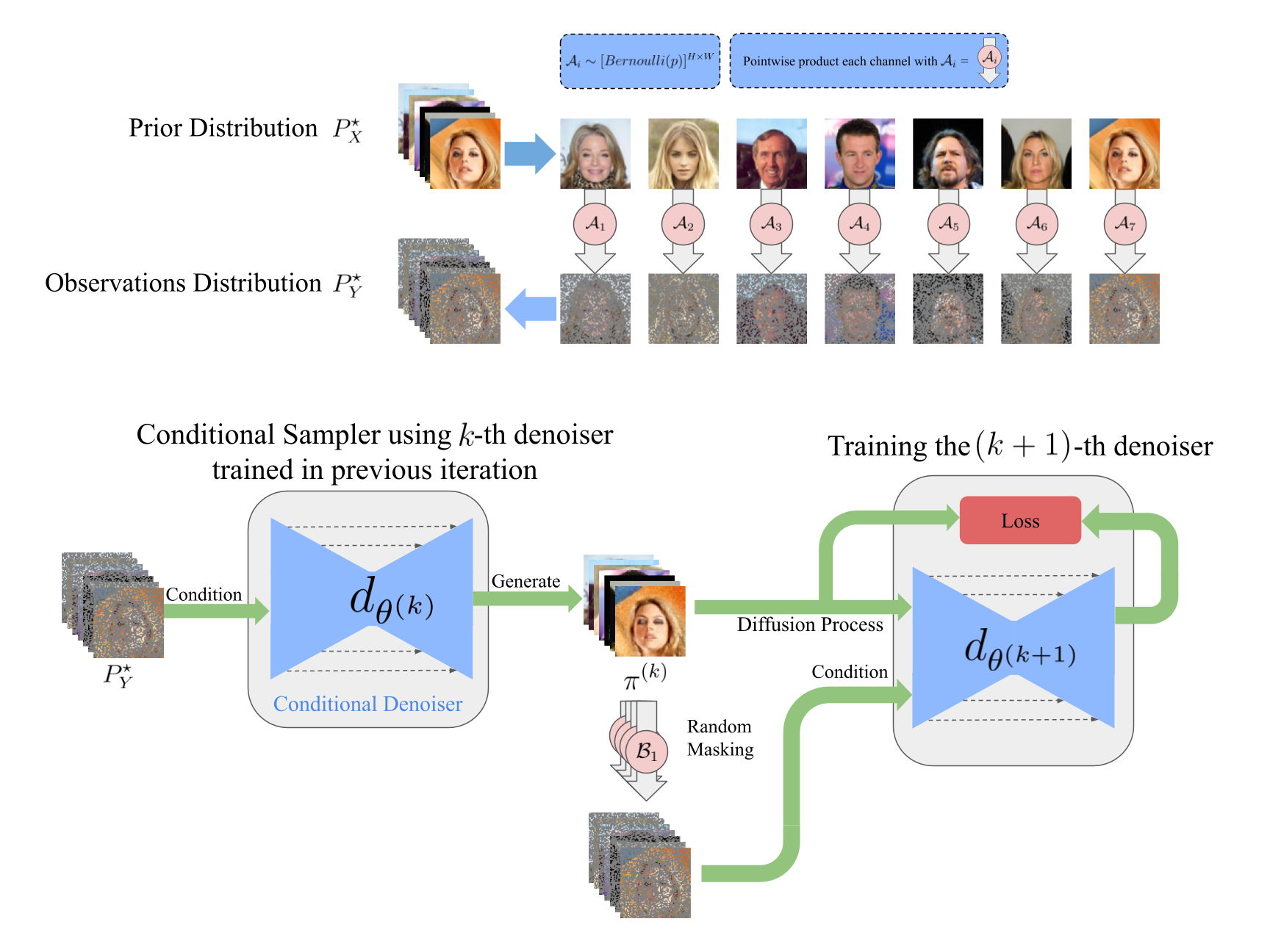
Figure 1: Top: Illustration of a single DiffEM iteration, where the conditional denoiser $d_{\theta^{(k)}}$ (trained in the previous iteration) generates reconstructed images during the E-step, and the next denoiser $d_{\theta^{(k+1)}}$ is trained on the reconstructed dataset during the M-step via the diffusion process and conditional score matching loss.

1.1 Preliminaries

Problem setup

Formally, we consider the following setup. The prior $P_{X}^{\star}$ is a distribution over the space $\mathcal{X}$ of latent variables. The forward channel (or corruption process) $\mathbf{Q}(\cdot|X)$ maps each point $X\in\mathcal{X}$ to a distribution over the observation space $\mathcal{Y}$. The observation is generated as

$$\addcontentsline{lla}{section}{\numberline{\string\crtrefnumber{eq:Y-dist}}{e}q:Y-dist}Y\sim\mathbf{Q}(\cdot|X),\quad\text{where }X\sim P_{X}^{\star},$$ (1)

and we denote $P^{\star}$ to be the joint distribution of $(X,Y)$ and $P_{Y}^{\star}$ to be the marginal distribution of $Y$. This formulation encompasses classical inverse problems, which arise from a forward channel of the form $\mathbf{Q}(\cdot|X)=\mathsf{N}{\left(\mathcal{A}(X),\sigma_{Y}^{2}\mathbf{I}\right)}$ where $\mathcal{A}:\mathcal{X}\to\mathbb{R}^{d_{y}}$ is a known forward operator.

In our setting, the learner only has access to a dataset $\{Y^{[1]},\cdots,Y^{[N]}\}$ consisting of i.i.d. observations from $P_{Y}^{\star}$. The forward channel $\mathbf{Q}$ is also known. The goal is two-fold:

• Prior reconstruction: to generate new samples from the ground-truth prior $P_{X}^{\star}$ approximately.

• Posterior sampling: to sample $X\sim P^{\star}(\cdot|Y)$ given an observation $Y$.

With this setup, the primary focus of recent work (Daras et al., 2023b, a; Rozet et al., 2024; Bai et al., 2024; Daras et al., 2024b) has been on prior reconstruction under the linear corruption process. In such settings, the latent space is $\mathcal{X}=\mathbb{R}^{{d_{x}}}$ (consisting of “clean images”), and there is a known distribution $P_{A}$ of corruption matrices $A\in\mathbb{R}^{{d_{y}}\times{d_{x}}}$. The observation is drawn as

$$\addcontentsline{lla}{section}{\numberline{\string\crtrefnumber{eq:linear-corr}}{e}q:linear-corr}Y=(AX+\epsilon,A),\quad\text{where }X\sim P_{X}^{\star},A\sim P_{A},\epsilon\sim\mathsf{N}{\left(0,\sigma_{Y}^{2}\mathbf{I}\right)},$$ (2)

i.e., the observation $Y$ is a (corrupted image, corruption matrix) pair, with the image corrupted by the matrix $A\sim P_{A}$ and the additive Gaussian noise $\epsilon$. By choosing different distributions $P_{A}$ for the corruption matrix, the linear corruption process (2) can model problems including random masking (Daras et al., 2023b; Rozet et al., 2024; Bai et al., 2024) and blurring (Bai et al., 2024).

Diffusion models

Given samples from a data distribution $p_{0}$ over $\mathbb{R}^{d}$, diffusion models aim to learn how to generate new samples from $p_{0}$. Following Song et al. (2020), we consider the diffusion process $(X_{t})_{t\in[0,1]}$ with $X_{0}\sim p_{0}$, and $X_{t}|X_{0}\sim\mathsf{N}{\left(X_{0},\sigma_{t}^{2}\mathbf{I}\right)}$. Formally, the diffusion process can be described by the following stochastic differential equation (SDE):

$$\addcontentsline{lla}{section}{\numberline{\string\crtrefnumber{eqn:diffusion-process}}{e}qn:diffusion-process}\mathrm{d}X_{t}=g(t)\mathrm{d}\mathbf{B}_{t},\qquad X_{0}\sim p_{0},$$ (3)

where $g(t)^{2}=\frac{d\sigma_{t}^{2}}{dt}$, and $(\mathbf{B}_{t})_{t\in[0,1]}$ is the standard Brownian motion. Let $p_{t}(x)$ be the density function of $X_{t}\in\mathbb{R}^{d}$. It is well-known that the reverse of process (3) can be described by the following reverse-time diffusion process:

$$\addcontentsline{lla}{section}{\numberline{\string\crtrefnumber{eqn:diffusion-process-reverse}}{e}qn:diffusion-process-reverse}\mathrm{d}X_{t}=-g(t)^{2}\nabla_{x}p_{t}(X_{t})\mathrm{d}t+g(t)\mathrm{d}\mathbf{B}_{t},\qquad X_{1}\sim p_{1}.$$ (4)

With $\sigma_{1}$ being sufficiently large, we have $p_{1}\approx\mathsf{N}{\left(0,\sigma_{1}^{2}\mathbf{I}\right)}$. The score function $(x,t)\mapsto\nabla_{x}\log p_{t}(x)$ is typically parametrized by a neural network $\mathbf{s}_{\theta}(x,t)$. By Tweedie’s formula, $\nabla_{x}\log p_{t}(x)=\frac{\mathbb{E}[X_{0}|X_{t}=x]-x}{\sigma_{t}^{2}}$, where the expectation is taken with respect to the diffusion process (3). Hence, $\mathbf{s}_{\theta}(x,t)$ can be learned by optimizing the score-matching loss.

1.2 Related work

Learning diffusion models with corrupted datasets

Recent advances in diffusion models (Ho et al., 2020; Song et al., 2020) have demonstrated remarkable success in learning high-dimensional distributions. However, training diffusion models with corrupted data presents significant challenges, as most existing techniques are designed for clean datasets, and learning latent variable models is known to be theoretically and practically difficult. Several approaches have been proposed to address this challenge using diffusion models. For linear corruption $Y\sim\mathsf{N}{\left(AX,\sigma_{Y}^{2}\mathbf{I}\right)}$ (cf. Eq. (2)), methods such as SURE-score (Aali et al., 2023), GSURE (Kawar et al., 2023), and Ambient-Diffusion (Daras et al., 2023b; Aali et al., 2025; Daras et al., 2025) train the denoiser network using a surrogate loss function. Specializing to Gaussian corruption $Y\sim\mathsf{N}{\left(X,\sigma_{Y}^{2}\mathbf{I}\right)}$, Daras et al. (2023a, 2024b) propose enforcing consistency of the diffusion model to enable generalization to unseen noise levels, while Lu et al. (2025) develop an iterative scheme to refine the diffusion prior. Recent work (Rozet et al., 2024; Bai et al., 2024) identifies the Expectation-Maximization (EM) method as a promising framework for training diffusion priors with linearly corrupted observations. However, as these EM approaches employ diffusion models as priors, they rely heavily on approximation schemes for posterior sampling (detailed discussion in Section˜2.1).

Solving inverse problems with diffusion models

Diffusion models have also been shown as powerful priors for a wide range of inverse problems in computer vision and medical imaging. A line of work—including SNIPS (Kawar et al., 2021), ILVR (Choi et al., 2021), DDRM (Kawar et al., 2022), Palette (Saharia et al., 2022), and DPS (Chung et al., 2022), among others—has demonstrated the effectiveness of both unconditional and conditional diffusion models in addressing various tasks, such as super-resolution, inpainting, deblurring, and compressed sensing. As surveyed by Daras et al. (2024a), many of these approaches leverage learned diffusion priors and perform posterior sampling through approximations of the posterior score function, and the previous work on EM (Rozet et al., 2024; Bai et al., 2024) also follows this approach.

2 Expectation-Maximization Approach

For a class of parameterized latent variable models $\{q_{\theta}(x,y)\}_{\theta}$ where $x$ is the value of the latent variable and $y$ is that of the observable one, the Expectation-Maximization (EM) method aims to find a parameter $\theta$ that maximizes the population log-likelihood of the observable variable, where $q_{\theta}(y)$ below refers to the marginal of model $q_{\theta}(x,y)$ with respect to the observable variable:

$$\max_{\theta}\mathcal{L}(\theta)\mathrel{\mathop{:}}=\mathbb{E}_{Y\sim P_{Y}^{\star}}\log q_{\theta}(Y).$$

This optimization problem is equivalent to minimizing the KL divergence between $P_{Y}^{\star}$ and $q_{\theta}(y)$. However, direct optimization is computationally intractable for most problems. To overcome this computational challenge, each step of the EM method optimizes the following ELBO lower bound with a parameter ${\widehat{\theta}}$:

$$\mathcal{L}(\theta)\geq\mathbb{E}_{Y\sim P_{Y}^{\star}}\mathbb{E}_{X\sim q_{\widehat{\theta}}(X|Y)}\log\frac{q_{\theta}(X,Y)}{q_{\widehat{\theta}}(X|Y)}.$$

In particular, the EM algorithm can be succinctly written as: Starting from an initial point $\theta^{(0)}$, iterate

$$\theta^{\scriptscriptstyle(k+1)}=\operatorname*{arg\,max}_{\theta}\mathbb{E}_{Y\sim P_{Y}^{\star}}\mathbb{E}_{X\sim q_{\theta^{\scriptscriptstyle(k)}}(X|Y)}\log q_{\theta}(X,Y).$$

In our setting, since the forward channel $\mathbf{Q}$ is known and simple, the parametrized model should satisfy $q_{\theta}(x,y)=\mathbf{Q}(Y=y|X=x)q_{\theta}(x)$. In this case, the EM iterations reduce to

$$\addcontentsline{lla}{section}{\numberline{\string\crtrefnumber{eq:latent-EM}}{e}q:latent-EM}\theta^{\scriptscriptstyle(k+1)}=\operatorname*{arg\,max}_{\theta}\mathbb{E}_{Y\sim P_{Y}^{\star}}\mathbb{E}_{X\sim q_{\theta^{\scriptscriptstyle(k)}}(X|Y)}\log q_{\theta}(X).$$ (5)

This specialization of EM has been studied in (Aubin-Frankowski et al., 2022; Rozet et al., 2024; Bai et al., 2024), and it is also the basis of our framework. To simplify the notation, we consider the mixture posterior distribution $\pi^{\scriptscriptstyle(k)}$ with density $\pi^{\scriptscriptstyle(k)}(x)=\mathbb{E}_{Y\sim P_{Y}^{\star}}{\left[q_{\theta^{\scriptscriptstyle(k)}}(x|Y)\right]}$, which is a mixture with respect to the observation distribution $P_{Y}^{\star}$ of the posteriors $q_{\theta^{\scriptscriptstyle(k)}}(X|Y)$  (Rozet et al., 2024). Then, the EM update (5) can be rewritten as

$$\addcontentsline{lla}{section}{\numberline{\string\crtrefnumber{eq:latent-EM-prior}}{e}q:latent-EM-prior}\theta^{\scriptscriptstyle(k+1)}=\operatorname*{arg\,min}_{\theta}D_{\mathrm{KL}}(\pi^{\scriptscriptstyle(k)}(x)\;\|\;q_{\theta}(x)),$$ (6)

i.e., the model $q_{\theta^{\scriptscriptstyle(k+1)}}$ minimizes the distance to the mixture posterior distribution $\pi^{\scriptscriptstyle(k)}$. Crucially, to implement this update, we need to be able to sample from the conditional distribution $q_{\theta^{\scriptscriptstyle(k)}}(X|Y)$.

2.1 Prior approach: EM with diffusion priors

In this section, we briefly review how prior work (Rozet et al., 2024; Bai et al., 2024) performs posterior sampling with diffusion models as priors. Their methods are restricted to the linear corruption model Eq.˜2, where the observation is $Y=(AX+\epsilon,A)$, where $\epsilon\sim\mathsf{N}{\left(0,\sigma_{Y}^{2}\mathbf{I}\right)}$ is the noise and $A\sim P_{A}$ is a random corruption matrix. For simplicity, to describe these results, we focus on the case where $A$ is fixed, i.e. the forward channel is $\mathbf{Q}(\cdot|X)=\mathsf{N}{\left(AX,\sigma_{Y}^{2}\mathbf{I}\right)}$.

In the EM approach of Rozet et al. (2024); Bai et al. (2024), the latent variable models are described by diffusion models. More precisely, each $\theta$ parametrizes a score function $\mathbf{s}_{\theta}(x,t)$, and $q_{\theta}(x)$ corresponds to the distribution of $X_{0}$ obtained by running the backward diffusion process with the score function $\mathbf{s}_{\theta}$. However, to sample from $q_{\theta}(X|Y)$, one needs to approximate the conditional score function $\nabla_{x}\log q_{\theta}(X_{t}=x|Y=y)$. Following previous work on posterior sampling with diffusion priors (Chung et al., 2022, etc.), the conditional score is decomposed according to Bayes’ rule:

$$\nabla_{x}\log q_{\theta}(X_{t}=x|Y)=\nabla_{x}\log q_{\theta}(Y|X_{t}=x)+\nabla_{x}\log q_{\theta}(X_{t}=x).$$

The second term is given by the score function $\mathbf{s}_{\theta}(x,t)$. To approximate the first term, Rozet et al. (2024) applies a Gaussian approximation $q_{\theta}(X=\cdot|X_{t}=x)\approx\mathsf{N}{\left(\mathbb{E}_{\theta}[X|X_{t}=x],\mathbb{V}_{\theta}[X|X_{t}=x]\right)}$. Consequently, the conditional distribution of $Y$ is approximately

$$q_{\theta}(Y=\cdot|X_{t}=x)\approx\mathsf{N}{\left(A\mathbb{E}_{\theta}[X|X_{t}=x],\sigma_{Y}^{2}\mathbf{I}+A\mathbb{V}_{\theta}[X|X_{t}=x]A^{\top}\right)}.$$

Then, to calculate $\nabla_{x}\log q_{\theta}(Y|X_{t}=x)$, Rozet et al. (2024) introduces moment matching techniques to approximate the variance function $\mathbb{V}_{\theta}[X|X_{t}=x]$. Alternatively, Bai et al. (2024) applies a simpler approximation $q_{\theta}(Y=\cdot|X_{t}=x)\approx\mathsf{N}{\left(A\mathbb{E}_{\theta}[X|X_{t}=x],\sigma_{Y}^{2}\mathbf{I}\right)}$.

However, these approximations all rely on the assumption that $q_{\theta}(X_{0}=\cdot|X_{t}=x)$ is close to a Gaussian distribution. This assumption may not hold for general diffusion priors, which are highly multi-modal. Therefore, errors in these approximation schemes can be difficult to control. Furthermore, even when the learned diffusion prior $q_{\theta}$ is close to the ground truth, the posterior distribution of $X|Y$ (obtained by approximating the score $\nabla_{x}\log q_{\theta}(X_{t}=x|Y)$) might not accurately represent the true conditional distribution $q_{\theta}(X|Y)$ under the diffusion prior $q_{\theta}(X)$.

Additionally, the moment matching techniques of Rozet et al. (2024) are rather sophisticated and specialized to the linear corruption process. For general forward channels with non-linear transformations, calculating the score $\nabla_{x}\log q_{\theta}(Y|X_{t}=x)$ can be challenging even under the Gaussian approximation assumption.

2.2 Our Approach: EM with conditional diffusion model

Instead of parametrizing the prior distribution $q_{\theta}(x)$ using a diffusion model, we directly model the posterior distribution $q_{\theta}(x|y)$ through a conditional score function network $\mathbf{s}_{\theta}(x,t|y)$. Below, we describe the corresponding conditional diffusion process for generating posterior samples.

Conditional diffusion process

Given a latent variable model $q$, we consider the diffusion process

$$\addcontentsline{lla}{section}{\numberline{\string\crtrefnumber{eqn:cond-diffusion-process}}{e}qn:cond-diffusion-process}(X_{0},Y)\sim q,\qquad\mathrm{d}X_{t}=g(t)\mathrm{d}\mathbf{B}_{t}.$$ (7)

Let $p$ be the joint distribution of $(\left\{X_{t}\right\}_{t\in[0,1]},Y)$. To sample from $q(X_{0}|Y)$, we consider the following reverse-time process:

$$\addcontentsline{lla}{section}{\numberline{\string\crtrefnumber{eqn:cond-diffusion-process-rev}}{e}qn:cond-diffusion-process-rev}\mathrm{d}X_{t}=-g(t)^{2}\mathbf{s}_{\theta}(X_{t},t|Y)\mathrm{d}t+g(t)\mathrm{d}\mathbf{B}_{t},\qquad X_{1}\sim q_{1}(\cdot|Y),$$ (8)

where the network $\mathbf{s}_{\theta}$ directly approximates the true conditional score function

$$\mathbf{s}_{\theta}(x,t|y)\approx\nabla_{x}\log p(X_{t}=x|y)=\frac{\mathbb{E}\left[X_{0}\left|X_{t}=x,Y=y\right.\!\right]-x}{\sigma_{t}^{2}},$$ (9)

and the expectation is taken over the process (7) (see e.g. (Daras et al., 2024a)). For a given parameter $\theta$ that parameterizes the conditional denoiser network $\mathbf{s}_{\theta}$, we let $q_{\theta}(X=\cdot|Y)$ be the distribution of $X_{0}$ generated by Eq.˜8. In particular, when $\mathbf{s}_{\theta}(x,t|y)=\nabla_{x}\log p(X_{t}=x|y)$, the reverse process (8) indeed generates $X_{0}\sim q(\cdot|Y)$, i.e., $q_{\theta}(\cdot|Y)=q(\cdot|Y)$.

EM with conditional diffusion models

Based on the conditional diffusion process, we propose the EM procedure Algorithm˜1, using a conditional diffusion model to learn the posterior directly.

0: Dataset of corrupted observations $\mathcal{D}_{Y}=\left\{Y^{[1]},\cdots,Y^{[N]}\right\}$, a known forward channel $\mathbf{Q}(\cdot|X)$, and a initialization for the conditional model $\theta^{\scriptscriptstyle(0)}$.

 for $k=0,1,\cdots,K-1$ do

  // E-step:

  for $i\in[N]$ do

   Generate the reconstruction $X^{[i]}\sim q_{\theta^{\scriptscriptstyle(k)}}(\cdot|Y^{[i]})$ using the current conditional model $\theta^{\scriptscriptstyle(k)}$.

  // M-step:

  Train a new conditional diffusion model using the dataset $\mathcal{D}^{\scriptscriptstyle(k)}_{X}=\{X^{[1]},\cdots,X^{[N]}\}$ and the forward model $\mathbf{Q}(\cdot|X)$ by minimizing the objective provided in Eq.˜10:

$$\theta^{\scriptscriptstyle(k+1)}=\operatorname*{arg\,min}_{\theta}L_{\mathrm{SM},k}(\theta).$$

 (1) The conditional diffusion model $\theta^{\scriptscriptstyle(K)}$, and

 (2) An unconditional diffusion model $\widehat{\theta}$ trained on the dataset $\mathcal{D}_{X}^{\scriptscriptstyle(K-1)}$.

Algorithm 1 DiffEM: Expectation-Maximization with a conditional diffusion model

In the E-step, the algorithm generates the dataset $\mathcal{D}_{X}^{\scriptscriptstyle(k)}=\{X^{[1]},\cdots,X^{[N]}\}$ consisting of the reconstruction $X^{[i]}\sim q_{\theta^{\scriptscriptstyle(k)}}(\cdot|Y^{[i]})$. Then, in the M-step, the algorithm uses the dataset $\mathcal{D}_{X}^{\scriptscriptstyle(k)}$ to train the conditional diffusion model $\theta^{\scriptscriptstyle(k+1)}$, so that it learns to sample from $\widehat{P}^{\scriptscriptstyle(k)}(X|Y)$, the posterior of $\widehat{P}^{\scriptscriptstyle(k)}(X,Y)$ which samples $X\sim\mathcal{D}_{X}^{\scriptscriptstyle(k)}$ and then samples $Y\sim\mathbf{Q}(\cdot|X)$. To train this model, we consider the following conditional score matching loss:

$$\addcontentsline{lla}{section}{\numberline{\string\crtrefnumber{def:cond-score-loss}}{d}ef:cond-score-loss}L_{\mathrm{SM},k}(\theta)=\int_{0}^{1}\lambda_{t}\mathbb{E}_{X\sim\mathcal{D}_{X}^{\scriptscriptstyle(k)},Y\sim\mathbf{Q}(\cdot|X)}\mathbb{E}_{X_{t}=X+\sigma_{t}Z}\left\|\mathbf{s}_{\theta}(X_{t},t|Y)+Z\right\|^{2}\mathrm{d}t,$$ (10)

where $Z\sim\mathsf{N}{\left(0,\mathbf{I}\right)}$ is the unit noise, and $\lambda_{t}\geq 0$ is a weight sequence. It is straightforward to verify that, assuming the network $\mathbf{s}_{\theta}$ is expressive enough, the minimizer $\theta^{\star}$ of $L_{\mathrm{SM},k}$ satisfies $\mathbf{s}_{\theta^{\star}}(x,t|y)=\frac{\mathbb{E}\left[X_{0}\left|X_{t}=x,Y=y\right.\!\right]-x}{\sigma_{t}^{2}}$, where the conditional expectation is taken with respect to the distribution sampling variables as $X_{0}\sim\mathcal{D}_{X}^{\scriptscriptstyle(k)}$, $Y\sim\mathbf{Q}(\cdot|X_{0})$, $X_{t}\sim\mathsf{N}{\left(X_{0},\sigma_{t}^{2}\mathbf{I}\right)}$. Therefore, as long as the M-step is done successfully, we expect to have $q_{\theta^{\scriptscriptstyle(k+1)}}(X|Y)\approx\widehat{P}^{\scriptscriptstyle(k)}(X|Y)$ (cf. Section˜3).

The advantage of conditional diffusion model

Unlike approaches that rely on ad hoc approximation schemes for the posterior score function using unconditional diffusion models (Rozet et al., 2024; Bai et al., 2024), our framework directly employs a conditional diffusion model. Both the prior and the corruption channel are implicitly encoded in this model through the minimization of the conditional score matching loss (10). In experiments (Section˜4), we observe that DiffEM consistently outperforms EM methods with diffusion priors. As predicted by our theoretical analysis (Section˜3), this improvement is largely due to the fact that conditional models avoid the approximation bottleneck inherent in heuristic posterior sampling schemes.

Output: Posterior sampler $\theta^{\scriptscriptstyle(K)}$ and diffusion prior $\widehat{\theta}$

Our framework is designed to address two complementary goals: (1) posterior sampling and (2) prior reconstruction (cf. Section˜1.1). The conditional diffusion model trained by DiffEM naturally serves as a posterior sampler. For prior reconstruction, we leverage the reconstructed dataset $\mathcal{D}_{X}^{\scriptscriptstyle(K-1)}$ generated during the final EM iteration, and train an unconditional diffusion prior on this dataset. In particular, when the target application requires only a diffusion prior (Daras et al., 2023b; Rozet et al., 2024; Bai et al., 2024), we may directly use $\widehat{\theta}$. In such cases, the conditional model adopted by our approach primarily serves as a means to accelerate EM convergence.

Computational efficiency of DiffEM

The computational cost of DiffEM can be decomposed as

$$\addcontentsline{lla}{section}{\numberline{\string\crtrefnumber{eq:comp-cost}}{e}q:comp-cost}\text{Total Time}=T_{\sf init}+K\cdot T_{\sf ft}+T_{\sf u},$$ (11)

where $K$ is the number of EM iterations, $T_{\sf init}$ is the time of training a standard conditional diffusion model from scratch, $T_{\sf ft}\leq T_{\sf init}$ is the average time of fine-tuning the conditional diffusion model for each M-step, and $T_{\sf u}$ is the cost of training an unconditional model to output. The cost $T_{\sf init}\geq T_{\sf ft}$ of training diffusion model is intrinsic to diffusion-based learning methods. Thus, DiffEM can be interpreted as increasing the training cost by a multiplicative factor of $K$ (the number of EM iterations), which we view as the unavoidable cost of working with only corrupted data.

In general, the computational cost of EM-based methods (Rozet et al., 2024; Bai et al., 2024) can always be decomposed as Eq.˜11. In our experiments, we compare the computation time $K$, $T_{\sf init}$, and $T_{\sf ft}$ of DiffEM and EM-MMPS in CIFAR-10 experiments (Table˜2).

3 Monotonic Improvement Property and Convergence

In this section, we analyze the convergence properties of the EM iteration. As observed by Aubin-Frankowski et al. (2022), when the iteration (6) is exact, i.e., when the sample size is infinite and the conditional model $q_{\theta^{\scriptscriptstyle(k+1)}}$ learns the mixture posterior exactly in each M-step, the EM iteration is equivalent to mirror descent in the space of measures. Therefore, the convergence of the exact EM iteration follows immediately from the guarantees of mirror descent.

We study the DiffEM iteration, taking the score-matching error introduced by the M-step into account. For simplicity, we analyze the EM iteration with fresh corrupted samples. Specifically, we consider the variant of Algorithm˜1 where, at each iteration $k=0,1,\cdots,K-1$, a new dataset of corrupted observations $\mathcal{D}_{Y}^{\scriptscriptstyle(k)}=\left\{Y^{[1]},\cdots,Y^{[N]}\right\}\sim P_{Y}^{\star}$ is drawn in the E-step. We continue to refer to this procedure as DiffEM throughout this section.

Under this variant, for each $k$, the reconstructed dataset $\mathcal{D}_{X}^{\scriptscriptstyle(k)}=\{X^{[1]},\cdots,X^{[N]}\}$ consists of i.i.d samples from the posterior mixture distribution $\pi^{\scriptscriptstyle(k)}=\mathbb{E}_{Y\sim P_{Y}^{\star}}[q_{\theta^{\scriptscriptstyle(k)}}(\cdot|Y)]$. We let $P^{\scriptscriptstyle(k)}$ be the joint probability distribution of $(X,Y)$ under $X\sim\pi^{\scriptscriptstyle(k)},Y\sim\mathbf{Q}(\cdot|X)$, and write $P_{Y}^{\scriptscriptstyle(k)}$ for the marginal of $Y$. The convergence is measured in terms of $D_{\mathrm{KL}}(P_{Y}^{\star}\;\|\;P_{Y}^{\scriptscriptstyle(k)})$, the Kullback-Leibler (KL) divergence between the true observation distribution $P_{Y}^{\star}$ and the distribution $P_{Y}^{\scriptscriptstyle(k)}$. Intuitively, this measures how plausible the prior $\pi^{\scriptscriptstyle(k)}$ is by comparing the induced observation distribution $P_{Y}^{\scriptscriptstyle(k)}$ to $P_{Y}^{\star}$.

Score-matching error

We define the score-matching error of the $k$th M-step as

$$\varepsilon_{\sf SM}^{\scriptscriptstyle(k)}\mathrel{\mathop{:}}=\mathbb{E}_{Y\sim P_{Y}^{\star}}D_{\mathrm{KL}}(q_{\theta^{\scriptscriptstyle(k+1)}}(\cdot|Y)\;\|\;P^{\scriptscriptstyle(k)}(\cdot|Y)),$$

which measures the KL divergence between the conditional diffusion model $q_{\theta^{\scriptscriptstyle(k+1)}}$ learned in the $k$th M-step and the true posterior $P^{\scriptscriptstyle(k)}(\cdot|Y)$. This error can be decomposed into two components: (1) the error of the learned score function, which is the statistical error of score matching (10) with a finite sample size, and (2) the sampling error, which comes from the discretized backward diffusion process (8) starting from a noisy Gaussian. When the denoiser network is sufficiently expressive, the score matching error can be upper bounded through statistical learning theory (Dou et al., 2024; Zhang et al., 2024; Wibisono et al., 2024; Chen et al., 2024; Gatmiry et al., 2024, etc.). The sampling error is addressed by existing work on backward diffusion sampling (see e.g., Chen et al., 2022; Conforti et al., 2023, 2025)). Therefore, under appropriate conditions, it can be shown that the score-matching error $\varepsilon_{\sf SM}^{\scriptscriptstyle(k)}\to 0$ as the sample size $N$ increases.

Monotonicity of EM

Our first result (shown in Section˜A.1) is the following approximate monotonicity property of the EM iteration in terms of the statistical error $\varepsilon_{\sf SM}^{\scriptscriptstyle(k)}$.

Lemma 1 (Monotonic improvement).

For any $k\geq 0$, it holds that

$$\underbrace{D_{\mathrm{KL}}(P_{Y}^{\star}\;\|\;P_{Y}^{\scriptscriptstyle(k+1)})}_{\text{error of prior $\pi^{\scriptscriptstyle(k+1)}$}}\leq\underbrace{D_{\mathrm{KL}}(P_{Y}^{\star}\;\|\;P_{Y}^{\scriptscriptstyle(k)})}_{\text{error of prior $\pi^{\scriptscriptstyle(k)}$}}-\underbrace{D_{\mathrm{KL}}(\pi^{\scriptscriptstyle(k+1)}\;\|\;\pi^{\scriptscriptstyle(k)})}_{\text{difference between priors}}+\underbrace{\varepsilon_{\sf SM}^{\scriptscriptstyle(k)}}_{\text{score-matching error of }q_{\theta^{\scriptscriptstyle(k+1)}}}.$$

Therefore, when the statistical error $\varepsilon_{\sf SM}^{\scriptscriptstyle(k)}\to 0$, the divergence $D_{\mathrm{KL}}(P_{Y}^{\star}\;\|\;P_{Y}^{\scriptscriptstyle(k)})$ is monotonically decreasing. In other words, in the EM iteration, the observation distribution induced by prior $\pi^{\scriptscriptstyle(k+1)}$ is always closer to $P_{Y}^{\star}$ compared to the observation distribution induced $\pi^{\scriptscriptstyle(k)}$, modulo the score-matching error $\varepsilon_{\sf SM}^{\scriptscriptstyle(k)}$. In Section˜4.1.1, we corroborate this property in experiments, showing that DiffEM can improve upon the learned prior produced by EM-MMPS (Rozet et al., 2024).

Convergence rate

Beyond monotonicity, we show that the EM iteration enjoys a convergence rate guarantee. However, this guarantee requires that the conditional model achieves small approximation error measured in the latent space. Specifically, for each $k\geq 0$, we define the error

$$\widetilde{\varepsilon}_{\sf SM}^{\scriptscriptstyle(k)}=\mathbb{E}_{(X,Y)\sim P^{\star}}\left[\log\frac{P^{\scriptscriptstyle(k)}(X|Y)}{q_{\theta^{\scriptscriptstyle(k+1)}}(X|Y)}\right],$$

which measures the closeness of the posterior likelihoods computed under $P^{\scriptscriptstyle(k)}$ and $q_{\theta^{\scriptscriptstyle(k+1)}}$ with respect to samples $(X,Y)\sim P^{\star}$. The error $\widetilde{\varepsilon}_{\sf SM}^{\scriptscriptstyle(k)}$ can be larger than the $\varepsilon_{\sf SM}^{\scriptscriptstyle(k)}$ since it is measured under the unknown prior distribution $P_{X}^{\star}$. Nevertheless, we show that $\widetilde{\varepsilon}_{\sf SM}^{\scriptscriptstyle(k)}$ can be related to $\varepsilon_{\sf SM}^{\scriptscriptstyle(k)}$ under appropriate assumptions (detailed in Section˜A.4). Below, we state the convergence guarantee of the EM iteration. The proof is in Section˜A.2.

Proposition 2 (Convergence of EM iteration).

For each $K\geq 0$, we have

$$\min_{k\leq K}D_{\mathrm{KL}}(P_{Y}^{\star}\;\|\;P_{Y}^{\scriptscriptstyle(k)})\leq\frac{1}{K+1}\sum_{i=0}^{K}D_{\mathrm{KL}}(P_{Y}^{\star}\;\|\;P_{Y}^{\scriptscriptstyle(k)})\leq\frac{D_{\mathrm{KL}}(P_{X}^{\star}\;\|\;\pi^{\scriptscriptstyle(0)})}{K+1}+\max_{k\leq K}\widetilde{\varepsilon}_{\sf SM}^{\scriptscriptstyle(k)}.$$

Therefore, as the number of EM iterations increases, $P_{Y}^{\scriptscriptstyle(k)}$ converges to $P_{Y}^{\star}$ at the rate of $\frac{1}{k}$, up to the statistical error $\widetilde{\varepsilon}_{\sf SM}^{\scriptscriptstyle(k)}$. Furthermore, we can also derive the following last-iterate convergence by invoking Lemma˜1:

$$D_{\mathrm{KL}}(P_{Y}^{\star}\;\|\;P_{Y}^{\scriptscriptstyle(K)})\leq\frac{D_{\mathrm{KL}}(P_{X}^{\star}\;\|\;\pi^{\scriptscriptstyle(0)})}{K+1}+\max_{k\leq K}\widetilde{\varepsilon}_{\sf SM}^{\scriptscriptstyle(k)}+\sum_{k=0}^{K}\varepsilon_{\sf SM}^{\scriptscriptstyle(k)},\qquad\forall K\geq 0.$$

Given that each EM update is computationally expensive, the above convergence rate is most relevant in the regime where $D_{\mathrm{KL}}(P_{X}^{\star}\;\|\;\pi^{\scriptscriptstyle(0)})\lesssim 1$, i.e., where the initial diffusion model provides a prior that is not too far from the ground-truth $P_{X}^{\star}$. Such a warm start model can be trained using existing methods (Daras et al., 2023b) that are computationally cheaper.

Stronger convergence under identifiability

Under the assumption that the latent variable problem (1) is identifiable, we show that EM achieves linear convergence in terms of $D_{\mathrm{KL}}(P_{X}^{\star}\;\|\;\pi^{\scriptscriptstyle(k)})$.

Assumption 1 (Identifiability).

There exists parameter $\kappa\geq 1,R\geq 0$ such that for any distribution $P(x)$ with $D_{\mathrm{KL}}(P_{X}^{\star}\;\|\;P)\leq R$, it holds that

$$D_{\mathrm{KL}}(P_{X}^{\star}\;\|\;P)\leq\kappa\cdot D_{\mathrm{KL}}(P_{Y}^{\star}\;\|\;\mathbf{Q}_{\#}P),$$

where $\mathbf{Q}_{\#}P$ is the distribution of $Y$ under $X\sim P,Y\sim\mathbf{Q}(\cdot|X)$.

In other words, Assumption˜1 requires that for any prior $P$ whose induced observation distribution $\mathbf{Q}_{\#}P$ is close to $P_{Y}^{\star}$, $P$ itself must be close to the true prior $P_{X}^{\star}$. Intuitively, Assumption˜1 quantifies the identifiability of the latent variable problem (1). We show the following in Section˜A.3.

Proposition 3 (Linear convergence of EM).

Suppose that Assumption˜1 holds, $D_{\mathrm{KL}}(P_{X}^{\star}\;\|\;\pi^{\scriptscriptstyle(0)})\leq R$, and $\widetilde{\varepsilon}_{\sf SM}^{\scriptscriptstyle(k)}\leq\frac{R}{\kappa}$ for each $k\geq 0$. Then it holds that

$$D_{\mathrm{KL}}(P_{X}^{\star}\;\|\;\pi^{\scriptscriptstyle(K)})\leq\exp{\left(-\frac{K}{\kappa+1}\right)}\cdot D_{\mathrm{KL}}(P_{X}^{\star}\;\|\;\pi^{\scriptscriptstyle(0)})+(\kappa+1)\max_{k}\widetilde{\varepsilon}_{\sf SM}^{\scriptscriptstyle(k)}.$$

4 Experiments

We evaluate the proposed method, DiffEM, through a series of experiments. We begin with a synthetic manifold learning task (Section˜B.1), where we show that the conditional diffusion model yields more accurate posterior samples than existing approximate posterior sampling schemes (Rozet et al., 2024). We then conduct image reconstruction experiments on CIFAR-10 (Section˜4.1) and CelebA (Section˜4.2), demonstrating that DiffEM outperforms prior approaches for learning diffusion models from corrupted data.

4.1 Corrupted CIFAR-10

We next evaluate our method on the CIFAR-10 dataset (Krizhevsky, 2009), treating the $50000$ training images as samples from the latent distribution $P_{X}^{\star}$.

Masked corruption process

Following (Daras et al., 2023b; Rozet et al., 2024), we consider a linear corruption process (2) corresponding to randomly masking each pixel with probability $\rho$, i.e., the corruption matrix $A\sim P_{A}$ is diagonal with entries independently drawn from Bernoulli$(1-\rho)$. In this corruption process, the observation is generated as $Y=(AX+\epsilon,A)$, with $A\sim P_{A}$, $X\sim P_{X}^{\star}$, $\epsilon\sim\mathsf{N}{\left(0,\sigma_{Y}^{2}\mathbf{I}\right)}$. In other words, each image is corrupted by (1) first randomly deleting every pixel independently with probability $\rho$, and then (2) adding isotropic Gaussian noise with variance $\sigma_{Y}^{2}$.

In our experiments, we set $\rho=0.75$, $\sigma_{Y}^{2}=10^{-6}$, i.e., each image has $75\%$ of the pixels deleted and is corrupted by negligible Gaussian noise. We also perform experiments with corruption level $\rho=0.9$ and report the results in Table˜6.

Experiment setup

Our conditional diffusion model $q_{\theta}(x|y)$ is parametrized by a denoiser network $d_{\theta}(x_{t},t,y)$ with U-net architecture. We train the model for $21$ DiffEM iterations, initializing with a Gaussian prior (detailed in Appendix˜B). For each iteration, we train the denoiser network with conditional score matching (10) to learn the conditional mean $\mathbb{E}[X_{0}|X_{t},Y]$. We then compare DiffEM to prior methods (Daras et al., 2023b; Rozet et al., 2024) under the following evaluation metrics, which correspond to the posterior sampling task and prior reconstruction task (cf. Section˜1.1).

Task	Method	IS $\uparrow$	FID $\downarrow$	FDDINOv2 $\downarrow$	FD∞ $\downarrow$
Posterior Sampling	Ambient-Diffusion	7.70	30.76	260.23	256.11
	EM-MMPS	9.77	6.49	237.02	231.80
	DiffEM (Ours)	9.81	4.68	220.97	216.53
	DiffEM (Warm-started)	9.66	4.66	186.90	180.70
Prior Reconstruction	Ambient-Diffusion	6.88	28.88	1068.00	1062.98
	EM-MMPS	8.14	13.18	643.59	640.14
	DiffEM (Ours)	8.57	10.24	598.18	594.75
	DiffEM (Warm-started)	8.49	10.33	546.07	541.53

Table 1: Posterior sampling and prior reconstruction performance on CIFAR-10 with random masking with corruption rate of $\rho=0.75$ compared to Ambient-Diffusion (Daras et al., 2023b) and EM-MMPS (Rozet et al., 2024). The details of DiffEM with warm-start are described in Section˜4.1.1.

Eval 1: Posterior sampling performance

The final model returned by DiffEM is a conditional diffusion model, i.e., given any corrupted observation $Y$, the model samples a reconstructed image $X\sim q_{\theta}(\cdot|Y)$. Therefore, to evaluate the performance of posterior sampling, for each observation $Y^{[i]}$ in our dataset, we use the trained model to generate a reconstructed image $X^{[i]}\sim q_{\theta}(\cdot|Y^{[i]})$ and obtain the reconstructed dataset $\mathcal{D}_{\rm recon}=\{X^{[1]},\cdots,X^{[50000]}\}$ (similar to the E-step of Algorithm˜1). We then evaluate the quality of $\mathcal{D}_{\rm recon}$ by computing the Inception Score (IS) (Salimans et al., 2016) and the Fréchet distance to the uncorrupted dataset in various representation spaces to obtain the metrics FID (Heusel et al., 2017), FD_DINOv2 (Oquab et al., 2023; Stein et al., 2023), and FD_∞ (Chong and Forsyth, 2020). The results are reported in Table˜1.

Eval 2: Prior reconstruction performance

We also note that the models trained by existing works (Daras et al., 2023b; Rozet et al., 2024; Bai et al., 2024) are unconditional diffusion models, which can be regarded as the reconstruction of the ground-truth prior $P_{X}$. In DiffEM, the reconstructed prior is implicitly described by the conditional diffusion model $q_{\theta}$. Therefore, to evaluate the prior recovered by DiffEM, we use the reconstructed dataset $\mathcal{D}_{\rm recon}$ to train a new (unconditional) diffusion model $p_{\theta_{\rm uncond}}$, which learns to sample from the prior induced by $q_{\theta}$. We then evaluate the metrics (IS, FID, FD_∞, FD_DINOv2) of the model $p_{\theta_{\rm uncond}}$ as our performance on the prior reconstruction task. We report the metrics in Table˜1.

Discussion and comparison

We compare DiffEM to Ambient-Diffusion (Daras et al., 2023b) and EM-MMPS (Rozet et al., 2024) under the above metrics in Table˜1 (higher IS and lower FID/FD scores indicate better performance). To evaluate the diffusion prior trained by these baselines, we apply their approximate posterior sampling scheme and report the metrics evaluated on the reconstructed dataset. Under all four metrics, the diffusion models trained by DiffEM outperform both Ambient-Diffusion and EM-MMPS, demonstrating the power of our pipeline. Fig.˜5 shows qualitative results comparing the corrupted observations and reconstructions from our model.

We also compare the computational cost of DiffEM and EM-MMPS in Table˜2, following our discussion in Section˜2.2.

Method	$K$	$T_{\sf init}$	$T_{\sf ft}$	$T_{\sf u}$
EM-MMPS	32	43.0 $\pm$ 0.8	86.3 $\pm$ 0.7	N/A
DiffEM	21	63.5 $\pm$ 0.4	70.3 $\pm$ 0.2	74.54 $\pm$ 0.09

Table 2: Comparison of computation time (cf. Section˜2.2), with $T_{\sf init},T_{\sf ft},T_{\sf u}$ measured in minutes using 4$\times$ H200. The cost of EM-MMPS (Rozet et al., 2024) can similarly be decomposed as $T_{\sf init}+K\cdot T_{\sf ft}$ (it does not incur the cost $T_{\sf u}$). As shown, DiffEM is more computationally efficient.

4.1.1 DiffEM with warm-start

Additionally, we perform experiments on the masked CIFAR-10 dataset with warm-started DiffEM. Specifically, we take the diffusion prior trained by 32 iterations of EM-MMPS (Rozet et al., 2024), and perform 10 DiffEM iterations starting from this prior. We evaluate the final posterior sampling performance and prior reconstruction quality (reported in Table˜1).

The results show that using a high-quality initial prior accelerates the convergence of DiffEM: only 10 DiffEM iterations are needed. This observation is consistent with our theoretical results (Section˜3). Furthermore, warm-started DiffEM outperforms DiffEM with an initial Gaussian prior in terms of the scores FD_DINOv2 and FD_∞, indicating that DiffEM can converge to a better distribution when starting from an informed prior. We also plot the evolution of the IS, FID, DINO, and FD_∞ scores in Fig.˜7, which corroborates the monotonic improvement property of DiffEM (Lemma˜1).

4.1.2 Additional experiment: CIFAR-10 under Gaussian blur

In addition to the masked corruption experiment, we perform experiments on the blurred CIFAR-10 dataset. In the Gaussian blur model, each observation $Y\sim\mathsf{N}{\left(AX,\sigma_{Y}^{2}\right)}$ is generated by applying a Gaussian blur kernel on $X$ with standard deviation $\sigma_{\rm kernel}$ (represented by the matrix $A$), and then adding isotropic Gaussian noise $\epsilon\sim\mathsf{N}{\left(0,\sigma_{Y}^{2}\mathbf{I}\right)}$. In the experiment, we set $\sigma_{\rm kernel}=2$ and $\sigma_{Y}^{2}=10^{-6}$ and follow the same training procedure as in the masked CIFAR-10 experiment (details in Section˜B.3).

4.2 Corrupted CelebA

We perform experiments on the CelebA dataset (Liu et al., 2018), with images cropped to $64\times 64$ pixels following (Wang et al., 2023; Daras et al., 2023b). We consider the masked corruption process described in Section˜4.1 with masking probability $\rho\in\{0.5,0.75\}$ and noise level $\sigma_{Y}^{2}=0$, i.e., the corruption level is moderate. We initialize the first iteration for DiffEM with the Gaussian prior (cf. Appendix˜B). We evaluate the diffusion models trained by DiffEM following the protocol of Section˜4.1 (Table˜3). As shown in Table˜3, DiffEM significantly outperforms EM-MMPS. We also present sample reconstructed images in Fig.˜10 and an illustration of the pipeline in Fig.˜1.

Task	$\rho$	Method	IS $\uparrow$	FID $\downarrow$	FDDINOv2 $\downarrow$	FD∞ $\downarrow$
Posterior sampling	0.5	EM-MMPS	3.237	0.61	9.36	6.07
		DiffEM	3.239	0.33	5.07	2.07
	0.75	EM-MMPS	2.96	31.22	113.09	109.41
		DiffEM	3.16	1.43	39.34	36.26
Prior reconstruction	0.5	EM-MMPS	2.50	11.44	186.16	182.90
		DiffEM	2.52	10.11	344.60	340.97
	0.75	EM-MMPS	2.35	61.40	321.90	319.58
		DiffEM	2.50	10.75	423.95	420.76

Table 3: Performance of DiffEM and EM-MMPS (Rozet et al., 2024) on masked CelebA with masking probability $\rho\in\{0.5,0.75\}$.

Appendix A Proofs from Section˜3

A.1 Proof of Lemma˜1

Note that

$$D_{\mathrm{KL}}(P_{Y}^{\star}\;\|\;P_{Y}^{\scriptscriptstyle(k)})-D_{\mathrm{KL}}(P_{Y}^{\star}\;\|\;P_{Y}^{\scriptscriptstyle(k+1)})= ~\mathbb{E}_{Y\sim P_{Y}^{\star}}\log\frac{P_{Y}^{\scriptscriptstyle(k+1)}(Y)}{P_{Y}^{\scriptscriptstyle(k)}(Y)}.$$

By definition and Bayes’ rule,

$$P_{Y}^{\scriptscriptstyle(k+1)}(y)= ~\int\mathbf{Q}(y|x)\pi^{\scriptscriptstyle(k+1)}(x)\mathrm{d}x=\int\mathbf{Q}(y|x)\pi^{\scriptscriptstyle(k)}(x)\cdot\frac{\pi^{\scriptscriptstyle(k+1)}(x)}{\pi^{\scriptscriptstyle(k)}(x)}\mathrm{d}x$$

$$= ~\int P^{\scriptscriptstyle(k)}(x,y)\cdot\frac{\pi^{\scriptscriptstyle(k+1)}(x)}{\pi^{\scriptscriptstyle(k)}(x)}\mathrm{d}x$$

$$= ~\int P_{Y}^{\scriptscriptstyle(k)}(y)\cdot P^{\scriptscriptstyle(k)}(x|y)\cdot\frac{\pi^{\scriptscriptstyle(k+1)}(x)}{\pi^{\scriptscriptstyle(k)}(x)}\mathrm{d}x$$

$$= ~P_{Y}^{\scriptscriptstyle(k)}(y)\cdot\mathbb{E}_{X\sim q_{\theta^{\scriptscriptstyle(k+1)}}(\cdot|y)}{\left[\frac{P^{\scriptscriptstyle(k)}(X|y)}{q_{\theta^{\scriptscriptstyle(k+1)}}(X|y)}\cdot\frac{\pi^{\scriptscriptstyle(k+1)}(X)}{\pi^{\scriptscriptstyle(k)}(X)}\right]}.$$

Therefore, by Jensen’s inequality, we have

$$~D_{\mathrm{KL}}(P_{Y}^{\star}\;\|\;P_{Y}^{\scriptscriptstyle(k)})-D_{\mathrm{KL}}(P_{Y}^{\star}\;\|\;P_{Y}^{\scriptscriptstyle(k+1)})$$

$$= ~\mathbb{E}_{Y\sim P_{Y}^{\star}}\log\frac{P_{Y}^{\scriptscriptstyle(k+1)}(Y)}{P_{Y}^{\scriptscriptstyle(k)}(Y)}$$

$$= ~\mathbb{E}_{Y\sim P_{Y}^{\star}}\log\mathbb{E}_{X\sim q_{\theta^{\scriptscriptstyle(k+1)}}(\cdot|Y)}{\left[\frac{\pi^{\scriptscriptstyle(k)}(X|Y)}{q_{\theta^{\scriptscriptstyle(k+1)}}(X|Y)}\cdot\frac{\pi^{\scriptscriptstyle(k+1)}(X)}{\pi^{\scriptscriptstyle(k)}(X)}\right]}$$

$$\geq ~\mathbb{E}_{Y\sim P_{Y}^{\star}}\mathbb{E}_{X\sim q_{\theta^{\scriptscriptstyle(k+1)}}(\cdot|Y)}{\left[\log{\left(\frac{P^{\scriptscriptstyle(k)}(X|Y)}{q_{\theta^{\scriptscriptstyle(k+1)}}(X|Y)}\cdot\frac{\pi^{\scriptscriptstyle(k+1)}(X)}{\pi^{\scriptscriptstyle(k)}(X)}\right)}\right]}$$

$$= ~\mathbb{E}_{Y\sim P_{Y}^{\star}}\mathbb{E}_{X\sim q_{\theta^{\scriptscriptstyle(k+1)}}(\cdot|Y)}\log\frac{\pi^{\scriptscriptstyle(k+1)}(X)}{\pi^{\scriptscriptstyle(k)}(X)}-\mathbb{E}_{Y\sim P_{Y}^{\star}}\mathbb{E}_{X\sim q_{\theta^{\scriptscriptstyle(k+1)}}(\cdot|Y)}\log\frac{q_{\theta^{\scriptscriptstyle(k+1)}}(X|Y)}{P^{\scriptscriptstyle(k)}(X|Y)}$$

$$= ~D_{\mathrm{KL}}(\pi^{\scriptscriptstyle(k+1)}\;\|\;\pi^{\scriptscriptstyle(k)})-\mathbb{E}_{Y\sim P_{Y}^{\star}}D_{\mathrm{KL}}(q_{\theta^{\scriptscriptstyle(k+1)}}(\cdot|Y)\;\|\;P^{\scriptscriptstyle(k)}(\cdot|Y)).$$

Rearranging the terms completes the proof. ∎

A.2 Proof of Proposition˜2

We first show that: For each $k\geq 0$, it holds that

$$D_{\mathrm{KL}}(P_{Y}^{\star}\;\|\;P_{Y}^{\scriptscriptstyle(k+1)})\leq D_{\mathrm{KL}}(P_{X}^{\star}\;\|\;\pi^{\scriptscriptstyle(k)})-D_{\mathrm{KL}}(P_{X}^{\star}\;\|\;\pi^{\scriptscriptstyle(k+1)})+\widetilde{\varepsilon}_{\sf SM}^{\scriptscriptstyle(k)}.$$

To simplify the presentation, we define $\widetilde{\pi}^{\scriptscriptstyle(k+1)}(x)=\mathbb{E}_{Y\sim P_{Y}^{\star}}P^{\scriptscriptstyle(k)}(x|Y).$ Then, by definition, we have

$$\widetilde{\pi}^{\scriptscriptstyle(k+1)}(x)= ~\mathbb{E}_{Y\sim P_{Y}^{\star}}P^{\scriptscriptstyle(k)}(x|Y)$$

$$= ~\mathbb{E}_{Y\sim P_{Y}^{\star}}{\left[\frac{\pi^{\scriptscriptstyle(k)}(x)\mathbf{Q}(Y|x)}{P_{Y}^{\scriptscriptstyle(k)}(Y)}\right]}$$

$$= ~\pi^{\scriptscriptstyle(k)}(x)\cdot\mathbb{E}_{Y\sim\mathbf{Q}(\cdot|x)}{\left[\frac{P_{Y}^{\star}(Y)}{P_{Y}^{\scriptscriptstyle(k)}(Y)}\right]}.$$

Therefore, it follows that

$$D_{\mathrm{KL}}(P_{X}^{\star}\;\|\;\pi^{\scriptscriptstyle(k)})-D_{\mathrm{KL}}(P_{X}^{\star}\;\|\;\widetilde{\pi}^{\scriptscriptstyle(k+1)})= ~\mathbb{E}_{X\sim P_{X}^{\star}}\log\frac{\widetilde{\pi}^{\scriptscriptstyle(k+1)}(X)}{\pi^{\scriptscriptstyle(k)}(X)}$$

$$= ~\mathbb{E}_{X\sim P_{X}^{\star}}\log\mathbb{E}_{Y\sim\mathbf{Q}(\cdot|x)}{\left[\frac{P_{Y}^{\star}(Y)}{P_{Y}^{\scriptscriptstyle(k)}(Y)}\right]}$$

$$\geq ~\mathbb{E}_{X\sim P_{X}^{\star}}\mathbb{E}_{Y\sim\mathbf{Q}(\cdot|x)}{\left[\log\frac{P_{Y}^{\star}(Y)}{P_{Y}^{\scriptscriptstyle(k)}(Y)}\right]}$$

$$= ~\mathbb{E}_{Y\sim P_{Y}^{\star}}{\left[\log\frac{P_{Y}^{\star}(Y)}{P_{Y}^{\scriptscriptstyle(k)}(Y)}\right]}=D_{\mathrm{KL}}(P_{Y}^{\star}\;\|\;P_{Y}^{\scriptscriptstyle(k)}).$$

Furthermore, we have

$$~D_{\mathrm{KL}}(P_{X}^{\star}\;\|\;\pi^{\scriptscriptstyle(k+1)})-D_{\mathrm{KL}}(P_{X}^{\star}\;\|\;\widetilde{\pi}^{\scriptscriptstyle(k+1)})$$

$$= ~\mathbb{E}_{X\sim P_{X}^{\star}}{\left[\log\widetilde{\pi}^{\scriptscriptstyle(k+1)}(X)-\log\pi^{\scriptscriptstyle(k+1)}(X)\right]}$$

$$= ~\mathbb{E}_{X\sim P_{X}^{\star}}\left[\log\mathbb{E}_{Y\sim P_{Y}^{\star}}[P^{\scriptscriptstyle(k)}(X|Y)]-\log\mathbb{E}_{Y\sim P_{Y}^{\star}}[q_{\theta^{\scriptscriptstyle(k+1)}}(X|Y)]\right]$$

$$\leq ~\mathbb{E}_{(X,Y)\sim P_{X}^{\star}}\left[\log\frac{P^{\scriptscriptstyle(k)}(X|Y)}{q_{\theta^{\scriptscriptstyle(k+1)}}(X|Y)}\right]=\widetilde{\varepsilon}_{\sf SM}^{\scriptscriptstyle(k)}.$$

Combining the above equations, we have shown that

$$D_{\mathrm{KL}}(P_{Y}^{\star}\;\|\;P_{Y}^{\scriptscriptstyle(k)})\leq D_{\mathrm{KL}}(P_{X}^{\star}\;\|\;\pi^{\scriptscriptstyle(k)})-D_{\mathrm{KL}}(P_{X}^{\star}\;\|\;\pi^{\scriptscriptstyle(k+1)})+\widetilde{\varepsilon}_{\sf SM}^{\scriptscriptstyle(k)}.$$

This is the desired upper bound. Taking the summation over $k=0,1,\cdots,K$ completes the proof. For the last-iterate convergence rate, we only need to use the fact that $D_{\mathrm{KL}}(P_{Y}^{\star}\;\|\;P_{Y}^{\scriptscriptstyle(k)})\leq D_{\mathrm{KL}}(P_{Y}^{\star}\;\|\;P_{Y}^{\scriptscriptstyle(K)})+\sum_{\ell=k}^{K}\varepsilon_{\sf SM}^{\scriptscriptstyle(\ell)}$ (by Lemma˜1). ∎

A.3 Proof of Proposition˜3

By Proposition˜2, we have

$$D_{\mathrm{KL}}(P_{X}^{\star}\;\|\;\pi^{\scriptscriptstyle(k+1)})+D_{\mathrm{KL}}(P_{Y}^{\star}\;\|\;P_{Y}^{\scriptscriptstyle(k+1)})\leq D_{\mathrm{KL}}(P_{X}^{\star}\;\|\;\pi^{\scriptscriptstyle(k)})+\widetilde{\varepsilon}_{\sf SM}^{\scriptscriptstyle(k)}.$$

Using Assumption˜1, we know that as long as $D_{\mathrm{KL}}(P_{X}^{\star}\;\|\;\pi^{\scriptscriptstyle(k)})\leq R$, we have

$$(1+\kappa^{-1})D_{\mathrm{KL}}(P_{X}^{\star}\;\|\;\pi^{\scriptscriptstyle(k+1)})\leq D_{\mathrm{KL}}(P_{X}^{\star}\;\|\;\pi^{\scriptscriptstyle(k)})+\widetilde{\varepsilon}_{\sf SM}^{\scriptscriptstyle(k)}.$$

Denote $\widetilde{\varepsilon}_{\sf SM}=\max_{k}\widetilde{\varepsilon}_{\sf SM}^{\scriptscriptstyle(k)}$. Therefore, using the fact that $\widetilde{\varepsilon}_{\sf SM}^{\scriptscriptstyle(k)}\leq\widetilde{\varepsilon}_{\sf SM}\leq\frac{R}{\kappa}$, we can show by induction that $D_{\mathrm{KL}}(P_{X}^{\star}\;\|\;\pi^{\scriptscriptstyle(k)})\leq R$ for each $k\geq 0$, and hence

$$(1+\kappa^{-1})D_{\mathrm{KL}}(P_{X}^{\star}\;\|\;\pi^{\scriptscriptstyle(k+1)})\leq D_{\mathrm{KL}}(P_{X}^{\star}\;\|\;\pi^{\scriptscriptstyle(k)})+\widetilde{\varepsilon}_{\sf SM}.$$

Applying this inequality recursively, we obtain

$$D_{\mathrm{KL}}(P_{X}^{\star}\;\|\;\pi^{\scriptscriptstyle(k)})\leq ~\frac{\kappa}{1+\kappa}D_{\mathrm{KL}}(P_{X}^{\star}\;\|\;\pi^{\scriptscriptstyle(k-1)})+\widetilde{\varepsilon}_{\sf SM}$$

$$\leq ~{\left(\frac{\kappa}{1+\kappa}\right)}^{2}D_{\mathrm{KL}}(P_{X}^{\star}\;\|\;\pi^{\scriptscriptstyle(k-2)})+{\left(\frac{\kappa}{1+\kappa}\right)}\widetilde{\varepsilon}_{\sf SM}+\widetilde{\varepsilon}_{\sf SM}$$

$$\leq ~\cdots$$

$$\leq ~{\left(\frac{\kappa}{1+\kappa}\right)}^{k}D_{\mathrm{KL}}(P_{X}^{\star}\;\|\;\pi^{\scriptscriptstyle(0)})+\sum_{i=0}^{k-1}{\left(\frac{\kappa}{1+\kappa}\right)}^{k-1-i}\widetilde{\varepsilon}_{\sf SM}$$

$$\leq ~e^{-k/(\kappa+1)}D_{\mathrm{KL}}(P_{X}^{\star}\;\|\;\pi^{\scriptscriptstyle(0)})+(1+\kappa)\widetilde{\varepsilon}_{\sf SM},$$

where the last inequality follows from $\frac{\kappa}{1+\kappa}=1-\frac{1}{1+\kappa}\leq\exp{\left(-\frac{1}{1+\kappa}\right)}$. ∎

A.4 Relation between the Score-Matching errors

In this section, we provide the following upper bound for $\widetilde{\varepsilon}_{\sf SM}^{\scriptscriptstyle(k)}$ in terms of $\varepsilon_{\sf SM}^{\scriptscriptstyle(k)}$. Recall that $\widetilde{\varepsilon}_{\sf SM}^{\scriptscriptstyle(k)}$ is defined as

$$\widetilde{\varepsilon}_{\sf SM}^{\scriptscriptstyle(k)}=\mathbb{E}_{(X,Y)\sim P^{\star}}\left[\log\frac{P^{\scriptscriptstyle(k)}(X|Y)}{q_{\theta^{\scriptscriptstyle(k+1)}}(X|Y)}\right],$$

Proposition 4.

Suppose that $\mathbb{E}_{Y\sim P_{Y}^{\star}}D_{\chi^{2}}(P^{\star}(\cdot|Y)\;\|\;q_{\theta^{\scriptscriptstyle(k+1)}}(\cdot|Y))\leq C<+\infty$. Then it holds that $\widetilde{\varepsilon}_{\sf SM}^{\scriptscriptstyle(k)}\leq 2\sqrt{(C+1)\varepsilon_{\sf SM}^{\scriptscriptstyle(k)}}$.

Proof of Proposition˜4.

By definition,

$$\widetilde{\varepsilon}_{\sf SM}^{\scriptscriptstyle(k)}\leq ~\mathbb{E}_{(X,Y)\sim P_{X}^{\star}}{\left(\log\frac{P^{\scriptscriptstyle(k)}(X|Y)}{q_{\theta^{\scriptscriptstyle(k+1)}}(X|Y)}\right)}_{+}$$

$$= ~\mathbb{E}_{Y\sim P_{Y}^{\star}}\mathbb{E}_{X\sim P_{X}^{\star}(\cdot|Y)}{\left(\log\frac{P^{\scriptscriptstyle(k)}(X|Y)}{q_{\theta^{\scriptscriptstyle(k+1)}}(X|Y)}\right)}_{+}$$

$$\leq ~\mathbb{E}_{Y\sim P_{Y}^{\star}}\sqrt{\left(1+D_{\chi^{2}}(P^{\star}(\cdot|Y)\;\|\;q_{\theta^{\scriptscriptstyle(k+1)}}(\cdot|Y))\right)\cdot\mathbb{E}_{X\sim q_{\theta^{\scriptscriptstyle(k+1)}}(\cdot|Y)}{\left(\log\frac{P^{\scriptscriptstyle(k)}(X|Y)}{q_{\theta^{\scriptscriptstyle(k+1)}}(X|Y)}\right)}_{+}^{2}}$$

$$\leq ~\mathbb{E}_{Y\sim P_{Y}^{\star}}\sqrt{\left(1+D_{\chi^{2}}(P^{\star}(\cdot|Y)\;\|\;q_{\theta^{\scriptscriptstyle(k+1)}}(\cdot|Y))\right)\cdot 4D_{\mathrm{KL}}(q_{\theta^{\scriptscriptstyle(k+1)}}(\cdot|Y)\;\|\;P^{\scriptscriptstyle(k)}(\cdot|Y))}$$

$$\leq ~2\sqrt{(C+1)\varepsilon_{\sf SM}^{\scriptscriptstyle(k)}},$$

where we apply Lemma˜5. This yields the desired upper bound. ∎

Lemma 5.

For any distributions $P$ and $Q$, it holds that

$$\mathbb{E}_{X\sim Q}{\left(\log P(X)-\log Q(X)\right)}_{+}^{2}\leq 4D_{\mathrm{KL}}(Q\;\|\;P).$$

Proof.

Note that $\log x\leq 2(\sqrt{x}-1)$ for any $x\geq 1$, and hence $(\log x)_{+}^{2}\leq 4(\sqrt{x}-1)^{2}$. Applying this inequality, we have

$$\mathbb{E}_{X\sim Q}{\left(\log P(X)-\log Q(X)\right)}_{+}^{2}= ~\mathbb{E}_{X\sim Q}{\left(\log\frac{P(X)}{Q(X)}\right)}_{+}^{2}$$

$$\leq ~4\mathbb{E}_{X\sim Q}{\left(\sqrt{\frac{P(X)}{Q(X)}}-1\right)}^{2}=8D_{\mathrm{H}}^{2}\left(P,Q\right)\leq 4D_{\mathrm{KL}}(Q\;\|\;P).$$

This is the desired upper bound. ∎

Appendix B Experiment Details

Parametrization

Following Section˜2.2, we adopt the denoiser parametrization $d_{\theta}(x,t|y)$, and the conditional score function $\mathbf{s}_{\theta}$ is thus given by

$$\mathbf{s}_{\theta}(x,t|y)=\frac{d_{\theta}(x,t|y)-x}{\sigma_{t}^{2}}.$$

Therefore, the score-matching loss defined in (10) can be equivalently written as

$$\addcontentsline{lla}{section}{\numberline{\string\crtrefnumber{def:cond-score-loss-equiv}}{d}ef:cond-score-loss-equiv}L_{\mathrm{SM},k}(\theta)=\int_{0}^{1}\lambda_{t}^{\prime}\mathbb{E}_{X_{0}\sim\mathcal{D}^{\scriptscriptstyle(k)},Y\sim\mathbf{Q}(\cdot|X)}\mathbb{E}_{X_{t}\sim\mathsf{N}{\left(X_{0},\sigma_{t}^{2}\mathbf{I}\right)}}\left\|d_{\theta}(X_{t},t|Y)-X_{0}\right\|^{2}\mathrm{d}t,$$ (12)

where $\lambda_{t}^{\prime}=\frac{\lambda_{t}}{\sigma_{t}^{2}}$, and $\lambda_{t}$ is the weight function from (10).

In our experiments, we adopt the following noise schedule:

$$\sigma_{t}^{2}=\exp{\left((1-t)\log(\sigma_{0})+t\log(\sigma_{1})\right)},$$

where $\sigma_{0}<\sigma_{1}$ are appropriate parameters, and the scalar $\sigma_{t}$ is encoded as a vector embedding. The input to the denoiser network is the concatenation of $X_{t}$, $Y$, and the vector embedding of the noise $\sigma_{t}$. We also choose $\lambda_{t}=(\sigma_{t}^{2}+1)\cdot f(t;\alpha,\beta)$, where $f(t;\alpha,\beta)$ is the density function of the Beta distribution with parameters $(\alpha,\beta)$.

For the manifold experiment (Section˜B.2), we choose $\alpha=3.5,\beta=1.5$, $\sigma_{0}=10^{-3},\sigma_{1}=10^{1}$. For the remaining experiments, we set $\alpha=\beta=3$, $\sigma_{0}=10^{-3},\sigma_{1}=10^{2}$.

Initialization

As noted in Section˜3, the convergence rate of DiffEM depends on the quality of the initial prior $\pi^{\scriptscriptstyle(0)}$ through the quantity $D_{\mathrm{KL}}(P_{X}^{\star}\;\|\;\pi^{\scriptscriptstyle(0)})$, i.e., the KL divergence between the ground-truth prior $P_{X}^{\star}$ and the initial prior $\pi^{\scriptscriptstyle(0)}$. Therefore, a better initial prior may lead to faster convergence. In our experiments, we consider the following initialization strategies:

1. Corrupted prior: For linear corruption processes, the observation is $Y=(AX+\epsilon,A)$. When ${d_{y}}={d_{x}}$, we can consider the corrupted prior $\pi^{\scriptscriptstyle(0)}$, which is simply the distribution of $X^{\prime}=AX+\epsilon$. To sample from $\pi^{\scriptscriptstyle(0)}$, we can draw $Y=(AX+\epsilon,A)\sim P_{Y}^{\star}$ and set $X^{\prime}=Y[0:{d_{y}}]$.

2. Gaussian prior: For general linear corruption processes, we can fit a Gaussian prior $\pi^{\scriptscriptstyle(0)}=\mathsf{N}{\left(\mu_{X},\Sigma_{X}\right)}$ using the observations $\{Y^{[1]},\cdots,Y^{[N]}\}\sim P_{Y}^{\star}$.

3. Warm-start: More generally, we can set $\pi^{\scriptscriptstyle(0)}$ to be any pre-trained diffusion prior as the warm-start prior. In particular, this can be the diffusion prior trained on corrupted data by existing methods [Daras et al., 2023b, Kawar et al., 2023, Rozet et al., 2024, etc.].

For the experiments (except Section˜4.1.1), we adopt initialization strategy (b). Following the implementation in [Rozet et al., 2024], the Gaussian prior is fitted efficiently through a few closed-form EM iterations. An exception is the experiment on blurred CIFAR-10, where we adopt strategy (a). In Section˜4.1.1, we perform experiments with strategy (c), applying DiffEM to the warm-start prior trained by EM-MMPS [Rozet et al., 2024], demonstrating that DiffEM can monotonically improve upon the initial prior.

B.1 Additional Experiment: Synthetic manifold in $\mathbb{R}^{5}$

We evaluate our method’s performance on a synthetic problem introduced by [Rozet et al., 2024]. In this setting, the latent space is $\mathcal{X}=\mathbb{R}^{5}$, with the latent distribution $P_{X}^{\star}$ supported on a one-dimensional curve in $\mathbb{R}^{5}$. The corruption process generates observations $Y=(AX+\epsilon,A)$ through the following steps: (1) sample a latent point $X\sim P_{X}^{\star}$, (2) sample a corruption matrix $A\in\mathbb{R}^{2\times 5}\sim P_{A}$ with rows drawn uniformly from the unit sphere $\mathbb{S}^{4}$, and (3) add Gaussian noise $\epsilon\sim\mathsf{N}{\left(0,\sigma_{Y}^{2}\mathbf{I}\right)}$.

Following Rozet et al. [2024], we apply our method to a dataset of $65536$ independent observations with noise variance $\sigma_{Y}^{2}=10^{-4}$. Detailed experimental settings are presented in Section˜B.2. Figure 2 illustrates the two-dimensional marginals of the reconstructed latent distribution compared to those obtained by [Rozet et al., 2024]. The results demonstrate that our method achieves better concentration around the ground-truth curve, providing empirical evidence that the conditional diffusion model learns the posterior distribution more accurately than the approximate posterior sampling scheme of [Rozet et al., 2024] (cf. Section˜2.1).

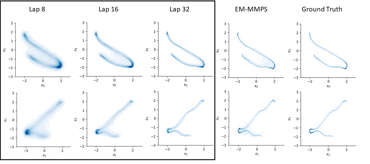
Figure 2: Evolution of the learned latent distribution on the synthetic manifold task. From left to right: reconstructed distributions from our model at DiffEM iterations 8, 16, and 32, followed by the distribution from EM-MMPS ([Rozet et al., 2024], 32th iteration) and the ground-truth $P_{X}^{\star}$. Our method shows progressively better concentration around the ground-truth curve, demonstrating more accurate posterior learning compared to previous work.

B.2 More details on the experiment in Section˜B.1

We implement the denoiser network $d_{\theta}(x,t|y)$ using a Multi-Layer Perceptron (MLP). The network architecture and training hyperparameters are detailed in Table 4.

Architecture	MLP
Input Shape	$5+2+5\times 2=17$
Hidden Layers	3
Hidden Layer Sizes	256, 256, 256
Activation	SiLU
Normalization	LayerNorm
Optimizer	Adam
Weight Decay	0
Scheduler	linear
Initial Learning Rate	$1\times 10^{-3}$
Final Learning Rate	$1\times 10^{-6}$
Gradient Norm Clipping	1.0
Batch Size	1024
Epochs in each iteration	65536
Sampler	Predictor-Corrector
Sampler Steps	4096
Number of EM iterations	32

Table 4: Network architecture and training hyperparameters for the MLP used in the synthetic manifold experiment.

To quantify the quality of the learned distribution, we compute the Sinkhorn divergence $S_{\lambda}$ Ramdas et al. [2015] with regularization parameter $\lambda=10^{-3}$ after each epoch. The Sinkhorn divergence is defined as:

$$S_{\lambda}(\mu,\nu) :=T_{\lambda}(\mu,\nu)-\frac{1}{2}(T_{\lambda}(\mu,\mu)+T_{\lambda}(\nu,\nu))$$

$$T_{\lambda}(\mu,\nu) :=\min_{\gamma\in\Pi(\mu,\nu)}\int_{(\mathbb{R}^{d})^{2}}\|y-x\|_{2}^{2}d\gamma(x,y)+2\lambda H(\gamma,\mu\otimes\nu)$$

We plot the evolution of Sinkhorn divergence over the iterations of DiffEM and EM-MMPS [Rozet et al., 2024] in Fig.˜3. We also plot the 2D marginals of the distributions reconstructed by DiffEM and EM-MMPS in Fig.˜4.

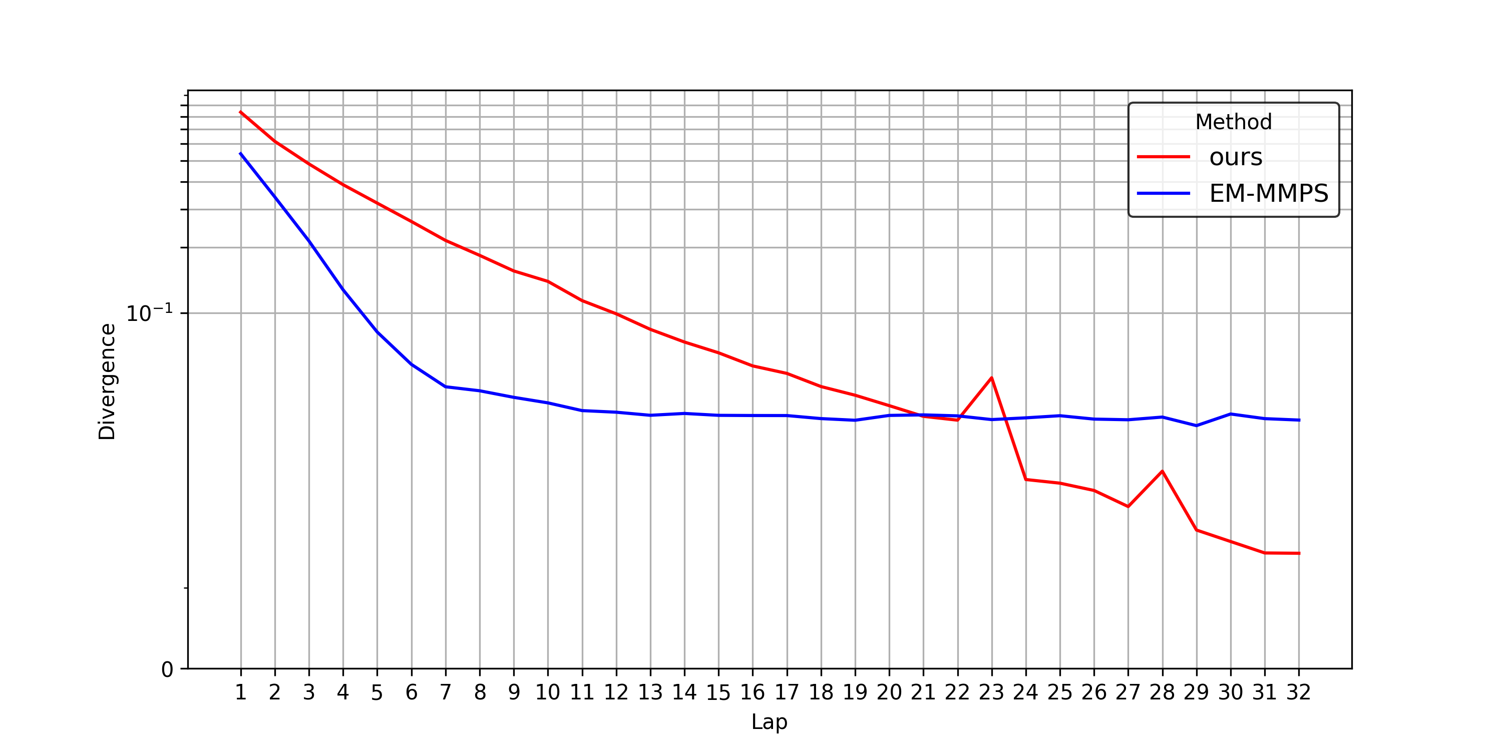
Figure 3: Evolution of Sinkhorn divergence between the ground-truth and reconstructed distributions during training. The red line shows DiffEM, and the blue line shows EM-MMPS.

Figure 3 demonstrates that while EM-MMPS provides effective initialization when the learned distribution is far from the true prior, it plateaus quickly and fails to achieve further improvements. This is likely due to the inherent approximation error of the approximate posterior sampling scheme (MMPS). In contrast, DiffEM continues to refine the reconstructed distribution, achieving better concentration around the ground-truth curve.

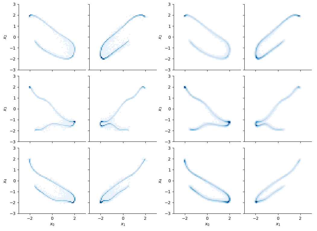
Figure 4: Comparison of 2D marginals of reconstructed distributions after the final iteration. Left: EM-MMPS; Right: DiffEM. DiffEM achieves better concentration around the ground-truth curve, indicating more accurate posterior learning.

B.3 Details of Masked CIFAR-10 (Section˜4.1)

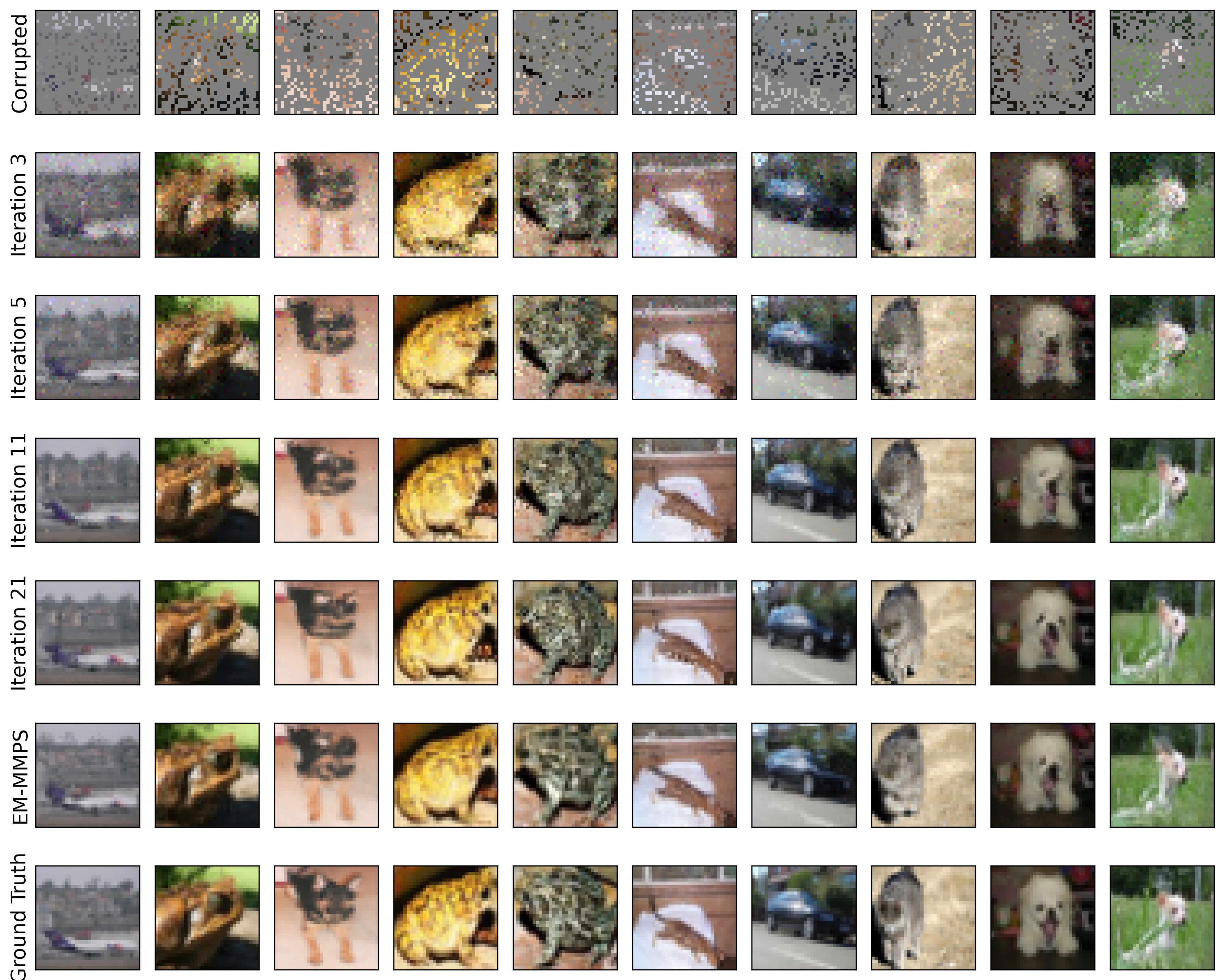
Figure 5: Qualitative comparison of reconstruction results on masked CIFAR-10 images. Top to bottom: corrupted input, EM-MMPS reconstructions, DiffEM reconstructions, and ground truth.

In this experiment, the conditional denoiser network $d_{\theta}$ is a U-Net Ronneberger et al. [2015], and we adopt the same experimental setup as Rozet et al. [2024] for a fair comparison. The only major difference in the architecture arises from the fact that our model is conditional and thus for the input we need to feed two images $X_{t}$ with shape $(32,32,3)$ and $Y$ with shape $(32,32,3)$ to the model, we concatenate the images on the third dimension and thus the input shape for the model is $(32,32,6)$, the output is also $(32,32,6)$ but in the whole training process we ignore the last three channels of the output. The details of network architecture and hyperparameters are presented in Table˜5.

Experiment	CIFAR-10	CelebA
Architecture	U-Net	U-Net
Input Shape	(32, 32, 6)	(64, 64, 6)
Channels Per Level	(128, 256, 384)	(128, 256, 384, 512)
Attention Heads per level	(0, 4, 0)	(0, 0, 0, 4)
Hidden Blocks	(5, 5, 5)	(3, 3, 3, 3)
Kernel Shape	(3, 3)	(3, 3)
Embedded Features	256	256
Activation	SiLU	SiLU
Normalization	LayerNorm	LayerNorm
Optimizer	Adam	Adam
Initial Learning Rate	$2\times 10^{-4}$	$1\times 10^{-4}$
Final Leanring Rate	$1\times 10^{-6}$	$1\times 10^{-6}$
Weight Decay	0	0
EMA	0.9999	0.999
Dropout	0.1	0.1
Gradient Norm Clipping	1.0	1.0
Batch Size	256	256
Epochs per EM iteration	256	64
Sampler	DDPM	DDPM

Table 5: Network architecture and training hyperparameters for the U-Net models used in the CIFAR-10 and CelebA experiments. Input shape varies by task.

We apply DiffEM with $K=21$ iterations to train our conditional diffusion model and evaluate its performance for the posterior sampling task as described in Section˜4.1. To evaluate the quality of the reconstructed prior, we also train an unconditional diffusion model with the same architecture on the reconstructed data. We compute the Inception Score (IS) Salimans et al. [2016] and the Fréchet Inception Distance (FID) Heusel et al. [2017] using the torch-fidelity package [Obukhov et al., 2021], and FD_DINOv2 [Oquab et al., 2023, Stein et al., 2023] and FD_∞ [Chong and Forsyth, 2020] using the codebase from [Stein et al., 2023]. The results are presented in Table˜1. We also note that the results of EM-MMPS are obtained with 32 iterations, following the original setup of Rozet et al. [2024].

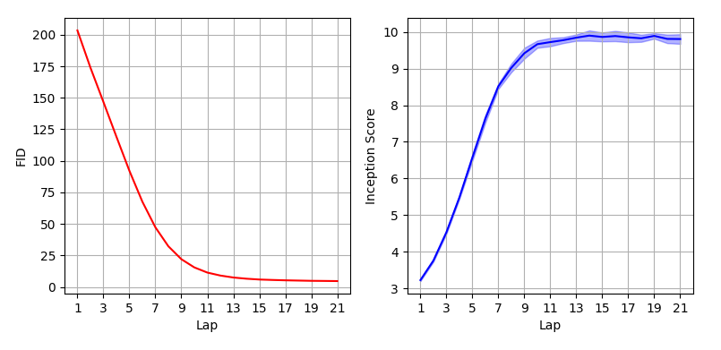
Figure 6: Evolution of evaluation metrics for posterior sampling measured during DiffEM training on CIFAR-10 with random masking. Left: FID, Right: Inception Score.

As an illustration, we also plot the evolution of the IS and FID during DiffEM iterations, demonstrating that DiffEM monotonically improves the quality of the reconstructed prior, in accordance with our theoretical results (Lemma˜1).

Experiments with higher corruption

In addition, we perform experiments on CIFAR-10 with corruption probability $\rho=0.9$ (i.e., $90\%$ of the pixels are randomly deleted) and present the results in Table˜6. Under such high corruptions, DiffEM also consistently outperforms EM-MMPS [Rozet et al., 2024].

Task	Method	IS $\uparrow$	FID $\downarrow$	FDDINOv2 $\downarrow$	FD∞ $\downarrow$
Posterior sampling	EM-MMPS	5.06	67.97	1045.51	1039.82
	DiffEM	5.86	46.13	915.69	912.26
Prior reconstruction	EM-MMPS	4.86	73.34	1174.13	1168.66
	DiffEM	5.46	49.10	1111.16	1107.64

Table 6: Performance of DiffEM and EM-MMPS on CIFAR-10 with $90\%$ random masking.

B.4 DiffEM with warm-start

We plot the evolution of IS, FID, FD_DINOv2 and FD_∞ scores during training in Fig.˜7.

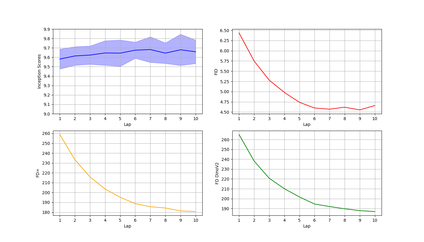
Figure 7: Evolution of IS, FID, DINO, FD_∞ during the 10 DiffEM iterations with the warm-started prior.

B.5 Details of Blurred CIFAR-10

In the experiment on CIFAR-10 with Gaussian blur, we set $\sigma_{\rm kernel}=2$ and $\sigma_{Y}^{2}=10^{-6}$. We apply DiffEM for $K=21$ iterations, with the same initialization, denoiser network architecture, and hyperparameters as in the masked CIFAR-10 experiment (detailed in Table˜5, Section˜B.3). Due to time constraints, we do not evaluate EM-MMPS [Rozet et al., 2024], as the moment-matching steps (based on the conjugate gradient method) are very time-consuming in this setting.

Qualitative study

To evaluate the quality of the trained conditional model, we sample a set of blurred images from the CIFAR-10 training set and use the trained model to generate a reconstruction for each image. We present the images in Fig.˜8.

Quantitative comparison

For comparison, we use the Richardson-Lucy deblurring algorithm Richardson [1972] as a baseline, which is a widely used method for image deconvolution. We also plot the evolution of the IS and FID during DiffEM iterations in Fig.˜9.

Method	IS $\uparrow$	FID $\downarrow$	FDDINOv2 $\downarrow$	FD∞ $\downarrow$
Richardson-Lucy deconvolution	3.72	131.74	1479.79	1470.78
DiffEM (Ours)	6.12	43.65	404.05	400.65

Table 7: Posterior sampling performance on CIFAR-10 with Gaussian blur ($\sigma_{\rm kernel}=2$).

Method	IS $\uparrow$	FID $\downarrow$	FDDINOv2 $\downarrow$	FD∞ $\downarrow$
DiffEM (Ours)	11.27	51.25	772.23	768.19

Table 8: Prior reconstruction performance on CIFAR-10 with Gaussian blur ($\sigma_{\rm kernel}=2$).

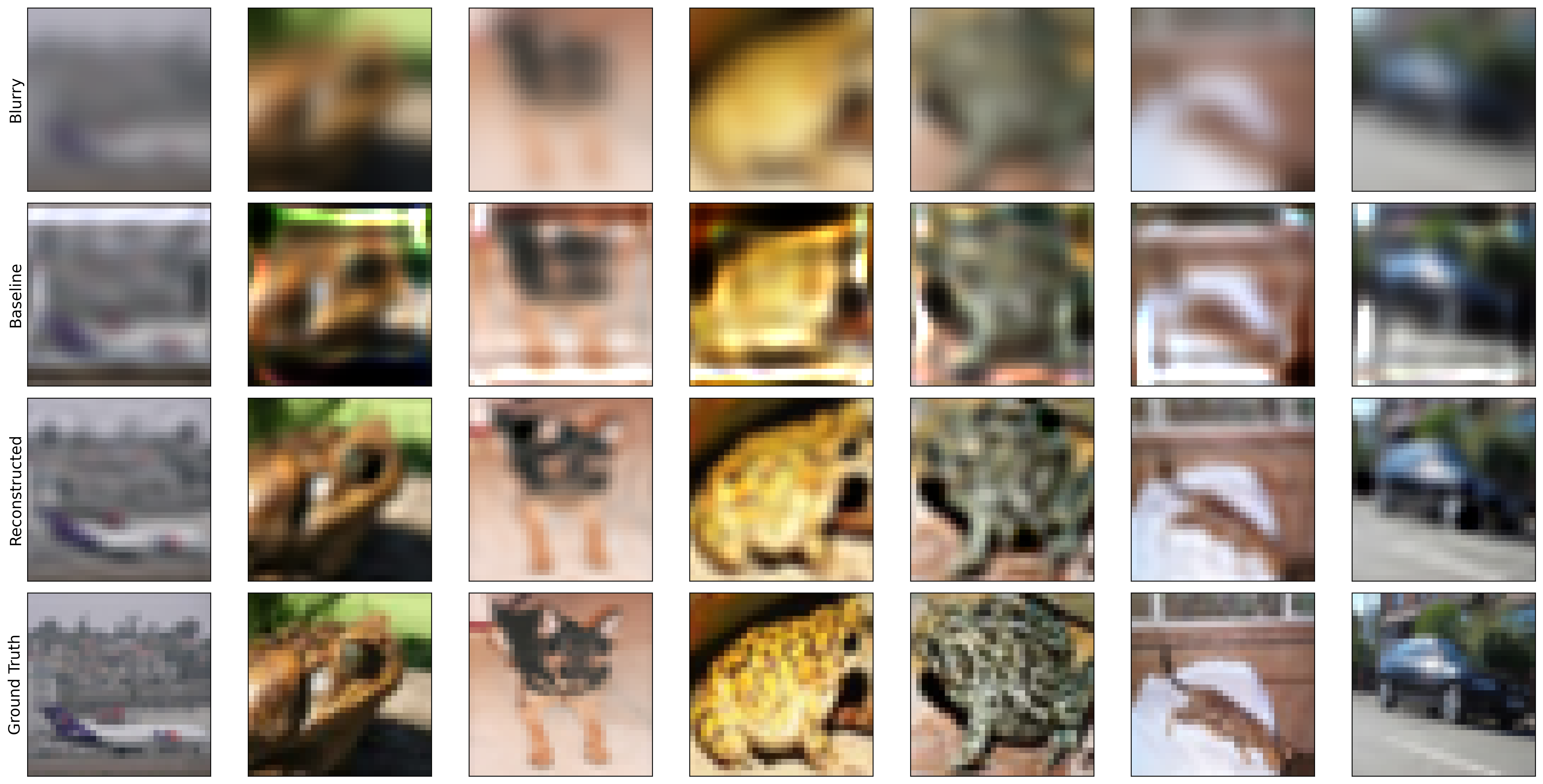
Figure 8: Qualitative results of image reconstruction from Gaussian blur. Top to bottom: blurred image, reconstruction by Richardson-Lucy deconvolution, image reconstructed by DiffEM model, and ground truth. DiffEM effectively recovers image details.

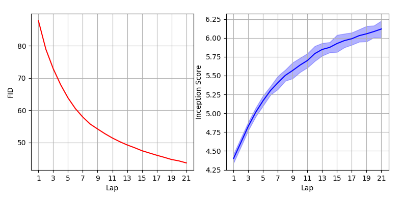
Figure 9: Evolution of evaluation metrics for posterior sampling measured during DiffEM training on CIFAR-10 with Gaussian blur. Left: FID, Right: Inception Score.

B.6 Masked CelebA

As a demonstration, we sample seven masked images from the CelebA training set under the $75\%$ corruption setting. Using the trained model, we generate reconstructions for each image after the $1^{\text{st}}$, $2^{\text{nd}}$, $4^{\text{th}}$, $8^{\text{th}}$, and $16^{\text{th}}$ iterations. The results are shown in Fig.˜10.

The denoiser architecture is detailed in Table˜5. For the $50\%$ corruption setting, we trained the conditional diffusion model for 20 EM iterations, while for the $75\%$ corruption setting we trained it for 24 iterations. In both cases, we trained EM-MMPS for 9 iterations. The computational overhead of Moment Matching Posterior Sampling becomes particularly evident in this experiment, as the CelebA dataset is larger (202,599 images) and each image is higher-dimensional ($64\times 64$) compared to CIFAR-10. We observed that each EM iteration of EM-MMPS required $4.85\pm 0.02$ hours, whereas each iteration of DiffEM required $1.19\pm 0.03$ hours.

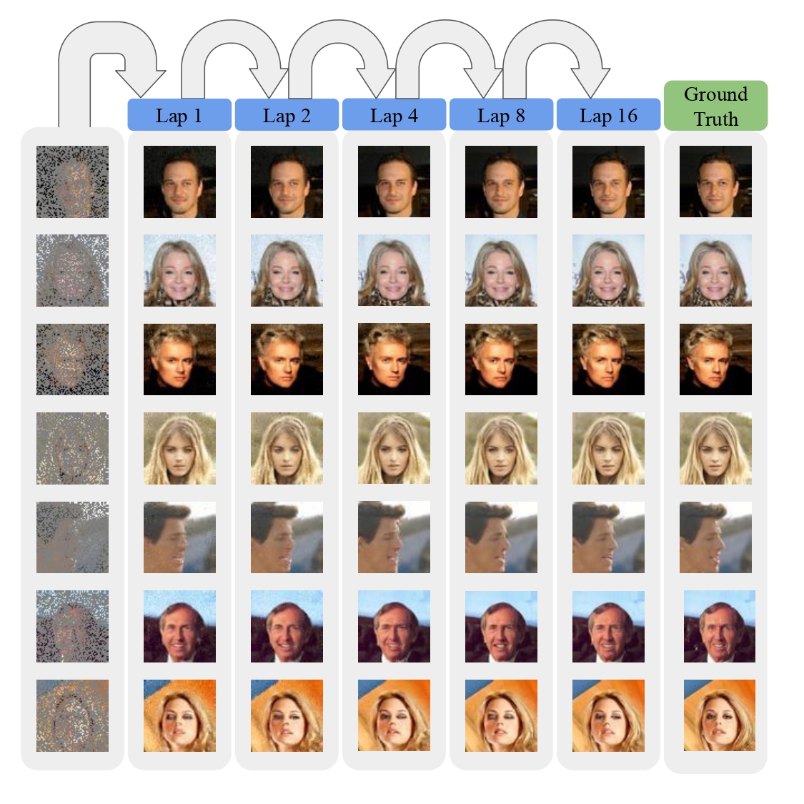
Figure 10: Qualitative results on the CelebA experiment under the $75\%$ corruption setting. The leftmost column shows samples from the dataset. The subsequent columns display reconstructions generated by the conditional diffusion model after laps $k=1,2,4,8,16$. The rightmost column shows the ground-truth images.

References

- Aali et al. [2023] Asad Aali, Marius Arvinte, Sidharth Kumar, and Jonathan I Tamir. Solving inverse problems with score-based generative priors learned from noisy data. arXiv preprint arXiv:2305.01166, 2023.
- Aali et al. [2025] Asad Aali, Giannis Daras, Brett Levac, Sidharth Kumar, Alex Dimakis, and Jon Tamir. Ambient diffusion posterior sampling: Solving inverse problems with diffusion models trained on corrupted data. In The Thirteenth International Conference on Learning Representations, 2025. URL https://openreview.net/forum?id=qeXcMutEZY.
- Aubin-Frankowski et al. [2022] Pierre-Cyril Aubin-Frankowski, Anna Korba, and Flavien Léger. Mirror descent with relative smoothness in measure spaces, with application to sinkhorn and em. Advances in Neural Information Processing Systems, 35:17263–17275, 2022.
- Bai et al. [2024] Weimin Bai, Yifei Wang, Wenzheng Chen, and He Sun. An expectation-maximization algorithm for training clean diffusion models from corrupted observations. arXiv preprint arXiv:2407.01014, 2024.
- Carlini et al. [2023] Nicolas Carlini, Jamie Hayes, Milad Nasr, Matthew Jagielski, Vikash Sehwag, Florian Tramer, Borja Balle, Daphne Ippolito, and Eric Wallace. Extracting training data from diffusion models. In 32nd USENIX Security Symposium (USENIX Security 23), pages 5253–5270, 2023.
- Chen et al. [2022] Sitan Chen, Sinho Chewi, Jerry Li, Yuanzhi Li, Adil Salim, and Anru R Zhang. Sampling is as easy as learning the score: theory for diffusion models with minimal data assumptions. arXiv preprint arXiv:2209.11215, 2022.
- Chen et al. [2024] Sitan Chen, Vasilis Kontonis, and Kulin Shah. Learning general gaussian mixtures with efficient score matching. arXiv preprint arXiv:2404.18893, 2024.
- Choi et al. [2021] Jooyoung Choi, Sungwon Kim, Yonghyun Jeong, Youngjune Gwon, and Sungroh Yoon. Ilvr: Conditioning method for denoising diffusion probabilistic models. arXiv preprint arXiv:2108.02938, 2021.
- Chong and Forsyth [2020] Min Jin Chong and David Forsyth. Effectively unbiased fid and inception score and where to find them. In Proceedings of the IEEE/CVF conference on computer vision and pattern recognition, pages 6070–6079, 2020.
- Chung et al. [2022] Hyungjin Chung, Jeongsol Kim, Michael T Mccann, Marc L Klasky, and Jong Chul Ye. Diffusion posterior sampling for general noisy inverse problems. arXiv preprint arXiv:2209.14687, 2022.
- Conforti et al. [2023] Giovanni Conforti, Alain Durmus, and Marta Gentiloni Silveri. Score diffusion models without early stopping: finite fisher information is all you need. arXiv e-prints, pages arXiv–2308, 2023.
- Conforti et al. [2025] Giovanni Conforti, Alain Durmus, and Marta Gentiloni Silveri. Kl convergence guarantees for score diffusion models under minimal data assumptions. SIAM Journal on Mathematics of Data Science, 7(1):86–109, 2025.
- Daras et al. [2023a] Giannis Daras, Yuval Dagan, Alexandros G Dimakis, and Constantinos Daskalakis. Consistent diffusion models: Mitigating sampling drift by learning to be consistent. arXiv preprint arXiv:2302.09057, 2023a.
- Daras et al. [2023b] Giannis Daras, Kulin Shah, Yuval Dagan, Aravind Gollakota, Alex Dimakis, and Adam Klivans. Ambient diffusion: Learning clean distributions from corrupted data. In Thirty-seventh Conference on Neural Information Processing Systems, 2023b. URL https://openreview.net/forum?id=wBJBLy9kBY.
- Daras et al. [2024a] Giannis Daras, Hyungjin Chung, Chieh-Hsin Lai, Yuki Mitsufuji, Jong Chul Ye, Peyman Milanfar, Alexandros G Dimakis, and Mauricio Delbracio. A survey on diffusion models for inverse problems. arXiv preprint arXiv:2410.00083, 2024a.
- Daras et al. [2024b] Giannis Daras, Alexandros G Dimakis, and Constantinos Daskalakis. Consistent diffusion meets tweedie: Training exact ambient diffusion models with noisy data. arXiv preprint arXiv:2404.10177, 2024b.
- Daras et al. [2025] Giannis Daras, Yeshwanth Cherapanamjeri, and Constantinos Costis Daskalakis. How much is a noisy image worth? data scaling laws for ambient diffusion. In The Thirteenth International Conference on Learning Representations, 2025. URL https://openreview.net/forum?id=qZwtPEw2qN.
- Dou et al. [2024] Zehao Dou, Subhodh Kotekal, Zhehao Xu, and Harrison H Zhou. From optimal score matching to optimal sampling. arXiv preprint arXiv:2409.07032, 2024.
- Gatmiry et al. [2024] Khashayar Gatmiry, Jonathan Kelner, and Holden Lee. Learning mixtures of gaussians using diffusion models. arXiv preprint arXiv:2404.18869, 2024.
- Heusel et al. [2017] Martin Heusel, Hubert Ramsauer, Thomas Unterthiner, Bernhard Nessler, and Sepp Hochreiter. Gans trained by a two time-scale update rule converge to a local nash equilibrium. In I. Guyon, U. Von Luxburg, S. Bengio, H. Wallach, R. Fergus, S. Vishwanathan, and R. Garnett, editors, Advances in Neural Information Processing Systems, volume 30. Curran Associates, Inc., 2017. URL https://proceedings.neurips.cc/paper_files/paper/2017/file/8a1d694707eb0fefe65871369074926d-Paper.pdf.
- Ho et al. [2020] Jonathan Ho, Ajay Jain, and Pieter Abbeel. Denoising diffusion probabilistic models. Advances in neural information processing systems, 33:6840–6851, 2020.
- Kawar et al. [2021] Bahjat Kawar, Gregory Vaksman, and Michael Elad. Snips: Solving noisy inverse problems stochastically. Advances in Neural Information Processing Systems, 34:21757–21769, 2021.
- Kawar et al. [2022] Bahjat Kawar, Michael Elad, Stefano Ermon, and Jiaming Song. Denoising diffusion restoration models. Advances in Neural Information Processing Systems, 35:23593–23606, 2022.
- Kawar et al. [2023] Bahjat Kawar, Noam Elata, Tomer Michaeli, and Michael Elad. Gsure-based diffusion model training with corrupted data. arXiv preprint arXiv:2305.13128, 2023.
- Krizhevsky [2009] Alex Krizhevsky. Learning multiple layers of features from tiny images. 2009. URL https://api.semanticscholar.org/CorpusID:18268744.
- Liu et al. [2018] Ziwei Liu, Ping Luo, Xiaogang Wang, and Xiaoou Tang. Large-scale celebfaces attributes (celeba) dataset. Retrieved August, 15(2018):11, 2018.
- Lu et al. [2025] Haoye Lu, Qifan Wu, and Yaoliang Yu. SFBD: A method for training diffusion models with noisy data. In Frontiers in Probabilistic Inference: Learning meets Sampling, 2025. URL https://openreview.net/forum?id=6HN14zuHRb.
- Obukhov et al. [2021] Anton Obukhov, Maximilian Seitzer, Po-Wei Wu, Semen Zhydenko, Jonathan Kyl, and Elvis Yu-Jing Lin. High-fidelity performance metrics for generative models in pytorch, 2020. Version: 0.3. 0, DOI, 10, 2021.
- Oquab et al. [2023] Maxime Oquab, Timothée Darcet, Théo Moutakanni, Huy Vo, Marc Szafraniec, Vasil Khalidov, Pierre Fernandez, Daniel Haziza, Francisco Massa, Alaaeldin El-Nouby, et al. Dinov2: Learning robust visual features without supervision. arXiv preprint arXiv:2304.07193, 2023.
- Ramdas et al. [2015] Aaditya Ramdas, Nicolas Garcia, and Marco Cuturi. On wasserstein two sample testing and related families of nonparametric tests, 2015. URL https://arxiv.org/abs/1509.02237.
- Richardson [1972] William Hadley Richardson. Bayesian-based iterative method of image restoration. J. Opt. Soc. Am., 62(1):55–59, Jan 1972. doi: 10.1364/JOSA.62.000055. URL https://opg.optica.org/abstract.cfm?URI=josa-62-1-55.
- Ronneberger et al. [2015] Olaf Ronneberger, Philipp Fischer, and Thomas Brox. U-net: Convolutional networks for biomedical image segmentation. In Nassir Navab, Joachim Hornegger, William M. Wells, and Alejandro F. Frangi, editors, Medical Image Computing and Computer-Assisted Intervention – MICCAI 2015, pages 234–241, Cham, 2015. Springer International Publishing. ISBN 978-3-319-24574-4.
- Rozet et al. [2024] François Rozet, Gérôme Andry, François Lanusse, and Gilles Louppe. Learning diffusion priors from observations by expectation maximization. arXiv preprint arXiv:2405.13712, 2024.
- Saharia et al. [2022] Chitwan Saharia, William Chan, Huiwen Chang, Chris Lee, Jonathan Ho, Tim Salimans, David Fleet, and Mohammad Norouzi. Palette: Image-to-image diffusion models. In ACM SIGGRAPH 2022 conference proceedings, pages 1–10, 2022.
- Salimans et al. [2016] Tim Salimans, Ian Goodfellow, Wojciech Zaremba, Vicki Cheung, Alec Radford, and Xi Chen. Improved techniques for training gans, 2016. URL https://arxiv.org/abs/1606.03498.
- Shah et al. [2025] Kulin Shah, Alkis Kalavasis, Adam R. Klivans, and Giannis Daras. Does generation require memorization? creative diffusion models using ambient diffusion, 2025.
- Somepalli et al. [2023a] Gowthami Somepalli, Vasu Singla, Micah Goldblum, Jonas Geiping, and Tom Goldstein. Diffusion art or digital forgery? investigating data replication in diffusion models. In Proceedings of the IEEE/CVF conference on computer vision and pattern recognition, pages 6048–6058, 2023a.
- Somepalli et al. [2023b] Gowthami Somepalli, Vasu Singla, Micah Goldblum, Jonas Geiping, and Tom Goldstein. Understanding and mitigating copying in diffusion models. arXiv preprint arXiv:2305.20086, 2023b.
- Song and Ermon [2019] Yang Song and Stefano Ermon. Generative modeling by estimating gradients of the data distribution. Advances in neural information processing systems, 32, 2019.
- Song et al. [2020] Yang Song, Jascha Sohl-Dickstein, Diederik P Kingma, Abhishek Kumar, Stefano Ermon, and Ben Poole. Score-based generative modeling through stochastic differential equations. arXiv preprint arXiv:2011.13456, 2020.
- Stein et al. [2023] George Stein, Jesse Cresswell, Rasa Hosseinzadeh, Yi Sui, Brendan Ross, Valentin Villecroze, Zhaoyan Liu, Anthony L Caterini, Eric Taylor, and Gabriel Loaiza-Ganem. Exposing flaws of generative model evaluation metrics and their unfair treatment of diffusion models. Advances in Neural Information Processing Systems, 36:3732–3784, 2023.
- Wang et al. [2016] Shanshan Wang, Zhenghang Su, Leslie Ying, Xi Peng, Shun Zhu, Feng Liang, Dagan Feng, and Dong Liang. Accelerating magnetic resonance imaging via deep learning. In International Symposium on Biomedical Imaging, 2016. doi: 10.1109/ISBI.2016.7493320.
- Wang et al. [2023] Zhendong Wang, Yifan Jiang, Huangjie Zheng, Peihao Wang, Pengcheng He, Zhangyang Wang, Weizhu Chen, and Mingyuan Zhou. Patch diffusion: Faster and more data-efficient training of diffusion models. arXiv preprint arXiv:2304.12526, 2023.
- Wibisono et al. [2024] Andre Wibisono, Yihong Wu, and Kaylee Yingxi Yang. Optimal score estimation via empirical bayes smoothing. In The Thirty Seventh Annual Conference on Learning Theory, pages 4958–4991. PMLR, 2024.
- Zbontar et al. [2018] Jure Zbontar, Florian Knoll, Anuroop Sriram, Tullie Murrell, Zhengnan Huang, Matthew J. Muckley, Aaron Defazio, Ruben Stern, Patricia Johnson, Mary Bruno, Marc Parente, Krzysztof J. Geras, Joe Katsnelson, Hersh Chandarana, Zizhao Zhang, Michal Drozdzal, Adriana Romero, Michael Rabbat, Pascal Vincent, Nafissa Yakubova, James Pinkerton, Duo Wang, Erich Owens, C. Lawrence Zitnick, Michael P. Recht, Daniel K. Sodickson, and Yvonne W. Lui. fastMRI: An Open Dataset and Benchmarks for Accelerated MRI. 2018. URL http://arxiv.org/abs/1811.08839.
- Zhang et al. [2024] Kaihong Zhang, Caitlyn H Yin, Feng Liang, and Jingbo Liu. Minimax optimality of score-based diffusion models: Beyond the density lower bound assumptions. arXiv preprint arXiv:2402.15602, 2024.