The $\alpha$–regression for compositional data: a unified framework for standard, spatially-lagged, and geographically-weighted regression models

Abstract

Compositional data—vectors of non-negative components summing to unity—frequently arise in scientific applications where covariates influence the relative proportions of components, yet traditional regression approaches struggle with the unit-sum constraint and zero values. This paper revisits the $\alpha$–regression framework, which uses a flexible power transformation parameterized by $\alpha$ to interpolate between raw data analysis and log-ratio methods, naturally handling zeros without imputation while allowing data-driven transformation selection. We formulate $\alpha$–regression as a non-linear least squares problem, provide efficient estimation via the Levenberg-Marquardt algorithm with explicit gradient and Hessian derivations, establish asymptotic normality of the estimators, and derive marginal effects for interpretation. The framework is extended to spatial settings through two models: the $\alpha$–spatially lagged X regression model, which incorporates spatial spillover effects via spatially lagged covariates with decomposition into direct and indirect effects, and the geographically weighted $\alpha$–regression, which allows coefficients to vary spatially for capturing local relationships. Application to Greek agricultural land-use data demonstrates that spatial extensions substantially improve predictive performance.

keywords: compositional data, $\alpha$–transformation, spatial regression

1 Introduction

Compositional data are vectors of non-negative components summing to a constant, typically equal 1, for simplicity purposes. Their sample space is the standard simplex

$$\mathbb{S}^{D-1}=\left\{(y_{1},...,y_{D})\ \big|\ y_{i}\geq 0,\sum_{i=1}^{D}y_{i}=1\right\},$$ (1)

where $D$ denotes the number of variables (better known as components).

Examples of compositional data may be found in many different fields of study and the extensive scientific literature that has been published on the proper analysis of this type of data is indicative of its prevalence in real-life applications.

It is unsurprising, given how frequently such data occur, that many applications of compositional data analysis incorporate explanatory variables. Examples include glacial compositional data, household consumption expenditures, concentrations of chemical elements in soil samples, morphometric fish measurements, as well as data on elections, pollution, and energy, all of which are associated with explanatory variables. Beyond these cases, the literature provides numerous further applications of compositional regression. For example, oceanography research involving Foraminiferal compositions at various sea depths was analyzed in Aitchison, (2003). In hydrochemistry, regression methods were used by Otero et al., (2005) to distinguish anthropogenic from geological sources of river pollution in Spain. Economic studies such as Morais et al., (2018) connected market shares with explanatory variables, while political science research linked candidate vote percentages to relevant predictors (Katz and King,, 1999). In bioinformatics, compositional approaches have also been applied to microbiome data analysis (Xia et al.,, 2013, Chen and Li,, 2016, Shi et al.,, 2016).

The practical demand for robust regression models tailored to compositional data has led to numerous methodological advances, especially in recent years. The first such model was introduced by Aitchison, (2003)—commonly known as Aitchison’s model—based on log-ratio transformations, yielding the log-ratio approach (LRA). Egozcue et al., (2003) advanced Aitchison’s model by applying an isometric log-ratio transformation. The stay-in-the-simplex approach on the other hand employs distributions and models defined on the simplex. Dirichlet regression for instance has been employed in compositional contexts Gueorguieva et al., (2008), Hijazi and Jernigan, (2009), Melo et al., (2009). Moreover, Iyengar and Dey, (2002) examined the generalized Liouville distribution family, which allows negative or mixed correlations and extends beyond Dirichlet distributions to include non-positive correlation structures. A not so popular approach is to ignore the compositional constraint and treat the data as though they were Euclidean, an approach termed raw data analysis (RDA) (Baxter,, 2001, Baxter et al.,, 2005). A fourth approach is to employ a general family of transformations, namely the $\alpha$–transformation (Tsagris et al.,, 2011) that interpolates between the and the RDA and the LRA, offers a higher flexibility and treats zero values naturally.

A limitation of the regression models discussed above is their inability to directly accommodate zero values. As a result, several models have been developed more recently to tackle this issue. For instance, Scealy and Welsh, (2011) mapped compositional data onto the unit hyper-sphere and proposed the Kent regression, which naturally accounts for zeros. From a Bayesian perspective, spatial compositional data containing zeros were modeled in Leininger et al., (2013). In the context of economics, Mullahy, (2015) estimated regression models for share data where the proportions could assume zero values with non-negligible probability. Further econometric approaches suitable for handling zeros are reviewed in Murteira and Ramalho, (2016). In addition, Tsagris, 2015a introduced a regression framework based on minimizing the Jensen–Shannon divergence. Tsagris and Stewart, (2018) extended Dirichlet regression to allow zeros, resulting in what is termed zero-adjusted Dirichlet regression. More recently, Alenazi, (2022) studied and examined the properties of the $\phi$-divergence regression models, which are suitable for compositional data with zeros.

When it comes spatial autocorrelation models, a simple version is the spatial distributed lag model with spatial lags on explanatory variables, commonly known as the spatially lagged X (SLX) model. Unlike the general spatial Durbin or spatial autoregressive models, the SLX model incorporates spatial dependence only through the explanatory variables, excluding the spatial lag of the dependent variable (LeSage and Pace,, 2009, Elhorst,, 2014).

A local form of linear regression, used to model spatially varying relationships, is the geographically weighted regression (GWR) is. Unlike traditional regression which assumes stationarity in the relationship between dependent and independent variables, GWR allows model parameters to vary over space. The integration of GWR with compositional data analysis is relatively recent. One key challenge is reconciling the spatial non-stationarity modeled by GWR with the constraints inherent in compositional data. Several approaches have been proposed. Leininger et al., (2013) combined GWR with hierarchical Bayesian frameworks for compositional data with zero values, allowing for spatial priors that account for local variation. Yoshida et al., (2021) applied the isometric log-ratio (ilr) transformation before applying GWR. This preserves the relative information between parts while enabling spatially varying coefficient estimation. Finally, Clarotto et al., (2022) introduced a new power transformation, similar in spirit to the $\alpha$–transformation, for geostatistical modeling of compositional data.

The paper takes the pragmatic view, which seems especially relevant for regression problems (in which out-of-sample accurate predictions provide an objective measure of performance), that one should adopt whichever approach performs best in a given setting. The contribution of this paper is to revisit the $\alpha$–regression (Tsagris, 2015b, ), a generalization of Aitchison’s log-ratio regression that treats zero values naturally. The regression parameters of the $\alpha$–regression are estimated using a modification of the Levenberg-Marquardt algorithm and the relevant gradient vector, and the Hessian matrix are provided. Then, the $\alpha$–regression is extended to the $\alpha$–SLX model and is further extended to account for spatial weights, yielding the geographically weighted $\alpha$–regression (GW$\alpha$R).

The next section discusses the $\alpha$–regression, while section 3 extends this model to its GWR version. Section 4 illustrates the performance of the GW$\alpha$R on a real dataset and Section 5 concludes the paper.

2 The $\alpha$–regression

First the $\alpha$–transformation, used for the $\alpha$–regression, is defined, followed by the regression formulation.

2.1 The $\alpha$–transformation

Tsagris et al., (2011) introduced the $\alpha$–transformation, a power-based mapping designed for compositional data, $\bm{y}=(y_{1},y_{2},\ldots,y_{D})$. For a given parameter $\alpha\in[-1,1]$, the transformation is defined in two steps. Each component is raised to the power $\alpha$ and renormalized to remain in the simplex

$$\bm{u}=\left(\frac{y_{i}^{\alpha}}{\sum_{j=1}^{D}y_{j}^{\alpha}},\ldots,\frac{y_{D}^{\alpha}}{\sum_{j=1}^{D}y_{j}^{\alpha}}\right).$$ (2)

This ensures $u=(u_{1},\ldots,u_{D})$ is itself a composition. To map compositions into Euclidean space for analysis, apply a linear transformation using the $D\times(D-1)$ Helmert sub-matrix $\bm{H}$:

$$\bm{y}_{\alpha}=\frac{1}{\alpha}\left(D\bm{u}-1\right)\bm{H}^{\top},$$ (3)

where $1$ denotes the $D$-dimensional vector of ones.

The transformation in Equation (3) is a one-to-one transformation which maps data inside the simplex onto a subset of $\mathbb{R}^{d}$ and vice versa for $\alpha\neq 0$. The corresponding sample space of Equation (3) is

$$\mathbb{A}_{\alpha}^{d}=\left\{\bm{H}\bm{w}_{\alpha}(\bm{y})\ \big|-\frac{1}{\alpha}\leq w_{i,\alpha}\leq\frac{d}{\alpha},\sum_{i=1}^{d}w_{i,\alpha}=0\right\},$$ (4)

where $d=D-1$.

In effect, $y_{\alpha}$ which resembles a Box–Cox style mapping. The result $y_{\alpha}$ is an unconstrained vector in Euclidean space, suitable for standard multivariate statistical techniques. When $\alpha=1$, the transformation corresponds (up to scaling) to raw data analysis (RDA). When $\alpha=-1$, the transformation is aligned with RDA as well, but using the inverse of the compositional data. As $\alpha\to 0$, the transformation converges to the ilr transformation used in log-ratio analysis (LRA)

$$\bm{y}_{0}=\left(\log\left({\frac{y_{1}}{\prod_{j=1}^{D}x_{j}^{1/D}}}\right),\ldots,\log\left({\frac{y_{D}}{\prod_{j=1}^{D}y_{j}^{1/D}}}\right)\right)\bm{H}^{\top}.$$ (5)

Thus, the $\alpha$–transformation provides a continuum between RDA and LRA, allowing analysts to choose the most appropriate representation of compositional data based on empirical performance or theoretical considerations.

2.2 The $\alpha$–regression

The $\alpha$–regression has the potential to improve the regression predictions with compositional data by adapting the $\alpha$–transformation to the dataset’s geometry. We assume that the conditional mean of the observed composition can be written as a non-linear function of some explanatory variables

$$\mu_{i}=\begin{cases}\displaystyle\frac{1}{1+\sum_{j=1}^{D}e^{\mathbf{x}^{\top}\bm{\beta}_{j}}}&\text{for }i=1\\[12.91663pt] \displaystyle\frac{e^{\mathbf{x}^{\top}\bm{\beta}_{i}}}{1+\sum_{j=1}^{D}e^{\mathbf{x}^{\top}\bm{\beta}_{j}}}&\text{for }i=2,\ldots,D\end{cases}$$ (6)

where

$$\boldsymbol{\beta}_{i}=\left(\beta_{0i},\beta_{1i},...,\beta_{pi}\right)^{\top},\ i=1,...,d\ \ \text{and $p$ denotes the number of explanatory variables}.$$

Tsagris, 2015b used the log-likelihood of the multivariate normal distribution, but in this paper the regression is formulated as a non-linear least squares problem, where the minimizing function is

$$SSE\left(\bm{Y},\bm{X};\alpha,\bm{B}\right)=\sum_{i=1}^{n}\left(\bm{y}_{i,\alpha}-\bm{\mu}_{i,\alpha}\right)^{\top}\left(\bm{y}_{i,\alpha}-\bm{\mu}_{i,\alpha}\right)=tr\left[\left(\bm{y}_{\alpha}-\bm{\mu}_{\alpha}\right)\left(\bm{y}_{\alpha}-\bm{\mu}_{\alpha}\right)^{\top}\right],$$ (7)

where $\bm{y}_{i,\alpha}$ and $\bm{m}_{i,\alpha}$ are the $\alpha$–transformations applied to the $i$-th response and fitted compositional vectors, respectively. Note that when the stay-in-the-simplex power transformation (2) is applied to the fitted vectors, a simplification occurs

$$\frac{\mu_{i}^{\alpha}}{\sum_{j=1}^{D}\mu_{j}^{\alpha}}=\frac{\left(\frac{e^{{\bf x}^{\top}\boldsymbol{\beta}_{i}}}{1+\sum_{j=1}^{D}e^{{\bf x}^{\top}\boldsymbol{\beta}_{j}}}\right)^{\alpha}}{\frac{1+\sum_{k=1}^{D}\left(e^{{\bf x}^{\top}\boldsymbol{\beta}_{k}}\right)^{\alpha}}{\left(1+\sum_{j=1}^{D}e^{{\bf x}^{\top}\boldsymbol{\beta}_{j}}\right)^{\alpha}}}=\frac{\left(e^{{\bf x}^{\top}\boldsymbol{\beta}_{i}}\right)^{\alpha}}{1+\sum_{j=1}^{D}\left(e^{{\bf x}^{\top}\boldsymbol{\beta}_{i}}\right)^{\alpha}}.$$

For a given value of $\alpha$, the matrix of the regression coefficients $\bm{B}=\left(\bm{\beta}_{1},\ldots,\bm{\beta}_{d}\right)$ is estimated using a modification of the Levenberg-Marquardt algorithm. The R package minpack.lm (Elzhov et al.,, 2023) is employed to this end.

2.2.1 Limiting case of $\alpha\rightarrow 0$

Tsagris et al., (2016) presented the proof that as $\alpha\rightarrow 0$, the $\alpha$–transformation (3) converges to the ilr transformation (5). Following similar calculations one can show that

$$\lim_{\alpha\rightarrow 0}{\frac{1}{\alpha}\left(D\frac{\mu_{i}^{\alpha}}{\sum_{j=1}^{D}\mu_{j}^{\alpha}}-1\right)}\rightarrow\bm{x}\beta_{i}-\frac{\sum_{j=1}^{D}\bm{x}\beta_{j}}{D},$$

which corresponds to the regression after the centered log-ratio transformation [the ilr transformation (5) without the right multiplication by the Helmert matrix]. This implies that there are $D$ vectors of $\bm{\beta}$ regression coefficients. But, since the first set of regression coefficients equals zero, if we subtract this vector from the rest of the $\bm{\beta}$ vectors we end up with the regression coefficients of the additive log-ratio (alr) regression

$$\log\left(\frac{y_{i}}{y_{1}}\right)=\bm{x}^{\top}\boldsymbol{\beta}_{i},\ \ i=2,\ldots,D$$

2.2.2 Choosing $\alpha$

In the regression setting the optimal value of $\alpha$ is data-driven. The $\alpha$ is seen as hyper-parameter whose value is chosen by minimizing a divergence measure, such as the Kullback–Leibler divergence (KLD), between the observed and fitted compositions (Tsagris, 2015b, ).

2.2.3 Asymptotic properties of the regression coefficients

The following result extends the classic asymptotic theory of nonlinear least squares estimators (Jennrich,, 1969, Wu,, 1981, Amemiya,, 1985, Gallant,, 1987) to the multivariate regression setting.

Theorem 2.1 (Asymptotic normality of multivariate NLS estimators).

Let $\{(Y_{i},X_{i})\}_{i=1}^{n}$ be i.i.d. with $Y_{i}\in\mathbb{R}^{m}$ and $X_{i}\in\mathcal{X}$. Suppose

$$Y_{i}=g(X_{i},\beta_{0})+\varepsilon_{i},$$

where $g:\mathcal{X}\times\Theta\to\mathbb{R}^{m}$ is twice continuously differentiable in $\beta\in\Theta\subset\mathbb{R}^{p}$, $\beta_{0}$ is the true parameter, and $E[\varepsilon_{i}\mid X_{i}]=0$, $Var(\varepsilon_{i}\mid X_{i})=\Omega_{i}$. Define the Jacobian

$$G_{i}(\beta):=\frac{\partial}{\partial\beta^{\prime}}g(X_{i},\beta)\quad(m\times p).$$

Let $\hat{\beta}$ minimize the nonlinear least squares criterion

$$\hat{\beta}=\arg\min_{\beta\in\Theta}\;S_{n}(\beta),\qquad S_{n}(\beta)=\sum_{i=1}^{n}\|Y_{i}-g(X_{i},\beta)\|^{2}.$$

Assumptions:

• (Identifiability): $E[\|g(X_{i},\beta)-g(X_{i},\beta_{0})\|^{2}]=0\iff\beta=\beta_{0}$.

• (Interior point): $\beta_{0}$ lies in the interior of $\Theta$.

• (Smoothness): $g(x,\beta)$ is twice continuously differentiable in a neighborhood of $\beta_{0}$ for a.e. $x$.

• (Moment conditions): $E[\|\varepsilon_{i}\|^{2}]<\infty$ and conditions for a multivariate CLT and LLN hold.

• (Nonsingularity): The limit

  $$H=\mathop{\mathrm{plim}}_{n\to\infty}\frac{1}{n}\sum_{i=1}^{n}G_{i}(\beta_{0})^{\prime}G_{i}(\beta_{0})$$

  exists and is positive definite.

Under (A1)–(A5),

$$\sqrt{n}(\hat{\beta}-\beta_{0})\;\;\xrightarrow{d}\;\;N\!\left(0,\;H^{-1}JH^{-1}\right),$$

where

$$J=\mathop{\mathrm{plim}}_{n\to\infty}\frac{1}{n}\sum_{i=1}^{n}G_{i}(\beta_{0})^{\prime}\,\Omega_{i}\,G_{i}(\beta_{0}).$$

Special case: If $\varepsilon_{i}$ are i.i.d. with $Var(\varepsilon_{i})=\Sigma$, then

$$H=E\big[G_{i}(\beta_{0})^{\prime}G_{i}(\beta_{0})\big],\quad J=E\big[G_{i}(\beta_{0})^{\prime}\Sigma\,G_{i}(\beta_{0})\big].$$

If in addition $\Sigma=\sigma^{2}I_{m}$, then

$$\sqrt{n}(\hat{\beta}-\beta_{0})\;\;\xrightarrow{d}\;\;N\!\left(0,\;\sigma^{2}H^{-1}\right).$$

Sketch of proof.

The first-order condition is

$$0=-2\sum_{i=1}^{n}G_{i}(\hat{\beta})^{\prime}\big(Y_{i}-g(X_{i},\hat{\beta})\big).$$

Expanding around $\beta_{0}$ using $Y_{i}=g(X_{i},\beta_{0})+\varepsilon_{i}$ and a Taylor expansion of $g$ yields

$$\Bigg(\sum_{i=1}^{n}G_{i}(\beta_{0})^{\prime}G_{i}(\beta_{0})\Bigg)(\hat{\beta}-\beta_{0})=\sum_{i=1}^{n}G_{i}(\beta_{0})^{\prime}\varepsilon_{i}+o_{p}(\sqrt{n}).$$

Divide by $\sqrt{n}$ and apply a multivariate CLT to $n^{-1/2}\sum_{i}G_{i}(\beta_{0})^{\prime}\varepsilon_{i}\Rightarrow N(0,J)$. Since $n^{-1}\sum_{i}G_{i}(\beta_{0})^{\prime}G_{i}(\beta_{0})\to H$, Slutsky’s theorem gives the result. ∎

The asymptotic normality of the regression coefficients holds true as $\alpha\rightarrow 0$. We claim that it holds true for general values of $\alpha$, but since the space of the $\alpha$–transformation (4) is a subset of the Euclidean space, perhaps the proof requires more rigor and probably stricter assumptions.

Since the Hessian matrix is not exact, it is advised to use bootstrap to estimate

2.2.4 Marginal effects

To account for the difficult interpretation of the regression coefficients, the marginal effects are given below

$$\frac{\partial\mu_{i}}{\partial x_{k}}=\left\{\begin{array}[]{ll}-\mu_{1}\sum_{j=1}^{d}\beta_{jk}\mu_{j+1}&\text{for}\ \ i=1\\ \mu_{i}\left(\beta_{i-1,k}-\sum_{j=1}^{d}\beta_{jk}\mu_{j+1}\right)&\text{for}\ \ i=2,\ldots,D\end{array}\right\},$$ (10)

where $\sum_{i=1}^{D}\frac{\partial\mu_{i}}{\partial x_{k}}=0$. The sum of the marginal effects sums to zero, because if all components increase, one at least component must decrease by the same amount so that the unity sum constraint is preserved.

The average marginal effects (AME) across all observations are then computed as

$$\text{AME}_{k}=\frac{1}{n}\sum_{i=1}^{n}\frac{\partial\mu_{i}}{\partial x_{k}}$$

Standard errors can be computed via bootstrap or the delta method, accounting for estimation uncertainty in both $\hat{\bm{\beta}}$, $\hat{\bm{\gamma}}$, and $\hat{\bm{\mu}}$.

2.2.5 Advantages and Limitations

The advantages of the $\alpha$–regression are: a) ability to handle zeros naturally without imputation. b) Flexible, as $\alpha$ provides a continuum from power transforms to log-ratio methods. c) Often yields better predictive performance than classical methods. d) This method balances the strengths of power transformations and log-ratio methods, providing a flexible and effective tool for predictive modeling on the simplex. Disadvantages on the other hand are a) the interpretability of regression coefficients is reduced compared to log-ratio approaches. b) The focus is mainly on prediction rather than inference; theoretical properties of estimators have not been developed.

3 Spatial regression models

3.1 The SLX model

The SLX model provides a useful and interpretable framework for identifying spatial spillover effects through explanatory variables alone. While it lacks the feedback mechanisms of models that include $Wy$ (spatial autocorrelation of the dependent variable), it remains a robust and easily estimable tool for exploring spatial interactions. The structure of the SLX model allows researchers to capture how characteristics of neighboring spatial units affect local outcomes without introducing simultaneity. The general form of the SLX model is

$$y_{i}=\beta_{0}+\sum_{k=1}^{p}\beta_{k}x_{ik}+\sum_{k=1}^{p}\gamma_{k}\left(\sum_{j\neq i}w_{ij}x_{ik}\right)+\varepsilon_{i},$$ (11)

where $y$ denotes the dependent variable, $x_{k}$ denotes the $k$t-h explanatory variable, $w_{ij}$ is the $(i,j)$ element of the $n\times n$ spatial weights (contiguity) matrix $\bm{W}$ representing the spatial relationships between observations (e.g., contiguity or inverse distance), and $\sum_{j\neq i}w_{ij}x_{k}$ denotes the $k$-th spatially lagged explanatory variable. The $\beta s$ and $\gamma s$ are parameters corresponding to the direct (local) and indirect (spillover) effects, respectively, and $\varepsilon$ is the classical error term.

The inclusion of both $X$ and $WX$ enables the separation of effects into the Direct effects ($\beta s$): the impact of local explanatory variables on the local dependent variable. Indirect or spillover effects ($\gamma s$): the impact of explanatory variables from neighboring regions on the local dependent variable.

The classical form of the contiguity matrix contains elements $w_{ij}=1$ if areas $i$ and $j$ are neighbors and $0$ otherwise.

3.2 GWR model

GWR has become a widely used technique in spatial statistics for modeling spatially varying relationships. Traditional regression assumes stationarity of relationships across space, but GWR relaxes this assumption by allowing coefficients to vary geographically (Brunsdon et al.,, 1996). Meanwhile, compositional data–datasets where variables represent proportions of a whole and are constrained to sum to unity–have gained attention in many disciplines, including environmental sciences, geology, and social sciences. When spatial heterogeneity and compositional constraints intersect, specialized methodological developments are required. The foundational work of Fotheringham et al., (2002) formalized GWR as a local regression technique that incorporates spatial weighting functions to account for the geographical location of observations.

The basic form of a standard multiple linear regression is:

$$y_{i}=\beta_{0}+\sum_{k=1}^{p}\beta_{k}x_{ik}+\varepsilon_{i},$$

where $y$ denotes the dependent variable, $x_{k}$ is the $k$-th explanatory variable, the $\beta s$ are the regression parameters, and $\varepsilon_{i}$ is the error term, for $i=1,\ldots,n$.

In GWR, the parameters are allowed to vary with location:

$$y_{i}=\beta_{0}(\nu_{i},v_{i})+\sum_{k=1}^{p}\beta_{k}(\nu_{i},v_{i})\,x_{ik}+\varepsilon_{i},$$

where $(\nu_{i},v_{i})$ denotes the spatial coordinates of observation $i$ ($\nu_{i}$ and $v_{i}$ typically correspond to latitude and longitude, respectively), and $\beta_{k}(\nu_{i},v_{i})$ are the location-specific parameter estimates.

For each location $(u_{i},v_{i})$, the parameter vector is estimated as:

$$\hat{\bm{\beta}}(\nu_{i},v_{i})=\left(X^{\top}W(\nu_{i},v_{i})X\right)^{-1}X^{\top}W(\nu_{i},v_{i})\mathbf{y},$$

where $X$ is the design matrix and $W(\nu_{i},v_{i})$ is a spatial weighting matrix assigning higher weights to observations closer to $(\nu_{i},v_{i})$. A common weighting function is the Gaussian kernel

$$w_{ij}=\exp\left(-\frac{d_{ij}^{2}}{2h^{2}}\right),$$ (12)

where $d_{ij}$ is the distance between location $i$ and $j$, and $h$ is the bandwidth parameter controlling the degree of spatial smoothing.

4 The $\alpha$–SLX and GW$\alpha$R models

4.1 The $\alpha$–SLX model

The $\alpha$–SLX model extends the standard $\alpha$-regression by incorporating spatial spillover effects through the explanatory variables. The fitted compositional values are given by:

$$\mu_{i}=\begin{cases}\displaystyle\frac{1}{1+\sum_{j=1}^{D}e^{\mathbf{x}^{\top}\bm{\beta}_{j}+(\mathbf{W}\mathbf{x})^{\top}\bm{\gamma}_{j}}}&\text{for }i=1\\[12.91663pt] \displaystyle\frac{e^{\mathbf{x}^{\top}\bm{\beta}_{i}+(\mathbf{W}\mathbf{x})^{\top}\bm{\gamma}_{i}}}{1+\sum_{j=1}^{D}e^{\mathbf{x}^{\top}\bm{\beta}_{j}+(\mathbf{W}\mathbf{x})^{\top}\bm{\gamma}_{j}}}&\text{for }i=2,\ldots,D\end{cases}$$ (13)

The matrices of regression coefficients $\bm{B}=\left(\bm{\beta}_{1},\ldots,\bm{\beta}_{d}\right)$ and $\bm{\Gamma}=\left(\bm{\gamma}_{1},\ldots,\bm{\gamma}_{d}\right)$ in the same way as in the $\alpha$–regression.

4.1.1 The contiguity matrix

The Euclidean distance between any two pairs of latitude and longitude, $(\nu_{i},v_{i})$ and $(\nu_{j},v_{j})$. As mentioned earlier, the locations are first mapped from their polar to their Cartesian coordinates (after transforming the degrees into radians)

$$\bm{c}_{i}=\left(\cos(\nu_{i}),sin(\nu_{i})\cos(v_{i}),\sin(\nu_{i})\sin(v_{i})\right)\ \text{and}\ \bm{c}_{j}=\left(\cos(\nu_{j}),sin(\nu_{j})\cos(v_{j}),\sin(\nu_{j})\sin(v_{j})\right).$$

The Euclidean distance between $\bm{c}_{i}$ and $\bm{c}_{j}$ is

$$d(\bm{c}_{i},\bm{c}_{j})=d_{ij}^{2}=\left\|\bm{c}_{i}-\bm{c}_{j}\right\|^{2}=\left\|\bm{c}_{i}\right\|^{2}+\left\|\bm{c}_{j}\right\|^{2}-2\bm{c}_{i}^{\top}\bm{c}_{j}=2\left(1-\bm{c}_{i}^{\top}\bm{c}_{j}\right).$$

For the $i$-th location, compute the region with the the $k$ nearest neighbors $\mathcal{C}_{ik}$ and zero the rest, that is

$$\tilde{w}_{ij}=\begin{cases}1/d_{ij}^{2}&\text{if}\ j\in\mathcal{C}_{ik}\\ \tilde{w}_{ij}=0&\text{else}.\end{cases}$$ (14)

The $(i,j)$ elemets of the contiguity matrix $\bm{W}$ are then defined as $w_{ij}=\tilde{w}_{ij}/\sum_{j=1}^{n}\tilde{w}_{ij}$.

4.1.2 Choosing $\alpha$

The choice of the optimal values of $\alpha$ and of $k$ is again data-driven and can be performed via the leave one out cross validation (LOOCV) protocol, where the metric of performance is again the KLD.

4.1.3 Spatial marginal Effects

The direct marginal effects measure the impact of a change in the local explanatory variable $x_{k}$ on the local composition component $\mu_{i}$. The following formulas are identical to the standard $\alpha$–regression marginal effects (10), as they depend only on the $\bm{\beta}$ coefficients and do not involve spatial terms.

$$\frac{\partial\mu_{i}}{\partial x_{k}}=\begin{cases}-\mu_{1}\sum_{j=1}^{d}\beta_{jk}\mu_{j+1}&\text{for }i=1\\ \mu_{i}\left(\beta_{i-1,k}-\sum_{j=1}^{d}\beta_{jk}\mu_{j+1}\right)&\text{for }i=2,\ldots,D.\end{cases}$$ (15)

The indirect (spillover) marginal effects measure the impact of a change in the spatially lagged explanatory variable $(\mathbf{W}\mathbf{x})_{k}$ (i.e., the weighted average of neighboring values) on the local composition component $\mu_{i}$. They have the same functional form as the direct effects, with $\bm{\gamma}$ replacing $\bm{\beta}$. This structural symmetry reflects how spatial spillovers operate through the same multiplicative mechanism as direct effects.

$$\frac{\partial\mu_{i}}{\partial(\mathbf{W}\mathbf{x})_{k}}=\begin{cases}-\mu_{1}\sum_{j=1}^{d}\gamma_{jk}\mu_{j+1}&\text{for }i=1\\ \mu_{i}\left(\gamma_{i-1,k}-\sum_{j=1}^{d}\gamma_{jk}\mu_{j+1}\right)&\text{for }i=2,\ldots,D.\end{cases}$$ (16)

The total marginal effect combines both direct and indirect effects, representing the full impact of a simultaneous change in both local and neighboring explanatory variable values.

$$\frac{\partial\mu_{i}}{\partial x_{k}}+\frac{\partial\mu_{1}}{\partial(\mathbf{W}\mathbf{x})_{k}}=\begin{cases}-\mu_{1}\sum_{j=1}^{d}(\beta_{jk}+\gamma_{jk})\mu_{j+1}&\text{for }i=1\\ \mu_{i}\left[(\beta_{i-1,k}+\gamma_{i-1,k})-\sum_{j=1}^{d}(\beta_{jk}+\gamma_{jk})\mu_{j+1}\right]&\text{for }i=2,\ldots,D.\end{cases}$$ (17)

4.1.4 Properties of the spatial marginal effects

Some properties regarding the spatial marginal effects are delineated below.

• The sum of marginal effects across all components equals zero:

  $$\sum_{i=1}^{D}\frac{\partial\mu_{i}}{\partial x_{k}}=0\quad\text{and}\quad\sum_{i=1}^{D}\frac{\partial\mu_{i}}{\partial(\mathbf{W}\mathbf{x})_{k}}=0$$ (18)

  This ensures that the composition remains on the simplex after perturbations.

• All marginal effects depend on the current composition values $\bm{\mu}$, making them observation-specific and state-dependent.

• Direct and indirect effects share the same functional form, differing only in the coefficient vectors used ($\bm{\beta}$ vs. $\bm{\gamma}$).

• The spatial weights matrix $\mathbf{W}$ determines which neighbors contribute to spillover effects. Row-standardization is typically used such that $\sum_{j}w_{ij}=1$.

4.2 The GW$\alpha$R model

The GWR$\alpha$R model is a weighted $\alpha$–regression scheme, but the difference is that the regression is performed $n$ times, each time with different weights. The weighted $SSE$ that must be minimized is

$$SSE\left(\bm{Y},\bm{X};\alpha,h,\bm{B}\right)=\sum_{i=1}^{n}\left(\bm{y}_{i,\alpha}-\bm{\mu}_{i,\alpha}\right)^{\top}\bm{W}_{i}\left(\bm{y}_{i,\alpha}-\bm{\mu}_{i,\alpha}\right),$$ (19)

where $\bm{W}_{i}=\text{diag}\left\{w_{i1},\ldots,w_{in}\right\}$, is the weighting matrix corresponding to the weights allocated for the $i$-th observation.

As $\alpha\rightarrow 0$, the GW$\alpha$R converges to the GWR after the alr transformation (Yoshida et al.,, 2021).

4.2.1 Computing $d_{ij}$ in the weighting scheme

Some researchers tend to compute the Euclidean distance between two pairs of latitude and longitude, $(\nu_{i},v_{i})$ and $(\nu_{j},v_{j})$, $d_{ij}=\sqrt{\left(\nu_{i}-\nu_{j}\right)^{2}+\left(v_{i}-v_{j}\right)^{2}}$. There is a fundamental flaw with this approach which is highlighted by Mardia and Jupp,, 2000, pg. 13. Take for instance the case of two coordinates whose latitude (or longitude) values are $359^{\circ}$ and $1^{\circ}$. Using the previous naive approach yields a distance between the two values $359^{\circ}-1^{\circ}=358^{\circ}$, but the actual distance between them is only $2^{\circ}$. To account for this, the pair of coordinates must first be transformed into their Euclidean coordinates, prior to the application of the Euclidean distance.

4.2.2 Choice of $\alpha$ and $h$

Choosing the optimal value of $h$ in the classical GWR is typically achieved via the LOOCV protocol, with the KLD acting as the metric of performance. The GW$\alpha$R model entails an extra hyper-parameter, the $\alpha$. The LOOCV will be employed again, but this time it is computationally more intensive. To alleviate the cost, the range of possible values $\alpha$ to be examined may be reduced and use distinct values, say $\alpha=0.1,0.25,0.5,0.75,1.0$. A heuristic to speed the search for the $\alpha$ would be to perform the cross-validation protocol using the $\alpha$–regression. However, our limited experience has warned us against this strategy. Regarding the $h$ hyper-parameter, following Gretton et al., (2012), Schrab et al., (2023) the median heuristic is employed as the starting point. This way, one knows whereabout to search for the optimal value of $h$.

4.2.3 Some computational details

• Similarly to the $\alpha$–regression, the stay-in-the-simplex power transformation (2) is written as

  $$\frac{\mu_{i}^{\alpha}}{\sum_{j=1}^{D}\mu_{j}^{\alpha}}=\frac{\left(e^{\bm{x}^{\top}\boldsymbol{\beta}_{i}}\right)^{\alpha}}{1+\sum_{j=1}^{D}\left(e^{\bm{x}^{\top}\boldsymbol{\beta}_{i}}\right)^{\alpha}}=\frac{\left(e^{\alpha\bm{x}^{\top}\boldsymbol{\beta}_{i}}\right)}{1+\sum_{j=1}^{D}\left(e^{\alpha\bm{x}^{\top}\boldsymbol{\beta}_{i}}\right)}.$$

• The the weighting function (12) becomes $w_{ij}=\exp\left(-\frac{d_{ij}^{2}}{2h^{2}}\right)=\exp\left(\frac{\bm{c}_{i}^{\top}\bm{c}_{j}-1}{h^{2}}\right)$.

• The relevant functions to perform the $\alpha$–regression and GW$\alpha$R (including cross-validation) are available in the R package Compositional (Tsagris et al.,, 2025), which imports the package minpack.lm. Further, to enhance speed parallel computation is an available option.

• The minimization of the $SSE$ takes place for specific values of $\alpha$ and $h$. When passing the arguments of the $SSE$ in the command minpack.lm::nls.lm() the quantity $\alpha\bm{x}$ is pre-computed and passed as an argument.

• The function minpack.lm::nls.lm() requires a function that outputs the residuals. So, in order to perform weighted lest squares we multiply the weights by the residuals, $\bm{w}_{i}\bm{r}_{i}$.

• For each observation $i$, we can compute the regression coefficients for different values of $h$. This is useful during the cross-validation protocol.

4.2.4 Marginal effects

The formula for the marginal effects of the GW$\alpha$R are nearly the same as those of the $\alpha$–regression (10), but this time they are location specific

$$\begin{aligned} \frac{\partial\mu_{1}\left(\nu_{i},v_{i}\right)}{\partial x_{k}}&=-\mu_{1}\left(\nu_{i},v_{i}\right)\sum_{j=1}^{d}\beta_{jk}\left(\nu_{i},v_{i}\right)\mu_{j+1}\left(\nu_{i},v_{i}\right)\\ \frac{\partial\mu_{\ell}\left(\nu_{i},v_{i}\right)}{\partial x_{k}}&=\mu_{\ell}\left(\nu_{i},v_{i}\right)\left(\beta_{i-1,k}\left(\nu_{i},v_{i}\right)-\sum_{j=1}^{d}\beta_{jk}\left(\nu_{i},v_{i}\right)\mu_{j+1}\left(\nu_{i},v_{i}\right)\right),\end{aligned}$$ (20)

for $\ell=2,\ldots,D$. Just like in the $\alpha$–regression, the $\sum_{\ell=1}^{D}\frac{\partial\mu_{\ell}\left(\nu_{i},v_{i}\right)}{\partial x_{k}}=0$, but this time, this is true for every location $i$.

5 Application to real data

A real-data application shows that the $\alpha$–regression can outperform the standard log-ratio-based regression, in terms of predictive performance, particularly when zeros are present, which can be further improved by taking into account the spatial dependencies. Data regarding crop productivity in the Greek NUTS II region of Thessaly during the 2017-218 cropping year were supplied by the Greek Ministry of Agriculture, also known as farm accountancy data network (FADN) data. The data refer to a sample of farms and initially they consisted of 20 crops, but after grouping and aggregation they were narrowed down to 5 crops. These crops are Cereals, Cotton, Tree crops, Other annual crops and pasture and Grapes and wine. For each of the 168 farms with unique coordinates, the cultivated area in each of these 5 grouped crops is known.

5.1 Description of the data

Figure 1(a) shows the location of Thessaly region in Greece, and Figure 1(b) shows the locations of the farms. Figure 2 shows the heatmap of each crop in Thessaly, where evidently, the majority of the farms cultivate cereals and only few farms hold grapes and wine. Specifically, 84.52% of the farms cultivate cereals, 50.00% cultivate Cotton, 40.48% maintain tree crops, 81.55% hold other annual crops and pasture, and finally only 16.67% of the farms own grapes and wine.

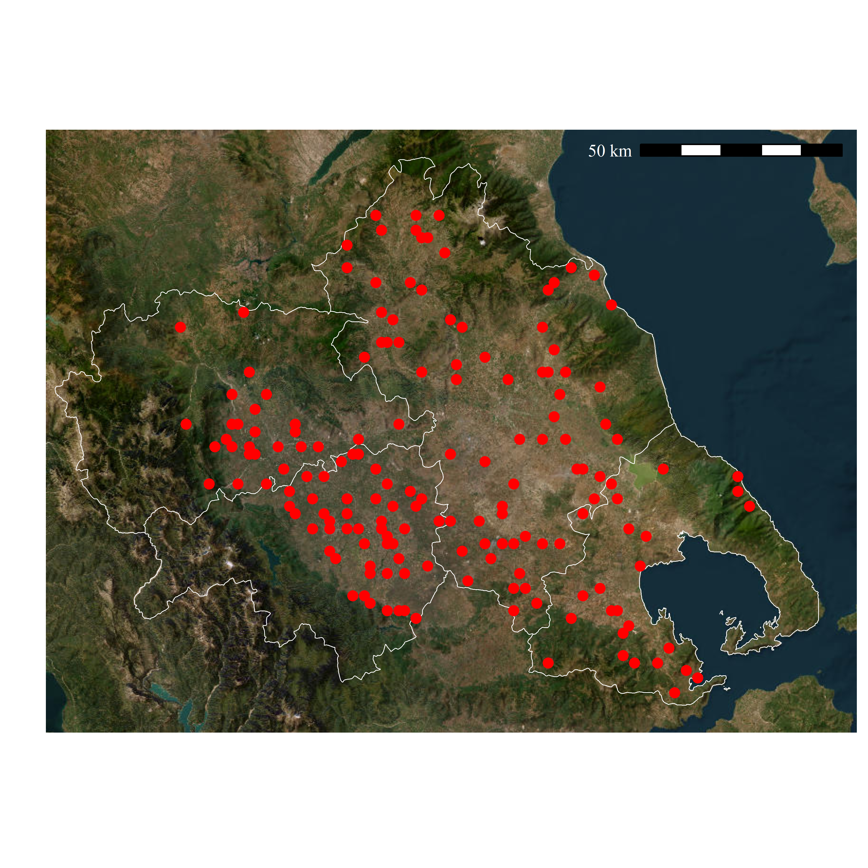
(a) Region of Thessaly within Greece.	(b) The locations of the 168 farms.

Figure 1: The Thessaly region in Greece.

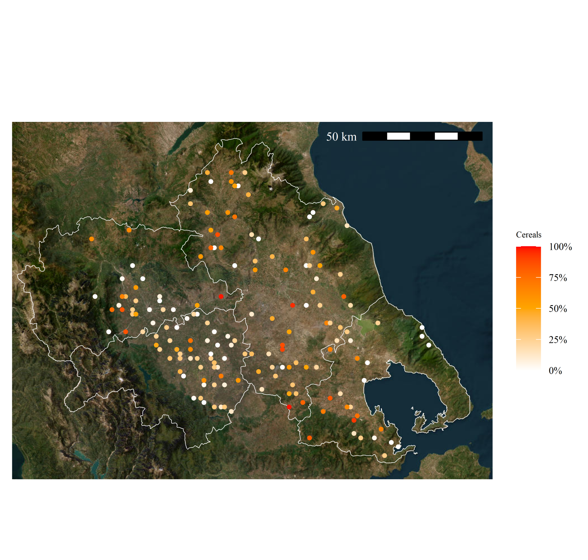
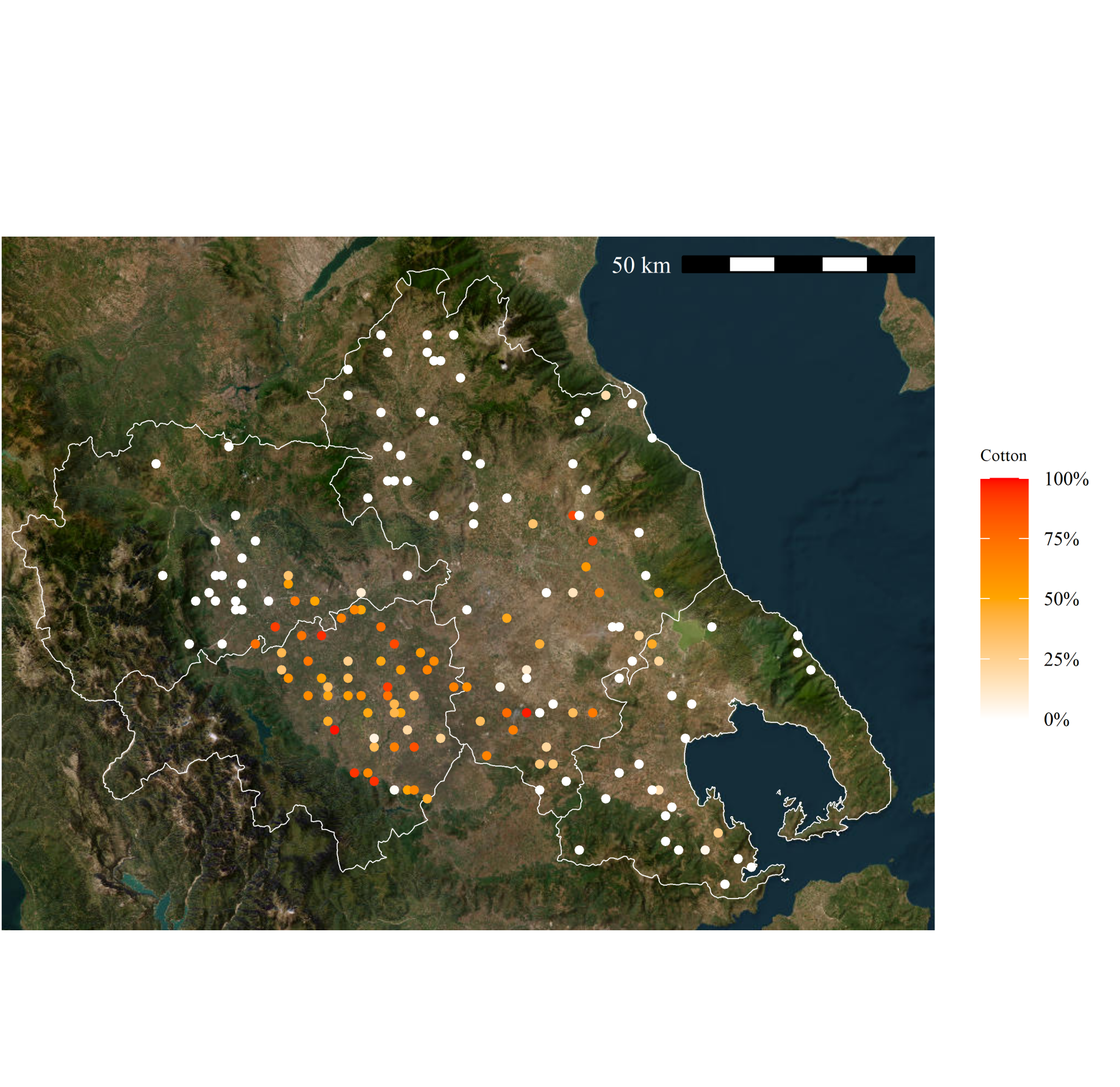
(a) Cereals.	(b) Cotton.
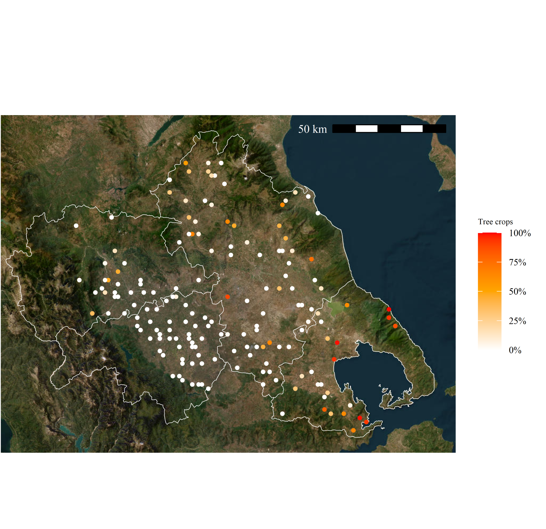
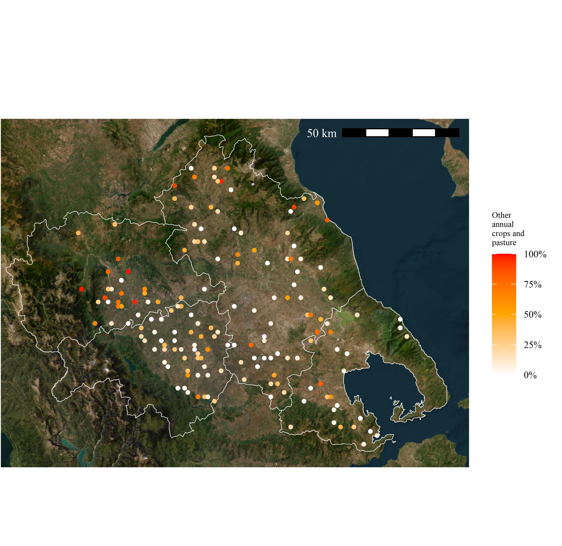
(c) Tree crops.	(d) Other annual crops and pasture.
(e) Grapes and wine.

Figure 2: Heatmaps of the percentages of the cultivated are of the five crops in the Thessaly region.

The goal is to examine the relationship between some known explanatory variables and the composition of the cultivated area. The explanatory variables were the following four

• Human Influence Index (HII, direct human influence on ecosystems). Zero value represents no human influence and 64 represents maximum human influence possible. The index uses all 8 measurements of human presence: Population Density/km², Score of Railroads, Score of Major Roads, Score of Navigable, Rivers, Score of Coastlines, Score of Nighttime Stable Lights Values, Urban Polygons, Land Cover Categories. The range of observed values is $16.08-46.69$, with an average of 29.021.

• The soil pH (CaCl₂). The range of values observed was between $0-6.99$ and the average was 6.33.

• Topsoil organic carbon content (SOC). The content (%) in the surface horizon of soils. The values ranged from 0.54 up to 10.07 with an average equal to 1.41.

• Erosion. The percentage of land downgraded. The sample values spanned between 0.044 and 49.73, with an average equal to 5.60.

5.2 LOOCV for choosing the optimal hyper-parameters

The LOOCV was employed to determine the values of the optimal hyper-parameters in each of the three regression models. To speed-up the computations, 5 values for $\alpha$ were chosen, namely $\alpha=0.1,0.25,0.5,0.75,1$. The bandwidth $h$, hyper-parameter of the GW$\alpha$R was initially set equal to the median of the distances, $h=0.007487129$. Upon experimentation, 10 values spanning from $h/15$ up to $h/10$ were selected.

The optimal value of $\alpha$ for the $\alpha$–regression was 1, while for the $\alpha$–SLX regression model the optimal values were $\alpha=0.25$ and $k=9$. Finally, for the GW$\alpha$R, the optimal values were $\alpha=0.75$ and $h=4.067792\times 10^{-7}$. Using the selected hyper-parameters, the three regression models were run and the produced KLD values were equal to 100.8056 for the $\alpha$–regression model, 160.7815 for the $\alpha$–SLX regression model and 18.1317 for the GW$\alpha$R model.

Table 1 presents the correlations between each pair of components of observed and fitted compositions for each of the three regression models. This is another indication that the GW$\alpha$R model has outperformed the other two competitor, and has fitted the observed compositional data most accurately.

Table 1: Correlations between each component of the observed and fitted compositions for each regression model.

	Cereals	Cotton	Tree crops	Other annual crops	Grapes and wine
Model				and pasture
$\alpha$–regression	0.354	0.587	0.598	0.357	0.353
$\alpha$–SLX	0.333	0.607	0.638	0.371	0.386
GW$\alpha$R	0.896	0.951	0.953	0.874	0.968

Table 2 presents the average marginal effects revealing the effect of each explanatory variable on each component. We remind the marginal effects of each explanatory variable sum to 0 and show the expected change of each of the components at an infinitesimal change in the value of the explanatory variable. The HII has a huge effect, especially on the cerals (positive) and on the other annual crops and pasture (negative). The SOC has the second largest values, while the CaCl₂ and erosion have smaller values.

Table 2: Average marginal effects of each explanatory variable for the GW$\alpha$R model.

	Cereals	Cotton	Tree crops	Other annual crops	Grapes and wine
Model				and pasture
HII	52.815	14.488	13.146	-87.152	6.702
CaCl2	0.056	0.022	-0.022	-0.064	0.008
SOC	-9.024	-2.365	-2.157	14.695	-1.150
Erosion	-1.158	-0.264	-0.502	2.086	-0.161

6 Conclusions

We performed a more detailed examination of the $\alpha$–regression (Tsagris, 2015b, ). We provide the gradient vector and the Hessian matrix in the Appendix. We then expanded this regression model to account for spatial dependencies by introducing the $\alpha$–SLX regression model and the GW$\alpha$R model. For all three regression models formulas for the marginal effects were provided and their capabilities were tested in a real dataset. The results showed that the GW$\alpha$R outperformed the other two.

Future research could explore nonparametric spatially varying models for compositional data, as well as hybrid approaches that blend GWR with machine learning techniques for complex compositional systems.

Appendix: Gradient vector and Hessian matrix for the $\alpha$–regression

The least squares objective function is

$$l(\alpha)=-\frac{1}{2}\text{tr}[(\bm{y}_{\alpha}-\bm{\mu}_{\alpha})^{\top}(\bm{y}_{\alpha}-\bm{\mu}_{\alpha})],$$

where $\bm{y}_{\alpha}$ is the $\alpha$–transformed observed compositional data ($n\times d$ matrix), $\bm{\mu}_{\alpha}$ is the $\alpha$–transformed fitted compositional values ($n\times d$ matrix), $n$ is the number of observations, and $d=D-1$ where $D$ is the number of components in the composition.

The fitted compositional values come from the inverse alr transformation:

$$\mu_{1}=\frac{1}{1+\sum_{j=1}^{d}e^{x^{\top}\beta_{j}}},\quad\mu_{i}=\frac{e^{x^{\top}\beta_{i-1}}}{1+\sum_{j=1}^{d}e^{x^{\top}\beta_{j}}},\quad i=2,\ldots,D.$$

6.1 The $\alpha$–transformation

The $\alpha$–transformation consists of two steps:

Step 1: Power transformation

$$u_{i}=\frac{\mu_{i}^{\alpha}}{\sum_{j=1}^{D}\mu_{j}^{\alpha}},\quad i=1,\ldots,D.$$

Step 2: Helmert transformation

$$z=\frac{1}{\alpha}H(Du-j_{D}),$$

where $H$ is the $d\times D$ Helmert sub-matrix and $j_{D}$ is a $D$-dimensional vector of ones.

6.2 First Derivatives (Gradient)

6.2.1 Main Gradient Formula

$$\frac{\partial l(\alpha)}{\partial\beta_{k}}=\text{tr}\left[(\bm{y}_{\alpha}-\bm{\mu}_{\alpha})^{\top}\frac{\partial\bm{\mu}_{\alpha}}{\partial\beta_{k}}\right].$$

6.2.2 Expanded Gradient Formula

$$\frac{\partial l(\alpha)}{\partial\beta_{k}}=\sum_{i=1}^{n}\sum_{m=1}^{d}\sum_{\ell=1}^{D}\sum_{p=1}^{D}r_{\alpha,im}\cdot\frac{D}{\alpha}H_{m\ell}\cdot\frac{\partial u_{i\ell}}{\partial\mu_{ip}}\cdot\frac{\partial\mu_{ip}}{\partial\beta_{k}}\cdot x_{i},$$

where $r_{\alpha,im}=y_{\alpha,im}-m_{\alpha,im}$ are the residuals in $\alpha$–transformed space, $H_{m\ell}$ is the $(m,\ell)$ element of the Helmert sub-matrix, and $x_{i}$ is the explanatory variable vector for observation $i$.

6.2.3 Jacobian of Power Transformation

$$\frac{\partial u_{i\ell}}{\partial\mu_{ip}}=\begin{cases}\displaystyle\frac{\alpha\mu_{i\ell}^{\alpha-1}}{\sum_{j=1}^{D}\mu_{ij}^{\alpha}}\left(1-\frac{\mu_{i\ell}^{\alpha}}{\sum_{j=1}^{D}\mu_{ij}^{\alpha}}\right)&\text{if }\ell=p\\ [3ex]\displaystyle-\frac{\alpha\mu_{i\ell}^{\alpha}\mu_{ip}^{\alpha-1}}{(\sum_{j=1}^{D}\mu_{ij}^{\alpha})^{2}}&\text{if }\ell\neq p\end{cases}.$$

Let $T_{i}=\sum_{j=1}^{D}\mu_{ij}^{\alpha}$. In compact form:

$$\frac{\partial u_{i\ell}}{\partial\mu_{ip}}=\frac{\alpha\mu_{ip}^{\alpha-1}}{T_{i}}\left(\delta_{\ell p}-\frac{\mu_{i\ell}^{\alpha}}{T_{i}}\right),$$

where $\delta_{\ell p}$ is the Kronecker delta.

6.2.4 Jacobian of Multinomial Logit

Let $S_{i}=1+\sum_{j=1}^{d}e^{x_{i}^{\top}\beta_{j}}$.

$$\frac{\partial\mu_{ip}}{\partial\beta_{k}}=\begin{cases}-\mu_{i1}\mu_{ik}x_{i}&\text{if }p=1\\ \mu_{ik}(1-\mu_{ik})x_{i}&\text{if }p=k+1\\ -\mu_{ip}\mu_{ik}x_{i}&\text{if }p\neq 1,p\neq k+1\end{cases},$$

where $\mu_{ik}=\mu_{i,k+1}$ (the $(k+1)$-th component of the composition).

6.2.5 Vectorized Gradient Formula

$$\frac{\partial l(\alpha)}{\partial\beta_{k}}=X^{\top}w_{k},$$

where the weight vector $w_{k}\in\mathbb{R}^{n}$ has elements:

$$w_{k,i}=\left\{r_{\alpha,i}^{\top}\cdot\frac{D}{\alpha}H\cdot J_{u}(i)\cdot J_{\mu}(i,k)\right\}.$$

Diagonal Contribution

$$w_{k,i}^{\text{diag}}=\sum_{\ell=1}^{D}r_{\alpha,i\ell}H_{\ell}J_{u,\text{diag}}(i,\ell)J_{\mu}(i,\ell,k)$$

where $J_{u,\text{diag}}(i,\ell)=\frac{\alpha\mu_{i\ell}^{\alpha-1}}{T_{i}}\left(1-\frac{\mu_{i\ell}^{\alpha}}{T_{i}}\right)$.

Off-Diagonal Contribution

$$w_{k,i}^{\text{off-diag}}=-\frac{\alpha}{T_{i}^{2}}\left[\left(\sum_{\ell=1}^{D}r_{\alpha,i\ell}H_{\ell}\mu_{i\ell}^{\alpha}\right)\left(\sum_{p=1}^{D}\mu_{ip}^{\alpha-1}J_{\mu}(i,p,k)\right)-\sum_{\ell=1}^{D}r_{\alpha,i\ell}H_{\ell}\mu_{i\ell}^{\alpha}\mu_{i\ell}^{\alpha-1}J_{\mu}(i,\ell,k)\right].$$

Total Weight:

$$w_{k,i}=w_{k,i}^{\text{diag}}+w_{k,i}^{\text{off-diag}}.$$

7 Hessian matrix for the $\alpha$–regression

The sum of squares of the errors is:

$$l(\alpha)=-\frac{1}{2}\sum_{i=1}^{n}\sum_{j=1}^{d}(y_{\alpha,ij}-m_{\alpha,ij})^{2}.$$

We will compute the Hessian matrix including all second-order terms. The gradient is

$$\frac{\partial l(\alpha)}{\partial\beta_{k}}=\sum_{i=1}^{n}\sum_{j=1}^{d}r_{\alpha,ij}\frac{\partial m_{\alpha,ij}}{\partial\beta_{k}},$$

where $r_{\alpha,ij}=y_{\alpha,ij}-m_{\alpha,ij}$. The structure of the Hessian matrix is:

$$H_{\text{exact}}=\begin{bmatrix}H_{1,1}&H_{1,2}&\cdots&H_{1,d}\\ H_{2,1}&H_{2,2}&\cdots&H_{2,d}\\ \vdots&\vdots&\ddots&\vdots\\ H_{d,1}&H_{d,2}&\cdots&H_{d,d}\end{bmatrix}.$$

Each block $H_{k,k^{\prime}}\in\mathbb{R}^{p\times p}$ includes both first and second-order terms.

The derivative with respect to $\beta_{k^{\prime}}$ is:

$$\frac{\partial^{2}l(\alpha)}{\partial\beta_{k}\partial\beta_{k^{\prime}}}=\underbrace{-\sum_{i=1}^{n}\sum_{j=1}^{d}\frac{\partial m_{\alpha,ij}}{\partial\beta_{k}}\frac{\partial m_{\alpha,ij}}{\partial\beta_{k^{\prime}}}}_{\text{First-order term (GN)}}+\underbrace{\sum_{i=1}^{n}\sum_{j=1}^{d}r_{\alpha,ij}\frac{\partial^{2}m_{\alpha,ij}}{\partial\beta_{k}\partial\beta_{k^{\prime}}}}_{\text{Second-order term}}.$$

7.1 First-Order Term (Gauss-Newton Part)

This is identical to the Gauss-Newton approximation:

$$H_{k,k^{\prime}}^{(1)}=-\sum_{i=1}^{n}\sum_{j=1}^{d}\frac{\partial m_{\alpha,ij}}{\partial\beta_{k}}\frac{\partial m_{\alpha,ij}}{\partial\beta_{k^{\prime}}}=-X^{\top}\text{diag}(W_{k,k^{\prime}})X.$$

where

$$W_{k,k^{\prime}}(i,i)=\sum_{j=1}^{d}\frac{\partial m_{\alpha,ij}}{\partial\beta_{k}}\cdot\frac{\partial m_{\alpha,ij}}{\partial\beta_{k^{\prime}}}.$$

7.2 Second-Order Term (Exact Correction)

Computation of $\frac{\partial^{2}m_{\alpha,ij}}{\partial\beta_{k}\partial\beta_{k^{\prime}}}$.

7.2.1 Chain Rule for Second Derivative

The chain rule for first derivative is

$$\frac{\partial m_{\alpha,i}}{\partial\beta_{k}}=\frac{D}{\alpha}H\cdot J_{u}(i)\cdot J_{\mu}(i,k).$$

Taking the derivative with respect to $\beta_{k^{\prime}}$:

$$\frac{\partial^{2}m_{\alpha,i}}{\partial\beta_{k}\partial\beta_{k^{\prime}}}=\frac{D}{\alpha}H\cdot\left[\frac{\partial J_{u}(i)}{\partial\beta_{k^{\prime}}}\cdot J_{\mu}(i,k)+J_{u}(i)\cdot\frac{\partial J_{\mu}(i,k)}{\partial\beta_{k^{\prime}}}\right].$$

7.2.2 Second Derivative of Power Transformation

We need $\frac{\partial J_{u}(i)}{\partial\beta_{k^{\prime}}}$, which involves $\frac{\partial^{2}u_{\ell}}{\partial\mu_{p}\partial\mu_{q}}$. Let $T_{i}=\sum_{j=1}^{D}\mu_{ij}^{\alpha}$.

Diagonal-Diagonal: $\ell=p=q$

$$\frac{\partial^{2}u_{\ell}}{\partial\mu_{\ell}^{2}}=\frac{\alpha(\alpha-1)\mu_{\ell}^{\alpha-2}}{T}\left(1-\frac{\mu_{\ell}^{\alpha}}{T}\right)-\frac{2\alpha^{2}\mu_{\ell}^{2\alpha-2}}{T^{2}}+\frac{2\alpha^{2}\mu_{\ell}^{3\alpha-2}}{T^{3}}.$$

Diagonal-Off-diagonal: $\ell=p\neq q$

$$\frac{\partial^{2}u_{\ell}}{\partial\mu_{\ell}\partial\mu_{q}}=-\frac{\alpha(\alpha-1)\mu_{\ell}^{\alpha-1}\mu_{q}^{\alpha-1}}{T^{2}}\left(1-\frac{\mu_{\ell}^{\alpha}}{T}\right)-\frac{\alpha^{2}\mu_{\ell}^{\alpha}\mu_{q}^{\alpha-1}}{T^{2}}+\frac{2\alpha^{2}\mu_{\ell}^{2\alpha-1}\mu_{q}^{\alpha-1}}{T^{3}}.$$

Off-diagonal-Off-diagonal: $\ell\neq p,\ell=q$

$$\frac{\partial^{2}u_{\ell}}{\partial\mu_{\ell}\partial\mu_{p}}=-\frac{\alpha(\alpha-1)\mu_{\ell}^{\alpha-1}\mu_{p}^{\alpha-1}}{T^{2}}\left(1-\frac{\mu_{\ell}^{\alpha}}{T}\right)-\frac{\alpha^{2}\mu_{\ell}^{2\alpha-1}\mu_{p}^{\alpha-1}}{T^{2}}+\frac{2\alpha^{2}\mu_{\ell}^{3\alpha-1}\mu_{p}^{\alpha-1}}{T^{3}}.$$

Fully Off-diagonal: $\ell\neq p,\ell\neq q,p\neq q$

$$\frac{\partial^{2}u_{\ell}}{\partial\mu_{p}\partial\mu_{q}}=-\frac{\alpha(\alpha-1)\mu_{\ell}^{\alpha}\mu_{p}^{\alpha-2}\delta_{pq}}{T^{2}}-\frac{\alpha^{2}\mu_{\ell}^{\alpha}\mu_{p}^{\alpha-1}\mu_{q}^{\alpha-1}}{T^{2}}+\frac{2\alpha^{2}\mu_{\ell}^{\alpha}\mu_{p}^{\alpha-1}\mu_{q}^{\alpha-1}}{T^{3}},$$

where $\delta_{pq}$ is the Kronecker delta.

7.2.3 General Formula for Hessian of Power Transformation

Let $H_{u}(i,\ell)$ denote the $D\times D$ Hessian matrix for component $\ell$ of $u_{i}$:

$$[H_{u}(i,\ell)]_{pq}=\frac{\partial^{2}u_{i\ell}}{\partial\mu_{ip}\partial\mu_{iq}}.$$

Then:

$$\frac{\partial J_{u}(i)}{\partial\beta_{k^{\prime}}}=\sum_{\ell=1}^{D}\sum_{p=1}^{D}H_{u}(i,\ell)_{pq}\cdot\frac{\partial\mu_{ip}}{\partial\beta_{k^{\prime}}}\cdot e_{\ell}e_{q}^{\top}$$

where $e_{\ell}$ is the $\ell$-th standard basis vector. This becomes a $D\times D$ matrix where each element is:

$$\left[\frac{\partial J_{u}(i)}{\partial\beta_{k^{\prime}}}\right]_{\ell q}=\sum_{p=1}^{D}\frac{\partial^{2}u_{i\ell}}{\partial\mu_{ip}\partial\mu_{iq}}\cdot\frac{\partial\mu_{ip}}{\partial\beta_{k^{\prime}}}.$$

7.2.4 Second Derivative of Multinomial Logit

We need $\frac{\partial J_{\mu}(i,k)}{\partial\beta_{k^{\prime}}}$, which involves $\frac{\partial^{2}\mu_{ip}}{\partial\beta_{k}\partial\beta_{k^{\prime}}}$. Let $\mu_{ik}=\mu_{i,k+1}$ and $\mu_{ik^{\prime}}=\mu_{i,k^{\prime}+1}$.

For component $p=1$ (reference):

$$\frac{\partial^{2}\mu_{i1}}{\partial\beta_{k}^{2}}=\mu_{i1}\mu_{ik}(\mu_{ik}-\mu_{i1})x_{i}x_{i}^{\top}.$$

For component $p=k+1$:

$$\frac{\partial^{2}\mu_{i,k+1}}{\partial\beta_{k}^{2}}=\mu_{ik}(1-\mu_{ik})(1-2\mu_{ik})x_{i}x_{i}^{\top}.$$

For other components $p\neq 1,p\neq k+1$:

$$\frac{\partial^{2}\mu_{ip}}{\partial\beta_{k}^{2}}=\mu_{ip}\mu_{ik}(\mu_{ik}+\mu_{ip})x_{i}x_{i}^{\top}.$$

Case 2: $k\neq k^{\prime}$ (Different Components)

For component $p=1$ (reference):

$$\frac{\partial^{2}\mu_{i1}}{\partial\beta_{k}\partial\beta_{k^{\prime}}}=\mu_{i1}\mu_{ik}\mu_{ik^{\prime}}x_{i}x_{i}^{\top}.$$

For component $p=k+1$:

$$\frac{\partial^{2}\mu_{i,k+1}}{\partial\beta_{k}\partial\beta_{k^{\prime}}}=-\mu_{ik}\mu_{ik^{\prime}}(1-\mu_{ik})x_{i}x_{i}^{\top}.$$

For component $p=k^{\prime}+1$:

$$\frac{\partial^{2}\mu_{i,k^{\prime}+1}}{\partial\beta_{k}\partial\beta_{k^{\prime}}}=-\mu_{ik^{\prime}}\mu_{ik}(1-\mu_{ik^{\prime}})x_{i}x_{i}^{\top}.$$

For other components $p\neq 1,k+1,k^{\prime}+1$:

$$\frac{\partial^{2}\mu_{ip}}{\partial\beta_{k}\partial\beta_{k^{\prime}}}=\mu_{ip}\mu_{ik}\mu_{ik^{\prime}}x_{i}x_{i}^{\top}.$$

7.2.5 Assembling the Second-Order Term

The second-order correction to the Hessian is:

$$H_{k,k^{\prime}}^{(2)}=\sum_{i=1}^{n}\sum_{j=1}^{d}r_{\alpha,ij}\frac{\partial^{2}m_{\alpha,ij}}{\partial\beta_{k}\partial\beta_{k^{\prime}}},$$

where

$$\frac{\partial^{2}m_{\alpha,ij}}{\partial\beta_{k}\partial\beta_{k^{\prime}}}=[H]_{j}\cdot\left[\frac{\partial J_{u}(i)}{\partial\beta_{k^{\prime}}}\cdot J_{\mu}(i,k)+J_{u}(i)\cdot\frac{\partial J_{\mu}(i,k)}{\partial\beta_{k^{\prime}}}\right]\cdot\frac{D}{\alpha}.$$

Here $[H]_{j}$ denotes the $j$-th row of the Helmert matrix.

Explicit Form

$$H_{k,k^{\prime}}^{(2)}=\sum_{i=1}^{n}r_{\alpha,i}^{\top}\cdot\frac{D}{\alpha}H\cdot\left[\sum_{p=1}^{D}\left(\sum_{\ell,q}H_{u}(i,\ell,p,q)\frac{\partial\mu_{ip}}{\partial\beta_{k^{\prime}}}\right)J_{\mu}(i,k)_{q}e_{\ell}e_{q}^{\top}+J_{u}(i)\cdot\frac{\partial^{2}\mu}{\partial\beta_{k}\partial\beta_{k^{\prime}}}x_{i}x_{i}^{\top}\right].$$

7.3 Complete Hessian (Exact)

$$H_{k,k^{\prime}}=H_{k,k^{\prime}}^{(1)}+H_{k,k^{\prime}}^{(2)}=-X^{\top}\text{diag}(W_{k,k^{\prime}}^{(1)})X+\sum_{i=1}^{n}r_{\alpha,i}^{\top}\cdot S_{k,k^{\prime}}(i)\cdot x_{i}x_{i}^{\top},$$

where $W_{k,k^{\prime}}^{(1)}$ are the Gauss-Newton weights and $S_{k,k^{\prime}}(i)$ is the second-order correction tensor for observation $i$.

References

- Aitchison, (2003) Aitchison, J. (2003). The statistical analysis of compositional data. New Jersey: Reprinted by The Blackburn Press.
- Alenazi, (2022) Alenazi, A. (2022). f-divergence and parametric regression models for compositional data. Pakistan Journal of Statistics and Operation Research, 18(4):867–882.
- Amemiya, (1985) Amemiya, T. (1985). Advanced Econometrics. Harvard University Press, Cambridge, MA.
- Baxter, (2001) Baxter, M. (2001). Statistical modelling of artefact compositional data. Archaeometry, 43(1):131–147.
- Baxter et al., (2005) Baxter, M., Beardah, C., Cool, H., and Jackson, C. (2005). Compositional data analysis of some alkaline glasses. Mathematical geology, 37(2):183–196.
- Brunsdon et al., (1996) Brunsdon, C., Fotheringham, A. S., and Charlton, M. E. (1996). Geographically weighted regression: a method for exploring spatial nonstationarity. Geographical Analysis, 28(4):281–298.
- Chen and Li, (2016) Chen, E. Z. and Li, H. (2016). A two-part mixed-effects model for analyzing longitudinal microbiome compositional data. Bioinformatics, 32(17):2611–2617.
- Clarotto et al., (2022) Clarotto, L., Allard, D., and Menafoglio, A. (2022). A new class of -transformations for the spatial analysis of compositional data. Spatial Statistics, 47:100570.
- Egozcue et al., (2003) Egozcue, J., Pawlowsky-Glahn, V., Mateu-Figueras, G., and Barceló-Vidal, C. (2003). Isometric logratio transformations for compositional data analysis. Mathematical Geology, 35(3):279–300.
- Elhorst, (2014) Elhorst, J. P. (2014). Spatial Econometrics: From Cross-Sectional Data to Spatial Panels. SpringerBriefs in Regional Science. Springer, Heidelberg.
- Elzhov et al., (2023) Elzhov, T. V., Mullen, K. M., Spiess, A.-N., and Bolker, B. (2023). minpack.lm: R Interface to the Levenberg-Marquardt Nonlinear Least-Squares Algorithm Found in MINPACK, Plus Support for Bounds. R package version 1.2-4.
- Fotheringham et al., (2002) Fotheringham, A. S., Brunsdon, C., and Charlton, M. (2002). Geographically Weighted Regression: The Analysis of Spatially Varying Relationships. John Wiley & Sons, Chichester, UK.
- Gallant, (1987) Gallant, A. R. (1987). Nonlinear Statistical Models. Wiley, New York.
- Gretton et al., (2012) Gretton, A., Borgwardt, K. M., Rasch, M. J., Schölkopf, B., and Smola, A. (2012). A Kernel Two-Sample Test. Journal of Machine Learning Research, 13(1):723–773.
- Gueorguieva et al., (2008) Gueorguieva, R., Rosenheck, R., and Zelterman, D. (2008). Dirichlet component regression and its applications to psychiatric data. Computational Statistics & Data Analysis, 52(12):5344–5355.
- Hijazi and Jernigan, (2009) Hijazi, R. H. and Jernigan, R. W. (2009). Modelling compositional data using Dirichlet regression models. Journal of Applied Probability & Statistics, 4(1):77–91.
- Iyengar and Dey, (2002) Iyengar, M. and Dey, D. K. (2002). A semiparametric model for compositional data analysis in presence of covariates on the simplex. Test, 11(2):303–315.
- Jennrich, (1969) Jennrich, R. I. (1969). Asymptotic properties of nonlinear least squares estimators. Annals of Mathematical Statistics, 40(2):633–643.
- Katz and King, (1999) Katz, J. and King, G. (1999). A statistical model for multiparty electoral data. American Political Science Review, pages 15–32.
- Leininger et al., (2013) Leininger, T. J., Gelfand, A. E., Allen, J. M., and Silander Jr, J. A. (2013). Spatial Regression Modeling for Compositional Data With Many Zeros. Journal of Agricultural, Biological, and Environmental Statistics, 18(3):314–334.
- LeSage and Pace, (2009) LeSage, J. P. and Pace, R. K. (2009). Introduction to Spatial Econometrics. Chapman and Hall/CRC, Boca Raton, FL.
- Mardia and Jupp, (2000) Mardia, K. and Jupp, P. (2000). Directional Statistics. London: John Wiley & Sons.
- Mattas et al., (2025) Mattas, K., Tsagris, M., and Tzouvelekas, V. (2025). Using synthetic farm data to estimate individual nitrate leaching levels. American Journal of Agricultural Economics, Forthcoming.
- Melo et al., (2009) Melo, T. F., Vasconcellos, K. L., and Lemonte, A. J. (2009). Some restriction tests in a new class of regression models for proportions. Computational Statistics & Data Analysis, 53(12):3972–3979.
- Morais et al., (2018) Morais, J., Thomas-Agnan, C., and Simioni, M. (2018). Using compositional and Dirichlet models for market share regression. Journal of Applied Statistics, 45(9):1670–1689.
- Mullahy, (2015) Mullahy, J. (2015). Multivariate fractional regression estimation of econometric share models. Journal of Econometric Methods, 4(1):71–100.
- Murteira and Ramalho, (2016) Murteira, J. M. R. and Ramalho, J. J. S. (2016). Regression analysis of multivariate fractional data. Econometric Reviews, 35(4):515–552.
- Otero et al., (2005) Otero, N., Tolosana-Delgado, R., Soler, A., Pawlowsky-Glahn, V., and Canals, A. (2005). Relative vs. absolute statistical analysis of compositions: A comparative study of surface waters of a Mediterranean river. Water research, 39(7):1404–1414.
- Scealy and Welsh, (2011) Scealy, J. and Welsh, A. (2011). Regression for compositional data by using distributions defined on the hypersphere. Journal of the Royal Statistical Society. Series B, 73(3):351–375.
- Schrab et al., (2023) Schrab, A., Kim, I., Albert, M., Laurent, B., Guedj, B., and Gretton, A. (2023). MMD aggregated two-sample test. Journal of Machine Learning Research, 24(194):1–81.
- Shi et al., (2016) Shi, P., Zhang, A., Li, H., et al. (2016). Regression analysis for microbiome compositional data. The Annals of Applied Statistics, 10(2):1019–1040.
- (32) Tsagris, M. (2015a). A novel, divergence based, regression for compositional data. In Proceedings of the 28th Panhellenic Statistics Conference, April, Athens, Greece.
- (33) Tsagris, M. (2015b). Regression analysis with compositional data containing zero values. Chilean Journal of Statistics, 6(2):47–57.
- Tsagris et al., (2025) Tsagris, M., Athineou, G., Alenazi, A., and Adam, C. (2025). Compositional: Compositional Data Analysis. R package version 7.9.
- Tsagris et al., (2011) Tsagris, M., Preston, S., and Wood, A. (2011). A data-based power transformation for compositional data. In Proceedings of the 4rth Compositional Data Analysis Workshop, Girona, Spain.
- Tsagris et al., (2016) Tsagris, M., Preston, S., and Wood, A. T. (2016). Improved classification for compositional data using the -transformation. Journal of Classification, 33(2):243–261.
- Tsagris and Stewart, (2018) Tsagris, M. and Stewart, C. (2018). A Dirichlet regression model for compositional data with zeros. Lobachevskii Journal of Mathematics, 39(3):398–412.
- Tsagris and Stewart, (2020) Tsagris, M. and Stewart, C. (2020). A folded model for compositional data analysis. Australian & New Zealand Journal of Statistics, 62(2):249–277.
- Wu, (1981) Wu, C. F. J. (1981). Asymptotic theory of nonlinear least squares estimation. Annals of Statistics, 9(3):501–513.
- Xia et al., (2013) Xia, F., Chen, J., Fung, W. K., and Li, H. (2013). A logistic normal multinomial regression model for microbiome compositional data analysis. Biometrics, 69(4):1053–1063.
- Yoshida et al., (2021) Yoshida, T., Murakami, D., Seya, H., Tsutsumida, N., and Nakaya, T. (2021). Geographically weighted regression for compositional data: An application to the US household income compositions. In Proceedings of the 11th International Conference on Geographic Information Science.