hoppet v2 release note

Abstract

We document the three main new features in the v2 release series of the hoppet parton distribution function evolution code, specifically support for N³LO QCD evolution in the variable flavour number scheme, for the determination of hadronic structure functions for massless quarks up to N³LO, and for QED evolution to an accuracy phenomenologically equivalent to NNLO QCD. Additionally we describe a new Python interface, CMake build option, functionality to save a hoppet table as an LHAPDF grid and update our performance benchmarks, including optimisations in interpolating PDF tables.

margin=25mm, headheight=110pt, footskip=30pt

CERN-TH-2023-237

MPP-2023-285

OUTP-23-15P

[1]organization=CERN, Theoretical Physics Department, postcode=CH-1211 ,city=Geneva 23, country=Switzerland [2]organization=INFN, Sezione di Milano-Bicocca, and Universita di Milano-Bicocca, Piazza della Scienza 3, postcode=20126 ,city=Milano, country=Italy [3]organization=Rudolf Peierls Centre for Theoretical Physics, Clarendon Laboratory, Parks Road, postcode=OX1 3PU ,city=Oxford, country=UK [4]organization=All Souls College, postcode=OX1 4AL ,city=Oxford, country=UK [5]organization=Max-Planck-Institut fur Physik, Boltzmannstr. 8, postcode=85748 ,city=Garching, country=Germany [6]organization=Physik-Department, Technische Universitat Munchen, James-Franck-Strasse 1, postcode=85748 ,city=Garching, country=Germany [7]organization=Prescient Design, Genentech, 149 5th Avenue,city=New York, postcode=NY 10010, country=USA

1 Introduction

hoppet Salam:2008qg is a parton distribution function (PDF) evolution code written in modern Fortran, with interfaces also for C/C++ and earlier dialects of Fortran. It offers both a high-level PDF evolution interface and user-access to lower-level functionality for operations such as convolutions of coefficient functions and PDFs. It is designed to provide flexible, fast and accurate evolution.

Since the first major release of hoppet, the landscape of PDF evolution codes has evolved substantially, with a range of new open-source codes having been developed, for example the APFEL Bertone:2013vaa , APFEL++ Bertone:2017gds and EKO Candido:2022tld codes (the latter including features such as cached evolution that have long been standard in hoppet). Nevertheless, hoppet remains a powerful tool, notably for its ability to reach high and quantifiable accuracies with competitive speed. As a result it often provides a critical reference for benchmark studies, as those presented e.g. in Refs. Dittmar:2005ed , Bertone:2024dpm . It also provides the option of fast (millisecond-scale) evolution with accuracies $\sim 10^{-4}$, which is more than sufficient for phenomenological applications. Furthermore its exposition not just of full PDF evolution Lai:2010vv , Gao:2013xoa , Butterworth:2015oua , PDF4LHCWorkingGroup:2022cjn but also of low-level functionality makes it useful for a range of fixed-order Caola:2019nzf , Asteriadis:2019dte , Bargiela:2022dla , all-order Banfi:2010xy , Dasgupta:2014yra , Banfi:2015pju , Monni:2016ktx , Bizon:2017rah , Buonocore:2024xmy and Monte Carlo Monni:2019whf , vanBeekveld:2023ivn , Buonocore:2024pdv , vanBeekveld:2025lpz applications. With the advent of ever more precise data from the LHC at CERN, and future very high precision data at the forthcoming Electron-Ion Collider AbdulKhalek:2021gbh at Brookhaven National Laboratory, the continued development of tools such as hoppet remains important for the field.

This release note documents three major additions to hoppet, made available as part of release 2.0.0: (1) support for QCD evolution at N³LO in the (zero mass) variable flavour number scheme (VFNS) Buza:1996wv (Section 2); (2) support for the determination of massless hadronic structure functions, as initially developed for calculations of vector-boson fusion, and later deep inelastic scattering, cross sections Cacciari:2015jma , Dreyer:2016oyx , Dreyer:2018qbw , Dreyer:2018rfu , Karlberg:2024hnl (Section 3); (3) support for QED evolution (Section 4), originally developed as part of the LuxQED project for the evaluation of the photon density inside a proton and its extension to lepton distributions in the proton Manohar:2016nzj , Manohar:2017eqh , Buonocore:2020nai , Buonocore:2021bsf .

This release also includes a range of other additions relative to the original 1.1.0 release documented in Salam:2008qg , in particular a Python interface (Section 5), a CMake-based build system (Section 6), and the ability to write LHAPDF grids (Section 7). We have also updated the performance benchmarks and improved the speed for interpolating PDF tables also when loaded from LHAPDF (Section 8). hoppet can be obtained by executing

⬇

git clone https://github.com/hoppet-code/hoppet.git

Unified documentation of the whole hoppet package is part of the distribution at https://github.com/hoppet-code/hoppet in the doc/ directory. Details of the other changes since release 1.1.0 can be found in the NEWS.md and ChangeLog files from the repository.

Note that as of the 2.0.0 release, hoppet’s library name has been renamed from hoppet_v1 to hoppet, and similarly for the main module and C++ include file. Users with an existing installation of hoppet (v1) should make sure that they link with the new library name.

2 QCD evolution at N³LO

In recent years significant progress in determining the perturbative components needed for unpolarised QCD evolution at N³LO has been made (cf. A for technical details on the evolution at N³LO). This has now reached the stage that two PDF groups have released fits at approximate N³LO (aN³LO) accuracy McGowan:2022nag , NNPDF:2024nan along with their combination in Ref. Cridge:2024icl . Of the three contributions that are needed at full N³LO accuracy only two are fully known. In particular the four-loop $\beta$-function vanRitbergen:1997va , Czakon:2004bu and associated mass thresholds Chetyrkin:1997sg have been known for a very long time. On the other hand the intricate calculations of the three-loop matching relations needed for both the single and two mass VFNS were only very recently completed Bierenbaum:2009mv , Ablinger:2010ty , Kawamura:2012cr , Blumlein:2012vq , ABLINGER2014263 , Ablinger:2014nga , Ablinger:2014vwa , Behring:2014eya , Ablinger:2019etw , Behring:2021asx , Ablinger:2023ahe , Ablinger:2024xtt , Ablinger:2025awb . Finally the four-loop splitting functions entering the DGLAP equation are currently not known exactly, except for certain $n_{f}$-dependent terms Gracey:1994nn , Davies:2016jie , Moch:2017uml , Gehrmann:2023cqm , Falcioni:2023tzp , Gehrmann:2023iah , Kniehl:2025ttz . However, enough Mellin-moments have been computed that together with the exact pieces just mentioned and known small- and large-$x$ behaviours, approximate splitting functions suitable for phenomenology can be reliably determined McGowan:2022nag , NNPDF:2024nan , Moch:2021qrk , Falcioni:2023luc , Falcioni:2023vqq , Moch:2023tdj , Falcioni:2024xyt , Falcioni:2024qpd . We have therefore incorporated the aforementioned pieces, using code that is publicly available with those references, with the intention of updating the splitting functions as they become more precisely known.

2.1 Interface

For the specific implementation in hoppet version 2.0.0 we rely on the approximations computed in Refs. Davies:2016jie , Moch:2017uml , Falcioni:2023luc , Falcioni:2023vqq , Moch:2023tdj , Falcioni:2024xyt , Falcioni:2024qpd (FHMPRUVV), the implementation of the three-loop (single-mass) VFNS coefficients as found in Ref. BlumleinCode , which contains code associated with Refs. Ablinger:2024xtt , Fael:2022miw and our own implementation of the four-loop running coupling. Since the implementation here extends core features of hoppet that were already available in version 1.1.0, very little is needed on the side of the user to invoke the evolution. Most importantly all routines that take an nloop argument, e.g. InitDglapHolder, InitRunningCoupling, hoppetStart, and hoppetEval now support nloop = 4. The user also has a few choices they can make in terms of the splitting functions used. The approximate splitting functions can return three different choices corresponding to upper and lower edges of an uncertainty band and their average. The user can control which one to use by setting the n3lo_splitting_variant variable in the dglap_choices module. Allowed values are n3lo_splitting_Nfitav (default), n3lo_splitting_Nfiterr1, or n3lo_splitting_Nfiterr2. When the exact splitting functions become available they will correspond to n3lo_splitting_exact. Similarly if a set of parametrisations of the exact splitting functions become available they will correspond to n3lo_splitting_param.

It is expected that more precise approximations will become available in the future. The user can control which series of approximation to use, again by setting a variable in dglap_choices, called n3lo_splitting_approximation. By default it is set to the most recent set of approximations by the FHMPRUVV group. At the time of writing it can take one of three values:

• n3lo_splitting_approximation_up_to_2310_05744, with the approximations in papers up to and including Ref. Moch:2023tdj ;

• n3lo_splitting_approximation_up_to_2404_09701, with the approximations in papers up to and including Ref. Falcioni:2024xyt ;

• n3lo_splitting_approximation_up_to_2410_08089, the default value at the time of writing, with the approximations in papers up to and including Ref. Falcioni:2024qpd .

Besides the splitting functions, we have also incorporated the single-mass thresholds up to N³LO, as calculated in Refs. Bierenbaum:2009mv , Ablinger:2010ty , Kawamura:2012cr , Blumlein:2012vq , ABLINGER2014263 , Ablinger:2014nga , Ablinger:2014vwa , Behring:2014eya , Ablinger:2019etw , Behring:2021asx , Ablinger:2023ahe , Ablinger:2024xtt . As of version 2.1.0, the N³LO thresholds are available in two forms, using code from Refs. BlumleinCode , Fael:2022miw . One can choose which form to use by setting the n3lo_nfthreshold variable to one of

• n3lo_nfthreshold_libOME: this uses piecewise high-order Laurent-series expansions in different regions of $x$, with a stated accuracy of at least $2048\epsilon$ where $\epsilon$ is the precision of a 64-bit real variable. It relies on the libome C++ library from https://gitlab.com/libome/libome. Initialisation time is below $1\,\text{s}$. This is the default choice.

• n3lo_nfthreshold_exact_fortran: all contributions are exact, except for the $A_{\text{hg}}^{\text{S}}$ term in Eq. (A), which is based on piecewise expansions. The exact contributions make extensive use of hplog5 FortranPolyLog calls and lead to an initialisation time of $10{-}30\,\text{s}$. The piecewise expansions for $A_{\text{hg}}^{\text{S}}$ are less accurate than with the n3lo_nfthreshold_libOME choice.

2.2 Reference results

In Table 1 we show the results of the full N³LO evolution in the VFNS, using the most up-to-date perturbative input at the time of writing this release note. To assess the evolution we take the initial condition of Ref. Dittmar:2005ed at an initial scale $\sqrt{2}~\text{GeV}$ and $n_{f}=3$. We evolve to $Q=100~\text{GeV}$. The numbers are obtained using parametrised NNLO splitting functions, but exact mass thresholds at this order. The table has been generated with $\texttt{dy}=0.05$, $\texttt{dlnlnQ}=\text{dy/4}$. Increasing $\texttt{dy}=0.10$ leaves the results unchanged at the precision shown, while going to $\texttt{dy}=0.20$ for higher speed would change the results by a relative amount below $10^{-4}$.

Table 1 cannot be directly compared to the benchmarking tables of Ref. Cooper-Sarkar:2024crx because they do not include the mass thresholds in the N³LO evolution. To facilitate comparisons we therefore additionally provide Table 2, corresponding to fixed-flavour ($n_{f}=4$) evolution, with the choice of n3lo_splitting_approximation_up_to_2310_05744. Of the MSHT and NNPDF results, the NNPDF results (Table 2 of Ref. Cooper-Sarkar:2024crx ) are closer to ours.

The results in both tables can be regenerated with the help of the following script, which uses the Python interface of Section 5: benchmarking/tabulation_crosscheck_2406_16188.py.

$x$	$u-\bar{u}$	$d-\bar{d}$	$\bar{d}-\bar{u}$	$2(\bar{u}+\bar{d})$	$s+\bar{s}$	$c+\bar{c}$	$b+\bar{b}$	$g$
$10^{-7}$	$1.0589^{-4}$	$4.8664^{-5}$	$8.1967^{-6}$	$1.6234^{+2}$	$8.0100^{+1}$	$7.7207^{+1}$	$6.5254^{+1}$	$1.1238^{+3}$
$10^{-6}$	$5.9691^{-4}$	$3.2634^{-4}$	$3.3146^{-5}$	$7.6786^{+1}$	$3.7544^{+1}$	$3.5836^{+1}$	$2.9889^{+1}$	$5.1159^{+2}$
$10^{-5}$	$3.0235^{-3}$	$1.7532^{-3}$	$1.3081^{-4}$	$3.5436^{+1}$	$1.7044^{+1}$	$1.6106^{+1}$	$1.3142^{+1}$	$2.2224^{+2}$
$10^{-4}$	$1.4079^{-2}$	$8.2354^{-3}$	$4.9511^{-4}$	$1.5611^{+1}$	$7.2731^{+0}$	$6.7862^{+0}$	$5.3294^{+0}$	$8.8594^{+1}$
$10^{-3}$	$6.0849^{-2}$	$3.5086^{-2}$	$1.7751^{-3}$	$6.3823^{+0}$	$2.7798^{+0}$	$2.5204^{+0}$	$1.8516^{+0}$	$3.0349^{+1}$
$10^{-2}$	$2.3361^{-1}$	$1.3074^{-1}$	$5.8324^{-3}$	$2.2673^{+0}$	$8.5415^{-1}$	$7.0444^{-1}$	$4.6228^{-1}$	$7.7859^{+0}$
$0.1$	$5.4846^{-1}$	$2.6950^{-1}$	$9.9965^{-3}$	$3.8453^{-1}$	$1.1248^{-1}$	$6.8296^{-2}$	$3.7899^{-2}$	$8.4964^{-1}$
$0.3$	$3.4441^{-1}$	$1.2761^{-1}$	$2.9457^{-3}$	$3.4575^{-2}$	$8.8873^{-3}$	$3.9659^{-3}$	$2.0846^{-3}$	$7.8697^{-2}$
$0.5$	$1.1790^{-1}$	$3.0597^{-2}$	$3.6526^{-4}$	$2.3206^{-3}$	$5.6808^{-4}$	$2.0185^{-4}$	$1.1382^{-4}$	$7.6337^{-3}$
$0.7$	$1.9329^{-2}$	$2.9648^{-3}$	$1.2848^{-5}$	$5.2429^{-5}$	$1.2662^{-5}$	$3.4020^{-6}$	$2.4956^{-6}$	$3.7094^{-4}$
$0.9$	$3.3153^{-4}$	$1.6737^{-5}$	$8.0961^{-9}$	$2.5214^{-8}$	$6.6432^{-9}$	$7.6153^{-10}$	$1.4323^{-9}$	$1.1716^{-6}$

Table 1: N³LO evolution of the initial condition given in Section 4.4 of Ref. Dittmar:2005ed , using the same notation where $a\cdot 10^{b}=a^{b}$. The evolution is performed taking the initial condition at $\sqrt{2}~\text{GeV}$ (just below the charm mass) and evolving in the VFNS up to $Q=100~\text{GeV}$, with a charm-quark pole mass of $1.414213563\;\mathrm{GeV}$ and a bottom-quark pole mass of $4.5\;\mathrm{GeV}$. The NNLO splitting functions are the parametrised form (nnlo_splitting_variant = nnlo_splitting_param), to facilitate comparisons by other groups, and the N³LO splitting functions use the n3lo_splitting_approximation = n3lo_splitting_approximation_up_to_2410_08089 choice.

$x$	$u-\bar{u}$	$d-\bar{d}$	$\bar{d}-\bar{u}$	$2(\bar{u}+\bar{d})$	$s-\bar{s}$	$s+\bar{s}$	$c+\bar{c}$	$g$
$10^{-7}$	$9.8370^{-5}$	$4.5171^{-5}$	$7.5013^{-6}$	$1.4888^{+2}$	$-2.9105^{-5}$	$7.3368^{+1}$	$7.2653^{+1}$	$1.0851^{+3}$
$10^{-6}$	$5.6405^{-4}$	$3.0895^{-4}$	$3.0730^{-5}$	$7.1925^{+1}$	$-4.6739^{-5}$	$3.5111^{+1}$	$3.4544^{+1}$	$5.0392^{+2}$
$10^{-5}$	$2.8946^{-3}$	$1.6810^{-3}$	$1.2302^{-4}$	$3.3868^{+1}$	$-3.5766^{-6}$	$1.6258^{+1}$	$1.5808^{+1}$	$2.2292^{+2}$
$10^{-4}$	$1.3633^{-2}$	$7.9832^{-3}$	$4.7274^{-4}$	$1.5188^{+1}$	$\phantom{-}2.1123^{-4}$	$7.0599^{+0}$	$6.7033^{+0}$	$9.0268^{+1}$
$10^{-3}$	$5.9567^{-2}$	$3.4382^{-2}$	$1.7232^{-3}$	$6.3028^{+0}$	$\phantom{-}3.9314^{-4}$	$2.7387^{+0}$	$2.4621^{+0}$	$3.1350^{+1}$
$10^{-2}$	$2.3130^{-1}$	$1.2962^{-1}$	$5.7645^{-3}$	$2.2675^{+0}$	$-1.9644^{-4}$	$8.5255^{-1}$	$6.6402^{-1}$	$8.1568^{+0}$
$0.1$	$5.5131^{-1}$	$2.7140^{-1}$	$1.0085^{-2}$	$3.8980^{-1}$	$-3.1812^{-4}$	$1.1388^{-1}$	$5.9843^{-2}$	$9.0615^{-1}$
$0.3$	$3.5044^{-1}$	$1.3015^{-1}$	$3.0145^{-3}$	$3.5426^{-2}$	$-3.8409^{-5}$	$9.0900^{-3}$	$3.3507^{-3}$	$8.4431^{-2}$
$0.5$	$1.2112^{-1}$	$3.1518^{-2}$	$3.7779^{-4}$	$2.3973^{-3}$	$-3.3053^{-6}$	$5.8501^{-4}$	$1.7709^{-4}$	$8.1568^{-3}$
$0.7$	$2.0078^{-2}$	$3.0889^{-3}$	$1.3448^{-5}$	$5.4598^{-5}$	$-1.1810^{-8}$	$1.3105^{-5}$	$3.6963^{-6}$	$3.9248^{-4}$
$0.9$	$3.5128^{-4}$	$1.7793^{-5}$	$8.6472^{-9}$	$2.6378^{-8}$	$-1.5848^{-10}$	$6.8222^{-9}$	$2.6776^{-9}$	$1.2262^{-6}$

Table 2: N³LO evolution of the initial condition given in Section 4.4 of Ref. Dittmar:2005ed , using the same notation where $a\cdot 10^{b}=a^{b}$. The evolution is performed taking the initial condition at $\sqrt{2}~\text{GeV}$ (just below the charm mass) and evolving in the FFN scheme ($n_{f}=4$) up to $Q=100~\text{GeV}$. The NNLO splitting functions are the parametrised form (nnlo_splitting_variant = nnlo_splitting_param), to facilitate comparisons by other groups, and the N³LO splitting functions use the n3lo_splitting_approximation = n3lo_splitting_approximation_up_to_2310_05744 choice. This table can be directly compared to tables 1 and 2 in Ref. Cooper-Sarkar:2024crx

(a)

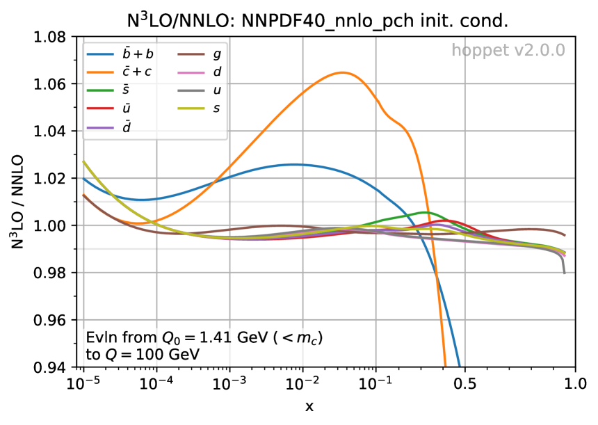
(b)

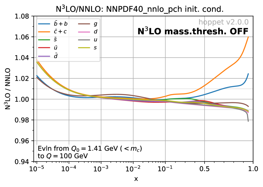
(c)

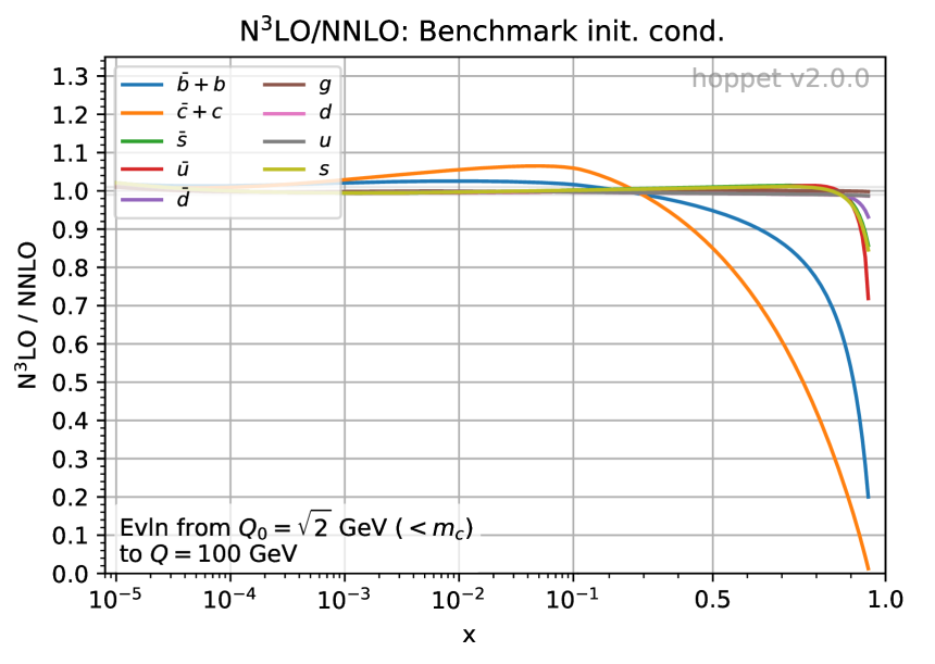
(d)

Figure 1: Ratio of the PDFs at $100\;\mathrm{GeV}$ with N³LO evolution versus NNLO evolution. The evolution starts from the same initial condition at NNLO and N³LO, at an initial scale $Q_{0}\simeq 1.41\;\mathrm{GeV}$. In the upper plots, we use the standard benchmark initial condition. In the lower plots, the initial condition is the NNPDF40_pch_nnlo_as_01180 PDF NNPDF:2021njg at $Q_{0}$. The left-hand plots show the ratio with N³LO evolution including N³LO mass thresholds, while the right-hand plots show the evolution without the N³LO mass thresholds. In all cases, the N³LO evolution uses n3lo_splitting_approximation_up_to_2410_08089.

We close this section by illustrating the impact of N³LO versus NNLO evolution, Fig. 1. Let us first focus on the top-left plot, Fig. 1(a). We start with the benchmark initial condition at the standard low scale of $Q_{0}=\sqrt{2}\;\mathrm{GeV}$, just below a charm mass of $m_{c}=1.414213563\;\mathrm{GeV}$, so as to ensure that the evolution starts with $n_{f}=3$. We then evolve the PDF separately with N³LO and NNLO evolution, and show the N³LO/NNLO ratio at $Q=100\;\mathrm{GeV}$. Each line corresponds to a different flavour. For light flavours, in the range that is relevant to the LHC at central rapidities, $10^{-4}\lesssim x\lesssim 0.5$, the effect of N³LO corrections on the evolution of the light-flavour PDFs is generally below a percent, and typically less than or around half a percent. For heavy flavour, the effect is much more significant, with a $\sim 6\%$ effect on the charm distribution for $0.01\lesssim x\lesssim 0.1$ and about $-15\%$ at $x=0.5$.

Fig. 1(b) is the analogous plot with the N³LO mass-threshold contributions turned off. It illustrates that the large effects on the charm and bottom PDFs are a consequence mainly of N³LO mass-thresholds, not the N³LO splitting functions. Comparing Figs. 1(a) and 1(b) for light flavours, one sees that the $0.5\%$ effects are coming both from the N³LO splitting functions and the N³LO mass thresholds.

Finally, Figs. 1(c) and 1(d) show analogous plots with an initial condition taken from the NNPDF40_pch_nnlo_as_01180 PDF set NNPDF:2021njg at a similar $Q_{0}=1.41\;\mathrm{GeV}$ (again below the charm threshold, $m_{c}=1.51\;\mathrm{GeV}$). The results are broadly similar, showing that our conclusions about the size of N³LO effects are robust with respect to the choice of PDF.

3 Hadronic Structure Functions

As of hoppet version 2.0.0, the code provides access to the massless hadronic structure functions. The structure functions are expressed as convolutions of a set of massless hard coefficient functions and PDFs, and make use of the tabulated PDFs and streamlined interface. They are provided such that they can be used directly for cross section computations in DIS or VBF, as implemented for example in disorder Karlberg:2024hnl and the proVBFH package Cacciari:2015jma , Dreyer:2016oyx , Dreyer:2018qbw , Dreyer:2018rfu , Dreyer:2020urf , Dreyer:2020xaj .

The massless structure functions have been found to be in good agreement with those that can be obtained with APFEL++ Bertone:2013vaa , Bertone:2017gds (at the level of $10^{-5}$ relative precision). The benchmarks with APFEL++ and the code used to carry them out are described in detail in Ref. Bertone:2024dpm and at https://github.com/alexanderkarlberg/n3lo-structure-function-benchmarks. A simplified version of that benchmark is also included in the hoppet repository and can be found in benchmarking/structure_functions_benchmark_checks.f90. Technical details on the implementation of the structure functions in hoppet can be found in Refs. Dreyer:2016vbc , Karlberg:2016zik , Bertone:2024dpm , and here we mainly focus on the code interface.

The structure functions have been implemented including only QCD corrections up to N³LO using both the exact and parametrised coefficient functions found in Refs. vanNeerven:1999ca , vanNeerven:2000uj , Moch:2004xu , Vermaseren:2005qc , Moch:2008fj , Davies:2016ruz , Blumlein:2022gpp , and can make use of PDFs evolved at N³LO as described in Sec. 2. The structure functions can also be computed using PDFs interfaced through LHAPDF LHAPDF .

3.1 Initialisation

The structure functions can be accessed by using the structure_functions module. They can also be accessed through the streamlined interface by prefixing hoppet, as described later in section 3.3. The description here corresponds to an intermediate-level interface, which relies on elements such as the grid and splitting functions having been initialised in the streamlined interface, through a call to hoppetStart or hoppetStartExtended, cf. Section 8 of Ref. Salam:2008qg . After this initialisation has been carried out, one calls

⬇

call StartStrFct(order_max [, nflav] [, scale_choice] &

& [, constant_mu] [ ,param_coefs] [ ,wmass] [ ,zmass])

specifying as a minimum the perturbative order — currently order_max $\leq 4$ (order_max $=1$ corresponds to LO).

If nflav is not passed as an argument, the structure functions are initialised to support a variable flavour-number scheme (the masses that are used at any given stage will be those set in the streamlined interface). Otherwise a fixed number of light flavours is used, as indicated by nflav, which speeds up initialisation. Note that specifying a variable flavour-number scheme only has an impact on the evolution and on $n_{f}$ terms in the coefficient functions. The latter, however always assume massless quarks. Hence in both the fixed and variable flavour-number scheme the structure functions should not be considered phenomenologically reliable if $Q$ is comparable to the quark mass. Together xR, xF, scale_choice, and constant_mu control the renormalisation and factorisation scales and the degree of flexibility that will be available in choosing them at later stages. Specifically the (integer) scale_choice argument should be one of the following values (defined in the structure_functions module):

• scale_choice_Q (default) means that the code will always use $Q$ multiplied by xR or xF as the renormalisation and factorisation scale respectively (with xR or xF as set at initialisation).

• scale_choice_fixed corresponds to a fixed scale constant_mu, multiplied by xR or xF as set at initialisation.

• scale_choice_arbitrary allows the user to choose arbitrary scales at the moment of evaluating the structure functions. In this last case, the structure functions are saved as separate arrays, one for each perturbative order, and with dedicated additional arrays for terms proportional to logarithms of $Q/\mu_{F}$. This makes for a slower evaluation compared to the two other scale choices.

If param_coefs is set to .true. (its default) then the structure functions are computed using the NNLO and N³LO parametrisations found in Refs. vanNeerven:1999ca , vanNeerven:2000uj , Moch:2004xu , Vermaseren:2005qc , Moch:2008fj , Davies:2016ruz , which are stated to have a relative precision of a few permille (order by order) except at particularly small or large values of $x$. Otherwise the exact versions are used. This however means that the initialisation becomes slow (about two minutes rather than a few seconds). Given the good accuracy of the parametrised coefficient functions, they are to be preferred for most applications. Note that the exact expressions also add to compilation time and need to be explicitly enabled with the -DHOPPET_USE_EXACT_COEF=ON CMake flag.

The masses of the electroweak vector bosons are used only to calculate the weak mixing angle, $\sin^{2}\theta_{W}=1-(m_{W}/m_{Z})^{2}$, which enters in the neutral-current structure functions.

At this point all the tables that are needed for the structure functions have been allocated. In order to fill the tables, one first needs to set up the running coupling and evolve the initial PDF with hoppetEvolve, as described in Section 8.2 of Ref. Salam:2008qg .

With the PDF table filled in the streamlined interface one calls

⬇

call InitStrFct(order[, separate_orders] [, xR] [, xF] [, flavour_decomposition])

specifying the order at which one would like to compute the structure functions. The logical flag separate_orders should be set to .true. if one wants access to the individual coefficients of the perturbative expansion as well as the sum up to some maximum order, order. With scale_choice_Q and scale_choice_fixed, the default of .false. causes only the sum over perturbative orders to be stored. This gives faster evaluations of structure functions because it is only necessary to interpolate the sum over orders, rather than interpolate one table for each order. With scale_choice_arbitrary, the default is .true., which is the only allowed option, because separate tables for each order are required for the underlying calculations.

Finally, the optional flag flavour_decomposition controls an experimental feature of giving access to the structure functions decomposed into their underlying quark flavours without the associated vector boson couplings. It is currently only possible to access the structure functions in this way up to NLO, and since the feature is not fully mature we invite interested readers to inspect the source code directly for more information.

3.2 Accessing the Structure Functions

At this point the structure functions can be accessed as in the following example

⬇

real(dp) :: ff(-6:7), x, Q, muR, muF

call StartStrFct(order_max = 4, scale_choice = scale_choice_Q)

[...]

call InitStrFct(order_max = 4)

ff = StrFct(x, Q[, muR] [, muF])

at the value $x$ and $Q$. With scale_choice_arbitrary, the muR and muF arguments must be provided. With other scale choices, they do not need to be provided, but if they are then they should be consistent with the original scale choice. The structure functions in this example are stored in the array ff. The components of this array can be accessed through the indices

⬇

integer, parameter :: iF1Wp = 1 !< F1 W+

integer, parameter :: iF2Wp = 2 !< F2 W+

integer, parameter :: iF3Wp = 3 !< F3 W+

integer, parameter :: iF1Wm =-1 !< F1 W-

integer, parameter :: iF2Wm =-2 !< F2 W-

integer, parameter :: iF3Wm =-3 !< F3 W-

integer, parameter :: iF1Z = 4 !< F1 Z

integer, parameter :: iF2Z = 5 !< F2 Z

integer, parameter :: iF3Z = 6 !< F3 Z

integer, parameter :: iF1EM =-4 !< F1 $\gamma$

integer, parameter :: iF2EM =-5 !< F2 $\gamma$

integer, parameter :: iF1gZ = 0 !< F1 $\gamma$Z interference

integer, parameter :: iF2gZ =-6 !< F2 $\gamma$Z interference

integer, parameter :: iF3gZ = 7 !< F3 $\gamma$Z interference

For instance one would access the electromagnetic $F_{1}$ structure function through ff(iF1EM). It is returned at the order_max that was specified in InitStrFct. The structure functions can also be accessed order by order if the separate_orders flag was set to .true. when initialising. They are then obtained as follows

⬇

real(dp) :: flo(-6:7), fnlo(-6:7), fnnlo(-6:7), fn3lo(-6:7), x, Q, muR, muF

[...]

call InitStrFct(4, .true.)

flo = F_LO(x, Q, muR, muF)

fnlo = F_NLO(x, Q, muR, muF)

fnnlo = F_NNLO(x, Q, muR, muF)

fn3lo = F_N3LO(x, Q, muR, muF)

The functions return the individual contributions at each order in $\alpha_{s}$, including the relevant factor of $\alpha_{s}^{n}$. Hence the sum of flo, fnlo, fnnlo, and fn3lo would be equal to the full structure function at N³LO as contained in ff in the example above. Note that in the F_LO etc. calls, the muR and muF arguments are not optional and that when a prior scale choice has been made (e.g. scale_choice_Q) they are required to be consistent with that prior scale choice.

An example of structure function evaluations using the Fortran 90 interface is to be found in example_f90/structure_functions_example.f90.

3.3 Streamlined interface

The structure functions can also be accessed through the streamlined interface, so that they may be called for instance from C/C++. The functions to be called are very similar to those described above. For simple usage one can call

⬇

call hoppetStartStrFct(order_max)

where order_max-1 is the maximal power of $\alpha_{s}$. Alternatively, the extended version of the interface, hoppetStartStrFctExtended, takes all the same arguments as StartStrFct described above. One difference is that in order to use a variable flavour scheme the user should set nflav to a negative value. After evolving or reading in a PDF, the user then calls

⬇

call hoppetInitStrFct(order, separate_orders)

to initialise the actual structure functions. The structure functions can then be accessed through the subroutines

⬇

real(dp) :: ff(-6:7), flo(-6:7), fnlo(-6:7), fnnlo(-6:7), fn3lo(-6:7), x, Q, muR, muF

[...]

call hoppetStrFct(x, Q, muR, muF, ff) ! Full structure function

call hoppetStrFctNoMu(x, Q, ff) ! Full structure function, muR=muF=Q

call hoppetStrFctLO(x, Q, muR, muF, flo) ! LO term

call hoppetStrFctNLO(x, Q, muR, muF, fnlo) ! NLO term

call hoppetStrFctNNLO(x, Q, muR, muF, fnnlo) ! NNLO term

call hoppetStrFctN3LO(x, Q, muR, muF, fn3lo) ! N3LO term

The C++ header contains indices for the structure functions and scale choices, which are all in the hoppet namespace.

⬇

const int iF1Wp = 1+6;

const int iF2Wp = 2+6;

const int iF3Wp = 3+6;

const int iF1Wm =-1+6;

const int iF2Wm =-2+6;

const int iF3Wm =-3+6;

const int iF1Z = 4+6;

const int iF2Z = 5+6;

const int iF3Z = 6+6;

const int iF1EM =-4+6;

const int iF2EM =-5+6;

const int iF1gZ = 0+6;

const int iF2gZ =-6+6;

const int iF3gZ = 7+6;

const int scale_choice_fixed = 0;

const int scale_choice_Q = 1;

const int scale_choice_arbitrary = 2;

Note that in C++ the structure function indices start from 0 and that the C++ array that is to be passed to functions such as hoppetStrFct would be defined as double ff[14].

An example of structure function evaluations using the C++ version of the streamlined interface is to be found in example_cpp/structure_functions_example.cc and a Python example is similarly to be found at example_py/structure_function_example.py.

Finally we present a small update on the results presented in Ref. Bertone:2024dpm . That reference was published before the full N³LO evolution had been implemented in hoppet, and the N³LO structure functions were therefore obtained with NNLO evolution. A full update of the tables and plots is beyond the scope of the current work, but for illustrative purposes we present here an updated version of Fig. 3 of Ref. Bertone:2024dpm . The update uses the full N³LO evolution and is shown as Fig. 2.

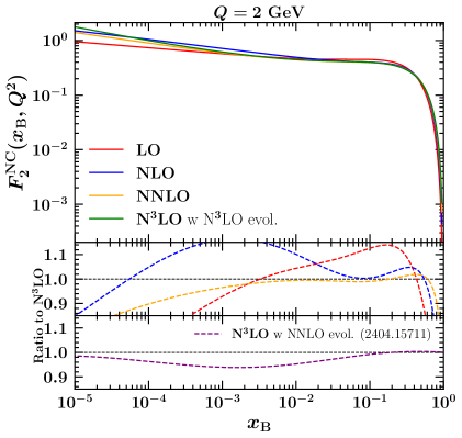
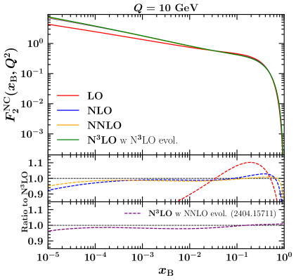
Figure 2: The structure function $F_{2}^{\rm NC}$ plotted as a function of $x_{\rm B}$ in the range $[10^{-5}:0.9]$ at $Q=2$ GeV (left) and $Q=10$ GeV (right). Each plot displays the curves at LO, NLO, NNLO, and N³LO with the middle panel showing the ratio to N³LO. The lowest panel shows the ratio of the N³LO with NNLO evolution to the full N³LO result. Adapted from Ref. Bertone:2024dpm using the full N³LO evolution.

It shows the full charged-lepton neutral current $F_{2}$ structure function ($F_{2}^{\rm NC}$) at various perturbative orders, for two values of $Q$ ($2$ GeV and $10$ GeV). It also shows the relative difference of the various orders with respect to N³LO, and in the lower panel the ratio of the N³LO result of Ref. Bertone:2024dpm to that obtained here with the full evolution. As can be seen by comparing to the original figures and from the lowest panel, the N³LO evolution has the effect at low $Q$ of increasing the N³LO $F_{2}^{\rm NC}$ by a few percent, at least for $x$-values in the range $10^{-4}$ to $10^{-1}$.

4 Evolution including QED contributions

The combined QED+QCD evolution, as implemented in hoppet since version 2.0.0 (and earlier in a dedicated qed branch), was first described in Refs. Manohar:2016nzj , Manohar:2017eqh , Buonocore:2020nai , Buonocore:2021bsf . The determination of which contributions to include follows a consistent approach based on the so-called “phenomenological” counting scheme. Within this scheme, one considers the QED coupling $\alpha$ to be of order $\alpha_{s}^{2}$, and takes the photon (lepton) PDF to be of order $\alpha L$ ($\alpha^{2}L^{2}$), where $L$ is the logarithm of the ratio of the factorisation scale to a typical hadronic scale and is considered to be of order $L\sim 1/\alpha_{s}$. In contrast, quark and gluon PDFs are considered to be of order $(\alpha_{s}L)^{n}={\cal O}(1)$. From this point of view, NNLO (3-loop) QCD evolution provides control of terms of order up to $\alpha_{s}^{n+2}L^{n}\sim\alpha_{s}^{2}$. To achieve a corresponding accuracy when including QED contributions, hoppet has been extended to account for

1. 1-loop QED splitting functions Roth:2004ti , which first contribute at order $\alpha L\sim\alpha_{s}$, i.e. count as NLO QCD corrections;

2. 1-loop QED running coupling, including lepton and quark thresholds, which first contributes at order $\alpha^{2}L^{2}\sim\alpha_{s}^{2}$, i.e. like NNLO QCD;

3. 2-loop mixed QCD-QED splitting functions deFlorian:2015ujt , which first contribute at order $\alpha\alpha_{s}L\sim\alpha_{s}^{2}$, i.e. count as NNLO QCD corrections;

4. optionally, the 2-loop pure QED $P_{\ell q}$ splitting function deFlorian:2016gvk , which brings absolute accuracy $\alpha^{2}L\sim\alpha_{s}^{3}$ to the lepton distribution (which starts at $\alpha^{2}L^{2}\sim\alpha_{s}^{2}$). In an absolute counting of accuracy, this is not needed. However, if one wants lepton distributions to have the same relative NLO accuracy as the photon distribution, it should be included.

The code could be extended systematically to aim at a higher accuracy. For instance, if one wished to reach N³LO accuracy in the phenomenological counting, one would need to include 3-loop mixed QCD-QED splitting functions at order $\alpha\alpha_{s}^{2}$, which contribute at order $\alpha\alpha_{s}^{2}L\sim\alpha_{s}^{3}$ but are currently not available, the full 2-loop pure QED splitting functions deFlorian:2016gvk , and the 2-loop mixed QED-QCD contributions to the running of the QED coupling, which contribute at order $\alpha^{2}\alpha_{s}L^{2}\sim\alpha_{s}^{3}$ (see e.g. Cieri:2018sfk ).

The rest of this section is structured as follows: Section 4.1 gives a technical discussion of the implementation of the QED evolution. Some readers may prefer to skip or skim this on a first reading. Section 4.2 shows how to get QED evolution in the streamlined interface, which is relatively straightforward.

4.1 Implementation of the QED extension

QED coupling

A first ingredient is the setup of the QED coupling object, defined in module qed_coupling:

⬇

type qed_coupling

real(dp) :: m_light_quarks

real(dp) :: mc, mb, mt

integer :: n_thresholds

integer :: nflav(3, 0:n_thresholds) ! first index: 1 = nleptons, 2=ndown, 3=nup

real(dp) :: thresholds(0:n_thresholds+1)

real(dp) :: b0_values(n_thresholds)

real(dp) :: alpha_values(n_thresholds)

end type qed_coupling

This is initialized through a call to

⬇

subroutine InitQEDCoupling(coupling, m_light_quarks, &

& m_heavy_quarks(4:6) [,value_at_scale_0])

type(qed_coupling), intent(out) :: coupling

real(dp), intent(in) :: m_light_quarks, m_heavy_quarks(4:6)

real(dp), optional, intent(in) :: value_at_scale_0 ! defaults to alpha_qed_scale_0

[...]

end subroutine InitQEDCoupling

It initialises the parameters relevant to the QED coupling and its running. The electromagnetic coupling at scale zero is set by default to its PDG Thomson value ParticleDataGroup:2022pth value, unless the optional argument value_at_scale_0 is provided, in which case the latter is taken.

The running is performed at leading order level, using seven thresholds: a common effective mass for the three light quarks (m_light_quarks), the three lepton masses (hard-coded to their 2025 PDG values ParticleDataGroup:2024cfk in the src/qed_coupling.f90 file), and the three masses of the heavy quarks (m_heavy_quarks(4:6)). The common value of the light quark masses is used to mimic the physical evolution in the region $0.1\;\mathrm{GeV}\lesssim\mu\lesssim 1\;\mathrm{GeV}$, which involves hadronic states. Using a value of $0.1055\;\mathrm{GeV}$ generates QED coupling values at the masses of the $\tau$ lepton ($1/133.444$) and $Z$-boson ($1/127.938$) that agree to within relative $\sim 1\times 10^{-4}$ (and $1\sigma$) accuracy with the $\overline{\mathrm{MS}}$ values ($1/(133.450\pm 0.008)$ and $1/(127.930\pm 0.006)$) from the “Electroweak and constraints on New Physics” section of the 2024 Particle Data Group review ParticleDataGroup:2024cfk .

The quark and lepton masses are used to set all thresholds where the fermion content changes. The values of the thresholds are contained in an array threshold(0:8). The threshold(1:7) entries are active thresholds, while threshold(0) is set to zero and threshold(8) to an arbitrary large number (currently $10^{200}$). For a given $Q$, the code identifies the index i such that threshold(i-1)$<Q<$ threshold(i). The flavour content at a given $Q$ is then accessible through the integer array nflav(3,0:n_thresholds), where the nflav(1:3,i) entries indicate respectively the number of leptons, down-type, and up-type quarks at a given $Q$. The nflav(:,:) array is then used to compute the $\beta_{0,\rm QED}$ function b0_values(1:n_thresholds) at the seven threshold values and this is finally used to compute the value of the QED coupling alpha_values(1:n_thresholds) at the threshold values. The function Delete(qed_coupling) is also provided for consistency with general hoppet conventions, although in this case it does nothing. After this initialisation, the function Value(qed_coupling,mu) returns the QED coupling at scale $\mu$.

QED splitting matrices

The QED splitting matrices are stored in the object

⬇

type qed_split_mat

type(qed_split_mat_lo) :: lo

type(qed_split_mat_nlo) :: nlo

type(qed_split_mat_nnlo) :: nnlo

end type qed_split_mat

defined in qed_objects.f90. This contains the LO, NLO and NNLO splitting matrices

⬇

! a leading-order splitting matrix (multiplies alpha/2pi)

type qed_split_mat_lo

type(grid_conv) :: Pqq_01, Pqy_01, Pyq_01, Pyy_01

integer :: nu, nd, nl, nf

end type qed_split_mat_lo

! a NLO splitting matrix (multiplies (alpha alpha_s)/(2pi)^2)

type qed_split_mat_nlo

type(grid_conv) :: Pqy_11, Pyy_11, Pgy_11

type(grid_conv) :: Pqg_11, Pyg_11, Pgg_11

type(grid_conv) :: PqqV_11, PqqbarV_11, Pgq_11, Pyq_11

integer :: nu, nd, nl, nf

end type qed_split_mat_nlo

! a NNLO splitting matrix (multiplies (alpha/(2pi) )^2)

! contains only Plq splitting!

type qed_split_mat_nnlo

type(grid_conv) :: Plq_02

integer :: nu, nd, nl, nf

end type qed_split_mat_nnlo

Above, y denotes a photon and the pairs of integers 01, 11 and 02 denote the orders in the QCD and QED couplings, respectively. Besides the number of quarks nf, these splitting matrices also need the number of up-type (nu) and down-type quarks (nd) separately, and the number of leptons (nl). Note that the splitting functions of order $\alpha$ (i.e. 01) for the leptons are simply obtained from the ones involving quarks by adjusting colour factors and couplings.

A call to the subroutine

⬇

subroutine InitQEDSplitMat(grid, qed_split)

use qed_splitting_functions

type(grid_def), intent(in) :: grid

type(qed_split_mat), intent(inout) :: qed_split

[...]

end subroutine InitQEDSplitMat

initializes the qed_split_mat object qed_split and sets all QED splitting functions on the given grid. The above QED objects can be used for any sensible value of the numbers of flavours, on the condition that one first registers the current number of flavours with a call to

⬇

QEDSplitMatSetNf(qed_split, nl, nd, nu)

where nl, nd and nu are respectively the current numbers of light leptons, down-type and up-type quarks. In practice, this is always handled internally by the QED-QCD evolution routines, based on the thresholds encoded in the QED coupling. The one situation where a user would need to call this routine directly is if they wish to manually carry out convolutions of the QED splitting functions with a PDF.

Subroutines Copy and Delete are also provided for the qed_split_mat type. As in the pure QCD case, convolutions with QED splitting functions can be represented by the .conv. operator or using the product sign *.

PDF arrays with photons and leptons

A call to the subroutine

⬇

subroutine AllocPDFWithPhoton(grid, pdf)

type(grid_def), intent(in) :: grid

real(dp), pointer :: pdf(:,:)

[...]

end subroutine AllocPDFWithPhoton

allocates PDFs (pdf) including photons, while a call to

⬇

subroutine AllocPDFWithLeptons(grid, pdf)

type(grid_def), intent(in) :: grid

real(dp), pointer :: pdf(:,:)

[...]

end subroutine AllocPDFWithLeptons

allocates PDFs including both photons and leptons. The two dimensions of the pdf refer respectively to the index of the $x$ value in the grid, and to the flavour index. The flavour indices for photons and leptons are given by

⬇

integer, parameter, public :: iflv_photon = 8

integer, parameter, public :: iflv_electron = 9

integer, parameter, public :: iflv_muon = 10

integer, parameter, public :: iflv_tau = 11

where each pdf(:,9:11) contains the sum of a lepton and anti-lepton flavour (which are identical). Note that if one were to extend the calculation of lepton PDFs to higher order in $\alpha$, then an asymmetry in the lepton and anti-lepton distribution would arise, due to the Plq_03 splitting function. In fact, at that order, there are also graphs with three electromagnetic vertices on the quark line and three on the lepton line, that change sign if the lepton line is charge-conjugated. In that case it would become useful to have separate indices for leptons and anti-leptons.

The subroutine AllocPDFWithPhotons allocates the pdf array with the flavour index from -6 to 8, while in the subroutine AllocPDFWithLeptons, the flavour index extends from -6 to 11.

PDF tables with photons and leptons

Next one needs to prepare a pdf_table object forming the interpolating grid for the evolved PDF’s. We recall that the pdf_table object contains an underlying array pdf_table%tab(:,:,:), where the first index loops over $x$ values, the second loops over flavours and the last loops over $Q^{2}$ values.

This is initialized by a call to

⬇

subroutine AllocPdfTableWithLeptons(grid, pdftable, Qmin, Qmax &

& [, dlnlnQ] [, lnlnQ_order] [, freeze_at_Qmin])

use qed_objects

type(grid_def), intent(in) :: grid

type(pdf_table), intent(inout) :: pdftable

real(dp), intent(in) :: Qmin, Qmax

real(dp), intent(in), optional :: dlnlnQ

integer, intent(in), optional :: lnlnQ_order

logical, intent(in), optional :: freeze_at_Qmin

[...]

end subroutine AllocPdfTableWithLeptons

that is identical to the one without photon or leptons, the only difference is that the maximum pdf flavour index in pdf_table%tab now includes the photon and leptons. An analogous subroutine AllocPdfTableWithPhoton includes the photon but no leptons.

Evolution with photons and leptons

To fill a table via an evolution from an initial scale, one calls the subroutine

⬇

subroutine EvolvePdfTableQED(table, Q0, pdf0, dh, qed_split, &

& coupling, coupling_qed, nloop_qcd, nloopqcd_qed, with_Plq_nnloqed)

type(pdf_table), intent(inout) :: table

real(dp), intent(in) :: Q0

real(dp), intent(in) :: pdf0(:,:)

type(dglap_holder), intent(in) :: dh

type(qed_split_mat), intent(in) :: qed_split

type(running_coupling), intent(in) :: coupling

type(qed_coupling), intent(in) :: coupling_qed

integer, intent(in) :: nloop_qcd, nloopqcd_qed

logical, optional, intent(in) :: with_Plq_nnloqed

[...]

end subroutine EvolvePdfTableQED

where table is the output, Q0 the initial scale and pdf0 is the PDF at the initial scale. We recall that the lower and upper limits on scales in the table are as set at initialisation time for the table. When nloopqcd_qed is set to 1 (0) mixed QCD-QED effects are (are not) included in the evolution. Setting the variable with_Plq_nnloqed=.true. includes also the NNLO $P_{lq}$ splittings in the evolution.

To perform the evolution EvolvePdfTableQED calls the routine

⬇

subroutine QEDQCDEvolvePDF(dh, qed_sm, pdf, coupling_qcd, coupling_qed,&

& Q_init, Q_end, nloop_qcd, nqcdloop_qed, with_Plq_nnloqed)

type(dglap_holder), intent(in), target :: dh

type(qed_split_mat), intent(in), target :: qed_sm

type(running_coupling), intent(in), target :: coupling_qcd

type(qed_coupling), intent(in), target :: coupling_qed

real(dp), intent(inout) :: pdf(0:,ncompmin:)

real(dp), intent(in) :: Q_init, Q_end

integer, intent(in) :: nloop_qcd

integer, intent(in) :: nqcdloop_qed

logical, optional, intent(in) :: with_Plq_nnloqed

[...]

end subroutine QEDQCDEvolvePDF

Given the pdf at an initial scale Q_init, it evolves it to scale Q_end, overwriting the pdf array. In order to get interpolated PDF values from the table we use the EvalPdfTable_* calls, described in Section 7.2 of Ref. Salam:2008qg . However the pdf array that is passed as an argument and that is set by those subroutines should range not from (-6:6) but instead from (-6:8) if the PDF just has photons and (-6:11) if the PDF also includes leptons.

Note that at the moment, when QED effects are included, cached evolution is not supported.

4.2 Streamlined interface with QED effects

The streamlined interface including QED effects works as in the case of pure QCD evolution. One has to add the following call

⬇

logical use_qed, use_qcd_qed, use_Plq_nnlo

...

call hoppetSetQED(use_qed, use_qcd_qed, use_Plq_nnlo)

before using the streamlined interface routines. The use_qed argument turns QED evolution on/off at order ${\cal O}(\alpha)$ (i.e. items 1 and 2 in the enumerated list at the beginning of Sec. 4). The use_qcd_qed one turns mixed QCD$\times$QED effects on/off in the evolution (i.e. item 3) and use_Plq_nnlo turns the order $\alpha^{2}P_{\ell q}$ splitting function on/off (i.e. item 4). Without this call, all QED corrections are off.

With the above, the streamlined interface can then be used as normal. E.g. by calling the hoppetEvolve(...) function to fill the PDF table and hoppetEval(x,Q,f) to evaluate the PDF at a given $x$ and $Q$. Note that the f array in the latter call must be suitably large, e.g. f(-6:11) for a PDF with leptons. Examples of the streamlined interface being used with QED evolution can be found in

example_f90/tabulation_example_qed_streamlined.f90
example_cpp/tabulation_example_qed.cc

5 Python interface

From version 2.0.0, hoppet also includes a Python interface to the most common evolution routines. It currently includes exactly the same functionality as the streamlined interface, and can be called in much the same way. The names of functions and routines are the same as in the streamlined interface, but stripped of the hoppet prefix. The interface can be obtained from PyPi by invoking

⬇

pip install hoppet

Alternatively the interface can be built by CMake with -DHOPPET_BUILD_PYINTERFACE=ON (cf. Section 6 for details on building with CMake). In both cases the interface can be imported into a Python instance through import hoppet. For a simple tabulation example, the user should take a look at example_py/tabulation_example.py (and in the same directory for a number of other illustrative examples of how to use the interface, including in conjunction with LHAPDF LHAPDF ). The interface uses SWIG (Simplified Wrapper and Interface Generator) which therefore needs to be available on the system if building with CMake. It can be installed through most package managers (e.g. apt install swig, brew install swig) but can also be obtained from the SWIG GitHub repository.

One significant difference between the Python interface and the streamlined interface is that Python does not provide native support for pointers. A number of C++ routines fill an array of PDF flavours that is passed as a pointer argument. Instead in Python, those routines return a Python list directly. For instance, where in C++ one might have the call

⬇

#include "hoppet.h"

[...]

double x = ...;

double Q = ...;

double pdf[13];

[...]

hoppetEval(x, Q, pdf);

instead in Python one would have

⬇

import hoppet as hp

[...]

x = ...

Q = ...

pdf = hp.Eval(x,Q)

This is relevant not just for evaluation of PDFs, but also in setting initial conditions. For example the Assign, CachedEvolve, and Evolve routines should be passed a function of x and Q that returns an object that corresponds to array of flavours (it can be a numpy Harris:2020xlr array of a Python list; see the hera_lhc(x,Q) function in tabulation_example.py for an explicit example).

In addition to the examples provided in example_py/ we have also developed a small tool that loads a grid from LHAPDF at an initial scale and evolves it with hoppet over a large range of $Q$. The resulting grids are then compared between hoppet and LHAPDF to determine the relative accuracy of the LHAPDF grids. The tool, along with some documentation, can be found at https://github.com/hoppet-code/hoppet-lhapdf-grid-checker.

6 CMake build system

In v1.x, hoppet used a hand-crafted ./configure script followed by make [install]. As of v2 hoppet uses CMake.

For a typical user it will be enough to invoke the following lines from the main directory

⬇

cmake -S . -B build

cmake --build build -j

ctest --test-dir build [-j8]

cmake --install build

This will compile and install hoppet, along with the streamlined interface. Note that make install will typically install in a location that requires root privileges, unless a user has specified a custom prefix (through -DCMAKE_INSTALL_PREFIX=/install/path). A number of options can be passed to CMake. They are documented in CMakeLists.txt and can be printed on screen by a call to cmake -LH .. from the build directory.

Of particular note to most users are

⬇

option(HOPPET_USE_EXACT_COEF "Use exact coefficient functions" OFF)

option(HOPPET_BUILD_EXAMPLES "Build examples" ON)

option(HOPPET_ENABLE_TESTING "Enable testing. Requires building the examples." ON)

option(HOPPET_BUILD_BENCHMARK "Build benchmark." ON)

option(HOPPET_BUILD_PYINTERFACE "Build python interface." OFF)

option(HOPPET_ENABLE_FPES "Enable trapping for the floating point exceptions." OFF)

option(HOPPET_BUILD_TESTDIR "Enable build of the code in the test directory." OFF)

They can be set in the usual cmake way, e.g.

⬇

cmake -S . -B build -DHOPPET_USE_EXACT_COEF=ON

to compile hoppet with the exact coefficient functions. Note that the Python interface is not compiled by default, because we anticipate that users of Python will prefer to obtain hoppet through pip install hoppet.

7 Saving LHAPDF grids

A minor new feature of this release is the possibility to save a hoppet table in the form of an LHAPDF6 LHAPDF grid. The main routine has the following structure

⬇

subroutine WriteLHAPDFFromPdfTable(table, coupling, basename, pdf_index, &

& iy_increment, flav_indices, flav_pdg_ids, flav_rescale)

use qed_objects

type(pdf_table), intent(in) :: table

type(running_coupling), intent(in) :: coupling

character(len=*), intent(in) :: basename

integer, intent(in) :: pdf_index

integer, optional, intent(in) :: iy_increment

integer, optional, intent(in) :: flav_indices(:), flav_pdg_ids(:)

real(dp), optional, intent(in) :: flav_rescale(:)

A user has to provide a table and associated coupling object along with a string basename and the pdf_index as needed by LHAPDF. If pdf_index is equal to 0 then the routine outputs the contents of the table in basename_0000.dat and writes a template basename.info again in LHAPDF format. hoppet fills most of the entries in the .info file, but a few need to be edited manually by the user. For any other value of pdf_index, only the corresponding .dat file gets written.

By default, the code uses the same grid spacing as in the internal hoppet table (iy_increment = 1) and prints all the possible flavours of the PDF, even if they are zero. The user can overwrite this default behaviour by providing an array of flavours and their pdg values. If iy_increment > 1 a coarser grid is provided by skipping over iy_increment - 1 points in the grid. The flav_rescale is currently needed for the lepton PDF which is provided as the sum over flavour and anti-flavour and therefore needs an extra factor half. The flav_rescale array only needs to be provided if the user is also providing the array of flavours and pdf values.

Finally the routine can also be accessed from the streamlined interface for C++ or Python usage. In this case the routine is significantly simplified and only takes basename and the pdf_index arguments, for instance in C++ like this

⬇

#include "hoppet.h"

#include <string>

...

int main () {

...

const std::string basename = ...;

const int pdf_index = ...;

hoppetWriteLHAPDFGrid(basename, pdf_index);

...

}

The routine writes the contents of the streamlined interface tables(0) and hence requires that this object has been filled either through a call to hoppetAssign or hoppetEvolve.

8 Updated performance studies

In this section we present some updated performance studies relative to Section 9 of Ref. Salam:2008qg , mainly reflecting updated hardware and compilers of 2025, but also the standard nested grid choice that is obtained with the streamlined interface or, from the modern Fortran interface by calling InitGridDefDefault(grid, dy, ymax[, order]), with the default choice of interpolation order=-6. The InitGridDefDefault(...) routine is new relative to v1 and sets up the following grid

⬇

call InitGridDef(gdarray(4),dy/27.0_dp, 0.2_dp, order)

call InitGridDef(gdarray(3),dy/9.0_dp, 0.5_dp, order)

call InitGridDef(gdarray(2),dy/3.0_dp, 2.0_dp, order)

call InitGridDef(gdarray(1),dy, ymax , order)

call InitGridDef(grid,gdarray(1:4),locked=.true.)

Users will usually only need a different choice if they plan studies at $x$ very close to $1$ or if they wish to explore fine optimisation of grid choices.

We split our study here into two parts: the accuracy of PDF evolution and tabulation (section 8.1) and PDF evaluation (section 8.2). The latter also outlines new functionality for choosing interpolation orders differently in the PDF evaluation versus the PDF evolution and it includes comparisons to LHAPDF.

8.1 PDF evolution and tabulation

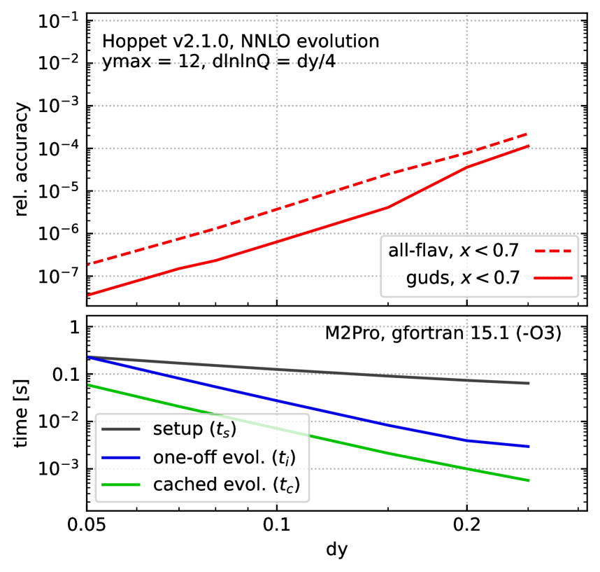
(a)

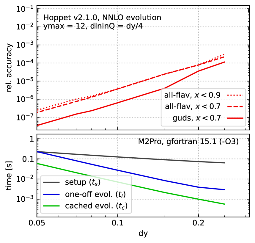
(b)

Figure 3: Accuracy (top) and timing (bottom) versus dy at (a) NNLO and (b) N³LO in hoppet v2.1.0. The accuracy corresponds to the worst fractional accuracy for any flavour, at any $x$ value below the corresponding limit, as described in the text. The timings were obtained on an M2Pro with gfortran v15.1 and -O3 optimisation. We have further used ymax = 12 and dlnlnQ = dy/4.

The studies are performed using the initial condition of Ref. Dittmar:2005ed as detailed in Section 9.1 of Ref. Salam:2008qg , evolved in the VFNS scheme. At NNLO we use the parametrised splitting functions and mass thresholds, as per hoppet defaults. To assess the accuracy we first create a reference run with a very high density grid. We then run hoppet with different values of grid spacing dy, keeping dlnlnQ = dy/4. The accuracy is then computed by looking at the largest relative deviation from the reference run across either all flavours (all-flav) or the light flavours (guds). The full tabulation covers the range $10^{-5}<x<1$, $2<Q<10^{4}\,\text{GeV}$. At $x$ values close to $1$, the numerical precision degrades because the parton distribution functions become a very steep function of $\ln x$. However, the parton distributions have small values there and so we carry out our precision study with two potential upper limits on the $x$ value being probed, $x<0.9$ and $x<0.7$. We also exclude PDF flavours in the $x$ and $Q$ vicinity of any sign change, as per Ref. Salam:2008qg .

The results for the accuracy study can be seen in the top panels of Figures 3(a)–3(b) at NNLO and N³LO respectively, as a function of dy. At NNLO, the accuracy comes out similar to previous versions of hoppet. With dy = 0.2 one obtains a relative accuracy of $10^{-4}$ across all flavours in the range $x<0.9$. At the finest grid spacing dy = 0.05, a relative accuracy of few times $10^{-7}$ can be achieved, good enough for precise benchmark comparisons as were for instance carried out in Refs. Dittmar:2005ed , Bertone:2024dpm . For comparison, the recent benchmark of aN³LO codes in Ref. Cooper-Sarkar:2024crx reaches a relative precision of a few times $10^{-4}$ at best (cf. the gluon PDF at $x=10^{-2}$ in Table 2 and Table 1 of Ref. Cooper-Sarkar:2024crx which differ by $\sim 8\cdot 10^{-4}$.)

The scaling of the precision is roughly consistent with a power law in dy. In particular the Runge-Kutta algorithm for the $Q^{2}$ evolution is expected to yield an error proportional to $\texttt{dlnlnQ}^{4}$, which, given our choice of $\texttt{dlnlnQ}=\texttt{dy}/4$ translates into a behaviour $\sim\texttt{dy}^{4}$ in Fig. 3. The observed scaling is, if anything, slightly better than this, given the factor of $1000$ improvement in accuracy when reducing dy by a factor of $5$ from $0.2$ to $0.04$. The precise scaling depends on whether it is Runge-Kutta or the splitting function grid representation that dominates the error. At N³LO we observe a similar level of accuracy as at NNLO, except for a slight worsening associated with the heavy-flavour components.

For the timing studies we again run hoppet for different values of dy, on an M2Pro (MacOS 15.6.1) with gfortran v15.1 and -O3 optimisation. As discussed in Salam:2008qg , the time spent in hoppet for a given analysis can be expressed as follows, depending on whether or not one carries out cached evolution (pre-evolution):

$$t_{\text{no pre-ev}} =t_{s}+n_{\alpha}t_{\alpha}+n_{i}(t_{i}+n_{xQ}\,t_{xQ})\,,$$ (1a)

$$t_{\text{with pre-ev}} =t_{s}+n_{\alpha}(t_{\alpha}+t_{p})+n_{i}(t_{c}+n_{xQ}\,t_{xQ})\,,$$ (1b)

where $t_{s}$ is the time for setting up the splitting functions and mass threshold functions, $n_{\alpha}$ is the number of different running couplings that one has, $t_{\alpha}$ is the time for initialising the coupling, $n_{i}$ is the number of PDF initial conditions that one wishes to consider, $t_{i}$ is the time to carry out the tabulation and evolution for a single initial condition, $n_{xQ}$ is the number of points in $x,Q$ at which one evaluates the full set of flavours once per PDF initial condition; in the case with cached evolution, $t_{p}$ is the time for preparing a cached evolution and $t_{c}$ is the time for performing the cached evolution. Finally, $t_{xQ}$ is the time it takes to evaluate the PDFs at a given value of $(x,Q)$ once the tabulation has been performed.

Here we focus on $t_{s}$, $t_{i}$, and $t_{c}$. The results can be seen in the bottom panels of Figures 3(a)–3(b) at NNLO and N³LO respectively. The expected scaling is $t_{i},t_{c}\sim(\text{{dy}}^{2}\text{{dlnlnQ}})^{-1}$, which for our choice of $\texttt{dlnlnQ}\propto\texttt{dy}$ reduces to $1/\text{{dy}}^{3}$. That is consistent with what is seen in the plot. Turning to the setup time, at NNLO $t_{s}\sim 60-300\,\mathrm{ms}$ dominates over the evolution time across almost all dy values that we study. It scales slightly more slowly than $t_{s}\sim 1/\texttt{dy}$.

We note that when using cached evolution, the evolution time $t_{c}$ reaches as little as $1\,\mathrm{ms}$ for dy = 0.2. Comparing these numbers to those of Table 2 of Ref. Salam:2008qg , which were obtained with 2008 hardware and compilers, we see a speed-up of roughly a factor 10, which we attribute mainly to improvements in the hardware.

At N³LO evolution times ($t_{i}$ and $t_{c}$) are essentially identical to the NNLO case: for $t_{i}$ the only extra operation that is needed is the addition of the N³LO splitting function to the lower-order ones and at each $Q$ value, this involves ${\cal O}\left(N\right)$ operations for a $y$-grid of size $N$, while the convolution itself involves ${\cal O}\left(N^{2}\right)$ operations. For the cached evolution, there is no additional penalty, because the N³LO contributions are already included in the cached evolution operators. The initialisation times are somewhat larger, in a range from 250 ms to 1 s. The longer time is associated both with the approximate N³LO splitting functions and the mass threshold functions of Ref. BlumleinCode , using the n3lo_nfthreshold_libOME option. In practice the initialisation time remains adequate for most interactive work. In any long-running application where hoppet either has to evolve or access the evolved tables many times, the initialisation time is insignificant.

8.2 Fast PDF access

Here we detail updates for faster PDF access within the modern Fortran and streamlined interfaces (including the Python interface). In earlier versions of hoppet, the interpolation was carried out by a single routine that could flexibly handle any choice of $y$ and $Q$ interpolation orders up to some hard-coded maximum. As of v2.0.0, a number of interpolation-order choices now have dedicated code, which makes it easier for the compiler to optimise the underlying assembly, e.g. with loop unrolling, giving speed gains of almost a factor of three. Additionally new functionality allows the user to modify the interpolation order of the hoppet grids, trading accuracy versus speed.

Specificaly, the user can now globally override any table-specific interpolation order settings by calling one of

⬇

call hoppetSetYLnlnQInterpOrders(yorder, lnlnQorder) ! streamlined interface

or

⬇

call PdfTableOverrideInterpOrders(yorder, lnlnQorder) ! F90 interface

A value of $\texttt{order}=2$ corresponds to quadratic interpolation, $3$ to cubic interpolation, etc. The default interpolation order is quartic in the lnlnQ direction, and |grid%order|-1 in the y direction (bounded to be between 3 and 9 if outside that range). These rather high interpolation orders help ensure good accuracy in a normal hoppet run even with dy=0.2, but come with a speed penalty because of the larger number of operations. However, if PDF evaluation represents a significant fraction of the time for a user’s code, the user can choose to lower the interpolation order and still retain good accuracy by reducing dy and dlnlnQ.

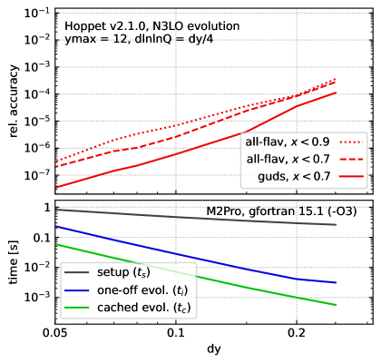
Figure 4: Study of the impact of the choice of the $y$ and $Q$ interpolation orders (oY, oQ) on accuracy (upper panel) and speed (lower panel) for evaluating the PDF table at a given $y$ and $Q$ point. Note that the interpolation order that enters the splitting functions remains $6$ as in Fig. 3. The timing corresponds to the EvalPdfTable_yQ(table,y,Q,vals) modern Fortran call. The timings have been obtained on an M2Pro with gfortran v15.1 and -O3 optimisation. Calling EvalPdfTable_xQ(table,x,Q,vals), or the corresponding functions in the streamlined interfaces, adds about $5\;\mathrm{ns}$. We have further used ymax = 12 and dlnlnQ = dy/4. Note that our accuracy definition is to show the worst accuracy across any $[guds]$ flavour and $x$ value in range. In practice, most points have a significantly higher accuracy. We also show results obtained by interpolating our grids with LHAPDF 6.5.5, calling it from its native C++ interface to maximise its speed.

Fig. 4 shows the accuracy and timing as a function of dy for different interpolation order choices. It compares evolution as in Fig. 3, followed by interpolation with a given order. It illustrates the significant loss in accuracy when decreasing the interpolation order below $4$. For orders of $4$ or higher, the limitation on accuracy is, however, no longer just the interpolation order during PDF evaluation, but also the orders that appear in the grid representation of the splitting functions and of the $Q$ evolution when producing the original table. The time that is shown in the lower panel corresponds to the evaluation of all flavours in one go, via the EvalPdfTable_yQ(...) routine. It ranges from $60\;\mathrm{ns}$ to $100\;\mathrm{ns}$ in going from the $(2,2)$ order combination to $(5,4)$. It is largely independent of dy. Calls to evaluate a single flavour are only $2.5{-}3$ times faster, because of overheads associated with identifying the grid location and calculation interpolation coefficients, which are independent of the number of flavours one evaluates.

Fig. 4 also shows results with LHAPDF, calling it from its native C++ to maximise its speed. We generate an LHAPDF grid for our standard benchmark initial conditions, with a given dy spacing, cf. Section 7, and then examine the difference between the LHAPDF evaluation and our high-accuracy reference. The upper panel of Fig. 4 shows the accuracy with the same definition as used in our other performance results, i.e. the worst relative accuracy observed anywhere for $x<0.7$, across any of the g,u,d,s flavours, as in the solid lines of Fig. 3. For most flavours and most of the $x$ region, the accuracy is better than shown. Interestingly, the LHAPDF accuracy is comparable to hoppet’s quadratic interpolation. At first sight this might be surprising given that LHAPDF uses cubic interpolation: however it is our understanding that in the $x$ direction it uses a cubic spline. The spline effectively sacrifices one of the orders of accuracy in function evaluation and instead uses it to ensure exact continuity of the first derivative. In contrast, hoppet does not enforce continuity of the derivatives but relies on the fact that for high interpolation order any discontinuity of the derivatives will scale as a high power of the grid spacing. Which choice is better may depend on the application. Concerning speed, we find that LHAPDF is somewhere in between our $(4,4)$ and $(5,4)$ choices.

For use-cases where PDF evaluation speed is critical, one option is to read in a PDF grid with LHAPDF, evaluate it at all hoppet grid points and then use hoppet for the interpolation, using a fine grid spacing and a $(2,2)$ interpolation choice. We provide examples for how to do this in Fortran, C++, and Python:

• example_f90/with-lhapdf/lhapdf_to_hoppet.f90: it uses the module hoppet_lhapdf and the associated subroutine LoadLHAPDF(name, imem). The module is in the same directory and can be copied over to a user’s application;

• example_f90/with-lhapdf/lhapdf_to_hoppet_allmembers.f90, same as above but the example shows how to read in and efficiently evaluate all LHAPDF members, with an illustration for computing the PDF uncertainty;

• example_cpp/with-lhapdf/lhapdf_to_hoppet.cc, which includes a routine called void load_lhapdf_assign_hoppet(const string & pdfname, int imem=0) which can be included directly in a user’s application;

• example_py/lhapdf_to_hoppet.py, makes use of hoppet.lhapdf.load(), accessible using “from hoppet import lhapdf”.

The PDF can then be evaluated in the usual way through a call to hoppetEval and likewise for the coupling through hoppetAlphaS. All three examples also print the timings to the screen so that users can check speed on their hardware. Note that these examples are not fully general, and caution should be exercised when using them. Users with more advanced requirements are invited to contact the hoppet authors for assistance.

yorder	lnlnQorder	Time per hoppetEval or LHAPDF xfxQ/EvolvePDF call (ns)
		Fortran	C++	Python
5	4	108	108	295
4	4	92	93	278
3	3	76	77	258
2	2	63	63	244
HOPPET 1.2.0		313	313	–
LHAPDF 6.5.5		520	87	1645
LHAPDF 6.5.5 + patch		114	87	1028

Table 3: Time for a call to hoppetEval, which evaluates all flavours at a given $x,Q$ point. The rows show the timings with different interpolation orders. The results have been obtained with the PDF4LHC21_40 set, on an M2Pro with gfortran-15.1, Apple clang version 17.0.0, O3 optimisation and Python 3.12.7. The hoppet grid spacings are $\texttt{dy}=0.05$ and $\texttt{dlnlnQ}=\texttt{dy}/4$, with $\texttt{ymax}=14$. The table also shows the timings for the equivalent calls in LHAPDF 6.5.5. Version 6.5.5 of LHAPDF, in its Fortran (EvolvePDF(...), lhapdf_xfxq(...)) and Python (pdf.xfxQ(...)) interfaces, loops over an underlying call to single-flavour evaluation (double PDF::xfxQ(int id, double x, double q))), which is why it is significantly slower than the C++ interface, which evaluates all flavours in one go. A proposed patch for the Fortran and Python interfaces has been submitted to LHAPDF with corresponding timings also indicated.

Table 3 illustrates those timings for a range of interpolation orders and across interfaces in different languages. These tests have been carried out with the PDF4LHC21_40 set. Again, they confirm that hoppet with lower interpolation orders can offer a speed gain relative to LHAPDF. That speed gain is moderate in C++, more significant in Fortran and Python. As concerns Fortran, there are straightforward modifications to LHAPDF that would improve its speed and these have been proposed to the LHAPDF authors.

The PDF and $\alpha_{s}$ evaluation routines in hoppet are thread safe. Other parts of the code, notably initialisation and evolution, are not.

9 Conclusion

Version 2 of hoppet brings major additions to its functionality. These include evolution up to N³LO, massless structure function evaluation, QED evolution, a Python interface, a modern build system, functionality for writing LHAPDF grids and significant speed improvements in the interpolation of its internal PDF tables.

Overall hoppet remains highly competitive in terms of speed and accuracy. For example, repeated filling of a full PDF tabulation takes about a millisecond per initial condition, with a relative accuracy of $10^{-4}$ or better for $10^{-5}<x<0.9$. It offers explicit handles to control the accuracy, allowing users to verify the precision of their results and choose the optimal trade-off between speed and precision. Its modern Fortran interface also offers powerful and flexible access to a range of common PDF manipulations such as convolutions with arbitrary splitting and coefficient functions, features that are useful in a variety of contexts.

We hope that this release of hoppet can help provide solid foundations for a range of groups to contribute to the ongoing discussions McGowan:2022nag , NNPDF:2024nan , Cooper-Sarkar:2024crx , Cridge:2024icl , Cooper-Sarkar:2025sqw in the field concerning the impact of N³LO and QED effects in PDF fits. We also hope that the interfaces across computing languages will facilitate the practical aspects of integration with a range of other tools.

Appendix A Perturbative evolution in QCD

First of all we set up the notation and conventions that are used throughout hoppet. The DGLAP equation for a non-singlet parton distribution reads

$$\frac{\partial q(x,Q^{2})}{\partial\ln Q^{2}}=\frac{\alpha_{s}\left(Q^{2}\right)}{2\pi}\int_{x}^{1}\frac{dz}{z}P(z,\alpha_{s}\left(Q^{2}\right))q\left(\frac{x}{z},Q^{2}\right)\equiv\frac{\alpha_{s}\left(Q^{2}\right)}{2\pi}P(x,\alpha_{s}\left(Q^{2}\right))\otimes q\left(x,Q^{2}\right)\ .$$ (2)

The related variable $t\equiv\ln Q^{2}$ is also used in various places in hoppet. The splitting functions in eq. (2) are known exactly up to NNLO in the unpolarised case Furmanski:1980cm , Curci:1980uw , NNLO-NS , NNLO-singlet , and approximately at N³LO Gracey:1994nn , Davies:2016jie , Moch:2017uml , Gehrmann:2023cqm , Falcioni:2023tzp , Gehrmann:2023iah , McGowan:2022nag , NNPDF:2024nan , Moch:2021qrk , Falcioni:2023luc , Falcioni:2023vqq , Moch:2023tdj , Falcioni:2024xyt , Falcioni:2024qpd :

$$P(z,\alpha_{s}\left(Q^{2}\right))=P^{(0)}(z)+\frac{\alpha_{s}\left(Q^{2}\right)}{2\pi}P^{(1)}(z)+\left(\frac{\alpha_{s}\left(Q^{2}\right)}{2\pi}\right)^{2}P^{(2)}(z)+\left(\frac{\alpha_{s}\left(Q^{2}\right)}{2\pi}\right)^{3}P^{(3)}(z)\ ,$$ (3)

and up to NNLO Mertig:1995ny , Vogelsang:1996im , Moch:2014sna , Moch:2015usa , Blumlein:2021enk , Blumlein:2021ryt in the polarised case. The generalisation to the singlet case is straightforward, as it is to the case of time-like evolution, relevant for example for fragmentation function analysis, where NNLO results are also available Mitov:2006ic , Moch:2007tx , Almasy:2011eq .

As with the splitting functions, all perturbative quantities in hoppet are defined to be coefficients of powers of $\alpha_{s}/2\pi$. The one exception is the $\beta$-function coefficients of the running coupling equation:

$$\frac{d\alpha_{s}}{d\ln Q^{2}}=\beta\left(\alpha_{s}\left(Q^{2}\right)\right)=-\alpha_{s}(\beta_{0}\alpha_{s}+\beta_{1}\alpha_{s}^{2}+\beta_{2}\alpha_{s}^{3}+\beta_{3}\alpha_{s}^{4})\ .$$ (4)

The evolution of the strong coupling and the parton distributions can be performed in both the fixed flavour-number scheme (FFNS) and the variable flavour-number scheme (VFNS). In the VFNS case we need the matching conditions between the effective theories with $n_{f}$ and $n_{f}+1$ light flavours for both the strong coupling $\alpha_{s}\left(Q^{2}\right)$ and the parton distributions at the heavy quark mass threshold $m_{h}^{2}$.

These matching conditions for the parton distributions receive non-trivial contributions at higher orders. In the $\overline{\mathrm{MS}}$ (factorisation) scheme, for example, carrying out the matching at a scale equal to the heavy-quark mass, these begin at NNLO: for light quarks $q_{l,i}$ of flavour $i$ (quarks that are considered massless below the heavy quark mass threshold $m_{h}^{2}$) the matching between their values in the $n_{f}$ and $n_{f}+1$ effective theories reads:

$$q_{l,i}^{\,(n_{f}+1)}(x,m_{h}^{2})+q_{l,-i}^{\,(n_{f}+1)}(x,m_{h}^{2}) =q_{l,i}^{\,(n_{f})}(x,m_{h}^{2})+q_{l,-i}^{\,(n_{f})}(x,m_{h}^{2})$$

$$+A^{\rm NS,+}_{qq,h}(x)\otimes\left(q_{l,i}^{\,(n_{f})}(x,m_{h}^{2})+q_{l,-i}^{\,(n_{f})}(x,m_{h}^{2})\right)$$

$$+\frac{1}{n_{f}}\Big\{A^{\rm PS}_{qq,h}(x)\otimes\Sigma^{\,(n_{f})}(x,m_{h}^{2})$$

$$+A^{\rm S}_{qg,h}(x)\otimes g^{\,(n_{f})}(x,m_{h}^{2})\Big\}\ ,$$

$$q_{l,i}^{\,(n_{f}+1)}(x,m_{h}^{2})-q_{l,-i}^{\,(n_{f}+1)}(x,m_{h}^{2}) =q_{l,i}^{\,(n_{f})}(x,m_{h}^{2})-q_{l,-i}^{\,(n_{f})}(x,m_{h}^{2})$$

$$+A^{\rm NS,-}_{qq,h}(x)\otimes\left(q_{l,i}^{\,(n_{f})}(x,m_{h}^{2})-q_{l,-i}^{\,(n_{f})}(x,m_{h}^{2})\right)\ ,$$ (5)

where $i=1,\ldots n_{f}$, while for the gluon distribution, the heavy quark PDF $q_{h}$, and the singlet PDF $\Sigma(x,Q^{2})$ (defined in Table 4) one has :

$$g^{(n_{f}+1)}(x,m_{h}^{2}) =g^{\,(n_{f})}(x,m_{h}^{2})+A_{\rm gq,h}^{\rm S}(x)\otimes\Sigma^{(n_{f})}(x,m_{h}^{2})+A_{\rm gg,h}^{\rm S}(x)\otimes g^{(n_{f})}(x,m_{h}^{2})\ ,$$

$$(q_{h}+\bar{q}_{h})^{(n_{f}+1)}(x,m_{h}^{2}) =A_{\rm hq}^{\rm S}(x)\otimes\Sigma^{(n_{f})}(x,m_{h}^{2})+A_{\rm hg}^{\rm S}(x)\otimes g^{(n_{f})}(x,m_{h}^{2})\ ,$$

$$\Sigma^{(n_{f}+1)}(x,m_{h}^{2}) =\Sigma^{\,(n_{f})}(x,m_{h}^{2})+\left[A^{\rm NS,+}_{qq,h}(x)+A^{\rm PS}_{qq,h}(x)+A_{\rm hq}^{\rm S}(x)\right]\otimes\Sigma^{(n_{f})}(x,m_{h}^{2})$$

$$+\left[A^{\rm S}_{qg,h}(x)+A_{\rm hg}^{\rm S}(x)\right]\otimes g^{(n_{f})}(x,m_{h}^{2})$$ (6)

with $q_{h}=\bar{q}_{h}$. Up to N³LO the matching coefficients have the following expansions in $\alpha_{s}$

$$A^{\rm NS,\pm}_{qq,h}(x) =\left(\frac{\alpha_{s}(m_{h}^{2})}{2\pi}\right)^{2}A^{\rm NS,\pm,(2)}_{qq,h}(x)+\left(\frac{\alpha_{s}(m_{h}^{2})}{2\pi}\right)^{3}A^{\rm NS,\pm,(3)}_{qq,h}(x)\ ,$$

$$A^{\rm S}_{gk,h}(x) =\left(\frac{\alpha_{s}(m_{h}^{2})}{2\pi}\right)^{2}A^{\rm S,(2)}_{gk,h}(x)+\left(\frac{\alpha_{s}(m_{h}^{2})}{2\pi}\right)^{3}A^{\rm S,(3)}_{gk,h}(x),\quad k=q,g\ ,$$

$$A^{\rm S}_{hk}(x) =\left(\frac{\alpha_{s}(m_{h}^{2})}{2\pi}\right)^{2}A^{\rm S,(2)}_{hk}(x)+\left(\frac{\alpha_{s}(m_{h}^{2})}{2\pi}\right)^{3}A^{\rm S,(3)}_{hk}(x),\quad k=q,g\ ,$$

$$A^{\rm PS}_{qq,h}(x) =\left(\frac{\alpha_{s}(m_{h}^{2})}{2\pi}\right)^{3}A^{\rm PS,(3)}_{qq,h}(x)\,,$$

$$A^{\rm S}_{qg,h}(x) =\left(\frac{\alpha_{s}(m_{h}^{2})}{2\pi}\right)^{3}A^{\rm S,(3)}_{qg,h}(x)\,.$$ (7)

At $\mathcal{O}(\alpha_{S}^{2})$ we have that $A^{\rm NS,+}_{qq,h}(x)=A^{\rm NS,-}_{qq,h}(x)$ whereas they start to differ at $\mathcal{O}(\alpha_{S}^{3})$. The NNLO matching coefficients were computed in NNLO-MTM and the N³LO matching coefficients in Bierenbaum:2009mv , Ablinger:2010ty , Kawamura:2012cr , Blumlein:2012vq , ABLINGER2014263 , Ablinger:2014nga , Ablinger:2014vwa , Behring:2014eya , Ablinger:2019etw , Behring:2021asx , Fael:2022miw , Ablinger:2023ahe , Ablinger:2024xtt , BlumleinCode . Notice that the above conditions will lead to small discontinuities of the PDFs in its evolution in $Q^{2}$, which are cancelled by similar matching terms in the coefficient functions in massive VFN schemes, resulting in continuous physical observables. In particular, the heavy-quark PDFs start from a non-zero value at threshold at NNLO, which sometimes can even be negative.

The corresponding N³LO relation for the matching of the $\overline{\mathrm{MS}}$ coupling constant at the heavy quark threshold $m^{2}_{h}$ is given by

$$\alpha_{s}^{\,(n_{f}+1)}(m_{h}^{2})\>=\>\alpha_{s}^{\,(n_{f})}(m_{h}^{2})+C_{2}\left(\frac{\alpha_{s}^{\,(n_{f})}(m_{h}^{2})}{2\pi}\right)^{3}+C_{3}\left(\frac{\alpha_{s}^{\,(n_{f})}(m_{h}^{2})}{2\pi}\right)^{4}\>\>,$$ (8)

where the matching coefficients $C_{2}$ and $C_{3}$ were computed in Chetyrkin:1997sg , Chetyrkin:1997un . The value and the form of the matching coefficients in eqs. (A,A) depend on the scheme used for the quark masses; by default in hoppet quark masses are taken to be pole masses, though the option exists for the user to supply and have thresholds crossed at $\overline{\mathrm{MS}}$ masses, but only up to NNLO. We note that in the current implementation in hoppet the matching can only be performed at the matching point that corresponds to the heavy-quark masses themselves.

Both evolution and threshold matching preserve the momentum sum rule

$$\int_{0}^{1}dx~x\left(\Sigma(x,Q^{2})+g(x,Q^{2})\right)=1\,,$$ (9)

and valence sum rules

$$\int_{0}^{1}dx\,\left[q(x,Q^{2})-{\bar{q}}(x,Q^{2})\right]=\left\{\begin{array}[]{ll}1,&\text{for }q=d\text{ (in proton)}\\ 2,&\text{for }q=u\text{ (in proton)}\\ 0,&\text{other flavours}\end{array}\right.$$ (10)

as long as they hold at the initial scale (occasionally not the case, e.g. in modified LO sets for Monte Carlo generators Sherstnev:2008dm ).

The default basis for the PDFs, called the human representation in hoppet, is such that the entries in an array pdf(-6:6) of PDFs correspond to:

$$\bar{t}={-6}\ ,\bar{b}={-5}\ ,\bar{c}={-4}\ ,\bar{s} = {-3}\ ,\bar{u}={-2}\ ,\bar{d}={-1}\ ,$$

$$g = {0}\ ,$$ (11)

$$d={1}\ ,u={2}\ ,s={3}\ ,c = {4}\ ,b={5}\ ,t={6}\ .$$

However, this representation leads to a complicated form of the evolution equations. The splitting matrix can be simplified considerably (made diagonal except for a $2\times 2$ singlet block) by switching to a different flavour representation, which is named the evln representation, for the PDF set, as explained in detail in vanNeerven:1999ca , vanNeerven:2000uj . This representation is described in Table 4.

In the evln basis, the gluon evolves coupled to the singlet PDF $\Sigma$, and all non-singlet PDFs evolve independently. Notice that the representations of the PDFs are preserved under linear operations, so in particular they are preserved under DGLAP evolution. The conversion from the human to the evln representations of PDFs requires that the number of active quark flavours $n_{f}$ be specified by the user, as described in Section 5.1.2 of Ref. Salam:2008qg .

i	name	$q_{i}$
$-6\ldots-(n_{f}+1)$	$q_{i}$	$q_{i}$
$-n_{f}\ldots-2$	$q_{\mathrm{NS},i}^{-}$	$(q_{i}-{\bar{q}}_{i})-(q_{1}-{\bar{q}}_{1})$
-1	$q_{\mathrm{NS}}^{V}$	$\sum_{j=1}^{n_{f}}(q_{j}-{\bar{q}}_{j})$
0	g	gluon
1	$\Sigma$	$\sum_{j=1}^{n_{f}}(q_{j}+{\bar{q}}_{j})$
$2\ldots n_{f}$	$q_{\mathrm{NS},i}^{+}$	$(q_{i}+{\bar{q}}_{i})-(q_{1}+{\bar{q}}_{1})$
$(n_{f}+1)\ldots 6$	$q_{i}$	$q_{i}$

Table 4:

The evolution representation (called evln in hoppet) of PDFs with $n_{f}$ active quark flavours in terms of the human representation.

In hoppet, unpolarised DGLAP evolution is available up to N³LO in the $\overline{\mathrm{MS}}$ scheme, while for the DIS scheme only evolution up to NLO is available, but without the NLO heavy-quark threshold matching conditions. For polarised evolution up to NLO only the $\overline{\mathrm{MS}}$ scheme is available. The variable factscheme takes different values for each factorisation scheme:

factscheme	Evolution
1	unpolarised $\overline{\mathrm{MS}}$ scheme
2	unpolarised DIS scheme
3	polarised $\overline{\mathrm{MS}}$ scheme

Note that mass thresholds are currently missing in the DIS scheme.

References

- [1] G. P. Salam, J. Rojo, A Higher Order Perturbative Parton Evolution Toolkit (HOPPET), Comput. Phys. Commun. 180 (2009) 120–156. arXiv:0804.3755, doi:10.1016/j.cpc.2008.08.010.
- [2] V. Bertone, S. Carrazza, J. Rojo, APFEL: A PDF Evolution Library with QED corrections, Comput. Phys. Commun. 185 (2014) 1647–1668. arXiv:1310.1394, doi:10.1016/j.cpc.2014.03.007.
- [3] V. Bertone, APFEL++: A new PDF evolution library in C++, PoS DIS2017 (2018) 201. arXiv:1708.00911, doi:10.22323/1.297.0201.
- [4] A. Candido, F. Hekhorn, G. Magni, EKO: evolution kernel operators, Eur. Phys. J. C 82 (10) (2022) 976. arXiv:2202.02338, doi:10.1140/epjc/s10052-022-10878-w.
- [5] M. Diehl, R. Nagar, F. J. Tackmann, ChiliPDF: Chebyshev interpolation for parton distributions, Eur. Phys. J. C 82 (3) (2022) 257. arXiv:2112.09703, doi:10.1140/epjc/s10052-022-10223-1.
- [6] M. Dittmar, et al., Working Group I: Parton distributions: Summary report for the HERA LHC Workshop Proceedings (11 2005). arXiv:hep-ph/0511119.
- [7] V. Bertone, A. Karlberg, Benchmark of deep-inelastic-scattering structure functions at , Eur. Phys. J. C 84 (8) (2024) 774. arXiv:2404.15711, doi:10.1140/epjc/s10052-024-13133-6.
- [8] H.-L. Lai, M. Guzzi, J. Huston, Z. Li, P. M. Nadolsky, J. Pumplin, C. P. Yuan, New parton distributions for collider physics, Phys. Rev. D 82 (2010) 074024. arXiv:1007.2241, doi:10.1103/PhysRevD.82.074024.
- [9] J. Gao, M. Guzzi, J. Huston, H.-L. Lai, Z. Li, P. Nadolsky, J. Pumplin, D. Stump, C. P. Yuan, CT10 next-to-next-to-leading order global analysis of QCD, Phys. Rev. D 89 (3) (2014) 033009. arXiv:1302.6246, doi:10.1103/PhysRevD.89.033009.
- [10] J. Butterworth, et al., PDF4LHC recommendations for LHC Run II, J. Phys. G 43 (2016) 023001. arXiv:1510.03865, doi:10.1088/0954-3899/43/2/023001.
- [11] R. D. Ball, et al., The PDF4LHC21 combination of global PDF fits for the LHC Run III, J. Phys. G 49 (8) (2022) 080501. arXiv:2203.05506, doi:10.1088/1361-6471/ac7216.
- [12] F. Caola, K. Melnikov, R. Röntsch, Analytic results for color-singlet production at NNLO QCD with the nested soft-collinear subtraction scheme, Eur. Phys. J. C 79 (5) (2019) 386. arXiv:1902.02081, doi:10.1140/epjc/s10052-019-6880-7.
- [13] K. Asteriadis, F. Caola, K. Melnikov, R. Röntsch, Analytic results for deep-inelastic scattering at NNLO QCD with the nested soft-collinear subtraction scheme, Eur. Phys. J. C 80 (1) (2020) 8. arXiv:1910.13761, doi:10.1140/epjc/s10052-019-7567-9.
- [14] P. Bargiela, F. Buccioni, F. Caola, F. Devoto, A. von Manteuffel, L. Tancredi, Signal-background interference effects in Higgs-mediated diphoton production beyond NLO, Eur. Phys. J. C 83 (2) (2023) 174. arXiv:2212.06287, doi:10.1140/epjc/s10052-023-11337-w.
- [15] A. Banfi, G. P. Salam, G. Zanderighi, Phenomenology of event shapes at hadron colliders, JHEP 06 (2010) 038. arXiv:1001.4082, doi:10.1007/JHEP06(2010)038.
- [16] M. Dasgupta, F. Dreyer, G. P. Salam, G. Soyez, Small-radius jets to all orders in QCD, JHEP 04 (2015) 039. arXiv:1411.5182, doi:10.1007/JHEP04(2015)039.
- [17] A. Banfi, F. Caola, F. A. Dreyer, P. F. Monni, G. P. Salam, G. Zanderighi, F. Dulat, Jet-vetoed Higgs cross section in gluon fusion at N3LO+NNLL with small- resummation, JHEP 04 (2016) 049. arXiv:1511.02886, doi:10.1007/JHEP04(2016)049.
- [18] P. F. Monni, E. Re, P. Torrielli, Higgs Transverse-Momentum Resummation in Direct Space, Phys. Rev. Lett. 116 (24) (2016) 242001. arXiv:1604.02191, doi:10.1103/PhysRevLett.116.242001.
- [19] W. Bizon, P. F. Monni, E. Re, L. Rottoli, P. Torrielli, Momentum-space resummation for transverse observables and the Higgs p⟂ at N3LL+NNLO, JHEP 02 (2018) 108. arXiv:1705.09127, doi:10.1007/JHEP02(2018)108.
- [20] L. Buonocore, L. Rottoli, P. Torrielli, Resummation of combined QCD-electroweak effects in Drell Yan lepton-pair production, JHEP 07 (2024) 193. arXiv:2404.15112, doi:10.1007/JHEP07(2024)193.
- [21] P. F. Monni, P. Nason, E. Re, M. Wiesemann, G. Zanderighi, MiNNLOPS: a new method to match NNLO QCD to parton showers, JHEP 05 (2020) 143, [Erratum: JHEP 02, 031 (2022)]. arXiv:1908.06987, doi:10.1007/JHEP05(2020)143.
- [22] M. van Beekveld, et al., Introduction to the PanScales framework, version 0.1, SciPost Phys. Codeb. 2024 (2024) 31. arXiv:2312.13275, doi:10.21468/SciPostPhysCodeb.31.
- [23] L. Buonocore, G. Limatola, P. Nason, F. Tramontano, An event generator for Lepton-Hadron deep inelastic scattering at NLO+PS with POWHEG including mass effects, JHEP 08 (2024) 083. arXiv:2406.05115, doi:10.1007/JHEP08(2024)083.
- [24] M. van Beekveld, S. Ferrario Ravasio, J. Helliwell, A. Karlberg, G. P. Salam, L. Scyboz, A. Soto-Ontoso, G. Soyez, S. Zanoli, Logarithmically-accurate and positive-definite NLO shower matching, JHEP 10 (2025) 038. arXiv:2504.05377, doi:10.1007/JHEP10(2025)038.
- [25] R. Abdul Khalek, et al., Science Requirements and Detector Concepts for the Electron-Ion Collider: EIC Yellow Report, Nucl. Phys. A 1026 (2022) 122447. arXiv:2103.05419, doi:10.1016/j.nuclphysa.2022.122447.
- [26] M. Buza, Y. Matiounine, J. Smith, W. L. van Neerven, Charm electroproduction viewed in the variable flavor number scheme versus fixed order perturbation theory, Eur. Phys. J. C 1 (1998) 301–320. arXiv:hep-ph/9612398, doi:10.1007/BF01245820.
- [27] M. Cacciari, F. A. Dreyer, A. Karlberg, G. P. Salam, G. Zanderighi, Fully Differential Vector-Boson-Fusion Higgs Production at Next-to-Next-to-Leading Order, Phys. Rev. Lett. 115 (8) (2015) 082002, [Erratum: Phys.Rev.Lett. 120, 139901 (2018)]. arXiv:1506.02660, doi:10.1103/PhysRevLett.115.082002.
- [28] F. A. Dreyer, A. Karlberg, Vector-Boson Fusion Higgs Production at Three Loops in QCD, Phys. Rev. Lett. 117 (7) (2016) 072001. arXiv:1606.00840, doi:10.1103/PhysRevLett.117.072001.
- [29] F. A. Dreyer, A. Karlberg, Vector-Boson Fusion Higgs Pair Production at N3LO, Phys. Rev. D 98 (11) (2018) 114016. arXiv:1811.07906, doi:10.1103/PhysRevD.98.114016.
- [30] F. A. Dreyer, A. Karlberg, Fully differential Vector-Boson Fusion Higgs Pair Production at Next-to-Next-to-Leading Order, Phys. Rev. D 99 (7) (2019) 074028. arXiv:1811.07918, doi:10.1103/PhysRevD.99.074028.
- [31] A. Karlberg, disorder: Deep inelastic scattering at high orders, SciPost Phys. Codebases (2024) 32arXiv:2401.16964, doi:10.21468/SciPostPhysCodeb.32.
- [32] A. Manohar, P. Nason, G. P. Salam, G. Zanderighi, How bright is the proton? A precise determination of the photon parton distribution function, Phys. Rev. Lett. 117 (24) (2016) 242002. arXiv:1607.04266, doi:10.1103/PhysRevLett.117.242002.
- [33] A. V. Manohar, P. Nason, G. P. Salam, G. Zanderighi, The Photon Content of the Proton, JHEP 12 (2017) 046. arXiv:1708.01256, doi:10.1007/JHEP12(2017)046.
- [34] L. Buonocore, P. Nason, F. Tramontano, G. Zanderighi, Leptons in the proton, JHEP 08 (08) (2020) 019. arXiv:2005.06477, doi:10.1007/JHEP08(2020)019.
- [35] L. Buonocore, P. Nason, F. Tramontano, G. Zanderighi, Photon and leptons induced processes at the LHC, JHEP 12 (2021) 073. arXiv:2109.10924, doi:10.1007/JHEP12(2021)073.
- [36] J. McGowan, T. Cridge, L. A. Harland-Lang, R. S. Thorne, Approximate N3LO parton distribution functions with theoretical uncertainties: MSHT20aN3LO PDFs, Eur. Phys. J. C 83 (3) (2023) 185, [Erratum: Eur.Phys.J.C 83, 302 (2023)]. arXiv:2207.04739, doi:10.1140/epjc/s10052-023-11236-0.
- [37] R. D. Ball, et al., The path to parton distributions, Eur. Phys. J. C 84 (7) (2024) 659. arXiv:2402.18635, doi:10.1140/epjc/s10052-024-12891-7.
- [38] T. Cridge, et al., Combination of aN3LO PDFs and implications for Higgs production cross-sections at the LHC, J. Phys. G 52 (2025) 6. arXiv:2411.05373, doi:10.1088/1361-6471/adde78.
- [39] T. van Ritbergen, J. A. M. Vermaseren, S. A. Larin, The Four loop beta function in quantum chromodynamics, Phys. Lett. B 400 (1997) 379–384. arXiv:hep-ph/9701390, doi:10.1016/S0370-2693(97)00370-5.
- [40] M. Czakon, The Four-loop QCD beta-function and anomalous dimensions, Nucl. Phys. B 710 (2005) 485–498. arXiv:hep-ph/0411261, doi:10.1016/j.nuclphysb.2005.01.012.
- [41] K. G. Chetyrkin, B. A. Kniehl, M. Steinhauser, Strong coupling constant with flavor thresholds at four loops in the MS scheme, Phys. Rev. Lett. 79 (1997) 2184–2187. arXiv:hep-ph/9706430, doi:10.1103/PhysRevLett.79.2184.
- [42] I. Bierenbaum, J. Blümlein, S. Klein, Mellin Moments of the Heavy Flavor Contributions to unpolarized Deep-Inelastic Scattering at and Anomalous Dimensions, Nucl. Phys. B 820 (2009) 417–482. arXiv:0904.3563, doi:10.1016/j.nuclphysb.2009.06.005.
- [43] J. Ablinger, J. Blümlein, S. Klein, C. Schneider, F. Wißbrock, The Massive Operator Matrix Elements of for the Structure Function and Transversity, Nucl. Phys. B 844 (2011) 26–54. arXiv:1008.3347, doi:10.1016/j.nuclphysb.2010.10.021.
- [44] H. Kawamura, N. A. Lo Presti, S. Moch, A. Vogt, On the next-to-next-to-leading order QCD corrections to heavy-quark production in deep-inelastic scattering, Nucl. Phys. B 864 (2012) 399–468. arXiv:1205.5727, doi:10.1016/j.nuclphysb.2012.07.001.
- [45] J. Blümlein, A. Hasselhuhn, S. Klein, C. Schneider, The Contributions to the Gluonic Massive Operator Matrix Elements, Nucl. Phys. B 866 (2013) 196–211. arXiv:1205.4184, doi:10.1016/j.nuclphysb.2012.09.001.
-
[46]
J. Ablinger, J. Blümlein, A. De Freitas, A. Hasselhuhn, A. von Manteuffel,
M. Round, C. Schneider, F. W. ßbrock,
The
transition matrix element of the variable flavor number scheme at
, Nuclear Physics B 882 (2014) 263–288.
doi:https://doi.org/10.1016/j.nuclphysb.2014.02.007.
URL https://www.sciencedirect.com/science/article/pii/S0550321314000431 - [47] J. Ablinger, A. Behring, J. Blümlein, A. De Freitas, A. von Manteuffel, C. Schneider, The 3-loop pure singlet heavy flavor contributions to the structure function and the anomalous dimension, Nucl. Phys. B 890 (2014) 48–151. arXiv:1409.1135, doi:10.1016/j.nuclphysb.2014.10.008.
- [48] J. Ablinger, A. Behring, J. Blümlein, A. De Freitas, A. Hasselhuhn, A. von Manteuffel, M. Round, C. Schneider, F. Wißbrock, The 3-Loop Non-Singlet Heavy Flavor Contributions and Anomalous Dimensions for the Structure Function and Transversity, Nucl. Phys. B 886 (2014) 733–823. arXiv:1406.4654, doi:10.1016/j.nuclphysb.2014.07.010.
- [49] A. Behring, I. Bierenbaum, J. Blümlein, A. De Freitas, S. Klein, F. Wißbrock, The logarithmic contributions to the asymptotic massive Wilson coefficients and operator matrix elements in deeply inelastic scattering, Eur. Phys. J. C 74 (9) (2014) 3033. arXiv:1403.6356, doi:10.1140/epjc/s10052-014-3033-x.
- [50] J. Ablinger, A. Behring, J. Blümlein, A. De Freitas, A. von Manteuffel, C. Schneider, K. Schönwald, The three-loop single mass polarized pure singlet operator matrix element, Nucl. Phys. B 953 (2020) 114945. arXiv:1912.02536, doi:10.1016/j.nuclphysb.2020.114945.
- [51] A. Behring, J. Blümlein, A. De Freitas, A. von Manteuffel, K. Schönwald, C. Schneider, The polarized transition matrix element of the variable flavor number scheme at , Nucl. Phys. B 964 (2021) 115331. arXiv:2101.05733, doi:10.1016/j.nuclphysb.2021.115331.
- [52] J. Ablinger, A. Behring, J. Blümlein, A. De Freitas, A. von Manteuffel, C. Schneider, K. Schönwald, The first–order factorizable contributions to the three–loop massive operator matrix elements and , Nucl. Phys. B 999 (2024) 116427. arXiv:2311.00644, doi:10.1016/j.nuclphysb.2023.116427.
- [53] J. Ablinger, A. Behring, J. Blümlein, A. De Freitas, A. von Manteuffel, C. Schneider, K. Schönwald, The non-first-order-factorizable contributions to the three-loop single-mass operator matrix elements and , Phys. Lett. B 854 (2024) 138713. arXiv:2403.00513, doi:10.1016/j.physletb.2024.138713.
- [54] J. Ablinger, A. Behring, J. Blümlein, A. De Freitas, A. von Manteuffel, C. Schneider, K. Schönwald, The three-loop single-mass heavy-flavor corrections to the structure functions and (9 2025). arXiv:2509.16124.
- [55] J. A. Gracey, Anomalous dimension of nonsinglet Wilson operators at in deep inelastic scattering, Phys. Lett. B 322 (1994) 141–146. arXiv:hep-ph/9401214, doi:10.1016/0370-2693(94)90502-9.
- [56] J. Davies, A. Vogt, B. Ruijl, T. Ueda, J. A. M. Vermaseren, Large-nf contributions to the four-loop splitting functions in QCD, Nucl. Phys. B 915 (2017) 335–362. arXiv:1610.07477, doi:10.1016/j.nuclphysb.2016.12.012.
- [57] S. Moch, B. Ruijl, T. Ueda, J. A. M. Vermaseren, A. Vogt, Four-Loop Non-Singlet Splitting Functions in the Planar Limit and Beyond, JHEP 10 (2017) 041. arXiv:1707.08315, doi:10.1007/JHEP10(2017)041.
- [58] T. Gehrmann, A. von Manteuffel, V. Sotnikov, T.-Z. Yang, Complete contributions to four-loop pure-singlet splitting functions, JHEP 01 (2024) 029. arXiv:2308.07958, doi:10.1007/JHEP01(2024)029.
- [59] G. Falcioni, F. Herzog, S. Moch, J. Vermaseren, A. Vogt, The double fermionic contribution to the four-loop quark-to-gluon splitting function, Phys. Lett. B 848 (2024) 138351. arXiv:2310.01245, doi:10.1016/j.physletb.2023.138351.
- [60] T. Gehrmann, A. von Manteuffel, V. Sotnikov, T.-Z. Yang, The contribution to the non-singlet splitting function at four-loop order, Phys. Lett. B 849 (2024) 138427. arXiv:2310.12240, doi:10.1016/j.physletb.2023.138427.
- [61] B. A. Kniehl, S. Moch, V. N. Velizhanin, A. Vogt, Flavor Nonsinglet Splitting Functions at Four Loops in QCD: Fermionic Contributions, Phys. Rev. Lett. 135 (7) (2025) 071902. arXiv:2505.09381, doi:10.1103/hkg5-88hr.
- [62] S. Moch, B. Ruijl, T. Ueda, J. A. M. Vermaseren, A. Vogt, Low moments of the four-loop splitting functions in QCD, Phys. Lett. B 825 (2022) 136853. arXiv:2111.15561, doi:10.1016/j.physletb.2021.136853.
- [63] G. Falcioni, F. Herzog, S. Moch, A. Vogt, Four-loop splitting functions in QCD – The quark-quark case, Phys. Lett. B 842 (2023) 137944. arXiv:2302.07593, doi:10.1016/j.physletb.2023.137944.
- [64] G. Falcioni, F. Herzog, S. Moch, A. Vogt, Four-loop splitting functions in QCD – The gluon-to-quark case, Phys. Lett. B 846 (2023) 138215. arXiv:2307.04158, doi:10.1016/j.physletb.2023.138215.
- [65] S. Moch, B. Ruijl, T. Ueda, J. Vermaseren, A. Vogt, Additional moments and x-space approximations of four-loop splitting functions in QCD, Phys. Lett. B 849 (2024) 138468. arXiv:2310.05744, doi:10.1016/j.physletb.2024.138468.
- [66] G. Falcioni, F. Herzog, S. Moch, A. Pelloni, A. Vogt, Four-loop splitting functions in QCD – The quark-to-gluon case, Phys. Lett. B 856 (2024) 138906. arXiv:2404.09701, doi:10.1016/j.physletb.2024.138906.
- [67] G. Falcioni, F. Herzog, S. Moch, A. Pelloni, A. Vogt, Four-loop splitting functions in QCD – the gluon-gluon case –, Phys. Lett. B 860 (2025) 139194. arXiv:2410.08089, doi:10.1016/j.physletb.2024.139194.
- [68] J. Ablinger, A. Behring, J. Blümlein, A. De Freitas, A. von Manteuffel, C. Schneider, K. Schönwald, The Single-Mass Variable Flavor Number Scheme at Three-Loop Order (10 2025). arXiv:2510.02175.
- [69] M. Fael, F. Lange, K. Schönwald, M. Steinhauser, Singlet and nonsinglet three-loop massive form factors, Phys. Rev. D 106 (3) (2022) 034029. arXiv:2207.00027, doi:10.1103/PhysRevD.106.034029.
- [70] T. Gehrmann, E. Remiddi, Numerical evaluation of harmonic polylogarithms, Comput. Phys. Commun. 141 (2001) 296–312. arXiv:hep-ph/0107173, doi:10.1016/S0010-4655(01)00411-8.
- [71] A. Cooper-Sarkar, T. Cridge, F. Giuli, L. A. Harland-Lang, F. Hekhorn, J. Huston, G. Magni, S. Moch, R. S. Thorne, A Benchmarking of QCD Evolution at Approximate (6 2024). arXiv:2406.16188.
- [72] R. D. Ball, et al., The path to proton structure at 1% accuracy, Eur. Phys. J. C 82 (5) (2022) 428. arXiv:2109.02653, doi:10.1140/epjc/s10052-022-10328-7.
- [73] F. A. Dreyer, A. Karlberg, L. Tancredi, On the impact of non-factorisable corrections in VBF single and double Higgs production, JHEP 10 (2020) 131, [Erratum: JHEP 04, 009 (2022)]. arXiv:2005.11334, doi:10.1007/JHEP10(2020)131.
- [74] F. A. Dreyer, A. Karlberg, J.-N. Lang, M. Pellen, Precise predictions for double-Higgs production via vector-boson fusion, Eur. Phys. J. C 80 (11) (2020) 1037. arXiv:2005.13341, doi:10.1140/epjc/s10052-020-08610-7.
- [75] F. A. Dreyer, Precision physics at the large hadron collider, Ph.D. thesis, Paris, LPTHE (12 2016).
- [76] A. Karlberg, At the Frontier of Precision QCD in the LHC Era, Ph.D. thesis, Merton Coll., Oxford (2016). arXiv:1610.06226.
- [77] W. L. van Neerven, A. Vogt, NNLO evolution of deep inelastic structure functions: The Nonsinglet case, Nucl. Phys. B 568 (2000) 263–286. arXiv:hep-ph/9907472, doi:10.1016/S0550-3213(99)00668-9.
- [78] W. L. van Neerven, A. Vogt, NNLO evolution of deep inelastic structure functions: The Singlet case, Nucl. Phys. B 588 (2000) 345–373. arXiv:hep-ph/0006154, doi:10.1016/S0550-3213(00)00480-6.
- [79] S. Moch, J. A. M. Vermaseren, A. Vogt, The Longitudinal structure function at the third order, Phys. Lett. B 606 (2005) 123–129. arXiv:hep-ph/0411112, doi:10.1016/j.physletb.2004.11.063.
- [80] J. A. M. Vermaseren, A. Vogt, S. Moch, The Third-order QCD corrections to deep-inelastic scattering by photon exchange, Nucl. Phys. B 724 (2005) 3–182. arXiv:hep-ph/0504242, doi:10.1016/j.nuclphysb.2005.06.020.
- [81] S. Moch, J. A. M. Vermaseren, A. Vogt, Third-order QCD corrections to the charged-current structure function F(3), Nucl. Phys. B 813 (2009) 220–258. arXiv:0812.4168, doi:10.1016/j.nuclphysb.2009.01.001.
- [82] J. Davies, A. Vogt, S. Moch, J. A. M. Vermaseren, Non-singlet coefficient functions for charged-current deep-inelastic scattering to the third order in QCD, PoS DIS2016 (2016) 059. arXiv:1606.08907, doi:10.22323/1.265.0059.
- [83] J. Blümlein, P. Marquard, C. Schneider, K. Schönwald, The massless three-loop Wilson coefficients for the deep-inelastic structure functions F2, FL, xF3 and g1, JHEP 11 (2022) 156. arXiv:2208.14325, doi:10.1007/JHEP11(2022)156.
- [84] A. Buckley, J. Ferrando, S. Lloyd, K. Nordström, B. Page, M. Rüfenacht, M. Schönherr, G. Watt, LHAPDF6: parton density access in the LHC precision era, Eur. Phys. J. C 75 (2015) 132. arXiv:1412.7420, doi:10.1140/epjc/s10052-015-3318-8.
- [85] M. Roth, S. Weinzierl, QED corrections to the evolution of parton distributions, Phys. Lett. B 590 (2004) 190–198. arXiv:hep-ph/0403200, doi:10.1016/j.physletb.2004.04.009.
- [86] D. de Florian, G. F. R. Sborlini, G. Rodrigo, QED corrections to the Altarelli–Parisi splitting functions, Eur. Phys. J. C 76 (5) (2016) 282. arXiv:1512.00612, doi:10.1140/epjc/s10052-016-4131-8.
- [87] D. de Florian, G. F. R. Sborlini, G. Rodrigo, Two-loop QED corrections to the Altarelli-Parisi splitting functions, JHEP 10 (2016) 056. arXiv:1606.02887, doi:10.1007/JHEP10(2016)056.
- [88] L. Cieri, G. Ferrera, G. F. R. Sborlini, Combining QED and QCD transverse-momentum resummation for Z boson production at hadron colliders, JHEP 08 (2018) 165. arXiv:1805.11948, doi:10.1007/JHEP08(2018)165.
- [89] R. L. Workman, et al., Review of Particle Physics, PTEP 2022 (2022) 083C01. doi:10.1093/ptep/ptac097.
- [90] S. Navas, et al., Review of particle physics, Phys. Rev. D 110 (3) (2024) 030001. doi:10.1103/PhysRevD.110.030001.
- [91] S. Moch, J. A. M. Vermaseren, A. Vogt, The Three loop splitting functions in QCD: The Nonsinglet case, Nucl. Phys. B 688 (2004) 101–134. arXiv:hep-ph/0403192, doi:10.1016/j.nuclphysb.2004.03.030.
- [92] C. R. Harris, et al., Array programming with NumPy, Nature 585 (7825) (2020) 357–362. arXiv:2006.10256, doi:10.1038/s41586-020-2649-2.
- [93] A. M. Cooper-Sarkar, T. Cridge, T. J. Hobbs, J. Huston, P. Nadolsky, M. Ponce-Chavez, K. Xie, QED-enhanced PDF implications for the Higgs sector (8 2025). arXiv:2508.06603.
- [94] W. Furmanski, R. Petronzio, Singlet Parton Densities Beyond Leading Order, Phys. Lett. B 97 (1980) 437–442. doi:10.1016/0370-2693(80)90636-X.
- [95] G. Curci, W. Furmanski, R. Petronzio, Evolution of Parton Densities Beyond Leading Order: The Nonsinglet Case, Nucl. Phys. B 175 (1980) 27–92. doi:10.1016/0550-3213(80)90003-6.
- [96] A. Vogt, S. Moch, J. A. M. Vermaseren, The Three-loop splitting functions in QCD: The Singlet case, Nucl. Phys. B 691 (2004) 129–181. arXiv:hep-ph/0404111, doi:10.1016/j.nuclphysb.2004.04.024.
- [97] R. Mertig, W. L. van Neerven, The Calculation of the two loop spin splitting functions P(ij)(1)(x), Z. Phys. C 70 (1996) 637–654. arXiv:hep-ph/9506451, doi:10.1007/s002880050138.
- [98] W. Vogelsang, The Spin dependent two loop splitting functions, Nucl. Phys. B 475 (1996) 47–72. arXiv:hep-ph/9603366, doi:10.1016/0550-3213(96)00306-9.
- [99] S. Moch, J. A. M. Vermaseren, A. Vogt, The Three-Loop Splitting Functions in QCD: The Helicity-Dependent Case, Nucl. Phys. B 889 (2014) 351–400. arXiv:1409.5131, doi:10.1016/j.nuclphysb.2014.10.016.
- [100] S. Moch, J. A. M. Vermaseren, A. Vogt, On 5 in higher-order QCD calculations and the NNLO evolution of the polarized valence distribution, Phys. Lett. B 748 (2015) 432–438. arXiv:1506.04517, doi:10.1016/j.physletb.2015.07.027.
- [101] J. Blümlein, P. Marquard, C. Schneider, K. Schönwald, The three-loop unpolarized and polarized non-singlet anomalous dimensions from off shell operator matrix elements, Nucl. Phys. B 971 (2021) 115542. arXiv:2107.06267, doi:10.1016/j.nuclphysb.2021.115542.
- [102] J. Blümlein, P. Marquard, C. Schneider, K. Schönwald, The three-loop polarized singlet anomalous dimensions from off-shell operator matrix elements, JHEP 01 (2022) 193. arXiv:2111.12401, doi:10.1007/JHEP01(2022)193.
- [103] M. Stratmann, W. Vogelsang, Next-to-leading order evolution of polarized and unpolarized fragmentation functions, Nucl. Phys. B 496 (1997) 41–65. arXiv:hep-ph/9612250, doi:10.1016/S0550-3213(97)00182-X.
- [104] Y. L. Dokshitzer, G. Marchesini, G. P. Salam, Revisiting parton evolution and the large-x limit, Phys. Lett. B 634 (2006) 504–507. arXiv:hep-ph/0511302, doi:10.1016/j.physletb.2006.02.023.
- [105] A. Mitov, S. Moch, A. Vogt, Next-to-Next-to-Leading Order Evolution of Non-Singlet Fragmentation Functions, Phys. Lett. B 638 (2006) 61–67. arXiv:hep-ph/0604053, doi:10.1016/j.physletb.2006.05.005.
- [106] B. Basso, G. P. Korchemsky, Anomalous dimensions of high-spin operators beyond the leading order, Nucl. Phys. B 775 (2007) 1–30. arXiv:hep-th/0612247, doi:10.1016/j.nuclphysb.2007.03.044.
- [107] Y. L. Dokshitzer, G. Marchesini, N=4 SUSY Yang-Mills: three loops made simple(r), Phys. Lett. B 646 (2007) 189–201. arXiv:hep-th/0612248, doi:10.1016/j.physletb.2007.01.016.
- [108] M. Beccaria, Y. L. Dokshitzer, G. Marchesini, Twist 3 of the sl(2) sector of N=4 SYM and reciprocity respecting evolution, Phys. Lett. B 652 (2007) 194–202. arXiv:0705.2639, doi:10.1016/j.physletb.2007.07.016.
- [109] S. Moch, A. Vogt, On third-order timelike splitting functions and top-mediated Higgs decay into hadrons, Phys. Lett. B 659 (2008) 290–296. arXiv:0709.3899, doi:10.1016/j.physletb.2007.10.069.
- [110] A. A. Almasy, S. Moch, A. Vogt, On the Next-to-Next-to-Leading Order Evolution of Flavour-Singlet Fragmentation Functions, Nucl. Phys. B 854 (2012) 133–152. arXiv:1107.2263, doi:10.1016/j.nuclphysb.2011.08.028.
- [111] M. Buza, Y. Matiounine, J. Smith, R. Migneron, W. L. van Neerven, Heavy quark coefficient functions at asymptotic values , Nucl. Phys. B 472 (1996) 611–658. arXiv:hep-ph/9601302, doi:10.1016/0550-3213(96)00228-3.
- [112] K. G. Chetyrkin, B. A. Kniehl, M. Steinhauser, Decoupling relations to and their connection to low-energy theorems, Nucl. Phys. B 510 (1998) 61–87. arXiv:hep-ph/9708255, doi:10.1016/S0550-3213(97)00649-4.
- [113] A. Sherstnev, R. S. Thorne, Different PDF approximations useful for LO Monte Carlo generators, in: 16th International Workshop on Deep Inelastic Scattering and Related Subjects, 2008, p. 149. arXiv:0807.2132, doi:10.3360/dis.2008.149.