Data-Driven Control Of Power Converters

Abstract

The fundamental role of power converters is to efficiently manage and control the flow of electrical energy, ensuring compatibility between power sources and loads. All these applications of power converters need the design of an appropriate control law. Control of power converters is a challenging problem due to the presence of switching devices which are difficult to handle using traditional control approaches. The objective of this paper is to investigate the use of data-driven techniques, in particular the Virtual References Feedback Tuning (VRFT) method, in the context of power converters feedback control. This study considers a buck mode power converter circuit provided by the OwnTech foundation.

I Introduction

In recent years, the field of power electronics has witnessed significant advancements, not only in the design of power converters but also in the development of their control strategies. Traditional control of power converters typically rely on the derivation of an accurate mathematical model of the system, followed by linearization, after which a controller is designed based on the resulting simplified dynamics [4]. However, obtaining precise models for power converters and applying this control pipeline may become challenging for complex converter architecture. In addition, due to their inherent nonlinearities, fast switching behavior, parameters’ uncertainties, and operating condition variability, the control performances and the stability cannot be guaranteed by following this traditional method. Indeed, the linearization process limits the validity of the controller to a narrow operating range, reducing overall system performance in practical applications.

To sum up, the main challenge when designing a control law for a power converter boils down to the obtention of a control-oriented model, simple yet accurate enough to use model-based control techniques. Data-driven control techniques have emerged as a promising alternative: they allow to bypass this complex modelling phase and to use data directly to tune a controller. These techniques gained attention in the power electronics community lately, see [11, 8] for instance. An overview of data-driven control techniques can be found in [10] and [9]. Among them, Virtual Reference Feedback Tuning (VRFT) [3] enables controller design directly from input-output data, eliminating the need for detailed modeling. By relying exclusively on experimental or simulated data, VRFT facilitates rapid controller synthesis, making it particularly suitable for power converter applications. The closest work to this paper are [11] and [8]. In [11], a variant of VRFT based on a flexible reference model to be achieved by the controlled system is used. In comparison, the present paper focuses on a VRFT variant that includes an anti-windup compensation [12]. Such anti-windup compensation is also considered in [8] on a current mode buck converter.

This study focuses on the development and implementation of a data-driven controller using the VRFT methodology for a buck-mode power converter, which Simulink model is provided by the OwnTech Foundation [6]. This paper is organized as follows: Section 2 introduces the considered power converter and the associated averaged state-space model. Section 3 details the data-driven tuning of a PID controller for the considered converter through VRFT, with or without anti-windup. Additionally, section 3 provides simulation results of the resulting closed-loops. Finally, conclusions and outlooks are given in Section 4.

II Considered DC-DC Converter

A voltage mode buck converter from the OwnTech Foundation [6], see Figure 3, is considered in this work. The corresponding circuit is given in Figure 1, and is implemented in Simulink (the model is publicly available at [6]). It consists of three main parts:

• The converter circuit: A buck mode converter consisting of two parallel legs, as shown on Figure 1.

• The voltage input source: A simple DC-DC battery with an input voltage $V_{IN}$ and an internal resistance $R_{IN}$.

• The load: A droop bus load with two resistances, a capacitor $C_{out}$ and a variable resistance $R_{var}=R_{0}+\delta_{R}$. The load variation is treated as a disturbance in this work.

The circuit parameters are given in Table I. The whole controlled system is visible on Figure 2. Both legs are controlled through a PWM signal $d$. The objective is to regulate the output voltage around a desired value $V_{REF}$. To do so, an output feedback controller is designed using a data-driven control technique in the next section. The simulation model includes a PWM generator model : the switching period is denoted $T_{s}$ and the sampling period of the whole Simulink model is denoted $T_{samp}$. The PWM generator has a higher time resolution ${\Delta t}_{PWM}$. This model also accounts for communication delays $\tau_{\text{comm}}$ and measurements delays $\tau_{\text{meas}}$.

Table I: Circuit parameters of the OwnTech converter model

Parameter	Value
$R_{var}$	2.8 [$\Omega$]
$L_{1,2}$	33 [$\mu H$]
$C_{1,2}$	47 [$\mu F$]
$R_{1,2}$	1 [$\Omega$]
$V_{IN}$	40 [V]
$C_{IN}$	120 [$\mu F$]
$R_{C}$	0.1 [$\Omega$]
$C_{out}$	240 [$\mu F$]
$R_{IN}$	0.1 [$\Omega$]
$R_{L_{1,2}}$	0.02 [$\Omega$]
$R_{C_{1,2}}$	0.4 [$\Omega$]
$R_{MOS_{on}}$	0.02 [$\Omega$]
$\tau_{\text{meas}}$	0.2 [$\mu$ S]
$\tau_{\text{comm}}$	2.5 [$\mu$ S]
$T_{s}$	5 [$\mu$ S]
$T_{PWM}$	100 [$\mu$ S]
${\Delta t}_{PWM}$	0.1 [$\mu$ S]
$T_{samp}$	100 [$\mu$ S]

Figure 1: OwnTech’s converter circuit.

Figure 2: Considered closed-loop control structure.

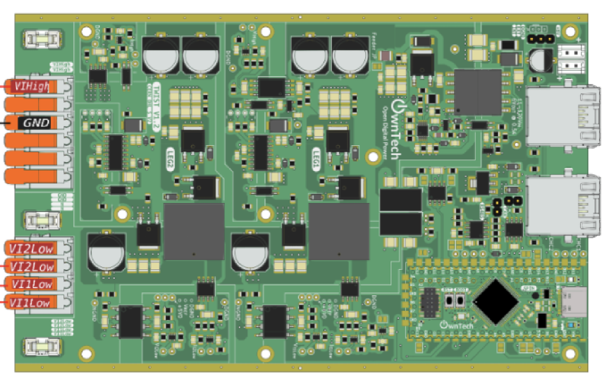
Figure 3: OwnTech’s power converter.

Classically [4], an average state-space model can be obtained by applying Kirchhoff voltage law (KVL) and Kirchhoff current law (KCL) during the two operation modes. The state vector is ${\bf x}=[\;I_{L_{1}}\;\;I_{L_{2}}\;\;V_{C_{1}}\;\;V_{C_{2}}\;\;V_{C_{IN}}\;\;V_{C_{out}}\;]^{T}$, the output is $y=V_{C_{out}}$, the controlled input is the duty-cycle $d(t)\in[0.1,0.9]$ and the disturbance is ${\bf w}=[V_{IN}\;\;\;\delta_{R_{var}}]^{T}$. The average state-space model can be expressed as :

$$\begin{array}[]{rl}{\bf K}\dot{{\bf x}}(t)&=\left({\bf A}_{0}+d(t){\bf A}_{1}\right){\bf x}(t)+\left({\bf B}_{0}+d(t){\bf B}_{1}\right){\bf w}(t)\\ y(t)&={\bf C}{\bf x}(t)\end{array}$$ (1)

The matrices ${\bf K},\ {\bf A}_{0},\ {\bf A}_{1}\in\mathbb{R}^{6\times 6}$, ${\bf B}_{0},\ {\bf B}_{1}\in\mathbb{R}^{6\times 2}$, ${\bf C}\in\mathbb{R}^{1\times 6}$, are given in Table II. Figure 4 shows a comparison of the averaged state-space model (denoted as SSA) from (1) and the Simulink circuit model from the OwnTech Foundation [6] for an open-loop simulation with a constant duty-cycle $d=0.5$.

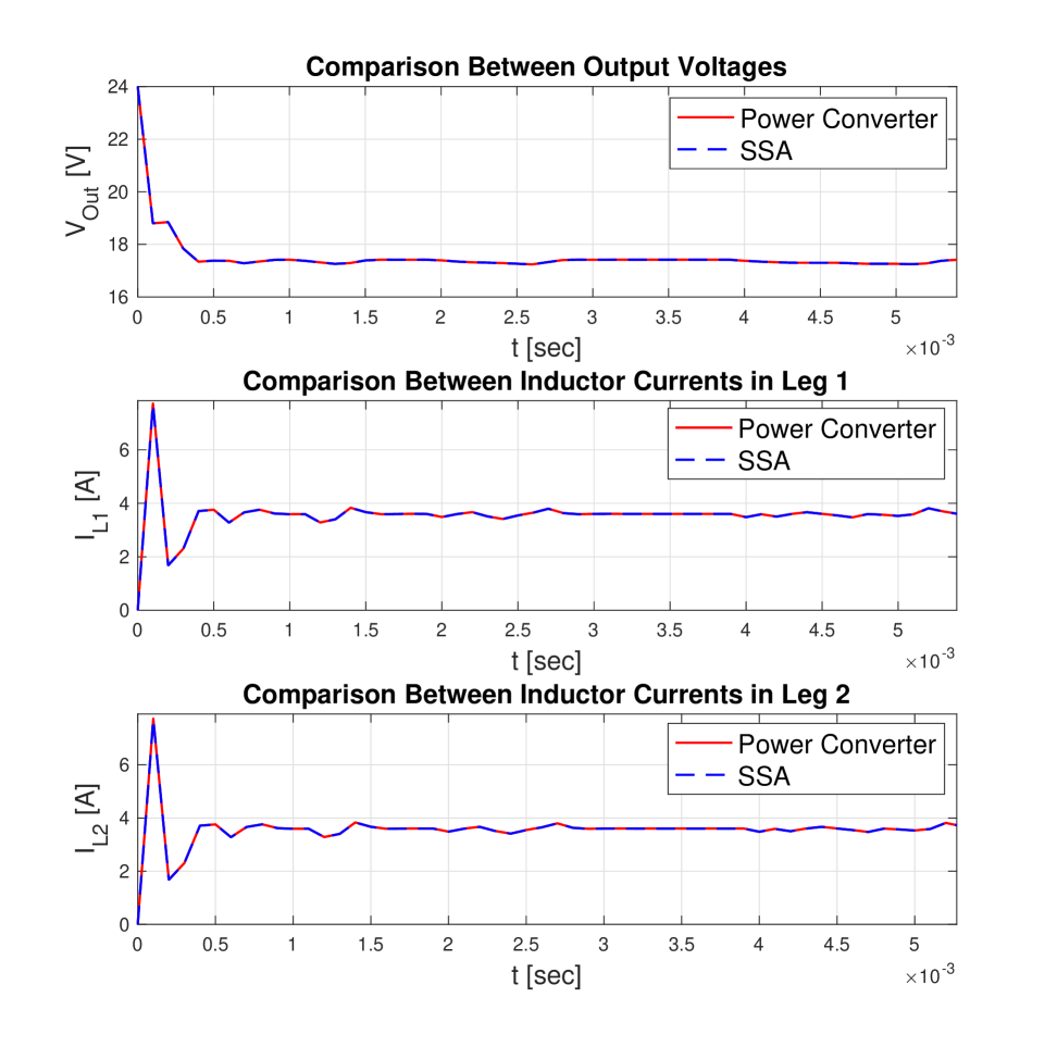
Figure 4: Comparison between SSA model and Power converter

In the present case, this model can be derived without too much difficulties as it remains a simple architecture, but this converter remains a good example of the complexity of the control task as the system is bilinear and subject to input saturation. This is usually handled by linearizing the model around a desired equilibrium point, the control design is then performed on the subsequent linear model. However, this does not allow to ensure that the performance and stability requirements are going to be met when the equilibrium point changes due to variations in the load or the input voltage. Lyapunov-based approach have shown promising results, see [13] for instance, but they control directly the commutations of the switching devices, which make them not suited for PWM-based control, and their scalability is limited as the architecture becomes more complex and the state dimension increases. The next paragraph investigates the use of a data-driven control technique to overcome these challenges.

$$A_{0}=\left[\begin{array}[]{cccccc}-(R_{\text{on}}+R_{c_{1}}\parallel R_{1})&0&-\frac{R_{1}}{R_{c_{1}}+R_{1}}&0&0&-\frac{R_{c_{1}}}{R_{c_{1}}+R_{1}}\\ 0&-(R_{\text{on}}+R_{2}\parallel R_{c_{2}})&0&-\frac{R_{2}}{R_{c_{2}}+R_{2}}&0&-\frac{R_{c_{2}}}{R_{c_{2}}+R_{2}}\\ \frac{R_{1}}{R_{c_{1}}+R_{1}}&0&-\frac{1}{R_{c_{1}}+R_{1}}&0&0&\frac{1}{R_{c_{1}}+R_{1}}\\ 0&\frac{R_{2}}{R_{c_{2}}+R_{2}}&0&-\frac{1}{R_{c_{2}}+R_{2}}&0&\frac{1}{R_{c_{2}}+R_{2}}\\ 0&0&0&-\frac{1}{R_{c}+R_{\text{IN}}}&0&0\\ \frac{R_{c_{1}}}{R_{c_{1}}+R_{1}}&\frac{R_{c_{2}}}{R_{c_{2}}+R_{2}}&\frac{1}{R_{c_{1}}+R_{1}}&\hskip 32.7779pt\frac{1}{R_{c_{2}}+R_{2}}&0&-(\frac{1}{R_{c_{1}}+R_{1}}+\frac{1}{R_{c_{2}}+R_{2}}+\frac{1}{R_{var}})\end{array}\right]$$

$$A_{1}=\left[\begin{array}[]{cccccc}-R_{c}\parallel R_{\text{IN}}&-(R_{c}\parallel R_{\text{IN}})&0&0&\frac{R_{c_{1}}}{R_{c_{1}}+R_{1}}&0\\ -(R_{c}\parallel R_{\text{IN}})&R_{\text{IN}}\parallel R_{c}&0&0&\frac{R_{c_{2}}}{R_{c_{2}}+R_{2}}&0\\ 0&0&0&0&0&0\\ 0&0&0&0&0&0\\ \frac{-R_{\text{IN}}}{R_{c}+R_{\text{IN}}}&\frac{-R_{\text{IN}}}{R_{c}+R_{\text{IN}}}&0&\frac{1}{R_{c}+R_{\text{IN}}}&-\frac{1}{R_{c}+R_{\text{IN}}}&0\\ 0&0&0&0&0&0\end{array}\right]\ \text{with }R_{on}=R_{L_{i}}+R_{MOS_{on}}$$

$$K=\left[\begin{array}[]{cccccc}L_{1}&0&0&0&0&0\\ 0&L_{2}&0&0&0&0\\ 0&0&C_{1}&0&0&0\\ 0&0&0&C_{2}&0&0\\ 0&0&0&0&C_{IN}&0\\ 0&0&0&0&0&C_{out}\end{array}\right],\qquad B_{0}=\left[\begin{array}[]{cc}\frac{R_{c}}{R_{c}+R_{\text{IN}}}&0\\ \frac{R_{c}}{R_{c}+R_{\text{IN}}}&0\\ 0&0\\ 0&0\\ \frac{1}{R_{c}+R_{\text{IN}}}&0\\ 0&1\end{array}\right]\qquad B_{1}=\left[\begin{array}[]{cc}\frac{R_{c}}{R_{c}+R_{\text{IN}}}&0\\ \frac{R_{c}}{R_{c}+R_{\text{IN}}}&0\\ 0&0\\ 0&0\\ 0&0\\ 0&0\end{array}\right]\qquad C=\left[\begin{array}[]{cccccc}0&0&0&0&0&1\end{array}\right]$$

Table II: Matrices of the average state-space model (1)

 

III Data-Driven Control of power converters

The difficulty of traditional model-based control increases as power converters grow more complex. Data-driven control methods offer a promising alternative by designing controllers directly from data without relying on explicit models. In particular, among the various data-driven approaches, Ziegler-Nichols and Virtual Reference Feedback Tuning (VRFT) are popular techniques that are going to be used in this section. The controller $K$ to be designed is a PI of the following form:

$$K(s)=K_{p}+K_{I}\frac{1}{s}$$ (2)

where $K_{p}$ is the proportional gain and $K_{I}$ is the integral gain.

III-A Baseline control using Ziegler-Nichols (ZN) tuning

The Ziegler-Nichols (ZN) method is a heuristic that traces back to the 1940s [14]. The proportional gain is progressively increased until the system exhibits stable and sustained oscillations : the ultimate gain $K_{u}$ and the oscillations period $T_{u}$ are then measured. Several simulations have been conducted on the Owntech Simulink model to get $K_{u}=0.065$ and $T_{u}=1\;[ms]$. The controller gains can then be fixed using the following tuning rule :

$$K_{p}=0.45K_{u}\text{ and }K_{I}=\frac{0.54K_{u}}{Tu}$$ (3)

The ZN tuning rules were initially proposed for the design of a continuous controller for a system that can be approximated by a transfer function of the following type:

$$k\frac{e^{-\tau s}}{s+a}$$ (4)

However, not all systems can be correctly approximated by such transfer function, which constitute the main limitation of the ZN tuning rules and the gains are tuned in a rather aggressive way, which can cause problem when discretizing the controller.

III-B Virtual Reference Feedback Tuning (VRFT)

The VRFT was initially proposed in [3] and with (up to our knowledge) two successful application to power converters in [11] (without anti-windup) and [8] (on a simpler model). The control design is formulated as a controller identification problem by using a reference model to enforce the specifications. This method is entirely data-driven, and only measurements data from a single experiment are needed to get a controller. This process simplifies the controller design process as a precise yet simple enough mathematical model of the system is no longer needed. The principle of VRFT is represented on Figure 5. The objective of VRFT is to design a controller $K$ that closely approximates the ideal controller $K^{\star}$. This ideal controller is the one ensuring that the closed-loop transfer function matches the desired reference model $M$.

Figure 5: Principle of VRFT[3]

The VRFT follows the five steps detailed hereafter :

• Step 1: Data collection

• An experiment is conducted on the power converter, with a user-defined input signal (here the duty cycle signal $d(t)$), and the resulting output voltage $V_{out}(t)$ is collected. In order for the control design to be efficient, the chosen input signal should excites the dynamics to be controlled. In this paragraph, the training data for the VRFT is obtained by an open-loop simulation of the Owntech Simulink model with a chirp duty cycle varying around 0.5 with a frequency varying from $f_{c}/2$ to $2f_{c}$. The collected output is artificially corrupted by a noise signal $\eta(t)$, with $|\eta(t)|\leq 0.5$ . The collected training data is visible on Figures 6 and 7. The dataset used for training consists of $N=501$ samples collected over a simulation duration of 0.05 seconds.

  

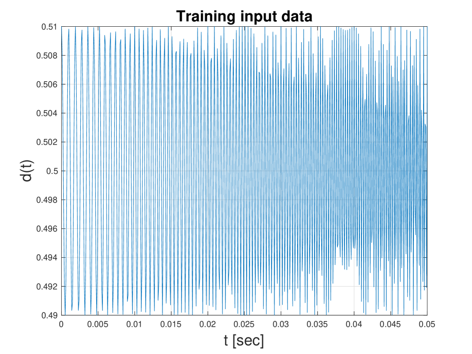
  Figure 6: Input $d(t)$ used for data collection.

  

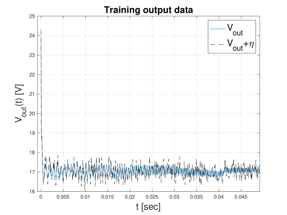
  Figure 7: Collected output $V_{out}(t)$.

• Step 2: Specifications

• The desired reference model $M$ is defined to represent the desired closed-loop behavior. In the present case, a simple first-order model, see (5) is used to enforce a time constant $\tau=\frac{1}{f_{c}}$ corresponding to a desired cut-off frequency $f_{c}$ (here we take $f_{c}=f_{s}/100$ with $f_{s}=1/T_{s}=200kHz$ the switching frequency):

  $$M(s)=\frac{1}{1+s\tau}$$ (5)

  The reference model is discretized using the ZOH method with a sampling time $T_{samp}=100\;[\mu\;s]$. It should be noted that the choice of a reference model can be tricky when the system to be controlled is unstable or non-minimum phase, see [15].

• Step 3: Control structure

• The controller to be tuned is expressed as $K(z,\theta)=\beta^{T}(z)\theta$, where $\beta(z)$ defines the structure of the controller and is defined in discrete time. The parameters to be optimized are grouped in the vector $\theta$. In the present case, the controller is a PI, which gives $\theta=[K_{p}\;\;K_{I}]^{T}$ and

  $$\beta^{T}=\begin{bmatrix}1&\frac{z}{z-1}\end{bmatrix}$$ (6)

  It should be noted that, in theory, the control structure $\beta(z)$ should be chosen so that it can approximates correctly the ideal controller $K^{\star}$, which is a complicated task when the system to be controlled is unknown and/or complex.

• Step 4: Control tuning

• First, the virtual reference signal $r(t)$ is constructed so to satisfy $V_{out}(t)=M(z)\cdot r(t)$. It corresponds to the reference that would have been sent to the desired closed-loop model in order to get the training output $V_{out}(t)$. The corresponding virtual tracking error $e(t)=r(t)-V_{out}(t)$ is then computed. The ideal controller $K^{\star}$ is then the one that gives the training signal $d(t)$ when it is fed with the virtual error $e(t)$ : this is how the control tuning problem is recast as controller identification.

  

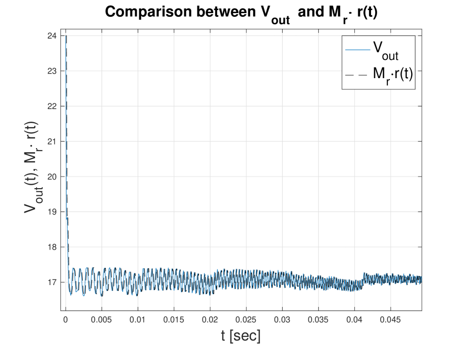
  Figure 8: Comparison between $V_{out}(t)$ and $M\cdot r(t)$

  The controller parameters $\theta=[K_{p}\;\;K_{I}]^{T}$ are then found by minimizing the following criterion

  $$J_{VRFT}=\frac{1}{N}\sum_{t=1}^{N}(d(t)-K(z;\theta)\cdot e(t))^{2}$$ (7)

  $$=\frac{1}{N}\sum_{t=1}^{N}(d(t)-\Phi^{T}(t)\cdot\theta)^{2}$$

  Knowing that $K(z,\theta,)=\beta^{T}(z)\theta$, the regressor is $\Phi(t)=\beta(z)e(t)$. This is a least squares problem that can be solved easily. The solution $\theta^{\star}$ is given by:

  $$\theta^{\star}=[\sum_{t=1}^{N}\Phi(t)\cdot\Phi(t)]^{-1}\sum_{t=1}^{N}\Phi(t)\cdot d(t)$$ (8)

  In the end, the following parameters are estimated :

  $$\theta^{\star}=\left[K_{p}^{\star}\ K_{I}^{\star}\right]^{T}=\left[0.0031\;\;0.0065\right]^{T}$$

  After discretization, the PI controller implemented in the Simulink model is the following :

  $$K(s)=0.0031+0.0065\cdot\frac{T_{s}}{s}$$ (9)

Figure 9 show the performances of the ZN and VRFT controllers for a constant $V_{out}^{ref}=10[V]$ and the corresponding control signals are represented on Figure 10. While one can see that the VRFT controller performs better than the ZN one with a faster response, a significant undershoot is observed for both controllers.

The duty cycle of the OwnTech converter is constrained within the range $[0.1,0.9]$ (see Figure 2), which explains the large undershoot observed in Figure 9 : this is due to the saturation of the duty cycle observed in Figure 10. This phenomenon is known as windup, and it is commonly encountered with PI controllers. When the controller output exceeds the duty cycle saturation limit, the integral term continues to accumulate the error, resulting in an integrated error buildup. As noted in [7], this issue becomes critical as the accumulated error can lead to significant undershoot and, in some cases, may cause unstable behavior. In the present case, the ZN controller leads to a longer saturation than the VRFT one.

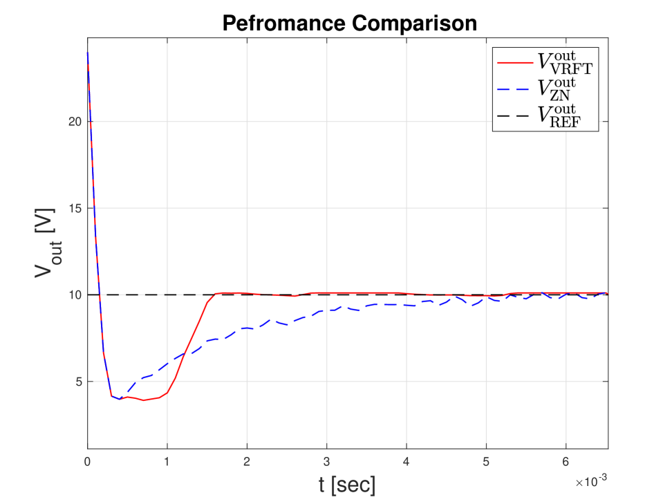
Figure 9: Closed-loop performance comparison between the ZN and VRFT controllers with a constant reference signal

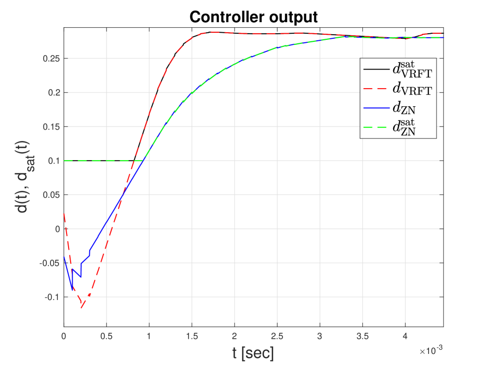
Figure 10: Comparison between the ZN and VRFT controllers’ output with the saturated duty cycle.

III-C Extended VRFT With Anti-Windup Compensation

In order to improve the closed-loop performances, an anti-windup compensation is included in the designed controller, following the VRFT extension proposed in [12]. Anti-windup is commonly used in control systems to prevent the integrator from accumulating error when the controller output becomes saturated. While there are several anti-windup methods, the one adopted here [5] uses the difference between the saturated input and the actual control input to regulate the behavior of the integral action in order to avoid windup phenomenon. Such control structure is illustrated on Figure 11. The duty cycle $d_{sat}(t)$ that is actually sent to the power converter is given by :

$$d_{sat}(t)=\begin{cases}0.9&\text{if }d(t)>0.9\\ 0.1&\text{if }d(t)<0.1\\ d(t)&\text{otherwise}\end{cases}$$ (10)

Figure 11: The PI controller with Anti-Windup

As shown in Figure 11, the controlled output $d(t)$ is given by:

$$d(t)=(K_{p}\cdot e(t))+K_{I}\int e(t)dt+K_{I}K_{AW}\sum_{j=1}^{n_{Aw}}u_{d}(t-j)$$ (11)

where $u_{d}=d-d_{sat}$ represents the anti-windup term. It allows to act on the control signal only when the PWM generator saturates, in which case $u_{s}\neq 0$ while $u_{d}=0$ otherwise. The design parameter $n_{AW}$ determines how many past values of $u_{d}$ are taken into account in the anti-windup compensation. As in [5], $n_{AW}=1$ is selected, which is often sufficient. A larger $n_{AW}$can be selected for slow systems where saturation effects persist over multiple time steps, but it increases computational complexity and the number of parameters to tune.

Compared to the classical VRFT approach recalled in the previous paragraph, the collected data includes now the signal $u_{d}$ in addition to the input-output measurements. Note that to design the ant-windup compensation, it is necessary that the training experiment hits saturation. For this reason, compared to the previous paragraph, the training data set is modified and is visible on Figures 12, 13 and 14. The data collection simulation is perfomed in open-loop, with a chirp input signal $d(t)$ spanning the same frequency range as before, but around a fixed operating point of $0.15$ to ensure that the duty cycle goes below the saturation limit $0.1$, leading to the occurrence of the windup phenomenon which is part of the dynamics to be controlled (see the traing set for $u_{d}$ on Figure 14.

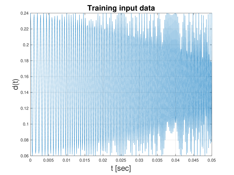
Figure 12: Input $d(t)$ used for data collection for the VRFT design including anti-windup compensation.

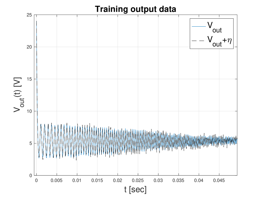
Figure 13: Collected output $V_{out}(t)$ for the VRFT design including anti-windup compensation.

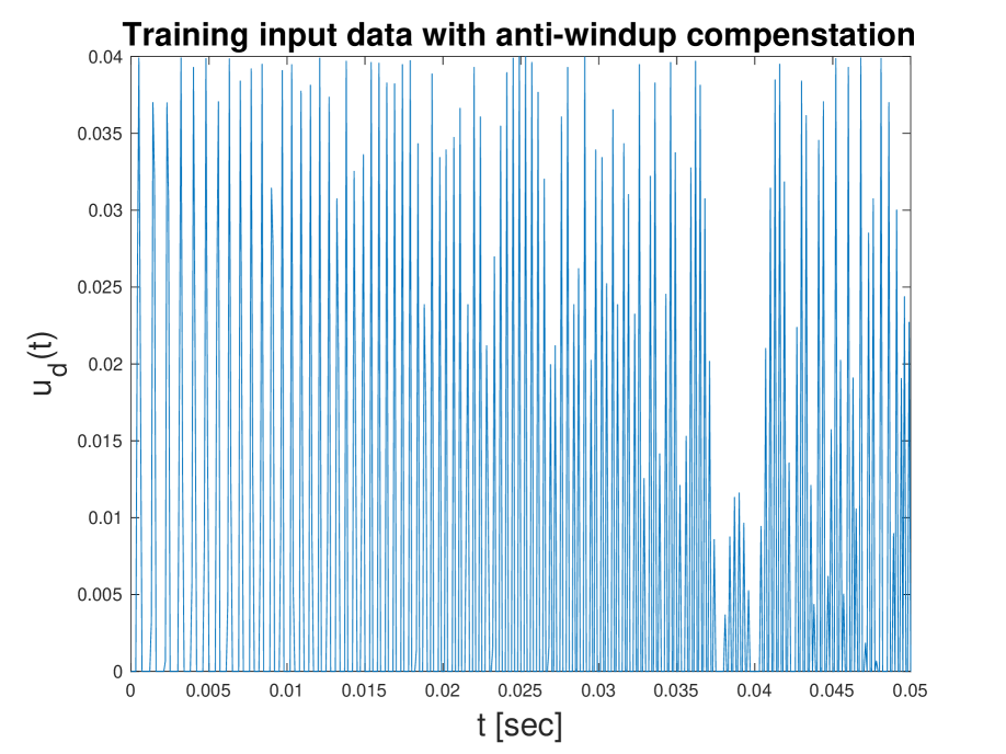
Figure 14: Collected new controller input $u_{d}(t)$ for the VRFT design including anti-windup compensation.

The controller structure $\beta(z)$ is also changed to include the anti-windup compensation from Figure 11. The virtual reference $r$ and the virtual tracking error $e$ are then computed as previously. The problem can then be formulated as a least-squares problem as in Step 4 of the classical VRFT, but with new regressors :

$$J_{VRFT,AW}(\theta_{AW})=||d-\Phi_{AW}\theta_{AW}||^{2}$$ (12)

with the regression matrix $\Phi_{AW}$ is :

$$\Phi_{AW}(t)=\begin{bmatrix}e_{(}t)&\int e(t)dt&u_{d}(t-1)\end{bmatrix}^{\top}$$ (13)

and the parameters to be estimated $\theta_{AW}$ :

$$\theta_{AW}=[K_{p}\;\;\;K_{i}\;\;\;K_{AW}K_{i}]^{T}$$ (14)

The optimal parameter vector $\theta_{AW}$ that minimizes (12) is then given by:

$$\theta_{AW}^{\star}=[\sum_{t=1}^{N}\Phi_{AW}(t)\Phi_{AW}(t)]^{-1}\sum_{t=1}^{N}\Phi_{AW}(t)d(t).$$ (15)

The estimated controller has the following gains :

$$K_{p}^{\star}=0.0018,\ K_{I}^{\star}=0.0056\text{ and }K_{AW}^{\star}=441.47$$ (16)

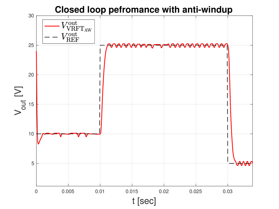
Figure 15: Closed-loop performance with anti-windup implementation

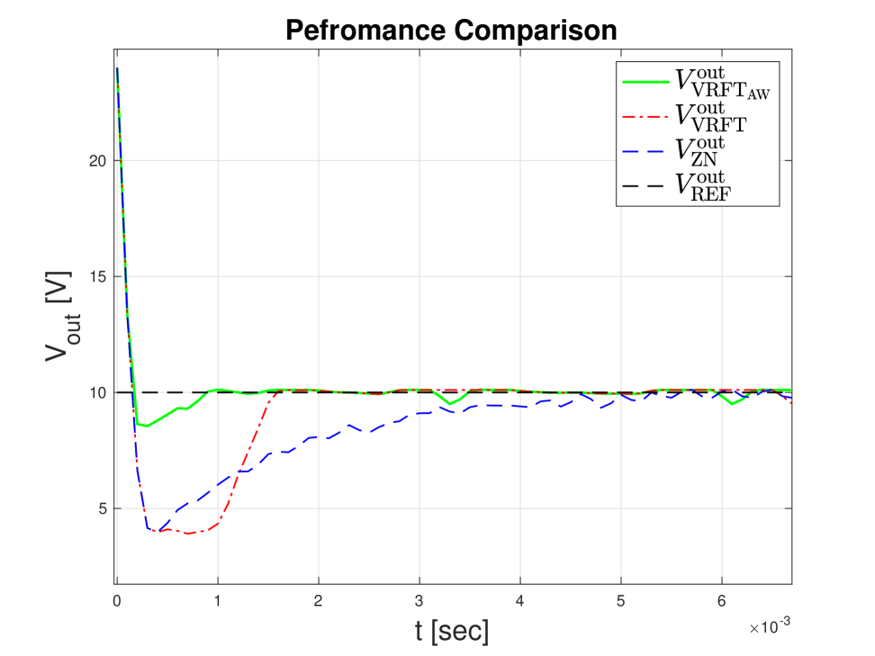
Figure 16: Closed-loop performance comparison

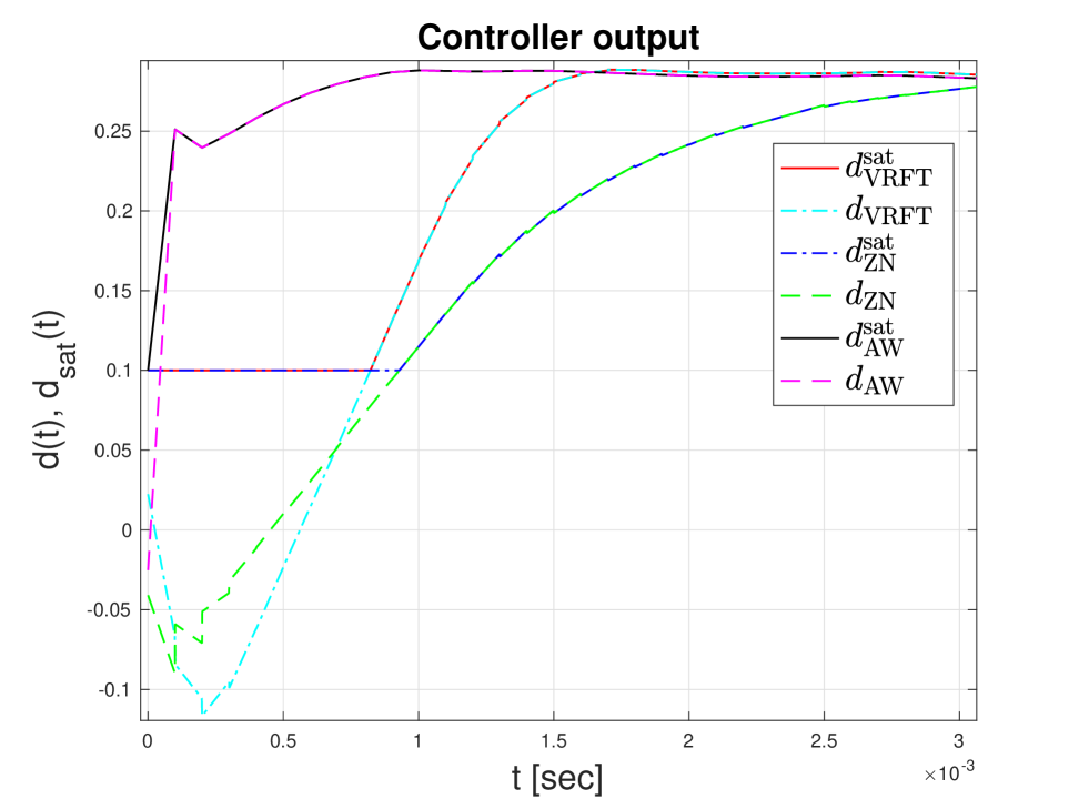
Figure 17: Comparison between the controllers’ output with the saturated duty cycle.

As visible on Figures 16 and Figure 17, the tracking error is reduced by including an anti-windup compensation, which allows to adjust the integral gain. Performances of the different designed controllers are summarized in Table III, showing that the VRFT data-driven approaches used in this paper outperform the baseline controller obtained by the ZN tuning rules (the performance indicators are calculated on the first transient to reach $V_{out}^{ref}=10V$, see Figure 16).

Table III: Closed-loop performance comparison between the different control designs

Controller	Undershoot (%)	Settling Time $5\%$ (ms)
$C_{ZN}$	61	2.7
$C_{VRFT}$	60.8	1.8
$C_{VRFT_{AW}}$	11.4	0.9

IV Conclusion

This work details the data-driven control design of a power converter using VRFT [3] and its anti-windup extension [5]. On the presented example, a simple and reproducible choice of hyperparameters allow to obtain a PI controller, with or without anti-windup compensation, from a single set of input-output measurements. The performances are better than the considered baseline controller obtained through the Ziegler-Nichols tuning rules.

Future work should focus on the experimental validation of the proposed method to confirm its practical effectiveness, in particular on more complex architecture. Additionally, investigating the performance of these techniques under more dynamic and challenging operating conditions would be an interesting research path. Indeed, while this approach allows an easy and quick control tuning, there is no stability nor performance guarantees contrary to Lyapunov-based approaches. In the case of linear systems, this is enforced in data-driven control procedure through the choice of reference model, training dataset and controller structure. The underlying theoretical and methodological problem is then to extend this understanding to the case of nonlinear systems.

References

- [1] J. Hu, Y. Shan, K. W. Cheng, and S. Islam, Overview of power converter control in microgrids—challenges, advances, and future trends, IEEE Transactions on Power Electronics, 2022.
- [2] F. Blaabjerg, Control of power electronic converters and systems, Elsevier Science Edition, 2018.
- [3] M. C. Campi, A. Lecchini, and S. M. Savaresi, Virtual reference feedback tuning: A data-driven method for the design of feedback controllers, Automatica, 2002.
- [4] R. W. Erickson and D. Maksimovic, Fundamentals of power electronics, 2nd edition, Springer, 2001.
- [5] V. Breschi and S. Formentin, Direct data-driven control with embedded anti-windup compensation, Proceedings of Machine Learning Research, 2020.
- [6] OwnTech Foundation, Power converter "TWIST" model, Online GitHub Repository, https://gitlab.laas.fr/owntech/models/simscape-power-system/buck-converter/-/tree/erouxpalom-main-patch-08779?ref_type=heads
- [7] J. W. Choi and S. C. Lee, Antiwindup strategy for PI-type speed controller, IEEE Transactions on Industrial Electronics, 2009. https://doi.org/10.1109/TIE.2008.2004073
- [8] N. Kameya, Y. Hosoyamada, Y. Fujimoto, and T. Suenaga, VRFT for Current-Mode Buck Converter with Anti-Windup Compensation, IEEE Energy Conversion Congress and Exposition (ECCE), 2022.
- [9] I. Markovsky, L. Huang, and F. Dörfler, Data-driven control based on the behavioral approach: From theory to applications in power systems, IEEE Control Systems Magazine, 2023.
- [10] Z.S. Hou and Z. Wang, From model-based control to data-driven control: Survey, classification and perspective, Information Sciences, 2013.
- [11] C. L. Remes, R. B. Gomes, J. V. Flores, F. B. Líbano, L. Campestrini, Virtual reference feedback tuning applied to DC–DC converters. IEEE Transactions on Industrial Electronics, 2020.
- [12] V. Breschi, S. Formentin, Direct data-driven control with embedded anti-windup compensation. Learning for Dynamics and Control, 2020.
- [13] S. Ahmad, R. P. C. d. Souza, P. Kergus, Z. Kader and S. Caux, Estimation-Based Robust Switching Control of a DC-DC Boost Converter, in IEEE Transactions on Industry Applications, 2025.
- [14] J.G. Ziegler, N. b. Nichols, Optimum settings for automatic controllers, in Transactions of the ASME, 1942.
- [15] P. Kergus, M. Olivi, C. Poussot-Vassal and F. Demourant, From Reference Model Selection to Controller Validation: Application to Loewner Data-Driven Control, in IEEE Control Systems Letters, 2019.