Fast Wasserstein rates for estimating probability distributions of probabilistic graphical models

Abstract

Using i.i.d. data to estimate a high-dimensional distribution in Wasserstein distance is a fundamental instance of the curse of dimensionality. We explore how structural knowledge about the data-generating process which gives rise to the distribution can be used to overcome this curse. More precisely, we work with the set of distributions of probabilistic graphical models for a known directed acyclic graph. It turns out that this knowledge is only helpful if it can be quantified, which we formalize via smoothness conditions on the transition kernels in the disintegration corresponding to the graph. In this case, we prove that the rate of estimation is governed by the local structure of the graph, more precisely by dimensions corresponding to single nodes together with their parent nodes. The precise rate depends on the exact notion of smoothness assumed for the kernels, where either weak (Wasserstein-Lipschitz) or strong (bidirectional Total-Variation-Lipschitz) conditions lead to different results. We prove sharpness under the strong condition and show that this condition is satisfied for example for distributions having a positive Lipschitz density.

Keywords: probabilistic graphical models, nonparametric estimation, Wasserstein distance.

AMS 2010 Subject Classification: 62A09; 62G05; 68T30; 62G30

1 Introduction

Overcoming the curse of dimensionality in high-dimensional learning settings usually requires inductive biases, i.e., some a priori assumptions on the kind of structures one tries to learn. One of the basic learning settings of this kind is non-parametric estimation of probability measures, which aims at learning the distribution of high-dimensional random variables without parametric assumptions (see, e.g., [12, 16, 40]). Most approaches towards overcoming the curse of dimensionality in this setting have focused on imposing biases towards smoothness, often explicitly by working with distributions having smooth Lebesgue densities (see, e.g., [33, 40]) or also implicitly through the kind of distance used to measure the difference of the estimate from the truth (see, e.g., [23, 39]). In this paper, we provide complementary results by focusing on biases related to the relational structure between the different variables of the distributions (cf. [5]). More precisely, we focus on distributions of probabilistic graphical models (see, e.g., [24, 35]) corresponding to a known graph such that the kernels occurring in the disintegration according to the graph are continuous in a suitable sense. With this setting, we aim to accomplish two things: First, establish conditions for large random systems which guarantee that the rate of estimation only depends on local parts of the system. And second, introducing smoothness criteria based on stochastic kernels instead of Lebesgue densities to cover settings with partly discrete variables as well.

1.1 Setting and summary of the main results

1.1.1 General learning setting

Let $\mathcal{X}=[0,1]^{d}$, denote by $\mathcal{P}(\mathcal{X})$ the set of probability measures on $\mathcal{X}$ and set $\mathcal{W}$ to be the first order Wasserstein distance on $\mathcal{P}(\mathcal{X})$, defined by

$$\mathcal{W}(\mu,\nu)=\inf_{\pi}\int_{\mathcal{X}\times\mathcal{X}}\|x-y\|\,\pi(dx,dy),$$

where the infimum is taken over all couplings $\pi$, i.e. measures $\pi$ with first marginal $\mu$ and second marginal $\nu$. Throughout, we use $\|\cdot\|=\|\cdot\|_{\infty}$, which is of course only relevant up to constants. We refer e.g. to [19, 43] for background on Wasserstein distances.

We are interested in estimating a probability measure $\mu\in\mathcal{P}(\mathcal{X})$ via $n$ i.i.d. samples $X^{1},\dots,X^{n}$ selected according to $\mu$, that is, find an estimator $E_{n}:\mathcal{X}^{n}\rightarrow\mathcal{P}(\mathcal{X})$ such that

$$\int\mathcal{W}(\mu,E_{n})\,d\mu^{\otimes n}=\int\mathcal{W}(\mu,E_{n}(x^{1},\dots,x^{n})\,\mu(dx^{1})\ldots\mu(dx^{n})$$

is small simultaneously for many different distributions $\mu$ in a set $\mathcal{Q}\subseteq\mathcal{P}(\mathcal{X})$. Hence, we wish to solve

$$V_{Q}(n):=\inf_{E_{n}}\sup_{\mu\in\mathcal{Q}}\int\mathcal{W}(\mu,E_{n})\,d\mu^{\otimes n}.$$ (1.1)

In the case where one does not impose any additional prior knowledge and thus works with $\mathcal{Q}=\mathcal{P}(\mathcal{X})$ for $d\geq 3$, it is well known that $V_{Q}(n)\lesssim n^{-1/d}$ (see [12] and also [16]). Notably, these rates are attained by the empirical measure $E_{n}(x^{1},\dots,x^{n})=\frac{1}{n}\sum_{i=1}^{n}\delta_{x^{i}}$. In this case, no estimator can do better, and so $V_{Q}(n)\gtrsim n^{-1/d}$ holds as well (see, e.g., [9]). With additional structural assumptions, that is, when $\mathcal{Q}\subsetneq\mathcal{P}(\mathcal{X})$, the empirical measure is usually suboptimal and other estimators must be used to obtain optimal rates (cf. [33, 40]).

1.1.2 Probabilistic graphical models

Throughout this paper, we always assume that a directed acyclic graph $G$ with nodes $\{1,\dots,K\}$ is given (and known to the statistician) and is topologically sorted, which means that there are no edges from $i$ to $j$ for $j<i$. The space $\mathcal{X}=[0,1]^{d}$ is partitioned into $\mathcal{X}=\mathcal{X}_{1}\times\dots\times\mathcal{X}_{K}$ where $\mathcal{X}_{k}=[0,1]^{d_{k}}$ and $\sum_{k=1}^{K}d_{k}=d$. For $x\in\mathcal{X}$, denote by $x_{k}\in\mathcal{X}_{k}$ the projection onto the $k$-th coordinate, and by $x_{I}$ the projection onto a subset of variables $I\subseteq\{1,\dots,K\}$. Further, denote by $\text{\rm pa}(k)$ the set of parent nodes of a node $k$. Probabilistic graphical models for the graph $G$ are defined as

$$\mathcal{P}_{G}:=\left\{\mu\in\mathcal{P}(\mathcal{X})\mid\mu(dx_{1},\dots,dx_{K})=\prod_{k=1}^{K}\mu(dx_{k}\mid x_{\text{\rm pa}(k)})\right\}.$$

That is, when integrating the $k$-th variable in the disintegration of $\mu\in\mathcal{P}_{G}$, one only needs to condition on the parent variables of $k$ according to $G$. One simple example of a relevant graph is $1\rightarrow 2\rightarrow\ldots\rightarrow K$, in which case $\mathcal{P}_{G}$ corresponds to distributions of Markov chains. Whenever $\text{\rm pa}(k)$ is empty, the conditional distribution is just understood as the marginal distribution. For instance since $\text{\rm pa}(1)=\emptyset$, $\mu(dx_{1}\mid x_{\text{\rm pa}(1)})$ is just the first marginal of $\mu$. We mention that $\mu\in\mathcal{P}_{G}(\mathcal{X})$ can analogously be defined using conditional independences (see, e.g., [8, Remark 3.2]).

Probabilistic graphical models are also known as Bayesian networks and naturally related to Bayesian inference (cf. [22]). They are more generally used to combine structural assumptions about data generating processes with probabilistic modelling tools. This is important to express and infer causal probabilistic relations, for instance in fields like environmental modelling (cf. [29]), biology (cf. [25]) or climate research (cf. [13]). They are further used to bridge the gap between causality and machine learning (cf. [37]) and thus naturally occur in the study of modern machine learning architectures (see, e.g., [31, 44]). We refer to [24, 34, 35] for more background on probabilistic graphical models.

1.1.3 Lower bounds without continuous kernels

The first natural idea is to explore the learning problem (1.1) with $Q=\mathcal{P}_{G}$. We find that this is, however, not a fruitful approach. Aside from trivial cases in which the graph $G$ has disconnected components and thus one can estimate those components separately, it is not obvious at all how the prior knowledge of $\mu\in\mathcal{P}_{G}$ is beneficial compared to $\mu\in\mathcal{P}(\mathcal{X})$. To explain these difficulties, it might be helpful to think of $\mathcal{P}_{G}$ as an analogue of the set of all distributions having a Lebesgue density, but without any quantitative control on the smoothness of this density. With this point of view, it is natural that the prior knowledge of $\mu\in\mathcal{P}_{G}$ is statistically not helpful, similarly to how knowledge of the existence of a Lebesgue density alone is not helpful.

And indeed, we establish in Section 4 that for many graph structures, the set $\mathcal{P}_{G}$ is dense in $\mathcal{P}(\mathcal{X})$ with respect to weak convergence, and the learning problem (1.1) using $Q=\mathcal{P}_{G}$ still has the rate $n^{-1/d}$. This involves all graphs which have only one root node, as for instance the Markovian graph $1\rightarrow 2\rightarrow\ldots\rightarrow K$, or any kind of tree, see Theorem 4.2 and Corollary 4.3. The reason is that those graph structures do not impose any kind of unconditional, but only conditional independences, which we show in Theorem 4.2 to be, as a purely qualitative assumption, statistically useless. To complement this result, we also explore another graph structure which can be regarded as an extreme case in terms of imposing several unconditional independences, namely the graph only including the nodes $k\rightarrow K$ for $k\in\{1,\dots,K-1\}$. In this graph all nodes $\{1,\dots,K-1\}$ are independent, and we establish in Proposition 4.4 that the rate is again $n^{-1/d}$ in this case.

While we do not establish the lower bound $n^{-1/d}$ for all graphs having only one connected component, we believe the covered cases provide evidence that, for statistical purposes, one should quantify the compatibility of a probability measure $\mu$ with a graph $G$ instead of merely working with $\mathcal{P}_{G}$.

1.1.4 Fast (and sharp) rates under continuous kernels

To quantify how well a probability measure is compatible with a graph $G$, we introduce Lipschitz continuity conditions on the stochastic kernels occurring in the definition of $\mathcal{P}_{G}$. More precisely, we shall consider two different conditions, one where Lipschitz continuity of the kernels is formulated via the Wasserstein distance, and one via the total variation distance.

In both cases, the construction for the estimators we use requires certain conditions on the graphical structures. To state this assumption, recall that a subset $J$ of the nodes of the graph $G$ is called fully connected if there is an edge $k\rightarrow\ell$ for all $k,\ell\in J$ with $k<\ell$.

Assumption 1.1.

The graph $G$ contains no colliders, that is, for any $k\in\{1,\dots,K\}$, the set $\text{\rm pa}(k)$ is fully connected.

We shortly mention that any graph can be transformed to one which satisfies Assumption 1.1 simply by adding edges, and adding edges to a graph can never destroy compatibility of a probability measure with the graph. However, we will see below that more edges translate to a possibly worse rate of convergence, which is of course undesirable. In other words, Assumption 1.1 can be circumvented, albeit at the cost of a possibly worse rate of convergence.

Kernels which are Wasserstein-Lipschitz. The kernels corresponding to the disintegration of the graph are given by the maps

$$\mathcal{X}_{\text{\rm pa}(k)}\ni x_{\text{\rm pa}(k)}\mapsto\mu(dx_{k}\mid x_{\text{\rm pa}(k)})\in\mathcal{P}(\mathcal{X}_{k}).$$

The most natural approach to impose continuity for these maps is to use the Wasserstein distance on $\mathcal{P}(\mathcal{X}_{k})$, leading to the following assumption.

Assumption 1.2.

$\mu\in\mathcal{P}_{G}(\mathcal{X})$ satisfies

$$\mathcal{W}(\mu(dx_{k}\mid x_{\text{\rm pa}(k)}),\mu(dx_{k}\mid\tilde{x}_{\text{\rm pa}(k)})) \leq L\|x_{\text{\rm pa}(k)}-\tilde{x}_{\text{\rm pa}(k)}\|,$$

for all $2\leq k\leq K$ and for all $x_{\text{\rm pa}(k)},\tilde{x}_{\text{\rm pa}(k)}\in\mathcal{X}_{\text{\rm pa}(k)}$.

To formulate the main result in the setting of Wasserstein-Lipschitz kernels, set $d_{\text{\rm pa}(k)}=\sum_{\ell\in\text{\rm pa}(k)}d_{\ell}$ and define the local dimension $d_{\rm loc}$ as

$$d_{\rm loc}=\max_{k=1,\dots,K}\left(\max\{2,d_{k}\}+d_{\text{\rm pa}(k)}\right).$$ (1.2)

The following showcases that for graphical models with Lipschitz kernels, the overall rate of estimation no longer depends on the overall dimension $d$, but on the local dimension $d_{\rm loc}$ instead.

Theorem 1.3.

Assume $G$ satisfies Assumption 1.1, fix $L>0$ and denote by $\mathcal{Q}$ the set of measures $\mu\in\mathcal{P}_{G}$ which satisfy Assumption 1.2 with constant $L$. Then, there exists a constant $C$ depending only on $G$, $L$ and $d_{\rm loc}$ such that

$$V_{Q}(n)\leq C\,\max\{\log(n),1\}\,n^{-1/d_{\rm loc}}.$$

Proof.

The result follows from Theorem 2.2. ∎

Two brief comments are in order: First, the estimator used to obtain the given upper bound is simple and tractable. Most importantly, the resulting estimate is still a discrete distribution and the computation involves no optimization, merely recombining samples in a suitable way. Second, the $\log(n)$-factor is actually only necessary if $d_{\rm loc}$ is attained at $d_{k}=2$, and the constant $C$ is explicitly tractable (arising mainly from Lemma 2.4).

While Theorem 1.3 gives a simple way to exploit the graphical structure and leads to rates depending only on the local dimension, it is open whether the given continuity condition is used optimally by our estimator—that is, whether the given rates are sharp. Indeed, even in the simple case with two nodes and the graph $1\rightarrow 2$, with $d_{1}=d_{2}=3$, we could not establish a matching lower bound on the rate.

Kernels which are Total Variation-Lipschitz. To move towards faster rates which are sharp, we work under a stronger (yet, as we shall explain, natural) continuity assumption on the stochastic kernels. Denote by ${\rm TV}$ the total variation distance, that is, ${\rm TV}(\nu,\tilde{\nu})=\sup_{f}(\int f\,d\nu-\int f\,d\tilde{\nu})$ where the supremum is taken over all measurable functions $f$ satisfying $|f|\leq 1/2$. In the setting of this paper, we always have that the Wasserstein distance is upper bounded by the total variation distance, which leads to the following strengthening of Assumption 1.2: To formulate it, we write $\text{\rm pre}(k):=\{1,\ldots,k\}\setminus\text{\rm pa}(k)$.

Assumption 1.4.

$\mu\in\mathcal{P}_{G}(\mathcal{X})$ satisfies

$${\rm TV}(\mu(dx_{k}\mid x_{\text{\rm pa}(k)}),\mu(dx_{k}\mid\tilde{x}_{\text{\rm pa}(k)})) \leq L\|x_{\text{\rm pa}(k)}-\tilde{x}_{\text{\rm pa}(k)}\|,$$

$${\rm TV}(\mu(dx_{\text{\rm pre}(k)}\mid x_{\text{\rm pa}(k)}),\mu(dx_{\text{\rm pre}(k)}\mid\tilde{x}_{\text{\rm pa}(k)})) \leq L\|x_{\text{\rm pa}(k)}-\tilde{x}_{\text{\rm pa}(k)}\|,$$

for all $2\leq k\leq K$, $x_{\text{\rm pa}(k)},\tilde{x}_{\text{\rm pa}(k)}\in\mathcal{X}_{\text{\rm pa}(k)}$ and, for all $x_{k},\tilde{x}_{k}\in\mathcal{X}_{k}$,

$${\rm TV}(\mu(dx_{\text{\rm pa}(k)}\mid x_{k}),\mu(dx_{\text{\rm pa}(k)}\mid\tilde{x}_{k})) \leq L\|x_{k}-\tilde{x}_{k}\|.$$

Intuitively, the first inequality of Assumption 1.4 states that small changes in the cause (the parents $\text{\rm pa}(k)$) lead to small changes in the effect’s (the node $k$) distribution, while the other conditions mean that the distribution of the cause remains stable under varying observed effects. Though the second may seem less intuitive at first, it can be viewed as a form of stable Bayesian updating—a natural assumption. For instance for a Markov graph $1\rightarrow 2\rightarrow\ldots\rightarrow K$, one quickly checks that Assumption 1.4 reduces to both the conditional distributions $\mu(dx_{k}\mid x_{k-1})$ and $\mu(dx_{k-1}\mid x_{k})$ being Lipschitz. We also show in Lemma 3.1 that Assumption 1.4 is satisfied for general graphs whenever $\mu$ has a Lipschitz continuous density bounded from below.

The following is the main result of this section and the paper, showcasing the estimation under the strengthened Lipschitz condition. To this end, set $d_{\rm max}:=\max_{1\leq k\leq K}\max\{2,d_{k}\}$.

Theorem 1.5.

Assume $G$ satisfies Assumption 1.1, fix $L>0$ and denote by $\mathcal{Q}$ the set of measures $\mu\in\mathcal{P}_{G}$ which satisfy Assumption 1.4 with constant $L$. Then, there exists a constant $C$ depending only on $G$, $L$ and $d_{\rm loc}$ such that

$$V_{\mathcal{Q}}(n)\leq C\cdot\max\{\log(n),1\}\left(n^{-2/(2+d_{\rm loc})}+n^{-1/d_{\rm max}}\right).$$

Proof.

The result follows from Theorem 3.3. ∎

We emphasize again, as in Theorem 1.3, that the $\log(n)$-factor is only needed in cases when $d_{k}=2$ leads to the dominant terms in $d_{\rm loc}$, and that the estimator achieving the given rate is highly tractable and discrete. More importantly and in contrast to Theorem 1.3, the established rate in Theorem 1.5 is actually sharp! (At least up to the $\log(n)$ term.)

Proposition 1.6.

In the setting of Theorem 1.5: Suppose further that $d_{\rm loc}$ is attained for some $k$ satisfying $d_{k}\geq 2$. Then, there exists an absolute constant $C>0$ such that

$$V_{\mathcal{Q}}(n)\geq C\left(n^{-2/(2+d_{\rm loc})}+n^{-1/d_{\rm max}}\right).$$

The proof of the result is given at the end of Section 3. We emphasize that the inclusion of the term $n^{-1/d_{\rm max}}$ is clearly necessary, as no restrictions on the marginal distributions for each node is imposed. The sharpness of the term $n^{-2/(2+d_{\rm loc})}$ builds on lower bounds for density estimation under Lipschitz conditions. In this context, we emphasize that Theorem 1.5 is novel even for the graph $1\rightarrow 2$; that is, even without the focus on the graphical structure, but merely focusing on the smoothness aspect, the given result provides new conditions for sharp rates.

1.1.5 Structure of the paper

The remainder of the paper is structured as follows: We start by shortly reviewing additional related literature. In Section 2, we work in the setting when (forward-)kernels are Lipschitz with respect to the Wasserstein distance. Section 2 also serves as a warm-up for Section 3 which contains our main results, namely about sharp rates in the setting when (forward and backwards)-kernels are Lipschitz with respect to the total variation distance. Section 4 establishes the lower bounds for $\mathcal{P}_{G}$ without continuity assumptions on the kernels.

1.2 Related Literature

Upper bounds for empirical measures for the $p$-th order Wasserstein distance are a classical topic in probability theory and statistics and are established for instance in [12, 16]. A general approach to establish lower bounds is given in [40] and using smoothness of densities to improve Wasserstein estimation rates is established in [33].

Another line of work focuses on using weaker notions of distances which do not exhibit the curse of dimensionality, for instance through integral probability metrics under smooth test functions (e.g., [23, 39]; IPMs notably include the Sinkhorn divergence, cf. [17]), low-dimensional projections (e.g., [4, 28, 32]) or smoothed versions of Wasserstein distances (e.g., [18]). We refer to [9, Sections 2.7 and 2.8] for a detailed overview.

The recent works [21, 41] also focus on improved estimation rates of distributions under structural assumptions. They explore estimating smooth densities under additional decomposition assumptions on the densities, and thus the goal of reducing to a local notion of complexity is the same as in this paper, the used distances and smoothness assumptions are however very different.

In [3], the authors focus on statistical estimation under a stronger notion of Wasserstein distance focusing on differences between stochastic processes by comparing kernels forward in time. A similar goal of learning conditional distributions is pursued in [1, 6]. The techniques in Section 2 build on the ones used in [3], in particular a similar result to Theorem 1.3 in the particular case where the graph arises from a Markov-chain is given by [3, Theorem 6.1].

A string of literature with a different, but related, goal is the one focusing on establishing whether a given probability measure $\mu$ satisfies certain conditional independences (see, e.g., [2, 30, 38]). Similarly to our paper, it turns out that this task is generally impossible (see [38]), but becomes possible under a-priori smoothness conditions on the stochastic kernels involved (see [2, 30]). Beyond that, the recent works [14, 20, 36] explore causal inference tasks using the technique of combining distributions of partly overlapping sets of variables of a graphical model. In this regard, the estimators used in Sections 2 and 3 are slightly related as they are also based on gluing together estimates from different parts of the graph. Also related is the task of simultaneously estimating a distribution with a tree structure and the corresponding tree, which in discrete settings can be accomplished by the Chow-Liu algorithm (see [10]).

1.3 Notation

• $\mathcal{X}=\mathcal{X}_{1}\times\ldots\times\mathcal{X}_{K}$, where $\mathcal{X}_{k}=[0,1]^{d_{k}}$ and $d=\sum_{k=1}^{K}d_{k}$

• $\|\cdot\|$ will always be the $\infty$-norm (on any $\mathbb{R}^{l}$ for $l\in\mathbb{N}$)

• $G$ is a directed, acyclic graph with nodes $\{1,\ldots,K\}$ that is topologically sorted (that is, all edges $i\rightarrow j$ satisfy $i<j$)

• $\mathcal{P}(\mathcal{X})$ is the set of Borel probability measures on $\mathcal{X}$ and $\mathcal{P}_{G}(\mathcal{X})\subseteq\mathcal{P}(\mathcal{X})$ the subset of probability measures $\mu$ with disintegration $\mu(dx)=\prod_{k=1}^{K}\mu(dx_{k}\mid x_{\text{\rm pa}(k)})$, where $\mu(dx_{k}\mid x_{\text{\rm pa}(k)})$ are the regular conditional distributions of the $k$-th variable given its parent variables

• $\mathcal{W}$ is the Wasserstein distance and ${\rm TV}$ the total variation distance

• For $I\subseteq\{1,\ldots,K\}$, $x\in\mathcal{X}$, set $\mathcal{X}_{I}=\prod_{i\in I}\mathcal{X}_{i}$ and $x_{I}=(x_{k})_{k\in I}\in\mathcal{X}_{I}$

• $\mathcal{A}$ always denotes a partition of $\mathcal{X}$ into cubes of side length $\delta_{\mathcal{A}}$, and $\mathcal{A}_{I}$ is the implied partition of $\mathcal{X}_{I}$, and similarly $\mathcal{A}_{k}$ the one of $\mathcal{X}_{k}$. We usually denote by $c$ the cells in $\mathcal{A}$, so $\stackrel{{\scriptstyle.}}{{\cup}}_{c\in\mathcal{A}}c=\mathcal{X}$

• For $B\subset\mathcal{X}_{I}$ and $\nu\in\mathcal{P}(\mathcal{X})$ we write $\nu(B):=\nu(\pi_{I}^{-1}(B))$ where $\pi_{I}\colon\mathcal{X}\to\mathcal{X}_{I}$ is the canonical projection

• For $c\in\mathcal{A}_{I}$ we set $\nu|_{c}(\cdot):=\nu_{I}(\cdot\mid c)\in\mathcal{P}(\mathcal{X}_{I})$ if $\nu(c)>0$ and $\nu|_{c}(\cdot)=\delta_{m}$ else, where $m$ is the mid-point of $c$

• Denote by $\text{\rm pa}(k)\subseteq\{1,\dots,K\}$ the parent nodes of $k$ according to $G$, and we often write $x_{\text{\rm pa}(k)},\mathcal{X}_{\text{\rm pa}(k)},\mathcal{A}_{\text{\rm pa}(k)}$ etc. for $I=\text{\rm pa}(k)$ as above

• For a map $\varphi$ and a probability measure $\mu$, we denote by $\varphi(\mu)$ the pushforward $\varphi(\mu)(A)=\mu(\varphi^{-1}(A))$

• We write $1:k$ for the set $\{1,\dots,k\}$ and correspondingly $x_{1:k},\mathcal{X}_{1:k}$, etc.

• $\mathbf{1}_{A}$ is the indicator function of a set $A$, so $\mathbf{1}_{A}(x)=1$ if $x\in A$ and $\mathbf{1}_{A}(x)=0$, else

2 Upper bounds for graphical models with Wasserstein-Lipschitz kernels

This section establishes faster rates for graphical models with transition kernels that are Lipschitz in Wasserstein distance. In addition, we introduce the notation and tools needed to analyse our estimators, laying the groundwork for the more involved analysis in Section 3.

To define the estimator that we consider, let $\eta\in\mathbb{N}$ be some parameter that is specified in what follows and set $\mathcal{A}$ to be a partition of $\mathcal{X}$ into hypercubes of side length $\delta_{\mathcal{A}}=2^{-\eta}$, hence $|\mathcal{A}|=2^{\eta d}$ and $|\mathcal{A}_{S}|=2^{\eta d_{S}}$ for $S\subseteq[K]$. For $x\in\mathcal{X}$, denote by $c(x)\subseteq\mathcal{X}$ the unique cell of the hypercube containing $x$; similarly $c_{S}(x_{S})$ is the unique cell in $\mathcal{A}_{S}$ containing $x_{S}\in\mathcal{X}_{S}$. For the following, recall the convention that if $\text{\rm pa}(k)$ is empty, then $\mu(dx_{k}\mid x_{\text{\rm pa}(k)})$ is understood as the $k$-th marginal distribution.

Definition 2.1.

For $\nu\in\mathcal{P}(\mathcal{X})$ and $k=1,\dots,K$, define

$$\nu^{\mathcal{A}}(dx_{k}\mid x_{\text{\rm pa}(k)}):=\int\nu(dx_{k}\mid\tilde{x}_{\text{\rm pa}(k)})\,\nu_{|c_{\text{\rm pa}(k)}(x_{\text{\rm pa}(k)})}(d\tilde{x}_{\text{\rm pa}(k)}),$$

for $\text{\rm pa}(k)\neq\emptyset$, and $\nu^{\mathcal{A}}(dx_{k}\mid x_{\text{\rm pa}(k)})=\nu(dx_{k})$, else. Finally, we define $\nu^{\mathcal{A}}(dx):=\prod_{k=1}^{K}\nu^{\mathcal{A}}(dx_{k}\mid x_{\text{\rm pa}(k)})$.

Since the kernels $\nu(dx_{k}\mid\tilde{x}_{\text{\rm pa}(k)})$ are only $\nu$-almost surely unique, it is a-priori not obvious that $\nu^{\mathcal{A}}$ is well-defined; this is shown in Lemma 2.3.

The following is the main result of this section for statistical estimation using Wasserstein-Lipschitz kernel. Recall $d_{\rm loc}=\max_{1\leq k\leq K}(\max\{2,d_{k}\}+d_{\text{\rm pa}(k)})$.

Theorem 2.2.

Suppose that Assumptions 1.1 and 1.2 are satisfied and set $\eta=\lfloor\frac{1}{d_{\rm loc}}\log_{2}(n)\rfloor$. Then, the estimator $\mu^{\mathcal{A}}$ constructed in Definition 2.1 (with the current choice of $\eta$) satisfies that

$$\mathbb{E}\left[\mathcal{W}(\mu,\hat{\mu}^{\mathcal{A}})\right] \leq C\cdot l_{n}\cdot n^{-1/d_{\rm loc}},$$

where $C$ is a constant that depends only on $G,L,d_{\rm loc}$ and $l_{n}=\max\{\log(n),1\}$ if there is a node $k$ with $d_{k}=2$ and $d_{\rm loc}=d_{k}+d_{\text{\rm pa}(k)}$ and $l_{n}=1$ otherwise.

In fact, the proof of Theorem 2.2 gives the constants more explicitly as

$$C\cdot l_{n}=\sum_{k=1}^{K}M_{L,k}\begin{cases}2L+8&\text{if }d_{k}\neq 2,\\ 2L+16d_{\rm loc}&\text{if }d_{k}=2\text{ and }d_{\rm loc}>d_{\text{\rm pa}(k)}+d_{k},\\ 2L+8\max\{\log(n),1\}&\text{if }d_{k}=2\text{ and }d_{\rm loc}=d_{\text{\rm pa}(k)}+d_{k},\end{cases}$$

where $M_{L,k}=1+\sum_{\ell=1}^{K}a_{k,\ell}\,L^{\ell}$ and $a_{k,\ell}$ is the number of paths of length $\ell$ going away from node $k$ in the direction of edges of $G$ (see Figure 1 for an exemplification of $a_{k,\ell}$).

We emphasize that in Theorem 2.2, it remains an open question whether the derived rates are sharp. In fact, even for the simplest directed graph with two nodes, $1\rightarrow 2$, the rate provided by Theorem 2.2 coincides with the classical $n^{-1/d}$ rate, which means in this case the assumption of Wasserstein-Lipschitz kernels was not helpful.

In Section 3 we will construct a refinement of the estimator $\mu^{\mathcal{A}}$ that achieves optimal rates (under a stronger version of Assumption 1.2).

2.1 Preliminary results

We start by showing that $\nu^{\mathcal{A}}$ is well-defined, that is, it is not affected by changes to the kernels $\nu(dx_{k}\mid\tilde{x}_{\text{\rm pa}(k)})$ on $\nu$-zero sets.

Lemma 2.3.

If Assumption 1.1 is satisfied, $\nu^{\mathcal{A}}$ does not depend on the particular choice of the kernels of $\nu$. Moreover, for every fully connected set $I\subseteq\{1,\dots,K\}$ and for all $c_{I}\in\mathcal{A}_{I}$, we have that $\nu^{\mathcal{A}}(c_{I})=\nu(c_{I})$.

Proof.

We start with a supplementary observation: For every $k$ and $c_{\text{\rm pa}(k)}\in\mathcal{A}_{\text{\rm pa}(k)}$ with $\nu(c_{\text{\rm pa}(k)})>0$, and any Borel set $B\subset\mathcal{X}_{k}$, regardless of the particular choice of the kernels,

$$\begin{split}\nu^{\mathcal{A}}(B\mid c_{\text{\rm pa}(k)})&=\int_{c_{\text{\rm pa}(k)}}\nu(B\mid\tilde{x}_{\text{\rm pa}(k)})\frac{\nu(d\tilde{x}_{\text{\rm pa}(k)})}{\nu(c_{\text{\rm pa}(k})}\\ &=\frac{\nu(c_{\text{\rm pa}(k)}\times B)}{\nu(c_{\text{\rm pa}(k)})}=\nu(B\mid c_{\text{\rm pa}(k)}).\end{split}$$ (2.1)

We now prove the second claim via induction. Specifically, we show that for each $k=1,\dots,K$, and for every fully connected subset $I\subseteq\{1,\dots,k\}$, it holds that $\nu(c_{I})=\nu^{\mathcal{A}}(c_{I})$. For the base case $k=1$, this is immediate since $\nu^{\mathcal{A}}_{1}=\nu_{1}$. For the induction step from $k-1$ to $k$, let $I\subseteq\{1,\dots,k\}$ be a fully connected set; we may assume that $k\in I$ because otherwise there is nothing to show. Suppose first that $I=\text{\rm pa}(k)\cup\{k\}$ and let $c_{I}\in\mathcal{A}_{I}$. We may assume $\nu(c_{\text{\rm pa}(k)})>0$, since otherwise, by induction induction, $\nu^{\mathcal{A}}(c_{\text{\rm pa}(k)})=\nu(c_{\text{\rm pa}(k)})=0$ holds and thus $\nu^{\mathcal{A}}(c_{I})=0=\nu(c_{I})$. By the induction hypothesis and (2.1),

$$\begin{split}\nu^{\mathcal{A}}(c_{I})=\nu^{\mathcal{A}}(c_{\text{\rm pa}(k)}\times c_{k})&=\nu^{\mathcal{A}}(c_{\text{\rm pa}(k)})\nu^{\mathcal{A}}(c_{k}\mid c_{\text{\rm pa}(k)})\\ &=\nu(c_{\text{\rm pa}(k)})\nu(c_{k}\mid c_{\text{\rm pa}(k)})=\nu(c_{I}).\end{split}$$ (2.2)

For general $I$, note that $I\subset J:=\text{\rm pa}(k)\cup\{k\}$ as otherwise an edge to $k$ must be missing. We write $c_{I}\in\mathcal{A}_{I}$ as the disjoint union of $c_{I}\times c_{J\setminus I}$ over $c_{J\setminus I}\in\mathcal{A}_{J\setminus I}$ and use (2.2) for each of those terms. This completes the proof for $\nu^{\mathcal{A}}(c_{I})=\nu(c_{I})$.

It remains to show that $\nu^{\mathcal{A}}$ does not depend on the particular choice of the kernels of $\nu$. To that end, for every $c_{\text{\rm pa}(k)}$ for which $\nu(c_{\text{\rm pa}(k)})>0$, and for $x_{\text{\rm pa}(k)}\in c_{\text{\rm pa}(k)}$, $\nu^{\mathcal{A}}(dx_{k}\mid x_{\text{\rm pa}(k)})$ does not depend on the particular choice of disintegration $\nu(dx_{k}\mid\tilde{x}_{\text{\rm pa}(k)})$ because all disintegration are $\nu$-almost surely equal. Next, if $c_{\text{\rm pa}(k)}$ satisfies $\nu(c_{\text{\rm pa}(k)})=0$, then by the first part we must always have $\nu^{\mathcal{A}}(c_{\text{\rm pa}(k)})=0$, hence $\nu^{\mathcal{A}}(dx_{k}\mid x_{\text{\rm pa}(k)})$ is irrelevant for $x_{\text{\rm pa}(k)}\in c_{\text{\rm pa}(k)}$. This completes the proof. ∎

The following lemma, which controls the global Wasserstein distance using local Wasserstein distances between the transition kernels, plays a central role for establishing faster-than-classical convergence rates in our setting.

Lemma 2.4.

Let $\mu,\nu\in\mathcal{P}_{G}(\mathcal{X})$ and assume that $\mu$ satisfies Assumption 1.2. Then

$$\mathcal{W}(\mu,\nu)\leq\int\sum_{k=1}^{K}M_{L,k}\mathcal{W}(\mu(\cdot\mid y_{\text{\rm pa}(k)}),\nu(\cdot\mid y_{\text{\rm pa}(k)}))\,\nu(dy),$$

where $M_{L,k}=1+\sum_{\ell=1}^{K}a_{k,\ell}\,L^{\ell}$ and $a_{k,\ell}$ is the number of paths of length $\ell$ going away from node $k$ in the direction of edges of $G$.

Proof.

For every $j=1,\dots,K$ and $m^{j}=(m^{j}_{k})_{k=1}^{j}\in(\mathbb{R}_{+})^{j}$, let

$$d_{m^{j}}(x_{1:j},y_{1:j}):=\sum_{k=1}^{j}m^{j}_{k}\|x_{k}-y_{k}\|$$

and set $\mathcal{W}_{m^{j}}$ to be first order Wasserstein distance on $\mathcal{X}_{1:j}$ with respect to $d_{m^{j}}$. In particular, $\mathcal{W}\leq\mathcal{W}_{m^{K}}$ for $m^{K}=(1,\dots,1)$.

Step 1: We claim that for every $j\geq 2$, $m^{j}\in\mathbb{R}_{+}^{j}$ and $\mu,\nu\in\mathcal{P}_{G}(\mathcal{X})$,

$$\begin{split}\mathcal{W}_{m^{j}}(\mu_{1:j},\nu_{1:j})&\leq\mathcal{W}_{m^{j-1}}(\mu_{1:j-1},\nu_{1:j-1})\\ &\quad+m^{j}_{j}\int\mathcal{W}(\mu(\cdot\mid y_{\text{\rm pa}(j)}),\nu(\cdot\mid y_{\text{\rm pa}(j)}))\,\nu(dy),\end{split}$$ (2.3)

where $m^{j-1}\in\mathbb{R}_{+}^{j-1}$ is defined by

$$m^{j-1}_{k}:=m^{j}_{k}+Lm^{j}_{j}\mathbf{1}_{\text{\rm pa}(j)}(k),\quad k=1,\dots,j-1.$$ (2.4)

To prove (2.3), first observe that

$$\mathcal{W}_{m^{j}}(\mu_{1:j},\nu_{1:j}) \leq\inf_{\pi\in\Pi(\mu_{1:j-1},\nu_{1:j-1})}\int d_{(m^{j}_{1},\dots,m^{j}_{j-1})}(x_{1:j-1},y_{1:j-1})$$ (2.5)

$$\qquad+m^{j}_{j}\mathcal{W}(\mu(\cdot\mid x_{\text{\rm pa}(j)}),\nu(\cdot\mid y_{\text{\rm pa}(j)}))\,\pi(dx_{1:j-1},dy_{1:j-1}).$$

Indeed, by a standard measurable selection argument (see, e.g., [7, Proposition 7.50(b)]), there exists a universally measurable map assigning to each pair $(x_{\text{\rm pa}(j)},y_{\text{\rm pa}(j)})$ an optimal coupling $\gamma^{(x_{\text{\rm pa}(j)},y_{\text{\rm pa}(j)})}$ for the Wasserstein distance between the conditional measures $\mu(\cdot\mid x_{\text{\rm pa}(j)})$ and $\nu(\cdot\mid y_{\text{\rm pa}(j)})$ (recall that the existence of such optimal couplings is ensured, for instance, by [43, Theorem 4.1]). In particular, for every $\pi\in\Pi(\mu_{1:j-1},\nu_{1:j-1})$, the measure

$$\Gamma(dx_{1:j},dy_{1:j}):=\pi(dx_{1:j-1},dy_{1:j-1})\otimes\gamma^{(x_{\text{\rm pa}(j)},y_{\text{\rm pa}(j)})}(dx_{j},dy_{j})$$

is well-defined. Moreover, one readily checks that $\Gamma$ is a coupling between $\mu_{1:j}$ and $\nu_{1:j}$, from which (2.5) follows.

Next observe that, by the assumption that the kernels of $\mu$ are Lipschitz continuous,

$$\mathcal{W}(\mu(\cdot\mid x_{\text{\rm pa}(j)}),\nu(\cdot\mid y_{\text{\rm pa}(j)})) \leq L\|x_{\text{\rm pa}(j)}-y_{\text{\rm pa}(j)}\|+\mathcal{W}(\mu(\cdot\mid y_{\text{\rm pa}(j)}),\nu(\cdot\mid y_{\text{\rm pa}(j)})).$$

Finally, by the definitions of the metrics $d_{m^{j}}$ and $d_{m^{j-1}}$ and the definition of $m^{j-1}$,

$$d_{(m^{j}_{1},\dots,m^{j}_{j-1})}(x_{1:j-1},y_{1:j-1})+L\|x_{\text{\rm pa}(j)}-y_{\text{\rm pa}(j)}\|$$

$$\leq d_{(m^{j-1}_{1},\dots,m^{j-1}_{j-1})}(x_{1:j-1},y_{1:j-1}).$$

Concatenating (2.5) with the two inequalities above completes the proof of (2.3).

Step 2: It follows from Step 1 and a simple induction that

$$\mathcal{W}(\mu,\nu)\leq\sum_{j=1}^{K}m^{j}_{j}\int\mathcal{W}(\mu(\cdot\mid y_{\text{\rm pa}(j)}),\nu(\cdot\mid y_{\text{\rm pa}(j)}))\nu(dy)$$

where $m^{j}$ is given recursively by (2.4) starting with $m^{K}=(1,\dots,1)$. Thus, to complete the proof, we are left to show that $m^{j}_{j}=M_{L,j}$, the latter being defined in the assertion of the lemma. To see this, one verifies that $m^{j}_{i}$ arise from a standard dynamic programming approach to calculate $M_{L,j}$ and we leave the details to the reader; an exemplary case is shown in Figure 1. ∎

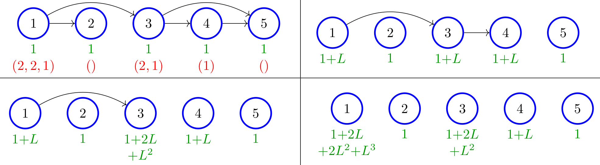
Figure 1: Exemplification of the constants occurring in Lemma 2.4. The red numbers indicate the number of outgoing paths of different lengths (e.g., $(2,1)$ below node 3 indicates that there are 2 paths of length 1, and 1 path of length 2 outgoing). The green numbers indicate how the constants for the cost change in the backward induction of the proof of Lemma 2.4. At the end of the backward induction (bottom right), the red numbers indicate the constants for each node, e.g., $2L+2L^{2}+L^{3}$ corresponds to $(2,2,1)$ for node 1.

Recall that $\hat{\mu}=\frac{1}{n}\sum_{i=1}^{n}\delta_{X^{i}}$ with $X^{1},\ldots,X^{n}$ being i.i.d. copies of $X\sim\mu$ is the standard empirical measure of $\mu$ with sample size $n$.

Lemma 2.5.

Let $k\leq K$, let $m\leq n$, and let $c_{\text{\rm pa}(k)}\in\mathcal{A}_{\text{\rm pa}(k)}$ with $\mu^{\mathcal{A}}(c_{\text{\rm pa}(k)})>0$. Then, conditionally on the event $n\cdot\hat{\mu}^{\mathcal{A}}(c_{\text{\rm pa}(k)})=m$, the random probability measure $\hat{\mu}^{\mathcal{A}}(\cdot\mid c_{\text{\rm pa}(k)})$ has the same distribution as the empirical measure of $\mu^{\mathcal{A}}(\cdot\mid c_{\text{\rm pa}(k)})$ with sample size $m$.

Proof.

Let $X\sim\mu$ and let $(X^{i})_{i=1}^{n}$ be an i.i.d. sample of $X$. For shorthand notation, set $(Y,Z):=(X_{\text{\rm pa}(k)},X_{k})$, similarity for $Y^{i}$ and $Z^{i}$. Moreover, write $c=c_{\text{\rm pa}(k)}$. Thus, by Lemma 2.3, $\mu^{\mathcal{A}}(c)=\mu(c)=\mathbb{P}(Y\in c)$ and by (2.1) for every measurable set $B\subset\mathcal{X}_{k}$, $\mu^{\mathcal{A}}(B\mid c)=\mathbb{P}(Z\in B\mid Y\in c)$.

Denote by $I$ the (random) set of indices $i\leq n$ for which $Y^{i}\in c$ so that $\hat{\mu}^{\mathcal{A}}(\cdot\mid c)=\frac{1}{|I|}\sum_{i\in I}\delta_{Z^{i}}$ by the definition of $\hat{\mu}^{\mathcal{A}}$. Thus, it suffices to show that, conditionally on $|I|=m$, the random vector $(Z^{i})_{i\in I}$ has the same distribution as an i.i.d. sample of size $m$ from $\mu^{\mathcal{A}}(dx_{k}\mid c)$; that is, $(Z^{i})_{i\in I}\sim(\mu^{\mathcal{A}}(dx_{k}\mid c))^{\otimes m}$. Equivalently, for a measurable set $B\subseteq(\mathcal{X}_{k})^{m}$ we need to show $\mathbb{P}((Z^{i})_{i\in I}\in B,|I|=m)=(\mu^{\mathcal{A}}(\cdot\mid c))^{\otimes m}(B)\,\cdot\,\mathbb{P}(|I|=m)$.

To that end, note that

$$\mathbb{P}\left((Z^{i})_{i\in I}\in B,\,|I|=m\right)$$

$$=\sum_{J\subset[n]\,:\,|J|=m}\mathbb{P}\left((Z^{i})_{i\in J}\in B,\,\forall i\in J:Y^{i}\in c,\,\forall i\notin J:Y^{i}\notin c\right)$$

$$=\sum_{J\subset[n]\,:\,|J|=m}\mathbb{P}\left((Z^{i})_{i\in J}\in B,\,\forall i\in J:Y^{i}\in c\right)\mathbb{P}\left(Y\notin c\right)^{n-m}$$ (2.6)

where we have used independence of the sample in the last equality. Since

$$\mathbb{P}\left((Z^{i})_{i\in J}\in B,\,\forall i\in J:Y^{i}\in{\rm c}\right)=(\mu(dx_{k}\mid c))^{\otimes m}(B)\mu(c)^{m}$$

and $\mu(dx_{k}\mid c)=\mu^{\mathcal{A}}(dx_{k}\mid c)$, the claim readily follows noting that there are $\binom{n}{m}$-many subsets $J$ in (2.6) and that $\binom{n}{m}\mu(c)^{m}(1-\mu(c))^{n-m}=\mathbb{P}\left(|I|=m\right)$. ∎

The final ingredient we require for the proof of Theorem 2.2 is on the speed of convergence of the classical empirical measure: if $\nu\in\mathcal{P}([0,1]^{r})$ and $\hat{\nu}$ denotes its empirical measure with sample size $n$, then

$$\mathbb{E}[\mathcal{W}(\nu,\hat{\nu})]\leq 8l_{n}(r)n^{-1/\max\{r,2\}},\qquad l_{n}(r)=\begin{cases}1&\text{if }r\neq 2,\\ \max\{\log(n),1\}&\text{if }r=2.\end{cases}$$ (2.7)

This is a standard result in probability theory; we refer to [15] for a version that quantifies the multiplicative constants explicitly.

2.2 Proof of Theorem 2.2

Step 1: It follows from Lemma 2.4 that

$$\mathcal{W}(\mu,\hat{\mu}^{\mathcal{A}}) \leq\sum_{k=1}^{K}M_{L,k}\int\mathcal{W}(\mu(\cdot\mid y_{\text{\rm pa}(k)}),\hat{\mu}^{\mathcal{A}}(\cdot\mid y_{\text{\rm pa}(k)}))\,\hat{\mu}^{\mathcal{A}}(dy_{\text{\rm pa}(k)}).$$

Moreover, for every $k\leq K$, since $\mu^{\mathcal{A}}(\cdot\mid y_{\text{\rm pa}(k)})$ is an average of measures of the form $\mu(\cdot\mid x_{\text{\rm pa}(k)})$ over $x_{\text{\rm pa}(k)}$ that satisfy $\|x_{\text{\rm pa}(k)}-y_{\text{\rm pa}(k)}\|\leq\delta_{\mathcal{A}}$, the triangle inequality together with Assumption 1.2 implies that

$$\mathcal{W}(\mu(\cdot\mid y_{\text{\rm pa}(k)}),\hat{\mu}^{\mathcal{A}}(\cdot\mid y_{\text{\rm pa}(k)}))\leq L\delta_{\mathcal{A}}+\mathcal{W}(\mu^{\mathcal{A}}(\cdot\mid y_{\text{\rm pa}(k)}),\hat{\mu}^{\mathcal{A}}(\cdot\mid y_{\text{\rm pa}(k)})).$$

Finally, since $\mu^{\mathcal{A}}(\cdot\mid y_{\text{\rm pa}(k)})$ and $\hat{\mu}^{\mathcal{A}}(\cdot\mid y_{\text{\rm pa}(k)})$ are constant in $y_{\text{\rm pa}(k)}$ as long $y_{\text{\rm pa}(k)}$ belongs to a fixed cell $c\in\mathcal{A}_{\text{\rm pa}(k)}$, since $\mu^{\mathcal{A}}(\cdot\mid c)=\mu(\cdot\mid c)$, we get

$$\mathcal{W}(\mu,\hat{\mu}^{\mathcal{A}}) \leq\sum_{k=1}^{K}M_{L,k}\left(L\delta_{\mathcal{A}}+\sum_{c\in\mathcal{A}_{\text{\rm pa}(k)}}\hat{\mu}^{\mathcal{A}}(c)\mathcal{W}(\mu^{\mathcal{A}}(\cdot\mid c),\hat{\mu}^{\mathcal{A}}(\cdot\mid c))\right).$$ (2.8)

Step 2: Fix $k\leq K$, and let $c\in\mathcal{A}_{\text{\rm pa}(k)}$. Observe that if $\mu^{\mathcal{A}}(c)=0$, then $\hat{\mu}^{\mathcal{A}}(c)=0$ almost surely. Otherwise, for $m\leq n$, by Lemma 2.5, conditionally on the event $n\hat{\mu}^{\mathcal{A}}(c)=m$, $\hat{\mu}^{\mathcal{A}}(\cdot\mid c)$ has the same distribution as the empirical measure of $\mu^{\mathcal{A}}(\cdot\mid c)$ with sample size $m$. Thus, setting $\bar{d}_{k}:=\max\{2,d_{k}\}$, it follows from (2.7) that

$$\mathbb{E}\left[\mathcal{W}(\mu^{\mathcal{A}}(\cdot\mid c)),\hat{\mu}^{\mathcal{A}}(\cdot\mid c))\mid n\hat{\mu}^{\mathcal{A}}(c)=m\right] \leq 8l_{m}(d_{k})m^{-1/\bar{d}_{k}}$$

$$\leq 8l_{n}(d_{k})\left(n\hat{\mu}^{\mathcal{A}}(c)\right)^{-1/\bar{d}_{k}}.$$

Therefore, by the tower property,

$$\mathbb{E}\left[\sum_{c\in\mathcal{A}_{\text{\rm pa}(k)}}\hat{\mu}^{\mathcal{A}}(c)\mathcal{W}(\mu^{\mathcal{A}}(\cdot\mid c),\hat{\mu}^{\mathcal{A}}(\cdot\mid c))\right]$$

$$=\sum_{c\in\mathcal{A}_{\text{\rm pa}(k)}}\mathbb{E}\left[\hat{\mu}^{\mathcal{A}}(c)\mathbb{E}\left[\mathcal{W}(\mu^{\mathcal{A}}(\cdot\mid c)),\hat{\mu}^{\mathcal{A}}(\cdot\mid c))\mid n\hat{\mu}^{\mathcal{A}}(c)\right]\right]$$

$$\leq\sum_{c\in\mathcal{A}_{\text{\rm pa}(k)}}\mathbb{E}\left[\hat{\mu}^{\mathcal{A}}(c)8l_{n}(d_{k})\left(n\hat{\mu}^{\mathcal{A}}(c)\right)^{-1/\bar{d}_{k}}\right]=:8\cdot l_{n}(d_{k})\cdot(1).$$

Moreover, by an application of Jensen’s inequality,

$$(1) =\frac{|\mathcal{A}_{\text{\rm pa}(k)}|}{n}\mathbb{E}\left[\frac{1}{|\mathcal{A}_{\text{\rm pa}(k)}|}\sum_{c\in\mathcal{A}_{\text{\rm pa}(k)}}\left(n\hat{\mu}^{\mathcal{A}}(c)\right)^{1-1/\bar{d}_{k}}\right]$$

$$\leq\frac{|\mathcal{A}_{\text{\rm pa}(k)}|}{n}\mathbb{E}\left[\left(\frac{1}{|\mathcal{A}_{\text{\rm pa}(k)}|}\sum_{c\in\mathcal{A}_{\text{\rm pa}(k)}}n\hat{\mu}^{\mathcal{A}}(c)\right)^{1-1/\bar{d}_{k}}\right]$$

$$=\frac{|\mathcal{A}_{\text{\rm pa}(k)}|}{n}\left(\frac{n}{|\mathcal{A}_{\text{\rm pa}(k)}|}\right)^{1-1/\bar{d}_{k}}=\left(\frac{n}{|\mathcal{A}_{\text{\rm pa}(k)}|}\right)^{-1/\bar{d}_{k}}.$$

Step 3: By combining Step 1 and Step 2,

$$\mathbb{E}\left[\mathcal{W}(\mu,\hat{\mu}^{\mathcal{A}})\right] \leq\sum_{k=1}^{K}M_{L,k}\left(L\delta_{\mathcal{A}}+8l_{n}(d_{k})\left(\frac{n}{|\mathcal{A}_{\text{\rm pa}(k)}|}\right)^{-1/\bar{d}_{k}}\right),$$ (2.9)

and it remains to estimate the last expression. By the choice of $\eta$ in the theorem, namely $\eta=\lfloor\frac{1}{d_{\rm loc}}\log_{2}(n)\rfloor$, we have that

$$\delta_{\mathcal{A}}=2^{-\eta}\leq 2^{-\frac{1}{d_{\rm loc}}\log_{2}(n)+1}=2n^{-1/d_{\rm loc}},$$

and

$$|\mathcal{A}_{\text{\rm pa}(k)}| =2^{\eta d_{\text{\rm pa}(k)}}\leq n^{d_{\text{\rm pa}(k)}/d_{\rm loc}}.$$

Therefore,

$$L\delta_{\mathcal{A}}+8l_{n}(d_{k})\left(\frac{n}{|\mathcal{A}_{\text{\rm pa}(k)}|}\right)^{-1/\bar{d}_{k}} \leq 2Ln^{-1/d_{\rm loc}}+8l_{n}(d_{k})\left(n^{1-d_{\text{\rm pa}(k)}/d_{\rm loc}}\right)^{-1/\bar{d}_{k}}$$

$$=:2Ln^{-1/d_{\rm loc}}+(2).$$

Finally, it remains to estimate the term $(2)$. If $d_{k}\neq 2$ then $l_{n}(d_{k})=1$ and, since $d_{\rm loc}\geq d_{\text{\rm pa}(k)}+\bar{d}_{k}$ by definition and thus $1-\frac{d_{\text{\rm pa}(k)}}{d_{\rm loc}}\geq\frac{\bar{d}_{k}}{d_{\rm loc}}$, we have $(2)\leq 8n^{-1/d_{\rm loc}}$. If $d_{k}=2$ and $d_{\rm loc}$ is not attained for this node, then $d_{\rm loc}\geq d_{\text{\rm pa}(k)}+\bar{d}_{k}+1$. Using that $\log(n)\leq rn^{1/r}$ for all $r,n\geq 1$, a straightforward calculation shows that $(2)\leq 16d_{\rm loc}n^{-1/d_{\rm loc}}$. Ultimately, if $d_{k}=2$ and $d_{\rm loc}$ is attained for this node, then clearly $(2)\leq 8l_{n}(d_{k})n^{-1/d_{\rm loc}}$. Hence the proof follows from (2.9). ∎

3 Sharp rates for graphical models with TV-Lipschitz kernels

This section contains the main results of this paper, namely we introduce an estimator $\hat{\mu}^{b\mathcal{A}}$ that achieves optimal error rates for graphical models. Before introducing the estimator, let us show that the assumption we impose in this section (Assumption 1.4) is implied by a classical assumption in density estimation:

Lemma 3.1.

Let $0<a<b$, $\mu\in\mathcal{P}_{G}(\mathcal{X})$ and assume that $\mu$ has a density w.r.t. the Lebesgue measure which is $D$-Lipschitz and takes values in the interval $[a,b]$. Then Assumption 1.4 is satisfied with $L=\frac{D}{a}+\frac{b}{a^{2}}$.

The proof of the lemma is given in Section 3.4. We shortly mention that the Lipschitz continuity and boundedness is not required globally—one may for instance check that restricting the assumption to a set $S=S_{1}\times\ldots\times S_{K}\subseteq\mathcal{X}$ with $\mu(S)=1$ suffices.

The estimator $\mu^{b\mathcal{A}}$ that will be shown to achieve the optimal rates is defined as follows. We recall that $\mu_{k}$ is the $k$-th marginal of $\mu$ and that for $c_{k}\subset\mathcal{X}_{k}$, $\mu_{k|c_{k}}$ is the restriction of $\mu_{k}$ to the set $c_{k}$ given by $\mu_{k|c_{k}}(A_{k})=\frac{\mu_{k}(A_{k}\cap c_{k})}{\mu_{k}(c_{k})}$ for Borel sets $A_{k}\subseteq\mathcal{X}_{k}$, which will only be relevant if $\mu_{k}(c_{k})>0$ (for completeness we may set $\mu_{k|c_{k}}$ to be the Dirac measure on the midpoint of the cell $c_{k}$ if $\mu_{k}(c_{k})=0$).

Definition 3.2.

Let $\mathcal{A}$ be the partition of $\mathcal{X}$ into cubes of side-length $\delta_{\mathcal{A}}=2^{-\eta}$. For $k=1,\dots,K$, we define

$$\mu^{b\mathcal{A}}(dx_{k}\mid x_{\text{\rm pa}(k)}):=\sum_{c_{k}\in\mathcal{A}_{k}}\mu\left(c_{k}\mid c_{\text{\rm pa}(k)}(x_{\text{\rm pa}(k)})\right)\cdot\mu_{k|c_{k}}(dx_{k})$$

and $\mu^{b\mathcal{A}}(dx)=\prod_{k=1}^{K}\mu^{b\mathcal{A}}(dx_{k}\mid x_{\text{\rm pa}(k)})$.

Under Assumption 1.1 and similarly to Lemma 2.3, $\mu^{b\mathcal{A}}$ is indeed well-defined (i.e., it is the same for all representatives of the disintegration of $\mu$), which follows from Lemma 3.4 below.

At this point, it perhaps makes sense to intuitively clarify the concept behind $\mu^{b\mathcal{A}}$ for the case $K=2$ and the graph $1\rightarrow 2$, in which case

$$\mu^{b\mathcal{A}}=\sum_{c_{1}\in\mathcal{A}_{1},c_{2}\in\mathcal{A}_{2}}\mu(c_{1}\times c_{2})\left(\mu_{1|c_{1}}\otimes\mu_{2|c_{2}}\right).$$ (3.1)

Thus, $\mu^{b\mathcal{A}}$ is locally a product measure, which on an intuitive level introduces additional smoothness (compared with $\mu^{\mathcal{A}}$). Supporting this fact, the superscript ‘$b\mathcal{A}$’ is intended to indicate that $\mu^{b\mathcal{A}}$ can in fact be obtained from $\mu$ by a twofold application of the operation $\mu\mapsto\mu^{\mathcal{A}}$—once forward along the topological ordering of the graph and once backwards; see Lemma 3.5 for the detailed statement of this fact and also Figure 2 for a visualization of $\mu^{b\mathcal{A}}$ in case that $\mu$ is a discrete measure.

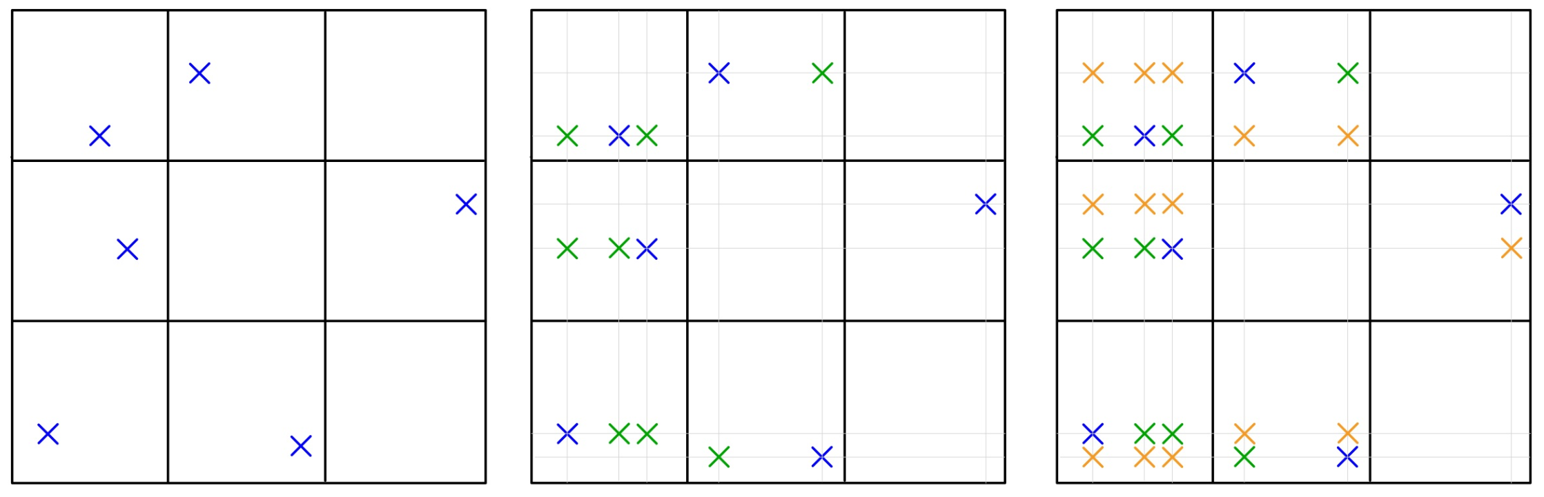
Figure 2: Visualization of estimators for a simple graph $1\rightarrow 2$ with $\mathcal{X}_{1}=\mathcal{X}_{2}=[0,1]$ with a partition of each interval into three subsets. We see the support of $\hat{\mu}$ (on the left), the support of $\hat{\mu}^{\mathcal{A}}$ (middle) and the support of $\hat{\mu}^{b\mathcal{A}}$ (right). Hereby, blue crosses are the initial data points, green are the new data points which are added by making the kernels constant in the direction from first to second coordinate, and orange are the new points which are added by further making the kernels constant in the direction from second to first coordinate. Eventually, on the right, we have product measures locally on each cube.

We are ready now to state the main result of this paper: For this, we recall $\bar{d}_{k}:=\max\{2,d_{k}\}$, $d_{\rm max}=\max_{k=1,\dots,K}\bar{d}_{k}$ and $d_{\rm loc}=\max_{k=1,\dots,K}\bar{d}_{k}+d_{\text{\rm pa}(k)}$.

Theorem 3.3.

Let $\mu\in\mathcal{P}_{G}(\mathcal{X})$ and suppose that Assumptions 1.1 and 1.4 hold. Set $\eta$ to be the largest integer satisfying $\eta\leq\frac{\log_{2}(n)}{2+d_{\rm loc}}$. Then,

$$\mathbb{E}\left[\mathcal{W}(\mu,\hat{\mu}^{b\mathcal{A}})\right]\leq C\cdot l_{n}\cdot\left(n^{-2/(2+d_{\rm loc})}+n^{-1/d_{\rm max}}\right),$$

where $C$ is a constant only depending on $L$, $G$, and $(d_{k})_{k=1}^{K}$, and where

$$l_{n}=\begin{cases}\max\{1,\log(n)\}&\text{if $n^{-2/(2+d_{\rm loc})}\geq n^{-1/d_{\rm max}}$ and $d_{\rm loc}$ is attained at $d_{k}=2$,}\\ \max\{1,\log(n)\}&\text{if $n^{-2/(2+d_{\rm loc})}\leq n^{-1/d_{\rm max}}$ and $\max_{k=1,\dots,K}d_{k}=2$,}\\ 1&\text{otherwise.}\end{cases}$$

In particular, if $d_{k}\geq 3$ for all $k$, then $l_{n}=1$.

3.1 Properties of $\mu^{b\mathcal{A}}$

Lemma 3.4.

Let $\mu\in\mathcal{P}(\mathcal{X})$, $2\leq k\leq K$ and $c_{\text{\rm pa}(k)}\in\mathcal{A}_{\text{\rm pa}(k)}$. Then, for all $c_{k}\in\mathcal{A}_{k}$,

$$\mu^{b\mathcal{A}}(c_{k}\mid c_{\text{\rm pa}(k)})=\mu(c_{k}\mid c_{\text{\rm pa}(k)}).$$

In particular, under Assumption 1.1, for any fully connected part of the graph $I\subseteq\{1,\dots,K\}$ and any cell $c_{I}\in\mathcal{A}_{I}$, we have $\mu^{b\mathcal{A}}(c_{I})=\mu(c_{I})$.

Proof.

By definition of $\mu^{b\mathcal{A}}$,

$$\mu^{b\mathcal{A}}(c_{k}\mid c_{\text{\rm pa}(k)})=\sum_{\tilde{c}_{k}\in\mathcal{A}_{k}}\mu(\tilde{c}_{k}\mid c_{\text{\rm pa}(k)})\cdot\mu_{k|\tilde{c}_{k}}(c_{k})=\mu(c_{k}\mid c_{\text{\rm pa}(k)})$$

since $\mu_{k|\tilde{c}_{k}}(c_{k})$ is equal to 1 if $c_{k}=\tilde{c_{k}}$ and zero otherwise.

The second part of the claim works inductively by showing the claim for sets $I\subseteq\{1,\dots,k\}$ for increasing $k$. For $k=1$ the statement is clearly true. Regarding the induction step from $k-1$ to $k$, we only need to show the claim for all fully connected parts $I\subseteq\{1,\dots,k\}$ with $k\in I$. For $J=\text{\rm pa}(k)\cup\{k\}$, by the assumption that $\text{\rm pa}(k)$ is fully connected, this follows by the above since

$$\mu^{b\mathcal{A}}(c_{J}) =\mu^{b\mathcal{A}}(c_{k}\times c_{\text{\rm pa}(k)})$$

$$=\mu^{b\mathcal{A}}(c_{\text{\rm pa}(k)})\mu^{b\mathcal{A}}(c_{k}\mid c_{\text{\rm pa}(k)})=\mu(c_{\text{\rm pa}(k)})\mu(c_{k}\mid c_{\text{\rm pa}(k)})=\mu(c_{J}).$$

For any other $I\subseteq\{1,\dots,k\}$ which is fully connected and with $k\in I$, we clearly have $I\subseteq J$ (otherwise an edge to $k$ must be missing), and hence

$$\mu^{b\mathcal{A}}(c_{I})=\sum_{c_{J\setminus I}}\mu^{b\mathcal{A}}(c_{I}\times c_{J\setminus I})=\sum_{c_{J\setminus I}}\mu(c_{I}\times c_{J\setminus I})=\mu(c_{I}).\qed$$

There is a subtle difference between $\mu^{\mathcal{A}}$ and $\mu^{b\mathcal{A}}$ (cf. Lemma 2.3 compared to Lemma 3.4). For the former, we had $\mu^{\mathcal{A}}(dx_{k}\mid c_{\text{\rm pa}(k)})=\mu(dx_{k}\mid c_{\text{\rm pa}(k)})$, while for the latter the equality holds only when restricted to cells in $\mathcal{X}_{k}$. This has several consequences—for instance, Lemma 2.5 no longer applies in this section and we need to suitably work around it, which is one of the objectives in Subsection 3.2 below.

The following clarifies the relation between $\mu^{\mathcal{A}}$ and $\mu^{b\mathcal{A}}$, which shows that the latter arises from a twofold (i.e., bidirectional) application of the $\mu^{\mathcal{A}}$ operation.

Lemma 3.5.

Let $K=2$ and define

$$\mathcal{S}\colon\mathcal{X}_{1}\times\mathcal{X}_{2}\to\mathcal{X}_{2}\times\mathcal{X}_{1},\quad(x_{1},x_{2})\mapsto(x_{2},x_{1}).$$

Then, for every $\mu\in\mathcal{P}(\mathcal{X})$,

$$\mu^{b\mathcal{A}}=\mathcal{S}\Big(\big(\mathcal{S}(\mu^{\mathcal{A}})\big)^{\mathcal{A}}\Big).$$

Proof.

Note that for $K=2$, there are only two relevant graph structures, $1\rightarrow 2$ and the graph without edges. For the graph without edges, the statement is clearly satisfied since $\mu^{b\mathcal{A}}=\mu^{\mathcal{A}}=\mu_{1}\otimes\mu_{2}$. We can thus restrict to the case $1\rightarrow 2$.

For notational simplicity, write $\mu=\nu\otimes R=\mathcal{S}(\theta\otimes V)$; in particular $\nu=\mu_{1}$ and $\theta=\mu_{2}$.

Step 1: We first claim that

$$\mathcal{S}((\nu\otimes R)^{\mathcal{A}})=\theta\otimes V^{r\mathcal{A}},$$ (3.2)

where

$$V^{r\mathcal{A}}(x_{2},dx_{1}) =\int H(\tilde{x}_{1},dx_{1})\,V(x_{2},d\tilde{x}_{1}),\qquad H(\tilde{x}_{1},dx_{1})=\sum_{\tilde{c}_{1}\in\mathcal{A}_{1}}\mathbf{1}_{\tilde{c}_{1}}(\tilde{x}_{1})\nu_{|\tilde{c}_{1}}(dx_{1}).$$

To show (3.2), it suffices to test it for Borel sets of the form $A\times B$ which satisfy $A\subseteq c_{1}$ and $B\subseteq c_{2}$ for some fixed $c_{1}\in\mathcal{A}_{1}$ and $c_{2}\in\mathcal{A}_{2}$. Denote by $R^{\mathcal{A}}$ the kernel of $\mu^{\mathcal{A}}$, that is, $\mu^{\mathcal{A}}=\nu\otimes R^{\mathcal{A}}$. Then, for $x_{1}\in A$, we have $R^{\mathcal{A}}(x_{1},B)=\int R(\tilde{x}_{1},B)\nu_{|c_{1}}(d\tilde{x}_{1})$ and thus

$$(\nu\otimes R)^{\mathcal{A}}(A\times B)=\nu(A)\int R(\tilde{x}_{1},B)\,\nu_{|c_{1}}(d\tilde{x}_{1}).$$ (3.3)

Moreover, since $H(\tilde{x}_{1},A)=\mathbf{1}_{A}(\tilde{x}_{1})\nu_{|c_{1}}(A)$ (in particular it is zero for $\tilde{x}_{1}\notin c_{1}$) and $\nu_{|c_{1}}(A)=\nu(A)/\nu(c_{1})$,

$$\theta\otimes V^{r\mathcal{A}}(B\times A) =\int_{B}\int H(\tilde{x}_{1},A)\,V(x_{2},d\tilde{x}_{1})\,\theta(dx_{2})$$

$$=\frac{\nu(A)}{\nu(c_{1})}\int_{B}V(x_{2},c_{1})\,\theta(dx_{2})$$

$$=\frac{\nu(A)}{\nu(c_{1})}\int_{c_{1}}R(x_{1},B)\,\nu(dx_{1})=\nu(A)\int R(x_{1},B)\,\nu_{|c_{1}}(dx_{1}).$$

This readily shows (3.2).

Step 2: Consider $A$ and $B$ as above. Note that by the definition of $\mathcal{S}$ and (3.2),

$$\mathcal{S}\Big(\big(\mathcal{S}((\nu\otimes R)^{\mathcal{A}}))^{\mathcal{A}}\Big)(A\times B)=(\theta\otimes V^{r\mathcal{A}})^{\mathcal{A}}(B\times A).$$

Moreover, by repeating the steps in (3.3) and using that $V^{r\mathcal{A}}(x_{2},A)=\nu|_{c_{1}}(A)V(x_{2},c_{1})$,

$$(\theta\otimes V^{r\mathcal{A}})^{\mathcal{A}}(B\times A) =\theta(B)\int V^{r\mathcal{A}}(x_{2},A)\,\theta_{|c_{2}}(dx_{2})$$

$$=\theta(B)\nu_{|c_{1}}(A)\int V(x_{2},c_{1})\,\theta_{|c_{2}}(dx_{2})$$

$$=\theta_{|c_{2}}(B)\nu_{|c_{1}}(A)(\theta\otimes V)(c_{2}\times c_{1}).$$

Finally, by (3.1), the last term is equal to $\mu^{b\mathcal{A}}(A\times B)$, which is exactly what we needed to show. ∎

The next ingredient to the proof of Theorem 3.3 is to show that the equality $\nu(c_{I})=\nu^{b\mathcal{A}}(c_{I})$ from Lemma 3.4 “almost” also holds for arbitrary cells $c\in\mathcal{A}$ under Assumption 1.4, we only require a small adjustment of order $\delta_{\mathcal{A}}^{2}$ (where $\delta_{\mathcal{A}}$ is, as always, the size of the cells in $\mathcal{A}$).

Before we proceed to state the result, let us spell out two observations that are important in what follows. Firstly, if $\nu\in\mathcal{P}_{G}(\mathcal{X})$, then by definition $\nu(dx_{k}\mid x_{1:k-1})=\nu(dx_{k}\mid x_{\text{\rm pa}(k)})$. This relation is no longer true for sets, e.g., it is no longer true that $\nu(c_{k}\mid c_{1:k-1})$ is equal to $\nu(c_{k}\mid c_{\text{\rm pa}(k)})$ for cells $c\in\mathcal{A}$. However, if $\nu(c_{k}|x_{\text{\rm pa}(k)})$ is constant for $x_{\text{\rm pa}(k)}\in c_{\text{\rm pa}(k)}$, then it is true. In particular, we have that

$$\mu^{b\mathcal{A}}(c_{k}\mid c_{1:k-1})=\mu^{b\mathcal{A}}(c_{k}\mid c_{\text{\rm pa}(k)})$$ (3.4)

for all cells $c\in\mathcal{A}$ and $k=1,\dots,K$.

In the formulation of the next result we will use signed measures and denote by $\|\nu\|_{{\rm TV}}={\rm TV}(\nu,0)=\sup_{f:|f|\leq 1/2}\int f\,d\nu$ the total variation norm of a signed measure $\nu$.

Lemma 3.6.

Let Assumptions 1.1 and 1.4 hold. Then there exist a constant $C$ that only depends on $G$ and $L$ and a signed measure $\tilde{\mu}$ which satisfies $\|\tilde{\mu}\|_{{\rm TV}}\leq C\delta^{2}$, such that

$$\mu(c)=\mu^{b\mathcal{A}}(c)+\tilde{\mu}(c)~~\text{ for all }c\in\mathcal{A}.$$

Proof.

We inductively show the corresponding statement for $\mu_{1:k}$ and $\mu^{b\mathcal{A}}_{1:k}$. The start $k=1$ is trivial since $\mu_{1}=\mu^{b\mathcal{A}}_{1}$; hence we may choose $\tilde{\mu}_{1}=0$. The proof for the induction from $k-1$ to $k$ requires some preparations, spelled out in the next step.

Step 0: We split the nodes

$$\{1,\dots,k\}=\text{\rm pre}(k)\cup\text{\rm pa}(k)\cup\{k\}$$

into $k$, its parents, and the rest. Moreover, we disintegrate $\mu_{1:k}$ via $\text{\rm pa}(k)$, thus

$$\mu_{1:k}(dx_{1:k})=\mu_{\text{\rm pa}(k)}(dx_{\text{\rm pa}(k)})\,\mu(dx_{k}\mid x_{\text{\rm pa}(k)})\,\mu(dx_{\text{\rm pre}(k)}\mid x_{\text{\rm pa}(k)}).$$

Note that this disintegration holds true since $\mu\in\mathcal{P}_{G}$, which means the variable $k$ and the variables in $\text{\rm pre}(k)$ are conditionally independent given the $\text{\rm pa}(k)$ variables.

To simplify notation, we shall assume that $k=3$, $\text{\rm pa}(k)=2$, $\text{\rm pre}(k)=1$, and write $R_{2\to 3}(x_{2},dx_{3})=\mu(dx_{3}\mid x_{2})$ and similarly $R_{2\to 1}$; thus

$$\mu(dx_{1:3})=\mu_{3}(dx_{2})R_{2\to 3}(x_{2},dx_{3})R_{2\to 1}(x_{2},dx_{1}).$$

This can be done without loss of generality and the proof in the original case follows simply by exchanging notation.

Step 1: Define the averaged version of $R_{2\to 3}$ via

$$\bar{R}_{2\to 3}(x_{2},dx_{3}) :=\int R_{2\to 3}(\tilde{x}_{2},dx_{3})\,\mu_{2}|_{c_{2}(x_{2})}(d\tilde{x}_{2})$$

for $x_{2}\in\mathcal{X}_{2}$. Thus $x_{2}\mapsto\bar{R}_{2\to 3}(x_{2},dx_{3})$ is constant as long as $x_{2}$ belongs to a fixed cell $c_{2}$, and we often write $\bar{R}_{2\to 3}(c_{2},dx_{3})$ in that case. By the convexity of ${\rm TV}$, we have that ${\rm TV}(\bar{R}_{2\to 3}(x_{2},\cdot),R_{2\to 3}(x_{2},\cdot))\leq L\delta_{\mathcal{A}}$ and hence

$$R_{2\to 3}(x_{2},dx_{3})=\bar{R}_{2\to 3}(x_{2},dx_{3})+\delta_{\mathcal{A}}D_{2\to 3}(x_{2},dx_{3})$$

for some kernel $D_{2\to 3}$ that satisfies $\|D_{2\to 3}(x_{2},dx_{3})\|_{{\rm TV}}\leq L$. Moreover, by definition we find $\int_{c_{2}}D_{2\to 3}(x_{2},dx_{3})\,\mu(dx_{2})=0$ for every $c_{2}\in\mathcal{A}_{2}$.

Step 2: Here we analyse the error made by replacing $R_{2\to 3}$ by $\bar{R}_{2\to 3}$. Fix $c_{1:3}\in\mathcal{A}_{1:3}$ Using the decomposition $R_{2\to 3}=\bar{R}_{2\to 3}+\delta_{\mathcal{A}}D_{2\to 3}$ and that $\bar{R}_{2\to 3}(x_{2},\cdot)$ is constant for $x_{2}\in c_{2}$,

$$\begin{split}\mu(c_{1:3})&=\int_{c_{1:2}}\left(\bar{R}_{2\to 3}(x_{2},c_{3})+\delta_{\mathcal{A}}D_{2\to 3}(x_{2},c_{3})\right)\,\mu_{1:2}(dx_{1:2})\\ &=\mu_{1:2}(c_{1:2})\bar{R}_{2\to 3}(c_{2},c_{3})+\delta_{\mathcal{A}}\int_{c_{1:2}}D_{2\to 3}(x_{2},c_{3})\,\mu_{1:2}(dx_{1:2})\\ &=(1)+(2).\end{split}$$ (3.5)

By the induction hypothesis,

$$\begin{split}(1)&=\left(\mu_{1:2}^{b\mathcal{A}}(c_{1:2})+\tilde{\mu}_{1:2}(c_{1:2})\right)\bar{R}_{2\to 3}(c_{2},c_{3})\\ &=\mu_{1:3}^{b\mathcal{A}}(c_{1:3})+\tilde{\mu}_{1:2}(c_{1:2})\bar{R}_{2\to 3}(c_{2},c_{3}).\end{split}$$ (3.6)

(For the second equality note that while $\mu_{1:2}^{b\mathcal{A}}(c_{1:2})\bar{R}_{2\to 3}(c_{2},c_{3})=\mu_{1:3}^{b\mathcal{A}}(c_{1:3})$ does not hold for arbitrary sets $c_{1:3}\subset\mathcal{X}_{1:3}$, it does hold for cells.)

Step 3: We proceed to control the term $(2)$. Analogously to Step 1, define $\bar{R}_{2\to 1}(x_{2},dx_{1})=\int R_{2\to 1}(\tilde{x}_{2},dx_{1})\,\mu_{2}|_{c_{2}(x_{2})}(d\tilde{x}_{2})$ and $D_{2\to 1}$ via $R_{2\to 1}=\bar{R}_{2\to 1}+\delta_{\mathcal{A}}D_{2\to 1}$. Using this notation, we can write

$$\begin{split}(2)&=\delta_{\mathcal{A}}\int_{c_{2}}D_{2\to 3}(x_{2},c_{3})\bar{R}_{2\to 1}(x_{2},c_{1})\,\mu_{2}(dx_{2})\\ &\quad+\delta_{\mathcal{A}}^{2}\int_{c_{2}}D_{2\to 3}(x_{2},c_{3})D_{2\to 1}(x_{2},dx_{1})\,\mu_{2}(dx_{2})\\ &=(3)+(4).\end{split}$$ (3.7)

Since $\bar{R}_{2\to 1}(x_{2},c_{1})$ is constant for $x_{2}\in c_{2}$ and $\int_{c_{2}}D_{2\to 3}(x_{2},c_{3})\,\mu_{2}(dx_{2})=0$ by the definition of $D_{2\to 3}$, it follows that

$$\begin{split}(3)&=\delta_{\mathcal{A}}\int_{c_{2}}D_{2\to 3}(x_{2},c_{3})\,\mu_{2}(dx_{2})\,\bar{R}_{2\to 1}(c_{2},c_{1})=0.\end{split}$$ (3.8)

Step 4: Define the (signed) measure

$$\tilde{\mu}_{1:k}=\tilde{\mu}_{1:2}\otimes\bar{R}_{2\to 3}+\delta_{\mathcal{A}}^{2}\cdot\mu_{2}\otimes D_{2\to 3}\otimes D_{2\to 1}.$$

One readily checks that $\|\tilde{\mu}_{1:k}\|_{{\rm TV}}\leq\|\tilde{\mu}_{1:3}\|_{{\rm TV}}+(\delta_{\mathcal{A}}L)^{2}$. By (3.5)–(3.8) we have that $\mu^{b\mathcal{A}}(c_{1:4})=\mu(c_{1:4})+\tilde{\mu}(c_{1:4})$, which completes the induction step and thus the proof. ∎

To eventually bound $\mathcal{W}(\mu,\mu^{b\mathcal{A}})$, we first show how to control ${\rm TV}(\mu,\mu^{b\mathcal{A}})$.

Lemma 3.7.

Let $K=2$ and assume that $\mu$ satisfies Assumption 1.4. Then,

$${\rm TV}(\mu,\mu^{b\mathcal{A}}) \leq 2L\delta_{\mathcal{A}},$$ (3.9)

$$\int{\rm TV}(\mu(dx_{2}\mid x_{1}),\mu^{b\mathcal{A}}(dx_{2}\mid x_{1}))\,\mu(dx_{1}) \leq 2L\delta_{\mathcal{A}}.$$ (3.10)

Proof.

Write

$${\rm TV}(\mu,\mu^{b\mathcal{A}})\leq{\rm TV}(\mu,\mu^{\mathcal{A}})+{\rm TV}(\mu^{\mathcal{A}},\mu^{b\mathcal{A}}).$$

To estimate ${\rm TV}(\mu,\mu^{\mathcal{A}})$, since $\mu^{\mathcal{A}}(dx_{2}\mid x_{1})$ is the average of $\mu(dx_{2}\mid\tilde{x}_{1})$ over $\tilde{x}_{1}$ that satisfy $\|x_{1}-\tilde{x}_{1}\|\leq\delta_{\mathcal{A}}$, it follows from convexity of the total variation distance that

$${\rm TV}(\mu(dx_{2}\mid x_{1}),\mu^{\mathcal{A}}(dx_{2}\mid x_{1}))\leq L\delta_{\mathcal{A}}.$$

And since $\mu$ and $\mu^{\mathcal{A}}$ have the same marginals,

$${\rm TV}(\mu,\mu^{\mathcal{A}})=\int{\rm TV}(\mu(dx_{2}\mid x_{1}),\mu^{\mathcal{A}}(dx_{2}\mid x_{1}))\,\mu_{1}(dx_{1})\leq L\delta_{\mathcal{A}}.$$ (3.11)

To estimate ${\rm TV}(\mu^{\mathcal{A}},\mu^{b\mathcal{A}})$, we recall from Lemma 3.5 that

$$\mu^{b\mathcal{A}}=\mathcal{S}\Big(\big(\mathcal{S}(\mu^{\mathcal{A}})\big)^{\mathcal{A}}\Big)$$

and (recalling the proof of Lemma 3.5) that

$$\mu^{\mathcal{A}}=\mu_{2}(dx_{2})V^{r\mathcal{A}}(x_{2},dx_{1})$$

where $V^{r\mathcal{A}}(x_{2},dx_{1})=\int H(\tilde{x}_{1},dx_{1})\,\mu(d\tilde{x}_{1}\mid x_{2})$. The exact form of $H$ is not important, only that $H$ is a stochastic kernel (i.e., it has total variation norm 1 for each $\tilde{x}_{1}$), hence $x_{2}\mapsto V^{r\mathcal{A}}(x_{2},dx_{1})$ is $L$-Lipschitz in total variation. Since the operator $\mathcal{S}^{-1}$ does not change the total variation distance,

$${\rm TV}\left(\mu^{\mathcal{A}},\mu^{b\mathcal{A}}\right)={\rm TV}\left(\mu^{\mathcal{A}},\mathcal{S}(\mathcal{S}(\mu^{\mathcal{A}})^{\mathcal{A}})\right)={\rm TV}\left(\mathcal{S}(\mu^{\mathcal{A}}),\mathcal{S}(\mu^{\mathcal{A}})^{\mathcal{A}}\right).$$

Thus, the same arguments as used when estimating ${\rm TV}(\mu,\mu^{\mathcal{A}})$ show that ${\rm TV}(\mu^{\mathcal{A}},\mu^{b\mathcal{A}})\leq L\delta_{\mathcal{A}}$. This completes the proof of (3.9). Finally (3.10) follows because $\mu$ and $\mu^{b\mathcal{A}}$ have the same marginals. ∎

In the proof of Theorem 3.3 we shall make use of the Kantorovich–Rubinstein duality, that is, for any $\nu,\tilde{\nu}\in\mathcal{P}(\mathcal{X})$,

$$\mathcal{W}(\nu,\tilde{\nu})=\sup_{f\in\mathcal{F}}\int f\,d(\nu-\tilde{\nu}),$$ (3.12)

where $\mathcal{F}$ is the set of all functions from $(\mathcal{X},\|\cdot\|)$ to $\mathbb{R}$ that are $1$-Lipschitz (and satisfy $f(0)=0$). See, e.g., [43, Theorem 5.10 & 5.16] for a proof of this fact.

The following gives the main result on controlling the bias $W(\mu,\mu^{b\mathcal{A}})$ for Theorem 3.3.

Lemma 3.8.

Let $\mu\in\mathcal{P}_{G}(\mathcal{X})$ and suppose Assumptions 1.1 and 1.4 hold. Then,

$${\rm TV}(\mu,\mu^{b\mathcal{A}}) \leq(K-1)2L\delta_{\mathcal{A}},$$

$$\mathcal{W}(\mu,\mu^{b\mathcal{A}}) \leq((K-1)2L+2C)\delta_{\mathcal{A}}^{2},$$

where $C$ is the constant from Lemma 3.6.

Proof.

The first inequality follows by using the optimal transport definition of the total variation distance and iterating (3.10). Indeed, we claim that for every $M=1,\dots,K$,

$${\rm TV}\left(\mu_{1:M},\mu^{b\mathcal{A}}_{1:M}\right)\leq(M-1)2L\delta_{\mathcal{A}}.$$

The proof of this claim is via induction, noting that the case $M=2$ is already covered by Lemma 3.7. For the induction step from $M-1$ to $M$, let $\pi$ be an optimal coupling for the OT-representation of ${\rm TV}(\mu_{1:M-1},\mu^{b\mathcal{A}}_{1:M-1})$. Thus

$$\pi(\{x_{1:M-1},y_{1:M-1}:x_{1:M-1}\neq y_{1:M-1}\})\leq(M-2)2L\delta_{\mathcal{A}}.$$

Similarly as in the proof of Lemma 2.4, let $\pi^{x_{\text{\rm pa}(M)},y_{\text{\rm pa}(M)}}$ be a measurable family of couplings between $\mu(dx_{M}|x_{\text{\rm pa}(M)})$ and $\mu^{b\mathcal{A}}(dy_{M}|y_{\text{\rm pa}(M)})$ which are optimal for their ${\rm TV}$-distance; and let $\Gamma$ be the concatenation with respect to $\pi$. Thus

$$\Gamma(\{x_{1:M},y_{1:M}:x_{1:M}\neq y_{1:M}\})$$

$$\leq(M-2)2L\delta_{\mathcal{A}}+\int\pi^{x_{\text{\rm pa}(M)},x_{\text{\rm pa}(M)}}(\{x_{M},y_{M}:x_{M}\neq y_{M}\})\,\mu(dx_{1:M-1})$$

$$=(M-2)2L\delta_{\mathcal{A}}+\int{\rm TV}\left(\mu(dx_{M}|x_{\text{\rm pa}(M)}),\mu^{b\mathcal{A}}(dx_{M}|x_{\text{\rm pa}(M)})\right)\,\mu(dx_{1:M-1})$$

$$\leq(M-2)2L\delta_{\mathcal{A}}+2L\delta_{\mathcal{A}},$$

where we used the induction hypothesis in the first inequality, and (3.10) in the second one inequality. This completes the proof of the claim, and thus of the first statement in the lemma.

For the proof of the second statement we rely on the Kantorovich-Rubinstein duality, see (3.12). Let $f$ be $1$-Lipschitz with $f(0)=0$. Denoting by $m_{c}$ the midpoint of a cell $c\in\mathcal{A}$, we have that

$$\int f\,d(\mu-\mu^{b\mathcal{A}}) =\sum_{c\in\mathcal{A}}\int_{c}f(x)-f(m_{c})\,d(\mu-\mu^{b\mathcal{A}})+\sum_{c\in\mathcal{A}}f(m_{c})\,(\mu(c)-\mu^{b\mathcal{A}}(c))$$

$$=:(1)+(2).$$

Since $|f(x)-f(m_{c})|\leq\delta_{\mathcal{A}}/2$ for every $c\in\mathcal{A}$ and every $x\in c$, by the first part of the lemma,

$$(1)\leq\sum_{c\in\mathcal{A}}\frac{\delta_{\mathcal{A}}}{2}\,|\mu(c)-\mu^{b\mathcal{A}}(c)|\leq\delta_{\mathcal{A}}\,\|\mu-\mu^{b\mathcal{A}}\|_{\mathrm{TV}}\leq(K-1)2L\delta_{\mathcal{A}}^{2}.$$

Moreover, using the notation of Lemma 3.6, and that $|f(m_{c})|\leq 1$ for every $c\in\mathcal{A}$,

$$(2)=\sum_{c\in\mathcal{A}}f(m_{c})\,\tilde{\mu}(c)\leq 2\|\tilde{\mu}\|_{\mathrm{TV}}\leq 2C\delta_{\mathcal{A}}^{2}.$$

As $f$ was arbitrary, this shows that $\mathcal{W}(\mu,\mu^{b\mathcal{A}})\leq((K-1)2L+2C)\delta_{\mathcal{A}}^{2}$, as claimed. ∎

3.2 Projection to fully discrete measures

The next preliminary results needed for the proof of Theorem 3.3 requires projecting and working on the midpoints $\mathcal{M}$ of the cells $\mathcal{A}$.

Define $\mu^{\mathcal{M}}$ by

$$\mu^{\mathcal{M}}(\{x\}):=\mu^{b\mathcal{A}}(c(x)),\qquad x\in\mathcal{M}.$$

Note that $\mu^{\mathcal{M}}_{1}(\{x_{1}\})=\mu^{b\mathcal{A}}(c_{1}(x_{1}))$ for every $x_{1}\in\mathcal{M}_{1}$. Moreover, by (3.4), we have that $\mu^{\mathcal{M}}\in\mathcal{P}_{G}(\mathcal{X})$, and by Lemma 3.4, that for every $k=2,\dots,K$ and $x_{\text{\rm pa}(k)}\in\mathcal{M}_{\text{\rm pa}(k)}$,

$$\mu^{\mathcal{M}}(\{x_{k}\}\mid x_{\text{\rm pa}(k)}) =\mu^{b\mathcal{A}}(c_{k}(x_{k})\mid x_{\text{\rm pa}(k)})=\mu(c_{k}(x_{k})\mid c_{\text{\rm pa}(k)}(x_{\text{\rm pa}(k)})).$$ (3.13)

Moreover, we have the following:

Lemma 3.9.

The kernels of $\mu^{\mathcal{M}}$ are $(2L+1)$-Lipschitz w.r.t. $\mathcal{W}$; that is, for every $2\leq k\leq K$ and $x_{\text{\rm pa}(k)},\tilde{x}_{\text{\rm pa}(k)}\in\mathcal{M}_{\text{\rm pa}(k)}$,

$$\mathcal{W}\left(\mu^{\mathcal{M}}(dx_{k}\mid x_{\text{\rm pa}(k)}),\mu^{\mathcal{M}}(dx_{k}\mid\tilde{x}_{\text{\rm pa}(k)})\right)\leq(2L+1)\|x_{\text{\rm pa}(k)}-\tilde{x}_{\text{\rm pa}(k)}\|.$$

Proof.

We first claim that, for every $x_{\text{\rm pa}(k)},\tilde{x}_{\text{\rm pa}(k)}\in\mathcal{M}_{\text{\rm pa}(k)}$,

$$\begin{split}&\mathcal{W}\left(\mu(dx_{k}\mid c_{\text{\rm pa}(k)}(x_{\text{\rm pa}(k)})),\mu(dx_{k}\mid c_{\text{\rm pa}(k)}(\tilde{x}_{\text{\rm pa}(k)}))\right)\\ &\quad\leq 2L\|x_{\text{\rm pa}(k)}-\tilde{x}_{\text{\rm pa}(k)}\|.\end{split}$$ (3.14)

To that end, first note that for every distinct $x_{\text{\rm pa}(k)},\tilde{x}_{\text{\rm pa}(k)}\in\mathcal{M}_{\text{\rm pa}(k)}$ and $x_{\text{\rm pa}(k)}^{\prime}\in c_{\text{\rm pa}(k)}(x_{\text{\rm pa}(k)})$ and $\tilde{x}_{\text{\rm pa}(k)}^{\prime}\in c_{k}(\tilde{x}_{\text{\rm pa}(k)})$,

$$\|x_{\text{\rm pa}(k)}^{\prime}-\tilde{x}_{\text{\rm pa}(k)}^{\prime}\|\leq 2\|x_{\text{\rm pa}(k)}-\tilde{x}_{\text{\rm pa}(k)}\|.$$

Moreover, since $\mu(dx_{k}\mid c_{\text{\rm pa}(k)}(x_{\text{\rm pa}(k)}))$ is the average of $\mu(dx_{k}\mid x^{\prime}_{\text{\rm pa}(k)})$ over $x_{\text{\rm pa}(k)}^{\prime}\in c_{\text{\rm pa}(k)}(x_{\text{\rm pa}(k)})$ and similarly for $\mu(dx_{k}\mid\tilde{x}^{\prime}_{\text{\rm pa}(k)})$, a twofold application of convexity of $\mathcal{W}$ shows that

$$\mathcal{W}\left(\mu(dx_{k}\mid c_{\text{\rm pa}(k)}(x_{\text{\rm pa}(k)})),\mu(dx_{k}\mid c_{\text{\rm pa}(k)}(\tilde{x}_{\text{\rm pa}(k)})\right)$$

$$\quad\leq L\max_{x_{\text{\rm pa}(k)}^{\prime}\in c(x_{\text{\rm pa}(k)}),\tilde{x}_{\text{\rm pa}(k)}^{\prime}\in c(\tilde{x}_{\text{\rm pa}(k)})}\|x_{\text{\rm pa}(k)}^{\prime}-\tilde{x}_{\text{\rm pa}(k)}^{\prime}\|\leq 2L\|x_{\text{\rm pa}(k)}-\tilde{x}_{\text{\rm pa}(k)}\|$$

for all $x_{\text{\rm pa}(k)},\tilde{x}_{\text{\rm pa}(k)}\in\mathcal{M}_{\text{\rm pa}(k)}$. This shows (3.14).

In the next step, denote by $\psi\colon\mathcal{X}_{k}\to\mathcal{M}_{k}$ the map projecting cells to their centres, so that by (3.13),

$$\mu^{\mathcal{M}}(dx_{k}\mid x_{\text{\rm pa}(k)})=\psi\left(\mu(dx_{k}\mid c_{\text{\rm pa}(k)}(x_{\text{\rm pa}(k)}))\right).$$

Since $\|\psi(x_{k})-x_{k}\|\leq\delta_{\mathcal{A}}/2$, we have

$$\|\psi(x_{k})-\psi(\tilde{x}_{k})\|\leq\|x_{k}-\tilde{x}_{k}\|+\delta_{\mathcal{A}}$$

for all $x_{k},\tilde{x}_{k}\in\mathcal{X}_{k}$, and thus a basic coupling argument shows that

$$\mathcal{W}\left(\mu^{\mathcal{M}}(dx_{k}\mid x_{\text{\rm pa}(k)}),\mu^{\mathcal{M}}(dx_{k}\mid\tilde{x}_{\text{\rm pa}(k)})\right)$$

$$\quad\leq\mathcal{W}\left(\mu(dx_{k}\mid c_{\text{\rm pa}(k)}(x_{\text{\rm pa}(k)})),\mu(dx_{k}\mid c_{\text{\rm pa}(k)}(\tilde{x}_{\text{\rm pa}(k)}))\right)+\delta_{\mathcal{A}}$$

$$\quad\leq 2L\|x_{\text{\rm pa}(k)}-\tilde{x}_{\text{\rm pa}(k)}\|+\delta_{\mathcal{A}}$$

where we have used (3.14) in the last inequality. Since, for every distinct $x_{\text{\rm pa}(k)},\tilde{x}_{\text{\rm pa}(k)}\in\mathcal{M}_{k}$ we have that $\|x_{\text{\rm pa}(k)}-\tilde{x}_{\text{\rm pa}(k)}\|\geq\delta_{\mathcal{A}}$, the claim follows. ∎

Lemma 3.10.

Let $1\leq k\leq K$, set $\nu\in\mathcal{P}(\mathcal{X}_{k})$ to be a probability measure which is supported on $\mathcal{M}_{k}$, and denote by $\hat{\nu}$ its empirical measures with $m$ samples. Recall that $2^{-\eta}$ is the side-length of the cells. Then, we have

$$\mathbb{E}\left[\mathcal{W}(\nu,\hat{\nu})\right]\leq\begin{cases}5m^{-1/2},&\text{if }d_{k}=1,\\ 2\eta m^{-1/2},&\text{if }d_{k}=2,\\ 8m^{-1/2}2^{\eta\cdot(\frac{d_{k}}{2}-1)},&\text{if }d_{k}\geq 3.\end{cases}$$

Proof.

For $\ell=1,\dots,\eta$, denote by $\mathcal{A}_{k}(\ell)$ the partition of $\mathcal{X}_{k}$ into cells of side-lengths $2^{-\ell}$. Thus $|\mathcal{A}_{k}(\ell)|=2^{\ell d_{k}}$ and $\mathcal{A}_{k}(\eta)=\mathcal{A}_{k}$, and $\mathcal{M}_{k}$ are the mid-points of the cells in $\mathcal{A}_{k}$. The standard refinement-of-partition chaining argument from Dudley [12] yields that

$$\mathbb{E}\left[\mathcal{W}(\nu,\hat{\nu})\right]\leq\sum_{\ell=1}^{\eta}2^{1-\ell}\left(\frac{|\mathcal{A}_{k}(\ell)|}{m}\right)^{1/2}=2m^{-1/2}\sum_{\ell=1}^{\eta}2^{\ell\cdot(\frac{d_{k}}{2}-1)}.$$

The wanted estimate on $\mathbb{E}[\mathcal{W}(\nu,\hat{\nu})]$ in the case $d_{k}=2$ now follows immediately. The cases $d_{k}=1$ and $d_{k}\geq 3$ follow by computing the geometric series. ∎

Lemma 3.11.

Let $1\leq k\leq K$, fix $x_{\text{\rm pa}(k)}\in\mathcal{M}_{\text{\rm pa}(k)}$ and let $c_{\text{\rm pa}(k)}$ be the unique cell containing $x_{\text{\rm pa}(k)}$. Then, conditionally on the event $n\cdot\hat{\mu}^{\mathcal{M}}(\{x_{\text{\rm pa}(k)}\})=m$, the random probability measure $\hat{\mu}^{\mathcal{M}}(dx_{k}|x_{\text{\rm pa}(k)})$ has the same distribution as the empirical measure of $\mu^{\mathcal{M}}(dx_{k}|x_{\text{\rm pa}(k)})$ with sample size $m$.

Proof.

Let $X\sim\mu$ and let $(X^{i})_{i=1}^{n}$ the i.i.d. sample selected according to $\mu$. Set $I$ to be the random set of indices $1\leq i\leq n$ for which $X^{i}_{\text{\rm pa}(k)}\in c_{\text{\rm pa}(k)}$; thus $n\cdot\hat{\mu}^{\mathcal{M}}(c_{\text{\rm pa}(k)})=|I|$ (by Lemma 3.4).

First note that, conditionally on $|I|=m$, the vector $(X^{i}_{k})_{i\in I}$ has the same distribution as that of an i.i.d. sample of the distribution $\mu(dx_{k}\mid c_{\text{\rm pa}(k)})$ (this follows exactly as in the proof of Lemma 2.5). In particular, conditionally on $|I|=m$, $\alpha:=\frac{1}{|I|}\sum_{i\in I}\delta_{X^{i}_{k}}$ has the same distribution as the empirical measure of $\mu(dx_{k}\mid c_{\text{\rm pa}(k)})$ with sample size $m$.

Next, denote by $\psi\colon\mathcal{X}_{k}\to\mathcal{M}_{k}$ the projection of each cell to its center. Thus $\mu^{\mathcal{M}}(dx_{k}\mid x_{\text{\rm pa}(k)})$ is the push-forward of $\mu(dx_{k}\mid c_{\text{\rm pa}(k)})$ under $\psi$ and, similarly, $\hat{\mu}^{\mathcal{M}}(dx_{k}\mid c_{\text{\rm pa}(k)})$ is the push-forward of $\alpha$ under $\psi$. Since the push-forward of the empirical measure is the empirical measure of the push-forward of the measure, the claim follows. ∎

Lemma 3.12.

There is a constant $C$ depending only on $G$ and $L$ for which

$$\mathcal{W}(\mu^{\mathcal{M}},\hat{\mu}^{\mathcal{M}})\leq C\cdot n^{-1/2}\cdot\begin{cases}\delta_{\mathcal{A}}^{1-d_{\rm loc}/2}&\text{if }d_{\rm loc}\text{ is not attained at }d_{k}=2,\\ \log(\frac{1}{\delta_{\mathcal{A}}})\delta_{\mathcal{A}}^{1-d_{\rm loc}/2}&\text{else}.\end{cases}$$

Proof.

By Lemma 3.9, the kernels of $\mu^{\mathcal{M}}$ are $2L+1$-Lipschitz w.r.t. the Wasserstein distance. Hence, it follows from Lemma 2.4 (noting that Lipschitz continuity of the kernels of $\mu^{\mathcal{M}}$ only needs to hold $\mu^{\mathcal{M}}$-almost surely) that

$$\mathcal{W}\left(\mu^{\mathcal{M}},\hat{\mu}^{\mathcal{M}}\right) \leq C\sum_{k=1}^{K}\int\mathcal{W}\left(\mu^{\mathcal{M}}(dx_{k}\mid x_{\text{\rm pa}(k)}),\hat{\mu}^{\mathcal{M}}(dx_{k}\mid x_{\text{\rm pa}(k)})\right)\,\hat{\mu}^{\mathcal{M}}(dx).$$

To proceed further, we fix $k$ and distinguish between the cases $d_{k}\in\{1,2\}$ and $d_{k}\geq 3$, starting with the latter. An application of Lemma 3.11 together with Lemma 3.10 shows that

$$\mathbb{E}\left[\mathcal{W}\left(\mu^{\mathcal{M}}(dx_{k}\mid x_{\text{\rm pa}(k)}),\hat{\mu}^{\mathcal{M}}(dx_{k}\mid x_{\text{\rm pa}(k)})\right)\mid\hat{\mu}^{\mathcal{M}}(\{x_{\text{\rm pa}(k)}\})\right]\leq\frac{8\cdot 2^{\eta(d_{k}/2-1)}}{(n\cdot\hat{\mu}^{\mathcal{M}}(\{x_{\text{\rm pa}(k)}\}))^{1/2}}.$$

Therefore, it follows from Jensen’s inequality exactly as in the proof of Theorem 2.2 that

$$(1) :=\mathbb{E}\left[\int\mathcal{W}\left(\mu^{\mathcal{M}}(dx_{k}\mid x_{\text{\rm pa}(k)}),\hat{\mu}^{\mathcal{M}}(dx_{k}\mid x_{\text{\rm pa}(k)})\right)\,\hat{\mu}^{\mathcal{M}}(dx)\right]$$

$$\leq 8\cdot 2^{\eta(d_{k}/2-1)}\left(\frac{n}{|\mathcal{M}_{\text{\rm pa}(k)}|}\right)^{-1/2}.$$

Finally, since $|\mathcal{M}_{\text{\rm pa}(k)}|=\delta_{\mathcal{A}}^{-d_{\text{\rm pa}(k)}}$, it follows that

$$(1)\leq 8\delta_{\mathcal{A}}^{1-d_{k}/2}\delta_{\mathcal{A}}^{-d_{\text{\rm pa}(k)}/2}n^{-1/2}\leq 8\delta_{\mathcal{A}}^{1-d_{\rm loc}/2}n^{-1/2},$$

where the second inequality follows from the definition of $d_{\rm loc}$.

Next consider the case that $d_{k}\in\{1,2\}$. Here the same set of arguments as used when $d_{k}\geq 3$ show that

$$(1)\leq C\begin{cases}n^{-1/2}\delta_{\mathcal{A}}^{-d_{\text{\rm pa}(k)}/2}=n^{-1/2}\delta_{\mathcal{A}}^{1-\frac{d_{\text{\rm pa}(k)}+2}{2}}\leq n^{-1/2}\delta_{\mathcal{A}}^{1-d_{\rm loc}/2}&\text{if }d_{k}=1,\\ n^{-1/2}\log(\frac{1}{\delta_{\mathcal{A}}})\delta_{\mathcal{A}}^{-d_{\text{\rm pa}(k)}/2}\leq n^{-1/2}\log(\frac{1}{\delta_{\mathcal{A}}})\delta_{\mathcal{A}}^{1-d_{\rm loc}/2}\ &\text{if }d_{k}=2.\end{cases}$$

We note that, if the final inequality in the case $d_{k}=2$ is strict (that is, if $2+d_{\text{\rm pa}(k)}<d_{\rm loc}$), then we can omit the $\log(\frac{1}{\delta_{\mathcal{A}}})$ term by possibly increasing the constant $C$ (cf. the proof of Theorem 2.2). Taking the maximum over all nodes $k$ of the derived inequalities yields the claim. ∎

For every $f\in\mathcal{F}$, define $f^{\mu}:\mathcal{M}\rightarrow\mathbb{R}$ via

$$f^{\mu}(x):=\frac{1}{(\otimes_{k=1}^{K}\mu_{k})(c(x))}\int\mathbf{1}_{c(x)}(y)f(y)\,(\otimes_{k=1}^{K}\mu_{k})(dy),$$

with the convention $f^{\mu}(x)=0$ if $(\otimes_{k=1}^{K}\mu_{k})(c(x))=0$, but this case will never be relevant in the analysis below.

Since $\sup_{x^{\prime}\in c(x),y^{\prime}\in c(y)}\|x^{\prime}-y^{\prime}\|\leq 2\|x-y\|$ for any distinct $x,y\in\mathcal{M}$, it follows that $f^{\mu}$ is $2$-Lipschitz. We define $f^{\hat{\mu}}$ analogously, replacing $\mu$ by $\hat{\mu}$ in every instance of its definition.

Lemma 3.13.

For every $f\in\mathcal{F}$ and every $\nu\in\mathcal{P}(\mathcal{X})$,

$$\int f\,d\nu^{b\mathcal{A}}=\int f^{\nu}\,d\nu^{\mathcal{M}}.$$

The proof of this lemma in case that $K=2$ follows essentially from the definitions. Indeed, for each fixed cell we have that: $\nu^{\mathcal{M}}$ is the projection of $\nu^{b\mathcal{A}}$ to the cell’s midpoint, $\nu^{b\mathcal{A}}$ itself is the (weighted) product measure between its marginals (see (3.1)), and $f^{\nu}$ is constant and equal to the average on that cell w.r.t. said product measure. We defer a rigorous proof to the appendix.

Lemma 3.14.

There exists a constant $C$ depending only on $G$ and $L$ such that

$$\mathbb{E}\left[\sup_{f\in\mathcal{F}}\int(f^{\mu}-f^{\hat{\mu}})\,d\hat{\mu}^{\mathcal{M}}\right] \leq C\begin{cases}n^{-1/2}\delta_{\mathcal{A}}^{1/2}&\text{if }\max_{k=1,\dots,K}d_{k}=1,\\ \max\{\log(n),1\}n^{-1/2}&\text{if }\max_{k=1,\dots,K}d_{k}=2,\\ n^{-1/d_{\rm max}}&\text{else}.\end{cases}$$

Proof.

By the definitions of $f^{\mu},f^{\hat{\mu}}$ and $\hat{\mu}^{\mathcal{M}}$, for any $f\in\mathcal{F}$,

$$\int(f^{\mu}-f^{\hat{\mu}})\,d\hat{\mu}^{\mathcal{M}} =\sum_{c\in\mathcal{A}}\hat{\mu}^{\mathcal{M}}(c)\int f\,d\big((\otimes_{k=1}^{K}\mu_{k|c_{k}})-(\otimes_{k=1}^{K}\hat{\mu}_{k|c_{k}})\big)$$

$$\leq\sum_{c\in\mathcal{A}}\hat{\mu}^{\mathcal{M}}(c)\mathcal{W}\left(\otimes_{k=1}^{K}\mu_{k|c_{k}},\otimes_{k=1}^{K}\hat{\mu}_{k|c_{k}}\right).$$

Using a basic coupling argument, one can readily verify that

$$\mathcal{W}\left(\otimes_{k=1}^{K}\mu_{k|c_{k}},\otimes_{k=1}^{K}\hat{\mu}_{k|c_{k}}\right)\leq\sum_{k=1}^{K}\mathcal{W}\left(\mu_{k|c_{k}},\hat{\mu}_{k|c_{k}}\right).$$

Finally, since $\hat{\mu}^{\mathcal{M}}(c_{k})=\hat{\mu}(c_{k})$ by definition and Lemma 3.4,

$$\sup_{f\in\mathcal{F}}\int(f^{\mu}-f^{\hat{\mu}})\,d\hat{\mu}^{\mathcal{M}} \leq\sum_{c\in\mathcal{A}}\sum_{k=1}^{K}\hat{\mu}^{\mathcal{M}}(c)\mathcal{W}(\mu_{k\mid c_{k}},\hat{\mu}_{k\mid c_{k}})$$

$$\leq\sum_{k=1}^{K}\sum_{c_{k}\in\mathcal{A}_{k}}\hat{\mu}^{\mathcal{M}}(c_{k})\mathcal{W}(\mu_{k\mid c_{k}},\hat{\mu}_{k\mid c_{k}})$$

$$=\sum_{k=1}^{K}\sum_{c_{k}\in\mathcal{A}_{k}}\hat{\mu}(c_{k})\mathcal{W}\left(\mu_{k|c_{k}},\hat{\mu}_{k|c_{k}}\right).$$

Fix $1\leq k\leq K$. In order to estimate $\mathcal{W}(\mu_{k|c_{k}},\hat{\mu}_{k|c_{k}})$ first note that $\hat{\mu}_{k}$ is the empirical measure of $\mu_{k}$. Moreover, similarly as in the proof of Lemma 3.11 (in fact, simpler), one may verify that for every $m=1,\dots,n$, conditionally on the event that $n\hat{\mu}_{k}(c_{k})=m$, the random measure $\hat{\mu}_{k|c_{k}}$ has the same distribution as the empirical measure of $\mu_{k|c_{k}}$ with $m$ samples. Therefore, it follows from (2.7) that

$$\mathbb{E}\left[\mathcal{W}(\mu_{k|c_{k}},\hat{\mu}_{k|c_{k}})\mid\hat{\mu}_{k}(c_{k})=m\right]\leq\delta_{\mathcal{A}}l_{m}(d_{k})m^{-1/\max\{2,d_{k}\}}.$$ (3.15)

The $\delta_{\mathcal{A}}$ factor arises because $\mu_{k\mid c_{k}}$ is supported on the cell $c_{k}$, which is a $\delta_{\mathcal{A}}$-scaled translate of $[0,1]^{d_{k}}$. Since the Wasserstein distance is homogeneous under rescaling of the domain, this scaling introduces the $\delta_{\mathcal{A}}$ term.

Using (3.15) and repeating the exact same steps as used in the proof of Theorem 2.2, it follows that

$$\mathbb{E}\left[\sum_{c_{k}\in\mathcal{A}_{k}}\mu(c_{k})\mathcal{W}\left(\mu_{k|c_{k}},\hat{\mu}_{k|c_{k}}\right)\right]\leq\delta_{\mathcal{A}}l_{n}(d_{k})\left(\frac{n}{|\mathcal{A}_{k}|}\right)^{-1/\max\{2,d_{k}\}}=:(1).$$

Finally, recall that $|\mathcal{A}_{k}|=\delta_{\mathcal{A}}^{-d_{k}}$, thus

$$(1)=l_{n}(d_{k})\begin{cases}n^{-1/2}\delta_{\mathcal{A}}^{1/2}&\text{if }d_{k}=1,\\ n^{-1/2}&\text{if }d_{k}=2,\\ n^{-1/d_{k}}&\text{else}.\end{cases}$$

The claim of the lemma readily follows. ∎

3.3 Proof of Theorem 3.3

By the triangle inequality,

$$\mathcal{W}(\mu,\hat{\mu}^{b\mathcal{A}})\leq\mathcal{W}(\mu,\mu^{b\mathcal{A}})+\mathcal{W}(\mu^{b\mathcal{A}},\hat{\mu}^{b\mathcal{A}})$$

and by Lemma 3.8, $\mathcal{W}(\mu,\mu^{b\mathcal{A}})\leq((K-1)2L+C)\delta_{\mathcal{A}}^{2}$. Next, we claim that

$$\mathcal{W}(\mu^{b\mathcal{A}},\hat{\mu}^{b\mathcal{A}})\leq 2\cdot\mathcal{W}(\mu^{\mathcal{M}},\hat{\mu}^{\mathcal{M}})+\sup_{f\in\mathcal{F}}\int(f^{\mu}-f^{\hat{\mu}})\,d\hat{\mu}^{\mathcal{M}}.$$ (3.16)

Indeed, this follows from the dual representation of the Wasserstein distance (see (3.12)), the fact that by Lemma 3.13,

$$\int f\,d(\mu^{b\mathcal{A}}-\hat{\mu}^{b\mathcal{A}}) =\int f^{\mu}\,d(\mu^{\mathcal{M}}-\hat{\mu}^{\mathcal{M}})+\int(f^{\mu}-f^{\hat{\mu}})\,d\hat{\mu}^{\mathcal{M}},$$

and using that the first term on the right hand side is upper bounded by $2\cdot\mathcal{W}(\mu^{\mathcal{M}},\hat{\mu}^{\mathcal{M}})$ because $f^{\mu}$ is $2$-Lipschitz.

Next recall that by Lemma 3.12,

$$\begin{split}&\mathbb{E}\left[\mathcal{W}\left(\mu^{\mathcal{M}},\hat{\mu}^{\mathcal{M}}\right)\right]\\ &\leq(1):=C\cdot n^{-1/2}\cdot\begin{cases}\delta_{\mathcal{A}}^{1-d_{\rm loc}/2}&\text{if }d_{\rm loc}\text{ is not attained at }d_{k}=2,\\ \log(\frac{1}{\delta_{\mathcal{A}}})\delta_{\mathcal{A}}^{1-d_{\rm loc}/2}&\text{else}.\end{cases}\end{split}$$ (3.17)

and by Lemma 3.14,

$$\mathbb{E}\left[\sup_{f\in\mathcal{F}}\int(f^{\mu}-f^{\hat{\mu}})\,d\hat{\mu}^{\mathcal{M}}\right]\leq(2):=C\begin{cases}n^{-1/2}\delta_{\mathcal{A}}^{1/2}&\text{if }\max_{k=1,\dots,K}d_{k}=1,\\ \max\{\log(n),1\}n^{-1/2}&\text{if }\max_{k=1,\dots,K}d_{k}=2,\\ n^{-1/d_{\rm max}}&\text{else}.\end{cases}$$ (3.18)

Collecting all terms shows that

$$\mathbb{E}[\mathcal{W}(\mu,\hat{\mu}^{b\mathcal{A}})]\leq C\left(\delta_{\mathcal{A}}^{2}+(1)+(2)\right).$$

Hereby, it is easy to see that $(2)$ is bounded by the term $l_{n}n^{-1/d_{\rm max}}$ in the statement of the Theorem irrespective of $\delta_{\mathcal{A}}$.

To treat the terms $\delta_{\mathcal{A}}^{2}$ and (1), recall that $\eta$ is chosen as the largest integer satisfying $\eta\leq\frac{\log_{2}(n)}{2+d_{\rm loc}}$ and $\delta_{\mathcal{A}}=2^{-\eta}$; in particular

$$n^{-1/(2+d_{\rm loc})}\leq\delta_{\mathcal{A}}\leq 2n^{-1/(2+d_{\rm loc})}.$$

and hence $\delta_{\mathcal{A}}^{2}\leq 4n^{-2/(2+d_{\rm loc})}$ as required.

Regarding (1), we have

$$\delta_{\mathcal{A}}^{1-d_{\rm loc}/2}n^{-1/2}\leq\left(n^{-1/(2+d_{\rm loc})}\right)^{1-d_{\rm loc}/2}n^{-1/2}=n^{-2/(2+d_{\rm loc})}$$

and

$$\log\left(\frac{1}{\delta_{\mathcal{A}}}\right)=\frac{\log(n)}{2+d_{\rm loc}}\leq\log(n),$$

which is thus also as required in the term $l_{n}n^{-2/(2+d_{\rm loc})}$ as given in the Theorem.

Finally, noting that the log factor in $l_{n}$ is only relevant for the dominant term of (1) and (2), the claimed form of $l_{n}$ follows, completing the proof. ∎

3.4 Remaining proofs

Proof of Lemma 3.1.

Fix some disjoint $I,J\subseteq[K]$, let $X\sim\mu$ and set $(Y,Z):=(X_{I},X_{J})$. Similarly, we write $y$ for elements in $\mathcal{X}_{I}$ and $z$ for those in $\mathcal{X}_{J}$. Write $f_{Y,Z}$ for their density and $f_{Y}$ for the density of $Y$. Thus, for every $y\in\mathcal{X}_{I}$,

$$\mu(dz\mid y)=\frac{f_{Y,Z}(y,z)}{f_{Y}(y)}\,dz.$$

Moreover, for any $y,\tilde{y}\in\mathcal{X}_{I}$ and $z\in\mathcal{X}_{J}$,

$$\left|\frac{f_{Y,Z}(y,z)}{f_{Y}(y)}-\frac{f_{Y,Z}(\tilde{y},z)}{f_{Y}(\tilde{y})}\right| \leq\left|\frac{f_{Y,Z}(y,z)}{f_{Y}(y)}-\frac{f_{Y,Z}(\tilde{y},z)}{f_{Y}(y)}\right|+\left|\frac{f_{Y,Z}(\tilde{y},z)}{f_{Y}(y)}-\frac{f_{Y,Z}(\tilde{y},z)}{f_{Y}(\tilde{y})}\right|$$

$$\leq\left(\frac{D}{a}+\frac{b}{a^{2}}\right)|y-\tilde{y}|,$$

where, in the last inequality, we have used that $[a,\infty)\ni\lambda\mapsto\frac{1}{\lambda}$ is $\frac{1}{a^{2}}$-Lipschitz. This readily implies that ${\rm TV}(\mu(dz\mid y),\mu(dz\mid\tilde{y}))\leq(\frac{D}{a}+\frac{b}{a^{2}})|y-\tilde{y}|$. ∎

Proof of Proposition 1.6.

As already explained in the introduction, it suffices to prove the lower bound $Cn^{-2/(2+d_{\rm loc})}$. By assumption, there exists an index $k$ such that $d_{\rm loc}=d_{\text{\rm pa}(k)}+d_{k}$. Define $\mathcal{Y}:=\mathcal{X}_{\text{\rm pa}(k)}\times\mathcal{X}_{k}$, and let $\mathcal{Q}\subset\mathcal{P}(\mathcal{Y})$ denote the set of probability measures $\nu$ such that both kernels $x_{\text{\rm pa}(k)}\mapsto\nu(dx_{k}\mid x_{\text{\rm pa}(k)})$ and $x_{k}\mapsto\nu(dx_{\text{\rm pa}(k)}\mid x_{k})$ are $L$-Lipschitz with respect to total variation.

Clearly every $\nu\in\mathcal{Q}$ can be extended to $\mathcal{X}$ by appending product measures; in other words, for every $\nu\in\mathcal{Q}$, there exists $\mu\in\mathcal{P}_{G}(\mathcal{X})$ satisfying Assumption 1.4 and $\mu|_{\mathcal{Y}}=\nu$. Therefore,

$$\inf_{E_{n}}\sup_{\mu\in\mathcal{P}_{G}(\mathcal{X})\text{ sat.\ Ass.~\ref{ass:TV.Lip}}}\mathbb{E}[\mathcal{W}(\mu,E_{n})]\geq\inf_{E_{n}}\sup_{\nu\in\mathcal{Q}}\mathbb{E}[\mathcal{W}(\nu,E_{n})].$$

We claim that the right-hand side admits a lower bound of order $n^{-2/(2+d_{\rm loc})}$ as a result of known lower bounds from smooth density estimation combined with Lemma 3.1.

To that end, let $\mathcal{R}\subset\mathcal{P}(\mathcal{Y})$ be the set of distributions with 1-Lipschitz densities. Then (see, e.g., [39, Example 4], [26, 33]),

$$\inf_{E_{n}}\sup_{\nu\in\mathcal{R}}\mathbb{E}[\mathcal{W}(\nu,E_{n})]\geq Cn^{-2/(2+d_{\rm loc})}$$ (3.19)

for some absolute constant $C>0$.

By Lemma 3.1, the set $\mathcal{R}$ is essentially contained in $\mathcal{Q}$, up to requiring a lower bound on the densities. This technical issue can be circumvented as follows. The proof of (3.19) is based on a standard non-asymptotic technique, namely constructing a finite subset $\mathcal{R}^{\prime}\subset\mathcal{R}$ of exponentially many elements with pairwise $\mathcal{W}$-distances uniformly bounded below. The estimate in (3.19) is then shown to hold for $\mathcal{R}^{\prime}$ in place of $\mathcal{R}$, which trivially implies (3.19). (See the proof of Theorem 4.4 for the details of this method in the present setting.) Since the bound only requires considering $\nu\in\mathcal{R}^{\prime}$, the standard construction can be adapted by replacing each $\nu$ with $\gamma:=\frac{1}{2}(\nu+\mathcal{U})$, where $\mathcal{U}$ denotes the uniform distribution on $\mathcal{Y}$. Note that $\mathcal{W}(\gamma,\tilde{\gamma})=\frac{1}{2}\mathcal{W}(\nu,\tilde{\nu})$ for all $\nu,\tilde{\nu}$, so the minimax risk over these smoothed distributions is still bounded below:

$$\inf_{E_{n}}\sup_{\gamma=\frac{1}{2}(\nu+\mathcal{U}),\;\nu\in\mathcal{R}^{\prime}}\mathbb{E}[\mathcal{W}(\gamma,E_{n})]\geq\frac{C}{2}n^{-2/(2+d_{\rm loc})}.$$

Finally, each such $\gamma$ has a $1$-Lipschitz density that is bounded from below by $\frac{1}{2}$ and by above by $\frac{3}{2}$. Since $L\geq 8$, it follows from Lemma 3.1 that $\gamma\in\mathcal{Q}$, which completes the proof. ∎

4 Lower bounds without continuity

In this section, we establish that even under a known graph structure, the minimax learning rate remains of order $n^{-1/d}$ unless quantitative continuity assumptions are imposed. Note that this rate matches the one obtained in the fully agnostic setting. The results are based on technical adaptations of existing methods to our setting.

We first recall the following result, which essentially follows from [9].

Theorem 4.1.

There exists an absolute constant $C>0$ such that for all $d\geq 1$ and $n\geq 8$,

$$\inf_{E_{n}}\sup_{\mu\in\mathcal{P}([0,1]^{d})}\int\mathcal{W}(E_{n},\mu)\,\mu^{\otimes n}\geq C\,n^{-1/\max\{d,2\}},$$ (4.1)

where the infimum ranges over all measurable maps $E_{n}:([0,1]^{d})^{n}\rightarrow\mathcal{P}([0,1]^{d})$.

Proof.

The case $d\geq 3$ follows directly from [9, Theorem 2.15]. For the case $d=1,2$, denoting by ${\rm m}(\nu)$ the mean of a probability measure, we have that $\mathcal{W}(E_{n},\mu)\geq\|{\rm m}(E_{n})-{\rm m}(\mu)\|$. Hence, (4.1) is an immediate consequence of the classical result that the minimax rate for mean estimation is $Cn^{-1/2}$, see, e.g., Section 2 in [40]. ∎

The same lower bound as in the theorem happens to be true even if one restricts in (4.1) to seemingly ‘small’ subsets of $\mathcal{P}([0,1]^{d})$. Relevant to our setting, one particular instance of such a small subset is the set of all measures with conditional independences, denoted by $\mathcal{P}_{\rm CI}$. Formally, $\mu\in\mathcal{P}_{\rm CI}$ if and only if for $X\sim\mu$ and any pairwise disjoint and non-empty sets $I,J,J^{\prime}\subset[K]$, conditionally on $X_{I}$, the random vectors $X_{J}$ and $X_{J^{\prime}}$ are independent.

Note that $\mathcal{P}_{\rm CI}$ is indeed relatively small from the perspective of this article—for instance, $\mathcal{P}_{\rm CI}\subset\mathcal{P}_{G}$ for the Markov graph $G$ (or, more generally, any graph $G$ that has a single root node such as many tree-like graphs).

Theorem 4.2.

The set $\mathcal{P}_{\rm CI}$ is dense in $\mathcal{P}([0,1]^{d})$ with respect to weak convergence of probability measures. Moreover, there is an absolute constant $C>0$ for which, if $d\geq 3$ and $n\geq 8$,

$$\inf_{E_{n}}\sup_{\mu\in\mathcal{P}_{\rm CI}}\int\mathcal{W}(E_{n},\mu)\,\mu^{\otimes n}\geq C\,n^{-1/d},$$ (4.2)

Corollary 4.3.

For any graph $G$ that has a single root node (e.g. Markov graphs), (4.2) holds true with $\mathcal{P}_{G}$ instead of $\mathcal{P}_{\rm CI}$.

Proof of Theorem 4.2.

We start by proving the first claim in the theorem. To that end, recall that the set of discrete measures $\mu=\frac{1}{|\mathcal{X}^{\prime}|}\sum_{x\in\mathcal{X}^{\prime}}\delta_{x}$ with finite $\mathcal{X}^{\prime}\subset[0,1]^{d}$ is weakly dense in $\mathcal{P}([0,1]^{d})$. Thus it suffices to show that $\mathcal{P}_{\rm CI}$ is dense in the set of those discrete measures.

Fix some $\mu$ as above, defined using $\mathcal{X}^{\prime}\subset[0,1]^{d}$. Next, for small $\varepsilon>0$ consider the set $\mathcal{X}^{\varepsilon}$ which is obtained from $\mathcal{X}^{\prime}$ by changing each $x\in\mathcal{X}^{\prime}$ at most by a distance $\varepsilon$ in a way such that the following holds:

$$\text{for all distinct $x,y\in\mathcal{X}^{\mathcal{\varepsilon}}$ and all $k\in[K]$ : $x_{k}\neq y_{k}$}.$$

For the resulting measure $\mu^{\varepsilon}$, if $X\sim\mu^{\varepsilon}$ and $I,J,J^{\prime}\subset[K]$ are pairwise disjoint (and $I$ is non-empty), we have that conditionally on $X_{I}$, the random vectors $X_{J}$ and $X_{J^{\prime}}$ are deterministic (as knowing any entry $x_{k}$ for $k\in I$ completely determines the whole vector $x\in\mathcal{X}^{\mathcal{\varepsilon}}$)—thus independent. Hence, $\mu^{\varepsilon}\in\mathcal{P}_{\rm CI}$ and it is clear that $\mu^{\varepsilon}\to\mu$ as $\varepsilon\to 0$. This completes the proof of the first statement.

We proceed with the proof of (4.2). First observe that (4.2) does not directly follow from the denseness of $\mathcal{P}_{\rm CI}$, as $E_{n}$ need not be continuous. However, the proof for the lower bound of Theorem 4.1 presented in [9] (see Theorem 2.15 and its proof therein) shows that it suffices to restrict to the supremum to measures supported on the mid points of a grid of side length approximately $n^{-1/d}$. Perturbing the mid points slightly as in the first part of this proof yields that all probability measures supported on the grid correspond to completely deterministic relations across dimensions, and thus are contained in $\mathcal{P}_{\rm CI}$. As the structure of the support (aside from the distance between points) plays no role in the proof given in [9], the arguments trivially extend to the present setting. ∎

The obvious next question is whether graphs which have several root nodes (i.e., imply several unconditional independencies) still lead to the same lower bound? While the general answer is open and will not be provided in this paper, we instead focus on one extreme case of this sort, where indeed the same lower bound is true:

Proposition 4.4.

There exists an absolute constant $C$ such that the following holds. Let $K\geq 3$ and $G$ be the graph with nodes $1,\dots,K$ only including the edges $k\rightarrow K$ for $k=1,\dots,K-1$. Then, for every $n\geq 1$,

$$\inf_{E_{n}}\sup_{\mu\in\mathcal{P}_{G}(\mathcal{X})}\int\mathcal{W}(E_{n},\mu)\,d\mu^{\otimes n}\geq C\,n^{-1/d},$$

where the infimum ranges over all measurable maps $E_{n}:\mathcal{X}^{n}\rightarrow\mathcal{P}(\mathcal{X})$.

Proof.

We follow the standard Minimax approach from [40, Section 2.2] using a lower bound via decision rules: if $s>0$ and $\mathcal{Q}\subset\mathcal{P}_{G}(\mathcal{X})$ is a finite family satisfying that $\mathcal{W}(\mu,\nu)\geq 2s$ for any distinct $\mu,\nu\in\mathcal{Q}$, then

$$\inf_{E_{n}}\sup_{\mu\in\mathcal{P}_{G}(\mathcal{X})}\int\mathcal{W}(E_{n},\mu)\,d\mu^{\otimes n}\geq s\,\inf_{\psi_{n}}\max_{\mu\in\mathcal{Q}}\mu^{\otimes n}(\psi_{n}\neq\mu),$$ (4.3)

where the infimum is taken over all so-called decision rules $\psi_{n}:([0,1]^{d})^{n}\rightarrow\mathcal{Q}$.

In order to apply this result, let $\beta\in\mathbb{N}$ to be specified in what follows (in Step 4 below) and partition $[0,1]^{d}=\mathcal{X}_{1:K-1}\times\mathcal{X}_{K}$ into $\beta^{d}$ many cubes. For a finite set $A\subset\mathcal{X}_{1:K-1}$ or $A\subset\mathcal{X}_{K}$, we denote by $\mathcal{U}_{A}$ the (discrete) uniform distribution on $A$.

Step 1: We start by constructing a family of measures on $\mathcal{X}_{K}$.

Denote the centres of the cubes in $\mathcal{X}_{K}$ by $\mathcal{M}_{K}$; thus $|\mathcal{M}_{K}|=\beta^{d_{K}}$. By a version of the Varshamov-Gilbert bound [40, Lemma 2.9], there is a family $\mathcal{S}\subset 2^{\mathcal{M}_{K}}$ satisfying

$$|\mathcal{S}|\geq 2^{|\mathcal{M}_{K}|/8}\quad\text{and}\quad|S|\geq\frac{|\mathcal{M}_{K}|}{8}\quad\text{and}\quad|(S\setminus\tilde{S})\cup(\tilde{S}\setminus S)|\geq\frac{|\mathcal{M}_{K}|}{8}$$ (4.4)

for all $S,\tilde{S}\in\mathcal{S}$. Set $\nu_{0}=\mathcal{U}_{\mathcal{M}_{K}}$ and for $S\in\mathcal{S}$, put $\nu_{S}:=\frac{1}{2}(\mathcal{U}_{\mathcal{M}_{K}}+\mathcal{U}_{S})$. The following two observations follow from (4.4):

• The densities satisfies $\frac{d\nu_{0}}{d\nu_{S}}\in[\frac{1}{5},2]$.

• For distinct $\nu,\nu^{\prime}\in\{\nu_{0}\}\cup\{\nu_{S}\mid S\in\mathcal{S}\}$, we have ${\rm TV}(\nu,\nu^{\prime})\geq\frac{1}{32}$.

Step 2: We proceed to construct kernels from $\mathcal{X}_{1:K-1}$ to $\mathcal{X}_{K}$ and measures on $\mathcal{X}_{1:K}$.

Denote by $\mathcal{M}_{1:K-1}$ the centres of the cubes in $\mathcal{X}_{1}\times\dots\times\mathcal{X}_{K-1}$; thus $|\mathcal{M}_{1:K-1}|=\beta^{d_{1:K-1}}$. By Lemma A.1 (applied with $\mathcal{M}_{1:K-1}$ and $\{\nu_{S}\mid S\in\mathcal{S}\}$), there is a set $\mathcal{R}$ of kernels $R:\mathcal{M}_{1:K-1}\rightarrow\{\nu_{S}\mid S\in\mathcal{S}\}$ satisfying

$$\mathcal{U}_{\mathcal{M}_{1:K-1}}(R\neq R^{\prime})\geq\frac{1}{8}$$

for any distinct $R,R^{\prime}\in\mathcal{R}$, and

$$|\mathcal{R}|\geq\frac{1}{2}|\{\nu_{S}:S\in\mathcal{S}\}|^{C|\mathcal{M}_{1:K-1}|}\geq\frac{1}{2}\left(2^{|\mathcal{M}_{K}|/8}\right)^{C|\mathcal{M}_{1:K-1}|}=\frac{1}{2}2^{C\beta^{d}/8},$$

where $C>0$ is an absolute constant. Define

$$\mathcal{Q}:=\left\{\mu_{R}:=\mathcal{U}_{\mathcal{M}_{1:K-1}}\otimes R:R\in\mathcal{R}\right\}\cup\left\{\mu_{0}:=\mathcal{U}_{\mathcal{M}_{1:K-1}}\otimes\mathcal{U}_{\mathcal{M}_{K}}\right\}.$$

Step 3: Observe that clearly $\mathcal{Q}\subset\mathcal{P}_{G}$ by the definition of the graph. Next, since

$$\frac{d\mathcal{U}_{\mathcal{M}_{1:K-1}}\otimes R}{d\mathcal{U}_{\mathcal{M}_{1:K-1}}\otimes R^{\prime}}(x)=\frac{dR(x_{1:K-1})}{dR^{\prime}(x_{1:K-1})}(x_{K}),$$

for any $\mu_{R},\mu_{R^{\prime}}\in\mathcal{Q}$, we have that

$${\rm TV}(\mu_{R},\mu_{R^{\prime}})=\int{\rm TV}(R,R^{\prime})\,d\mathcal{U}_{\mathcal{M}_{1:K-1}}\geq\frac{1}{8\cdot 32}.$$

Moreover, $\mu_{R},\mu_{R^{\prime}}$ are supported on the same grid of size $\frac{1}{\beta}$, it follows that $\mathcal{W}(\mu_{R},\mu_{R^{\prime}})\geq\frac{1}{\beta}{\rm TV}(\mu_{R},\mu_{R^{\prime}})\geq s$ for $s:=\frac{1}{512\beta}$.

Step 4: Computation of the lower bound.

For any decision rule $\psi_{n}\colon([0,1]^{d})^{n}\to\mathcal{Q}$, using that $\frac{d\mu_{0}}{d\mu_{R}}\geq\frac{1}{5}$, it follows that

$$\mu_{0}^{\otimes n}(\psi_{n}\neq\mu_{0}) =\sum_{R\in\mathcal{R}}\mu_{0}^{\otimes n}(\psi_{n}=\mu_{R})$$

$$\geq\frac{|\mathcal{R}|}{5^{n}}\frac{1}{|\mathcal{R}|}\sum_{R\in\mathcal{R}}\mu_{R}^{\otimes n}(\psi_{n}=\mu_{R})=:\frac{|\mathcal{R}|}{5^{n}}p_{\mathcal{R}}$$

and thus

$$\max\left\{\mu_{0}^{\otimes n}(\psi_{n}\neq\mu_{0})\,,\,\max_{R\in\mathcal{R}}\mu_{R}^{\otimes n}(\psi_{n}\neq\mu_{R})\right\} \geq\max\left\{\frac{|\mathcal{R}|}{5^{n}}p_{\mathcal{R}}\,,\,\frac{1}{|\mathcal{R}|}\sum_{R\in\mathcal{R}}\mu_{R}^{\otimes n}(\psi_{n}\neq\mu_{R})\right\}$$

$$\geq\max\left\{\frac{|\mathcal{R}|}{5^{n}}p_{\mathcal{R}}\,,\,1-p_{\mathcal{R}}\right\}=:(1).$$

Recall that $|\mathcal{R}|\geq\frac{1}{2}2^{C\beta^{d}}$ and let $\beta$ be the smallest integer for which $\frac{1}{2}2^{C\beta^{d}}\geq 5^{n}$; thus $\beta\leq C^{\prime}n^{1/d}$ for some absolute constant $C^{\prime}$. With this choice of $\beta$ clearly $(1)\geq\frac{1}{2}$ and therefore, by (4.3),

$$\inf_{E_{n}}\sup_{\mu\in\mathcal{P}_{G}(\mathcal{X})}\int\mathcal{W}(E_{n},\mu)\,d\mu^{\otimes n}\geq\frac{s}{2}=\frac{1}{1024\beta}\geq\frac{1}{C^{\prime}1024}n^{-1/d},$$

completing the proof. ∎

Remark 4.5.

There are quite a few graphs for which we can easily derive the $n^{-1/d}$ lower bound by combining Theorem 4.2 and Theorem 4.4, such as for instance graphs like $1\rightarrow 2\rightarrow 3\leftarrow 4$.

A critical case for a graph which is not covered by the above results is

$$1\rightarrow 2\leftarrow 3\rightarrow 4\leftarrow 5\rightarrow 6\leftarrow 7.$$

It is open to us at this point what the right lower bound for $\mathcal{P}_{G}$ for this graph should be without continuity assumptions.

Appendix A Supplementary facts

The lemma below is a natural corollary of a version of the Gilbert-Varshamov bound, which we state here for reference:

Lemma A.1.

Let $A$ and $B$ be two finite sets with $n:=|A|$ and $m:=|B|\geq 3$. Then, there exists an absolute constant $C>0$ and a set $\mathcal{F}\subseteq\{f:A\rightarrow B\}$ such that $|\mathcal{F}|\geq\frac{1}{2}m^{Cn}$ and for all $f,g\in\mathcal{F}$, we have

$$\left|\{a\in A\mid f(a)\neq g(a)\}\right|\geq n/8.$$ (A.1)

Proof.

A version of the Gilbert-Varshamov bound (also called sphere-covering bound, see [27, Theorem 5.2.4]) with minimal distance $z:=\lceil n/8\rceil$ yields the existence of a set $\mathcal{F}$ satisfying (A.1) and

$$|\mathcal{F}|\geq\frac{m^{n}}{\sum_{j=0}^{z-1}\binom{n}{j}(m-1)^{j}}=:\frac{1}{M}.$$

Defining $X^{1},\dots,X^{n}$ as i.i.d. Bernoulli variables with $\mathbb{P}(X_{1}=1)=p:=\frac{m-1}{m}$, we get

$$M =\sum_{j=1}^{z-1}\binom{n}{j}(m-1)^{j}(1/m)^{m}=\sum_{j=1}^{z-1}\binom{n}{j}(p)^{j}(1-p)^{n-j}=\mathbb{P}\left(\sum_{j=1}^{n}X^{i}\leq z-1\right).$$

Since $z\leq n/8$,

$$M \leq\mathbb{P}\left(\Big|\sum_{i=1}^{n}X^{i}-\mathbb{E}[X^{i}]\Big|\geq np-\frac{n}{8}\right)\leq 2\exp\left(\frac{-C(np-\frac{n}{8})^{2}}{n\,(1/\sqrt{\log(m)})^{2}}\right),$$

where the second inequality follows from Hoeffding’s inequality for sub-Gaussian random variables (see, e.g., [42, Theorem 2.6.2]), observing that the sub-Gaussian norm of each $X^{i}$ is at most $1/\sqrt{\log m}$, and $C$ denotes an absolute constant.

Finally, since $np-\frac{n}{8}\geq\frac{n}{4}$, it follows that $M\leq 2\exp(\frac{-Cn^{2}}{16n\,1/\log(m)})=2m^{-\frac{C}{16}n}$, which completes the proof. ∎

Proof of Lemma 3.13.

For every $1\leq k\leq K$, define the kernel $R\colon\mathcal{X}_{k:K}\to\mathcal{P}(\mathcal{X}_{k:K})$ via

$$R_{k}(x_{k:K},d\tilde{x}_{k:K}):=\nu_{k|c_{k}(x_{k})}(d\tilde{x}_{k})\cdots\nu_{K|c_{K}(x_{K})}(d\tilde{x}_{K}).$$

Thus $f^{\nu}(x)=\int f(\tilde{x})\,R_{1}(x,d\tilde{x})$. We claim that, for every $k=1,\dots,K$ and $x_{1:k}\in\mathcal{X}_{k}$,

$$\iiint f(x_{1:k-1},\tilde{x}_{k:K})\,R_{k}(x_{k:K},d\tilde{x}_{k:K})\,\nu^{\mathcal{M}}(dx_{k:K}\mid x_{1:k-1})\,\nu^{b\mathcal{A}}(dx_{1:k-1})$$

$$=\iiint f(x_{1:k},\tilde{x}_{k+1:K})\,R_{k+1}(x_{k+1:K},d\tilde{x}_{k+1:K})\,\nu^{\mathcal{M}}(dx_{k+1:K}\mid x_{1:k})\,\nu^{b\mathcal{A}}(dx_{1:k}).$$

If that claim is true, the proof of the lemma follows from an iterative application, noting that left hand side is equal to $\int f^{\nu}\,d\nu^{\mathcal{M}}$ for $k=1$ and the right hand side is equal to $\int f\,d\nu^{b\mathcal{A}}$ for $k=K$.

To prove the claim, fix $1\leq k<K$ and $x_{1:k-1}\in\mathcal{X}_{1:k-1}$, and note that

$$(1) :=R_{k}(x_{k:K},d\tilde{x}_{k:K})\,\nu^{\mathcal{M}}(dx_{k:K}\mid x_{1:k-1})$$

$$=R_{k+1}(x_{k+1:K},d\tilde{x}_{k+1:K})\,\nu_{k|c_{k}(x_{k})}(d\tilde{x}_{k})\,\nu^{\mathcal{M}}(dx_{k+1:K}\mid x_{1:k})\,\nu^{\mathcal{M}}(dx_{k}\mid x_{1:k-1})$$

$$=R_{k+1}(x_{k+1:K},d\tilde{x}_{k+1:K})\,\nu^{\mathcal{M}}(dx_{k+1:K}\mid x_{1:k})\,\nu_{k|c_{k}(x_{k})}(d\tilde{x}_{k})\,\nu^{\mathcal{M}}(dx_{k}\mid x_{1:k-1})$$

Next, recall that $\nu^{\mathcal{M}}(dx_{k}\mid x_{1:k-1})$ is the projection of $\nu^{b\mathcal{A}}(dx_{k}\mid x_{1:k-1})$ to the centres of the cells (i.e., $\nu^{b\mathcal{A}}(c_{k}(x_{k})\mid x_{1:k-1})=\nu^{\mathcal{M}}(\{x_{k}\}\mid x_{1:k-1})$) and

$$\nu^{b\mathcal{A}}(d\tilde{x}_{k}|x_{1:k-1}) =\sum_{c_{k}\in\mathcal{A}_{k}}\nu^{b\mathcal{A}}(c_{k}\mid x_{1:k-1})\nu_{k|c_{k}}(d\tilde{x}_{k})$$

$$=\nu_{k|c_{k}(x_{k})}(d\tilde{x}_{k})\,\nu^{\mathcal{M}}(dx_{k}|x_{1:k-1}).$$

Finally, since $\nu_{k|c_{k}(x_{k})}(d\tilde{x}_{k})$ is supported on the same cell that $x_{k}$ belongs to (by definition) and $\nu^{\mathcal{M}}(dx_{k+1:K}\mid x_{1:k})$ is constant in $x_{1:k}$ on each fixed cell (which implies $\nu^{\mathcal{M}}(dx_{k+1:K}\mid x_{1:k})=\nu^{\mathcal{M}}(dx_{k+1:K}\mid x_{1:{k-1}},\tilde{x}_{k})$ for each $\tilde{x}_{k}\in c_{k}(x_{k})$), it follows that

$$(1) =R_{k+1}(x_{k+1:K},d\tilde{x}_{k+1:K})\,\nu^{\mathcal{M}}(dx_{k+1:K}\mid x_{1:k})\,\nu^{b\mathcal{A}}(dx_{k}|x_{1:k-1}).$$

This shows our claim, and thus also completes the proof of the lemma. ∎

Acknowledgements: Daniel Bartl is grateful for financial support through the Austrian Science Fund [doi: 10.55776/P34743 and 10.55776/ESP31], the Austrian National Bank [Jubiläumsfond, project 18983], and a Presidential-Young-Professorship grant [‘Robust Statistical Learning from Complex Data’]. Stephan Eckstein is grateful for support by the German Research Foundation through Project 553088969 as well as the Cluster of Excellence “Machine Learning — New Perspectives for Science” (EXC 2064/1 number 390727645).

References

- [1] B. Acciaio and S. Hou. Convergence of adapted empirical measures on r d. The Annals of Applied Probability, 34(5):4799–4835, 2024.
- [2] M. Azadkia and S. Chatterjee. A simple measure of conditional dependence. The Annals of Statistics, 49(6):3070–3102, 2021.
- [3] J. Backhoff, D. Bartl, M. Beiglböck, and J. Wiesel. Estimating processes in adapted wasserstein distance. The Annals of Applied Probability, 32(1):529–550, 2022.
- [4] D. Bartl and S. Mendelson. Structure preservation via the wasserstein distance. Journal of Functional Analysis, 288(7):110810, 2025.
- [5] P. W. Battaglia, J. B. Hamrick, V. Bapst, A. Sanchez-Gonzalez, V. Zambaldi, M. Malinowski, A. Tacchetti, D. Raposo, A. Santoro, R. Faulkner, et al. Relational inductive biases, deep learning, and graph networks. arXiv preprint arXiv:1806.01261, 2018.
- [6] C. Bénézet, Z. Cheng, and S. Jaimungal. Learning conditional distributions on continuous spaces. arXiv preprint arXiv:2406.09375, 2024.
- [7] D. P. Bertsekas and S. E. Shreve. Stochastic Optimal Control: The Discrete Time Case, volume 139 of Mathematics in Science and Engineering. Academic Press, New York, 1978.
- [8] P. Cheridito and S. Eckstein. Optimal transport and wasserstein distances for causal models. Bernoulli, 31(2):1351–1376, 2025.
- [9] S. Chewi, J. Niles-Weed, and P. Rigollet. Statistical optimal transport. arXiv preprint arXiv:2407.18163, 2024.
- [10] C. Chow and C. Liu. Approximating discrete probability distributions with dependence trees. IEEE transactions on Information Theory, 14(3):462–467, 1968.
- [11] T. H. Cormen, C. E. Leiserson, R. L. Rivest, and C. Stein. Introduction to algorithms. MIT press, 3rd edition, 2009.
- [12] R. M. Dudley. The speed of mean glivenko-cantelli convergence. The Annals of Mathematical Statistics, 40(1):40–50, 1969.
- [13] I. Ebert-Uphoff and Y. Deng. Causal discovery for climate research using graphical models. Journal of Climate, 25(17):5648–5665, 2012.
- [14] P. M. Faller, L. C. Vankadara, A. A. Mastakouri, F. Locatello, and D. Janzing. Self-compatibility: Evaluating causal discovery without ground truth. In International Conference on Artificial Intelligence and Statistics, pages 4132–4140. PMLR, 2024.
- [15] N. Fournier. Convergence of the empirical measure in expected wasserstein distance: non-asymptotic explicit bounds in rd. ESAIM: Probability and Statistics, 27:749–775, 2023.
- [16] N. Fournier and A. Guillin. On the rate of convergence in wasserstein distance of the empirical measure. Probability theory and related fields, 162(3):707–738, 2015.
- [17] A. Genevay, L. Chizat, F. Bach, M. Cuturi, and G. Peyré. Sample complexity of sinkhorn divergences. In The 22nd international conference on artificial intelligence and statistics, pages 1574–1583. PMLR, 2019.
- [18] Z. Goldfeld, K. Greenewald, J. Niles-Weed, and Y. Polyanskiy. Convergence of smoothed empirical measures with applications to entropy estimation. IEEE Transactions on Information Theory, 66(7):4368–4391, 2020.
- [19] S. Graf and H. Luschgy. Foundations of quantization for probability distributions. Springer Science & Business Media, 2000.
- [20] L. Gresele, J. Von Kügelgen, J. Kübler, E. Kirschbaum, B. Schölkopf, and D. Janzing. Causal inference through the structural causal marginal problem. In International conference on machine learning, pages 7793–7824. PMLR, 2022.
- [21] L. Györfi, A. Kontorovich, and R. Weiss. Tree density estimation. IEEE Transactions on Information Theory, 69(2):1168–1176, 2022.
- [22] D. Heckerman. A tutorial on learning with bayesian networks. Learning in graphical models, pages 301–354, 1998.
- [23] B. R. Kloeckner. Empirical measures: regularity is a counter-curse to dimensionality. ESAIM: Probability and Statistics, 24:408–434, 2020.
- [24] D. Koller and N. Friedman. Probabilistic graphical models: principles and techniques. MIT press, 2009.
- [25] Z. M. Laubach, E. J. Murray, K. L. Hoke, R. J. Safran, and W. Perng. A biologist’s guide to model selection and causal inference. Proceedings of the Royal Society B, 288(1943):20202815, 2021.
- [26] T. Liang. How well can generative adversarial networks learn densities: A nonparametric view. arXiv preprint arXiv:1712.08244, 2017.
- [27] S. Ling and C. Xing. Coding theory: a first course. Cambridge university press, 2004.
- [28] T. Manole, S. Balakrishnan, and L. Wasserman. Minimax confidence intervals for the sliced wasserstein distance. Electronic Journal of Statistics, 16(1):2252–2345, 2022.
- [29] B. G. Marcot and T. D. Penman. Advances in bayesian network modelling: Integration of modelling technologies. Environmental modelling & software, 111:386–393, 2019.
- [30] M. Neykov, S. Balakrishnan, and L. Wasserman. Minimax optimal conditional independence testing. The Annals of Statistics, 49(4):2151–2177, 2021.
- [31] E. Nichani, A. Damian, and J. D. Lee. How transformers learn causal structure with gradient descent. arXiv preprint arXiv:2402.14735, 2024.
- [32] S. Nietert, Z. Goldfeld, R. Sadhu, and K. Kato. Statistical, robustness, and computational guarantees for sliced wasserstein distances. Advances in Neural Information Processing Systems, 35:28179–28193, 2022.
- [33] J. Niles-Weed and Q. Berthet. Minimax estimation of smooth densities in wasserstein distance. The Annals of Statistics, 50(3):1519–1540, 2022.
- [34] J. Pearl. Causality. Cambridge university press, 2009.
- [35] J. Peters, D. Janzing, and B. Schölkopf. Elements of causal inference: foundations and learning algorithms. The MIT Press, 2017.
- [36] N. Sani, A. A. Mastakouri, and D. Janzing. Bounding probabilities of causation through the causal marginal problem. arXiv preprint arXiv:2304.02023, 2023.
- [37] B. Schölkopf. Causality for machine learning. In Probabilistic and causal inference: The works of Judea Pearl, pages 765–804. 2022.
- [38] R. D. Shah and J. Peters. The hardness of conditional independence testing and the generalised covariance measure. 2020.
- [39] S. Singh, A. Uppal, B. Li, C.-L. Li, M. Zaheer, and B. Póczos. Nonparametric density estimation under adversarial losses. Advances in Neural Information Processing Systems, 31, 2018.
- [40] A. B. Tsybakov. Introduction to Nonparametric Estimation. Springer New York, NY, 2009.
- [41] R. A. Vandermeulen, W. M. Tai, and B. Aragam. Breaking the curse of dimensionality in structured density estimation. arXiv preprint arXiv:2410.07685, 2024.
- [42] R. Vershynin. High-dimensional probability: An introduction with applications in data science, volume 47. Cambridge university press, 2018.
- [43] C. Villani. Optimal transport: old and new, volume 338. Springer, 2008.
- [44] M. Zečević, D. S. Dhami, P. Veličković, and K. Kersting. Relating graph neural networks to structural causal models. arXiv preprint arXiv:2109.04173, 2021.