Energy-Efficient Resource Allocation for PA Distortion-Aware M-MIMO OFDM System

Abstract

Maintaining high energy efficiency (EE) in wireless networks is crucial, particularly with the adoption of massive MIMO technology. This work introduces a resource allocation framework that jointly optimizes transmit power assigned to each user and the number of active antennas, while explicitly accounting for a nonlinear Power Amplifier (PA). We consider a downlink MU-MIMO-OFDM transmission with zero forcing (ZF) precoding, Rayleigh fading channels, and soft-limiter PAs, with both ideal and realistic PA architectures. In contrast to existing formulations, our optimization framework avoids imposing an explicit transmit power constraint, since the nonlinear distortion inherently limits the feasible operating region. To solve the resulting non-convex problem, an alternating optimization approach is adopted that, by exploiting properties of the EE function, guarantees convergence to a stationary point. Extensive simulations demonstrate consistent performance gains over distortion-neglecting and power-only optimized baselines. In a scenario of a 5 km radius cell serving 60 randomly distributed users, the median EE gains over the distortion-neglecting allocation reach $40\%$ for ideal PAs and $20\%$ for Class B PAs, confirming high impact of the proposed solution.

I Introduction

Enabling massive multiple access and high data rates, massive multiple input multiple output (M-MIMO) has emerged as a cornerstone technology in $5$G networks and beyond. However, the benefits are achieved assuming that hundreds of parallel high-quality front-ends are deployed, resulting in high energy consumption[1]. Therefore, to ensure sustainable development, the increasing demand for high data rates must be balanced against the imperative for energy-efficient operation of the future wireless networks. This is especially required in large-scale multi-antenna systems where the circuit and hardware costs scale with the number of active components, i.e., power amplifiers (PAs), transceivers and cables, accounting for $65\%$ of the total energy consumption of the base station (BS) [2]. Thus, optimizing resource allocation, such as the number of active antennas and transmit power, is critical to maximizing the bit-per-joule energy efficiency (EE).

To address this, multiple works have proposed energy-efficient resource allocation schemes. For a comprehensive overview of these methods, we refer the reader to [2, 3, 4] and the references therein. However, note that most of the reported works do not account for the impact of hardware-induced nonlinearities, especially those stemming from PA imperfections, e.g., [5, 6, 7].

Operating PAs in their nonlinear regions can increase the wanted signal power at the cost of generating nonlinear distortion and increased power consumption [8]. This creates a new degree of freedom in EE system design. Accordingly, the authors in [9, 10, 11, 1, 12, 13] aim to maximize the EE of M-MIMO systems explicitly incorporating hardware imperfections in the EE framework. However, these are limited in several key aspects: firstly, all works assume narrowband transmission with flat-fading channel, and therefore, do not account for subcarrier intermodulation at the PA in an Orthogonal Frequency Division Multiplexing (OFDM) system. Secondly, either the hardware impairments are modeled using an additive Gaussian distortion approximation of fixed power, or the distortion power grows linearly with wanted signal power [9, 11, 1].

While these assumptions simplify analysis, they do not fully capture practical system behavior. Specifically, modeling distortion power as linearly proportional to the desired signal power leads to a local approximation, resulting in a constant signal-to-distortion power ratio (SDR). This can be only valid under very small allocated power variation, as admitted in [1]. Consequently, the PA operation cannot be optimized across its full range—particularly close to the saturation (clipping) region, which is the most interesting from the EE perspective. As a result, due to the locally valid nature of the PA models used, the aforementioned work needs to constrain the transmission power. If a wide-range valid PA model is used, the PA saturation power limits the transmission power by its nature, without the need for external constraints.

A more recent study addressed this gap by using a soft-limiter PA model. The authors in [13] characterize the spectral-energy efficiency (SE-EE) trade-off as a function of quantization resolution and PA back-off for an end-to-end hybrid MIMO-OFDM systems model under hardware impairments. While this work jointly considers finite-resolution DACs/ADCs and nonlinear PAs, it stops short of formulating or solving an optimization problem. Regardless, it highlights the impact of PA input back-off (IBO) in balancing SE and EE, reinforcing the relevance of PA-aware optimization strategies.

Thus, observing the potential in PA back-off optimization for EE improvement—as also acknowledged by 3GPP for the 5G systems [14]—we aim to maximize the EE of an M-MIMO OFDM BS.

Note that this work builds on our previous research [15], which focused on sum-rate maximization. While the data rate computation model in [15] is similar, it does not account for power consumption under a realistic multi-carrier waveform and PA model. In contrast, this work addresses EE maximization, leading to a significantly different optimization problem with a distinct set of optimization variables. Consequently, we develop a new solution approach to tackle the challenges introduced by the nonlinear PA behavior and energy-aware design. The main contributions of this work can be summarized as follows:

• We propose an optimal PA distortion-aware transmit power and antenna allocation framework in a downlink (DL), Multi-User (MU), M-MIMO OFDM system, utilizing zero-forcing (ZF) precoder. Modeling the small-scale fading as an independent Rayleigh fading channel, we assume that multiple users (UEs) are allocated as multiple layers of an M-MIMO system utilizing all available sub-carriers. Furthermore, we assume that the PA is modeled by a soft-limiter model, enabling analytical signal-to-noise-and-distortion ratio (SNDR) formulations. Notably, the proposed strategy does not require explicit transmit power constraints because the distortion introduced by the PA self-constrains the result.

• To jointly maximize the EE over the number of antennas and transmit power, we propose an alternating optimization framework to solve the non-convex optimization problem, exploiting the structural properties of the EE function. Analyzing the asymptotic behavior of the derivative of EE function, we prove the existence of a stationary point and utilizing the properties of a single variable non-convex sub-problems, we propose an efficient low-complexity numerical solution for finding the stationary point.

• Through extensive simulations, we show that our proposed framework consistently outperforms distortion-neglecting and power-only optimized solutions across both homogeneous and heterogeneous UE scenarios. The results show that all the utilized allocation variables, i.e., total power, fraction of power allocated to a UE, and number of utilized antennas, have to vary to maximize the system’s EE. Substantial EE gains are observed, demonstrating the effectiveness of the proposed allocation strategy.

The rest of this manuscript is organized as follows: Sec. II describes the system model, providing analytically tractable SNDR and achievable rate expression under the non-linear PA behavior, along with the total power consumption model of the BS. The optimization problem is formulated in Sec. III, whereas, our proposed solution is provided in Sec. IV. Finally, the results, conclusion, and future work are presented in Sec. V and VI, respectively.

II System Model

This section explains the signal model and the power consumption model, highlighting the influence of non-linear PA on the DL M-MIMO OFDM signal with digital precoding. Although the spatial character of nonlinear distortion significantly depends on the utilized precoder and the wireless channel properties[16, 17], we focus on the most commonly adopted independent and identically distributed (i.i.d) Rayleigh fading model for small-scale fading.

II-A Signal Model and Achievable Rate Expression

Figure 1: System model: the BS is equipped with $M$ transmit chains, each consisting of common digital signal processing (DSP), digital-to-analog converter (DAC) and up conversion. Using ZF precoding, the system simultaneously serves $K$ UEs, where the $k$-th UE is characterized by $\beta_{k}$ mean channel gain and total (over all antennas) allocated power.

As depicted in Fig. 1, we consider an $M$-antenna M-MIMO OFDM BS transmitting signals in the DL to $K$ single-antenna UEs. The wireless channels from each transmitting antenna to each UE are modeled as i.i.d Rayleigh channels, differing only in their large-scale channel gain, denoted by $\beta_{k}$ for the $k$-th UE. We assume that the BS utilizes a fully digital MIMO configuration [18], where each antenna is connected to a separate signal processing chain composed of both the digital processing, i.e., bit-symbol mapping, Inverse Fast Fourier Transform (IFFT) block, Digital-to-Analog Conversion (DAC), and analog processing—signal upconversion to the carrier frequency and amplification in the PAs. Furthermore, ZF precoding is employed assuming $K<M$, ensuring effective interference suppression and enabling allocation of each UE to each available subcarrier [18]. Moreover, we assume an OFDM waveform—with $N_{\mathrm{U}}\gg 1$ subcarriers modulated in parallel—ensuring that the transmitted signal $y_{m,t}$ at the $m$-th front-end and time instance $t$ can be modeled by a complex-Gaussian distribution [19]. For a detailed description of signal processing steps, we refer the reader to [17]. Then, the total mean power, averaged over time and across all $M$ front-ends, at the PA input can be denoted as

$$P=\sum_{m}\mathbb{E}\left[\left|y_{m,t}\right|^{2}\right].$$ (1)

Each signal $y_{m,t}$ is a linear combination of precoded signals of $K$ UEs. Therefore, the total transmit power can be written as

$$P=\sum_{k}p_{k},$$ (2)

where $p_{k}$ represents the total power allocated to the $k$-th UE over all front-ends and subcarriers.

The signal $y_{m,t}$ passes through a nonlinear PA. Among several available PA models, we employ the soft-limiter model, which effectively minimizes nonlinear-distortion power at the PA output [20]. In case the PA is characterized by some less preferred non-linear characteristics, assuming that some digital pre-distortion (DPD) has been applied, ensures that the effective characteristic of both elements is close to the soft limiter [21]. The soft limiter PA output can be defined as

$$\hat{y}_{m,t}=\begin{cases}y_{m,t}&\mathrm{for}\left|y_{m,t}\right|^{2}\leq P_{\mathrm{max}}\\ \sqrt{P_{\mathrm{max}}}e^{j\arg{(y_{m,t})}}&\mathrm{for}\left|y_{m,t}\right|^{2}>P_{\mathrm{max}}\end{cases},$$ (3)

where $P_{\mathrm{max}}$ is the saturation power of each PA and $\arg(\cdot)$ denotes the argument of the complex number. Observe that the emitted signal is unaltered if the signal power is below $P_{\mathrm{max}}$, and clipped above this level. This model does not assume any small-signal gain, ensuring that any transmit power can be accommodated through proper scaling of the signal $y_{m,t}$. Moreover, compared to the commonly used memoryless polynomial model [22], the soft-limiter model is valid across the entire input signal power range. Whereas, if a 3rd order polynomial is employed, only a local approximation of nonlinear PA impact is obtained, and therefore, the model coefficients have to be re-calibrated when the power range changes [23].

It can be assumed that the transmit power is equally distributed across all the front-ends—due to an i.i.d. Rayleigh channel and a high subcarrier count—ensuring each PA receives input power $P/M$. In such a case, the IBO, defining the transmit power in relation to the saturation power of the PA, can be computed as

$$\Psi=\frac{P_{\mathrm{max}}}{P/M}.$$ (4)

Given the complex-Gaussian nature of the signal at each PA input [19], applying the Bussgang decomposition at the PA output [24] results in

$$\hat{y}_{m,t}=\sqrt{\lambda}y_{m,t}+\bar{d}_{m,t},$$ (5)

where $\sqrt{\lambda}$ represent the scaling factor of the desired signal and $\bar{d}_{m,t}$ is the distortion, which is uncorrelated with $y_{m,t}$. Knowing the distribution of the transmitted signal and the PA characteristic, the scaling factor can be calculated as [8]

$$\lambda\!=\!\!\left(\!\!\frac{\mathbb{E}\left[\hat{y}_{m,t}y_{m,t}^{*}\right]}{\mathbb{E}\left[\left|y_{m,t}\right|^{2}\right]}\!\right)^{2}\!\!\!\!\!=\!\left(\!1\!-\!e^{-\Psi}\!\!+\!\!\frac{1}{2}\sqrt{\pi\Psi}\mathrm{\textrm{erfc}}\left(\sqrt{\Psi}\right)\!\right)^{2}\!.$$ (6)

Most interestingly, the scaling factor $\lambda\in(0,1)$ depends only on the IBO $\Psi$. As such it is independent of the antenna index. Therefore, the desired signal power at each PA output equals $\lambda P/M$. Similarly, the mean distortion power at a single PA output can be calculated as

$$\mathbb{E}\left[\left|\bar{d}_{m,t}\right|^{2}\right]=\left(1-e^{-\Psi}-\lambda\right)\frac{P}{M}.$$ (7)

Note that the distortion power in (7) is computed based on the time-domain sample distribution. It does not consider that some of the distortion will leak into the out-of-band frequency region. Fortunately, in [23] the spectral characterization of the OFDM signal under soft-limiter PA has been performed, showing that approximately $\eta=2/3$ of the total distortion power falls within the used subcarriers frequency range. This is the power of interest from a link-quality perspective.

The desired signals and the distortion components propagate through the $M$ propagation channels towards each supported UE. Using ZF precoding under an i.i.d. Rayleigh channel, the desired signal power gain at the receiver equals $M-K$ [18]. While, according to (5), the desired signal at each PA output is scaled by the same coefficient $\sqrt{\lambda}$, the desired signal power at $k$-th UE receiver, after propagating through the wireless channel with large scale fading $\beta_{k}$ equals $(M-K)\lambda p_{k}\beta_{k}$. Due to channel hardening, for a sufficiently large number of utilized antennas [18], and averaging power over $N_{\mathrm{U}}\gg 1$ subcarriers, negligible frequency selectivity can be assumed. Furthermore, due to ZF precoding, the linear interference between UEs can be neglected. However, the nonlinear distortion power has to be properly modeled. Although earlier works assumed that nonlinear distortion signals from each front-end are uncorrelated at the receiver[1], deeper analysis revealed that in some cases, e.g., in the Line-of-Sight (LOS) channel, the nonlinear distortion is directed towards intended receivers [16]. Fortunately, for the i.i.d. Rayleigh fading channel assumed here, the nonlinear distortions are proven to be emitted omnidirectionally. Therefore, each radio front-end generates a white noise-like distortion signal over occupied subcarriers, with effective power $\eta\mathbb{E}\left[\left|\bar{d}_{m,t}\right|^{2}\right]$ that adds up incoherently after passing through the channel. Thus, the total effective in-band distortion power at UE $k$ can be computed as

$$\beta_{k}\sum_{m}\eta\mathbb{E}\left[\left|\bar{d}_{m,t}\right|^{2}\right]=\beta_{k}\underbrace{\eta\left(1-e^{-\Psi}-\lambda\right)P}_{D},$$ (8)

where $D$ denotes total distortion power over all front-ends and utilized subcarriers.

While the white noise of power $\sigma^{2}_{k}$—at the $k$-th UE receiver aggregated over all $N_{\mathrm{U}}$ utilized subcarriers—adds, the resulting SNDR is

$$\gamma_{k}=\frac{(M-K)\lambda p_{k}\beta_{k}}{\sigma_{k}^{2}+\beta_{k}D}.$$ (9)

Consequently, the $k$-th UE throughput, treating the nonlinear distortion as a noise-like signal, can be estimated as

$$R_{k}=N_{\mathrm{U}}\Delta f\log_{2}(1+\gamma_{k}),$$ (10)

where $\Delta f$ is the OFDM subcarrier spacing. Although it has been shown, e.g., in [25], that wireless link capacity can be enhanced by nonlinear distortion, this requires highly computationally complex reception.

II-B Power Consumption Model

The data rate derived in (10) is obtained at the cost of the consumed transmitter power. The total power consumption $P_{\mathrm{tot}}$ of the BS can be computed as [5]

$$P_{\mathrm{tot}}=P_{\mathrm{PA}}+P_{const}+MP_{\mathrm{SPRF}},$$ (11)

where $P_{\mathrm{PA}}$ is the power consumed by the PAs, $P_{\mathrm{const}}$ accounts for static power consumption, e.g, site-cooling, local oscillators, and $P_{\mathrm{SPRF}}$ accounts for the per-antenna RF chain power consumption, e.g., mixers.

A significant part of the consumed power at the BS depends on the PA architecture and the distribution of instantaneous power at the PA output defined by $|\hat{y}_{m,t}|^{2}$ [24]. Assuming soft-limiter PA model transmitting OFDM waveform, the consumed power summed over all $M$ transmit amplifiers depends on the amplifier class and equals [8, 24]

$$P_{\mathrm{PA}}=\begin{cases}\frac{2MP_{\mathrm{max}}}{\sqrt{\pi\Psi}}\mathrm{erf}(\sqrt{\Psi}),&\textbf{Class B PA}\\ \frac{MP_{\mathrm{max}}}{\Psi}(1-e^{-\Psi}),&\textbf{Perfect PA.}\end{cases}$$ (12)

While the Class B PA is less energy-efficient but practically realizable, the ideal case is modeled by Perfect PA, which only consumes power equal to the radiated power.

III Problem definition

We aim at maximizing the EE of the M-MIMO OFDM system, considering the PA impact on both the transmitted signal and consumed power, by finding per-UE allocated power $\boldsymbol{p}=[p_{1},\ldots,p_{K}]$ and the number of active antennas $M$ solving

$$\max_{\boldsymbol{p\geq 0},M\in\mathbb{N}^{+}} \quad EE=\frac{\sum_{k}R_{k}}{P_{tot}}$$ (13a)

$$\mathrm{s.t.} \quad M>K,$$ (13b)

where (13b) comes from the ZF precoding requirement. However, this entails solving a non-convex mixed-integer fractional program, which is inherently hard to solve optimally. Firstly, while $\boldsymbol{p}$ lies in the continuous domain, the mixed-integer programming techniques required to solve for the integer $M$ are often combinatorial and scale poorly with the feasible range of $M$ and the dimension of $\boldsymbol{p}$. Secondly, observe that the numerator in (13a) is non-convex, as proved in [15], and the same applies to the denominator, especially in the case of practical PA models, such as Class B PA. This makes even the continuous relaxation of the problem over $M$ difficult.

While classical techniques like Dinkelbach’s method can be employed to solve fractional programming problems, the non-convex nature of the fraction complicates the direct application of Dinkelbach’s method. Although this can be addressed by a hybrid approach combining Dinkelbach’s method with successive convex approximations (SCA)[26], this would require iterative schemes that may increase computational complexity.

Instead, our proposed solution with lower computational complexity is developed in the next section.

IV EE Optimization Algorithm

In order to solve (13), we adopt an alternating optimization framework by decoupling the joint optimization problem over $\boldsymbol{p}$ and $M$ into more tractable optimization sub-problems, i.e., we optimize $\boldsymbol{p}$ for a fixed $M$ by solving

$$\max_{\boldsymbol{p}\geq 0} \quad EE=\frac{\sum_{k}R_{k}}{P_{tot}}.$$ (14)

We call this Distortion-aware Energy Efficient Power allocation (DEEP). Next, we optimize $M$ for a fixed $\boldsymbol{p}$ solving

$$\max_{M>K} \quad EE=\frac{\sum_{k}R_{k}}{P_{tot}},$$ (15)

which we call Distortion-aware Energy efficient Antenna aLlocation (DEAL).

Observe that (10) is non-convex. Therefore, we decouple the first sub-problem in (14) (DEEP) further using an alternating optimization framework, as will be discussed in Sec. IV-A. In this framework, we first solve the distortion-aware total power allocation problem, followed by the distribution of the fixed allocated power among the UEs. Utilizing the properties of the EE function, we prove that bisection with function-specific starting point search can be employed to find the maximum of the distortion-aware total power allocation problem. On the other hand, although the power distribution among UEs is a multi-variable optimization problem, it appears to be concave, and the solution exhibits a water-filling structure.

Exploiting the structure of EE function with respect to the relaxed $M$, i.e., sub-problem (15) (DEAL), we show in Sec. IV-B that its derivative with respect to $M$ is continuous and has a unique root, which is efficiently found via a bisection-based root finding method with function-specific starting point search. Thus, we avoid an extra step of employing SCA, otherwise required with Dinkelbach’s framework, guarantee convergence to a stationary point, and achieve optimal performance at significantly reduced computational cost.

IV-A Distortion-Aware Energy Efficient Power Allocation (DEEP)

The optimization problem in (14) is non-convex, which can be justified just by the non-convexity of (10), as shown formally in [15], as a result of the nonlinear PA model. Therefore, solving for individual power allocation $p_{k}$ is non-trivial. Thus, we decouple it as $p_{k}=\omega_{k}P$, where $P$ represents the total allocated power across all PAs supporting data transmission to all $K$ UEs and $\omega_{k}$ denotes the fraction of $P$ allocated to UE $k$, requiring that $\omega_{k}\geq 0$ and $\sum_{k}\omega_{k}=1$ as $\sum_{k}p_{k}=P\sum_{k}\omega_{k}=P$. This allows to deconstruct (14) in two sub-problems and adopt an alternating optimization framework, enabling us to first find the optimum distortion-aware total power allocation by solving

$$\max_{P\geq 0} \quad EE=\frac{\sum_{k}R_{k}}{P_{tot}},$$ (16)

followed by the distribution of the distortion-aware fixed power allocation algorithm finding the optimum ($\boldsymbol{\omega}=[\omega_{1},\dots,\omega_{K}]$) by solving

$$\max_{\boldsymbol{\omega}\geq\boldsymbol{0}} EE=\frac{\sum_{k}R_{k}}{P_{\mathrm{tot}}}$$ (17a)

s.t. $$\sum_{k}\omega_{k}=1.$$ (17b)

The solution to the non-convex distortion-aware total power allocation problem equates to finding the stationary point of (16), which can be achieved by solving

$$\left.\frac{\partial{EE}}{\partial P}\right|_{P=\tilde{P}}=0$$ (18)

for the root $\tilde{P}$. In order to find $\tilde{P}$, first properties of $\frac{\partial{EE}}{\partial P}$ can be analyzed using the asymptotic expansion of the functions therein. This enables us to propose the following lemma:

Lemma 1.

For a fixed $M$ and $\boldsymbol{\omega}$, the function $\frac{\partial{EE}}{\partial P}$ has at least a single root equal to the root of the function

$$f_{P}(P)=\frac{1}{\sum_{k}R_{k}}\frac{\partial{\sum_{k}R_{k}}}{\partial P}-\frac{1}{P_{\mathrm{tot}}}\frac{\partial P_{\mathrm{tot}}}{\partial P}$$ (19)

in the entire range of $P$, i.e., $P\in[0,\infty)$.

Proof.

The proof of Lemma 1 is provided in Appendix B, where the derivative $\frac{\partial{EE}}{\partial P}$ is computed and its characteristic is analyzed. Our analysis shows that $f_{P}(P)\to+\infty$ as $P\to 0$, whereas, $f_{P}(P)\to 0^{-}$ as $P\to+\infty$. Thus, by Intermediate Value Theorem, there must exist at least one root. ∎

The analysis in Appendix B enables us to propose a bisection-based algorithm to find the root of (19). The asymptotic behavior of $f_{P}(P)$ ensures that for sufficiently low $P_{L}$, the derivative $f_{P}(P_{L})$ is greater than 0. Similarly, for sufficiently high $P_{U}$, the derivative $f_{P}(P_{U})$ is smaller than 0. Two initial while loops aim at finding such points. Next, the bisection search method is used to find the root $P_{C}\in[P_{L},P_{U}]$, which is limited by a non-negative value $\delta_{P}$, i.e., the root belongs to the range $[P_{C}-\frac{\delta_{P}}{2},P_{C}+\frac{\delta_{P}}{2}]$. This is done using Algorithm 1, instantiated for the case of distortion-aware energy-efficient total power allocation (DEEP) by setting: $x_{\text{test}}\leftarrow P_{\text{test}}$, $x_{L}\leftarrow P_{L}$, $x_{U}\leftarrow P_{U}$, $x_{C}\leftarrow P_{C}$, $f_{x}(x)\leftarrow f_{P}(P)$, and $\delta_{x}\leftarrow\delta_{P}$

Algorithm 1 Bisection-Based Root-Finding Algorithm with function-specific starting point search

1:Initialize: $x_{\text{test}}$, $x_{L}\leftarrow x_{\text{test}}$, $x_{U}\leftarrow x_{\text{test}}$, $\delta_{x}$

2:while $\left.f_{x}(x)\right|_{x=x_{U}}>0$ do

3:  $x_{U}\leftarrow 2x_{U}$

4:end while

5:while $\left.f_{x}(x)\right|_{x=x_{L}}<0$ do

6:  $x_{L}\leftarrow 0.5x_{L}$

7:end while

8:while $|x_{U}-x_{L}|>\delta_{x}$ do

9:  $x_{C}\leftarrow 0.5x_{L}+0.5x_{U}$

10:  if $\left.f_{x}(x)\right|_{x=x_{C}}>0$ then

11:   $x_{L}\leftarrow x_{C}$

12:  else

13:   $x_{U}\leftarrow x_{C}$

14:  end if

15:end while

16:$x_{C}\leftarrow 0.5x_{L}+0.5x_{U}$

After finding $P$, the optimum distribution of the allocated total power $P$ among the UEs can be achieved by applying the Karush-Kuhn-Tucker (KKT) conditions, enabling us to propose the following lemma:

Lemma 2.

For a fixed $M$ and $P$, the optimal solution of the optimization problem in (17), represented by $\omega^{*}_{k}$, is

$$\omega^{*}_{k}=\max\left\{0,\frac{N_{\mathrm{U}}\Delta f}{\nu^{*}P_{\mathrm{tot}}}-\frac{\sigma^{2}_{k}+\beta_{k}D}{(M-K)\lambda P\beta_{k}}\right\},$$ (20)

where $\nu^{*}$ is the optimal solution of the Lagrange dual problem, which is found by ensuring that $\sum_{k}\omega^{*}_{k}=1$.

Proof.

Observe that by substituting the expressions for $R_{k}$ from (10) and $\gamma_{k}$ from (9) into the objective function of (17) following the substitution $p_{k}=P\omega_{k}$, the optimization problem simplifies to

$$\max_{\{\omega_{k}\}}\quad\sum_{k}\tilde{B}\log_{2}\!\left(1+A_{k}\,\omega_{k}\right),$$ (21)

where $\tilde{B}\!=\!\frac{N_{\mathrm{U}}\Delta f}{P_{\mathrm{tot}}}$ and the UE-specific constant $A_{k}\!=\!\frac{(M-K)\lambda P\beta_{k}}{\sigma_{k}^{2}+\beta_{k}D}$, representing the standard water-filling problem [27]. By formulating the Lagrangian and applying the KKT conditions, the optimal distortion-aware power distribution can be obtained by the expression in (20). ∎

The solution to $\omega_{k}^{*}$ in (20) resembles the well known water-filling solution, which is a piecewise-linear increasing function of $\frac{N_{U}\Delta f}{\nu^{*}P_{\mathrm{tot}}}$, with break points at $\frac{\sigma^{2}_{k}+\beta_{k}D}{(M-K)\lambda P\beta_{k}}$ for each $k$. Therefore, the optimum $\nu^{*}$ can be found either by the well-known bisection method [27] or optimized solutions, e.g., [28].

IV-B Distortion-Aware Energy Efficient Antenna Allocation (DEAL)

While the number of antennas $M$ is an integer number, we employ integer relaxation, assuming initially that $M$ is a positive, real number. To optimize the number of antennas, we propose identifying a stationary point by solving

$$\left.\frac{\partial{EE}}{\partial M}\right|_{M=\tilde{M}}=0,$$ (22)

for the root $\tilde{M}$. In order to find $\tilde{M}$, the properties of $\frac{\partial{EE}}{\partial M}$ can be analyzed using the following lemma:

Lemma 3.

For a fixed $P$ and $\boldsymbol{\omega}$, the function $\frac{\partial{EE}}{\partial M}$ has at least a single root equal to the root of the function

$$f_{M}(M)=\frac{1}{\sum_{k}R_{k}}\frac{\partial{\sum_{k}R_{k}}}{\partial M}-\frac{1}{P_{\mathrm{tot}}}\frac{\partial P_{\mathrm{tot}}}{\partial M}$$ (23)

in the entire range of $M$, i.e., $M\in[K^{+},\infty)$.

Proof.

The proof of Lemma 3 is provided in Appendix C, where the derivative $\frac{\partial{EE}}{\partial M}$ is computed and its characteristic is analyzed. Our analysis shows that $f_{M}(M)\to+\infty$ as $M\to K^{+}$, whereas, $f_{M}(M)\to 0^{-}$ as $M\to+\infty$. Therefore, by Intermediate Value Theorem, there must exist at least one root. ∎

The analysis in Appendix C enables us to propose a bisection-based algorithm to find the root of (23). The asymptotic behavior of $f_{M}(M)$ ensures that for sufficiently low $M_{L}$, the derivative $f_{M}(M_{L})$ is greater than 0. Similarly, for sufficiently high $M_{U}$, the derivative $f_{M}(M_{U})$ is smaller than 0. Two initial while loops aim at finding such points. Next, the bisection search method is used to find the root $M_{C}\in[M_{L},M_{U}]$, which is limited by a non-negative value $\delta_{M}$, i.e., the root belongs to the range $[M_{C}-\frac{\delta_{M}}{2},M_{C}+\frac{\delta_{M}}{2}]$. This is performed using Algorithm 1, instantiated for the case of distortion-aware energy-efficient antenna allocation (DEAL) by setting: $x_{\text{test}}\leftarrow M_{\text{test}}$, $x_{L}\leftarrow M_{L}$, $x_{U}\leftarrow M_{U}$, $x_{C}\leftarrow M_{C}$, $f_{x}(x)\leftarrow f_{M}(M)$, and $\delta_{x}\leftarrow\delta_{M}$.

The obtained continuous root $M_{c}$ plays a vital role in identifying the optimal antenna count. The following proposition shows how the continuous root can be used to find the optimal integer-valued solution.

Proposition 1.

Assume that EE(M) is a unimodal function with respect to M. Let $M_{C}\in\mathbb{R}$ denote the root of $f_{M}(M)$ in (23), i.e., $\exists_{M\in[M_{C}-\delta_{M}/2,M_{C}+\delta_{M}/2]}f_{M}(M)=0$, obtained using Algorithm 1 instantiated with $x\leftarrow M$ and tolerance $\delta_{M}\ll 1$. Then the optimal integer antenna count that maximizes $EE(M)$ in (15), i.e.,

$$M^{*}=\arg\max_{M\in\mathbb{Z},M\geq K+1}EE(M),$$ (24)

belongs to the set $\{\left\lfloor M_{C}\right\rfloor,\left\lceil M_{C}\right\rceil\}$.

Proof.

Since EE(M) is unimodal, there exists a unique maximizer $M_{c}\in\mathcal{R}$ of the continuous relaxation. By definition of unimodality, EE(M) is strictly increasing for $M<M_{c}$ and strictly decreasing for $M>M_{c}$ Hence, among all integers less than $M_{c}$, the maximum is attained at $\left\lfloor M_{C}\right\rfloor$ and among all integers greater than $M_{c}$, the maximum is attained at $\left\lceil M_{C}\right\rceil$. Therefore, the global optimal integer solution must belong to the set $\{\left\lfloor M_{C}\right\rfloor,\left\lceil M_{C}\right\rceil\}$ ∎

Remark 1.

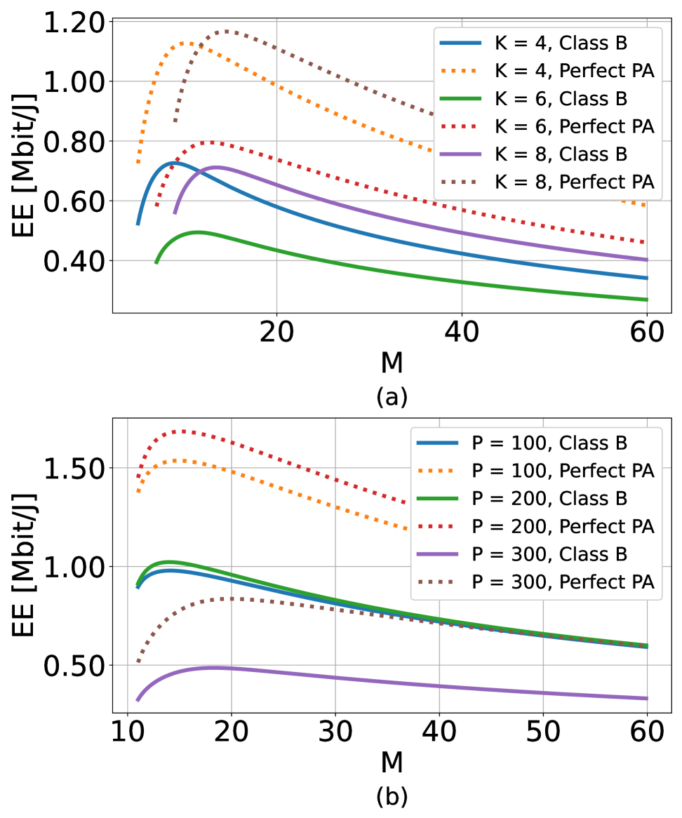
Figure 2: Plots of EE(M) for system parameters as used in Sec. V (see Table II) with fixed $P=200$ W and $K=10$ for figure a) and b), respectively. For each series, $\beta_{k}$ and $\omega_{k}$ is selected randomly from uniform distribution over $(60,150)$ dB, and a Dirichlet distribution with $\omega_{k}\geq 0$ and $\sum_{k}\omega_{k}=1$, respectively.

Observe that the function $EE(M)$ is non-convex due to the non-convexity of (10), as well as due to the fractional form of the objective function. Although it has been shown analytically in Appendix C that $f_{M}(M)\to+\infty$ as $M\to K^{+}$, whereas $f_{M}(M)\to 0^{-}$ as $M\to+\infty$, the behavior between these extreme points cannot be determined in closed-form. Despite this, extensive numerical evidence under diverse representative system parameters consistently shows that $EE(M)$ monotonically increases up to $M_{c}$ and decreases thereafter, strongly suggesting a single maximum and supporting the use of Proposition 1 for selecting $M^{*}$.

This is exemplified in Fig. 2, where EE(M) was plotted over $M$ while varying other parameters.

IV-C Alternating Optimization

The solutions of sub-problems presented in Sec. IV-A and Sec. IV-B can be used to solve the optimization problem (14) and (15), and thereby (13), by alternating optimization as shown in Algorithm 2. Firstly, for a fixed $M$ and $\boldsymbol{\omega}=[\omega_{1},\dots,\omega_{k}]$, we find the optimum solution for (16) via Algorithm 1 instantiated with $x\leftarrow P$. Then for the fixed M and with this optimum $P$, we find the optimum solution for (17) via well-known bisection method [27]. Finally, for the optimum $P$ and $\boldsymbol{\omega}$, we find the optimum $M$, i.e. solution to (15) via Algorithm 1 instantiated with $x\leftarrow M$. The process is repeated over multiple iterations of $P$ and $\boldsymbol{\omega}$, and $M$—with superscript $(i)$ denoting the solution at the $i$-th iteration—until convergence is achieved, i.e, until the difference between EE in the current and previous iteration is smaller than a non-negative value $\delta_{EE}$, which is the non-negative convergence tolerance. Finally, after finding solutions over the continuous domain, we evaluate EE at $\left\lfloor M\right\rfloor$ and $\left\lceil M\right\rceil$ and choose the one that results in the highest EE.

Algorithm 2 Alternating Optimization Framework for EE Maximization

1:Initialize: $i\leftarrow 0$, $\boldsymbol{\omega^{(i)}}=[\omega_{1}^{(i)},\dots,\omega_{K}^{(i)}]\leftarrow\frac{1}{K}$, $P\leftarrow P^{(i)}$, $M\leftarrow M^{(i)}$, threshold $\delta_{EE}$

2:repeat

3:  $i\leftarrow i+1$

4:  solve (16) given $M^{(i-1)}$ and $\boldsymbol{\omega^{(i-1)}}$ to get $P^{(i)}$ by Algorithm 1 for $f_{P}(P)$

5:  solve (17) given $M^{(i-1)}$ and $P^{(i)}$ to get $\boldsymbol{\omega^{(i)}}$ by bisection method [27]

6:  solve (15) given $P^{(i)}$ and $\boldsymbol{\omega^{(i)}}$ to get $M^{(i)}$ by Algorithm 1 for $f_{M}(M)$

7:  Compute: $\mathrm{EE}(P^{(i)},\boldsymbol{\omega^{(i)}},M^{(i)})$

8:until ${|\mathrm{EE}^{(i)}-\mathrm{EE}^{(i-1)}|<\delta_{EE}}$

9:if $\mathrm{EE}(P^{(i)},\boldsymbol{\omega^{(i)}},\left\lfloor M^{(i)}\right\rfloor)>\mathrm{EE}(P^{(i)},\boldsymbol{\omega^{(i)}},\left\lceil M^{(i)}\right\rceil)$ then

10:  $M^{*}\leftarrow\left\lfloor M^{(i)}\right\rfloor$

11:else

12:  $M^{*}\leftarrow\left\lceil M^{(i)}\right\rceil$

13:end if

V Simulation results

In this section, we evaluate the performance of the proposed DEEP-DEAL framework, considering both Class B PA and Perfect PA, under various scenarios and compare the results with certain benchmark algorithms, listed in Table I. We compare our results with a reference scenario, where the IBO $\Psi=6$ dB is fixed, ensuring that the SDR is high enough to guarantee the mean Error Vector Magnitude (EVM) of $4.5\%$ required in $5$G New Radio for $256$-QAM constellation [29]. Additionally, Table II shows the simulation parameters. It should be noted that in this section path loss in dB is denoted as $(\beta)_{\mathrm{dB}}$, which is related to the linear channel gain $\beta$ used in the previous sections as $\left(\beta\right)_{\mathrm{dB}}=-10\log_{10}(\beta)$.

DEEP-DEAL Distortion Aware Energy Efficient Power Allocation with Distortion Aware Energy Efficient Antenna Allocation DEEP Distortion Aware Energy Efficient Power Allocation with fixed Antenna Count REF-E Reference Power (IBO equals 6 dB) with Equal per UE Power Distribution and with fixed Antenna Count

TABLE I: Tested algorithms abbreviation summary.

$N_{\mathrm{U}}$ $\Delta f$ $\eta$ $(\sigma^{2})_{dBm}$ $1200$ $15$ kHz $\frac{2}{3}$ $-174\frac{dBm}{Hz}+10\cdot\log_{10}(N_{\mathrm{U}}\cdot\Delta f)$ $P_{\mathrm{const}}$ [5] $P_{\mathrm{SPRF}}$ [5] $P_{\textrm{max}}$ $(\beta_{k})_{\mathrm{dB}}$ [30] $348$ W $23$ W $160$ W $22.7+36.7\cdot\log_{10}(d_{k})+26\cdot\log_{10}(f_{c})$

TABLE II: Simulation parameters, where $d_{k}$ is the distance between UE $k$ and the base station in meters and $f_{c}=3$ GHz [30], and $\delta_{P}=\delta_{M}=\delta_{EE}=10^{-6}$.

V-A Two-UE Homogeneous Path Loss

With $K=2$ UEs, and $M=32$ antennas used for DEEP and REF-E algorithms, Fig. 3 shows how the EE changes over varying path loss, where both UEs have the same path loss, which, e.g., is possible when the UEs are at the same distance from the BS but on various azimuth angles. According to the path loss model in Table II, this range is equivalent to a wide distance range from 5 m to 2.3 km.

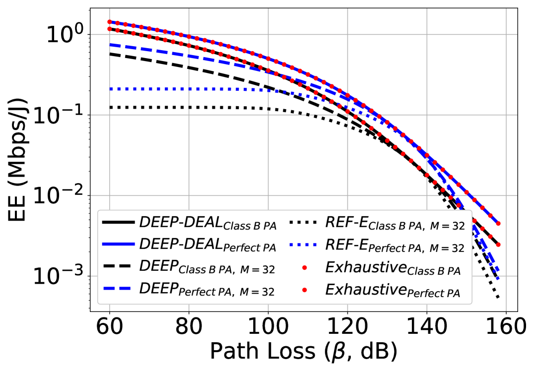
Figure 3: EE over varying path loss.

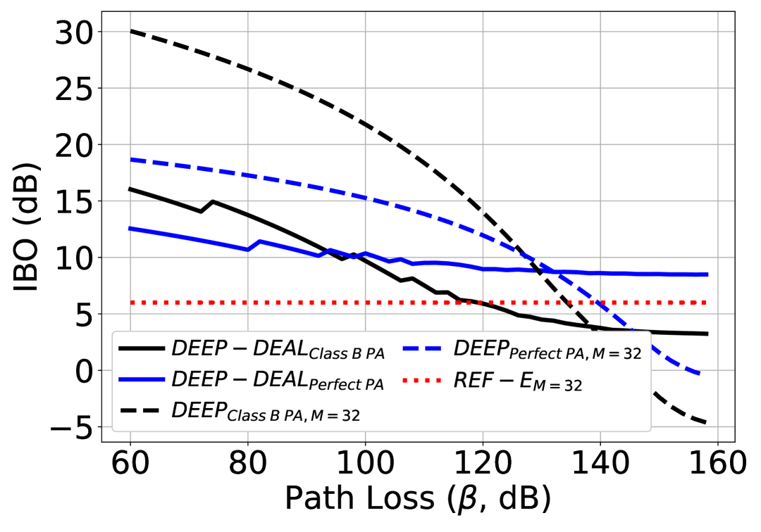
Figure 4: IBO over varying path loss.

Although for each scenario considered in Table I, the EE decreases as the distance from the BS increases and the channel worsens, our proposed DEEP-DEAL framework consistently outperforms both reference solutions, i.e., DEEP and REF-E, across all PA classes and path loss values. A critical path loss point (around $135$ dB in this case) is observed, where the combination of $M=32$ antennas and IBO of approximately $\Psi=6$ dB becomes optimal. At this point, the reference solution coincides with the optimal one. However, our proposed DEEP-DEAL scheme maintains distinct gains for both higher and lower path loss values. While the DEEP algorithm improves the EE—in comparison to REF-E—through optimal power allocation, additional improvements are obtained, e.g., up to $50\%$ in EE for Class B PA at $\beta_{dB}=80$, by optimizing the active number of antennas.

Moreover, observe in Fig. 3 that not only does DEEP-DEAL achieve better performance than the reference solutions, but it also matches the performance of the exhaustive search. The exhaustive search is performed testing all possible allocations of $M\in\{K+1,K+2,...,500\}$ and $P\in\{10,11,...,15000\}$ W. Since we consider a homogeneous UE scenario, $\omega_{k}=1/K$ is a trivial optimal solution, and does not need exhaustive research to be applied. Taken together, these results confirm the ability of the proposed method to reliably identify the global optimum.

The underlying nature of these gains can be understood by examining the optimal IBO and antenna count $M$. While REF-E operates with a fixed IBO of $\Psi=6$ dB, as shown in Fig. 4, schemes optimizing IBO exhibit a decreasing trend with increasing path loss. This implies that for short links, EE is maximized with low transmit power, which also generates a small amount of nonlinear distortion. Whereas, for long links, higher transmission power is required, resulting in lower IBO values (especially for the DEEP algorithm), though at the expense of stronger distortion.

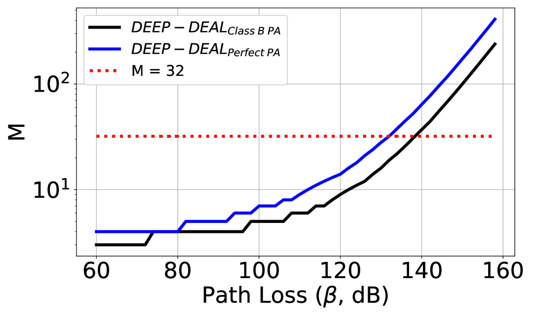
Figure 5: Optimal antenna count over varying path loss.

Most interesting is the behavior that emerges under the joint power and antenna count optimization, i.e., DEEP-DEAL. As reflected in Fig. 4, IBO no longer follows a monotonically decreasing trend. Instead, it exhibits a decrease-jump-decrease pattern with increasing path loss. This non-monotonicity reflects the system’s adaptive strategy to improve the EE by balancing both IBO and M. The sudden rise in IBO corresponds to the transitions where the optimal antenna count increases sharply. Eventually, for very high path loss, the optimal IBO with DEEP-DEAL stabilizes, though PA class dependent, reflecting that further EE improvements are obtained solely through antenna adaptation. Fig. 5 confirms this claim. For very short links, the optimal number of antennas reaches the system’s lower bound, i.e., $M=3$ (required for ZF with $2$ UEs), which grows rapidly with increasing path loss. However, the exact growth rate is PA class dependent, where Perfect PAs typically require more antennas. Examining both optimal IBO and number of antennas, it is visible that for very long links a higher power consumption, resulting from low IBO and a large number of active RF chains, is better than for shorter links. Thus, optimizing both IBO and antenna count is crucial for EE maximization.

V-B Two-UE Heterogeneous Path Loss

As depicted in Figs. 6, 8, 7, and 9, for the $2$ UE heterogeneous case, where each UE can experience a different path loss $\beta$, values are varied on a $2$-D grid from $60$ to $150$ dB. While the diagonal corresponds to the homogeneous path loss scenario discussed in Sec. V-A, the off-diagonal cases represent the heterogeneous scenario. It can be observed from Fig. 6 that our proposed DEEP-DEAL framework consistently outperforms REF-E, showing improvements in nearly all scenarios except when both UEs have path loss of around $140$ dB. In this case, no EE improvement is observed as the ratio equals $1$. This is the same situation as depicted in Fig. 3 when DEEP-DEAL result touches REF-E results. Though for higher path loss in Fig. 6, again EE gain is visible. In contrast, the largest gains are achieved when a single UE or both UEs are close to the BS, achieving $10$ times EE improvements in comparison to REF-E allocation.

The underlying mechanism of these gains can be understood by analyzing optimal power allocation, IBO, and antenna count. As reflected in Fig. 8, a funnel region of equal power allocation ($\omega_{1}=\omega_{2}=0.5$) emerges when both UEs experience comparable propagation conditions with a relatively large margin, i.e., extending for example to $(\beta_{1},\beta_{2})=(100,70)$ dB. Not only is the equal power allocation optimal in these quasi-homogeneous cases, but IBO and $M$ also follow a structured pattern, appearing as stripes perpendicular to the diagonal, as reflected in Fig. 7 and 9, respectively. In this region, optimal IBO and number of antennas $M$ allocation is primarily dependent on the sum of $(\beta_{1})_{dB}$ and $(\beta_{2})_{dB}$. Nevertheless, the main outcomes are similar to the ones described in Sec. V-A, i.e., optimal IBO decreases with increasing path loss, whereas optimal antenna count increases with increasing path loss. Note that the sharp transitions observed in IBO are artifacts of the integer-valued $M$ constraint imposed by the final step of the alternating optimization in Algorithm 2. Most interestingly, outside the equal power funnel, the system predominantly allocates the entire power to the UE closer to the BS. Thus, the stronger UE dictates the optimum IBO and antenna allocation. In general, the further away the UE, the lower is the optimal IBO (although some local non-monotonicity is visible as a result of combined M-IBO optimization), and the required number of antennas increases.

Figure 6: Class B PA - Ratio of DEEP-DEAL and REF-E EE for $2$ UEs over varying path loss with $M=32$ in REF-E $6$ dB scenario.

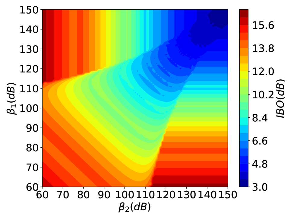
Figure 7: Class B PA - Optimum IBO by DEEP-DEAL for a $2$ UE scenario.

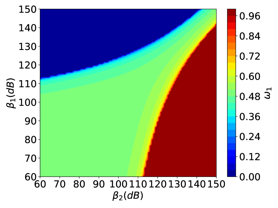
Figure 8: Class B PA - Fraction of power allocated by DEEP-DEAL to UE $1$ ($\omega_{1}$) for a $2$ UE scenario.

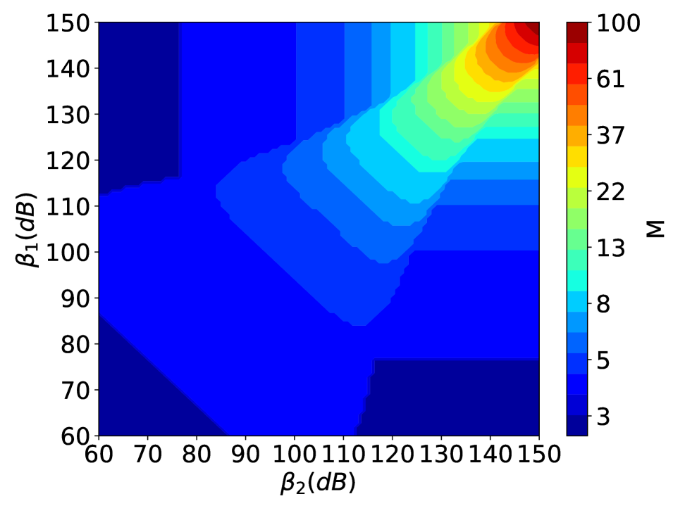
Figure 9: Class B PA - Optimum integer M by DEEP-DEAL for a $2$ UE scenario.

V-C Multi-UE Heterogeneous Path Loss

(a) EE CDF.

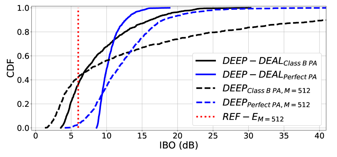
(b) IBO CDF.

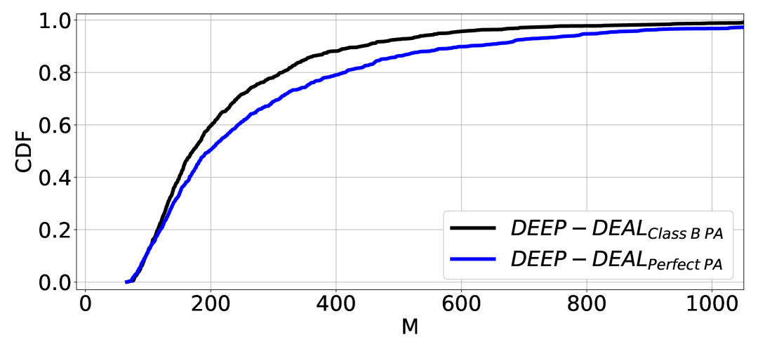
(c) Number of antennas $M$ CDF.

Figure 10: CDF performance metrics in a heterogeneous scenario with 60 UEs uniformly distributed in a 5 km radius cell.

Finally, in this scenario, the EE is evaluated within a single circular cell of 5 km radius where $K=60$ UEs are uniformly distributed. We generate $1000$ random UE location sets following the path loss model from Table II.

Fig. 10(a) and 10(b) show the cumulative distribution function (CDF) of EE and IBO, respectively, for the proposed and reference schemes under both PA architectures. It is observable that DEEP-DEAL outperforms all baselines for any percentile, where the largest gains are achieved in the high-EE region. EE gains at the median, relative to the REF-E scheme, reach approximately $40\%$ and $20\%$ for Perfect PA and Class BB PA, respectively, obtained by jointly fine-tuning the optimization variables. The corresponding IBO distribution highlights strong variability with PA class and UE positions. When antenna optimization is disabled, as in the case of DEEP, the optimal IBO is much higher—reaching $140$ dB for Class B PA—confirming the advantage of joint IBO-antenna optimization. Fig. 10(c) illustrates the distribution of the optimal number of antennas, which again depends on the PA class and UE positions. As observed, significantly more antennas are required with a realistic Class B PA. Although a minimal number of antennas is mandated to serve $60$ UE via ZF precoding, i.e., $M=61$, the optimal number is generally much larger, with the median around $150$-$160$ array elements.

VI Conclusion and Future Work

In this work, we first modeled the impact of soft-limiter PA characteristics on the EE of a MU-M-MIMO OFDM DL system employing ZF precoding under an i.i.d. Rayleigh channel. We defined the resource allocation problem and proposed the DEEP-DEAL framework, which jointly optimizes distortion-aware power control (DEEP) and antenna allocation (DEAL) in an alternating optimization manner. Unlike conventional formulations, the optimization problem does not require explicit transmit power constraints, as the nonlinear PA inherently limits the feasible operating region through distortion. Our simulation results show that DEEP-DEAL consistently outperforms distortion-neglecting and power-only optimizing baselines across homogeneous and heterogeneous UE scenarios and across PA classes. Notably, the optimum frequently operates at low (but non-negative) IBO, while jointly adapting the number of active antennas. This indicates that operating the PA near (but not beyond) saturation is EE-optimal when paired with antenna scaling. Overall, the findings underscore that balancing distortion-aware power control with antenna scaling is essential for maximizing EE in M-MIMO systems.

Several promising research directions emerge from this study. First, while DEEP-DEAL was evaluated for ZF precoding, extending the framework to other schemes such as MRT or hybrid precoding would provide further insights into its applicability under different interference and complexity trade-offs. Second, incorporating multi-cell scenarios with inter-cell interference and coordinated antenna activation could more closely reflect practical deployment conditions. Third, the present work assumes perfect CSI that can be extended to consider the channel estimation errors. Additionally, the optimization framework can be enriched by integrating traffic-aware or QoS-driven objectives, allowing energy-efficient adaptation to varying service demands. Finally, the hardware model can be extended, e.g., considering the envelope tracking PA, or distortions coming from different front-end elements like the DAC.

Appendix A Important Limits and Expansions

In the following Appendices, we employ the following limits [31]

$$\text{L1}:\lim_{x\to\infty}x^{a}e^{-x}=0\quad\forall a\in\mathbb{R},\ \quad\text{L2}:\lim_{x\to\infty}\mathrm{erf}(x)=1,$$

$$\text{L3}:\lim_{x\to\infty}x^{a}\mathrm{erfc}(x)=0\quad\forall a\in\mathbb{R}$$

and the following asymptotic expansions using Taylor series as $x\to 0$:

$$\text{A1}\!:\log_{2}(1+x)\sim\frac{x}{\ln(2)},\ \ \quad\quad\text{A2}\!:e^{-x}\sim 1-x+\frac{x^{2}}{2},$$

$$\text{A3}\!:\mathrm{erfc}(x)\!\sim\!1\!-\!\frac{2x}{\sqrt{\pi}}\!+\!\frac{2x^{3}}{3\sqrt{\pi}},\quad\text{A4}\!:\mathrm{erf}(x)\!\sim\!\frac{2x}{\sqrt{\pi}}\!-\!\frac{2x^{3}}{3\sqrt{\pi}}.$$

Note that we will use asymptotic expansion/equivalence [32] denoted by $\sim$.

Appendix B Proof of Lemma B

The partial derivative of $\frac{\partial{EE}}{\partial P}$ can be computed as

$$\frac{\partial\mathrm{{EE}}}{\partial P}=\frac{\sum_{k}\frac{\partial{R_{k}}}{\partial P}\cdot P_{\mathrm{tot}}-\sum_{k}R_{k}\cdot\frac{\partial P_{\mathrm{tot}}}{\partial P}}{P_{\mathrm{tot}}^{2}}.$$ (25)

Since $P_{\mathrm{tot}}$ is always positive, we focus only on the numerator of (25) that has to equal 0 to find the stationary point. This function has the same root as the function

$$f_{P}(P)=\frac{1}{\sum_{k}R_{k}}\sum_{k}\frac{\partial{R_{k}}}{\partial P}-\frac{1}{P_{\mathrm{tot}}}\frac{\partial P_{\mathrm{tot}}}{\partial P}$$ (26)

obtained by reordering components of the numerator of (25). Let $B=N_{\mathrm{U}}\Delta f$, then with $\gamma_{k}=\frac{(M-K)\lambda\omega_{k}P\beta_{k}}{\sigma_{k}^{2}+\beta_{k}D}$, $\frac{\partial{R_{k}}}{\partial P}$ can be computed as

$$\frac{\partial{R_{k}}}{\partial P}= \frac{B(M-K)}{\ln(2)\left(1+\gamma_{k}\right)}\frac{\omega_{k}\beta_{k}}{\left(\sigma_{k}^{2}+\beta_{k}D\right)^{2}}$$

$$\cdot\left(\left(\frac{\partial\lambda}{\partial P}P+\lambda\right)\left(\sigma_{k}^{2}+\beta_{k}D\right)-\lambda P\beta_{k}\frac{\partial D}{\partial P}\right),$$ (27)

where

$$\frac{\partial\lambda}{\partial P}= -\frac{\Psi\sqrt{\lambda}}{P}\left(e^{-\Psi}+\frac{1}{2}\sqrt{\frac{\pi}{\Psi}}\textrm{erfc}\left(\sqrt{\Psi}\right)\right),$$ (28)

and

$$\frac{\partial D}{\partial P}= \eta\left(1-e^{-\Psi}-\lambda-P\frac{\partial\lambda}{\partial P}-\Psi e^{-\Psi}\right),$$ (29)

recalling that IBO is defined as $\Psi=MP_{\mathrm{max}}/P$. Furthermore, observe that $\frac{\partial P_{\mathrm{tot}}}{\partial P}$ can be computed as

$$\frac{\partial P_{\mathrm{tot}}}{\partial P}=\frac{\partial P_{\mathrm{PA}}}{\partial P},$$ (30)

with

$$\frac{\partial P_{\mathrm{PA}}}{\partial P}=\begin{cases}\dfrac{\sqrt{\Psi}}{\sqrt{\pi}}\,\mathrm{erf}(\sqrt{\Psi})-\dfrac{2}{\pi}\Psi e^{-\Psi},&\textbf{Class B PA}\\ 1-e^{-\Psi}-\Psi e^{-\Psi},&\textbf{Perfect PA}\end{cases}$$ (31)

because the other components are independent of $P$.

In the following we aim to solve $f_{P}(P)=0$. Therefore, we show that (26) has at least a single root in the domain $P\geq 0$. To find the root, we analyze the asymptotic behavior of $f_{P}(P)$ as $P\to 0$ and $P\to\infty$ by employing the limits and asymptotic expansions defined in Appendix A.

Case 1 ($P\to 0$): Observe that as $P\to 0$, $\Psi\to\infty$, and therefore using L1 and L3 $\lim_{\Psi\to\infty}\lambda=1$ and $D=0$. With $\lambda=1$, $D=0$ and $P=\frac{MP_{\mathrm{max}}}{\Psi}$, $\gamma_{k}$ can be asymptotically expanded as

$$\gamma_{k}\sim\frac{M(M-K)\omega_{k}P_{\mathrm{max}}\beta_{k}}{\sigma^{2}_{k}\cdot\Psi}.$$ (32)

As $\Psi\to+\infty$, $\gamma_{k}\to 0$, and thus due to A1, $R_{k}$ simplifies to

$$R_{k}\sim\frac{BM(M-K)P_{\mathrm{max}}\omega_{k}\beta_{k}}{\ln(2)\sigma^{2}_{k}\Psi}$$ (33)

and therefore,

$$\sum_{k}R_{k}\sim\frac{BM(M-K)P_{\mathrm{max}}}{\ln(2)\Psi}\sum_{k}\frac{\omega_{k}\beta_{k}}{\sigma^{2}_{k}}.$$ (34)

Next observe that by substituting to L1 and L3 in (28) , $\frac{\partial\lambda}{\partial P}\to 0^{-}$ because the exponential term decays faster than any power of $\frac{1}{P}$ and $\frac{\partial D}{\partial P}\to 0$. Furthermore, as $\Psi\to\infty$, it is visible in (32) that $\gamma_{k}\to 0$, and therefore $(1+\gamma_{k})\to 1$. Thus

$$\frac{\partial{R_{k}}}{\partial P}\sim \frac{B(M-K)}{\ln(2)}\frac{\omega_{k}\beta_{k}}{\sigma_{k}^{2}}$$ (35)

and

$$\sum_{k}\frac{\partial{R_{k}}}{\partial P}\sim \frac{B(M-K)}{\ln(2)}\sum_{k}\frac{\omega_{k}\beta_{k}}{\sigma_{k}^{2}}.$$ (36)

Next, substituting the asymptotic expansion of the error function [31] as $x\to\infty$:

$$\mathrm{erf(x)}\sim 1-\frac{e^{-x^{2}}}{x\sqrt{\pi}}\left(1-\frac{1}{2x^{2}}\right)$$ (37)

in $\frac{\partial P_{\mathrm{PA}}}{\partial P}$ for Class B PA and using L1 for Perfect PA, (31) can be expanded as

$$\frac{\partial P_{\mathrm{PA}}}{\partial P}\sim\begin{cases}\frac{\sqrt{\Psi}}{\sqrt{\pi}},&\textbf{Class B PA}\\ 1&\textbf{Perfect PA}.\end{cases}$$ (38)

Moreover, note that in $P_{\mathrm{tot}}$, $P_{\mathrm{PA}}$ depends on $P$, while the other terms are independent. As $P\to 0$ and $\Psi\to\infty$, $P_{\mathrm{tot}}$ can be expanded as

$$\begin{cases}P_{\mathrm{tot}}\sim P_{const}+MP_{SPRF},&\textbf{Class B PA}\\ P_{\mathrm{tot}}\sim P+P_{\mathrm{const}}+MP_{\mathrm{SPRF}},&\textbf{Perfect PA}\end{cases}$$ (39)

because using (37) it can be easily shown that $P_{\mathrm{PA}}\to 0$ as $\Psi\to\infty$ for Class B PA, whereas, for Perfect PA (31) can be written as

$$P_{\mathrm{PA}}=\frac{MP_{\max}}{\Psi}(1-e^{-\Psi})=P\,(1-e^{-\Psi})$$ (40)

using the definition $\Psi=MP_{\max}/P$. As $\Psi\to\infty$, $(1-e^{-\Psi})\to 1$, and therefore $P_{\mathrm{PA}}\to P$. Finally, using (34), (36), (38), and (39), $f_{P}(P)$ after substituting $\Psi=MP_{\mathrm{max}}/P$ simplifies to

$$f_{P}(P) \sim\begin{cases}\frac{1}{\sqrt{P}}\left(\frac{1}{\sqrt{P}}-\frac{\sqrt{MP_{\mathrm{max}}}}{\sqrt{\pi}P_{\mathrm{tot}}}\right),&\textbf{Class B PA}\\ \frac{1}{P}-\frac{1}{P+P_{\mathrm{const}}+MP_{\mathrm{SPRF}}},&\textbf{Perfect PA}\end{cases}$$ (41)

showing that $f_{P}(P)\to+\infty$ as $P\to 0$.

Case 2 ($P\to\infty$): Observe that as $P\to\infty$, $\Psi\to 0$. As $\Psi\to 0$, using the first two monomials of A2 and A3 yields

$$\lambda \sim\left(\Psi+\frac{\sqrt{\pi\Psi}}{2}\left(1-\frac{2\sqrt{\Psi}}{\sqrt{\pi}}\right)\right)^{2}\sim\frac{\pi}{4}\Psi$$ (42)

Similarly $D$ can be asymptotically expanded using (42) and first two monomials of A2 as

$$D\!\sim\!\eta\left(\!1\!-\!(1\!-\!\Psi)\!-\!\frac{\pi\Psi}{4}\right)\frac{MP_{\mathrm{max}}}{\Psi}\!\sim\!\eta(1\!-\!\frac{\pi}{4})MP_{\mathrm{max}}.$$ (43)

While this is equal to $\lim_{P\to\infty}D$, it shows an interesting property: even when an OFDM signal of infinite mean power is applied to the PA input, the total (entire-band) distortion power from one front-end is limited to $(1-\frac{\pi}{4})P_{\mathrm{max}}$, i.e., about 20% of the saturation power.

Let us define the limit of nonlinear distortion and noise power at $k$-th UE for $P\to\infty$ as $C_{k}=\sigma^{2}_{k}+\eta\beta_{k}(1-\frac{\pi}{4})MP_{\mathrm{max}}$ using (43). Then $\gamma_{k}$ from (9) can be asymptotically expanded using first $P=\frac{MP_{\mathrm{max}}}{\Psi}$ and next (42) as

$$\!\!\!\gamma_{k} \!\sim\!\frac{M(M\!-\!K)\lambda\beta_{k}\omega_{k}P_{\mathrm{max}}}{C_{k}\cdot\Psi}\!\sim\!\frac{\pi M(M\!-\!K)\omega_{k}\beta_{k}P_{\mathrm{max}}}{4C_{k}},$$ (44)

which is a constant, non-negative value over $P$. Therefore, $\sum_{k}R_{k}=B\sum_{k}\log_{2}(1+\gamma_{k})$ is a positive constant. Next, as $\Psi\to 0$, it can be shown that substituting A2 and A3 in (28) and (29) yields

$$\frac{\partial\lambda}{\partial P}\sim-\frac{\pi\Psi}{4P}\;\text{and}\;\frac{\partial D}{\partial P}\sim\frac{\eta\Psi^{2}}{2},$$ (45)

and therefore, after substituting (42), (43), (44), and (45) in (B) and some simplifications

$$\frac{\partial{R_{k}}}{\partial P}\sim-\frac{BM(M-K)}{8\ln(2)\left(1+\gamma_{k}\right)}\frac{\eta\omega_{k}\beta_{k}^{2}\pi P_{\mathrm{max}}\Psi^{2}}{\left(\sigma_{k}^{2}+\beta_{k}D\right)^{2}}$$ (46)

and

$$\sum_{k}\frac{\partial{R_{k}}}{\partial P}\sim-\sum_{k}\frac{BM(M-K)}{8\ln(2)\left(1+\gamma_{k}\right)}\frac{\eta\omega_{k}\beta_{k}^{2}\pi P_{\mathrm{max}}\Psi^{2}}{\left(\sigma_{k}^{2}+\beta_{k}D\right)^{2}}.$$ (47)

Next, using A2 and A4 in $\frac{\partial P_{\mathrm{PA}}}{\partial P}$, (31) can be expanded as

$$\begin{cases}\frac{\partial P_{\mathrm{PA}}}{\partial P}\sim\frac{4\Psi^{2}}{3\pi}-\frac{\Psi^{3}}{\pi}\sim 0,&\textbf{Class B PA}\\ \frac{\partial P_{\mathrm{PA}}}{\partial P}\sim\frac{\Psi^{2}}{2}-\frac{\Psi^{3}}{2}\sim 0&\textbf{Perfect PA}\end{cases}$$ (48)

and thus, $\frac{1}{P_{\mathrm{tot}}}\frac{\partial P_{\mathrm{tot}}}{\partial P}$ results in $0$. Finally, using the derivations above, $f_{P}(P)$ simplifies to

$$f_{P}(P) \sim-\frac{1}{\sum_{k}\log_{2}(1+\gamma_{k})}\cdot$$

$$\sum_{k}\frac{BM(M-K)}{8\ln(2)\left(1+\gamma_{k}\right)}\frac{\eta\omega_{k}\beta_{k}^{2}\pi P_{\mathrm{max}}\Psi^{2}}{\left(\sigma_{k}^{2}+\beta_{k}D\right)^{2}}$$ (49)

and $f_{P}(P)\to 0^{-}$ as $P\to+\infty$ and $\Psi\to 0$. Thus, by Intermediate Value Theorem there must exist at least one root in $(0,+\infty)$ for both Class B and Perfect PA.

Appendix C Proof of Lemma C

Assuming $EE$ function can be relaxed over $M$ the partial derivative of $\frac{\partial{EE}}{\partial M}$ can be computed as

$$\frac{\partial\mathrm{{EE}}}{\partial M}=\frac{\sum_{k}\frac{\partial{R_{k}}}{\partial M}\cdot P_{\mathrm{tot}}-\sum_{k}R_{k}\cdot\frac{\partial P_{\mathrm{tot}}}{\partial M}}{P_{\mathrm{tot}}^{2}}.$$ (50)

Since $P_{\mathrm{tot}}$ is always positive, we focus only on the numerator of (50) that has to equal 0 to find the stationary point. This function has the same root as the function

$$f_{M}(M)=\frac{1}{\sum_{k}R_{k}}\sum_{k}\frac{\partial{R_{k}}}{\partial M}-\frac{1}{P_{\mathrm{tot}}}\frac{\partial P_{\mathrm{tot}}}{\partial M}.$$ (51)

Let $B=N_{\mathrm{U}}\Delta f$, then with $\gamma_{k}=\frac{(M-K)\lambda\omega_{k}P\beta_{k}}{\sigma_{k}^{2}+\beta_{k}D}$, $\frac{\partial{R_{k}}}{\partial M}$ equals

$$\frac{\partial R_{k}}{\partial M}=\frac{B\beta_{k}P\omega_{k}}{\ln(2)\left(1+\gamma_{k}\right)}\frac{1}{(\sigma^{2}_{k}+\beta_{k}D)^{2}}\cdot$$ (52)

$$\left[\left(\lambda+(M-K)\frac{\partial\lambda}{\partial M}\right)(\sigma^{2}_{k}+\beta_{k}D)-(M-K)\lambda\beta_{k}\frac{\partial D}{\partial M}\right],$$

where

$$\frac{\partial\lambda}{\partial M}=\sqrt{\lambda}\frac{P_{\mathrm{max}}}{P}\left(e^{-\Psi}+\frac{1}{2}\sqrt{\frac{\pi}{\Psi}}\mathrm{erfc}(\sqrt{\Psi})\right)$$ (53)

and

$$\frac{\partial D}{\partial M}=\eta\left({P_{\mathrm{max}}e^{-\Psi}}-P\frac{\partial\lambda}{\partial M}\right).$$ (54)

Furthermore, observe that $\frac{\partial P_{\mathrm{tot}}}{\partial M}$ can be computed as

$$\frac{\partial P_{\mathrm{tot}}}{\partial M}=\frac{\partial P_{\mathrm{PA}}}{\partial M}+P_{SPRF}$$ (55)

with

$$\frac{\partial P_{\mathrm{PA}}}{\partial M}=\begin{cases}\frac{2P_{\mathrm{max}}}{\sqrt{\pi}}\left(\frac{\mathrm{erf}(\sqrt{\Psi})}{2\sqrt{\Psi}}+\frac{e^{-\Psi}}{\sqrt{\pi}}\right)&\textbf{Class B PA}\\ P_{\mathrm{max}}e^{-\Psi}&\textbf{Perfect PA}.\end{cases}$$ (56)

To prove we can always find a root, we analyze the asymptotic behavior of $f_{M}(M)$ as $M\to K^{+}$ and $M\to\infty$ by employing the approximations defined in Appendix A.

Case 1 ($M\to K^{+}$): Observe that as $M\to K^{+}$, $\Psi\to\Psi_{0}$, where $\Psi_{0}=\frac{KP_{\mathrm{max}}}{P}$, $\lambda\to\lambda_{0}$, which is computed as

$$\lambda_{0}\!=\!\left(\!1\!-\!e^{-\Psi_{0}}\!\!+\!\!\frac{1}{2}\sqrt{\pi\Psi_{0}}\mathrm{\textrm{erfc}}\left(\sqrt{\Psi_{0}}\right)\!\right)^{2}\!,$$ (57)

and $D\to D_{0}$, computed as

$$D_{0}=\eta(1-e^{-\Psi_{0}}-\lambda_{0})P.$$ (58)

Furthermore, observe that $\gamma_{k}=\frac{(M-K)\lambda\omega_{k}P\beta_{k}}{\sigma_{k}^{2}+\beta_{k}D}\to 0$ as the denominator is positive, but $(M-K)\to 0$. Thus, using A1

$$R_{k}\sim\frac{B(M-K)P}{\ln(2)}\frac{\lambda_{0}\omega_{k}\beta_{k}}{(\sigma^{2}_{k}+\beta_{k}D_{0})},$$ (59)

resulting in

$$\sum_{k}R_{k}\sim\frac{B(M-K)P}{\ln(2)}\sum_{k}\frac{\lambda_{0}\omega_{k}\beta_{k}}{(\sigma^{2}_{k}+\beta_{k}D_{0})},$$ (60)

which vanishes as $M\to K^{+}$ since $\sum_{k}R_{k}$ is proportional to $(M-K)$. Next observe that as $M\to K^{+}$, $\frac{\partial R_{k}}{\partial M}$ can be approximated as

$$\frac{\partial R_{k}}{\partial M}\sim\frac{BP}{\ln(2)}\frac{\lambda_{0}\beta_{k}\omega_{k}}{(\sigma^{2}_{k}+\beta_{k}D_{0})}$$ (61)

because $\gamma_{k}\to 0$ and $\left.\frac{\partial\lambda}{\partial M}\right|_{\Psi=\Psi_{0}}$ and $\left.\frac{\partial D}{\partial M}\right|_{\Psi=\Psi_{0}}$ are finite constants, which when multiplied with $(M-K)\to 0^{+}$ terms in (52) vanish. Hence, summation over all UEs results in

$$\sum_{k}\frac{\partial R_{k}}{\partial M}\sim\frac{BP}{\ln(2)}\sum_{k}\frac{\lambda_{0}\beta_{k}\omega_{k}}{(\sigma^{2}_{k}+\beta_{k}D_{0})}.$$ (62)

Next we analyze $\frac{\partial P_{\mathrm{PA}}}{\partial M}$. As $M\to K^{+}$, $\Psi\to\Psi_{0}$, therefore $\frac{\partial P_{\mathrm{PA}}}{\partial M}$ is a constant, computed as

$$\frac{\partial P_{\mathrm{PA}}}{\partial M}\!\!=\!\!\begin{cases}\!\frac{2P_{\mathrm{max}}}{\sqrt{\pi}}\!\left(\!\frac{\mathrm{erf}(\sqrt{\Psi_{0}})}{2\sqrt{\Psi_{0}}}\!+\!\frac{e^{-\Psi_{0}}}{\sqrt{\pi}}\!\right)\!\!=:\!\Theta_{1},&\textbf{Class B PA}\\ \!P_{\mathrm{max}}e^{-\Psi_{0}}\!=:\!\Theta_{2}&\textbf{Perfect PA}\end{cases}$$ (63)

leading to $\frac{\partial P_{\mathrm{tot}}}{\partial M}$ being a constant

$$\frac{\partial P_{\mathrm{tot}}}{\partial M}\!\!=\!\!\begin{cases}\!\Theta_{1}\!+\!P_{\mathrm{SPRF}},&\textbf{Class B PA}\\ \!\Theta_{2}\!+\!P_{\mathrm{SPRF}},&\textbf{Perfect PA}\end{cases}$$ (64)

for both Class B PA and Perfect PA. Similarly, $P_{\mathrm{PA}}$ is a constant, which can be computed as

$$P_{\mathrm{PA}}=\begin{cases}\frac{2KP_{\mathrm{max}}}{\sqrt{\pi\Psi_{0}}}\mathrm{erf}(\sqrt{\Psi_{0}})=:K\Theta_{3},&\textbf{Class B PA}\\ \frac{KP_{\mathrm{max}}}{\Psi_{0}}(1-e^{-\Psi_{0}})=:K\Theta_{4}&\textbf{Perfect PA}\end{cases}$$ (65)

and thus

$$P_{\mathrm{tot}}=\begin{cases}K\left(\Theta_{3}+P_{\mathrm{SPRF}}\right)+P_{\mathrm{const}},&\textbf{Class B PA}\\ K\left(\Theta_{4}+P_{\mathrm{SPRF}}\right)+P_{\mathrm{const}}&\textbf{Perfect PA}.\end{cases}$$ (66)

The above equations justify that

$$\frac{1}{P_{\mathrm{tot}}}\frac{\partial P_{\mathrm{tot}}}{\partial M}=\mathrm{const}.$$ (67)

Therefore, substituting (60), (62), and (67) to (51), the function

$$f_{M}(M)\sim\frac{1}{M-K}-\mathrm{const},$$ (68)

which approaches $+\infty$ as $M\to K^{+}$.

Case 2 ($M\to\infty$): Observe that as $M\to\infty$, $\Psi\to\infty$ and therefore, using L1-L3, $\lambda\to 1$ and $D\to 0$.

With these assumptions, the SINR $\gamma_{k}\to\infty$ and thus, the achievable rate can be asymptotically expanded. First observe that $\log_{2}(1+\gamma_{k})=\log_{2}(\gamma_{k})+\log_{2}\!\left(1+\frac{1}{\gamma_{k}}\right)$. From A1 $\log_{2}\!\left(1+\tfrac{1}{\gamma_{k}}\right)\sim\tfrac{1}{\gamma_{k}\ln 2}\to 0$ as $\gamma_{k}\to\infty$, it follows that $\log_{2}(1+\gamma_{k})\sim\log_{2}(\gamma_{k})$. Therefore, the achievable rate can be asymptotically expanded as

$$R_{k}\sim B\log_{2}\left(\frac{(M-K)P\omega_{k}\beta_{k}}{\sigma^{2}_{k}}\right).$$ (69)

Additionally, as $M\to\infty$, $\lambda\to 1$, thus $\sqrt{\lambda}$ stays bounded. Moreover for $(M-K)\frac{\partial\lambda}{\partial M}$ in (52), using $M=\Psi P/P_{\mathrm{max}}$, L1, and L3 with $a=1$, observe that $(M\!-\!K)\,e^{-\Psi}\to 0$ and $(M\!-\!K)\,\sqrt{\tfrac{1}{\Psi}}\,\mathrm{erfc}(\sqrt{\Psi})=\left(\frac{\sqrt{\Psi}P}{P_{\mathrm{max}}}-\frac{K}{\sqrt{\Psi}}\right)\mathrm{erfc}(\sqrt{\Psi})\to 0-0=0$. Following similar reasoning $(M\!-\!K)\,\frac{\partial D}{\partial M}\to 0$, and hence all terms proportional to $(M\!-\!K)\,\frac{\partial\lambda}{\partial M}$ and $(M\!-\!K)\,\frac{\partial D}{\partial M}$ vanish as $M\to\infty$. When substituted to (52), we obtain

$$\frac{\partial R_{k}}{\partial M}\sim\frac{B\beta_{k}P\omega_{k}\sigma^{2}_{k}}{\ln(2)\left(\frac{(M-K)P\omega_{k}\beta_{k}}{\sigma^{2}_{k}}\right)}\frac{1}{\sigma^{4}_{k}}\sim\frac{B}{(M-K)\ln(2)},$$ (70)

resulting in

$$\frac{\sum_{k}\frac{\partial R_{k}}{\partial M}}{\sum_{k}R_{k}}\sim\frac{1}{\ln(2)(M-K)\sum_{k}\log_{2}\left(\frac{(M-K)P\omega_{k}\beta_{k}}{\sigma^{2}_{k}}\right)}.$$ (71)

As $M\to\infty$, $M\gg K$, and thus, $\frac{\sum_{k}\frac{\partial R_{k}}{\partial M}}{\sum_{k}R_{k}}$ can be expanded as

$$\frac{\sum_{k}\frac{\partial R_{k}}{\partial M}}{\sum_{k}R_{k}}\sim\frac{1}{\ln(2)M\sum_{k}\log_{2}\left(\frac{MP\omega_{k}\beta_{k}}{\sigma^{2}_{k}}\right)}.$$ (72)

Similarly, as $M$ and $\Psi$ $\to\infty$, using L1-L3 yields

$$\frac{\partial P_{\mathrm{PA}}}{\partial M}\sim\begin{cases}0,&\textbf{Class B PA}\\ 0&\textbf{Perfect PA}\end{cases}$$ (73)

and therefore $\frac{\partial P_{\mathrm{tot}}}{\partial M}$ is a constant

$$\frac{\partial P_{\mathrm{tot}}}{\partial M}\sim P_{SPRF}$$ (74)

for both Class B and Perfect PA. Next, $P_{\mathrm{PA}}$ can be expanded using the substitution $MP_{\mathrm{max}}=\Psi P$, and then L1 or L3 and $\mathrm{erf}(x)=1-\mathrm{erfc}(x)$ relation as

$$P_{\mathrm{PA}}\sim\begin{cases}\sqrt{\frac{4\Psi P^{2}}{{\pi}}},&\textbf{Class B PA}\\ P.&\textbf{Perfect PA}\end{cases}$$ (75)

Thus, using substitution $\Psi P=MP_{\mathrm{max}}$ we get

$$P_{\mathrm{tot}}\sim\begin{cases}\sqrt{\frac{4MP_{\mathrm{max}}P}{{\pi}}}+MP_{SPRF},&\textbf{Class B PA}\\ P+MP_{SPRF}&\textbf{Perfect PA}.\end{cases}$$ (76)

Finally, combining everything above, and factoring $1/M$, $f_{M}(M)$ becomes

$$f_{M}(M) \sim\frac{1}{M}\Bigg[\frac{1}{\ln(2)\sum_{k}\log_{2}\left(\frac{MP\omega_{k}\beta_{k}}{\sigma^{2}_{k}}\right)}-$$

$$\begin{cases}\frac{P_{SPRF}}{\sqrt{\frac{4P_{\mathrm{max}}P}{{\pi M}}}+P_{SPRF}},&\textbf{Class B PA}\\ \frac{P_{SPRF}}{\frac{P}{M}+P_{SPRF}}.&\textbf{Perfect PA}\end{cases}\Bigg]$$ (77)

Observe that the first component under brackets goes to $0$ as $M\to\infty$. At the same time, as $M\to\infty$, the second component, both for Class B PA and Perfect PA goes to $1$. This leads to $f_{M}(M)\sim-\frac{1}{M}$ and thus $f_{M}(M)$ approaches $0^{-}$ as $M\to\infty$. Since $f_{M}(M)\to+\infty$ as $M\to 0$ and $f_{M}(M)\to 0^{-}$ as $M\to\infty$, by the Intermediate Value Theorem, there must exist at least one root in $(0,+\infty)$.

References

- [1] E. Björnson, J. Hoydis, M. Kountouris, and M. Debbah, “Massive MIMO Systems with Non-ideal Hardware: Energy Efficiency, Estimation, and Capacity Limits,” IEEE Transactions on information theory, vol. 60, no. 11, pp. 7112–7139, 2014.
- [2] D. López-Pérez, A. De Domenico, N. Piovesan, G. Xinli, H. Bao, S. Qitao, and M. Debbah, “A Survey on 5G Radio Access Network Energy Efficiency: Massive MIMO, Lean Carrier Design, Sleep Modes, and Machine Learning,” IEEE Communications Surveys & Tutorials, vol. 24, no. 1, pp. 653–697, 2022.
- [3] Q. Wu, G. Y. Li, W. Chen, D. W. K. Ng, and R. Schober, “An Overview of Sustainable Green 5G Networks,” IEEE Wireless Communications, vol. 24, no. 4, pp. 72–80, 2017.
- [4] S. Zhang, Q. Wu, S. Xu, and G. Y. Li, “Fundamental Green Tradeoffs: Progresses, Challenges, and Impacts on 5G Networks,” IEEE Communications Surveys & Tutorials, vol. 19, no. 1, pp. 33–56, 2017.
- [5] S. Marwaha, E. A. Jorswieck, M. S. Jassim, T. Kürner, D. L. Pérez, X. Geng, and H. Bao, “Energy Efficient Operation of Adaptive Massive MIMO 5G HetNets,” IEEE Transactions on Wireless Communications, vol. 23, no. 7, pp. 6889–6904, 2024.
- [6] E. Björnson, L. Sanguinetti, J. Hoydis, and M. Debbah, “Designing Multi-User MIMO for Energy Efficiency: When is Massive MIMO the Answer?” in 2014 IEEE Wireless Communications and Networking Conference (WCNC), 2014, pp. 242–247.
- [7] M. M. A. Hossain, C. Cavdar, E. Björnson, and R. Jäntti, “Energy Saving Game for Massive MIMO: Coping With Daily Load Variation,” IEEE Transactions on Vehicular Technology, vol. 67, no. 3, pp. 2301–2313, 2018.
- [8] P. Kryszkiewicz, “Efficiency Maximization for Battery-Powered OFDM Transmitter via Amplifier Operating Point Adjustment,” Sensors, vol. 23, no. 1, p. 474, 2023.
- [9] E. Björnson, M. Matthaiou, and M. Debbah, “Massive MIMO Systems with Hardware-Constrained Base Stations,” in 2014 IEEE International Conference on Acoustics, Speech and Signal Processing (ICASSP), 2014, pp. 3142–3146.
- [10] G. Miao, N. Himayat, Y. Li, and D. Bormann, “Energy Efficient Design in Wireless OFDMA,” in 2008 IEEE International Conference on Communications, 2008, pp. 3307–3312.
- [11] E. Björnson, L. Sanguinetti, J. Hoydis, and M. Debbah, “Optimal Design of Energy-Efficient Multi-User MIMO Systems: Is Massive MIMO the Answer?” IEEE Transactions on Wireless Communications, vol. 14, no. 6, pp. 3059–3075, 2015.
- [12] Z. Liu, C.-H. Lee, W. Xu, and S. Li, “Energy-Efficient Design for Massive MIMO With Hardware Impairments,” IEEE Transactions on Wireless Communications, vol. 20, no. 2, pp. 843–857, 2021.
- [13] M. Parvini, B. Banerjee, M. Q. Khan, A. Nimr, and G. Fettweis, “Energy Efficiency vs Spectral Efficiency Tradeoff in MIMO Systems with Hardware Non-Linearities,” in 2025 Joint European Conference on Networks and Communications & 6G Summit (EuCNC/6G Summit), 2025, pp. 1–6.
- [14] 3GPP, “Study on network energy savings for NR (Release 18),” 3rd Generation Partnership Project (3GPP), Technical Report 38.864, March 2023, v18.1.0. [Online]. Available: https://www.3gpp.org/ftp/Specs/archive/38_series/38.864/38864-i10.zip
- [15] S. Marwaha, P. Kryszkiewicz, and E. Jorswieck, “Optimal Distortion-Aware Multi-User Power Allocation for Massive MIMO Networks,” 2025. [Online]. Available: https://arxiv.org/abs/2509.06491
- [16] C. Mollén, U. Gustavsson, T. Eriksson, and E. G. Larsson, “Spatial Characteristics of Distortion Radiated From Antenna Arrays With Transceiver Nonlinearities,” IEEE Transactions on Wireless Communications, vol. 17, no. 10, pp. 6663–6679, 2018.
- [17] M. Wachowiak and P. Kryszkiewicz, “Clipping Noise Cancellation Receiver for the Downlink of Massive MIMO OFDM System,” IEEE Transactions on Communications, vol. 71, no. 10, pp. 6061–6073, 2023.
- [18] E. Björnson, J. Hoydis, and L. Sanguinetti, “Massive MIMO Networks: Spectral, Energy, and Hardware Efficiency,” Foundations and Trends® in Signal Processing, vol. 11, no. 3-4, pp. 154–655, 2017. [Online]. Available: http://dx.doi.org/10.1561/2000000093
- [19] S. Wei, D. L. Goeckel, and P. A. Kelly, “Convergence of the Complex Envelope of Bandlimited OFDM Signals,” IEEE Transactions on Information Theory, vol. 56, no. 10, pp. 4893–4904, 2010.
- [20] R. Raich, H. Qian, and G. T. Zhou, “Optimization of SNDR for Amplitude-Limited Nonlinearities,” IEEE Transactions on Communications, vol. 53, no. 11, pp. 1964–1972, 2005.
- [21] J. Joung, C. K. Ho, K. Adachi, and S. Sun, “A Survey on Power-Amplifier-Centric Techniques for Spectrum- and Energy-Efficient Wireless Communications,” IEEE Communications Surveys & Tutorials, vol. 17, no. 1, pp. 315–333, 2015.
- [22] M. B. Salman, E. Björnson, G. M. Güvensen, and T. Çiloğlu, “Analytical Nonlinear Distortion Characterization for Frequency-Selective Massive MIMO Channels,” in ICC 2023 - IEEE International Conference on Communications, 2023, pp. 6535–6540.
- [23] T. Lee and H. Ochiai, “Characterization of Power Spectral Density for Nonlinearly Amplified OFDM Signals based on Cross-Correlation Coefficient,” EURASIP Journal on Wireless Communications and Networking, vol. 2014, pp. 1–15, 2014.
- [24] H. Ochiai, “An Analysis of Band-Limited Communication Systems from Amplifier Efficiency and Distortion Perspective,” IEEE Transactions on Communications, vol. 61, no. 4, pp. 1460–1472, 2013.
- [25] J. Guerreiro, R. Dinis, and P. Montezuma, “On the Optimum Multicarrier Performance with Memoryless Nonlinearities,” IEEE Transactions on Communications, vol. 63, no. 2, pp. 498–509, 2015.
- [26] A. Zappone and E. A. Jorswieck, “Energy Efficiency in Wireless Networks via Fractional Programming Theory,” Foundations and Trends in Communications and Information Theory, vol. 11, no. 3-4, pp. 185–396, 2014.
- [27] S. Boyd and L. Vandenberghe, Convex Optimization. Cambridge University Press, 2004.
- [28] C. Xing, Y. Jing, S. Wang, S. Ma, and H. V. Poor, “New Viewpoint and Algorithms for Water-Filling Solutions in Wireless Communications,” IEEE Transactions on Signal Processing, vol. 68, pp. 1618–1634, 2020.
- [29] 3GPP, “3rd Generation Partnership Project;Technical Specification Group Radio Access Network; NR; Base Station (BS) conformance testing Part 1: Conducted conformance testing (Release 18),” 3GPP, Tech. Rep. TS 38.141-1 V18.7.0, 2024.
- [30] International Telecommunication Union, “Guidelines for Evaluation of Radio Interface Technologies for IMT-Advanced,” International Telecommunication Union, Tech. Rep. M.2135-1, 2009. [Online]. Available: https://www.itu.int/dms_pub/itu-r/opb/rep/r-rep-m.2135-1-2009-pdf-e.pdf
- [31] M. Abramowitz and I. A. Stegun, Handbook of Mathematical Functions with Formulas, Graphs, and Mathematical Tables. New York: Dover Publications, 1964, originally issued by the National Bureau of Standards in 1964 as Applied Mathematics Series 55 (AMS 55).
- [32] D. Tse and P. Viswanath, Fundamentals of wireless communication. Cambridge university press, 2005.