Nonlinear Heisenberg Limit via Uncertainty Principle in Quantum Metrology

Abstract

The Heisenberg limit is acknowledged as the ultimate precision limit in quantum metrology, traditionally implying that root mean square errors of parameter estimation decrease linearly with the time $T$ of evolution and the number $N$ of quantum gates or probes. However, this conventional perspective fails to interpret recent studies of “super-Heisenberg” scaling, where precision improves faster than linearly with $T$ and $N$. In this work, we revisit the Heisenberg scaling by leveraging the position-momentum uncertainty relation in parameter space and characterizing precision in terms of the corresponding canonical momentum. This reformulation not only accounts for time and energy resources, but also incorporates underlying resources arising from noncommutativity and quantum superposition. By introducing a generating process with indefinite time direction, which involves noncommutative quantum operations and superposition of time directions, we obtain a quadratic increment in the canonical momentum, thereby achieving a nonlinear-scaling precision limit with respect to $T$ and $N$. Then we experimentally demonstrate in quantum optical systems that this nonlinear-scaling enhancement can be achieved with a fixed probe energy. Our results provide a deeper insight into the Heisenberg limit in quantum metrology, and shed new light on enhancing precision in practical quantum metrological and sensing tasks.

I Introduction

Quantum metrology holds importance in fundamental physics and diverse technical applications. Notably, quantum metrological principles have already been used in the Laser Interferometer Gravitational-Wave Observatory (LIGO)[1, 2, 3], navigation technologies[4, 5, 6], and biochemical applications[7, 8]. The central task in quantum metrology is to determine the ultimate precision limit in estimating unknown parameters. Traditionally, the Heisenberg limit has been regarded as the ultimate precision limit for quantum parameter estimation[9, 10, 11], characterized by a scaling of $1/\mathcal{H}$, where $\mathcal{H}$ denotes resource costs on time or energy, typically qualified in terms of the evolution time $T$ of the probe state[12] or the number $N$ of probes/quantum gates[13, 14, 15, 16, 17].

However, recent studies have demonstrated the possibility of surpassing the conventional Heisenberg limit—achieving so-called “super-Heisenberg” scaling, in which the precision improves faster than linearly with respect to $T$ or $N$—through several approaches. These include nonlinear interactions among probes[18, 19, 20], adaptive control within specific time-dependent Hamiltonians[21, 22], non-Markovian correlations between metrological processes[23, 24] or indefinite causal order (ICO) of phase-space displacements in estimating geometric phase[25, 26]. While it has been argued that scenarios involving nonlinear interactions still consist with the scaling $1/\mathcal{H}$ when all resources are properly accounted for[27, 28, 29, 30, 31, 32], this conventional perspective of Heisenberg scaling fails to interpret other instances of “super-Heisenberg” scaling. The underlying physical mechanisms and resource considerations that enable such nonlinear enhancements remain to be fully elucidated.

Building upon the uncertainty relation between position and momentum in parameter space[33, 34, 35, 36], we reformulate the Heisenberg scaling as $1/\Delta\bar{\mathcal{K}}$, where $\mathcal{K}$ denotes the canonical momentum conjugate to the parameter and $1/\Delta\bar{\mathcal{K}}$ represents its average uncertainty on the quantum state employed. This generalized formulation unifies a variety of “super-Heisenberg” regimes, as the canonical momentum $\mathcal{K}$ is not restricted to conventional physical resources in terms of time or energy. Instead, it can even encompass quantum resources arising from noncommutativity and superpositions of causal orders, thereby enabling nonlinear increases in $\Delta\bar{\mathcal{K}}$ with respect to $T$ or $N$.

Furthermore, we bridge the canonical momentum with the dynamical characteristic operator $\hat{V}_{S}=\partial_{g}\hat{H}_{S}$ of the parameterizing process, where $\hat{H}_{S}$ is the corresponding Hamiltonian. We derive that, in ancilla-free quantum metrological schemes, $\Delta\bar{\mathcal{K}}$ cannot increase faster than linearly with $T$ or $N$ if the average uncertainty of $\hat{V}_{S}$ (denoted as $\Delta\bar{V}_{S}$) is bounded. This motivates us to develop a general framework for achieving nonlinear-scaling enhancements in quantum metrology by utilizing ancillas. Specifically, we identify the quantum switch implemented by an external ancilla is a promising and experimentally accessible strategy. Of special interest is the indefinite time direction (ITD) enabled by the quantum switch, which allows the probe to evolve through a coherent superposition of forward and backward time directions[37]. This technique has demonstrated its ability to enhance various quantum information processing tasks, including quantum discrimination and quantum games[38, 39], and has shown potential in maximizing resource utilization in quantum metrology[40].

In this work, we devise a generating process prior to the unitary parameterizing process, with a Hamiltonian that is conjugate to the characteristic operator $\hat{V}_{S}$. The resulting noncommutativity leads to a nonlinear increment in the canonical momentum. We further incorporate the indefinite-time-direction strategy into the generating process, whereby the superposition of time directions converts the increment in the canonical momentum into an increase in its uncertainty. By matching the time length of the generating process and that of the parameterizing process, our scheme achieves a nonlinear scaling of $\delta g\propto T^{-2}$. Notably, we achieve this nonlinear-scaling enhancement within a time-independent Hamiltonian, which is traditionally believed unattainable. Furthermore, by sequentially applying the generating and parameterizing processes $N$ times, the precision limit can also exhibit a nonlinear scaling of $\delta g\propto N^{-2}$.

Experimentally, we implement our scheme in a quantum optical system for practically measuring the rotation angle of the photon beam’s profile. It noteworthy that the physical properties of photons in quantum optical systems offer a wide range of resources, such as polarization, spatial mode[41, 42, 43], and orbital angular momentum (OAM)[44], while do not involve real-world energy since photons have no rest mass. By using Q-plates[45] to implement the generating process with indefinite time direction for increasing the OAM of photons, we demonstrate that the precision limit is improved quadratically with the evolution time length $T$ and processes number $N$. Our experimental results confirm that the proposed scheme can achieve the desired precision enhancement efficiently. Consequently, our findings offer a profound and intuitive understanding of the Heisenberg limit, and establish a novel pathway for achieving nonlinear-scaling precision enhancement in quantum metrology. Furthermore, our experimental approaches open up potential applications in practical metrological and sensing tasks within quantum optical systems.

II Results

II.1 Theoretical framework

Generally, the quantum metrological process comprises four parts: the preparation of the initial quantum state $\hat{\rho}$, the parameterization for encoding the unknown parameter $g$ onto the prepared state, the practical measurement of the parameterized quantum state $\hat{\rho}(g)$, and the estimation for determine the unknown parameter. In this work, we investigate the unitary parameterizing process, where the unknown parameter $g$ is encoded onto the quantum state $\hat{\rho}$ through a unitary evolution $\hat{U}(g)$. This unitary operator maps the quantum state $\hat{\rho}$ in the initial Hilbert space $\mathbb{H}$ to a parameterized quantum state $\hat{\rho}(g)=\hat{U}(g)\hat{\rho}\hat{U}^{\dagger}(g)$ in the projective Hilbert space $\mathbb{H}/U(1)$, i.e. the parameter space. Theoretically, we can derive the canonical momentum operator in the parameter space as $\hat{K}=\mathrm{i}[\partial_{g}\hat{U}(g)]\hat{U}^{\dagger}(g)$, which serves as the infinitesimal generator of translation in the parameter space (refer to the Methods part for calculation details). In the Heisenberg picture, this momentum operator evolves as $\hat{\mathcal{K}}=\hat{U}^{\dagger}(g)\hat{K}\hat{U}(g)=\mathrm{i}\hat{U}^{\dagger}(g)\partial_{g}\hat{U}(g)$ after the unitary parameterizing process. By constructing the uncertainty relation between the position and the momentum in the parameter space, the ultimate precision limit on estimating parameter $g$ is governed by the inequality (see the Methods part for the details of proof.)

$$\delta g\geq\frac{1}{2\sqrt{\nu}\Delta\bar{\mathcal{K}}},$$ (1)

where $\Delta\bar{\mathcal{K}}=\sqrt{\sum_{i}p_{i}(\langle\Psi_{i}|\hat{\mathcal{K}}^{2}|\Psi_{i}\rangle-\langle\Psi_{i}|\hat{\mathcal{K}}|\Psi_{i}\rangle^{2})}$ is the average uncertainty of the initial quantum state $\hat{\rho}=\sum_{i}p_{i}|\Psi_{i}\rangle\langle\Psi_{i}|$ with respect to the canonical momentum $\hat{\mathcal{K}}$ and $\nu$ denotes the number of independent measurements. This bound reveals that the ultimate precision limit in quantum metrology is fundamentally determined by the uncertainty of the canonical momentum. Importantly, this result provides a generalized formulation of the Heisenberg limit, characterized by a scaling of $1/\Delta\bar{\mathcal{K}}$, which fundamentally arises from the Heisenberg uncertainty principle. In contrast to the conventional Heisenberg scaling of $1/\mathcal{H}$, which accounts for resource costs on time or energy, our generalized Heisenberg scaling $1/\Delta\bar{\mathcal{K}}$ is capable of incorporating a broader range of underlying resources, especially those associated with nonlinear precision limits in so-called ”super-Heisenberg” regimes.

Specifically, the approaches to implement nonlinear enhancements in previous works related to the “super-Heisenberg” limit appear diverse, such as the time-dependent Hamiltonian control in [21, 22] continuously pump energy into the probe state throughout the metrological process, nonlinear interactions among probes in [18, 19, 20] increase the interaction times and universal energies, and ICO of phase-space displacements in [25, 26] utilizes quantum superposition of causal orders, but the fundamental physical mechanism is the nonlinear increase in the average uncertainty of the canonical momentum in the parameter space. For further clarity, we provide a detailed analysis of these representative “super-Heisenberg” regimes in the Discussion section. Consequently, these “super-Heisenberg” limits are still dictated by the uncertainty principle in the parameter space, and consist with our Heisenberg-scaling $1/\Delta\bar{\mathcal{K}}$.

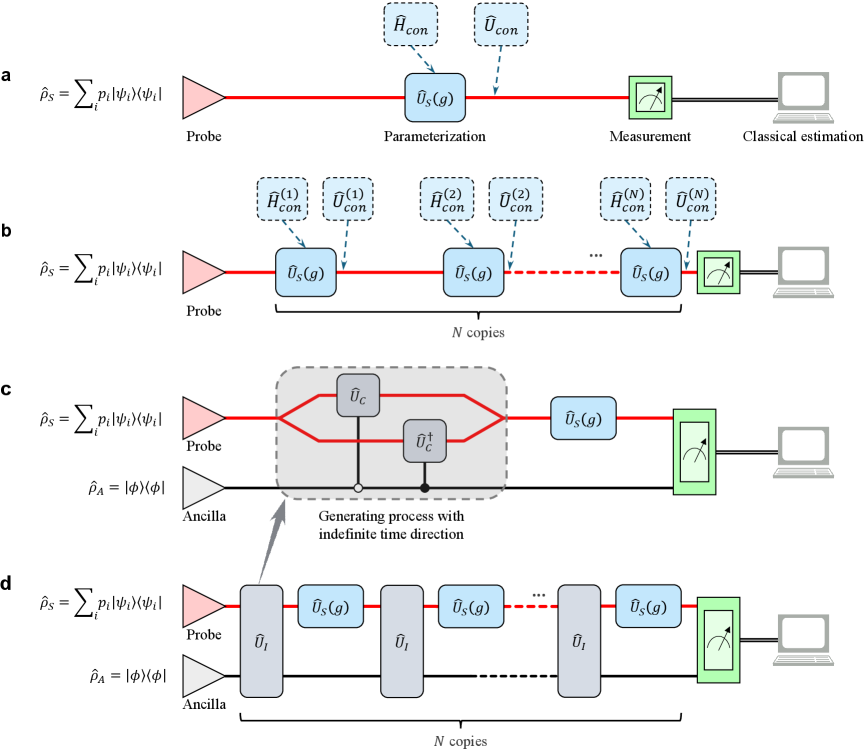
Figure 1: Schematic of quantum metrological schemes. a Standard quantum metrological scheme with a single-pass parameterizing process. $\hat{H}_{con}$ and $\hat{U}_{con}$ denotes the possible Hamiltonian and unitary controls applied to the probe state. b Standard quantum metrological scheme with the probe passing through the identical parameterizing process $N$ times sequentially. $\hat{H}_{con}^{(i)}$ and $\hat{U}_{con}^{(i)}$ denotes the possible Hamiltonian and unitary controls applied to the probe state during $i$-th parameterizing process. c Quantum metrological scheme with an ITD generating process. The Hamiltonian $\hat{H}_{C}$ of the generating process is conjugate to the characteristic operator $\hat{V}_{S}$ of the parameterizing process. The ancilla is a qubit to implement the quantum switch. d Quantum metrological scheme with the probe passing through the identical ITD generating process and parameterizing process $N$ times sequentially. Every ITD generating process is prior to every single parameterizing process.

To determine the conditions under which the precision limit exhibits linear scaling with respect to $T$ and $N$, and to develop a general framework for achieving nonlinear-scaling enhancements in $\Delta\bar{\mathcal{K}}$, we first consider a standard quantum metrological scheme without ancillas, as depicted in Fig. 1a. A probe state $\hat{\rho}_{S}=\sum_{i}p_{i}|\psi_{i}\rangle\langle\psi_{i}|$ is prepared as the initial probe state for the metrological task. By allowing this prepared probe state $\hat{\rho}_{S}$ to evolve under the parameterizing process $\hat{U}_{S}(g)$ described by a parameter-dependent Hamiltonian $\hat{H}_{S}(g)$ during a time $T_{S}$, we can derive that the corresponding canonical momentum operator (Heisenberg picture) in the parameter space is expressed as $\hat{\mathcal{K}}_{S}=\int_{0}^{T_{S}}\hat{U}_{S}^{\dagger}(0\to t)[\partial_{g}\hat{H}_{S}(g)]\hat{U}_{S}(0\to t)\mathrm{d}t$. This result links the momentum in the parameter space to the dynamical characteristics of the parameterizing process. We denote the dynamical characteristic operator of this process as $\hat{V}_{S}=\partial_{g}\hat{H}_{S}(g)$.

Conventionally, the eigenvalues of $\hat{H}_{S}$ or $\hat{V}_{S}$ are considered to be bounded in quantum metrology. Under this constraint, it is believed that the precision limit cannot beat the conventional Heisenberg scaling of $1/\mathcal{H}$ (i.e., linear scaling with respect to $T$ or $N$)[46, 47, 48] and that ancillas offer no advantage in noiseless settings[49]. However this constraint restricts consideration to finite-dimensional quantum systems, which is not applicable to many practical scenarios. In particular, quantum optical systems often exhibit inherently infinite-dimensional characteristics, such as continuous variables, orbital angular momentum (OAM), and spatial modes of photons are prevalent, making the constraint on eigenvalues impractical.

In contrast to the traditional consideration in previous works, we impose a constraint on the maximum average uncertainty of $\hat{V}_{S}$. The average uncertainty of $\hat{V}_{S}$ with respect to an arbitrary quantum state $\hat{\rho}_{S}=\sum_{i}p_{i}|\psi_{i}\rangle\langle\psi_{i}|$ in the Hilbert space of the probe state is defined as $\Delta\bar{V}_{S}^{2}=\sum_{i}p_{i}(\langle\psi_{i}|\hat{V}_{S}^{2}|\psi_{i}\rangle-\langle\psi_{i}|\hat{V}_{S}|\psi_{i}\rangle^{2})$. We constrain this average uncertainty $\Delta\bar{V}_{S}$ by a maximum value $\Delta\mathcal{V}_{S}$. Notably, this average uncertainty constraint on $\hat{V}_{S}$ is more applicable in quantum metrology than the conventional eigenvalue constraint, since it imposes a weaker constraint on systems and probes ($\Delta\bar{V}_{S}^{2}\leq\Delta V_{S}^{2}=\mathrm{Tr}(\hat{\rho}\hat{V}_{S}^{2})-\mathrm{Tr}(\hat{\rho}\hat{V}_{S})^{2}\leq V_{S}^{2}=\mathrm{Tr}(\hat{\rho}\hat{V}_{S}^{2})$)[50]. Importantly, it is applicable for both finite-dimensional and infinite-dimensional scenarios, thereby allowing for a more general conclusion in evaluating the scaling of precision limits. Subsequently, we can further establish that the uncertainty of the canonical momentum is then bounded by $\Delta\bar{\mathcal{K}}_{S}^{2}\leq T_{S}\int_{0}^{T_{S}}\Delta\mathcal{V}_{S}^{2}\,\mathrm{d}t=\Delta\mathcal{V}_{S}^{2}T_{S}^{2}$. (See the Supplemental Materials for the detailed proof.) This result leads to the linear Heisenberg limit

$${\delta g}_{S}\geq\frac{1}{2\sqrt{\nu}\Delta\mathcal{V}_{S}T},$$ (2)

where $T=T_{S}$ represents the evolution time of probe state.

Next, we allow the probe to pass through the identical parameterizing process $N$ times sequentially, as shown in Fig. 1b. The sequential evolution of the probe state can then be expressed as $\hat{U}_{S}^{(N)}=[\hat{U}_{S}(g)]^{N}$, then the corresponding canonical momentum in the Heisenberg picture can be calculated as $\hat{\mathcal{K}}_{S}^{(N)}=\mathrm{i}[\hat{U}_{S}^{(N)}]^{\dagger}[\partial_{g}\hat{U}_{S}^{(N)}]=\sum_{j=0}^{N-1}(\hat{U}_{S}^{\dagger})^{j}\hat{\mathcal{K}}_{S}(\hat{U}_{S})^{j}$. We can finally derive that the uncertainty of the canonical momentum $\hat{\mathcal{K}}_{S}^{(N)}$ is bounded by $[\Delta\bar{\mathcal{K}}_{S}^{(N)}]^{2}\leq N^{2}\Delta\mathcal{V}_{S}^{2}T_{S}^{2}$. (See the Supplemental Materials for the detailed proof.) Substituting this into Eq. (1), we can derive the ultimate precision limit of standard quantum metrological scheme with the probe passing through the identical parameterizing process $N$ times as (Here we normalize the time length of a single-shot parameterizing process as $T_{S}=1$.)

$${\delta g}_{S}^{(N)}\geq\frac{1}{2\sqrt{\nu}\Delta\mathcal{V}_{S}N},$$ (3)

which is a linear-scaling limit with respect to the iteration number $N$.

Consequently, in ancilla-free quantum metrological schemes, the ultimate precision limits exhibit, at most, linear scaling with respect to the total evolution time $T$ or the number of probes/quantum gates $N$, provided that the average uncertainty of the characteristic operator $\hat{V}_{S}$ is bounded. This conclusion holds not only for finite-dimensional systems but also extends to infinite-dimensional systems, even when optimal unitary or Hamiltonian controls are applied to the probes. These results indicate that, under such uncertainty constraint, achieving nonlinear-scaling precision limits in quantum metrology requires ancillas and advanced quantum resources. However, employing unbounded ancillas may incur additional energy costs. Notably, we find that the quantum switch constitutes a promising strategy, as it can incorporate underlying resources associated with noncommutativity and quantum superpositions in quantum metrology, utilizing a single external two-level ancilla.

Specifically, we devise a generating process with an indefinite time direction (ITD) prior to the parameterizing process, which shifts the probe state in opposite directions beforehand. The ITD generating process is implemented via a two-level ancilla, which serves as the quantum switch, as depicted in Fig. 1c. In our scheme, we focus on the parameterizing process governed by a time-independent Hamiltonian $\hat{H}_{S}$, which possess a time-independent characteristic operator $\hat{V}_{S}$, thereby ensuring the constraint on its average uncertainty throughout the evolution. The corresponding generating process with a definite time direction is realized by a unitary operator $\hat{U}_{C}=\exp(-\mathrm{i}\hat{H}_{C}T_{C})$, with evolution time $T_{C}$, where the Hamiltonian satisfies $[\hat{H}_{C},\hat{V}_{S}]=\pm\mathrm{i}$ and $[\hat{H}_{C},[\hat{H}_{C},\hat{H}_{S}]]=[\hat{H}_{S},[\hat{H}_{C},\hat{H}_{S}]]=0$ (without loss of generality, we take $[\hat{H}_{C},\hat{V}_{S}]=\mathrm{i}$ in this article). By employing a two-level ancilla $\hat{\rho}_{A}=|\phi\rangle\langle\phi|$ as a quantum switch, we can generate a coherent superposition of forward- and backward-time-direction evolutions for the probe state $\hat{\rho}_{S}$ during the ITD generating process. The unitary evolution of this ITD generating process can then be written as $\hat{U}_{I}=\hat{U}_{C}\otimes|0\rangle\langle 0|+\hat{U}_{C}^{\dagger}\otimes|1\rangle\langle 1|$. This process results in additional increment and decrement on the operator $\hat{V}_{S}$ with generating time $T_{C}$ regarding to different time directions. Given that the entire evolution of the generating process and the parameterizing process can be written as $\hat{U}_{IS}=\hat{U}_{S}\hat{U}_{C}\otimes|0\rangle\langle 0|+\hat{U}_{S}\hat{U}_{C}^{\dagger}\otimes|1\rangle\langle 1|$, the canonical momentum operator of the joint system of probe and ancilla is derived as $\hat{K}_{I}=\mathrm{i}(\partial_{g}\hat{U}_{IS})\hat{U}_{IS}^{\dagger}=\hat{K}_{S}\otimes\hat{\mathbb{I}}$. In the Heisenberg picture, this momentum operator evolves as $\hat{\mathcal{K}}_{I}=\hat{U}_{IS}^{\dagger}\hat{K}_{I}\hat{U}_{IS}$ after the entire evolution, which can be calculated as

$$\hat{\mathcal{K}}_{I}=\left(\hat{\mathcal{K}}_{S}-T_{C}T_{S}\right)\otimes|0\rangle\langle 0|+\left(\hat{\mathcal{K}}_{S}+T_{C}T_{S}\right)\otimes|1\rangle\langle 1|.$$ (4)

This result indicates that the additional increment (decrement) on the canonical momentum is proportional to the product of the generating time $T_{C}$ and the parameterizing time $T_{S}$, which is nonlinear with the entire evolution time $T_{C}+T_{S}$. Then the uncertainty of the canonical momentum operator can be calculated and is bounded by $\Delta\hat{\mathcal{K}}_{I}^{2}\leq\Delta\mathcal{V}_{S}^{2}T_{S}^{2}+T_{C}^{2}T_{S}^{2}$, which determines the ultimate precision limit in our scheme as

$${\delta g}_{I}\geq\frac{1}{2\sqrt{\nu}}\cdot\frac{1}{\sqrt{\Delta\mathcal{V}_{S}^{2}T^{2}+T^{4}}},$$ (5)

where we assign the time length of generating process as $T_{C}=T_{S}=T$ (which is the optimal setting when the total evolution time is fixed). This limit is achievable in practice by choosing the ancilla as the maximum superposition state. (refer to the Supplemental Materials.) Compared to the standard quantum metrological scheme, our approach requires doubling the total evolution time of the probe state due to an additional generating process. However, this linear increase in the total evolution time results in a nonlinear enhancement in the precision limit, which was previously believed to be the super-Heisenberg limit and unachievable with a time-independent Hamiltonian. Thus, our results reveal the inherent physical mechanism to achieve the nonlinear-scaling precision limit and its connection to the Heisenberg’s uncertainty principle.

Subsequently, we allow both the probe and the ancilla to pass through the identical ITD generating process and parameterizing process $N$ times sequentially, as depicted in Fig. 1d. The entire evolution of the joint system of the probe and ancilla can be denoted as $\hat{U}_{IS}^{(N)}=(\hat{U}_{S}\hat{U}_{C})^{N}\otimes|0\rangle\langle 0|+(\hat{U}_{S}\hat{U}_{C}^{\dagger})^{N}\otimes|1\rangle\langle 1|$. Therefore, the corresponding canonical momentum operator of the joint system (in the Heisenberg picture) can be derived as $\hat{\mathcal{K}}_{I}^{(N)}=\mathrm{i}[\hat{U}_{IS}^{(N)}]^{\dagger}[\partial_{g}\hat{U}_{IS}^{(N)}]=\sum_{j=0}^{N-1}(\hat{U}_{C}^{\dagger}\hat{U}_{S}^{\dagger})^{j}\hat{U}_{C}^{\dagger}\hat{\mathcal{K}}_{S}\hat{U}_{C}(\hat{U}_{S}\hat{U}_{C})^{j}\otimes|0\rangle\langle 0|+\sum_{j=0}^{N-1}(\hat{U}_{C}\hat{U}_{S}^{\dagger})^{j}\hat{U}_{C}\hat{\mathcal{K}}_{S}\hat{U}_{C}^{\dagger}(\hat{U}_{S}\hat{U}_{C}^{\dagger})^{j}\otimes|1\rangle\langle 1|$, which can be finally calculated as (see the Supplemental Materials for calculation details)

$$\hat{\mathcal{K}}_{I}^{(N)}=\left(\hat{\mathcal{K}}_{S}^{(N)}-\frac{N^{2}+N}{2}T_{C}T_{S}\right)\otimes|0\rangle\langle 0|+\left(\hat{\mathcal{K}}_{S}^{(N)}+\frac{N^{2}+N}{2}T_{C}T_{S}\right)\otimes|1\rangle\langle 1|.$$ (6)

This result indicates that the additional increment (decrement) on the canonical momentum increases quadratically with the iteration number $N$ of the metrological process in our quantum metrological scheme. Then we can derive that the uncertainty of the canonical momentum $\hat{\mathcal{K}}_{I}^{(N)}$ is bounded by $[\Delta\bar{\mathcal{K}}_{I}^{(N)}]^{2}\leq\Delta\mathcal{V}_{S}^{2}N^{2}T_{S}^{2}+(N^{2}+N)^{2}T_{C}^{2}T_{S}^{2}/4$, which leads to a nonlinear-scaling Heisenberg limit with respect to the iteration number $N$ of the metrological process

$${\delta g}_{I}^{(N)}\geq\frac{1}{\sqrt{\nu}}\cdot\frac{1}{\sqrt{4\Delta\mathcal{V}_{S}^{2}N^{2}+(N^{2}+N)^{2}}},$$ (7)

where we normalize the time lengths as $T_{C}=T_{S}=1$. This limit is achievable in practice by choosing the ancilla as the maximum superposition state. (refer to the Supplemental Materials.) The generating process modifies the canonical momentum of the system, possibly increasing the energy of the probe state. However, in quantum optical systems, many properties of photons, such as polarization, spatial mode, and OAM, do not involve real-world energies. By leveraging these properties of photons, we can achieve this nonlinear-scaling enhancement in precision limits without incurring additional energy costs in the probe state. This holds significant importance for the practical applications of quantum metrology.

II.2 Experiment

To demonstrate the nonlinear Heisenberg limit experimentally, we investigate a practical metrological scenario of angular rotation in the quantum optical system. In this scenario, the unitary evolution of the parameterizing process is given as $\hat{U}_{S}=\exp(-\mathrm{i}gT_{S}\hat{L}_{z})$, where $\hat{L}_{z}$ is the OAM operator of photons and $gT_{S}=\alpha$ is the rotation angle. In our experimental settings, we modulate different values of the rotation angle $\alpha$ on photons to achieve the desired values of the unknown parameter $g$ or the evolution time length $T_{S}$, assuming one of their values is fixed. Specifically, the evolution time length $T_{S}$ will be directly determined by the rotation angle $\alpha$ when the value of the unknown parameter $g$ is fixed as a constant, and vice versa. Therefore, the generating process ought to shift the OAM of photons, which can be designed as $\hat{U}_{C}=\exp(-\mathrm{i}T_{C}\hat{\varphi})$, wherein the evolution time length $T_{C}=m$ is the topological charge in practice and the angular position operator $\hat{\varphi}$ satisfies $[\hat{\varphi},\hat{L}_{z}]=\mathrm{i}$. This unitary evolution of the generating process introduces an extra spiral phase on the photons, thereby shifting the OAM of the photons by a value of $m$. Notably, the commutation relation $[\hat{\varphi},\hat{L}_{z}]=\mathrm{i}$ holds only when the domain of $\hat{\varphi}$ is restricted to any open interval within $[0,2\pi]$. This is because $\varphi$ is not differentiable at the boundaries of $[0,2\pi]$, so that $\hat{L}_{z}=-\mathrm{i}\partial_{\varphi}$ is not applicable at these points. As discussed in [51], this problem can be avoided by considering the functions $\cos\hat{\varphi}$ and $\sin\hat{\varphi}$ as basic observables, instead of $\hat{\varphi}$ itself, since the latter is not a good observable either classically or quantum theoretically. In our experimental scheme, we actually consider the commutation relation between the OAM operator $\hat{L}_{z}$ and the unitary operator $\hat{U}_{C}$, wherein $\mathrm{e}^{\mathrm{i}\hat{\varphi}}=\cos\hat{\varphi}+\mathrm{i}\sin\hat{\varphi}$ is taken as the basic observable. Thus, the complications associated with the discontinuity of the angle operator $\hat{\varphi}$ do not arise within our framework.

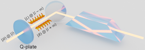
Figure 2: Experimental implementation of a single-shot evolution that includes an ITD generating process and a parameterizing process. A Q-plate and a mirror are used to shift the OAM of the probe in opposite directions for the different spin states $|R\rangle$ and $|L\rangle$. Rotating the Dove prism by an angle of $\alpha/2$ introduces a rotation angle of $\alpha$ on the profile of the photon beam.

In experiments, we use a Dove prism to implement the parameterizing process. It can rotate the transverse profile of photons, i.e., implement the unitary operator $\hat{U}_{S}=\exp(-\mathrm{i}\alpha\hat{L}_{z})$ on the probe states, by rotating the prism with a angle of $\alpha/2$. Here we employ OAM state $|\psi(l)\rangle$ of the photon as the probe state, where $\psi(l)$ denotes its wave function in the OAM representation. In our experiments, we initialize the probe state as a photon beam with a Gaussian-profile, corresponding to an OAM value of 0. Moreover, the spin state of photons is used as the ancilla, where the right-handed circular polarization state $|R\rangle$ and left-handed circular polarization state $|L\rangle$ are the orthogonal basis of ancilla. The spin state of ancilla is initialized as $|H\rangle=\frac{1}{\sqrt{2}}(|R\rangle+|L\rangle)$ in experiment, i.e., horizontal polarization state. To implement the generating process with an indefinite time direction, we employ the Q-plate in experiment, which introduces a pair of opposite OAM shifts on the probe state based on the spin state of photons. Specifically, the $m$-order Q-plate flips the spin state of ancilla, meanwhile shifts the OAM of the probe state by a value of $-m$ with right-handed spin $|R\rangle$ and a value of $m$ with left-handed spin $|L\rangle$. This process can be denoted as $\mathrm{e}^{-\mathrm{i}m\hat{\varphi}}\otimes|L\rangle\langle R|+\mathrm{e}^{\mathrm{i}m\hat{\varphi}}\otimes|R\rangle\langle L|$ mathematically. As depicted in Fig. 2, we insert a mirror between the Q-plate and Dove prism. In experiment, the reflection on mirror flips the spin state of photons and inverses the topological charge of probe state simultaneously, and the total internal reflection in Dove prism only inverses the topological charge of probe state. Therefore, a single-shot evolution comprising an ITD generating process and a parameterizing process can be denoted as $\mathrm{e}^{-\mathrm{i}\alpha\hat{L}_{z}}\mathrm{e}^{-\mathrm{i}m\hat{\varphi}}\otimes|R\rangle\langle R|+\mathrm{e}^{-\mathrm{i}\alpha\hat{L}_{z}}\mathrm{e}^{\mathrm{i}m\hat{\varphi}}\otimes|L\rangle\langle L|$ in experiment.

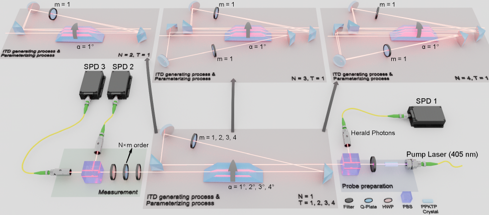
Figure 3: Experimental setup. The system comprises three main parts: Preparation of the probe state and ancilla state, joint evolution of the probe and the ancilla which includes the ITD generating process and the parameterizing process, measurement of the final state. The SPDC process in the PPKTP crystal converts a $405\text{\,}\mathrm{nm}$ photon into an $810\text{\,}\mathrm{nm}$ single-photon pair with orthogonal polarization. Idler photons are separated by a PBS to herald signal photons. The signal photon (zero OAM) serves as the probe, and its polarization state serves as the ancilla. Different Q-plate orders and Dove prism rotation angles implement various evolution times $T$. By adjusting right-angle prism mirrors, photons pass through the Q-plate and Dove prism multiple times, achieving various iteration numbers $N$. Projective measurement is conducted using a PBS, two HWPs, and an $N\times m$-order Q-plate. Photon numbers under orthogonal projections are detected via coincidence counting between SPD 2 and SPD 1, and between SPD 3 and SPD 1.

Fig. 3 delineates the configuration of our experimental apparatus. To initialize the probe and ancilla, we generate single-photon pairs through a degenerated type-II spontaneous parametric down-conversion (SPDC) process within a periodically poled potassium titanyl phosphate (PPKTP) crystal, pumped by a $405\text{\,}\mathrm{nm}$ continuous wave (cw) laser. Due to the SPDC process inside the PPKTP crystal, the single-photon pairs work at $810\text{\,}\mathrm{nm}$, then the signal photon and idler photon are separated by a polarizing beam splitter (PBS). Thus the polarization of the signal photon is initialized as $|H\rangle$. Although we initialize the probe state as a Gaussian-profile photon beam, our experiments do not rely on the OAM distribution of the probe state. For generality, we represent the initial state of the joint system of probe and ancilla as $|\psi(l)\rangle\otimes|H\rangle$. The idler photon is finally measured by a single photon detector (SPD) and serves as a trigger for the signal photon evolved through the experimental setup. In principle, a single-shot evolution, as depicted in Fig. 2, leads the probe and ancilla to the state $|\Psi_{f}\rangle=\frac{1}{\sqrt{2}}\mathrm{e}^{-\mathrm{i}\alpha\hat{L}_{z}}(|\psi(l-m)\rangle\otimes|R\rangle+|\psi(l+m)\rangle\otimes|L\rangle)$.

Fist, we fix the value of unknown parameter as $g=\pi/180$, thus various rotation angles $\alpha$ represents the distinct parameterizing evolution times $T_{S}$. Since rotation angle $\alpha=gT_{S}$, a rotation angle of $\alpha=$$$ corresponds to the normalized evolution time of $T_{S}=1$ in this case. Additionally, the evolution time $T_{C}$ of the generating process is represented by the order $m$ of the Q-plate ($T_{C}=m$), with $m=1$ corresponding to the normalized evolution time $T_{C}=1$. Here, we designate the dimensionless evolution time $T_{S}=T_{C}=T$. To estimate the unknown parameter from the final state, a practical projective measurement is devised for the experiment. As depicted in Fig. 3, a half-wave plate (HWP) followed by a $m$-order Q-plate are used to eliminate the topological charges on probe state. Theoretically, the HWP, with its optical axis set either parallel or perpendicular to the horizontal plane, flips the spin state of the photons. Consequently, the unitary evolution of this process, which comprises a HWP and an $m$-order Q-plate, can be represented as $\hat{U}_{m}=\mathrm{e}^{-\mathrm{i}m\hat{\varphi}}\otimes|L\rangle\langle L|+\mathrm{e}^{\mathrm{i}m\hat{\varphi}}\otimes|R\rangle\langle R|$. Subsequent to this, another HWP, with its optical axis set at an angle of $22.5\mathrm{°}$ to the horizontal plane, followed by a PBS, are employed to project the final state of ancilla onto the $45\mathrm{°}$ linearly polarized state $|+\rangle$ and the $-$$$ linearly polarized state $|-\rangle$. Given these configurations, the orthogonal projection operators performing on the final state can be represented as

$$\begin{split}\hat{\Pi}_{+}&=\hat{U}_{m}^{\dagger}\left(\hat{\mathbb{I}}\otimes|+\rangle\langle+|\right)\hat{U}_{m},\\ \hat{\Pi}_{-}&=\hat{U}_{m}^{\dagger}\left(\hat{\mathbb{I}}\otimes|-\rangle\langle-|\right)\hat{U}_{m}.\end{split}$$ (8)

Then we can calculate that

$$\hat{U}_{m}|\Psi_{f}\rangle =\mathrm{e}^{-\mathrm{i}\alpha\hat{L}_{z}}|\psi(l)\rangle\otimes\frac{1}{\sqrt{2}}\left(\mathrm{e}^{\mathrm{i}m\alpha}|R\rangle+\mathrm{e}^{-\mathrm{i}m\alpha}|L\rangle\right)$$

$$=\mathrm{e}^{-\mathrm{i}gT\hat{L}_{z}}|\psi(l)\rangle\otimes\frac{1}{\sqrt{2}}\left(\mathrm{e}^{\mathrm{i}gT^{2}}|R\rangle+\mathrm{e}^{-\mathrm{i}gT^{2}}|L\rangle\right),$$ (9)

wherein $T=T_{S}=\alpha/g=T_{C}=m$. Thus, the projective measurement is equivalent to applying the operators $|+\rangle\langle+|$ and $|-\rangle\langle-|$ to the final polarization state (ancilla) $|\phi_{f}\rangle=(\mathrm{e}^{\mathrm{i}gT^{2}}|R\rangle+\mathrm{e}^{-\mathrm{i}gT^{2}}|L\rangle)/\sqrt{2}$, which leads to the projective probabilities

$$\begin{split}P_{+}&=\langle\Psi_{f}|\hat{\Pi}_{+}|\Psi_{f}\rangle=\frac{1}{2}\left[1+\sin\left(2gT^{2}\right)\right],\\ P_{-}&=\langle\Psi_{f}|\hat{\Pi}_{-}|\Psi_{f}\rangle=\frac{1}{2}\left[1-\sin\left(2gT^{2}\right)\right].\end{split}$$ (10)

According to the classical parameter estimation theory, the experimental precision of estimating parameter $g$ is governed by the inequality

$$\delta g_{\mathrm{exp}}\geq\frac{1}{2\sqrt{\nu}T^{2}},$$ (11)

where $\nu$ is the number of independent measurements (the number of measured photons). This result is derived from the classical Cramér-Rao bound and Fisher information (see the Supplemental Materials for details).

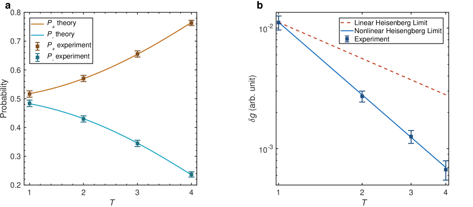
Figure 4: Experimental results with different dimensionless evolution time $T$. a Experimental results of the projective probabilities $P_{+}$ and $P_{-}$. The brown line and the cyan line represent the theoretical predictions of $P_{+}$ and $P_{-}$ calculating by Eq. (10), separately. The brown squares with error bars are the experimental results of $P_{+}$ and the cyan squares with error bar are the experimental results of $P_{-}$. b Experimental results of the RMSE of unknown parameter $g$. The solid blue line represents the nonlinear Heisenberg limit given by Eq. (11) and the dashed red line represent the linear Heisenberg limit of the standard quantum metrological scheme with the normalized maximum average uncertainty $\Delta\mathcal{V}_{S}=1$. The blue squares with error bars are the experimental results of the RMSE on estimating the unknown parameter $g$.

In the experiment, we perform the coincidence counting between SPD 1 and SPD 2 to get the photon number under the projection $\hat{\Pi}_{+}$, meanwhile perform the coincidence counting between SPD 1 and SPD 3 to get the photon number under the projection $\hat{\Pi}_{-}$. Subsequently, we estimate parameter $g$ from the detected photon numbers under these two projections and calculate the corresponding root-mean-square error (RMSE) from these estimates (for more details, refer to the Supplemental Materials). As shown in Fig.3, we first conduct the experiments of a single-shot evolution comprising an ITD generating process and a parameterizing process with a dimensionless evolution time $T$ of 1, 2, 3, and 4. Specifically, the different time lengths are achieved by rotating the photon profile with an angle $\alpha=$$$, $2\mathrm{°}$, $3\mathrm{°}$, and $4\mathrm{°}$ meanwhile choosing the topological order $m$ of the Q-plate as 1, 2, 3, and 4, separately. To record the experimental results, we establish the detection time span for each SPD at $50\text{\,}\mathrm{ms}$, and standardize the total detected photon count $\tilde{\nu}$ to approximately 2000, achieved by regulating the pump laser’s power. This experiment was replicated 600 times, accomplished by logging the counting events of each SPD continuously for $30\text{\,}\mathrm{s}$ and subsequently segregating them into 600 groups with time spans of $50\text{\,}\mathrm{ms}$. This enables the calculation of projective probabilities $P_{+}$ and $P_{-}$, as well as the estimated value $\tilde{g}$ of the unknown parameter $g$ for each experimental result group. Fig. 4a displays the experimental results of $P_{+}$ and $P_{-}$ with their respective error bars, and plots the theoretical results of Eq. (10) for comparison. Our experimental findings align well with the theoretical predictions. We then divide the 600 sets of experimental results into 20 groups, each containing 30 sets of results, and calculate the RMSE of the unknown parameter $g$ for each group. The results are illustrated in Fig. 4b, with error bars. For comparison, the theoretical precision limit of Eq. (11) is plotted using a solid line, and the linear Heisenberg limit of the standard quantum metrological scheme (where the uncertainty of the operator $\hat{V}_{S}$ is normalized as $\Delta\mathcal{V}_{S}=1$, then ${\delta g}_{S}=1/(2\sqrt{\nu}T)$) is plotted using a dashed line.

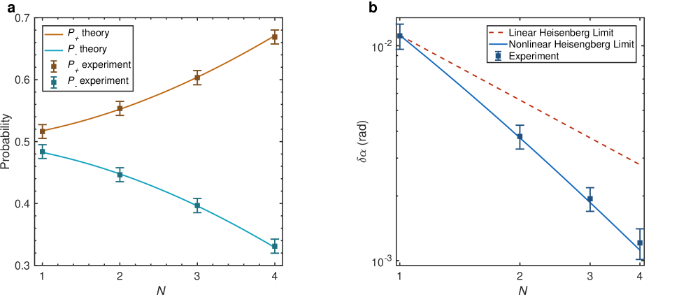
Figure 5: Experimental results in sequential strategy with $N$ copies of a single-shot evolution which comprises an ITD generating process and a parameterizing process. a Experimental results of the projective probabilities $P_{+}$ and $P_{-}$. The brown line and the cyan line represent the theoretical predictions of $P_{+}$ and $P_{-}$ calculating by Eq. (13), separately. The brown squares with error bars are the experimental results of $P_{+}$ and the cyan squares with error bar are the experimental results of $P_{-}$. b Experimental results of the RMSE of unknown parameter $\alpha$. The solid blue line represents the nonlinear Heisenberg limit given by Eq. (14) and the dashed red line represent the linear Heisenberg limit of the standard quantum metrological scheme with the normalized maximum average uncertainty $\Delta\mathcal{V}_{S}=1$. The blue squares with error bars are the experimental results of the RMSE on estimating the unknown parameter $\alpha$.

Subsequently, we sequentially apply the single-shot evolution, which comprises an ITD generating process and a parameterizing process, $N$ times to each probe (single photon). We here fix the value of the dimensionless evolution time as $T=T_{S}=T_{C}=1$, which means the topological order of the Q-plate is set to $m=1$ within our experimental settings. In this context, the unknown parameter $g$ is directly determined by the rotation angle $\alpha$ of the photon beam profile, i.e., $\alpha=gT=g$. Following the execution of $N$ iterations of a single-shot evolution process, we denote the final joint state of the probe and ancilla as $|\Psi_{f}^{(N)}\rangle$. We use experimental settings similar to those we’ve mentioned above to perform projective measurements on this final state, where an $N$-order Q-plate is employed in this case. Then the corresponding projective operators can be expressed as $\hat{\Pi}_{+}^{(N)}=\hat{U}_{N}^{\dagger}\left(\hat{\mathbb{I}}\otimes|+\rangle\langle+|\right)\hat{U}_{N}$ and $\hat{\Pi}_{-}^{(N)}=\hat{U}_{N}^{\dagger}\left(\hat{\mathbb{I}}\otimes|-\rangle\langle-|\right)\hat{U}_{N}$, where $\hat{U}_{N}=\mathrm{e}^{-\mathrm{i}N\hat{\varphi}}\otimes|L\rangle\langle L|+\mathrm{e}^{\mathrm{i}N\hat{\varphi}}\otimes|R\rangle\langle R|$. Similarly, we can calculate that

$$\hat{U}_{N}|\Psi_{f}^{(N)}\rangle=\mathrm{e}^{-\mathrm{i}N\alpha\hat{L}_{z}}|\psi(l)\rangle\otimes\frac{1}{\sqrt{2}}\left(\mathrm{e}^{\mathrm{i}\frac{N^{2}+N}{2}\alpha}|R\rangle+\mathrm{e}^{-\mathrm{i}\frac{N^{2}+N}{2}\alpha}|L\rangle\right),$$ (12)

wherein $\alpha=g$. The corresponding projective probabilities are then derived as

$$\begin{split}P_{+}^{(N)}&=\langle\Psi_{f}^{(N)}|\hat{\Pi}_{+}^{(N)}|\Psi_{f}^{(N)}\rangle=\frac{1}{2}\left\{1+\sin\left[(N^{2}+N)\alpha\right]\right\},\\ P_{-}^{(N)}&=\langle\Psi_{f}^{(N)}|\hat{\Pi}_{-}^{(N)}|\Psi_{f}^{(N)}\rangle=\frac{1}{2}\left\{1-\sin\left[(N^{2}+N)\alpha\right]\right\},\end{split}$$ (13)

which leads to the conclusion that the experimental precision in estimating parameter $g$ is governed by the inequality

$$\delta g_{\mathrm{exp}}^{(N)}=\delta\alpha\geq\frac{1}{\sqrt{\nu}(N^{2}+N)}.$$ (14)

We conduct the experiments of an iteration number $N$ of 1, 2, 3, and 4 by moving the right-angle prism mirrors in our experimental system, the corresponding experimental light paths are shown in the upper half part of Fig. 3. Similarly, we establish the detection time span for each SPD at $50\text{\,}\mathrm{ms}$, and standardize the total detected photon count $\tilde{\nu}$ to approximately 2000 to record the experimental results. This experiment was still replicated 600 times using the method we’ve mentioned above. We illustrate the experimental results of $P_{+}$ and $P_{-}$ with their respective error bars in Fig. 5a, and plot the theoretical results of Eq. (13) for comparison. Subsequently, we calculate the RMSE of the unknown parameter $\alpha$ by dividing the 600 sets of experimental results into 20 groups. The results are illustrated in Fig. 5b, with error bars. For comparison, the theoretical precision limit of Eq. (14) is plotted using a solid line, and the linear Heisenberg limit of the standard quantum metrological scheme (where the uncertainty of the operator $\hat{V}_{S}$ is normalized as $\Delta\mathcal{V}_{S}=1$, then $\delta\alpha=1/(2\sqrt{\nu}N)$) is plotted using a dashed line.

III Discussions

Conventionally, the quantum Cramér-Rao bound (QCRB) and the associated quantum Fisher information (QFI) are employed for evaluating the ultimate precision limit in quantum metrology[52]. Although in this work we derive the ultimate precision limit via the uncertainty relation in parameter space, the precision limit presented in Eq. (1) remains fully consistent with the QCRB framework (see Methods for a detailed proof). However, the QFI is directly determined by the symmetric logarithmic derivative (SLD) operator, which serves as the quantum counterpart to the classical logarithmic derivative in parameter estimation theory. While this formalism captures the statistical essence of the QFI, it does not provide direct insight into the underlying physical processes of the probe state in quantum metrology. On the contrary, our approach constructs the ultimate precision limit directly from the uncertainty relation in parameter space, fundamentally determined by the average momentum uncertainty on the probe state. In our framework, the canonical momentum $\hat{\mathcal{K}}$ is connected to the dynamical characteristics $\hat{V}_{S}=\partial_{g}\hat{H}_{S}$ of the parameterizing process. Consequently, unlike the conventional QFI-based approach, our perspective offers a more physically intuitive framework for investigating the relationship between the ultimate precision limit and the dynamics of the parameterizing process in quantum metrology.

Moreover, our uncertainty-principle-based approach reformulates the Heisenberg scaling as $1/\Delta\bar{\mathcal{K}}$, thereby unifying so-called “super-Heisenberg” limits within a common framework. The nonlinear-scaling precision limits observed in these scenarios fundamentally arise from nonlinear increases in the average uncertainty of the canonical momentum in the parameter space. We illustrate this unification by discussing three representative ”super-Heisenberg” regimes: nonlinear phase estimation[18, 19, 20], frequency estimation with a time-dependent Hamiltonian[21, 22] and geometric phase estimation under ICO[25, 26].

In nonlinear phase estimation, the canonical momentum $\hat{\mathcal{K}}$ is directly linked to the system’s energy. Here, pairwise photon-photon interactions for $N$ photons result in $N^{2}$ applications of phase encoding gates, corresponding to an system’s energy cost scaling of $1/N^{2}$—thereby enhancing the precision limit beyond the linear-scaling with respect to the number of photons.

For schemes involving time-dependent Hamiltonians, the application of time-dependent controls can induce an unbounded increase in the uncertainty of the operator $\hat{V}_{S}=\partial_{\omega}\hat{H}_{S}$ as the evolving time $T$ grows, where $\omega$ denotes the parameter to be estimated. In other words, this approach violates the maximum uncertainty constraint in our framework since it involves a time-dependent average uncertainty $\Delta\bar{V}_{S}\propto t$ that increases unboundedly with time, leading to a nonlinear increase in $\Delta\bar{\mathcal{K}}$ with respect to $T$.

In the ICO scenario, the geometric phase associated with the orthogonal phase-space displacements $\hat{X}$ and $\hat{P}$ is estimated. Then the canonical momentum $\hat{\mathcal{K}}$ is given by the Berry curvature $\mathrm{i}[\hat{X},\hat{P}]$. Inverting the causal order of $N$ $\hat{X}$ phase-space displacements and $N$ $\hat{P}$ phase-space displacements entails exchanging each $\hat{X}$ displacement with a $\hat{P}$ displacement $N$ times, which evidently increases the Berry curvature, and hence the canonical momentum, by a factor of $N^{2}$. Furthermore, employing a quantum switch, i.e., an indefinite causal order, converts this nonlinear increase in the canonical momentum into an increase in its uncertainty $\Delta\bar{\mathcal{K}}$. Consequently, the fundamental resources for achieving the nonlinear enhancement in this scenario arise from the noncommutativity of orthogonal phase-space displacements and the quantum superposition enabled by the quantum switch. These underlying quantum resources are failed to be accounted for with the traditional Heisenberg scaling $1/\mathcal{H}$, but are naturally incorporated within our reformulated scaling $1/\Delta\bar{\mathcal{K}}$.

Building on this analysis, together with our theoretical and experimental results, suggest that nonlinear-scaling enhancements in precision have thus far only been experimentally implemented in infinite-dimensional systems, provided that the evolving time $T$ and the applying number $N$ of parameterizing processes increase linearly, and average uncertainty of operator $\hat{V}_{S}=\partial_{g}\hat{H}_{S}$ is constrained. Although nonlinear-scaling enhancements have been realized in finite-dimensional systems via nonlinear interactions or time-dependent Hamiltonians, these rely on either a nonlinear increase in the number of quantum gates or an unbounded increase on average uncertainty of the operator $\hat{V}_{S}$. While we cannot definitively rule out the possibility of realizing nonlinear-scaling precision limits in finite-dimensional systems under these constraints, infinite-dimensional systems combined with quantum switch strategies appear to be more feasible and widely applicable in experimental quantum metrology for achieving nonlinear-scaling enhancements.

However, it is important to emphasize that, in our scheme, the observed scaling in precision limits does not originate directly from the infinite-dimensional property of the system itself. Rather, it is the generating process with ITD that plays a decisive role. Specifically, we have demonstrated that, in ancilla-free quantum metrological schemes, the Heisenberg scaling $1/\Delta\bar{\mathcal{K}}$ cannot surpass linear scaling with respect to $T$ and $N$ if the average uncertainty on $\hat{V}_{S}$ associate with the probe state is bounded–this holds for both finite- and infinite-dimensional systems. Additionally, we demonstrate that the ITD generating process we employed does not alter the average uncertainty on $\hat{V}_{S}$ associated with the probe state (see the Supplemental Materials for details). Fundamentally, the nonlinear-scaling enhancement in our scheme arises from the nonlinearly increased phase uncertainty on the ancilla, which leads to a nonlinear increment in $\Delta\bar{\mathcal{K}}$. This enhancement is essentially induced by the noncommutativity between the generating and parameterizing processes, as well as the indefinite time direction introduced by the quantum switch. These findings highlight the significance of quantum switch strategies, implemented with an extra ancilla, in enabling nonlinear-scaling enhancements in quantum metrology.

An important open question remains as to whether precision limits beyond the $1/N^{2}$ scaling can be achieved by employing more complex indefinite causal order or indefinite time direction schemes. In principle, it is possible that general strategies of indefinite causal order or indefinite time direction may offer enhancement scaling beyond $1/N^{2}$. However, as of now, only schemes based on the quantum switch–which leverage superpositions of causal orders or time directions–can be experimentally realized. These superposition-based schemes cannot offer scaling advantage beyond $1/N^{2}$[25, 26]. Therefore, the experimental realization of more general ICO and ITD strategies, as well as the exploration of precision limits surpassing the $1/N^{2}$ scaling, remain promising for future research.

IV Methods

IV.1 Experimental materials

We used a PPKTP crystal from Raicol Crystals with dimensions $\qtyproduct[product-units=power]{1x2x5}{}$. The Q-plates employed in our experiments were custom-made by LBTEK. To ensure that photons could traverse the Dove prism during each sequential evolution, we selected a Dove prism from Thorlabs with a transverse size of $\qtyproduct[product-units=power]{30x30}{}$. The Dove prism was mounted on a motorized goniometer equipped with a stepper motor to facilitate accurate rotation angles. Single-photon detection was carried out using Avalanche Photodiode (APD) detectors from LBTEK, operating in Geiger mode to amplify the signal of individual photons and output pulse signals to the event counter. The detected pulse signals from the three SPDs were input into the Moku:Pro from Liquid Instruments, which functioned as the event counter. An algorithm was developed to calculate the coincidence counts between SPD 2 and SPD 1, and between SPD 3 and SPD 1 from the logged timestamps provided by Moku:Pro (see Supplemental Materials for details on the algorithm).

IV.2 Heisenberg’s uncertainty relation between parameter and its canonical momentum

In the generalized quantum metrological scheme with a unitary parameterizing process $\hat{U}(g)$, the unitary operator $\hat{U}(g)$ maps a quantum state $\hat{\rho}=\sum_{i}p_{i}|\Psi_{i}\rangle\langle\Psi_{i}|$ in the Hilbert space $\mathbb{H}$ to a parameterized state $\hat{\rho}(g)=\hat{U}(g)\hat{\rho}\hat{U}^{\dagger}(g)=\sum_{i}p_{i}\hat{U}(g)|\Psi_{i}\rangle\langle\Psi_{i}|\hat{U}^{\dagger}(g)$ in the projective Hilbert space (parameter space) $\mathbb{H}/U(1)$. Here we denote the translation operator in the parameter space as $\hat{T}(g^{\prime})$, which shifts the parameterized state $\hat{\rho}(g)$ by a value of $g^{\prime}$, i.e., $\hat{T}(g^{\prime})\hat{U}(g)=\hat{U}(g+g^{\prime})$. Given that the operator $\hat{U}(g+g^{\prime})$ is unitary, we can known that the translation operator $\hat{T}(g^{\prime})$ is an unitary operator which satisfies $\hat{T}^{\dagger}(g^{\prime})\hat{T}(g^{\prime})=\hat{\mathbb{I}}$.

Beginning with the translation operator, we can define the canonical momentum in the parameter space. First, we define the infinitesimal generator of the translation in the parameter space as $\hat{K}=\mathrm{i}[\partial_{g^{\prime}}\hat{T}(g^{\prime})]_{\text{at $g^{\prime}=0$}}$, which is an Hermite operator. Then we can express the infinitesimal translation operator as $\hat{T}(\mathrm{d}g)=\hat{\mathbb{I}}-\mathrm{i}\hat{K}\mathrm{d}g+\mathrm{O}[(\mathrm{d}g)^{2}]$. Given that $\hat{T}(\mathrm{d}g)\hat{U}(g)=\hat{U}(g+\mathrm{d}g)$, we can derive that

$$\hat{U}(g)-\mathrm{i}\hat{K}\hat{U}(g)\mathrm{d}g =\hat{U}(g+\mathrm{d}g),$$

$$-\mathrm{i}\hat{K}\mathrm{d}g =\left[\hat{U}(g+\mathrm{d}g)-\hat{U}(g)\right]\hat{U}^{\dagger}(g).$$

Then the infinitesimal generator can be derived as

$$\hat{K}=\mathrm{i}[\partial_{g}\hat{U}(g)]\hat{U}^{\dagger}(g).$$

Subsequently, we investigate the commutator between the infinitesimal generator $\hat{K}$ and the position operator $\hat{g}$ in the parameter space to demonstrate that the operator $\hat{K}$ is exactly the canonical momentum in the parameter space. For the unitary operator $\hat{U}(g)$, we can calculate

$$\hat{T}(g^{\prime})\hat{g}\hat{U}(g)=\hat{T}(g^{\prime})g\hat{U}(g)=g\hat{U}(g+g^{\prime}),$$

while

$$\hat{g}\hat{T}(g^{\prime})\hat{U}(g)=\hat{g}\hat{U}(g+g^{\prime})=(g+g^{\prime})\hat{U}(g+g^{\prime}).$$

Therefore, we can first determine that the commutator between the translation operator and the position operator is

$$[\hat{g},\hat{T}(g^{\prime})]=g^{\prime}\hat{U}(g+g^{\prime})\hat{U}^{\dagger}(g)=g^{\prime}\hat{T}(g^{\prime}).$$ (15)

Next, we take the partial derivative with respect to $g^{\prime}$ on both sides of Eq. (15)

$$[\hat{g},\partial_{g^{\prime}}\hat{T}(g^{\prime})]=\hat{T}(g^{\prime})+g^{\prime}\partial_{g^{\prime}}\hat{T}(g^{\prime})$$

Given that the infinitesimal generator $\hat{K}=\mathrm{i}[\partial_{g^{\prime}}\hat{T}(g^{\prime})]_{\text{at $g^{\prime}=0$}}$, we can derive the commutator

$$[\hat{g},\hat{K}]=\mathrm{i},$$ (16)

which indicates that the infinitesimal generator $\hat{K}$ is the corresponding canonical momentum in the parameter space. Since $\hat{g}$ and $\hat{K}$ are two observables on the Hilbert space $\mathbb{H}$, the tightest uncertainty relation between these two observables on the parameterized state $\hat{\rho}(g)$ is described as[53, 54, 55]

$$\mathrm{Var}\left[\hat{\rho}(g),\hat{g}\right]\mathcal{F}\left[\hat{\rho}(g),\hat{K}\right]\geq\left|\mathrm{Tr}\left\{\hat{\rho}(g)[\hat{g},\hat{K}]\right\}\right|^{2},$$ (17)

where

$$\mathrm{Var}\left[\hat{\rho}(g),\hat{g}\right]=\mathrm{Tr}\left[\hat{\rho}(g)\hat{g}^{2}\right]-\mathrm{Tr}\left[\hat{\rho}(g)\hat{g}\right]^{2}$$

denotes the uncertainty of the unknown parameter $g$ on the parameterized state $\hat{\rho}(g)$, i.e., $\delta g=\sqrt{\mathrm{Var}\left[\hat{\rho}(g),\hat{g}\right]}$. While $\mathcal{F}\left[\hat{\rho}(g),\hat{K}\right]$ stands for the quantum Fisher information of the state $\hat{\rho}(g)$ with respect to the observable $\hat{K}$, it can be calculated as[56, 55, 52]

$$\mathcal{F}\left[\hat{\rho}(g),\hat{K}\right] =2\sum_{i,j}\frac{(p_{i}-p_{j})^{2}}{p_{i}+p_{j}}\left|\langle\Psi_{i}|\hat{U}^{\dagger}(g)\hat{K}\hat{U}(g)|\Psi_{j}\rangle\right|^{2}$$

$$=2\sum_{i,j}\frac{(p_{i}-p_{j})^{2}}{p_{i}+p_{j}}\left|\langle\Psi_{i}|\hat{\mathcal{K}}|\Psi_{j}\rangle\right|^{2}$$

$$=\mathcal{F}\left[\hat{\rho},\hat{\mathcal{K}}\right],$$

where $\hat{\mathcal{K}}=\hat{U}^{\dagger}(g)\hat{K}\hat{U}(g)$ is the canonical momentum in the Heisenberg picture. We can further calculate $\mathcal{F}\left[\hat{\rho},\hat{\mathcal{K}}\right]$ as

$$\mathcal{F}\left[\hat{\rho},\hat{\mathcal{K}}\right] =2\sum_{i,j}(p_{i}+p_{j})\left|\langle\Psi_{i}|\hat{\mathcal{K}}|\Psi_{j}\rangle\right|^{2}-\sum_{i,j}\frac{8p_{i}p_{j}}{p_{i}+p_{j}}\left|\langle\Psi_{i}|\hat{\mathcal{K}}|\Psi_{j}\rangle\right|^{2}$$

$$=\sum_{i}4p_{i}\left(\langle\Psi_{i}|\hat{\mathcal{K}}^{2}|\Psi_{i}\rangle-\langle\Psi_{i}|\hat{\mathcal{K}}|\Psi_{i}\rangle^{2}\right)-\sum_{i\neq j}\frac{8p_{i}p_{j}}{p_{i}+p_{j}}\left|\langle\Psi_{i}|\hat{\mathcal{K}}|\Psi_{j}\rangle\right|^{2}$$

$$\leq\sum_{i}4p_{i}\left(\langle\Psi_{i}|\hat{\mathcal{K}}^{2}|\Psi_{i}\rangle-\langle\Psi_{i}|\hat{\mathcal{K}}|\Psi_{i}\rangle^{2}\right)$$

$$=4\Delta\bar{\mathcal{K}}^{2},$$

where $\Delta\bar{\mathcal{K}}=\sqrt{\sum_{i}p_{i}(\langle\Psi_{i}|\hat{\mathcal{K}}^{2}|\Psi_{i}\rangle-\langle\Psi_{i}|\hat{\mathcal{K}}|\Psi_{i}\rangle^{2})}$ denotes the average uncertainty of the initial quantum state $\hat{\rho}$ with respect to the observable $\hat{\mathcal{K}}$. Substituting above results into Eq. (17) and combining with Eq. (16), we can construct the uncertainty relation between the unknown parameter $g$ and its canonical momentum $\hat{\mathcal{K}}$ in the parameter space as

$$\delta g\Delta\bar{\mathcal{K}}\geq\frac{1}{2},$$ (18)

which means that the precision on estimating parameter $g$ from the parameterized state $\hat{\rho}(g)=\hat{U}(g)\hat{\rho}\hat{U}^{\dagger}(g)$ is governed by the average uncertainty of the initial state $\hat{\rho}$ with respect to the canonical momentum $\hat{\mathcal{K}}$. Furthermore, we prepare $\nu$ copies of the initial probe and let them go through the parameterizing process independently, then the ultimate precision limit on estimating parameter $g$ can be given as the result in Eq. (1).

Notably, when the initial quantum state is a pure state, i.e., $\hat{\rho}=|\Psi\rangle\langle\Psi|$, the uncertainty relation in Eq. (18) simplifies to the well-known Heisenberg uncertainty relation between position and momentum

$$\delta g\Delta\mathcal{K}\geq\frac{1}{2},$$

where $\Delta\mathcal{K}=\sqrt{\langle\Psi|\hat{\mathcal{K}}^{2}|\Psi\rangle-\langle\Psi|\hat{\mathcal{K}}|\Psi\rangle^{2}}$ denotes the uncertainty of the pure quantum state $|\Psi\rangle$ with respect to the canonical momentum $\hat{\mathcal{K}}$.

IV.3 Consistency with QCRB framework

In this section, we demonstrate the consistency between the precision limit presented in Eq. (1) and the QCRB framework.

Within QCRB framework, the ultimate precision limit is determined by the QFI. Theoretically, the QFI of an unknown parameter $g$ associated with a parameterized state $\hat{\rho}(g)$ is defined as $\mathcal{F}(g|\hat{\rho}(g))=\mathrm{Tr}[\hat{\rho}(g)\hat{L}_{g}^{2}]$, where $\hat{L}_{g}$ is the SLD operator with respect to $g$. The SLD operator is determined by the equation $\partial_{g}\hat{\rho}(g)=[\hat{\rho}(g)\hat{L}_{g}+\hat{L}_{g}\hat{\rho}(g)]/2$. Then the QFI can be further calculated as

$$\mathcal{F}\left[g|\hat{\rho}(g)\right]=2\sum_{i,j}\frac{1}{\lambda_{i}+\lambda_{j}}\left|\langle\lambda_{i}|\partial_{g}\hat{\rho}(g)|\lambda_{j}\rangle\right|^{2},$$ (19)

where $\hat{\rho}(g)=\sum_{i}\lambda_{i}|\lambda_{i}\rangle\langle\lambda_{i}|$ is the spectral decomposition of the parameterized quantum state $\hat{\rho}(g)$. In our work, we consider that the final state $\hat{\rho}(g)$ is parameterized through a unitary process $\hat{U}(g)$, and the initial quantum state is denoted as $\hat{\rho}=\sum_{i}p_{i}|\Psi_{i}\rangle\langle\Psi_{i}|$. Thus, the parameterized quantum state in our case is expressed as $\hat{\rho}(g)=\hat{U}(g)\hat{\rho}\hat{U}^{\dagger}(g)=\sum_{i}p_{i}\hat{U}(g)|\Psi_{i}\rangle\langle\Psi_{i}|\hat{U}^{\dagger}(g)$. Therefore, the eigenstate $|\lambda_{i}\rangle$ in $\hat{\rho}(g)$ can be written as $|\lambda_{i}\rangle=\hat{U}(g)|\Psi_{i}$, and the corresponding eigenvalue $\lambda_{i}=p_{i}$, which is parameter-independent. Then substituting these results into Eq. (19), we can calculate the QFI as:

$$\mathcal{F}\left[g|\hat{\rho}(g)\right]=2\sum_{i,j}\frac{1}{p_{i}+p_{j}}\left|p_{j}\langle\Psi_{i}|\hat{U}^{\dagger}(\partial_{g}\hat{U})|\Psi_{j}\rangle+p_{i}\langle\Psi_{i}|(\partial_{g}\hat{U}^{\dagger})\hat{U}|\Psi_{j}\rangle\right|^{2}.$$ (20)

In our theoretical scheme, the canonical momentum operator in the parameter space (in the Heisenberg picture) is given as $\hat{\mathcal{K}}=\mathrm{i}\hat{U}^{\dagger}(g)[\partial_{g}\hat{U}(g)]$, then the result in Eq. (20) can be further derived as

$$\mathcal{F}\left[g|\hat{\rho}(g)\right] =2\sum_{i,j}\frac{1}{p_{i}+p_{j}}\left|-\mathrm{i}p_{j}\langle\Psi_{i}|\hat{\mathcal{K}}|\Psi_{j}\rangle+\mathrm{i}p_{i}\langle\Psi_{i}|\hat{\mathcal{K}}|\Psi_{j}\rangle\right|^{2}$$

$$=2\sum_{i,j}\frac{(p_{i}-p_{j})^{2}}{p_{i}+p_{j}}\left|\langle\Psi_{i}|\hat{\mathcal{K}}|\Psi_{j}\rangle\right|^{2}$$

$$=\mathcal{F}\left[\hat{\rho},\hat{\mathcal{K}}\right],$$

which means that the QFI of the unknown parameter $g$ associated with the parameterized quantum state $\hat{\rho}(g)$ equals to the QFI of the observable $\hat{\mathcal{K}}$ associated with the initial quantum state $\hat{\rho}$. Since we have proved that $\mathcal{F}[\hat{\rho},\hat{\mathcal{K}}]\leq 4\Delta\bar{\mathcal{K}}^{2}$, our result $4\Delta\bar{\mathcal{K}}^{2}$ gives an upper bound of QFI and the “=” holds when $\langle\Psi_{i}|\hat{\mathcal{K}}|\Psi_{j}\rangle=0$ for $i\neq j$. Consequently, our result in Eq. (1) is fully consistent with the ultimate precision limit given by the QCRB, and it can be attained by employing the optimal probe state $\hat{\rho}=\sum_{i}p_{i}|\Psi_{i}\rangle\langle\Psi_{i}|$, where $\langle\Psi_{i}|\hat{\mathcal{K}}|\Psi_{j}\rangle=0$ for $i\neq j$.

Data and Materials Availability All data needed to evaluate the conclusions in the paper are present in the paper and the Supplementary Materials.

Competing Interests All authors declare that they have no competing interests.

Author Contribution

References

- Abadie et al. [2011] J. Abadie, B. P. Abbott, R. Abbott, T. D. Abbott, M. Abernathy, C. Adams, R. Adhikari, C. Affeldt, B. Allen, G. S. Allen, E. Amador Ceron, D. Amariutei, R. S. Amin, S. B. Anderson, W. G. Anderson, K. Arai, M. A. Arain, M. C. Araya, S. M. Aston, D. Atkinson, P. Aufmuth, C. Aulbert, B. E. Aylott, S. Babak, P. Baker, S. Ballmer, D. Barker, B. Barr, P. Barriga, L. Barsotti, M. A. Barton, I. Bartos, R. Bassiri, M. Bastarrika, J. Batch, J. Bauchrowitz, B. Behnke, A. S. Bell, I. Belopolski, M. Benacquista, J. M. Berliner, A. Bertolini, J. Betzwieser, N. Beveridge, P. T. Beyersdorf, I. A. Bilenko, G. Billingsley, J. Birch, R. Biswas, E. Black, J. K. Blackburn, L. Blackburn, D. Blair, B. Bland, O. Bock, T. P. Bodiya, C. Bogan, R. Bondarescu, R. Bork, M. Born, S. Bose, P. R. Brady, V. B. Braginsky, J. E. Brau, J. Breyer, D. O. Bridges, M. Brinkmann, M. Britzger, A. F. Brooks, D. A. Brown, A. Brummitt, A. Buonanno, J. Burguet-Castell, O. Burmeister, R. L. Byer, L. Cadonati, J. B. Camp, P. Campsie, J. Cannizzo, K. Cannon, J. Cao, C. D. Capano, S. Caride, S. Caudill, M. Cavagliá, C. Cepeda, T. Chalermsongsak, E. Chalkley, P. Charlton, S. Chelkowski, Y. Chen, N. Christensen, H. Cho, S. S. Y. Chua, S. Chung, C. T. Y. Chung, G. Ciani, F. Clara, D. E. Clark, J. Clark, et al., A gravitational wave observatory operating beyond the quantum shot-noise limit, Nature Physics 7, 962 (2011).
- Tse et al. [2019] M. Tse, H. Yu, et al., Quantum-enhanced advanced ligo detectors in the era of gravitational-wave astronomy, Phys. Rev. Lett. 123, 231107 (2019).
- Abe et al. [2021] M. Abe, P. Adamson, et al., Matter-wave atomic gradiometer interferometric sensor (magis-100), Quantum Science and Technology 6, 044003 (2021).
- Ludlow et al. [2015] A. D. Ludlow, M. M. Boyd, J. Ye, E. Peik, and P. O. Schmidt, Optical atomic clocks, Rev. Mod. Phys. 87, 637 (2015).
- Bongs et al. [2019] K. Bongs, M. Holynski, J. Vovrosh, P. Bouyer, G. Condon, E. Rasel, C. Schubert, W. P. Schleich, and A. Roura, Taking atom interferometric quantum sensors from the laboratory to real-world applications, Nature Reviews Physics 1, 731 (2019).
- Bennett et al. [2021] J. S. Bennett, B. E. Vyhnalek, H. Greenall, E. M. Bridge, F. Gotardo, S. Forstner, G. I. Harris, F. A. Miranda, and W. P. Bowen, Precision magnetometers for aerospace applications: A review, Sensors 21, 10.3390/s21165568 (2021).
- Hsiao et al. [2016] W. W.-W. Hsiao, Y. Y. Hui, P.-C. Tsai, and H.-C. Chang, Fluorescent nanodiamond: A versatile tool for long-term cell tracking, super-resolution imaging, and nanoscale temperature sensing, Accounts of Chemical Research 49, 400 (2016), pMID: 26882283, https://doi.org/10.1021/acs.accounts.5b00484 .
- Aslam et al. [2023] N. Aslam, H. Zhou, E. K. Urbach, M. J. Turner, R. L. Walsworth, M. D. Lukin, and H. Park, Quantum sensors for biomedical applications, Nature Reviews Physics 5, 157 (2023).
- Giovannetti et al. [2004] V. Giovannetti, S. Lloyd, and L. Maccone, Quantum-enhanced measurements: beating the standard quantum limit, Science 306, 1330 (2004), giovannetti, Vittorio Lloyd, Seth Maccone, Lorenzo eng Science. 2004 Nov 19;306(5700):1330-6. doi: 10.1126/science.1104149.
- Giovannetti et al. [2006] V. Giovannetti, S. Lloyd, and L. Maccone, Quantum metrology, Phys. Rev. Lett. 96, 010401 (2006).
- Giovannetti et al. [2011] V. Giovannetti, S. Lloyd, and L. Maccone, Advances in quantum metrology, Nature Photonics 5, 222 (2011).
- Yuan and Fung [2015] H. Yuan and C.-H. F. Fung, Optimal feedback scheme and universal time scaling for hamiltonian parameter estimation, Phys. Rev. Lett. 115, 110401 (2015).
- Rarity et al. [1990] J. G. Rarity, P. R. Tapster, E. Jakeman, T. Larchuk, R. A. Campos, M. C. Teich, and B. E. A. Saleh, Two-photon interference in a mach-zehnder interferometer, Phys. Rev. Lett. 65, 1348 (1990).
- Mitchell et al. [2004] M. W. Mitchell, J. S. Lundeen, and A. M. Steinberg, Super-resolving phase measurements with a multiphoton entangled state, Nature 429, 161 (2004).
- Afek et al. [2010] I. Afek, O. Ambar, and Y. Silberberg, High-noon states by mixing quantum and classical light, Science 328, 879 (2010), https://www.science.org/doi/pdf/10.1126/science.1188172 .
- Liu and Yuan [2017] J. Liu and H. Yuan, Quantum parameter estimation with optimal control, Phys. Rev. A 96, 012117 (2017).
- Hou et al. [2019] Z. Hou, R.-J. Wang, J.-F. Tang, H. Yuan, G.-Y. Xiang, C.-F. Li, and G.-C. Guo, Control-enhanced sequential scheme for general quantum parameter estimation at the heisenberg limit, Phys. Rev. Lett. 123, 040501 (2019).
- Boixo et al. [2007] S. Boixo, S. T. Flammia, C. M. Caves, and J. Geremia, Generalized limits for single-parameter quantum estimation, Phys. Rev. Lett. 98, 090401 (2007).
- Roy and Braunstein [2008] S. M. Roy and S. L. Braunstein, Exponentially enhanced quantum metrology, Phys. Rev. Lett. 100, 220501 (2008).
- Napolitano et al. [2011] M. Napolitano, M. Koschorreck, B. Dubost, N. Behbood, R. J. Sewell, and M. W. Mitchell, Interaction-based quantum metrology showing scaling beyond the heisenberg limit, Nature 471, 486 (2011), napolitano, M Koschorreck, M Dubost, B Behbood, N Sewell, R J Mitchell, M W eng Research Support, Non-U.S. Gov’t England Nature. 2011 Mar 24;471(7339):486-9. doi: 10.1038/nature09778.
- Pang and Jordan [2017] S. Pang and A. N. Jordan, Optimal adaptive control for quantum metrology with time-dependent hamiltonians, Nat Commun 8, 14695 (2017).
- Hou et al. [2021] Z. Hou, Y. Jin, H. Chen, J.-F. Tang, C.-J. Huang, H. Yuan, G.-Y. Xiang, C.-F. Li, and G.-C. Guo, “super-heisenberg” and heisenberg scalings achieved simultaneously in the estimation of a rotating field, Phys. Rev. Lett. 126, 070503 (2021).
- Yang [2019] Y. Yang, Memory effects in quantum metrology, Phys. Rev. Lett. 123, 110501 (2019).
- Altherr and Yang [2021] A. Altherr and Y. Yang, Quantum metrology for non-markovian processes, Phys. Rev. Lett. 127, 060501 (2021).
- Zhao et al. [2020] X. Zhao, Y. Yang, and G. Chiribella, Quantum metrology with indefinite causal order, Phys. Rev. Lett. 124, 190503 (2020).
- Yin et al. [2023] P. Yin, X. Zhao, Y. Yang, Y. Guo, W.-H. Zhang, G.-C. Li, Y.-J. Han, B.-H. Liu, J.-S. Xu, G. Chiribella, G. Chen, C.-F. Li, and G.-C. Guo, Experimental super-heisenberg quantum metrology with indefinite gate order, Nature Physics 10.1038/s41567-023-02046-y (2023).
- Zwierz et al. [2010] M. Zwierz, C. A. Pérez-Delgado, and P. Kok, General optimality of the heisenberg limit for quantum metrology, Phys. Rev. Lett. 105, 180402 (2010).
- Tsang [2012] M. Tsang, Ziv-zakai error bounds for quantum parameter estimation, Phys. Rev. Lett. 108, 230401 (2012).
- Giovannetti and Maccone [2012] V. Giovannetti and L. Maccone, Sub-heisenberg estimation strategies are ineffective, Phys. Rev. Lett. 108, 210404 (2012).
- Hall and Wiseman [2012] M. J. W. Hall and H. M. Wiseman, Does nonlinear metrology offer improved resolution? answers from quantum information theory, Phys. Rev. X 2, 041006 (2012).
- Pezzé [2013] L. Pezzé, Sub-heisenberg phase uncertainties, Phys. Rev. A 88, 060101 (2013).
- Rams et al. [2018] M. M. Rams, P. Sierant, O. Dutta, P. Horodecki, and J. Zakrzewski, At the limits of criticality-based quantum metrology: Apparent super-heisenberg scaling revisited, Phys. Rev. X 8, 021022 (2018).
- Helstrom [1973] C. W. Helstrom, Cramér-rao inequalities for operator-valued measures in quantum mechanics, International Journal of Theoretical Physics 8, 361 (1973).
- Braunstein et al. [1996] S. L. Braunstein, C. M. Caves, and G. Milburn, Generalized uncertainty relations: Theory, examples, and lorentz invariance, Annals of Physics 247, 135 (1996).
- Holevo [2011] A. Holevo, Probabilistic and Statistical Aspects of Quantum Theory (Edizioni della Normale, Pisa, 2011) pp. 219–264.
- Zwierz et al. [2012] M. Zwierz, C. A. Pérez-Delgado, and P. Kok, Ultimate limits to quantum metrology and the meaning of the heisenberg limit, Phys. Rev. A 85, 042112 (2012).
- Chiribella and Liu [2022] G. Chiribella and Z. Liu, Quantum operations with indefinite time direction, Communications Physics 5, 190 (2022).
- Guo et al. [2024] Y. Guo, Z. Liu, H. Tang, X.-M. Hu, B.-H. Liu, Y.-F. Huang, C.-F. Li, G.-C. Guo, and G. Chiribella, Experimental demonstration of input-output indefiniteness in a single quantum device, Phys. Rev. Lett. 132, 160201 (2024).
- Strömberg et al. [2024] T. Strömberg, P. Schiansky, M. T. Quintino, M. Antesberger, L. A. Rozema, I. Agresti, i. c. v. Brukner, and P. Walther, Experimental superposition of a quantum evolution with its time reverse, Phys. Rev. Res. 6, 023071 (2024).
- Xia et al. [2024] B. Xia, J. Huang, H. Li, Z. Luo, and G. Zeng, Nanoradian-scale precision in light rotation measurement via indefinite quantum dynamics, Science Advances 10, eadm8524 (2024), https://www.science.org/doi/pdf/10.1126/sciadv.adm8524 .
- Xia et al. [2020] B. Xia, J. Huang, C. Fang, H. Li, and G. Zeng, High-precision multiparameter weak measurement with hermite-gaussian pointer, Phys. Rev. Appl. 13, 034023 (2020).
- Xia et al. [2022] B. Xia, J. Huang, H. Li, M. Liu, T. Xiao, C. Fang, and G. Zeng, Ultrasensitive measurement of angular rotations via a hermite-gaussian pointer, Photon. Res. 10, 2816 (2022).
- Xia et al. [2023] B. Xia, J. Huang, H. Li, H. Wang, and G. Zeng, Toward incompatible quantum limits on multiparameter estimation, Nature Communications 14, 1021 (2023).
- Cimini et al. [2023] V. Cimini, E. Polino, F. Belliardo, F. Hoch, B. Piccirillo, N. Spagnolo, V. Giovannetti, and F. Sciarrino, Experimental metrology beyond the standard quantum limit for a wide resources range, npj Quantum Information 9, 10.1038/s41534-023-00691-y (2023).
- D’Ambrosio et al. [2013] V. D’Ambrosio, N. Spagnolo, L. Del Re, S. Slussarenko, Y. Li, L. C. Kwek, L. Marrucci, S. P. Walborn, L. Aolita, and F. Sciarrino, Photonic polarization gears for ultra-sensitive angular measurements, Nature Communications 4, 2432 (2013).
- Górecki et al. [2020] W. Górecki, R. Demkowicz-Dobrzański, H. M. Wiseman, and D. W. Berry, -corrected heisenberg limit, Phys. Rev. Lett. 124, 030501 (2020).
- Wan and Lasenby [2022] K. Wan and R. Lasenby, Bounds on adaptive quantum metrology under markovian noise, Phys. Rev. Res. 4, 033092 (2022).
- Kurdziałek et al. [2023] S. Kurdziałek, W. Górecki, F. Albarelli, and R. Demkowicz-Dobrzański, Using adaptiveness and causal superpositions against noise in quantum metrology, Phys. Rev. Lett. 131, 090801 (2023).
- Demkowicz-Dobrzański and Maccone [2014] R. Demkowicz-Dobrzański and L. Maccone, Using entanglement against noise in quantum metrology, Phys. Rev. Lett. 113, 250801 (2014).
- Hofmann and Takeuchi [2003] H. F. Hofmann and S. Takeuchi, Violation of local uncertainty relations as a signature of entanglement, Phys. Rev. A 68, 032103 (2003).
- Kastrup [2006] H. A. Kastrup, Quantization of the canonically conjugate pair angle and orbital angular momentum, Phys. Rev. A 73, 052104 (2006).
- Liu et al. [2019] J. Liu, H. Yuan, X.-M. Lu, and X. Wang, Quantum fisher information matrix and multiparameter estimation, Journal of Physics A: Mathematical and Theoretical 53, 023001 (2019).
- Pezzé and Smerzi [2009] L. Pezzé and A. Smerzi, Entanglement, nonlinear dynamics, and the heisenberg limit, Phys. Rev. Lett. 102, 100401 (2009).
- Fröwis et al. [2015] F. Fröwis, R. Schmied, and N. Gisin, Tighter quantum uncertainty relations following from a general probabilistic bound, Phys. Rev. A 92, 012102 (2015).
- Tóth and Fröwis [2022] G. Tóth and F. Fröwis, Uncertainty relations with the variance and the quantum fisher information based on convex decompositions of density matrices, Phys. Rev. Res. 4, 013075 (2022).
- Braunstein and Caves [1994] S. L. Braunstein and C. M. Caves, Statistical distance and the geometry of quantum states, Phys. Rev. Lett. 72, 3439 (1994).