A Morphology-Adaptive Random Feature Method for Inverse Source Problem of the Helmholtz Equation

Abstract

The inverse source problem for the Helmholtz equation poses significant challenges, particularly when sources exhibit complex or discontinuous geometries. Traditional numerical methods suffer from prohibitive computational costs, while machine learning-based approaches such as Physics-Informed Neural Networks (PINNs) and the Random Feature Method (RFM)—though computationally efficient for inverse problems—lack the intrinsic machinery to handle the sharp morphological features in such singular problems, leading to inaccurate solutions. To address this issue, we propose the Morphology-Adaptive Random Feature Method (MA-RFM), a novel two-phase framework that adaptively locates critical regions and adds morphology activation functions for tackling the multi-frequency inverse source problem with complex geometry. Our framework recasts the ill-posed inverse problem into a well-posed, strictly convex optimization problem by reformulating the governing Helmholtz equation as a Tikhonov-regularized integral equation via its fundamental solution. In the first stage, the Integral Adaptive RFM (IA-RFM), employs an adaptive algorithm to rapidly localize the source support, thereby reducing computational overhead and accelerating convergence. In the second stage, posterior geometric information is progressively integrated into the solver via hybrid basis functions, enabling a precise reconstruction of complex morphologies. The MA-RFM extends the capabilities of RFM to handle PDEs with singular solutions while preserving its mesh-free efficiency. We demonstrate the superior performance of our approach through ample challenging 2D and 3D benchmark problems, even under limited and noisy measurement conditions, highlighting its robustness and accuracy in reconstructing complex and disjoint sources.

Keywords: Helmholtz equation, inverse source problems, random feature method, morphology-adaptive basis, iterative adaptive integral mesh, multi-frequency.

1 Introduction

The inverse source problem of identifying an unknown scalar source in the Helmholtz equation arises in applications such as medical imaging, antenna synthesis, acoustic tomography, and pollution of the environment [1, 2, 3, 4, 5, 6, 7, 8, 9]. In this work, we consider the homogeneous Helmholtz equation. Let $\Omega$ be a bounded domain in $\mathbb{R}^{d}$, with boundary $\Gamma$. Assume that the source function $S(\bm{x})$ is compactly supported with support $\tau\subset\Omega\subset\subset\mathbb{R}^{d}$, which means $\mathrm{dist}(\tau,\Gamma):=\operatorname*{min}\{|\bm{x}-\bm{y}|{:}\ \bm{x}\in\tau,\bm{y}\in\Gamma\}>0$. For a radial frequency $\omega$, the radiating field $u(\bm{x})$ generated by the source $S(\bm{x})$ satisfies the following Helmholtz equation with the Sommerfield radiation condition:

$$\left\{\begin{aligned} &-\Delta u-k^{2}u=S,\quad\text{in}\ \mathbb{R}^{d},\\ &\lim_{r\to\infty}r^{\frac{d-1}{2}}\left\{\frac{\partial u}{\partial r}-\mathrm{i}ku\right\}=0,\quad r=|\bm{x}|,\end{aligned}\right.$$ (1)

where $k=\frac{\omega}{c_{0}}$ is the wave number, $c_{0}$ is the speed of sound. The Sommerfield radiation condition ensures that the solution of the forward problem (that is, given $S$, solve (1) for $u$) is unique. In the inverse problem, we need to determine $S$ using only the (full or partial) observation of $u$ on the boundary $\Gamma$.

A classical approach to solving this inverse problem is to formulate it mathematically as an integral equation, which was originally proposed by Porter [10, 11] and later independently derived in [8]. By Green’s formula and the radiation condition, the analytic solution to (1) is given by

$$u(\bm{x}) =\int_{\tau}\Phi_{k}(\bm{x},\bm{y})S(\bm{y})\mathrm{d}\bm{y},$$ (2)

$$\Phi_{k}(\bm{x},\bm{y}) =\left\{\begin{aligned} &\frac{i}{4}H_{0}^{1}(k|\bm{x}-\bm{y}|),&d=2,\\ &\frac{e^{ik|\bm{x}-\bm{y}|}}{4\pi|\bm{x}-\bm{y}|},&d=3,\\ &\frac{i}{4}\left(\frac{k}{2\pi|\bm{x}-\bm{y}|}\right)^{\frac{d}{2}-1}H_{\frac{d}{2}-1}^{(1)}(k|\bm{x}-\bm{y}|),&d\geq 4,\end{aligned}\right.$$ (3)

where $\Phi_{k}(\bm{x},\bm{y})$ is the fundamental solution for the Helmholtz equation, and the function $H_{0}^{1}$ denotes the Hankel function of the first kind of order zero.

Bleistein and Cohen [12] investigated the properties of this integral equation at a fixed frequency and demonstrated that its solution is non-unique. Similarly, Isakov established a conditional uniqueness theorem [13] for the spatial dependence of the source function. In [14], G. Bao proved that the inverse problem admits a unique solution when multi-frequency data are available. Furthermore, under suitable regularity assumptions on $S$, stability increases with higher $k_{\text{max}}$, and the Hölder type stability estimate can be obtained if $k_{\text{max}}$ is sufficiently large compared to the size of $\tau$. Traditional solution methods for solving multi-frequency inverse source problems can generally be categorized into iterative and non-iterative approaches. In [15], Bao, Lin, and Triki proposed a continuation method along the wavenumber, applying Landweber iteration from low to high frequencies. In contrast, non-iterative methods avoid the time-consuming iterative process by expanding the source function in terms of specific basis functions and directly solving for the expansion coefficients. Eller and Valdivia proposed a direct method based on eigenfunction expansion of the Laplace operator [16], utilizing multi-frequency data corresponding to eigenvalues to recover the expansion coefficients. In [17], Zhang and Guo proposed a Fourier expansion method to compute the source coefficients from data at prescribed wavenumbers. However, the computational cost is substantial because these methods require discretizing the integral equation on a fine, uniform grid. Furthermore, their effectiveness is limited when dealing with complex problems.

In recent years, with the rapid development of deep learning, employing neural network models to solve partial differential equations (PDEs) has become an increasingly active research field. Such approaches, such as PINN, DGM, DRM and their variants [18, 19, 20, 21, 22], need to approximate both $u(\bm{x})$ and $S(\bm{x})$, which face several challenges when applied to inverse source problems:

1. Representational limitations of neural networks: Standard feedforward neural networks [23] exhibit a well-documented “spectral bias”, an inherent tendency to learn low-frequency functions more readily than high-frequency ones [24, 25]. This makes it difficult to approximate the highly oscillatory solutions $u(\bm{x})$ of the Helmholtz equation, especially for large wavenumbers. Furthermore, since automatic differentiation (AD) computes the required high-order derivatives, it drastically magnifies any initial representation errors in $u(\bm{x})$. Accurately capturing such oscillatory behavior would necessitate a network with a vast number of parameters, leading to prohibitive computational costs and often yielding poor performance.

2. Insufficient utilization of physical laws: These conventional frameworks are difficult to balance the governing PDEs and the Sommerfield condition, which is considered as soft constraints via penalty terms in the loss function. This represents a superficial use of the underlying physics and does not incorporate the problem’s intrinsic mathematical structure. Potent physical priors, such as the fundamental solution, which analytically describes the relationship between the source and the field, are entirely neglected.

To overcome the above limitations, new methodologies have emerged. The boundary integral neural network (BI-Net) [26] draws on the classical potential theory, utilizes the fundamental solution of the PDE as a kernel to transform the problem into an integral equation, and then approximates the density function therein with a neural network. Recent advances in solving PDEs have been driven by randomized neural networks, notably the Extreme Learning Machine (ELM) [27, 28] and the Random Feature Method (RFM) [29]. The ELM architecture, which consists of a single hidden layer with randomly assigned and fixed parameters, offers remarkable computational efficiency. By determining the output weights through a simple least-squares fit, it bypasses the costly iterative training required by conventional deep neural networks. This potential has been further realized in variants such as the Physics-Informed ELM (PIELM) [29, 30]. Building upon this foundation, the RFM proposed by Chen et al. enhances the approach by integrating random feature functions with a partition of unity (PoU) [29] framework, showing spectral accuracy in many areas with complex domains, such as interface problems[31]. This strategy effectively recasts the non-convex optimization problem inherent in many neural network methods into a convex one, thereby ensuring a unique solution and efficient convergence. However, in regions with high gradients or singularities, the fixed random basis functions of RFM may lack the local expressive power necessary to capture the solution accurately. An adaptive feature capture method based on RFM was recently proposed in [32], whose main idea is similar to $r$-refinement. It is able to adaptively adjust the basis function as well as the collocation points at high gradients to enhance the expressive ability of neural networks. Traditional numerical methods, such as $h$-refinement, $p$-refinement, $hp$-refinement, $r$-refinement [33, 34, 35, 36, 37, 38], dynamically concentrate on computational points in critical areas based on adjusting basis functions. Consequently, transferring such powerful adaptive strategies into the context of neural network-based solvers is logical and highly desirable.

Inspired by the above work, we develop in this paper a new framework to solve the inverse source problem of the Helmholtz equation. To this end, we propose a Morphology-Adaptive Random Feature Method (MA-RFM) and combine it with the idea of the integral equation of BI-Net to obtain efficient approximations. Specifically, we first utilize the fundamental solution of the Helmholtz equation as an integral kernel to transform the original differential equation problem into an integral equation. Subsequently, we employ MA-RFM, a two-phase framework that adaptively locates critical regions and adds morphology basis functions. In its first stage, MA-RFM leverages the norm of both gradient and absolute value to iteratively update the integral mesh. We call this process Integral Adaptive RFM (IA-RFM). Building upon this, the second stage expands the approximation space by increasing the basis functions of the corresponding morphology to capture local information, based on posterior information obtained from the rough solution and its gradient. The innovation of this paper is mainly:

1. Physics-informed integral equation framework: The governing differential equation is reformulated into an integral equation with the fundamental solution as its kernel. By replacing high-order differentiation with convolution, this framework embeds physical laws into the model, which satisfies the Sommerfeld radiation condition strictly as a hard constraint and enhances numerical stability and robustness.

2. Dual-criterion iterative adaptive integration strategy: The RFM with adaptive integration is proposed, driven by a dual criterion: the gradient and its solution of the last iteration, which accurately identifies and densely samples critical regions, significantly reducing computational complexity while maintaining accuracy.

3. Morphology hybrid-basis enhancement: A hybrid-basis enhancement method is designed to achieve high-fidelity reconstruction. This framework introduces auxiliary basis functions capable of capturing local morphological features of the source term, effectively compensating for the deficiency of a global basis in representing intricate details.

The remainder of this paper is structured as follows. Section 2 introduces the multi-frequency inverse source problem, covering the uniqueness theory. Section 3 demonstrates the framework of the MA-RFM, including the IA-RFM, the morphology-adaptive hybrid basis enhancement, and the uniqueness and stability of the Tikhonov regularization solution. Section 4 demonstrates the effectiveness of the proposed method with reconstruction results for challenging 2-D and 3-D inverse source problems, including those with complex geometries and limited aperture data. Section 5 concludes with remarks and future directions.

2 Mathematical results on multi-frequency inverse source problems

In this section, we define the multi-frequency inverse source problem for the Helmholtz equation, and transform the original differential equations into integral equations by its fundamental solution. This framework allows the radiation Sommerfield condition to be used as a hard constraint. Firstly, we introduce the uniqueness theorem for the multi-frequency inverse source problem.

Motivated by uniqueness and stability results [16, 14, 12], we present a uniqueness result for the multi-frequency inverse source problem under weaker assumptions. It extends the classical result of Bao et al. [14], generalizing the geometry of the domain $\Omega$, and reducing the observation data from the full boundary $\Gamma$ to an arbitrarily small open subset $\Gamma_{0}$.

Theorem 2.1.

Consider the inverse source problem (1). Suppose that $S_{1}$ and $S_{2}$ be two sources with compact supports $\tau_{1},\tau_{2}\subset\subset\Omega$. Let $\Gamma_{0}$ be an open subset of the boundary $\Gamma=\partial\Omega$. Suppose that for a set of wave numbers $\{k_{j}\}_{j=1}^{\infty}$ having an accumulation point. Then $S_{1}=S_{2}$ if the corresponding radiating fields $u_{1}(k_{j},\bm{x})$ and $u_{2}(k_{j},\bm{x})$ satisfy one of following conditions:

$$(a).\ u_{1}=u_{2},\text{on}\ \Gamma,$$ (4)

$$(b).\ \partial_{\nu}u_{1}=\partial_{\nu}u_{2},\ \text{on}\ \Gamma,$$ (5)

$$(c).\ u_{1}=u_{2},\quad\text{on}\ \Gamma_{D},\quad\partial_{\nu}u_{1}=\partial_{\nu}u_{2},\ \text{on}\ \Gamma_{N},\ \Gamma=\Gamma_{D}\cup\Gamma_{N},$$ (6)

$$(d).\ u_{1}=u_{2},\quad\partial_{\nu}u_{1}=\partial_{\nu}u_{2},\ \text{on}\ \Gamma_{0}.$$ (7)

The proof of Theorem 2.1 is listed in Appendix A.

Remark 1.

Theorem 2.1 ensures the uniqueness of the multi-frequency Dirichlet, Neumann, and mixed boundary problem with the whole aperture, and also the finite aperture data, which provides a theoretical basis for subsequent numerical experiments.

The unbounded domain presents challenges for both traditional numerical methods and neural network methods. A practical exercise is to use an artificially truncated bounded domain together with a proper boundary condition. To inscribe Sommerfield conditions on bounded regions, we can make use of the Dirichlet-to-Neumann (DtN) mapping relation. To do this, construct an artificial truncated domain $\Omega_{\rho}$ to be a ball of radius $\rho$, with $\rho$ large enough such that $\Omega\subset\Omega_{\rho}$. Thus, the artificial boundary $\Gamma_{\rho}=\partial\Omega_{\rho}$ divides $\mathbb{R}^{d}$ into two parts. In the outer region $\mathbb{R}^{d}\setminus\overline{\Omega}_{\rho}$, there is the Helmholtz outer problem:

$$\left\{\begin{aligned} &-\Delta u-k_{j}^{2}u=0,&\text{in}\ \mathbb{R}^{d}\setminus\overline{\Omega}_{\rho},\\ &\lim_{r\to\infty}r^{\frac{d-1}{2}}\left\{\frac{\partial u}{\partial r}-\mathrm{i}k_{j}u\right\}=0,&\quad r=|\bm{x}|,\\ &u=g,&\text{on}\ \Gamma_{\rho}.\end{aligned}\right.$$ (8)

For this external problem, $u$ can be uniquely determined by the Dirichlet data on its boundary $\Gamma_{\rho}$ [39]. The DtN mapping $\mathcal{T}$ describes exactly this relationship, and maps the Dirichlet data on the boundary $\Gamma_{\rho}$ to its corresponding Neumann data $\partial_{\nu}u|_{\Gamma_{\rho}}$. Specifically, the DtN operator $\mathcal{T}$ is defined as follows.

$$\mathcal{T}:u|_{\Gamma_{\rho}}\mapsto\partial_{\nu}u|_{\Gamma_{\rho}}.$$ (9)

This operator $\mathcal{T}$ contains exactly the information about the radiation conditions at infinity and can be efficiently calculated (see, e.g., [39]). By imposing this DtN boundary condition on the artificial boundary $\Gamma_{\rho}$, we can transform the original problem in the unbounded domain into an equivalent problem within the bounded region $\Omega_{\rho}$. For (1), we can rewrite it as follows.

$$\left\{\begin{aligned} &-\Delta u-k_{j}^{2}u=S,&\text{in}\ \Omega_{\rho},\\ &\partial_{\nu}u=\mathcal{T}(u),&\text{on}\ \Gamma_{\rho},\\ &u=u(\bm{x},k_{j}),\quad\bm{x}\in\Gamma_{D},\qquad\partial_{\nu}u=\partial_{\nu}u(\bm{x},k_{j}),&\bm{x}\in\Gamma_{N}.\end{aligned}\right.$$ (10)

The above formulation is commonly used in traditional numerical methods. However, it is not efficient in designing neural network methods. Next, we induce the integral equation framework so that the Sommerfeld condition is naturally satisfied. Based on the fundamental solution of the Helmholtz equations (3), (8) can be transformed into an integral equation (2). For a fixed wavenumber $k$, the radiation operators $L_{k}^{(1)}$ and $L_{k}^{(2)}$, mapping from $L^{2}(\tau)$ to $L^{2}(\Gamma)$, are defined as follows:

$$L_{k}^{(1)}(S)(\bm{x}) =\int_{\tau}\Phi(k|\bm{x}-\bm{y}|)S(\bm{y})\,\mathrm{d}\bm{y},\quad\bm{x}\in\Gamma^{*},$$ (11)

$$L_{k}^{(2)}(S)(\bm{x}) =\int_{\tau}\frac{\partial\Phi(k|\bm{x}-\bm{y}|)}{\partial\nu(\bm{x})}S(\bm{y})\,\mathrm{d}\bm{y},\quad\bm{x}\in\Gamma^{*},$$ (12)

where $\nu(\bm{x})$ represents the normal derivative. Denote $L_{k}=(L_{k}^{(1)},L_{k}^{(2)})^{T}$, $g(\bm{x},k)=(u(\bm{x},k),\partial_{\nu}u(\bm{x},k))^{T}$, $\bm{x}\in\Gamma^{*}$, $\Gamma^{*}\subseteq\Gamma$. Consequently, the inverse source problem can be defined as minimizing the following continuous objective functional $J(S)$ to reconstruct the optimal $S^{*}$ by multiple measurement $\{g(\bm{x},k)\}_{k=k_{\text{min}}}^{k_{\text{max}}}$:

$$\min_{S}J(S):=\int_{k_{\text{min}}}^{k_{\text{max}}}\|L_{k}(S)-g(\cdot,k)\|_{L^{2}(\Gamma^{*})}^{2}\ \mathrm{d}k.$$ (13)

3 The morphology-adaptive random feature method

3.1 Integral adaptive random feature method

To describe our method and the baseline methods, we first consider the inverse problem described by the following general PDE with boundary conditions and measurement operations on some bounded domain:

$$\left\{\begin{aligned} &\mathcal{L}(u)=S(\bm{x}),\quad\bm{x}\in\Omega_{\rho}\subset\mathbb{R}^{d},\\ &\mathcal{B}u(\bm{x})=v(\bm{x}),\quad\bm{x}\in\partial\Omega_{\rho},\\ &\mathcal{M}u(\bm{\xi})=g(\bm{\xi}),\quad\bm{\xi}\in\Omega_{s}\subset\Omega_{\rho}.\end{aligned}\right.$$ (14)

In this system, $\mathcal{L}$ and $\mathcal{B}$ are differential and boundary operators. $u(\bm{x})$ is a scalar field with observation information $g$ and $S(\bm{x})$ is the source to be determined.

The standard RFM for this problem is to approximate the unknown scalar field $u(\bm{x})$ and $S(\bm{x})$ at the same time. Let $u_{M}(\bm{x})$ and $S_{M}(\bm{x})$ be the output approximated by the fully connected neural network:

$$u_{M}(\bm{x}) =\sum_{m=1}^{M_{u}}u_{m}\phi_{m,1}(\bm{x}),\quad S_{M}(\bm{x})=\sum_{m=1}^{M_{S}}s_{m}\phi_{m,2}(\bm{x}).$$ (15)

Each random feature function is constructed by

$$\phi_{m}(\bm{x})=\sigma(\bm{k}_{m}\cdot\bm{x}+b_{m}),$$ (16)

where $\sigma$ is the activation function, $\bm{k}_{m}$ and $b_{m}$ are generated randomly and fixed at initialization, $\bm{k}_{m}\sim U(-R_{m},R_{m})^{d}$, $b_{m}\sim U(-R_{m},R_{m})$. Therefore, only the outer parameter $\{w_{m}\}$ needs to be determined. In RFM, the domain $\Omega$ is partitioned into $N_{p}$ subdomains $\{\Omega_{n},n=1,\ldots,N_{p}\}$, each centered at $\bm{x}_{n}$, such that $\Omega=\cup_{n=1}^{N_{p}}\Omega_{n}$. For each $\Omega_{n}$, taking cubic-type subdomains as examples, RFM applies a standardization:

$$\tilde{\bm{x}}^{(n)}=\frac{1}{r_{n}}\left(\bm{x}-\bm{x}_{n}\right),\quad n=1,\cdots,N_{p},$$ (17)

to map $\Omega_{n}$ into $[-1,1]^{d}$, where $\bm{r}_{n}$ represents the radius of $\Omega_{n}$. There are two commonly used types of PoU functions in the one-dimensional case:

$$\begin{aligned} &\psi^{a}(x)=\mathbb{I}_{[-1,1]}(x),\\ &\psi^{b}(x)=\mathbb{I}_{\left[-\frac{5}{4},-\frac{3}{4}\right]}\left(x\right)\cdot\frac{1+\sin\left(2\pi x\right)}{2}+\mathbb{I}_{\left[-\frac{3}{4},\frac{3}{4}\right]}\left(x\right)+\mathbb{I}_{\left[\frac{3}{4},\frac{5}{4}\right]}\left(x\right)\cdot\frac{1-\sin\left(2\pi x\right)}{2}.\end{aligned}$$ (18)

For $d\geq 1$, the PoU function $\psi_{n}(\bm{x})$ is defined as $\psi_{n}(\bm{x})=\Pi_{i=1}^{d}\psi_{n}(x_{i})$, where $\psi_{n}(x_{i})=\psi^{a}(\tilde{x}_{i}^{(n)})$, or $\psi^{b}(\tilde{x}_{i}^{(n)})$. Then,

$$u_{M}(\bm{x})=\sum_{n=1}^{N_{p}}\psi_{n,1}(\bm{x})\sum_{j=1}^{J_{n,1}}u_{nj}\phi_{nj,1}(\bm{x}),\quad S_{M}(\bm{x})=\sum_{n=1}^{N_{p}}\psi_{n,2}(\bm{x})\sum_{j=1}^{J_{n,2}}s_{nj}\phi_{nj,2}(\bm{x}).$$ (19)

Here, we use the subscripts $1$ and $2$ to indicate that different PoUs and basis functions can be used for $u$ and $S$. Consider three sets of collocation points: $C_{I}$, $C_{B}$, and $C_{O}$, representing correspondingly inner points, boundary points of $\Omega$, and observation points. The loss function of (14) using RFM is

$$\mathcal{L}_{\text{RFM}} =\lambda_{I}\sum_{\bm{x}_{i}\in C_{I}}\left\|\mathcal{L}u_{M}(\bm{x}_{i})-S_{M}(\bm{x}_{i})\right\|_{l^{2}}^{2}+\lambda_{B}\sum_{\bm{x}_{j}\in C_{B}}\left\|\mathcal{B}u_{M}(\bm{x}_{j})-v(\bm{x}_{j})\right\|_{l^{2}}^{2}$$

$$+\lambda_{O}\sum_{\bm{\xi}_{j}\in C_{O}}\left\|\mathcal{M}u_{M}(\bm{\xi}_{j})-g(\bm{\xi}_{j})\right\|_{l^{2}}^{2}.$$ (20)

Define a discrete set of wavenumbers $k_{\text{min}}=k_{1}<k_{2}<\cdots<k_{N-1}<k_{N}=k_{\text{max}}$. Corresponding to the multi-frequency Helmholtz inverse source problem (10), we have a specific loss as follows:

$$\mathcal{L}_{\text{RFM}} =\sum_{k=k_{1}}^{k_{N}}\Bigg(\lambda_{I}\sum_{\bm{x}_{i}\in C_{I}}\left\|-(\Delta+k^{2})u_{M}^{k}(\bm{x}_{i})-S_{M}(\bm{x}_{i})\right\|_{l^{2}}^{2}+\lambda_{B}\sum_{\bm{x}_{j}\in C_{B}}\left\|\partial_{\nu}u^{k}_{M}(\bm{x}_{j})-\mathcal{T}^{k}(u^{k}_{M}(\bm{x}_{j}))\right\|_{l^{2}}^{2}$$

$$+\lambda_{D}\sum_{\bm{\xi}_{j}\in C_{D}}\left\|u^{k}_{M}(\bm{\xi}_{j})-u^{k}(\bm{\xi}_{j})\right\|_{l^{2}}^{2}+\lambda_{N}\sum_{\bm{\xi}_{j}\in C_{N}}\left\|\partial_{\nu}u^{k}_{M}(\bm{\xi}_{j})-\partial_{\nu}u^{k}(\bm{\xi}_{j})\right\|_{l^{2}}^{2}\Bigg).$$ (21)

Here, the observation points $C_{O}$ are divided into Dirichlet data points $C_{D}$ and Neumann data points $C_{N}$. From the above, we need $N+1$ neural networks to approximate the field and the source $\{\{u^{k}_{M}\}_{k_{\text{min}}}^{k_{\text{ max}}},S_{M}\}$ if we use standard RFM. The number of parameters is very large, and the boundary condition here is a kind of soft constraint. So, one has to tune $\lambda_{I},\lambda_{B}$ and $\lambda_{D}$, $\lambda_{N}$ to balance the PDE, the boundary condition, and the observation data, which is not an easy task.

To this end, we propose the Integral Random Feature Method (IRFM), which naturally satisfies the Sommerfield condition and requires only one network to approximate the source $S$. Its general framework is shown in the left part of Figure 1. From (11),(12), it is straightforward to use the RFM to approximate $S$. Substituting $S$ in (11) by

$$S_{M}(\bm{x})=\sum_{n=1}^{N_{p}}\psi_{n}(\bm{x})\sum_{j=1}^{J_{n}}s_{nj}\phi_{nj}(\bm{x}),$$ (22)

we obtain

$$L_{k}^{(1)}(S_{M})(\bm{x}) =\int_{\tau}\Phi(k|\bm{x}-\bm{y}|)\sum_{n=1}^{N_{p}}\psi_{n}(\bm{y})\sum_{j=1}^{J_{n}}s_{nj}\phi_{nj}(\bm{y})\ \mathrm{d}\bm{y},\quad\bm{x}\in\Gamma,$$ (23)

$$L_{k}^{(2)}(S_{M})(\bm{x}) =\int_{\tau}\frac{\partial\Phi(k|\bm{x}-\bm{y}|)}{\partial\nu(\bm{x})}\sum_{n=1}^{N_{p}}\psi_{n}(\bm{y})\sum_{j=1}^{J_{n}}s_{nj}\phi_{nj}(\bm{y})\ \mathrm{d}\bm{y},\quad\bm{x}\in\Gamma.$$ (24)

The next step concentrates on the integral discretization. Since $\tau$ is not known, to make things simple, we do numerical integration inside a larger box (cube for 3D) denoted by $V_{0}$ that contains $\tau$. The Monte–Carlo method is a commonly used quadrature method for high-dimensional problems, but it is not very accurate for low-dimensional problems. Another straightforward idea is to employ a global tensor-product Gauss-Legendre quadrature. IRFM uses this integration method to integrate (23)–(24), and then solve for $\bm{s}$ by minimizing

$$\mathcal{L}_{\text{IRFM}}=\sum_{k=k_{1}}^{k_{N}}\Bigl(\lambda_{D}\sum_{\bm{\xi}_{j}\in C_{D}}\bigl\|L_{k}^{(1)}(S_{M})(\bm{\xi}_{j})-u^{k}(\bm{\xi}_{j})\bigr\|_{l^{2}}^{2}+\lambda_{N}\sum_{\bm{\xi}_{j}\in C_{N}}\bigl\|L_{k}^{(2)}(S_{M})(\bm{\xi}_{j})-\partial_{\nu}u^{k}(\bm{\xi}_{j})\bigr\|_{l^{2}}^{2}\Bigr),$$ (25)

which is a discretized version of (13). However, the tensor-product Gaussian integration suffers from the curse of dimensionality and deteriorates for non-smooth functions. To effectively reduce computational costs, we propose an iterative adaptive integration strategy based on the numerical solution and its gradient. Intuitively, we prioritize denser sampling in regions where the numerical solution exhibits significant fluctuations and higher absolute values. See Figure 1 for a sketch of adaptive integration. The details of the Iterative Adaptive Random Feature Method (IA-RFM) is shown as follows.

Algorithm 1 The Iterative Adaptive Random Feature Method (IA-RFM)

0: Computational domain $\Omega$, quadrature domain $V_{0}$, initial mesh $\text{Cell}_{0}$, $n^{d}$ Gauss points in the reference cell, weights $\gamma_{\text{grad}},\gamma_{\text{abs}}$, refinement threshold $\delta$, tolerance $\varepsilon$, max iterations max_iter.

0: Final adaptive mesh $\text{Cell}_{\text{final}}$ and numerical solution $S_{\text{num}}^{\text{final}}$.

1: Step 1: Compute initial solution $S_{\text{num}}^{(0)}$ on mesh $\text{Cell}_{0}$ using IRFM.

2: Step 2: During iteration $k$, for each cell $\text{Cell}_{k}^{i}$ ($i=1,\dots,N_{k}$):

$$\text{Ind}_{\text{abs}}^{(i,k)} =\sum_{j\in\{1,\dots,n\}^{d}}|S_{\text{num}}^{(i,k)}(\mathbf{x}_{j})|w_{j}^{i},\quad\text{Ind}_{\text{grad}}^{(i,k)}=\sum_{j\in\{1,\dots,n\}^{d}}|\nabla S_{\text{num}}^{(i,k)}(\mathbf{x}_{j})|w_{j}^{i},$$

$$\text{Ind}_{\text{total}}^{(i,k)} =\gamma_{\text{abs}}\text{Ind}_{\text{abs}}^{(i,k)}+\gamma_{\text{grad}}\text{Ind}_{\text{grad}}^{(i,k)}.$$

3: Step 3: Compute $\delta^{k}=c\cdot\frac{1}{N}\sum_{i=1}^{N}\text{Ind}_{\text{total}}^{(i,k)}$. If $\text{Ind}_{\text{total}}^{(i,k)}>\delta^{k}$, divide $\text{Cell}_{k}^{i}$ into $2^{d}$ sub-cells to generate new mesh $\text{Cell}_{k+1}^{i}$, and add corresponding Gauss points.

4: Step 4: Compute refined solution $S_{\text{num}}^{(k+1)}$ using IRFM with new quadrature points on $\text{Cell}_{k+1}$ and calculate the iterative relative error $\Delta S_{\text{num}}^{(k)}=\frac{\bigl\|S_{\text{num}}^{(k+1)}-S_{\text{num}}^{(k)}\bigr\|_{2}}{\|S_{\text{num}}^{(k)}\|_{2}}$. If $\Delta S_{\text{num}}^{(k)}<\varepsilon$ or $k\geq$ max_iter, stop; Else set $k\leftarrow k+1$, $\text{Cell}_{k}\leftarrow\text{Cell}_{k+1}$ and repeat Steps 2-4.

For simplicity, only the discrete form of the approximated $S$ using global basis functions is shown here, which can also be extended to the PoU approximation. Based on Algorithm 1, (11), (12) can be discretized as

$$L_{k}^{(1)}(S_{M})(\bm{X})\approx\hat{L}_{k}^{(1)}(s)(\bm{X})=\Psi_{k}^{(1)}\cdot\bm{s},\quad L_{k}^{(2)}(S_{M})(\bm{X})\approx\hat{L}_{k}^{(2)}(s)(\bm{X})=\Psi_{k}^{(2)}\cdot\bm{s},$$ (26)

where

$$(\Psi_{k}^{(1)})_{d,m} =\sum_{i\in cell}\sum_{\mathbf{j}\in\{1,\ldots,n\}^{d}}w_{\mathbf{j}}^{i}\Phi\left(k\|\mathbf{x}_{d}-\mathbf{y}_{\mathbf{j}}^{i}\|\right)\phi_{m}(\mathbf{y}_{\mathbf{j}}^{i}),$$ (27)

$$(\Psi_{k}^{(2)})_{n,m} =\sum_{i\in cell}\sum_{\mathbf{j}\in\{1,\ldots,n\}^{d}}w_{\mathbf{j}}^{i}\frac{\partial\Phi\left(k\|\mathbf{x}_{n}-\mathbf{y}_{\mathbf{j}}^{i}\|\right)}{\partial\nu(\mathbf{x}_{n})}\phi_{m}(\mathbf{y}_{\mathbf{j}}^{i}).$$ (28)

Here $\{\mathbf{y_{j}}^{i}\}$ are the quadrature points generated by Algorithm 1, $\{w^{i}_{\mathbf{j}}\}$ are the corresponding quadrature weights in $\text{Cell}^{i}$. $\bm{s}=(s_{1},s_{2},\cdots,s_{M})^{T}$ is a parameter to be determined. Denote $U_{k}$ and $\frac{\partial U_{k}}{\partial\nu}$ as the observational data vectors for the $k$-th frequency, we get the discrete form of (13) consequently,

$$\mathcal{L}_{\text{data}}(\bm{s}) =\sum_{k=k_{1}}^{k_{N}}\left(\|\Psi_{k}^{(1)}\cdot\bm{s}-U_{k}\|_{2}^{2}+\left\|\Psi_{k}^{(2)}\cdot\bm{s}-\frac{\partial U_{k}}{\partial\nu}\right\|_{2}^{2}\right).$$ (29)

3.2 Morphological adaptive hybrid basis enhancement

The numerical method proposed in this section centers on adaptively enhancing the representational capacity of RFM. The hidden layer of RFM can be viewed as a function basis set. The entire RFM defines an approximation space $V$ spanned by these basis functions,

$$V=\text{span}\{\phi_{1}(\bm{x}),\phi_{2}(\bm{x}),\cdots,\phi_{M}(\bm{x})\}.$$ (30)

From this perspective, RFM uses the activation functions from neural networks as basis functions, combining the advantages of neural networks and spectral methods. To overcome the limitation of the standard RFM, whose fixed basis functions struggle to capture complex local features, we propose an adaptive basis functions enhancement strategy based on posterior information, such as the initial solution and its gradient, to locate local features, critical regions in the problem, and then add new, morphological basis functions.

For discontinuous features along specific boundaries or curves, the geometric regions where these features reside can be implicitly defined with level set functions $\psi_{k}(\bm{x})$, which divide the space into two regions (inside and outside the interface):

$$\Omega_{k} :=\{\bm{x}\in\mathbb{R}^{2}\mid\psi_{k}(\bm{x})\leq 0\},\ k=1,\cdots,N.$$ (31)

Based on this, the idea is to design a family of basis functions that can simulate jump behavior while being smooth everywhere. Its general form is as follows:

$$\phi_{k}^{(j)}(\bm{x};K_{k}^{(j)},\bm{\theta}_{k}^{(j)})=\sigma_{k}\left(K_{k}^{(j)}\cdot d_{k}^{(j)}(\bm{x};\bm{\theta}_{k}^{(j)})\right),\ k=1,\cdots,N,\ \ j=1,\cdots,M_{k}.$$ (32)

$\phi^{(j)}_{k}$ represents the $j$-th basis function added to the $k$-th group. $\bm{\theta}$ are uniformly sampling fixed shape parameters. The signed distance function (SDF) $d_{k}(\bm{x})$, which is related to $\psi_{k}(\bm{x})$, represents the distance to the interface. $\sigma$ typically is chosen as tanh, sigmoid, or similar S-shaped functions to simulate the interface. The soft boundary parameter $K$ is used to control the “hardness” of the transition across the boundary. Ultimately, we use a smooth and differentiable “soft” function to effectively approximate a discontinuous “hard” geometric boundary, allowing it to integrate into gradient-based optimization algorithms, which traditional hard boundary models cannot achieve.

For example, for the indicator function of a circular boundary $\mathbb{I}_{\bm{x}\in B(c,r)}$, choose

$$\psi_{k}^{(j)}(\bm{x};\bm{\theta}_{k}^{(j)})=-d_{k}^{(j)}(\bm{x},\bm{\theta}_{k}^{(j)})=\|\bm{x}-\bm{c}_{k}^{(j)}\|_{2}^{2}-(r_{k}^{(j)})^{2},$$

where $\bm{\theta}_{k}^{(j)}=(\bm{c}_{k}^{(j)},r_{k}^{(j)})$. Use the sigmoid function for approximation:

$$\phi_{k}^{(j)}(\bm{x};K_{k}^{(j)},\bm{\theta}_{k}^{(j)})=\sigma_{k}\left(K_{k}^{(j)}\cdot\left((r_{k}^{(j)})^{2}-\|\bm{x}-\bm{c}_{k}^{(j)}\|_{2}^{2}\right)\right),\quad\bm{c}_{k}^{(j)}=(b_{k,1}^{(j)},b_{k,2}^{(j)})^{\top},$$

where $K^{(j)}\sim U(K_{k,\text{min}},K_{k,\text{max}})$, $r_{k}^{(j)}\sim U((1-\epsilon_{r})\hat{r}_{k},(1+\epsilon_{r})\hat{r}_{k})$, and $\bm{c}_{k}^{(j)}\sim U((1-\epsilon_{c})\hat{c}_{k},(1+\epsilon_{c})\hat{c}_{k})$. $\epsilon_{r}$, $\epsilon_{c}$ are the tolerances. $\hat{r}_{k}=\max\{\frac{x_{\text{right,1}}-x_{\text{left,1}}}{2},\frac{x_{\text{top,2}}-x_{\text{bottom,2}}}{2}\}$ , $\hat{c}_{k}=\frac{(\bm{x}_{\text{left}}+\bm{x}_{\text{right}})}{2}$ are shape parameters detected by the points from $\mathcal{Q}_{\text{abs}}$ or $\mathcal{Q}_{\text{grad}}$, following a random distribution and fixed.

$$\mathcal{Q}_{\text{abs}}(S_{\text{num}})=\{\bm{x}\in P_{\text{test}}\mid\frac{|S_{\text{num}}(\bm{x})|}{\|S_{\text{num}}\|_{\infty}}\geq t_{\text{abs}}\},\quad\mathcal{Q}_{\text{grad}}(S_{\text{num}})=\{\bm{x}\in P_{\text{test}}\mid\frac{|\nabla S_{\text{num}}(\bm{x})|}{\|\nabla S_{\text{num}}\|_{\infty}}\geq t_{\text{grad}}\}.$$ (33)

This adaptive idea is equally applicable to other types of local features, such as Gaussian-type source terms. In this case, Gaussian-type basis functions can be directly added with $\bm{\theta}_{k}^{(j)}=(\bm{c}_{k}^{(j)},v_{k}^{(j)})$:

$$\phi_{k}^{(j)}(\bm{x};\bm{\theta}_{k}^{(j)})=\exp\left(-v_{k}^{(j)}\cdot\|\bm{x}-\bm{c}_{k}^{(j)}\|_{2}^{2}\right),$$ (34)

The center $\bm{c}^{(j)}_{k}$ and the decay rate $v^{(j)}_{k}$ can be determined through posterior information and random sampling.

For more general regions $\Omega_{k}$, a series of basis functions can be generated by applying “perturbations” to the numerical interface. Specifically, first determine the interface of $\Omega_{k}$ by IA-RFM, $\mathcal{P}_{\text{bound},k}=\{\bm{x}:\psi_{k}(\bm{x})=0\}$. Then, contract or expand along the unit outward normal $\bm{n}$ at each interface point $\bm{x}$,

$$\bm{x}^{(j)}=\bm{x}+\rho^{(j)}_{k}\bm{n}\cdot\bm{x},\ \forall\ \bm{x}\in\mathcal{P}_{\text{bound},k},$$ (35)

where $\rho^{(j)}_{k}\sim U(\rho^{(j)}_{\text{min}},\rho^{(j)}_{\text{max}})$. Each $\rho^{(j)}$ defines a new, slightly deformed boundary, thereby generating a new level set function $\psi_{k}^{(j)}(\bm{x};K_{k}^{(j)},\rho_{k}^{(j)})$ and the corresponding basis functions $\phi_{k}^{(j)}(\bm{x};K_{k}^{(j)},\rho_{k}^{(j)})$.

In summary, MA-RFM is a two-stage adaptive enhancement process. Firstly, obtain an initial rough solution in the space $V$ using IA-RFM. Then perform a posterior analysis on this rough solution and its gradient field. Then generate and add the designed local basis functions to expand the original approximation space $V$ into a more robust new space $V^{\prime}$. Finally, refine the solution in the enhanced function space $V^{\prime}$.

$$V^{\prime}=V+V_{\text{expansion}},$$

$$V_{\text{expansion}}=\text{span}\{\phi_{1}^{(1)}(\bm{x}),\phi_{2}^{(1)}(\bm{x}),\cdots,\phi_{M_{1}}^{(1)}(\bm{x}),\cdots,\phi_{1}^{(N)}(\bm{x}),\phi_{2}^{(N)}(\bm{x}),\cdots,\phi_{M_{N}}^{(N)}(\bm{x})\}.$$ (36)

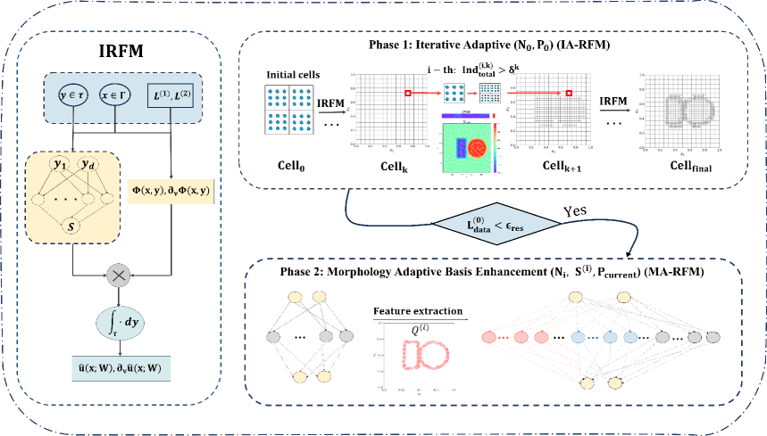
Figure 1: Integral Random Feature method (IRFM), Integral Adaptive Random Feature Method (IA-RFM), Morphology-Adaptive Random Feature Method (MA-RFM).

To save computational resources, a stopping criterion is added, which will terminate the iteration if $\mathcal{L}_{\text{data}}$ is less than a given threshold $\epsilon_{\text{res}}$. Finally, we obtain the following two-phase basis function augmented adaptive solver based on RFM. The baseline is the Integral Random Feature Method (IRFM), which uses a fixed set of training quadrature points. We refer to the first phase used in isolation as the Integral Adaptive Random Feature Method (IA-RFM). The complete two-phase algorithm is denoted as the Morphology-Adaptive Random Feature Method (MA-RFM). Figure 1 outlines the entire above procedure.

Algorithm 2 Morphology-Adaptive Random Feature Method (MA-RFM)

0: Computational domain $\Omega$, quadrature domain $V_{0}$, initial mesh $\text{Cell}_{0}$, initial network $\mathcal{N}_{0}$, initial number of basis functions $M_{0}$, $n^{d}$ Gauss points in the reference cell, weights $\gamma_{\text{grad}},\gamma_{\text{abs}}$, refinement threshold $\delta$, tolerance $\varepsilon$, max iterations max_iter, the number of measurement points $N_{s}$, set of basis function types $\mathcal{F}=\{\Phi_{\text{jump}},\Phi_{\text{Gauss}},\Phi_{\text{noise}},\cdots\}$, threshold $t_{\text{grad}}$, $t_{\text{abs}}\in(0,1)$, test points $P_{\text{test}}$, initial training points $\mathcal{P}_{0}$, max enhancement iteration $I_{\text{max}}$, residual tolerance $\varepsilon_{\text{res}}$.

0: Final network $\mathcal{N}_{\text{final}}$ and solution $S_{\text{final}}$.

1: Train $\mathcal{N}_{0}$ to obtain the coefficients $s^{(0)}$, initial hidden layer $H^{(0)}$, the final number of integral points $n_{\text{integral}}$, final integral points $\mathcal{P}_{\text{final}}$ and final $\text{Cell}_{\text{final}}$ by IA-RFM. Compute the value and its gradient field $\nabla S^{(0)}$ on $P_{\text{test}}$. Calculate the data loss $\mathcal{L}^{(0)}_{\text{data}}(s^{(0)},\mathcal{P}_{\text{final}})$.

2: if $\mathcal{L}_{\text{data}}^{(0)}<\varepsilon_{\text{res}}$ then

3:  $i=0$.

4: else

5:  for $i=1$ to $I_{\text{max}}$ do

6:   Identify regions: $\mathcal{Q}^{(i-1)}=\cup_{k}\mathcal{Q}_{k}^{(i-1)}=\mathcal{Q}_{\text{abs}}(S^{(i-1)})$ or $\mathcal{Q}_{\text{grad}}(S^{(i-1)})$ or $\mathcal{Q}_{\text{abs}}(S^{(i-1)})\cap$ $\mathcal{Q}_{\text{grad}}(S^{(i-1)})$.

7:   for each identified region $\mathcal{Q}_{k}^{(i-1)}\subset\mathcal{Q}^{(i-1)}$ do

8:    Select the basis type $\mathcal{T}_{k}\in\mathcal{F}$ based on the characteristics of $\mathcal{Q}_{k}^{(i-1)}$ and $S^{(i-1)}$.

9:    Estimate distribution of shape parameters $\mathcal{D}_{k}(\bm{\theta})$ for $\mathcal{T}_{k}$ based on $\mathcal{Q}_{k}^{(i-1)}$.

10:    Sample parameters $\bm{\theta}_{k}^{(i,j)}\sim\mathcal{D}_{k}(\bm{\theta})$ and add new basis functions:

$$\phi_{k}^{(i,j)}(\bm{x};K^{(i,j)},\bm{\theta}_{k}^{(i,j)})=\sigma_{\mathcal{T}_{k}}(\bm{x};K^{(i,j)},\bm{\theta}_{k}^{(i,j)}),\ k=1,\cdots,N,\ j=1,\cdots,M_{k}.$$

11:   end for

12:   Construct the enhanced network $\mathcal{N}_{i}$ by incorporating all new basis functions $\{\phi_{k}^{(i,j)}\}_{k=1,j=1}^{N,M_{k}}$:

$$H^{(i)}=H^{(i-1)}+\{\phi_{k}^{(i,j)}\}_{k=1,j=1}^{N,M_{k}},\quad\mathcal{N}_{i}(\bm{x})=f_{\text{out}}\circ H^{(i)}\circ H_{0}(\bm{x}).$$

13:   Retrain to obtain ${s}^{(i)}$ and ${S}^{(i)}$ through $\mathcal{N}_{i}$.

14:   Calculate the data loss $\mathcal{L}_{\text{data}}^{(i)}(s^{(i)},\mathcal{P}_{\text{final}})$.

15:   if $\mathcal{L}_{\text{data}}^{(i)}<\varepsilon_{\text{res}}$ then

16:    break

17:   end if

18:  end for

19: end if

20: $\mathcal{N}_{\text{final}}\leftarrow\mathcal{N}_{i}$, $S_{\text{final}}\leftarrow S^{(i)}$.

21: Return $\mathcal{N}_{\text{final}},S_{\text{final}}$.

3.3 Tikhonov regularization and stability analysis

In this section, we discuss the suitability and stability of this framework.

Denote Dirichlet, Neumann boundary data as $U_{D},U_{N}$, and the basis functions in $\Psi_{k_{1}}^{(1)}$, $\Psi_{k_{1}}^{(2)}$ is either after or before the MA-RFM.

$$U_{D}=\begin{bmatrix}U_{k_{1}}\\ \vdots\\ U_{k_{N}}\end{bmatrix},\quad U_{N}=\begin{bmatrix}\frac{\partial U_{k_{1}}}{\partial n}\ \\ \vdots\\ \frac{\partial U_{k_{N}}}{\partial n}\end{bmatrix},\quad\Psi_{D}=\begin{bmatrix}\Psi_{k_{1}}^{(1)}\\ \vdots\\ \Psi_{k_{N}}^{(1)}\end{bmatrix},\quad\Psi_{N}=\begin{bmatrix}\Psi_{k_{1}}^{(2)}\\ \vdots\\ \Psi_{k_{N}}^{(2)}\end{bmatrix}.$$

$$U=\begin{bmatrix}\text{Real}(U_{D})\\ \text{Imag}(U_{D})\\ \text{Real}(U_{N})\\ \text{Imag}(U_{N})\\ \end{bmatrix}\in\mathbb{R}^{n\times 1},\quad\Psi_{M}=\begin{bmatrix}\text{Real}(\Psi_{D})\\ \text{Imag}(\Psi_{D})\\ \text{Real}(\Psi_{N})\\ \text{Imag}(\Psi_{N})\\ \end{bmatrix}\in\mathbb{R}^{n\times M}.$$

For the discrete inverse problem stemming from our model, we have a linear system of the form:

$$\Psi_{\text{M}}\bm{s}=U.$$ (37)

Typically, such problems are ill-posed, as $\Psi_{\text{M}}$ has a large condition number, making the solution highly sensitive to noise in the data. Assume that the measured data $U^{\delta}$ relates to the true, noise-free data, $(U^{\delta})_{i}=(1+\delta\epsilon)\cdot(U_{\text{true}})_{i}$, $\epsilon\sim U(-1,1)$, $U^{\delta}=U_{\text{true}}+e$, where $e$ represents measurement noise. A direct inversion, as shown through SVD of $\Psi_{\text{M}}=U\Sigma V^{T}$, where $\Sigma=\text{diag}(\sigma_{1},\ldots,\sigma_{M})$, would yield a solution:

$$s^{\delta}=\sum_{i=1}^{M}\frac{\hat{u}_{i}^{*}U^{\delta}}{\sigma_{i}}\hat{v}_{i}=\sum_{i=1}^{M}\left(\frac{\hat{u}_{i}^{*}U_{\text{true}}}{\sigma_{i}}+\frac{\hat{u}_{i}^{*}e}{\sigma_{i}}\right)\hat{v}_{i}.$$ (38)

The term $\hat{u}_{i}^{*}e/\sigma_{i}$ demonstrates that small singular values $\sigma_{i}$ can drastically amplify the noise component, corrupting the solution. To counteract this effect, we employ Tikhonov regularization, which seeks to find a solution by minimizing a composite objective function:

$$\mathcal{L}_{\text{reg}}(\bm{s}^{\delta})=\|\Psi_{\text{M}}\bm{s}^{\delta}-U^{\delta}\|_{2}^{2}+\lambda_{\text{reg}}^{2}\|\bm{s}^{\delta}\|_{2}^{2}.$$

The regularization parameter $\lambda_{\text{reg}}>0$ balances the trade-off between fitting the data and controlling the norm of the solution. The solution becomes:

$$s^{\delta}=\sum_{i=1}^{M}f_{i}\left(\frac{\hat{u}_{i}^{*}U_{\text{true}}}{\sigma_{i}}+\frac{\hat{u}_{i}^{*}e}{\sigma_{i}}\right)\hat{v}_{i},\quad\text{where}\quad f_{i}=\frac{\sigma_{i}^{2}}{\sigma_{i}^{2}+\lambda_{\text{reg}}^{2}}.$$ (39)

The filter factors $f_{i}$ suppress the influence of noise associated with small singular values ($\sigma_{i}\ll\lambda_{\text{reg}}$), thus stabilizing the solution. The choice of $\lambda_{\text{reg}}$ is critical: a value too large introduces excessive bias, while a value too small fails to adequately suppress noise.

The following theorem provides the uniqueness and stability of the Tikhonov regularization solution.

Theorem 3.1 (Uniqueness and stability of Tikhonov regularization solution).

1. For any regularization parameter $\lambda_{\text{reg}}>0$, objective function $\mathcal{L}_{\text{reg}}(s^{\delta})=\|\Psi_{\text{M}}s^{\delta}-U^{\delta}\|_{2}^{2}+\lambda_{\text{reg}}^{2}\|s^{\delta}\|_{2}^{2}$, is strictly convex. Therefore, the minimization problem has a unique solution.

2. Let $S_{M}^{*}(\bm{x})=\sum s_{m}^{*}\phi_{m}(\bm{x})$ be the best approximation of the true source in the basis span $\{\phi_{m}(\bm{x})\}$, with coefficient vector $s^{*}$. Let $S_{M}^{\delta}$ be the regularized solution obtained from data $U^{\delta}$ with a coefficient vector $s^{\delta}=(\Psi_{\text{M}}^{T}\Psi_{\text{M}}+\lambda_{\text{reg}}^{2}I)^{-1}\Psi_{\text{M}}^{T}U^{\delta}$. Assume the noise level $\|U_{\text{true}}-U^{\delta}\|_{2}\leq\delta\|U_{\text{true}}\|_{2}\leq\delta_{\text{all}}$ and the model inconsistency is $\eta_{\text{M}}=\|\Psi_{\text{M}}s^{*}-U_{\text{true}}\|_{2}$. If the source condition $s^{*}=(\Psi_{\text{M}}^{T}\Psi_{\text{M}})^{\nu}w$ holds for some vector $w$, $0<\nu\leq 1$, then the error is bounded by:

   $$\|s^{\delta}-s^{*}\|_{2}\leq\frac{1}{2\lambda_{\text{reg}}}(\delta_{\text{all}}+\eta_{\text{M}})+C_{\nu}\lambda_{\text{reg}}^{2\nu}\|w\|_{2}.$$ (40)

   Furthermore, choosing the optimal parameter $\lambda_{\text{reg}}^{2}=\left(\frac{\delta_{\text{all}}+\eta_{\text{M}}}{4\nu C_{\nu}\|w\|_{2}}\right)^{\frac{2}{(2\nu+1)}}$ yields the minimum error bound:

   $$\|s^{\delta}-s^{*}\|_{2}\leq\left[(2\nu+1)\cdot(4\nu)^{-\frac{2\nu}{2\nu+1}}\cdot(C_{\nu}\|w\|_{2})^{\frac{1}{2\nu+1}}\right](\delta_{\text{all}}+\eta_{\text{M}})^{\frac{2\nu}{2\nu+1}}.$$ (41)

   where $C_{\nu}$ is positive bound constant, which only depends on $\nu$.

The proof of Theorem 3.1 is given in Appendix B.

Remark 2.

The item (a) demonstrates a key benefit of combining the IA-RFM or MA-RFM with Tikhonov regularization: it formulates the inverse problem as a strictly convex optimization, which guarantees the existence and uniqueness of the solution, providing a solid basis for the subsequent numerical algorithm. The item (b) guarantees an optimal $O((\delta_{\text{all}}+\eta_{\text{M}})^{\frac{2\nu}{2\nu+1}})$ convergence rate of coefficients and gives an a priori estimate of optimal $\lambda_{\text{reg}}$.

4 Numerical experiments

In this section, we present several 2-D and 3-D numerical examples, including continuous sources, discontinuous sources, and complex geometric sources, to evaluate the robustness and flexibility of the proposed algorithm.
Baseline Models. To show that we can better reconstruct the source with our framework, we set up baseline models. In addition to the IA-RFM, MA-RFM we derived before, we consider the IRFM which uses fixed training integral points in $V_{0}$, as well as the PINN which approximates $\{\{u^{k}_{\theta}\}_{k_{\text{min}}}^{k_{\text{ max}}},S_{\theta}\}$ based on the differential equation (10).
Date Generation. The artificial data can be generated by solving the forward problem (2).

$$u_{k}(\bm{x})=\int_{\tau}\Phi(k|\bm{x}-\bm{y}|)S(\bm{y})\,\mathrm{d}\bm{y},\quad\frac{\partial u_{k}}{\partial\nu}(\bm{x})=\int_{\tau}\frac{\partial\Phi(k|\bm{x}-\bm{y}|)}{\partial\nu(\bm{x})}S(\bm{y})\,\mathrm{d}\bm{y},\quad\bm{x}\in\Gamma,$$ (42)

Random noise is added to the artificial data in the magnitude and phase angle of the radiation field,

$$u^{\delta}_{k}:=u_{k}+\delta\epsilon_{1}|u_{k}|e^{i\pi\epsilon_{2}},\ \frac{\partial u^{\delta}_{k}}{\partial\nu}:=\frac{\partial u_{k}}{\partial\nu}+\delta\epsilon_{1}\bigl|\frac{\partial u_{k}}{\partial\nu}\bigr|e^{i\pi\epsilon_{2}},\ \epsilon_{1},\epsilon_{2}\sim U(-1,1),$$ (43)

where $\delta$ is the noise level. The observation data $\{u_{k},\frac{\partial u_{k}}{\partial\nu}\}$ are acquired on $\Gamma$ for $k\in[k_{\text{min}},k_{\text{max}}]$. In the following numerical examples, unless otherwise specified, we set $k_{\text{min}}=1$, $k_{i+1}=k_{i}+k_{\delta}$ for $i=1,\cdots,N-1$ with a uniform increment $k_{\delta}=4$. By default, observations are performed on a rectangular boundary. Let $\Omega=[a,b]\times[c,d]$, and the sample step size is $h_{x}=\frac{b-a}{N_{s}-1}$, $h_{y}=\frac{d-c}{N_{s}-1}$,

$$\mathcal{P}_{\text{mea}}=\bigcup_{i=0}^{N_{s}-1}\{(a,y)\cup(b,y)\mid y=c+ih_{y}\}\cup\{(x,c)\cup(x,d)\mid x=a+ih_{x}\},$$

$$\bigl\{u(k_{i},x_{s})\mid k_{i}\in\{k_{1},\ldots,k_{N}\},x_{s}\in\mathcal{P}_{\text{mea}}\bigr\},\quad\Bigl\{\frac{\partial u(k_{i},x_{s})}{\partial\nu}\mid k_{i}\in\{k_{1},\ldots,k_{N}\},x_{s}\in\mathcal{P}_{\text{mea}}\Bigr\}.$$

The unspecified $N_{s}$ refers to the number of observation points on one side of a rectangle or 1/4 of an arc. The relative $\|\cdot\|_{2}$ error of $S$ is given by:

$$E_{l^{2}}(S)=\frac{\sqrt{\frac{1}{n}\sum_{i=1}^{n}[S(\mathbf{x}_{i})-S_{\text{ex}}(\mathbf{x}_{i})]^{2}}}{\sqrt{\frac{1}{n}\sum_{i=1}^{n}S_{\text{ex}}^{2}(\mathbf{x}_{i})}}.$$ (44)

To select $\lambda_{\text{reg}}$, we adopt the posterior L-curve [40] method, which was initially proposed by Lawson and extended by Hansen, and the optimal regularization parameter corresponds to the corner of the curve.

Example 4.1. Prior parameters

In this example, we construct the source to validate Theorem 3.1.

Firstly, we create a random vector $w$, and directly compute $s^{*}=(\Psi_{\text{M}}^{T}\Psi_{\text{M}})^{\nu}w$, $S^{*}_{M}(\bm{x})=\sum s_{m}^{*}\phi_{m}(\bm{x})$ after generating a random feature space that defines the operator $\Psi_{\text{M}}$. Secondly, we generate $U_{\text{true}}$ with a precisely controlled model inconsistency $\eta_{\text{M}}$. The idea is based on the orthogonal decomposition of a vector space. $\forall\ U\in\mathbb{R}^{n}$ can be decomposed into the direct sum of the column space of the operator $\Psi_{\text{M}}$, denoted as $\text{col}(\Psi_{\text{M}})$, and its left null space $\text{ker}(\Psi_{\text{M}}^{T})$.

$$\mathbb{R}^{n}=\text{col}(\Psi_{\text{M}})\oplus\ker(\Psi_{\text{M}}^{T}).$$ (45)

Utilizing SVD, we have $\Psi_{\text{M}}=U\Sigma V^{T}$. If $\text{rank}(\Psi_{\text{M}})=r$, the first $r$ columns of $U\in\mathbb{R}^{n\times n}$ form the orthonormal basis for $\text{col}(\Psi_{\text{M}})$, while the last $n-r$ columns, denoted as $U_{\text{null}}$ form the orthonormal basis for $\text{ker}(\Psi_{\text{M}}^{T})$. $\bm{\eta_{\text{vec}}}$ is constructed as a random linear combination of the basis for the left null space: $\bm{\eta_{\text{vec}}}=U_{\text{null}}\cdot\bm{c}$, where $\mathbf{c}\in\mathbb{R}^{n-r}$ is a vector of random coefficients. To precisely control its norm to a target error value $\eta_{\text{M}}$ we normalize and scale it:

$$\bm{\eta}_{\text{vec}}\leftarrow\frac{\bm{\eta}_{\text{vec}}}{\|\bm{\eta}_{\text{vec}}\|_{2}}\times\eta_{\text{M}},$$ (46)

Finally, the synthetic data is generated by adding the explainable part $\Psi_{\text{M}}\cdot s^{*}$

$$U_{\text{true}}=\Psi_{\text{M}}\cdot\bm{s}^{*}+\bm{\eta}_{\text{vec}}.$$

Experimental setup: $V_{0}=[0,2]\times[0,2]$, $\Omega=[-0.5,2.5]\times[-0.5,2.5]$. Randomly generate vector $w$, $N_{s}=15$, $\nu=1$, $C_{\nu}=1$, $\eta_{\text{M}}=1e\text{-}4,1e\text{-}3,1e\text{-}2,1e\text{-}1,1$, $\delta=5\%$, $k_{\text{min}}=1,k_{\text{max}}=89$.
Hyperparameter settings: The activation function used for IRFM is $\sin$ , $R_{m}=20$, $M_{0}=3200$, initial integral mesh $N_{x}=N_{y}=1$ with $n_{x}=n_{y}=100$ Gauss points per cell.

The selection of the regularization parameter is guided by Theorem 3.1. Figure 2 illustrates that both the total error $\delta_{\text{all}}$ and regularization term $\lambda_{\text{reg}}^{2}$ increase with $\eta_{\text{M}}$. Meanwhile, the actual reconstruction error $\|s^{\delta}-s^{*}\|_{2}$ is approximately one order of magnitude below the theoretical upper bound. The close correspondence between the training and test set errors demonstrates the framework’s strong generalization capability. Figure 3 shows the reconstructed solution when $\eta_{\text{M}}=1$ with $E_{l^{2}}(S)=3.01\%$.

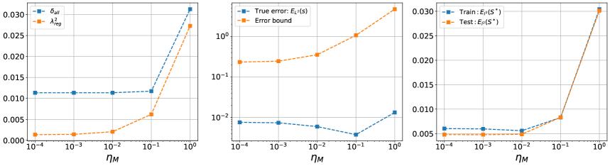
Figure 2: Example 4: Left) Prior parameters: $\eta_{\text{M}}$ versus $\delta_{\text{all}}$; Middle) $\lambda_{\text{reg}}^{2}$, $\|s^{\delta}-s^{*}\|_{2}$ and the theoretical error bounds; Right) $\|S^{\delta}-S^{*}_{M}\|_{2}$ for the training set versus the test set.

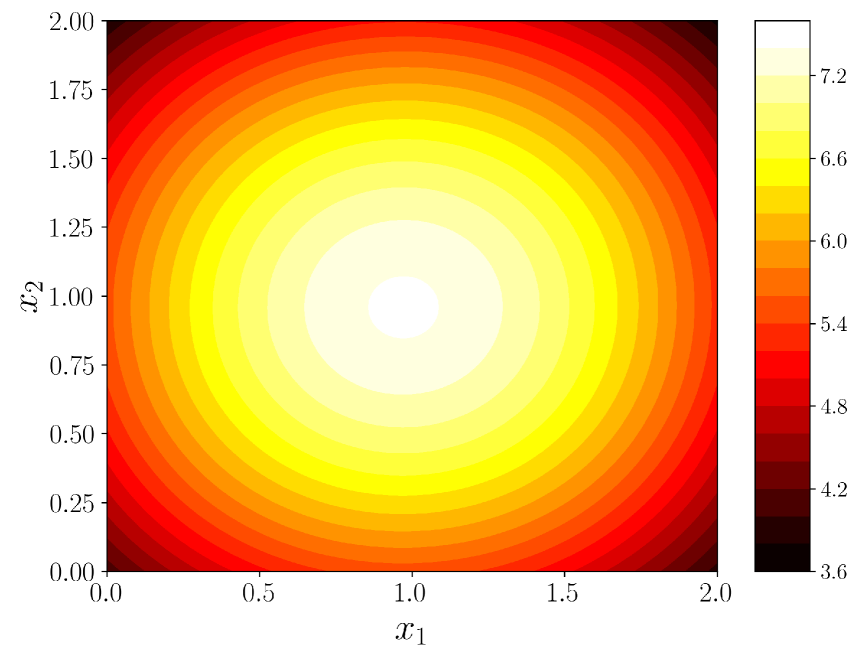
(a) $S_{M}^{*}(\bm{x})$

(b) $S^{\delta}(\bm{x})$

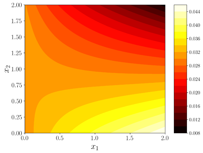
(c) Piece-wise relative error

Figure 3: Example 4: Prior parameters: IRFM results with $\eta_{\text{M}}=1$, $\nu=1$, $\delta=5\%$, $\delta_{\text{all}}=0.031$, $M_{0}=3200$, $N_{s}=15$, yield $3.01\%$ $E_{l^{2}}(S)$.

Example 4.2. Mountain shape source function

In the example, we aim to reconstruct a mountain-shaped source function

$$S(x_{1},x_{2})=1.1e^{-200((x_{1}-0.01)^{2})+(x_{2}-0.12)^{2}}-100(x_{2}^{2}-x_{1}^{2})e^{-90(x_{1}^{2}+x_{2}^{2})}.$$

We adopt the data generation procedure which generates Cauchy data on $\rho>R$ based on Dirichlet observations on $x=R$ based on an exterior extension from [17] to compare.

$$\nu^{\delta}(k,x)=\sum_{n\in\mathbb{Z}}\frac{H_{n}^{(1)}\left(k\rho\right)}{H_{n}^{(1)}\left(kR\right)}\hat{u}_{k,n}^{\delta}\mathrm{e}^{\mathrm{i}n\theta},\quad\partial_{\nu_{\rho}}\nu^{\delta}(k,x)=\sum_{n\in\mathbb{Z}}k\frac{H_{n}^{(1)^{\prime}}\left(k\rho\right)}{H_{n}^{(1)}\left(kR\right)}\hat{u}_{k,n}^{\delta}\mathrm{e}^{\mathrm{i}n\theta},\quad x\in\Gamma_{\rho},\ \rho>R.$$ (47)

$\hat{u}_{k,n}^{\delta}$ is the Fourier coefficient of the data $u^{\delta}(k,R,\theta)$. All other parameters, such as wavenumbers $K_{N}\cup\{k^{*}\}$ and the truncation number $N=2[\delta^{-1/3}]$, where [X] denotes the largest integer that is smaller than X + 1, are chosen to be identical to those in [17] (Thm 3.3, Rem 3.1). Here we use $N_{R}$, $N_{\rho}$ to denote the total number of observations on $\Gamma_{R}$, and the total number of data points generated on $\Gamma_{\rho}$, respectively.

Experimental setup: $V_{0}=[-0.3,0.3]\times[-0.3,0.3]$, $\Omega=B_{0.5}(0,0)$, $\rho=0.6$. The observation region is the circular arc $\Gamma_{R}=\partial\Omega$, and the generated region is $\Gamma_{\rho}$, noise level $\delta=5\%$, truncation number $N=6$.
Hyperparameter settings: The activation function used for IRFM and IA-RFM is $\sin$, $R_{m}=20$, $M_{0}=3200$, $N_{\text{generate}}=400$, initial integral mesh $N_{x}=N_{y}=5$ with $n_{x}=n_{y}=5$ Gauss points per cell. The maximum number of integral iteration max_iter=10, $\epsilon_{\text{res}}=0.5\delta$.

In order to understand the reason for the failure of PINN, we analyze its prediction for the inverse source problem with a loss function similar to (3.1). To simplify the Loss and reduce the difficulty caused by the penalty term, set the observation position and the artificial boundary to be $\Gamma_{\rho}$, and then use the paradigm triangulation inequality to get $\mathcal{L}_{\text{PINN}}$ as follows:

$$\mathcal{L}_{\text{PINN}} =\sum_{k=k_{1}}^{k_{N}}\Bigg(\lambda_{\text{pde}}\sum_{\bm{x}_{i}\in V_{0}}\left\|-(\Delta+k^{2})u_{NN}^{k}(\bm{x}_{i})-S_{NN}(\bm{x}_{i})\right\|_{l^{2}}^{2}+\lambda_{\text{bound}}\sum_{\bm{x}_{j}\in\Gamma_{\rho}}\left\|u^{k}_{NN}(\bm{x}_{j})-u^{k}(\bm{x}_{j})\right\|_{l^{2}}^{2}$$ (48)

$$+\lambda_{\text{radiation}}\sum_{\bm{x}_{j}\in\Gamma_{\rho}}\left\|\mathcal{T}^{k}(u^{k}_{NN}(\bm{x}_{j}))-\partial_{\nu}u^{k}(\bm{x}_{j})\right\|_{l^{2}}^{2}\Bigg).$$

The structures of $u_{NN}$ and $S_{NN}$ are [2, 50, 50, 2] and [2, 50, 50, 1], respectively. Set $n_{\text{pde}}=100^{2}$, $\lambda_{I}=1$, $\lambda_{\text{radiation}}=10$, $\lambda_{\text{bound}}=10$, and we perform noise-free experiments, with the other parameters consistent with the settings above. Training is first performed using 30,000 ADAM iterations, then the subsequent training is performed using 5,000 L-BFGS iterations. From results shown in Figure (4), we observe that PINN fails to reconstruct the source. Since in this framework, not only do we need $N+1$ networks to approximate the scattered fields $u$ and $S$, which is a very large number of parameters and difficult to balance with a multitude of penalties, but also $u$ is more oscillatory as $k$ gets larger, yet neural networks have difficulty in approximating high frequency.

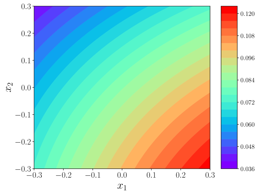
(a)

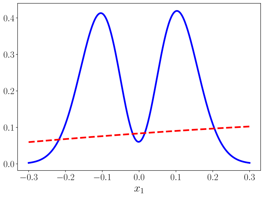
(b)

Figure 4: Example 4: Mountain shape source function: (a). PINN solution with $u_{NN}$: [2, 50, 50, 2] and $S_{NN}$: [2, 50, 50, 1] yields 99.68% $E_{l^{2}}(S)$. (b). The true solution ( ) and PINN solution (   ) at($x_{1}$,0).

According to Table 1, IA-RFM shows an overwhelming advantage in computational efficiency compared with the conventional Fourier method (FM) and IRFM. The number of generated points $N_{\rho}$ and integration points $n_{\text{integral}}$ are reduced by one and two orders of magnitude, respectively. Through its adaptive integration, it saves approximately 80% of the integration computations compared with IRFM, while simultaneously achieving a comparable or even superior $l^{2}$ error. This result strongly demonstrates that IA-RFM is able to intelligently and precisely allocate computational resources to the critical regions, thus achieving a balance between computational cost and solution accuracy. Subsequently, with noise level $\delta=10\%$ and $N_{\rho}$=100, and all other parameters remaining the same, the $E_{l^{2}}(S)$ is 1.38% with IA-RFM, which is shown in Figure 5.

In addition, it is worth mentioning that this experiment satisfies the convergence condition ($\epsilon_{\text{res}}<\delta$) in the first stage of the algorithm, and does not enable the basis function enhancement in the second stage, which suggests that IA-RFM is sufficient for solving this problem.

Table 1: Comparison of FM, IRFM, and IA-RFM with $N=6$, $\delta=5\%$ for mountain shape source.

Method	$N_{R}$	$N_{\rho}$	$n_{\text{integral}}$	$E_{l^{2}}(S)$
FM	50	5000	$800^{2}$	1.620%
	100	5000	$800^{2}$	1.150%
	200	5000	$800^{2}$	0.824%
	400	5000	$800^{2}$	0.629%
IRFM	50	400	$100^{2}$	0.735%
	100	400	$100^{2}$	0.638%
	200	400	$100^{2}$	0.580%
	400	400	$100^{2}$	0.560%
IA-RFM	50	400	2125	0.727%
	100	400	1975	0.651%
	200	400	1875	0.575%
	400	400	2025	0.557%

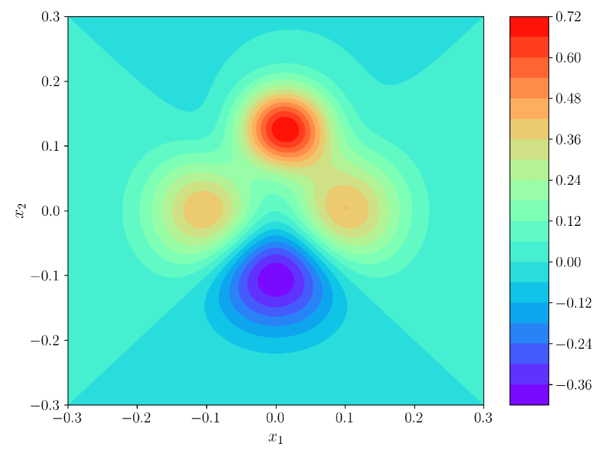
(a) True source

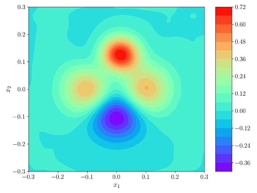
(b) Reconstructed source

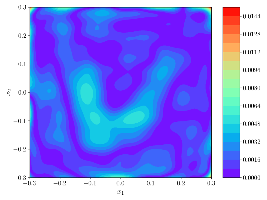
(c) Piece-wise absolute error

Figure 5: Example 4: Mountain shape source function: IA-RFM results with $\delta=10\%$, $M_{0}=3200$, $N_{s}=50$, $N_{\text{generate}}$=100, $\lambda_{\text{reg}}^{2}=7.84e\text{-}2$ yield 1.39% $E_{l^{2}}(S)$.

Example 4.3. Discontinuous source

In the following numerical experiments, a more challenging scenario is considered where the support of the source $\tau$, is a proper subset of $V_{0}$, $\tau\subsetneqq V_{0}$, which means the source is discontinuous within the region $V_{0}$.

$$S(x_{1},x_{2})=\mathcal{X}_{B_{r}},\quad B_{r}(0.5,0.5)=\{(x_{1},x_{2})|(x_{1}-0.5)^{2}+(x_{2}-0.5)^{2}\leq r^{2},r=0.2\}.$$

Experimental setup: $V_{0}=[0,1]\times[0,1]$, $\Omega=[-0.5,1.5]\times[-0.5,1.5]$. $k_{\text{min}}$=1, $k_{\text{max}}=89$, $N_{s}$=15.

Hyperparameter settings: The activation function Tanh is used for IRFM and IA-RFM. Tanh, sigmoid are used for MA-RFM. $R_{m}=20$, $M_{1}=M_{0}$, $M_{\text{total}}=M_{0}+M_{1}$,

$$\phi_{1}^{(j)}(\bm{x};K_{1}^{(j)},\bm{\theta}_{1}^{(j)}) =\text{sigmoid}\left(K_{1}^{(j)}\cdot\left((r_{1}^{(j)})^{2}-\|\bm{x}-\bm{c}_{1}^{(j)}\|_{2}^{2}\right)\right)\ ,\ j=1,2,\cdots,M_{1}.$$

The initial integral mesh $N_{x_{1}}=N_{x_{2}}=4$ with $n_{x_{1}}=n_{x_{2}}=3$, max_iter=10. $K_{1}^{(j)}\sim U(1000,20000)$, the tolerance $\epsilon_{c}=3\sim 5\%$ and $\epsilon_{r}=10\%$ are applied to the center coordinates of the detected circle and radius, respectively.

Table 2 compares the performance of MA-RFM with IRFM. The results indicate that the accuracy of IRFM quickly saturates as the number of basis functions $M$, increases. In contrast, MA-RFM not only improves the reconstruction accuracy by approximately 37% but also demonstrates superior computational efficiency by requiring fewer integration points. To further validate robustness, we conducted a noise-resistance experiment with parameters set as follows: $M_{0}=1600$, $M_{1}=1600$, $\epsilon_{c}=3\%$, $\epsilon_{r}=5\%-10\%$. As shown in Table 3, the results for MA-RFM under noise levels $\delta$ reveal that even with a high noise level of $\delta=10\%$, the relative error is only 13.17%—a slight increase compared to the noiseless baseline. This provides strong evidence of the superior stability and noise-resistance capabilities of MA-RFM.

Table 2: Comparison of IRFM and MA-RFM for discontinuous source.

Method	$M_{\text{total}}$	$n_{\text{integral}}$	$\lambda^{2}_{\text{reg}}$	$l^{2}$-error
IRFM	800	$100^{2}$	1.00e-4	22.78%
	1600	$100^{2}$	1.00e-4	20.12%
	3200	$100^{2}$	1.00e-18	17.99%
	6400	$100^{2}$	1.00e-26	16.80%
MA-RFM	800	$6624$	1.00e-8	14.35%
	1600	$6462$	1.00e-12	12.22%
	3200	$6138$	1.00e-20	11.12%
	6400	$5382$	1.00e-24	10.50%

Table 3: The shape parameters and reconstruction errors for the discontinuous source.

$\delta$	0	0.5%	1%	5%	10%	20%
$\hat{c}$	[0.497, 0.498]	[0.495, 0.498]	[0.497, 0.495]	[0.5, 0.498]	[0.5, 0.497]	[0.497, 0.498]
$\hat{r}$	0.2193	0.2176	0.2209	0.2209	0.2209	0.2176
$\lambda^{2}$	1.00e-28	1.00e-6	1.00e-6	1.00e-4	1.00e-3	1.00e-2
$l^{2}\mbox{-}S$	10.80%	12.38%	12.63%	12.89%	13.17%	13.84%

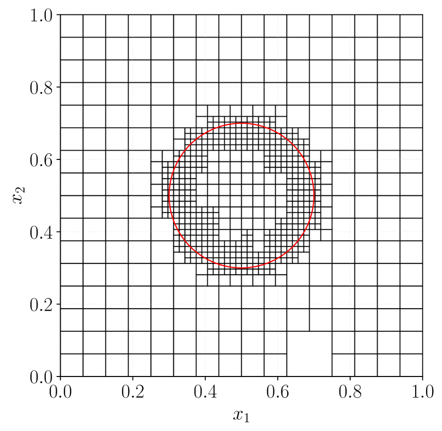
(a) $\text{Cell}_{\text{final}}$

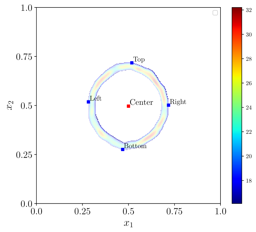
(b) $\mathcal{Q}_{\text{grad}}$

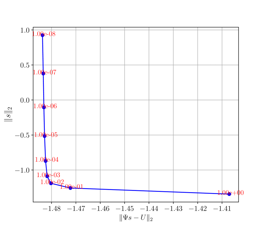
(c) L-curve

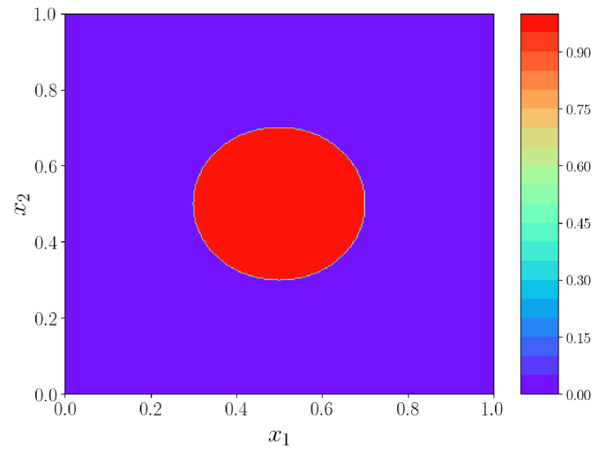
(d) True source

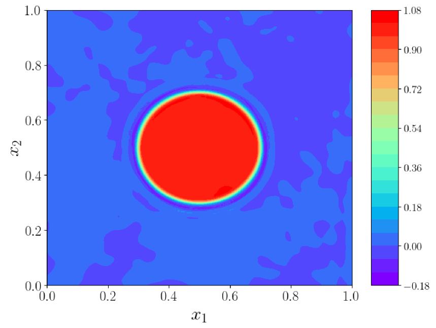
(e) Reconstructed source

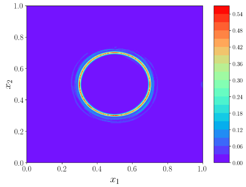
(f) Piece-wise absolute error

Figure 6: Example 4: Discontinuous source: MA-RFM results with $\delta=10\%$, $M_{\text{total}}=3200$, $N_{s}=15$, $\lambda_{\text{reg}}^{2}=1e\text{-}4$ yield 13.17% $E_{l^{2}}(S)$. (a) shows the $\text{Cell}_{\text{final}}$ with IA-RFM, and the red line represents the true interface. (b) displays the $\mathcal{Q}_{\text{grad}}$ with $t_{\text{grad}}=1/2$. $\hat{c}=[\frac{x_{1,\text{left}}+x_{1,\text{right}}}{2},\frac{x_{2,\text{bottom}}+x_{2,\text{top}}}{2}]$. $\hat{r}=\max\{\frac{x_{1,\text{right}}-x_{1,\text{left}}}{2},\frac{x_{2,\text{top}}-x_{2,\text{bottom}}}{2}\}$, $\epsilon_{c}=3\%$, $\epsilon_{r}=5\%\text{-}10\%$. (c) records the L-curve $\text{log}_{10}(\|\Psi\cdot\bm{s}-U\|_{2})$-$\text{log}_{10}(\|\bm{s}\|_{2})$ with different $\lambda_{\text{reg}}^{2}$.

Example 4.4. Two circle sources

Consider the reconstruction of the discontinuous source function defined in the rectangular domain $V_{0}$.

$$S(x_{1},x_{2})=\left\{\begin{array}[]{ccc}0.5\exp(-550r_{1}^{2}),&\quad\mathrm{in}\ B_{r}(\hat{x}_{0},0),\\ 0.5\exp(-550r_{2}^{2}),&\quad\mathrm{in}\ B_{r}(\bar{x}_{0},0),\\ 0,\quad\text{elsewhere.}\end{array}\right.$$

$r_{1}=\sqrt{(x_{1}-\hat{x}_{0})^{2}+x_{2}^{2}},\ r_{2}=\sqrt{(x_{1}-\bar{x_{0}})^{2}+x_{2}^{2}}$ and $B_{r}(x_{0},0)$=$\{\bm{x}:(x_{1}-x_{0})^{2}+x_{2}^{2}\leq r^{2}\}$.

Experimental setup: $V_{0}=[-0.30,0.30]\times[-0.30,0.30]$, $\Omega=[-0.35,0.35]\times[-0.35,0.35]$, $\hat{x}_{0}=-0.06$, $\bar{x}_{0}=0.08$, $r=0.06$, $N_{s}=20$, $k_{\text{min}}=1$, $k_{\text{max}}=77$.

Hyperparameter settings: The initial activation function for MA-RFM is Tanh with $R_{m}=2$, added by two families of truncated Gaussian basis.

$$\phi_{k}^{(j)}(\bm{x};K^{(j)}_{k},\bm{\theta}_{k}^{(j)}) =\text{sigmoid}\left(K^{(j)}_{k}\cdot\left((r^{(j)}_{k})^{2}-\|\bm{x}-\bm{c}_{k}^{(j)}\|_{2}^{2}\right)\right)\cdot\text{exp}\left(-v^{(j)}_{k}\cdot\|\bm{x}-\bm{c}_{k}^{(j)}\|_{2}^{2}\right)$$

$$k=1,2,\ j=1,2,\cdots,M_{k}.$$

The exponential component shapes the morphology of the source, with the parameter $v$ controlling its decay rate. $K_{k}^{(j)}\sim U(1000,20000)$, $v_{k}^{(j)}\sim U(0,1000)$. $M_{0}=2400$, $M_{1}=2000$, $M_{2}=2000$, initial integral mesh $N_{x_{1}}=N_{x_{2}}=4$ with $n_{x_{1}}=n_{x_{2}}=3$, max_iter=10. $\epsilon_{c}=5\%$, $\epsilon_{r}=5\%$.

Figure 7 illustrates the mesh evolution and detected morphology points of IA-RFM. The mesh becomes denser in regions where a jump occurs and where the absolute values of the solution are relatively large. And the MA-RFM results in Figure 8, show the 6.15% $E_{l^{2}}(S)$ with $\delta=10\%$.

Table 4: The shape parameters and reconstruction errors for two circle sources.

$\delta$	$n_{\text{integral}}$	$\hat{c}_{1}$	$\hat{c}_{2}$	$\hat{r}_{1}$	$\hat{r}_{2}$	$\lambda_{\text{reg}}^{2}$	$E_{l^{2}}(S)$
0%	5220	[-6.28e-2, -9.97e-4]	[8.07e-2, -9.97e-4]	0.06379	0.06379	1.00e-34	3.98%
0.5%	1710	[-6.18e-2, -9.97e-4]	[8.07e-2, -9.97e-4]	0.06379	0.06379	1.00e-5	6.21%
1%	1953	[-6.18e-2, -9.97e-4]	[8.07e-2, -9.97e-4]	0.06379	0.06379	1.00e-5	5.60%
5%	1980	[-6.38e-2, -9.97e-4]	[8.07e-2, -1.39e-17]	0.06379	0.06478	1.00e-5	6.34%
10%	2034	[-6.38e-2, -9.97e-4]	[8.07e-2, -9.97e-4]	0.06379	0.06478	1.00e-4	6.15%
20%	2088	[-6.28e-2, -9.97e-4]	[8.07e-2, -9.97e-4]	0.06379	0.06379	1.00e-4	7.53%

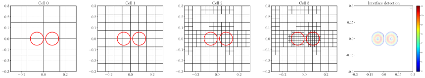
Figure 7: Example 4: Two circle sources: grid division diagram for IA-RFM with $\delta=10\%$, $M_{0}=2400$, Tanh, $R_{m}=2$. The last one shows the $\mathcal{Q}_{\text{grad}}$ with $t_{\text{grad}}$=1/2.8.

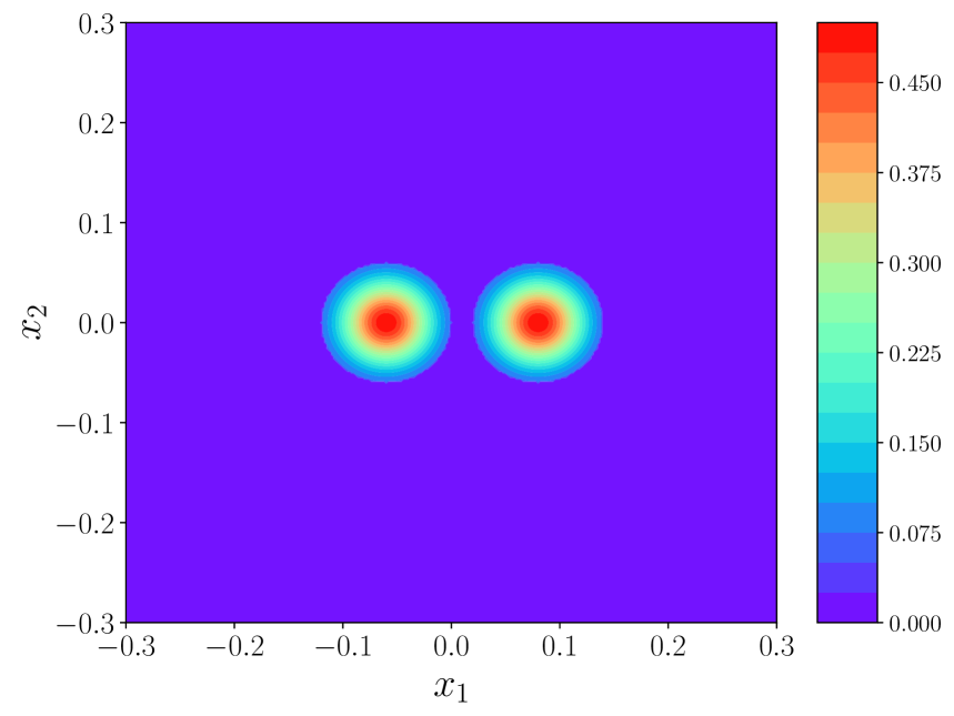
(a) True source

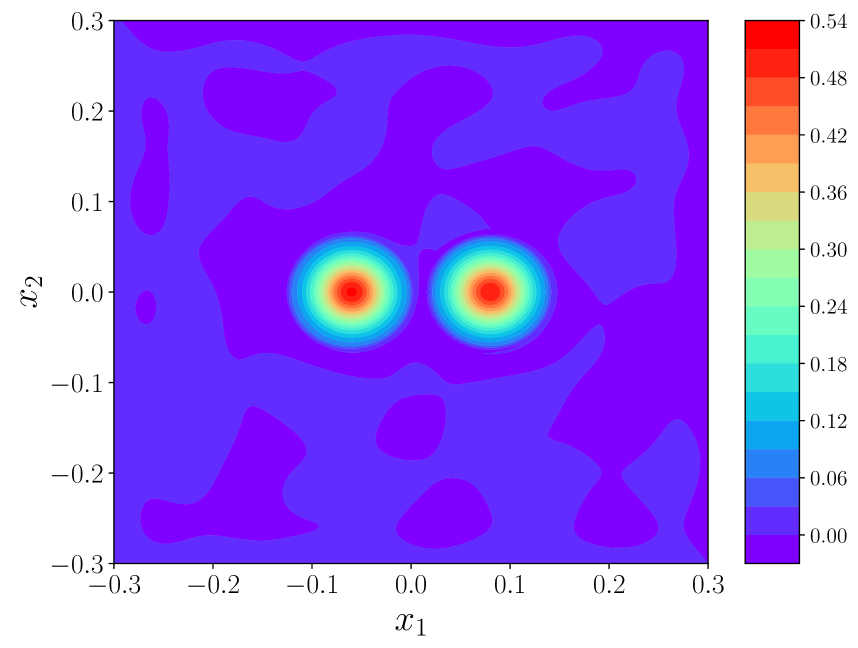
(b) Reconstructed source

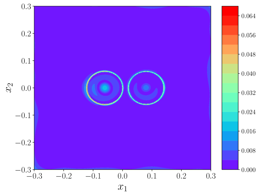
(c) Piece-wise absolute error

Figure 8: Example 4: Two circle sources: MA-RFM results with $\delta=10\%$, $M_{\text{total}}=6400$, $N_{s}=20$ and $\lambda_{\text{reg}}^{2}=1e\text{-}4$ yield an 6.15% $E_{l^{2}}(S)$.

Example 4.5. One rectangle and one circle

The spatial proximity of two sources poses a significant challenge for the inverse source problem. This difficulty arises because the fine, high-frequency details of the small gap between them are smoothed away during wave propagation. Consequently, the signals generated by the sources on the observation boundary become highly coupled and difficult to distinguish. In what follows, we consider a numerical example with closely spaced sources to demonstrate the resolution capability of MA-RFM.

$$S(x_{1},x_{2})=\mathcal{X}_{B}-\mathcal{X}_{C},$$

$B=\{(x_{1},x_{2})|\ (x_{1}-0.5)^{2}+(x_{2}-0.5)^{2}\leq r^{2},r=0.2\}$, $C=\{(x_{1},x_{2})|\ 0.29\leq x_{1}\leq 0.49,0.3\leq x_{2}\leq 0.7\}$.
Experimental setup: $V_{0}=[0,1]\times[0,1]$, $\Omega=[-0.5,1.5]\times[-0.5,1.5]$. $k_{\text{min}}$=1, $k_{\text{max}}=89$, $N_{s}$=10, $\delta=5\%$.
Hyperparameters settings: The activation function for IRFM and IA-RFM is Tanh with $R_{m}=20$, and for MA-RFM, the basis functions are Tanh and sigmoid, corresponding to circular and rectangular shape functions, respectively.

$$\phi_{1}^{(j)}(\bm{x};K_{1}^{(j)},\bm{\theta}_{1}^{(j)}) =\text{sigmoid}\left(K_{1}^{(j)}\cdot\left((r^{(j)}_{1})^{2}-\|\bm{x}-\bm{c}_{1}^{(j)}\|^{2}_{2}\right)\right),\ j=1,2,\cdots,M_{1}.$$

$$\phi_{2}^{(j)}(\bm{x};K_{2}^{(j)},\bm{\theta}_{2}^{(j)}) =\text{sigmoid}\Bigl(-K^{(j)}_{2}\cdot\max\{x_{1}-c_{1}^{(j)}-\frac{\text{width}^{(j)}}{2},x_{2}-c_{2}^{(j)}-\frac{\text{height}^{(j)}}{2}\}\Bigr),$$

$$\hskip 250.00038ptj=1,2,\cdots,M_{2}.$$

$c_{1}^{(j)},c_{2}^{(j)}$ are the width and height corresponding to the center of the circle and the width and height of the rectangle, respectively. $M_{1}=M_{2}=0.5M_{0}$. $\epsilon_{c}=5\%$, $\epsilon_{r}=5\%$ for the center and radius of the detected circle, respectively. $\epsilon_{\text{width}}=20\%$, $\epsilon_{\text{height}}=15\%$ for the width and height of the detected rectangle, respectively. The initial mesh is $N_{x_{1}}=N_{x_{2}}=4$ with $n_{x_{1}}=n_{x_{2}}=3$, $R_{m}=20$, max_iter=10.

The results in Table 5 clearly demonstrate the superiority of MA-RFM. It accomplishes this with up to 25% with fewer $n_{\text{integral}}$ but 40% higher accuracy. A noise experiment is conducted to test the stability and robustness of MA-RFM. Set $M_{0}=1600$ and $M_{1}=M_{2}=2400$, while the remaining parameters are kept consistent with the previous. The mesh evolution is illustrated in Figure 9. Figure 10 illustrates the $\mathcal{Q}^{(i)}$, $i=1,\ 2$ and reconstruction of MA-RFM with two iterations. Table 6 shows that even under 10% noise level, the relative error can still be maintained at 15.84%. The results discussed before demonstrate that MA-RFM can capture the small gap between two nearby sources very well and remain robust.

Table 5: Compare of IRFM and MA-RFM with $\delta=5\%$ for one rectangle and one circle.

Method	$M_{\text{total}}$	$n_{\text{integral}}$	$\lambda^{2}$	$E_{l^{2}}(S)$
IRFM	800	$100^{2}$	1.00e-4	25.79%
	1600	$100^{2}$	1.00e-5	22.44%
	3200	$100^{2}$	1.00e-6	21.15%
	6400	$100^{2}$	1.00e-6	20.25%
MA-RFM	800	$8001$	1.00e-4	16.13%
	1600	$7569$	1.00e-5	14.80%
	3200	$7569$	1.00e-5	15.19%
	6400	$7542$	1.00e-4	15.63%

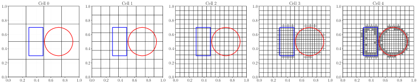
Figure 9: Example 4: One rectangle and one circle: grid division diagram for IA-RFM with $\delta=5\%$, $M_{0}=2400$, Tanh, $R_{m}=2$.

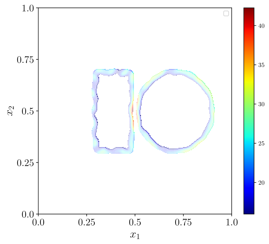
(a) $\mathcal{Q}^{(0)}=\mathcal{Q}^{(0)}_{\text{abs}}\cap\mathcal{Q}^{(0)}_{\text{grad}}$

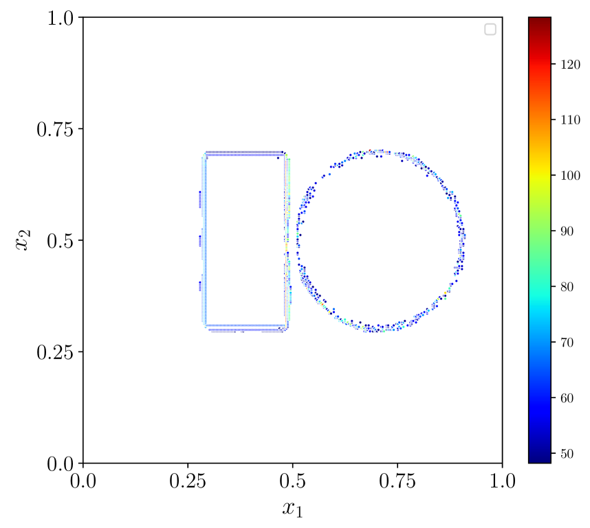
(b) $\mathcal{Q}^{(1)}=\mathcal{Q}^{(1)}_{\text{abs}}\cap\mathcal{Q}^{(1)}_{\text{grad}}$

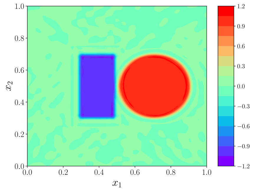
(c) Reconstructed source

Figure 10: Example 4: One rectangle and one circle: (a), (b) show the gradient of points from $\mathcal{Q}^{(i)}=\mathcal{Q}^{(i)}_{\text{abs}}\cap\mathcal{Q}^{(i)}_{\text{grad}}$ chosen from ${S}^{(i)}$, $\nabla{S}^{(i)}$, $i=0,1$, with $t_{\text{abs}}=1/3.2$, $t_{\text{grad}}=1/2.8$. (c) shows the reconstruction results with $\delta=5\%$, $M_{0}=1600$, $M_{1}=M_{2}=2400$, $N_{s}=10$ and $\lambda_{\text{reg}}^{2}=1e\text{-}4$ yielding 15.78% $E_{l^{2}}(S)$ using MA-RFM.

Table 6: The shape parameters and reconstruction errors for one rectangle and one circle.

$\delta$	0	0.5%	1%	5%	10%	20%
$\hat{c}_{\text{rec}}$	[0.389, 0.498]	[0.387, 0.5]	[0.382, 0.497]	[0.388, 0.498]	[0.390, 0.493]	[0.387, 0.490]
$\hat{c}_{\text{circle}}$	[0.708, 0.498]	[0.714, 0.497]	[0.711, 0.498]	[0.709, 0.497]	[0.709, 0.495]	[0.711, 0.497]
$\hat{\text{width}}$	0.2193	0.2226	0.2326	0.2193	0.2226	0.2293
$\hat{\text{height}}$	0.4252	0.4286	0.4419	0.4385	0.4286	0.4618
$\hat{r}$	0.2027	0.2126	0.2109	0.2110	0.2043	0.2110
$\lambda^{2}$	1.00e-24	1.00e-6	1.00e-5	1.00e-4	1.00e-4	1.00e-3
$E_{l^{2}}(S)$	13.77%	15.30%	15.02%	15.78%	15.84%	16.34%

Example 4.6. Complex geometry

Now consider complex geometries to test the generality of MA-RFM. Consider the kidney-shaped line with the contour implicit function expression

$$((x-x_{0})^{2}+(y-y_{0})^{2}-4a^{2})^{3}=108a^{4}(y-y_{0})^{2}.$$ (49)

Use the level set function $\psi(x,y)$ to represent regions,

$$\psi(x,y)=((x-x_{0})^{2}+(y-y_{0})^{2}-4a^{2})^{3}-108a^{4}(y-y_{0})^{2},$$

$\tau=\{(x,y)|\ \psi(x,y)\leq 0\}$, introduce the radial parameter $r$, parameterize the region to calculate the measurement data.

$$\left\{\begin{aligned} &x(s,\varphi)=r(3a\cos\varphi-a\cos 3\varphi),\\ &y(s,\varphi)=r(3a\sin\varphi-a\sin 3\varphi),\ r\in[0,1],\ \phi\in[0,2\pi].\end{aligned}\right.$$ (50)

Consider a composite source that combines a continuous source and a discontinuous source.

$$S(x_{1},x_{2}) =S_{\text{kidney}}(x_{1},x_{2})+S_{\text{gauss}}(x_{1},x_{2}),$$

$$S_{\text{kidney}}(x_{1},x_{2}) =\mathcal{X}_{\{(x_{1},x_{2}):\ \psi(x_{1},x_{2})\leq 0\}},$$

$$S_{\text{gauss}}(x_{1},x_{2}) =1.2\exp(-125((x_{1}-0.3)^{2}+(y-0.6)^{2})).$$

Experimental setup: $V_{0}=[0,1]\times[0,1]$, $\Omega=[-0.5,1.5]\times[-0.5,1.5]$, $x_{0}=0.6$, $y_{0}=0.25$, $a=0.05$. $k_{\text{min}}$=1, $k_{\text{max}}=101$, $N_{s}$=20, $\delta=5\%$.
Hyperparameter settings The activation function for IA-RFM is Tanh, $R_{m}=20$, $\epsilon_{\text{res}}=0.5\delta$. The basis function used in MA-RFM is sigmoid, comprising a general form and a supplementary circle basis function to compensate for the undesirable position of the detected boundary at the interface jump obtained using the continuous basis function Tanh.

$$\phi_{1}^{(j)}(\bm{x};K_{1}^{(j)},\theta^{(j)}_{1}) =\text{sigmoid}\left(K_{1}^{(j)}\cdot d_{1}^{(j)}(\bm{x};\rho^{(j)})\right),\ \ j=1,\cdots,M_{1}.$$

$$\phi_{2}^{(j)}(\bm{x};K_{2}^{(j)},\bm{\theta}_{2}^{(j)}) =\text{sigmoid}\left(K_{2}^{(j)}\cdot\left((r_{2}^{(j)})^{2}-\|\bm{x}-\bm{c}_{2}^{(j)}\|_{2}^{2}\right)\right),\ j=1,\cdots,M_{2}.$$

Denote the detected boundary as $\mathcal{P}^{(0)}=\{\bm{x}:\psi(\bm{x})=0\}$. $\mathcal{P}^{(0)}$ are firstly smoothed using B-splines, resulting in $\widehat{\mathcal{P}}^{(0)}$, which is then scaled along its normal direction:

$$\bm{x}^{(j)}=\bm{x}+\rho^{(j)}\bm{n}\cdot\bm{x},\ \forall\bm{x}\in\widehat{\mathcal{P}}^{(0)}.$$

This process forms a family of contour points $\hat{\mathcal{P}}^{(j)}=\{\bm{x}:\psi^{(j)}(\bm{x};\rho^{(j)})=0\}$. The SDF is defined as:

$$d_{1}^{(j)}(\bm{x};\rho^{(j)})=\left\{\begin{aligned} &1,\quad&\psi_{1}^{(j)}(\bm{x};\rho^{(j)})\leq 0,\\ &-1,\quad&\psi_{1}^{(j)}(\bm{x};\rho^{(j)})>0,\end{aligned}\right.$$

$\rho^{(j)}\sim U(-0.03,-0.01)$, $K_{1}^{(j)},K^{(j)}_{2}\sim U(1000,30000)$, $r_{2}^{(j)}\sim U(0,0.05)$, $t_{\text{grad}}$=1/3, $M_{1}=M_{0}=1600$, $M_{2}=\#\widehat{\mathcal{P}}^{(0)}=1740$, $\bm{c}_{2}^{(j)}\in\widehat{\mathcal{P}}^{(J)}$. The initial mesh $N_{x_{1}}=N_{x_{2}}=4$ with $n_{x_{1}}=n_{x_{2}}=3$, max_iter=10.

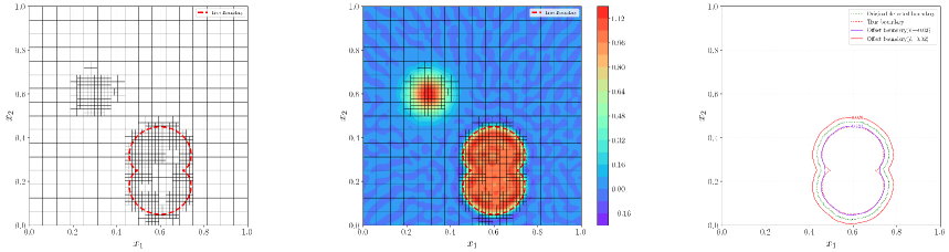
Figure 11: Example 4: Complex geometry: Adaptive meshing $\text{Cell}_{\text{final}}$ with $E_{l^{2}}(S)=19.53\%$ and numerical approximation of the kidney boundary. The red and green dashed lines are the true boundary, the numerically detected boundary obtained from $\mathcal{Q}_{\text{grad}}$, respectively. The red and green solid lines correspond to the numerical level sets for $\rho=0.02,-0.02$, which serve as the numerical scaling boundary.

Figure 11 illustrates the $\text{Cell}_{\text{final}}$ using IA-RFM and numerical scaled interface and real interface. Figure 12(c) shows the reconstruction using MA-RFM with $\delta=5\%$.

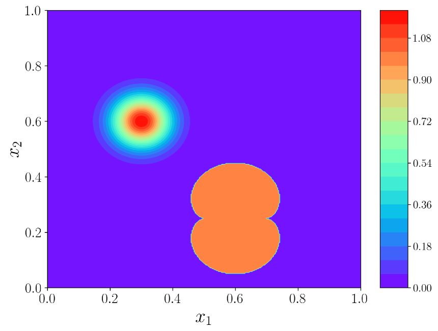
(a) True source

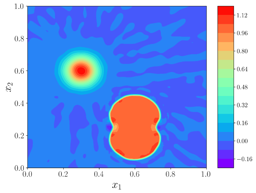
(b) Reconstructed source

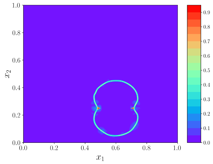
(c) Piece-wise absolute error

Figure 12: Example 4: Complex geometry: MA-RFM results with $\delta=5\%$, $M_{0}=1600$, $M_{1}=1600$, $M_{2}=1740$, $\lambda_{\text{reg}}^{2}=1e\text{-2}$ yield 13.05% $E_{l^{2}}(S)$.

Example 4.7. Three-dimensional $C^{0}$ source

Consider $S(\bm{x})=S^{\bm{a}}(\bm{x})-S^{\bm{b}}(\bm{x})$

$$S^{\bm{y}}(\bm{x})=\begin{cases}0.2-r_{\bm{y}},&\mathrm{if}\quad r_{\bm{y}}<0.2,\\ \quad 0,&\mathrm{if}\quad r_{\bm{y}}\geqslant 0.2,\end{cases}$$

where $r_{\bm{y}}=\sqrt{(x_{1}-y_{1})^{2}+(x_{2}-y_{2})^{2}+(x_{3}-y_{3})^{2}}$, $\bm{a}=(0.3,0.5,0.3)$, $\bm{b}=(0.5,0.5,0.8)$.

Experimental setup: $V_{0}=[0,1]^{3}$, $\Omega=[-0.5,1.5]^{3}$, $k_{\text{min}}$=1, $k_{\text{max}}=81$, $N_{s}$=10, $\delta=5\%$.

Hyperparameter settings: $V_{0}=[0,1]^{3}$, $\Omega=[-0.5,1.5]^{3}$, $k_{\text{min}}$=1, $k_{\text{max}}=81$, $N_{s}$=10, $\delta=5\%$. The activation function for IA-RFM is Tanh, $R_{m}=10$, $\epsilon_{\text{res}}=0.05\delta$. The basis functions in MA-RFM are of a conical type, using ReLU and Gaussian functions as follows:

$$\phi_{k,\text{ReLU}}^{(j)}(\bm{x};\bm{\theta}_{k}^{(j)}) =\text{ReLU}\left(r_{k}^{(j)}-\|\bm{x}-\bm{c}_{k}^{(j)}\|_{2}\right),\ k=1,2,\ j=1,2,\cdots,M_{k,\text{ReLU}},$$

$$\phi_{k,\text{exp}}^{(j)}(\bm{x};\bm{\theta}_{k}^{(j)}) =\exp\left(-v_{k}^{(j)}\cdot\|\bm{x}-\bm{c}_{k}^{(j)}\|_{2}^{2}\right),\ k=1,2,\ j=1,2,\cdots,M_{k,\text{exp}}.$$

where $v^{(j)}_{k}$ determines the decay rate of the exponential term and is selected by the Full Width at Half Maximum (FWHM) method. We first define a 1-D slice of the initial solution $S_{\text{num}}^{(0)}$ along the $i$-th dimension as $g_{i}(t):=S_{\text{num}}^{(0)}(...,t,...)$, $t\in[0,1]$. FWHM is then determined by

$$t_{\text{max}}:=\mathop{\arg\max}_{t}|g_{i}(t)|,\quad I_{\text{half}}=\frac{1}{2}g_{i}(t_{\text{max}}),$$

$$\text{FWHM}_{i}:=\sup\{t\mid g_{i}(t)\geq I_{\text{{half}}}\}-\inf\{t\mid g_{i}(t)\geq I_{\text{half}}\},$$

$$v_{\text{min}}=\frac{2.355^{2}}{2\cdot\max\limits_{i}\text{FWHM}_{i}},\ v_{\text{max}}=\frac{2.355^{2}}{2\cdot\min\limits_{i}\text{FWHM}_{i}},$$

$v^{(j)}_{k}\sim U(0.5v_{\text{min}},2v_{\text{max}})$. $c^{(j)}_{k}$ are selected based on the peak locations of $S_{\text{num}}^{(0)}$, as illustrated in Figure 13. $M_{0}=3600$, $M_{k,\text{ReLU}}=M_{k,\text{exp}}=900$, $v^{(j)}_{k}\sim U(5.775,25.2)$. $r_{k}^{(j)}\sim U(0.18,0.26)$, $\hat{c}_{k}^{(j)}\sim U(\hat{c}_{k}-0.02,\hat{c}_{k}+0.02)$, $k=1,2$. The initial mesh $N_{x_{1}}=N_{x_{2}}=4$ with $n_{x_{1}}=n_{x_{2}}=3$, max_iter=10.

See Figure 13 for the detection details. And Figure 14 shows the reconstruction using MA-RFM.

(a)

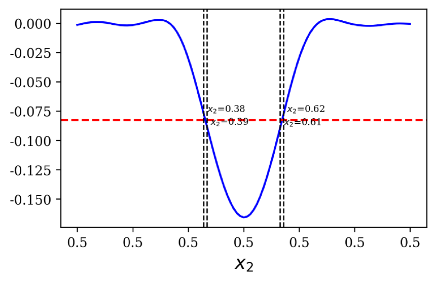
(b)

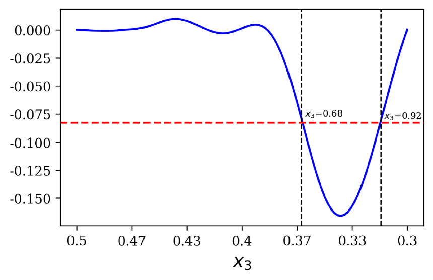
(c)

(d)

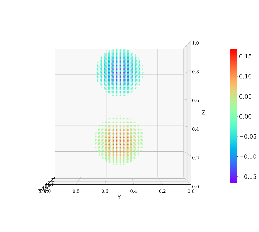
(e)

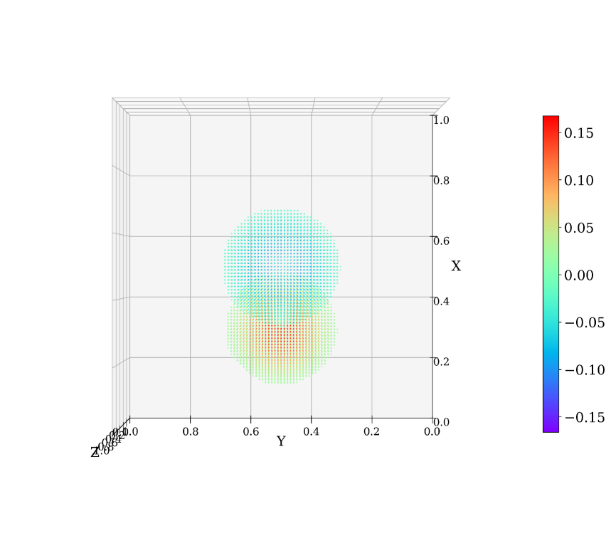
(f)

Figure 13: Example 4: Three-dimensional $C^{0}$ source: (a),(b),(c) show the numerical solution $g_{i}(x)$ for the slice $S_{\text{num}}^{(0)}$ (blue solid line). The red line denotes the value $I_{\text{half}}$, and the black line shows the position of the independent variable corresponding to $\frac{1}{2}I_{\text{half}}$. (d),(e),(f) show the $S_{\text{num}}^{(0)}$ of points from $\mathcal{Q}_{\text{grad}}$ from different perspectives. Based on $\mathcal{Q}_{\text{grad}}$ one can determine that $\hat{c}_{1}=(0.3,0.5,0.3)$, $\hat{c}_{2}=(0.5,0.5,0.8)$. $\hat{c}_{k}^{(j)}\sim U(\hat{c}_{k}-0.02,\hat{c}_{k}+0.02)$, $k=1,2$.

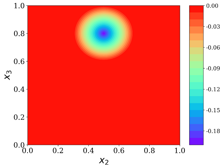
(a) True source at $(0.3,x_{2},x_{3})$

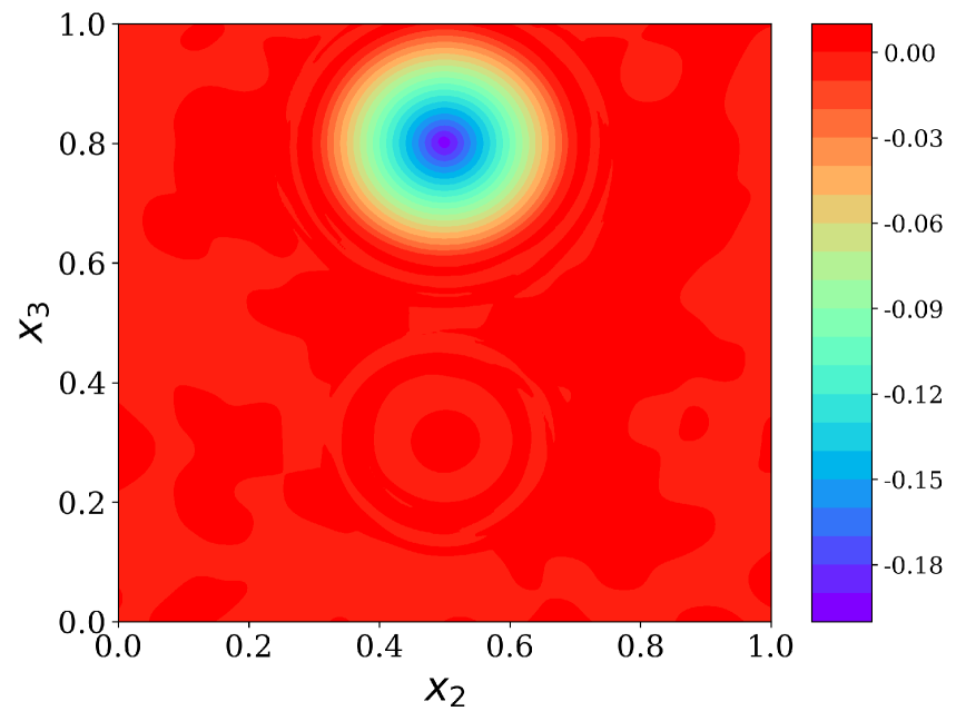
(b) Reconstruction at $(0.3,x_{2},x_{3})$

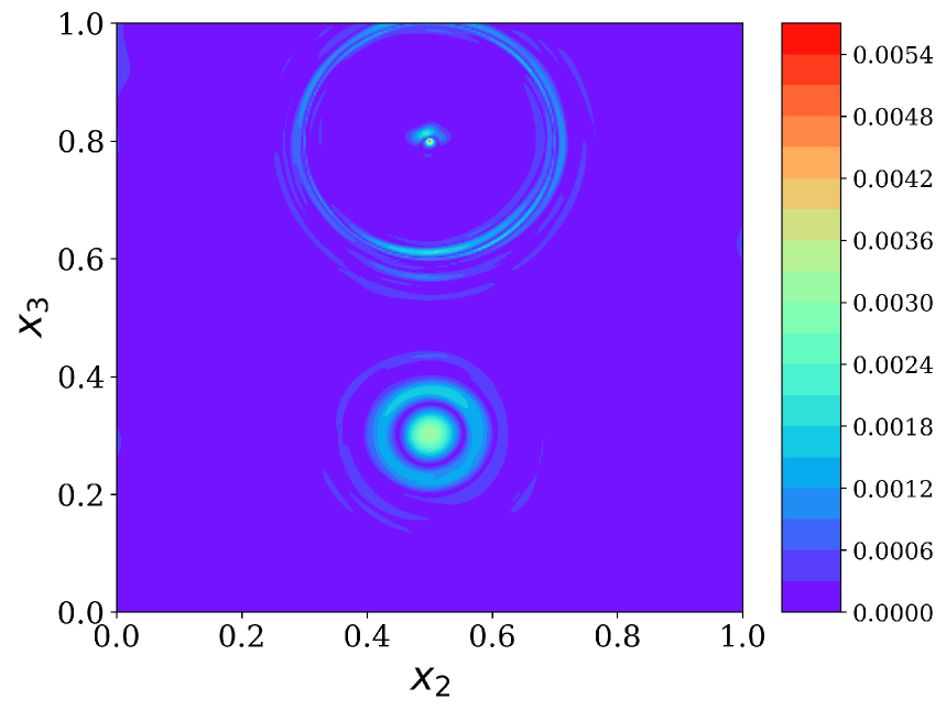
(c) Piece-wise absolute error

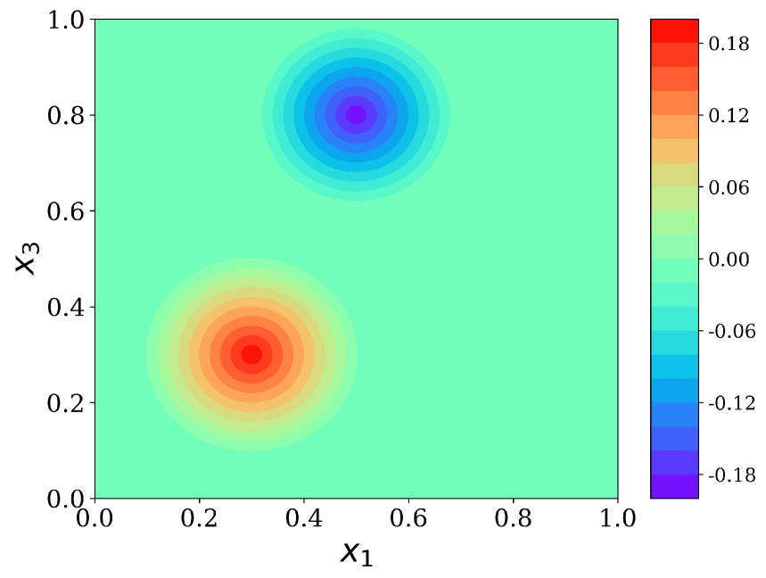
(d) True source at $(x_{1},0.5,x_{3})$

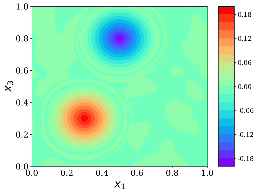
(e) Reconstruction at $(x_{1},0.5,x_{3})$

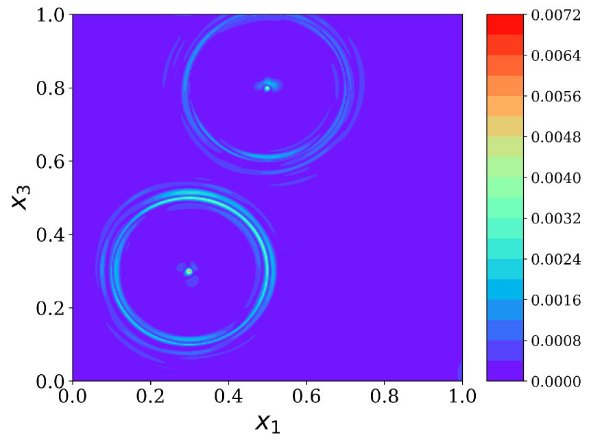
(f) Piece-wise absolute error

Figure 14: Example 4: Three-dimensional $C^{0}$ source: MA-RFM results with $\delta=5\%$, $M_{0}=3600$, $M_{k,\text{ReLU}}=M_{k,\text{exp}}=900$, $\lambda_{\text{reg}}^{2}=1e\text{-}4$ yield 1.35% $E_{l^{2}}(S)$.

Example 4.8. Three-dimensional donut

Next, consider a 3-D “donut” segment source, which can be parameterized as follows:

$$\left\{\begin{aligned} &x_{1}(u,v,w)=(R_{1}+wR_{2}\cos v)\cos u,\\ &x_{2}(u,v,w)=(R_{1}+wR_{2}\cos v)\sin v,\\ &x_{3}(u,v,w)=wR_{2}\sin v,\end{aligned}\right.$$ (51)

$0\leq u\leq 2\pi$, $0\leq v\leq 2\pi$, $0\leq w\leq 1$. $R_{1}=0.25$, $R_{2}=0.15$.

The source function is defined as 1 inside the donut and 0 outside.

Experimental setup: $V_{0}=[-0.5,0.5]\times[-0.5,0.5]$,   $\Omega=[-0.75,0.75]\times[-0.75,0.75]$. $k_{\text{min}}$=1, $k_{\text{max}}=81$, $N_{s}$=10, $\delta=5\%$. Dirichlet data only.

Hyperparameter settings: The activation function for IA-RFM is Tanh, $R_{m}=20$. The basis function used in MA-RFM is sigmoid.

$$d^{(j)}_{1}(\bm{x};\bm{\theta}_{1}^{(j)})=-\psi^{(j)}_{1}(\bm{x};\bm{\theta}_{1}^{(j)})=(r_{1}^{(j)})^{2}-\left(\left(\sqrt{(x_{1}-c_{1})^{2}+(x_{2}-c_{2})^{2}}-R^{(j)}_{1}\right)^{2}+(x_{3}-c_{3})^{2}\right),$$

$$\phi_{1}^{(j)}(\bm{x};K_{1}^{(j)},\bm{\theta}_{1}^{(j)})=\text{sigmoid}\left(K_{1}^{(j)}\cdot d^{(j)}_{1}(\bm{x};\bm{\theta}_{1}^{(j)})\right),\ j=1,\cdots,M_{1}.$$

$M_{0}$=3600, $M_{1}=1600$. $r_{1}^{(j)}\sim U(0.14,0.16)$, $R_{1}^{(j)}\sim U(0.24,0.26)$, $\bm{c}_{1}^{(j)}\sim U(-0.015,0.015)$, $K_{1}^{(j)}\sim U(2000,50000)$. The initial mesh $N_{x_{1}}=N_{x_{2}}=4$ with $n_{x_{1}}=n_{x_{2}}=3$, max_iter=10.

Details of detected results with IA-RFM and final reconstruction are shown in Figure 15. The IA-RFM results show that points with high gradients and absolute values form a toroidal donut-like structure, which prompts our choice of the similarly shaped level set function, $\psi^{(j)}_{1}$ for an adaptive approximation.

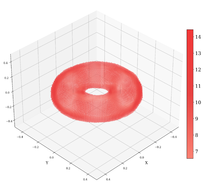
(a)

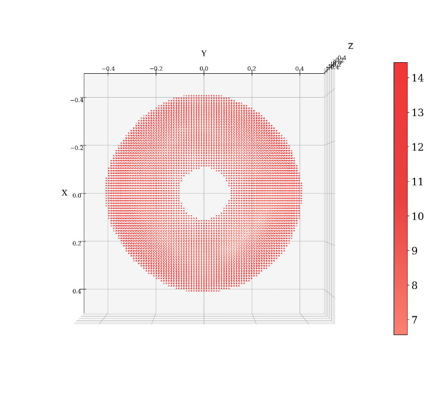
(b)

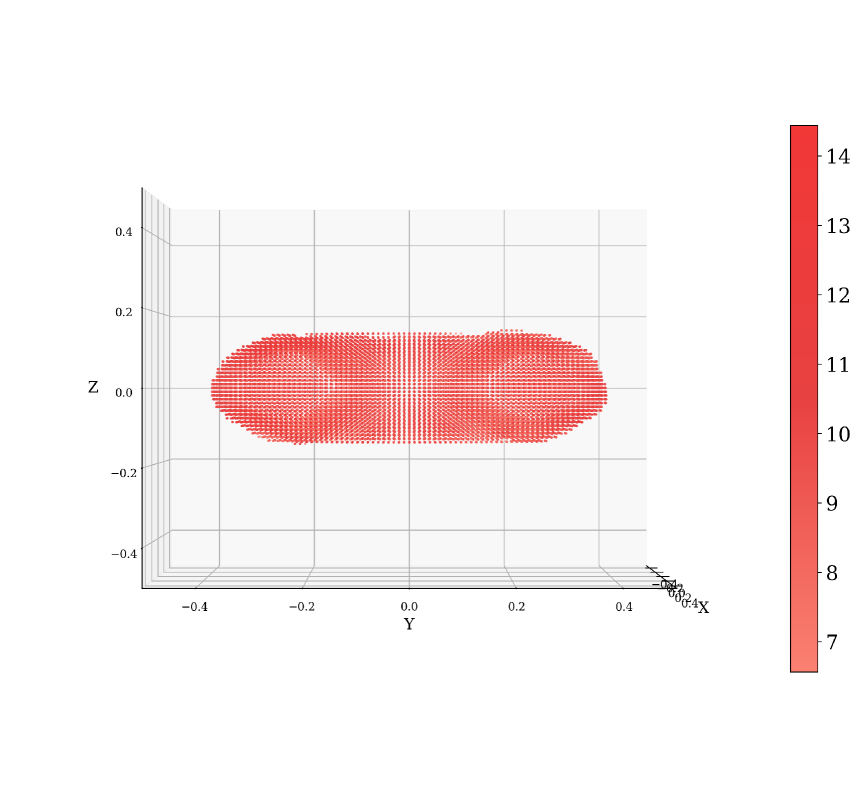
(c)

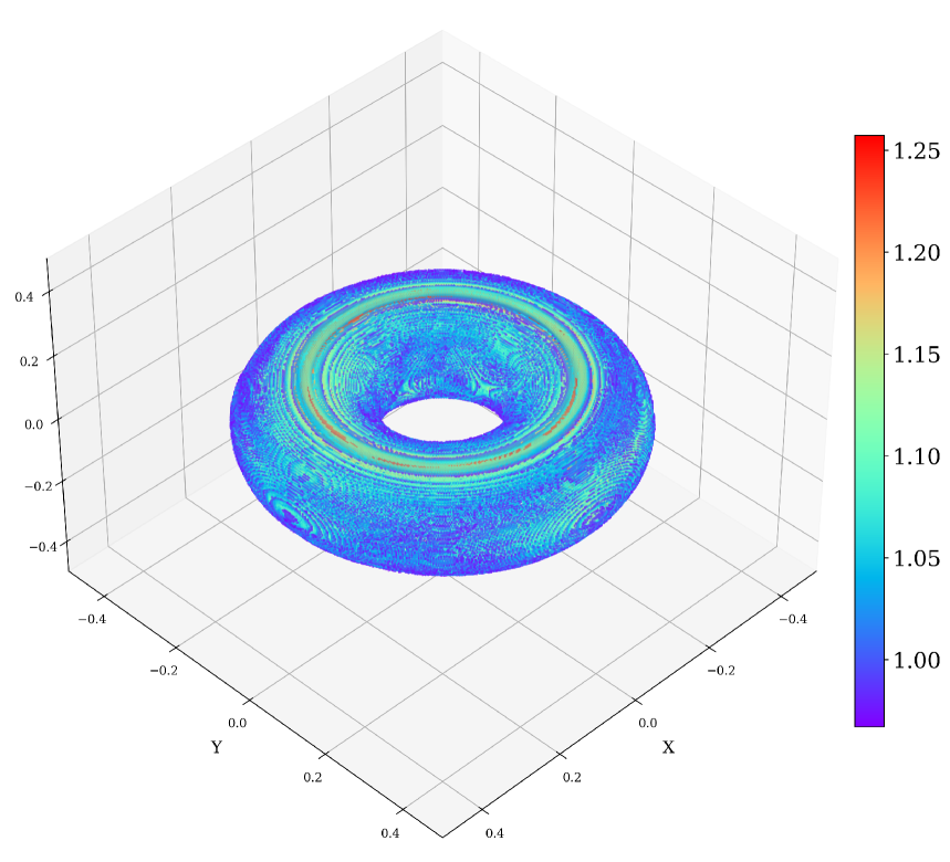
(d)

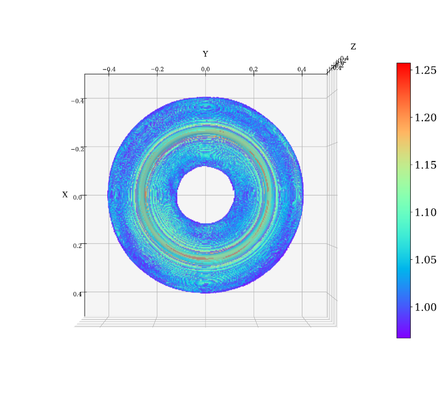
(e)

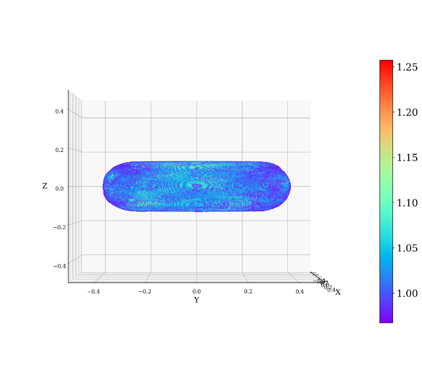
(f)

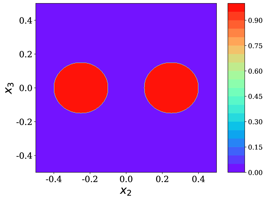
(g) True source at $(0,x_{2},x_{3})$

(h) True source at $(x_{1},0,x_{3})$

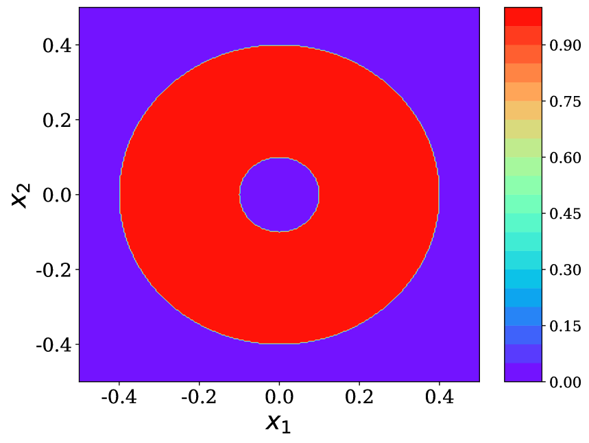
(i) True source at $(x_{1},x_{2},0)$

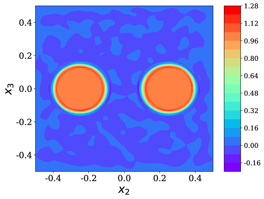
(j) Reconstruction at $(0,x_{2},x_{3})$

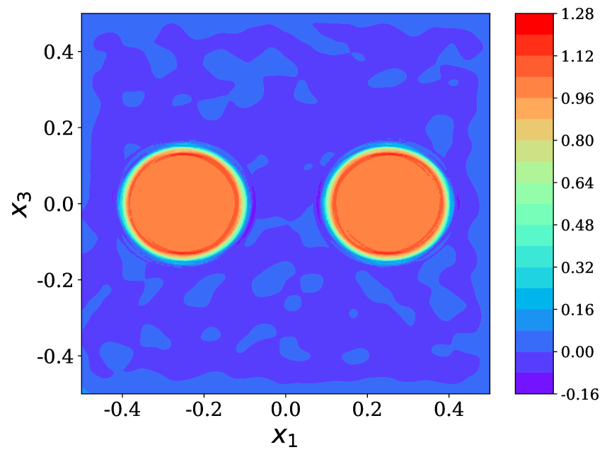
(k) Reconstruction at $(x_{1},0,x_{3})$

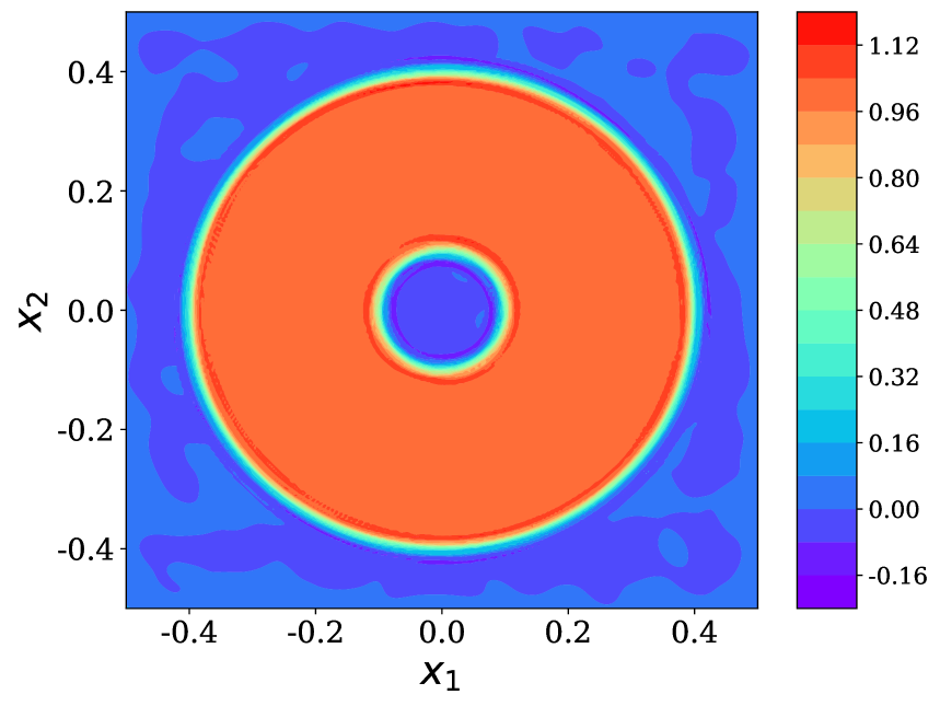
(l) Reconstruction at $(x_{1},x_{2},0)$

Figure 15: Example 4: Three-dimensional donut: (a),(b),(c) show the gradient of points from $\mathcal{Q}$ with $t_{\text{abs}}=1/2.2$, $t_{\text{grad}}=1/2.2$, from which we get 6 key points: [-0.39,-0.08,-0.01], [-0.39,-0.08,-0.01], [-0.06,-0.39,-0.03], [-0.04,0.39,-0.03], [-0.12,-0.22,-0.15], [-0.18,0.16,0.15] to determine the shape parameters. (d),(e),(f) show the reconstruction using MA-RFM from different perspectives, and (j),(k),(l) show the 2-D cross section results with $M_{0}=3600$, $M_{1}=1600$, $\delta=5\%$ and $\lambda_{\text{reg}}^{2}=10^{-7}$, yielding $E_{l^{2}}(S)=15.50\%$.

Example 4.9. Limited aperture

In practical applications, only partial data may be available. To simulate this condition, we directly test the IA-RFM in a scenario where only partial measurement data is acquired. We consider the problem of reconstructing a source function consisting of four Gaussian peaks:

$$S(x_{1},x_{2}) =\mathrm{e}^{-300\left(\left(x_{1}-0.15\right)^{2}+\left(x_{2}-0.15\right)^{2}\right)}+\mathrm{e}^{-300\left(\left(x_{1}+0.15\right)^{2}+\left(x_{2}-0.15\right)^{2}\right)}$$

$$+\mathrm{e}^{-300\left(\left(x_{1}+0.15\right)^{2}+\left(x_{2}+0.15\right)^{2}\right)}+\mathrm{e}^{-300\left(\left(x_{1}-0.15\right)^{2}+\left(x_{2}+0.15\right)^{2}\right)}.$$

Experimental setup: $V_{0}=[-0.3,0.3]\times[-0.3,0.3]$,   $\Omega=B_{0.55}(0,0)$, $\Gamma=\partial\Omega$, $k_{\text{min}}$=1, $k_{\text{max}}=101$, $\delta=1\%$. The number of measurement points on each quarter-arc of the boundary is $N_{s}=25$.
Hyperparameter settings: The activation function for IA-RFM is $\sin$, $R_{m}=20$, $M_{0}=3200$. The initial mesh $N_{x_{1}}=N_{x_{2}}=4$ with $n_{x_{1}}=n_{x_{2}}=3$, max_iter=10.

Table 7 and Figure 16 show the $E_{l^{2}}(S)$ for different apertures with noise level $\delta=1\%$. It can be observed that when $\theta_{\text{max}}=\pi$, the error is already very small. For $\theta_{\text{max}}=\pi/2$, we can still roughly determine the locations of the sources. This result indicates that the proposed algorithm exhibits good performance and effectiveness under limited aperture conditions.

Table 7: $E_{l^{2}}(S)$ with aperture $[0,\theta_{\text{max}}]$ and $\delta=1\%$, $M=3200$ using IA-RFM for limited aperture.

$\theta_{\text{max}}$	2$\pi$	$3\pi/2$	$\pi$	$\pi/2$
$l^{2}\mbox{-}S$	0.27%	0.32%	0.59%	22.79%

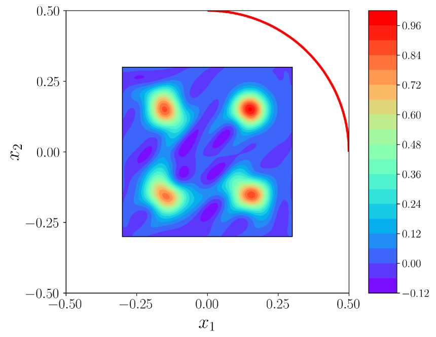
(a)

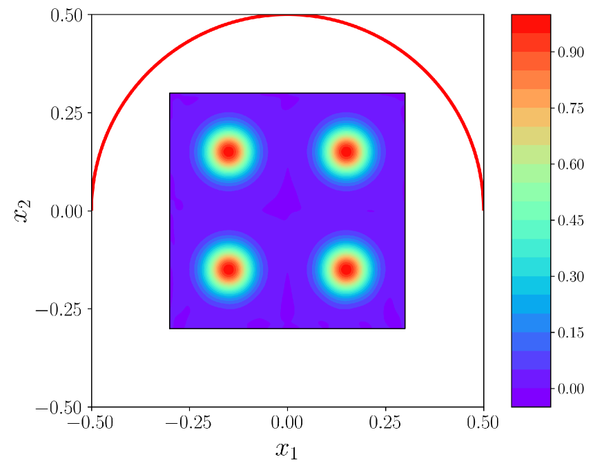
(b)

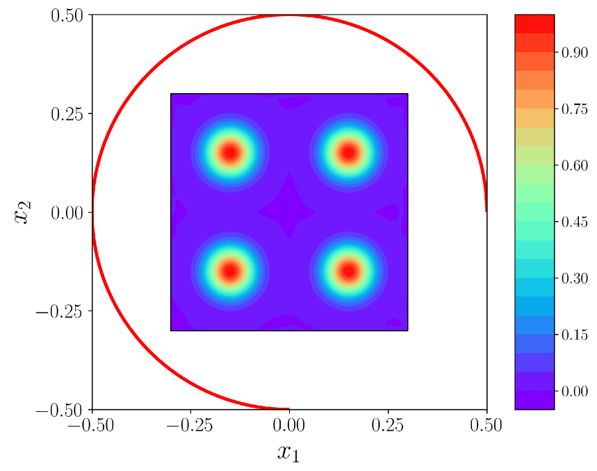
(c)

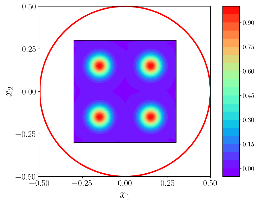
(d)

Figure 16: Example 4 : Limited aperture: effect of the measurement aperture $\theta_{\text{max}}$ on the source reconstruction. The contour plots show the results for (a) $\theta_{\text{max}}=\pi/2$, (b) $\theta_{\text{max}}=\pi$, (c) $\theta_{\text{max}}=3\pi/4$, and (d) $\theta_{\text{max}}=2\pi$ with $\delta=1\%$. The measurement locations are indicated by the red outer arc.

5 Conclusion

In conclusion, we have proposed a novel, efficient framework –MA-RFM– that successfully tackles the long-standing challenge of complex source geometries in the Helmholtz inverse source problem. The core of our method is a synergistic combination of spectral methods and neural networks. Specifically, we employ an integral equation formulation to satisfy the radiation condition as a hard constraint. Concurrently, we propose the MA-RFM, which uses the posterior information to design targeted basis functions of neural networks, enabling precise capture of local singular features of the source. Extensive numerical experiments conducted on a series of sources with complex situations validate the superior performance of our framework. The results show that the proposed method not only achieves high accuracy in all test cases but also reduces the computational cost by two to three orders of magnitude compared to traditional methods while maintaining the same level of precision. Furthermore, we believe that the underlying concept of morphology-based adaptive basis function enhancement holds significant promise for broader applications in other complex scientific and engineering computing problems.

Appendix A. Proof of Theorem 2.1

Proof.

Assume $S=S_{1}-S_{2}$ and $u=u_{1}-u_{2}$. The source of $u$ is $S$, and its support is contained in $\tau_{1}\cup\tau_{2}$. In situation (a), (b), (c), $u$ is a radiating solution to the homogeneous Helmholtz equation in the exterior domain $\mathbb{R}^{d}\backslash\overline{\Omega}$, which implies $u(k_{j},\bm{x})=0$ for all $\bm{x}\in\mathbb{R}^{d}\backslash\overline{\Omega}$ from Theorem 9.10 in [37]. And for (d), we can deduce $u(k_{j},\bm{x})=0$ from Holmgren’s uniqueness theorem [41]. All of the situations imply that

$$u(k_{j},\bm{x})=0\quad and\quad\partial_{\nu}u(k_{j},\bm{x})=0,\quad\forall\bm{x}\in\Gamma.$$ (52)

Now, let $w_{k_{j}}$ be any solution to the homogeneous Helmholtz equation $\Delta w_{k_{j}}+k_{j}^{2}w_{k_{j}}=0$ in $\Omega$. Applying Green’s formula,

$$\int_{\Omega}S(\bm{x})w_{k_{j}}(\bm{x})\mathrm{d}\bm{x} =\int_{\Omega}(\Delta u+k_{j}^{2}u)w_{k_{j}}(\bm{x})\mathrm{d}\bm{x}$$ (53)

$$=\int_{\Omega}u(\Delta w_{k_{j}}+k_{j}^{2}w_{k_{j}})\mathrm{d}\bm{x}+\int_{\Gamma}(w_{k_{j}}\partial_{\nu}u-u\partial_{\nu}w_{k_{j}})\mathrm{d}\bm{x}.$$ (54)

Since $w_{k_{j}}$ is a solution to the homogeneous equation, the first volume integral on the right-hand side is zero. Furthermore, due to the boundary conditions in (52), the boundary integral also vanishes. Therefore, $\int_{\Omega}S(\bm{x})w_{k_{j}}(\bm{x})\mathrm{d}\bm{x}=0.$ Choose $w_{k_{j}}(\bm{x})$ to be a plane wave. For any $\bm{\xi}\in\mathbb{R}^{d}$ with magnitude $|\bm{\xi}|=k_{j}$, $w_{k_{j}}(\bm{x})=e^{-i\bm{\xi}\cdot\bm{x}}$ is a solution to $\Delta w_{k_{j}}+k_{j}^{2}w_{k_{j}}=0$. Substituting this into the integral, we obtain the Fourier transform of $S$:

$$\hat{S}(\bm{\xi})=\int_{\Omega}S(\bm{x})e^{-i\bm{\xi}\cdot\bm{x}}\mathrm{d}\bm{x}=0,\quad\text{for all }\bm{\xi}\in\mathbb{R}^{d}\text{ with }|\bm{\xi}|=k_{j}.$$ (55)

Since $\Omega$ is bounded, the source $S$ has compact support. By the Paley-Wiener theorem, its Fourier transform $\hat{S}(\bm{\xi})$ can be uniquely extended to an entire function on $\mathbb{C}^{d}$. Consider the restriction of $\hat{S}(\bm{\xi})$ to a line, the function $f(z)=\hat{S}(z,0,\dots,0)$ is an entire function of one complex variable. It is zero at the points $z=k_{j}$, which have an accumulation point. From unique continuation for analytic functions, $\hat{S}(\bm{\xi})$ is zero on the whole complex domain $\mathbb{C}^{d}$. Since the Fourier transform is identically zero and the transform is invertible, the function $S(\bm{x})$ must be identically zero. Therefore, $S_{1}(\bm{x})=S_{2}(\bm{x})$. ∎

Appendix B. Proof of theorem 3.1

Proof.

(a). Rewrite $\mathcal{L}_{\text{reg}}$:

$$\mathcal{L}_{\text{reg}}(s^{\delta}) =(\Psi_{\mathrm{M}}s^{\delta}-U^{\delta})^{T}(\Psi_{\mathrm{M}}s^{\delta}-U^{\delta})+\lambda_{\text{reg}}^{2}(s^{\delta})^{T}s^{\delta}$$

$$=(s^{\delta})^{T}\Psi_{\mathrm{M}}^{T}\Psi_{\mathrm{M}}s^{\delta}-(s^{\delta})^{T}\Psi_{\mathrm{M}}^{T}U^{\delta}-(U^{\delta})^{T}\Psi_{\mathrm{M}}s^{\delta}+(U^{\delta})^{T}U^{\delta}+\lambda_{\text{reg}}^{2}(s^{\delta})^{T}s$$

$$=(s^{\delta})^{T}(\Psi_{\mathrm{M}}^{T}\Psi_{\mathrm{M}}+\lambda_{\text{reg}}^{2}I)s^{\delta}-2(U^{\delta})^{T}\Psi_{\mathrm{M}}s+\|U^{\delta}\|_{2}^{2}.$$

Compute the Hessian matrix:

$$H(\mathcal{L}_{\text{reg}})=2(\Psi_{\mathrm{M}}^{T}\Psi_{\mathrm{M}}+\lambda_{\text{reg}}^{2}I)\succ 0.$$

(b). Applying the triangle inequality,

$$\|s^{\delta}-s^{*}\|_{2} =\|(\Psi_{\text{M}}^{T}\Psi_{\text{M}}+\lambda_{\text{reg}}^{2}I)^{-1}\Psi_{\text{M}}^{T}U^{\delta}-s^{*}\|_{2}$$

$$=\|(\Psi_{\text{M}}^{T}\Psi_{\text{M}}+\lambda_{\text{reg}}^{2}I)^{-1}[\Psi_{\text{M}}^{T}U^{\delta}-(\Psi_{\text{M}}^{T}\Psi_{\text{M}}+\lambda_{\text{reg}}^{2}I)s^{*}]\|_{2}$$

$$=\|(\Psi_{\text{M}}^{T}\Psi_{\text{M}}+\lambda_{\text{reg}}^{2}I)^{-1}\Psi_{\text{M}}^{T}(U^{\delta}-\Psi_{\text{M}}s^{*})-\lambda_{\text{reg}}^{2}(\Psi_{\text{M}}^{T}\Psi_{\text{M}}+\lambda_{\text{reg}}^{2}I)^{-1}s^{*}\|_{2}$$

$$\leq\|(\Psi_{\text{M}}^{T}\Psi_{\text{M}}+\lambda_{\text{reg}}^{2}I)^{-1}\Psi_{\text{M}}^{T}\|_{2}\cdot\|U^{\delta}-\Psi_{\text{M}}s^{*}\|_{2}+\|\lambda_{\text{reg}}^{2}(\Psi_{\text{M}}^{T}\Psi_{\text{M}}+\lambda_{\text{reg}}^{2}I)^{-1}s^{*}\|_{2}.$$ (56)

Let $\Psi_{\text{M}}=U\Sigma V^{T}$ be the singular value deposition of $\Psi_{\text{M}}$, where $\sigma_{i}$ are the singular values of $\Psi_{\text{M}}$. For the first term, we bound the operator norm:

$$\|(\Psi_{\text{M}}^{T}\Psi_{\text{M}}+\lambda_{\text{reg}}^{2}I)^{-1}\Psi_{\text{M}}^{T}\|_{2} =\|(V\Sigma^{T}\Sigma V^{T}+\lambda_{\text{reg}}^{2}I)^{-1}V\Sigma^{T}U^{T}\|_{2}$$

$$=|V(\Sigma^{T}\Sigma+\lambda_{\text{reg}}^{2}I)^{-1}\Sigma^{T}U^{T}\|_{2}$$

$$=\max_{i}\frac{\sigma_{i}}{\sigma_{i}^{2}+\lambda_{\text{reg}}^{2}}\leq\frac{1}{2\lambda_{\text{reg}}}.$$

The residual term $\|U^{\delta}-\Psi_{\text{M}}s^{*}\|_{2}$ is bounded by the sum of data noise and model inconsistency:

$$\|U^{\delta}-\Psi_{\text{M}}s^{*}\|_{2}\leq\|U^{\delta}-U_{\text{true}}\|_{2}+\|U_{\text{true}}-\Psi_{\text{M}}s^{*}\|_{2}\leq\delta_{\text{all}}+\eta_{\text{M}}.$$

Thus, the first term in (Appendix B. Proof of theorem 3.1) is bounded by $\frac{1}{2\lambda_{\text{reg}}}(\delta_{\text{all}}+\eta_{\text{M}})$.

$$\|(\Psi_{\text{M}}^{T}\Psi_{\text{M}}+\lambda_{\text{reg}}^{2}I)^{-1}\Psi_{\text{M}}^{T}\|_{2}\cdot\|U^{\delta}-\Psi_{\text{M}}s^{*}\|_{2} \leq\frac{1}{2\lambda_{\text{reg}}}(\delta_{\text{all}}+\eta_{\text{M}}).$$

For the second term, we use the source condition $s^{*}=\Psi_{\text{M}}^{T}\Psi_{\text{M}}w$:

$$\|\lambda_{\text{reg}}^{2}(\Psi_{\text{M}}^{T}\Psi_{\text{M}}+\lambda_{\text{reg}}^{2}I)^{-1}s^{*}\| =\lambda_{\text{reg}}^{2}\|(V\Sigma^{T}\Sigma V^{T}+\lambda_{\text{reg}}^{2}I)^{-1}(V\Sigma^{T}\Sigma V^{T})^{\nu}w\|_{2}$$

$$=\lambda_{\text{reg}}^{2}\|(V\Sigma^{T}\Sigma V^{T}+\lambda_{\text{reg}}^{2}I)^{-1}V(\Sigma^{T}\Sigma)^{\nu}V^{T}w\|_{2}$$

$$\leq\lambda_{\text{reg}}^{2}\|V(\Sigma^{2}+\lambda_{\text{reg}}^{2}I)^{-1}\Sigma^{2\nu}V^{T}\|_{2}\cdot\|w\|_{2}$$

$$\leq\max_{i}\frac{\lambda_{\text{reg}}^{2}\sigma_{i}^{2\nu}}{\sigma_{i}^{2}+\lambda_{\text{reg}}^{2}}\|w\|_{2}\leq\sup_{\sigma\geq 0}\frac{\lambda_{\text{reg}}^{2}\sigma^{\nu}}{\sigma+\lambda_{\text{reg}}^{2}}\|w\|_{2}.$$

By performing a change of variables with $\sigma=\lambda_{\text{reg}}^{2}t$ (for $t\geq 0$), $\frac{(\lambda_{\text{reg}}^{2}t)^{\nu}}{t+1}=\lambda_{\text{reg}}^{2\nu}\frac{t^{\nu}}{t+1}$.For smoothness parameter $0<\nu\leq 1$, $\frac{t^{\nu}}{t+1}$ is bounded for all $t\geq 0$. Therefore, there exists a constant $C_{\nu}$ such that

$$\sup_{\sigma\geq 0}\frac{\lambda_{\text{reg}}^{2}\sigma^{\nu}}{\sigma+\lambda_{\text{reg}}^{2}}=\lambda_{\text{reg}}^{2\nu}\sup_{t\geq 0}\frac{t^{\nu}}{t+1}\leq C_{\nu}\lambda_{\text{reg}}^{2\nu}.$$

Substituting this result back into the overall error estimate, we obtain:

$$\|s^{\delta}-s^{*}\|_{2}\leq\frac{1}{2\lambda_{\text{reg}}}(\delta_{\text{all}}+\eta_{\text{M}})+C_{\nu}\lambda_{\text{reg}}^{2\nu}\|w\|_{2}.$$

The bound is minimized by selecting the regularization parameter $\lambda_{\text{reg}}$ according to the following a priori rule:

$$\lambda_{\text{reg}}^{2}=\left(\frac{\delta_{all}+\eta_{\text{M}}}{4\nu C_{\nu}\|w\|_{2}}\right)^{\frac{2}{(2\nu+1)}}.$$

With this choice, we establish the optimal convergence rate for the Tikhonov-regularized solution:

$$\|s^{\delta}-s^{*}\|_{2}\leq\left[(2\nu+1)\cdot(4\nu)^{-\frac{2\nu}{2\nu+1}}\cdot(C_{\nu}\|w\|_{2})^{\frac{1}{2\nu+1}}\right](\delta_{\text{all}}+\eta_{\text{M}})^{\frac{2\nu}{2\nu+1}}.$$

∎

References

- [1] Richard Albanese and Peter B Monk. The inverse source problem for Maxwell’s equations. Inverse Problems, 22(3):1023, 2006.
- [2] Simon R Arridge. Optical tomography in medical imaging. Inverse Problems, 15(2):R41, 1999.
- [3] AS Fokas, Y Kurylev, and V Marinakis. The unique determination of neuronal currents in the brain via magnetoencephalography. Inverse Problems, 20(4):1067, 2004.
- [4] Mark A Anastasio, Jin Zhang, Dimple Modgil, and Patrick J La Rivière. Application of inverse source concepts to photoacoustic tomography. Inverse Problems, 23(6):S21, 2007.
- [5] Anthony J Devaney, Edwin A Marengo, and Mei Li. Inverse source problem in nonhomogeneous background media. SIAM Journal on Applied Mathematics, 67(5):1353–1378, 2007.
- [6] Alexander G Ramm. Multidimensional inverse scattering problems. In DIPED-99. Direct and Inverse Problems of Electromagnetic and Acoustic Wave Theory. Proceedings of 4th International Seminar/Workshop (IEEE Cat. No. 99TH8402), page 22. IEEE, 1999.
- [7] Plamen Stefanov and Gunther Uhlmann. Thermoacoustic tomography with variable sound speed. Inverse Problems, 25(7):075011, 2009.
- [8] NN Bojarski. Inverse scattering. Sect. II, Third Quarterly Company Report, Naval Air Systems Command Contract N00019–73-C-0312, pages 19–73, 1973.
- [9] Fan-Chi Lin and Michael H Ritzwoller. Helmholtz surface wave tomography for isotropic and azimuthally anisotropic structure. Geophysical Journal International, 186(3):1104–1120, 2011.
- [10] RP Porter. Image formation with arbitrary holographic type surfaces. Physics Letters A, 29(4):193–194, 1969.
- [11] Robert P Porter. Diffraction-limited, scalar image formation with holograms of arbitrary shape. Journal of the Optical Society of America, 60(8):1051–1059, 1970.
- [12] Norman Bleistein and Jack K Cohen. Nonuniqueness in the inverse source problem in acoustics and electromagnetics. Journal of Mathematical Physics, 18(2):194–201, 1977.
- [13] Victor Isakov. Inverse Source Problems. Number 34 in CBMS-NSF Regional Conference Series in Applied Mathematics. Society for Industrial and Applied Mathematics, Philadelphia, PA, 1990.
- [14] Gang Bao, Junshan Lin, and Faouzi Triki. A multi-frequency inverse source problem. Journal of Differential Equations, 249(12):3443–3465, 2010.
- [15] Gang Bao, Junshan Lin, Faouzi Triki, et al. Numerical solution of the inverse source problem for the Helmholtz equation with multiple frequency data. Contemp. Math, 548:45–60, 2011.
- [16] Matthias Eller and Nicolas P Valdivia. Acoustic source identification using multiple frequency information. Inverse Problems, 25(11):115005, 2009.
- [17] Deyue Zhang and Yukun Guo. Fourier method for solving the multi-frequency inverse source problem for the Helmholtz equation. Inverse Problems, 31(3):035007, 2015.
- [18] Maziar Raissi, Paris Perdikaris, and George E Karniadakis. Physics-informed neural networks: A deep learning framework for solving forward and inverse problems involving nonlinear partial differential equations. Journal of Computational Physics, 378:686–707, 2019.
- [19] Justin Sirignano and Konstantinos Spiliopoulos. DGM: A deep learning algorithm for solving partial differential equations. Journal of Computational Physics, 375:1339–1364, 2018.
- [20] Bing Yu Wweinan E. The deep Ritz method: A deep learning-based numerical algorithm for solving variational problems. Communications in Mathematics and Statistics, 6(1):1–12, 2018.
- [21] Ameya D Jagtap and George Em Karniadakis. Extended physics-informed neural networks (XPINNs): A generalized space-time domain decomposition based deep learning framework for nonlinear partial differential equations. Communications in Computational Physics, 28(5), 2020.
- [22] Ehsan Kharazmi, Zhongqiang Zhang, and George Em Karniadakis. hp-VPINNs: Variational physics-informed neural networks with domain decomposition. Computer Methods in Applied Mechanics and Engineering, 374:113547, 2021.
- [23] Rui Sheng, Peiying Wu, Jerry Zhijian Yang, and Cheng Yuan. Solving the inverse source problem of the fractional Poisson equation by MC-fPINNs. arXiv preprint arXiv:2407.03801, 2024.
- [24] Nasim Rahaman, Aristide Baratin, Devansh Arpit, Felix Draxler, Min Lin, Fred A. Hamprecht, Yoshua Bengio, and Aaron Courville. On the spectral bias of neural networks. In Proceedings of the 36th International Conference on Machine Learning, volume 97 of Proceedings of Machine Learning Research, pages 5301–5310. PMLR, 2019.
- [25] Zhi-Qin John Xu, Yaoyu Zhang, Tao Luo, Yanyang Xiao, and Zheng Ma. Frequency principle: Fourier analysis sheds light on deep neural networks. Commun. Comput. Phys., 28(5):1746–1767, 2020.
- [26] Guochang Lin, Fukai Chen, Pipi Hu, Xiang Chen, Junqing Chen, Jun Wang, and Zuoqiang Shi. Bi-GreenNet: learning Green’s functions by boundary integral network. Communications in Mathematics and Statistics, 11(1):103–129, 2023.
- [27] Suchuan Dong and Zongwei Li. Local extreme learning machines and domain decomposition for solving linear and nonlinear partial differential equations. Computer Methods in Applied Mechanics and Engineering, 387:114129, 2021.
- [28] Yiran Wang and Suchuan Dong. An extreme learning machine-based method for computational PDEs in higher dimensions. Computer Methods in Applied Mechanics and Engineering, 418:116578, 2024.
- [29] Jingrun Chen, Xurong Chi, Zhouwang Yang, et al. Bridging traditional and machine learning-based algorithms for solving PDEs: the random feature method. J Mach Learn, 1(3):268–298, 2022.
- [30] Vikas Dwivedi and Balaji Srinivasan. Physics-informed extreme learning machine (PIELM)–a rapid method for the numerical solution of partial differential equations. Neurocomputing, 391:96–118, 2020.
- [31] Xurong Chi, Jingrun Chen, and Zhouwang Yang. The random feature method for solving interface problems. Computer Methods in Applied Mechanics and Engineering, 420:116719, 2024.
- [32] Yangtao Deng, Qiaolin He, and Xiaoping Wang. Adaptive feature capture method for solving partial differential equations with low regularity solutions. arXiv preprint arXiv:2507.12941, 2025.
- [33] Wen-zhuang Gui and Ivo Babuška. The , and versions of the finite element method in 1 dimension: Part I. the error analysis of the -version. Numerische Mathematik, 49(6):577–612, 1986.
- [34] Wen-zhuang Gui and Ivo Babuška. The , and versions of the finite element method in 1 dimension: Part II. the error analysis of the -and versions. Numerische Mathematik, 49(6):613–657, 1986.
- [35] Ivo Babuska, Barna A Szabo, and I Norman Katz. The p-version of the finite element method. SIAM Journal on Numerical Analysis, 18(3):515–545, 1981.
- [36] Ivo Babuška and Manil Suri. The -and versions of the finite element method, an overview. Computer Methods in Applied Mechanics and Engineering, 80(1-3):5–26, 1990.
- [37] William Charles Hector McLean. Strongly Elliptic Systems and Boundary Integral Equations. Cambridge University Press, 2000.
- [38] Paul A Zegeling. -refinement for evolutionary PDEs with finite elements or finite differences. Applied Numerical Mathematics, 26(1-2):97–104, 1998.
- [39] Jie Shen and Li-Lian Wang. Analysis of a spectral-Galerkin approximation to the Helmholtz equation in exterior domains. SIAM J. Numer. Anal., 45(5):1954–1978, 2007.
- [40] Per Christian Hansen. Analysis of discrete ill-posed problems by means of the L-curve. SIAM Review, 34(4):561–580, 1992.
- [41] Haakan Hedenmalm. On the uniqueness theorem of Holmgren. Mathematische Zeitschrift, 281(1):357–378, 2015.