Flow-Opt: Scalable Centralized Multi-Robot Trajectory Optimization with Flow Matching and Differentiable Optimization

Abstract

Centralized trajectory optimization in the joint space of multiple robots allows access to a larger feasible space that can result in smoother trajectories, especially while planning in tight spaces. Unfortunately, it is often computationally intractable beyond a very small swarm size. In this paper, we propose Flow-Opt, a learning-based approach towards improving the computational tractability of centralized multi-robot trajectory optimization. Specifically, we reduce the problem to first learning a generative model to sample different candidate trajectories and then using a learned Safety-Filter(SF) to ensure fast inference-time constraint satisfaction. We propose a flow-matching model with a diffusion transformer (DiT) augmented with permutation invariant robot position and map encoders as the generative model. We develop a custom solver for our SF and equip it with a neural network that predicts context-specific initialization. The initialization network is trained in a self-supervised manner, taking advantage of the differentiability of the SF solver. We advance the state-of-the-art in the following respects. First, we show that we can generate trajectories of tens of robots in cluttered environments in a few tens of milliseconds. This is several times faster than existing centralized optimization approaches. Moreover, our approach also generates smoother trajectories orders of magnitude faster than competing baselines based on diffusion models. Second, each component of our approach can be batched, allowing us to solve a few tens of problem instances in a fraction of a second. We believe this is a first such result; no existing approach provides such capabilities. Finally, our approach can generate a diverse set of trajectories between a given set of start and goal locations, which can capture different collision-avoidance behaviors.

Note to Practitioners

In applications like warehouse automation, the quality of multi-robot trajectories is critical for maximizing throughput and efficiency. While centralized optimizers can produce high-quality, globally coordinated plans, they are often considered too slow for practical use, forcing a trade-off for faster, sub-optimal distributed methods. Our work eliminates this compromise. By leveraging a combination of supervised and self-supervised learning, our approach achieves the best of both worlds: it generates optimal, fixed-final-time trajectories for tens of robots at near-real-time speeds. This makes it possible to coordinate entire teams of robots in milliseconds, ensuring they meet precise timing constraints. Our method’s speed also unlocks new operational paradigms, such as centrally managing and coordinating multiple, geographically separate robot teams in parallel within the same warehouse.

I Introduction

Deploying multi-robot systems, including quadrotors and autonomous vehicles, plays a crucial role in applications ranging from search and rescue operations to warehouse automation and large-scale environmental mapping. Generating feasible trajectories that coordinates the robots behaviors is a fundamental requirement in multi-robot deployment. Furthermore, generation of diverse and feasible multi-robot motions can also be used to construct data-driven simulations to train navigation policies, as in [1, 2, 3].

Current approaches to multi-robot motion planning is primarily divided into two paradigms. On one hand, we have the distributed approaches that allows each robot to independently plan its motions [4, 5, 6, 7]. They leverage communication between the robots or predictions of the neighboring robot’s motions to ensure feasible coordination. Distributed approaches are computationally fast but only implicitly consider the interaction between the robots. As a result, they have access to a restricted feasible space. In contrast, centralized methods plan in the joint space of all the robots [8, 9]. These can dramatically improve the trajectory quality in terms of smoothness, arc-length, etc. Moreover, the enhanced feasible space can also prove crucial while planning in tight spaces. However, the biggest challenge of centralized trajectory optimization is that the number of constraints scales exponentially, making this class of methods scale poorly in terms of robots.

Generative Models Hold The Key

In this paper, we aim to improve the scalability of centralized multi-robot trajectory optimizers because the improved trajectory quality they provide can be crucial for applications such as warehouse automation. Our approach builds on the recent success of applying generative models for motion planning. Specifically, generative models such as diffusion policies have been extensively used for planning optimal trajectories for both single [10], [11] and multiple robots [12], [13], [14]. The underlying theme in these works is that they first learn a generative model over a dataset of expert trajectories. During inference times they sample novel trajectories and further refine them to improve satisfaction of constraints such as collision avoidance.

Core Challenges

Although diffusion policies have shown remarkable performance, some key challenges still remain. First, denoising of diffusion models during inference can be painfully slow. This computational cost further increases when the inference-time correction strategies are embedded in the denoising process. For example, [13] solves a complex non-convex optimization within each denoising step to guide the diffusion policies towards constraint satisfaction. In the case of multi-robot planning, such optimization can scale poorly with the number of robots.

Our Approach and its Novelty

At a higher level, our approach follows a similar template of combining generative modeling with rule-based inference-time refinement. However, we depart from works like [10], [11], [12], [13] in two major ways. First, instead of diffusion policies, we build our pipeline around Flow Matching. Conceptually, flow policy operates similarly to diffusion in the sense that it iteratively denoise a random noise to a smooth trajectory. However, unlike diffusion, which relies on stochastic differential equations, flow policy is constructed from ordinary differential equations (ODEs), which leads to a simpler training pipeline and faster inference. We still use the Diffusion Transformer (DiT) backbone [15] augmented with permutation invariant start-goal and map encoders to build our flow policy. We believe ours is the first work to apply Flow Matching to the multi-robot trajectory planning problem.

Our second novelty lies in how we perform inference-time refinement. Instead of embedding the refinement strategy within the denoising/unrolling process of the flow policy, we simply modify the trajectory obtained at the final step. Our hypothesis is that the trajectories predicted during the initial denoising steps are too noisy to be modified in any meaningful way. We formulate inference-time refinement as an optimization problem, which we henceforth call the Safety Filter (SF). We develop a custom solver for SF that can be accelerated over GPUs. Moreover, hundreds of different instances of our SF can be run in parallel. This proves crucial for simultaneously doing refinement over a batch of trajectories. To further improve the computational performance of SF, we equip it with an initialization network that provides context-specific initialization to accelerate the convergence of the SF solver. The initialization network is trained in a self-supervised manner by leveraging the end-to-end differentiability of our custom SF solver.

Benefits of Our Approach

Our approach provides improvement over both model-based optimization and data-driven approaches for centralized multi-robot trajectory optimization. First, it is up to an order of magnitude faster than [9] while generating trajectories of similar quality. Our approach is both faster and more reliable than the batch-sequential approach of [16]. We also outperform the recent diffusion-based multi-robot planning approach of [12]. Specifically, our approach produces substantially smoother trajectories while delivering a 160 times reduction in computation time. Finally, our approach provides the possibility of solving tens of different problem instances in parallel in a fraction of a second. We believe this opens new possibilities in the use of our approach in warehouse automation and data-driven simulation.

The remainder of this paper is structured as follows. Section II formulates the problem, and Section III details our proposed solution. We then situate our work within the context of existing literature in Section IV. This section is placed after our methodology to allow for a clearer comparison of our contributions against prior works. Finally, Section V presents the experimental validation and results, with detailed derivations deferred to Appendix VI for readability.

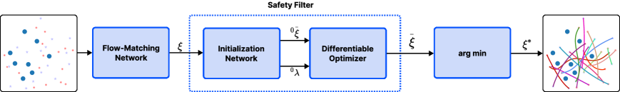
Figure 1: The overview of our multi-robot trajectory pipeline. It has two core components: a trained flow policy and a safety-filter. The trained flow policy takes in start and goal positions of the robots and static obstacle placements (additionally, velocity for dynamic obstacles) and outputs a distribution of trajectories, $\boldsymbol{\xi}$. The multiple flow sampled trajectories are refined in parallel through a safety-filter, and the trajectory with the lowest constraint residual and smoothness is output as the optimal solution. Our SF is accelerated by an initialization network that is conditioned on the samples drawn from the flow policy

II Problem Formulation

Notations

We will use normal-font letters to represent scalars. The vectors and matrices will be represented by bold-faced lower and uppercase, respectively.

TABLE I: Summary of Notation

Symbol	Meaning
$t$	Time-scale of flow ODEs
$k$	Time-step of robot trajectory
$n$	Number of robots
$n_{\text{obs}}$	Number of obstacles in the environment
$n_{d}$	Workspace dimension ($n_{d}\in\{2,3\}$ for 2D/3D)
$(\frac{a}{2},\frac{a}{2},\frac{b}{2})$	Robot Dimension modeled as spheroid
$(a_{o},a_{o},b_{o})$	Obstacle dimension inflated by the robot size.
$n_{\xi}$	Order of polynomial basis for trajectory representation
$S$	Flow model hyperparameter: Trajectory sequence length
$\left[\boldsymbol{\xi}_{i,x},\boldsymbol{\xi}_{i,y},\boldsymbol{\xi}_{i,z}\right]$	Polynomial trajectory basis for $i^{th}$ robot
$q$	Flow model hyperparameter: Obstacle sequence length
$D$	Flow model hyperparameter: DiT embedding size

II-A Trajectory Optimization

We assume that the robots are modeled as double integrator systems which is expressive enough to model quadrotors [17] and holonomic mobile robots. It is a good approximation for on-road vehicles under a broad-set of conditions [18]. However, our formulation trivially extends to higher-order integrator systems as well. We can leverage the differential flatness property allows to directly plan in the space of trajectories and control inputs can be extracted post-hoc from the trajectory derivative.

Given $n$ number of robots and a planning period $K+1$, let $\mathbf{p}_{{i|k}}$ represent the x-y-z coordinate of the $i^{th}$ robot at time step $k$. The joint trajectory optimization problem can therefore be written as the following quadratically constrained quadratic program:

$$\min_{\mathbf{p}_{i|0:K}}\frac{1}{2}\sum_{i=1}^{n}\sum_{k=0}^{K}{\lVert\ddot{\mathbf{p}}_{i|k}\rVert^{2}_{2}}$$ (1a)

$$\lVert\mathbf{M}_{r}^{-1}\left(\mathbf{p}_{i|k}-\mathbf{p}_{j|k}\right)\rVert^{2}_{2}-\mathbf{1}\geq\mathbf{0},\hskip 14.22636pt\forall k\hskip 8.53581pt\forall i,j$$ (1b)

$$\lVert\mathbf{M}_{o}^{-1}\left(\mathbf{p}_{i|k}-\mathbf{p}_{o,m|k}\right)\rVert^{2}_{2}-\mathbf{1}\geq\mathbf{0},\hskip 14.22636pt\forall k\hskip 8.53581pt\forall i,\forall m$$ (1c)

$$\mathbf{p}_{min}\leq\mathbf{p}_{i|k}\leq\mathbf{p}_{max},\forall i,k$$ (1d)

$$\mathbf{p}_{i|0}=\mathbf{b}_{i,0},\mathbf{p}_{i|K}=\mathbf{b}_{i,K},\forall i$$ (1e)

The cost function (1a) minimizes the sum of squared acceleration magnitudes at each time step. However, we can minimize higher-order derivatives like jerk, snap, etc., without affecting the problem structure. The quadratic inequality (1b) is the inter-robot collision avoidance constraints. We assume that each robot is modeled as an axis-aligned spheroid with radius $(\frac{a}{2},\frac{a}{2},\frac{b}{2})$. Hence, $\mathbf{M}_{r}$ is a $3\times 3$ diagonal matrix formed with $(a,a,b)$. The quadratic inequalities (1c) are the collision avoidance constraints between the $i^{th}$ robot and the $m^{th}$ spheroid obstacle, whose position at time step $k$ is given by $\mathbf{p}_{o,m|k}$. For static obstacles, the position is invariant with respect to time. $\mathbf{M}_{o}$ is a $3\times 3$ diagonal matrix formed with $(a_{o},a_{o},b_{o})$ which captures the obstacle dimension inflated with the robot’s dimension. The affine constraints (1d) present the workspace constraints on the robots’ positions. Finally, the equality constraints (1e) enforce the boundary conditions of the robots’ trajectories.

Remark 1

We intentionally don’t include velocity and acceleration bounds in the optimization formulation to reduce the number of constraints. Instead, we follow [16] and use post-hoc scaling of the time-axis to keep the velocity and acceleration within limits. However, velocity and acceleration bounds can be incorporated without affecting the problem structure.

Polynomial Parametrization

We parametrize the positional trajectory of the $i^{th}$ robot $\mathbf{p}_{i|0:K}$ in the following manner:

$$\mathbf{p}_{i|0:K}=\left[\begin{array}[]{ccc}\mathbf{W}&\mathbf{0}&\mathbf{0}\\ \mathbf{0}&\mathbf{W}&\mathbf{0}\\ \mathbf{0}&\mathbf{0}&\mathbf{W}\end{array}\right]\left[\begin{array}[]{c}\boldsymbol{\xi}_{i,x}\\ \boldsymbol{\xi}_{i,y}\\ \boldsymbol{\xi}_{i,z}\end{array}\right]=\overline{\mathbf{W}}\mathbf{c}_{i},$$ (2)

where, $\mathbf{W}$ is a matrix formed with the time-dependent polynomial basis functions and the $\left[\boldsymbol{\xi}_{i,x},\boldsymbol{\xi}_{i,y},\boldsymbol{\xi}_{i,z}\right]$ is a vector of coefficients that define the trajectory. The velocities and accelerations can also be expressed in terms of the coefficients through the time-dependent matrix $\dot{\overline{\mathbf{W}}}$, $\ddot{\overline{\mathbf{W}}}$

We roll the coefficients of all the robots together into a single vector $\boldsymbol{\xi}=(\boldsymbol{\xi}_{1,x},\dots,\boldsymbol{\xi}_{n,x},\boldsymbol{\xi}_{1,y},\dots,\boldsymbol{\xi}_{n,y},\boldsymbol{\xi}_{1,z},\dots,\boldsymbol{\xi}_{n,z})$. Consequently, using (2), we can rewrite the optimization problem into the following more compact form:

$$\underset{\boldsymbol{\xi}}{\text{minimize}} \hskip 14.22636pt\frac{1}{2}\boldsymbol{\xi}^{\top}\mathbf{Q}\,\boldsymbol{\xi}+\mathbf{q}^{\top}\boldsymbol{\xi}$$ (3)

subject to $$\hskip 14.22636pt\mathbf{A}\,\boldsymbol{\xi}=\mathbf{b}$$

$$\hskip 14.22636pt\mathbf{G}\,\boldsymbol{\xi}\leq\mathbf{h}$$

$$\hskip 14.22636pt\mathbf{g}\left(\boldsymbol{\xi}\right)\leq\mathbf{0}$$

where the matrices $\mathbf{Q},\mathbf{A},\mathbf{G}$ and vectors $\mathbf{q},\mathbf{b},\mathbf{h}$ are constants. The affine equality constraints stem from the boundary constraints (1e). The affine inequality models the workspace constraints (1d). The function $\mathbf{g}$ contains the inequalities (1b)-(1c), expressed in terms of polynomial coefficients.

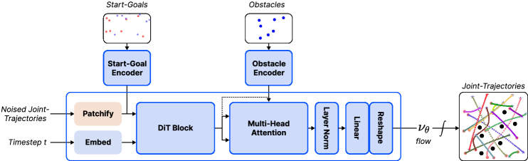
Figure 2: Architecture of our Flow Matching Network. Start-goal and obstacle encoders are based on PointNet++ to ensure invariance to the shuffling of obstacle coordinates and start and goal pairs.

III Method

We present Flow-Opt that combines the generative abilities of the flow-matching policy with a learned differentiable trajectory optimizer for performing centralized multi-robot trajectory optimization in a scalable manner. An overview of our pipeline is shown in Fig.1. The flow policy takes in pairs of start and goal positions and generates a distribution of potential trajectory candidates. We ensure permutation invariance in our flow network architecture so that the trajectory distribution remains invariant to the shuffling of start and goal pairs or obstacle placement in the input data. The trajectories sampled from the learned flow policy may not completely satisfy the collision-avoidance constraints stemming from obstacles in the environment or the inter-robot interaction. Thus, they are refined through a trajectory optimizer, which we refer to in this work as the SF. A key novelty of our SF is that it utilizes a neural network conditioned on the flow trajectories to produce good initializations for the underlying optimization solver. Moreover, this initialization network can be trained purely in a self-supervised manner.

In the remaining sub-sections, we provide details on each of the building blocks of Fig.1.

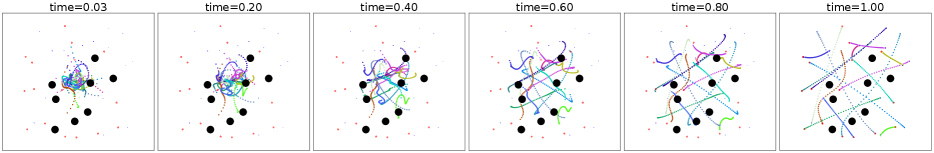
Figure 3: Process of denoising random noise to feasible multi-robot trajectories through a flow policy.

III-A Context-Aware Conditional Flow Matching for Trajectories

We aim to learn a generative model that can produce samples $\boldsymbol{\xi}$ from the conditional distribution $q(\boldsymbol{\xi}|\mathbf{c})$. We treat each trajectory coefficient $\boldsymbol{\xi}$ as a single point in a high-dimensional space. The core idea is to construct a continuous-time flow that transforms samples from a simple, tractable base distribution $p_{0}(\boldsymbol{\xi})$ into samples from our target conditional distribution $q(\boldsymbol{\xi}|\mathbf{c})$.

III-A1 The Conditional Probability Path

We define a time-dependent conditional probability path $p_{t}(\boldsymbol{\xi}|\mathbf{c})$ for $t\in[0,1]$ that connects the base distribution $p_{0}(\boldsymbol{\xi})$ (which is independent of $\mathbf{c}$) to the target distribution $p_{1}(\mathbf{x}|\mathbf{c})=q(\boldsymbol{\xi}|\mathbf{c})$. This path is generated by a conditional vector field $u_{t}(\boldsymbol{\xi}|\mathbf{c})$. The evolution of samples along this path is described by the following ordinary differential equation (ODE):

$$\frac{d\boldsymbol{\xi}_{t}}{dt}=u_{t}(\boldsymbol{\xi}_{t}|\mathbf{c})\quad\text{where}\quad\boldsymbol{\xi}_{0}\sim p_{0}(\mathbf{x}).$$ (4)

If we solve this ODE from $t=0$ to $t=1$, the resulting point $\boldsymbol{\xi}_{1}$ will be a sample from the target distribution $q(\boldsymbol{\xi}|\mathbf{c})$. Please note that the time-sclae of ODE (4) is different from the planning horizon of the robot trajectories. The goal of flow matching is to train a neural network $v_{\theta}(\boldsymbol{\xi}_{t},t,\mathbf{c})$, parameterized by weights $\boldsymbol{\theta}$, to approximate this unknown ground-truth vector field $u_{t}(\boldsymbol{\xi}|\mathbf{c})$.

III-A2 The Conditional Flow Matching Objective

Instead of simulating the ODE, which is intractable for an unknown $u_{t}$, Flow Matching provides a direct regression objective. Given a sample trajectory $\boldsymbol{\xi}_{1}$ from our dataset $q(\boldsymbol{\xi}|\mathbf{c})$ and a sample $\boldsymbol{\xi}_{0}$ from the prior $p_{0}(\boldsymbol{\xi})$, we can construct a path between them. A common and effective choice is a simple linear interpolation:

$$\boldsymbol{\xi}_{t}=(1-t)\boldsymbol{\xi}_{0}+t\boldsymbol{\xi}_{1}.$$ (5)

The ”ground truth” conditional vector field that generates this specific straight-line path is simply the difference between the endpoint and the starting point:

$$u_{t}(\boldsymbol{\xi}_{t}|\mathbf{c})=\boldsymbol{\xi}_{1}-\boldsymbol{\xi}_{0}.$$ (6)

This provides a direct regression target for our neural network $v_{\theta}$. The Conditional Flow Matching (CFM) objective is to minimize the expected squared distance between the network’s prediction and this ground-truth vector field over all possible times, contexts, initial points, and target trajectories:

$$\mathcal{L}_{\text{CFM}}(\theta)=\mathbb{E}_{t\sim\mathcal{U}(0,1),\boldsymbol{\xi}_{0}\sim p_{0}(\boldsymbol{\xi}),(\boldsymbol{\xi}_{1},\mathbf{c})\sim q(\boldsymbol{\xi},\mathbf{c})}\left[\left\|v_{\theta}((1-t)\boldsymbol{\xi}_{0}+t\boldsymbol{\xi}_{1},t,\mathbf{c})-(\boldsymbol{\xi}-\boldsymbol{\xi}_{0})\right\|^{2}\right].$$ (7)

Here, $q(\boldsymbol{\xi},\mathbf{c})$ represents the joint distribution of optimal trajectories and their corresponding contexts from our dataset, and $\mathcal{U}(0,1)$ is the uniform distribution over the time interval. The neural network $v_{\theta}$ is trained to predict the direction $(\boldsymbol{\xi}_{1}-\boldsymbol{\xi}_{0})$ given the interpolated point $\boldsymbol{\xi}_{t}$, the time $t$, and the context $\mathbf{c}$.

III-A3 Generating Novel Trajectories (Inference)

Once the neural network $v_{\theta}$ has been trained by minimizing the objective $\mathcal{L}_{\text{CFM}}$, it approximates the true vector field that maps the prior distribution to the data distribution. To generate a new trajectory for a novel context $\mathbf{c}_{\text{new}}$, we can now solve the learned ODE.

First, we sample an initial point from the prior distribution:

$$\boldsymbol{\xi}_{0}\sim p_{0}(\boldsymbol{\xi}).$$

Then, we solve the following initial value problem from $t=0$ to $t=1$ using a numerical ODE solver (e.g., Euler or Runge-Kutta methods):

$$\frac{d\boldsymbol{\xi}_{t}}{dt}=v_{\theta}(\boldsymbol{\xi}_{t},t,\mathbf{c}_{\text{new}}).$$ (8)

The solution at $t=1$, denoted as $\boldsymbol{\xi}_{1}$, is a novel trajectory coefficient sample ${\boldsymbol{\xi}}$ that is conditioned on the provided context $\mathbf{c}_{\text{new}}$:

$$\boldsymbol{\xi}=\boldsymbol{\xi}_{1}=\boldsymbol{\xi}_{0}+\int_{0}^{1}v_{\theta}(\boldsymbol{\xi}_{t},t,\mathbf{c}_{\text{new}})\,dt.$$ (9)

This process allows us to generate a diverse set of optimal trajectories by starting from different random samples $\boldsymbol{\xi}_{0}$ while keeping the context $\mathbf{c}_{\text{new}}$ fixed. Moreover, we can generate all these diverse trajectories by evaluating (9) in a batch (parallelized) fashion. A typical flow policy trajectory generation is shown in Fig.3.

III-A4 Flow Network Architecture

Our architecture processes noised joint trajectories represented here as $\boldsymbol{\xi}_{t}\in\mathbb{R}^{n_{\xi}\times n\times n_{d}}$, where $n_{\xi}$ denotes the order of polynomial basis functions used for representing the trajectories, $n$ is the number of robots, $n_{d}$ represents the workspace dimension (2D or 3D), and $t\in[0,1]$ indicates the flow timestep. These trajectories are derived through the noise perturbation process described in Eq. (5). The model employs a Diffusion Transformer (DiT) as a backbone.

We employ a CNN based encoder that takes in $\boldsymbol{\xi}_{t}$ and performs a patchification [19] to convert it into a sequence $\boldsymbol{\xi}_{t}^{{}^{\prime}}\in\mathbb{R}^{S\times D}$ of length $S$ and dimension $D$. $S$ and dimension $D$ are tunable model hyperparameters controlling the sequence length and embedding dimension, respectively. We add to $\boldsymbol{\xi}_{t}^{{}^{\prime}}$ sinusoidal positional embeddings to preserve spatial-temporal relationships. Concurrently, the scalar timestep $t$ is encoded into a $D$-dimensional vector $\mathbf{t}^{{}^{\prime}}\in\mathbb{R}^{D}$ using the same sinusoidal embedding scheme, enabling the model to condition on the flow matching process timing.

Contextual information is incorporated through two permutation-invariant PointNet-based networks [20]. One pointnet-based model for start-goal condition $\mathbf{c}_{sg}\in\mathbb{R}^{n\times(2\cdot n_{d})}$ representing start and goal positions for each $n$ agent. The second pointnet-based model is for the obstacle condition $\mathbf{c}_{ob}\in\mathbb{R}^{n_{obs}\times(2\cdot n_{d})}$ representing the obstacle position and velocity, and $n_{obs}$ denotes the number of obstacles. They both form the conditioning inputs $\mathbf{c}=[\mathbf{c}_{sg},\mathbf{c}_{ob}]$ for the flow-matching trajectory prediction network. Both networks maintain invariance to positional shifts in agent start-goal or obstacle state pairs. Each PointNet has $2\cdot n_{d}$ input channels and employs 1D convolutions with a kernel size of 1 within its layers. The two condition networks each produce compact feature representations $\mathbf{c}_{sg}^{{}^{\prime}}\in\mathbb{R}^{S\times D}$ and $\mathbf{c}_{ob}^{{}^{\prime}}\in\mathbb{R}^{q\times D}$ respectively, where $q$ is a tunable parameter for obstacle features.

The core DiT block processes the trajectory embedding $\boldsymbol{\xi}_{t}^{{}^{\prime}}$ conditioned on both the timestep encoding $\mathbf{t}^{{}^{\prime}}$ and start-goal features $\mathbf{c}_{sg}^{{}^{\prime}}$, producing an intermediate representation $\boldsymbol{\xi}^{dit}_{t}\in\mathbb{R}^{S\times D}$. This output then undergoes either self-attention (for obstacle-free cases) or cross-attention with obstacle features $\mathbf{c}_{ob}^{{}^{\prime}}$ (when obstacles exist). Finally, a feed-forward network with linear and normalization layers transforms and reshapes these features to generate the output trajectories $v_{\theta}(\boldsymbol{\xi}_{t},t,\mathbf{c})\in\mathbb{R}^{n_{\xi}\times n\times n_{d}}$ as defined in Eq. (8).

III-B Fast Inference-Time Refinement

The flow policy of the previous subsection is trained purely over demonstrations of optimal trajectories. Thus, it is unaware of the underlying trajectory level constraints. As a result, the predicted trajectories may not be completely feasible. We achieve constraint satisfaction by modifying the flow predicted trajectories through the following optimization.

$$\underset{\overline{\boldsymbol{\xi}}}{\text{minimize}} \hskip 14.22636pt\frac{1}{2}\left\|\overline{\boldsymbol{\xi}}-\boldsymbol{\xi}\right\|_{2}^{2}$$ (10a)

subject to $$\hskip 14.22636pt\mathbf{A}\,\overline{\boldsymbol{\xi}}=\mathbf{b}$$ (10b)

$$\hskip 14.22636pt\mathbf{G}\,\overline{\boldsymbol{\xi}}\leq\mathbf{h}$$ (10c)

$$\hskip 14.22636pt\mathbf{g}\left(\overline{\boldsymbol{\xi}}\right)\leq\mathbf{0}$$ (10d)

Eqns.(10a)-(10d) is a typical projection problem that aims to compute the closest possible trajectory coefficient to $\boldsymbol{\xi}$ that satisfies the constraints. Inference time refinements are commonly used for diffusion and flow based trajectory predictions [10]. In fact, some works formulate them as projection optimization similar to (10a)-(10d) [21], [13]. However, existing works often under-acknowledges the computational cost of inference-time refinements. For example, often these are several times higher than the computation cost associated with the inference process of diffusion or flow policies [10], [13]. Thus, in this paper, we adopt a learning based approach for improving the computational efficiency of inference time refinements. Specifically, we learn warm-start for (10a)-(10d) conditioned on the flow predicted input $\overline{\boldsymbol{\xi}}$. There are two building blocks of our approach. First, we reformulate the underlying quadratic inequalities in constraint function $\mathbf{g}$ (recall (1b)-(1c)) to express the solution process of (10a)-(10d) in the form of differentiable fixed-point operations. Subsequently, we leverage the differentiability to develop a pipeline that performs end-to-end self-supervised learning for accelerating the convergence of fixed-point operations.

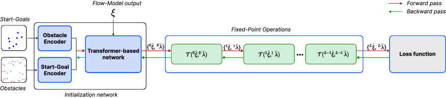
Figure 4: The training pipeline for learning warm-start for the SF solver. The architecture has two components: a learnable part consisting of a start-goal and obstacle encoder and transformer-based network, and a fixed part that resembles $L$ fixed-point iterations of our SF solver. The loss function is simply made of a fixed-point residual. During training, the gradients flow through the fixed-point layer, ensuring the initialization $({{}^{0}}\overline{\boldsymbol{\xi}},{{}^{0}}\overline{\boldsymbol{\lambda}})$ produced by the networks is used by the downstream SF solver. This in turn requires that the fixed-point iterations are differentiable.

.

III-B1 Fixed-Point Representation

We propose a custom SF solver that reduces the solution process of (10a)-(10d) into a fixed-point operation $\mathcal{T}$ of the following form, where the left subscript $l$ denotes the iteration number.

$${{}^{l+1}}{\boldsymbol{\xi}},{{}^{l+1}}\boldsymbol{\lambda}=\mathcal{T}({{}^{l}}{\boldsymbol{\xi}},{{}^{l}}\boldsymbol{\lambda})$$ (11)

We derive the mathematical structure of $\mathcal{T}$ in the Appendix VI, where we also define the Lagrange multiplier $\boldsymbol{\lambda}$. But some interesting points are worth pointing out immediately. First, by carefully reformulating the quadratic inequalities (1b)-(1c), we can ensure that the numerical computations underlying $\mathcal{T}$ only require matrix-matrix products, which can be easily batched and accelerated over GPUs. Secondly, $\mathcal{T}$ involves only differentiable operations, which allows us to compute how changes in the initialization of $\mathcal{T}$ affect the convergence process. This differentiability forms the core of our learning pipeline, designed to accelerate the convergence of fixed-point iteration (11).

III-B2 Learned Initialization for Fixed-Point Iteration

We aim to learn good initializations that accelerate the convergence of the fixed-point iteration (11). A common metric for convergence is the fixed-point residual defined in the following manner [22]

$$\mathcal{L}_{FP}=\left\|\begin{bmatrix}{{}^{l+1}}{\boldsymbol{\xi}}\\ {{}^{l+1}}\boldsymbol{\lambda}\end{bmatrix}-\mathcal{T}({{}^{l}}\overline{\boldsymbol{\xi}},{{}^{l}}\boldsymbol{\lambda})\right\|_{2}^{2}$$ (12)

A good initialization would ensure that the residual (12) quickly converges to zero. To this end, we propose the learning pipeline shown in Fig.4. It consists of a learnable part followed by an unrolled chain of length $L$ of fixed-point iterations. The learnable part consists of encoders for start and goal pairs and environment obstacles. The embeddings from these encoders are paired with the output from a pre-trained flow model $\boldsymbol{\xi}$ and fed to a transformer that produces the warm-start $({{}^{0}}\overline{\boldsymbol{\xi}},{{}^{0}}\boldsymbol{\lambda})$ for the fixed-point iterations. Let ${}^{L}{\overline{\boldsymbol{\xi}}},^{L}\boldsymbol{\lambda}$ be the solution obtained by running the fixed-point iteration for $L$ iterations from the $({{}^{0}}\overline{\boldsymbol{\xi}},{{}^{0}}\boldsymbol{\lambda})$. We formulate the following optimization problem to train the learnable part of the SF.

$$\min_{\boldsymbol{\phi}}\sum_{l=0}^{L-1}\mathcal{L}_{FP}+\left\|{{}^{L}}\overline{{\boldsymbol{\xi}}}-\boldsymbol{\xi}\right\|_{2}^{2},$$ (13)

where $\boldsymbol{\phi}$ contains the weights of the start-goal and obstacle encoders and the transformer network. The first term in (13) minimizes the fixed-point residual at each iteration and is responsible for accelerating the convergence of (11) [22]. The second term ensures that the learned initialization leads to a solution that is minimally displaced from the original flow predicted predicted trajectory coefficient. During training, the gradient of the loss function is traced through the stacked layers of $\mathcal{T}$ to the learnable parts. This ensures that the neural network layers are aware of how its predictions are leveraged by the downstream solver and leads to highly effective warm-start for the fixed-point solver. It is worth pointing out that the loss function (13) does not require the ground-truth solution of the fixed-point iteration (11). In that sense, our learning process is self-supervised and is guided by the fixed-point residual itself.

III-B3 Architecture of Initialization Network

The initialization model is made of two parts: two Pointnet-based models and a lightweight transformer model. The two PointNet encoders (architecturally identical to those in the flow network) generate condition embeddings: $\mathbf{c}_{sg}^{f}\in\mathbb{R}^{S\times 2\cdot n_{d}}$ from start-goal states and $\mathbf{c}_{ob}^{f}\in\mathbb{R}^{q\times 2\cdot n_{d}}$ from obstacles, where $S,q$ are tunable and $n_{d}$ is workspace dimension (2D/3D). The transformer block refines the input flow-generated trajectories $\boldsymbol{\xi}$ conditioned on $\mathbf{c}_{sg}^{f}$ and $\mathbf{c}_{ob}^{f}$.

The trajectories are first patchified via CNN model into $\boldsymbol{\xi}^{{}^{\prime}}\in\mathbb{R}^{S\times D}$ with positional embeddings added. The CNN model used for the patchification is also similar to the one used in the flow model. The transformer layer processes $\boldsymbol{\xi}^{{}^{\prime}}$ with $\mathbf{c}_{sg}^{f}$ via self-attention, optionally applying cross-attention with $\mathbf{c}_{ob}^{f}$ when obstacles exist. The output generates warm-start values: initial Lagrangian multipliers ${}^{0}\overline{\boldsymbol{\lambda}}$ and near-feasible trajectories ${}^{0}\overline{\boldsymbol{\xi}}\in\mathbb{R}^{n_{\xi}\times n\times n_{d}}$ (where $n_{\xi}$ is the polynomial basis order) for the fixed-point operation $\mathcal{T}$ defined in Eq. (11).

IV Connection to Existing Works

In this section, we present a review of closely connected literature and how our approach presented in the previous section fills the key gaps in these works.

IV-A Centralized Trajectory Optimizers

The centralized approach can provide many advantages, such as one-shot feasible trajectory generation between start and goal with a fixed-final time and better trajectory quality due to access to a larger feasible space [18]. This in turn can be crucial for applications such as warehouse automation, where robots need to reach a pickup location in a specified time. Centralized optimizers also find application in drone cinematography [23], drone racing [24], and interaction-aware planning [25], coordination of connected vehicles [18], and target tracking [26]. Moreover, centralized optimizers can provide a framework to generate diverse swarm behaviors crucial for training navigation policies through imitation or reinforcement learning [3].

Given its utility, it is natural to explore ways to make this class of approaches more computationally efficient. Thus, the robotics and control community has shown strong interest in improving the scalability of centralized trajectory optimizers. The underlying idea primarily revolves around decomposing the overall optimization into smaller parallelizable problems. To this end, the Alternate Direction Method of Multipliers (ADMM) has proved to be a useful mathematical tool [27], [28], [29], [30], [31]. ADMM leverages the fact that the only coupling between different robots in optimization (1a)-(1e) stems from the inter-robot collision avoidance constraints (1b). Thus, it breaks down the whole centralized problem into decoupled optimization blocks. Works like [32], [9] explore a different direction for improving scalability: reformulating the computation in a form that can be easily accelerated over GPU cores.

Our Improvement

Our approach provides a substantially faster approach for centralized multi-robot trajectory optimization than the above cited works. One of the main reasons is the computational efficiency of the trajectory optimizer underlying our approach. As shown in Appendix, our optimizer builds upon [9] by incorporating additional constraints for workspace and environment collision. Moreover, we present a batchable version of [9] that can solve several hundred problem instances in parallel in a fraction of a second (see Fig.7).

IV-B Generative Models for Motion Planning

Generative models offer a robust, data-driven approach to motion planning by learning a distribution of expert trajectories, which can either come from human demonstration or through synthetic solvers. While Conditional Variational Autoencoders (CVAEs) [33] are computationally efficient, they can struggle to capture the diverse, multi-modal nature of many planning problems. Vector Quantized Variational Autoencoders (VQ-VAEs) based approaches address this by using a discrete latent space [34] to represent distinct solution types better, though they can be more challenging to train. More recently, diffusion [10], [11], [12] [35], [13], [36] and flow matching policies [37] have become prominent. Both can effectively learn complex, multi-modal trajectory distributions. A unique strength of diffusion and flow policies is that their learned distribution can be adapted at inference times through cost or constraint functions [10], [11]. In that sense, both these approaches can be thought as of learning some prior over the offline datasets of trajectories.

The use of diffusion policies for solving multi-robot motion planning in a centralized manner has only recently been explored, with [12], [13] being the only works, to the best of our knowledge. Authors in [12] learn diffusion priors over the dataset of just single robot motions. At inference times these distributions are steered through the use of conflict-based search algorithms [38]. In contrast, [13] uses the output of [12] to learn the prior over multi-robot trajectories followed by use of trajectory optimization to satisfy safety constraints. The work presented in [36] is somewhat related as it learns diffusion policies over multiple vehicles. However, the focus is on trajectory prediction for autonomous driving, and thus constraint residuals reported in [36] are too high for the learned policy to be used for navigation.

Our Improvement

We present the first application of flow matching for multi-robot motion planning. The inferencing of our flow model is substantially faster than diffusion policy based approaches such as [12], [36], [13]. Moreover, [12], [13] builds upon the unconditional diffusion model of [11]. In contrast, our flow policy explicitly takes in start-goal positions and environment context (recall Fig.2, Section III-A4) , obtained through a permutation invariant encoder.

IV-C Use of Safety Filter (SF)

Predictions from learned neural network models typically struggle to satisfy constraints [39], even though they might have been trained extensively on datasets of feasible trajectories. Thus, it is common to employ a safety filter to perform a correction at the inference time by projecting the predictions from the learned models onto the feasible set [40]. Recently, works like [41], [42] integrates SF with diffusion models to satisfy constraints such as collision avoidance.

Our Improvement

It is often observed in existing works that SF does the heavy lifting in a data-driven pipeline and thus can become computationally heavy. Our approach fully acknowledges this and thus builds a self-supervised learning pipeline (recall Fig.4) to improve the computational efficiency of SF. We are not aware of any existing learning accelerated SF for multi-robot planning.

IV-D Learning to Warm-start Optimization

The performance of non-convex trajectory optimizers depends heavily on the quality of initial guess. Thus, there is a strong case for adopting data-driven approaches to come up with problem specific initialization (warm-start) for the optimizers. The most straightforward approach is to fit some neural network over the dataset of optimal solutions. The predictions from the learned model can then be used to initialize the optimizer [43], [44]. However, in our experience such an approach often do not perform satisfactorily on complicated problems such as multi-robot planning (e.g see Fig.13-14). This is because the trained initialization model is unaware of its predictions is used by the downstream solver. Thus, authors in [22] recommend hybrid architectures like that shown in Fig.4 wherein, the optimizer is embedded along with learnable neural network layers in the training pipeline.

Our Improvement

The end-to-end warm-start learning of [22] has only been applied to convex problems which has two important consequences. First, for these class of problems, the solution process can be easily cast as a chain of differentiable computations. In contrast, off-the-shelf non-convex optimizers often rely on non-differentiable steps such as line-search. Thus, extending [22] to non-convex problems require developing custom end-to-end differentiable solvers. The derivations presented in the Appendix VI precisely fulfill this objective.

Second, the learning pipeline of [22] only considers a fixed-point residual (recall (12)) because convex problems have only one solution. In contrast, we augment the loss with additional terms to find solutions with minimal projection residual (see (13)).

V Validation and Benchmarking

The objective of this section is threefold.

• We demonstrate that our approach is indeed capable of producing smooth multi-robot trajectories in a scalable manner.

• We demonstrate improvement in trajectory quality, success rate, and computation time over existing model-based and data-driven approaches.

• We analyze the robustness of our approach to generalize to both in-distribution and out-of-distribution test cases.

V-A Implementation Details

The flow network of Fig.2, initialization network of Fig.4 and the SF solver were all implemented in JAX [45] with Equinox [46] as the neural training library. The parameters of the network are presented in Appendix, Section VI, Table VI, VII. The flow policy was trained on 20 thousand trajectories that covered start and goal within a rectangular workspace centered at origin.

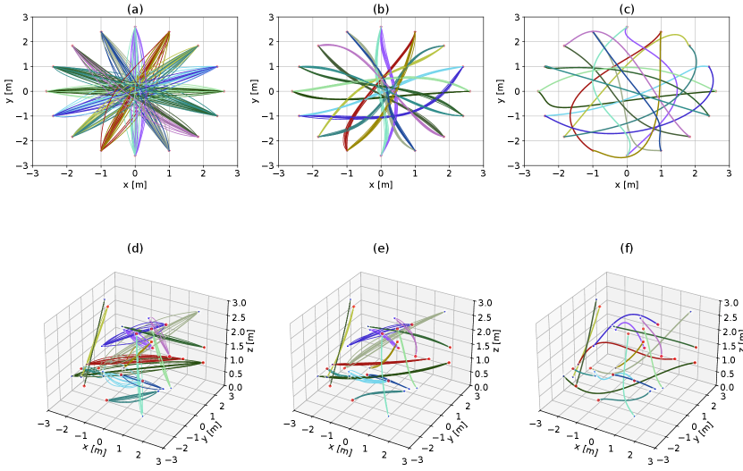
Figure 5: The three stages of our trajectory planning pipeline. We first sample a large number of trajectories ($\approx 256$) from the trained flow policy (Fig.(a), (d)). We then sort the sampled trajectories based on constraint satisfactions and choose the top 10 with the lowest residual (Fig.(b)-(e)). Finally, these trajectories are refined through SF, and the feasible trajectory with the lowest smoothness cost is output as the optimal solution (Fig.(c)-(f)).

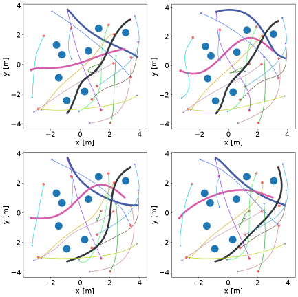
Figure 6: Demonstration of diverse collision avoidance behaviors for 16 robots in obstacle-filled environments obtained with our approach. As can be seen, the same robot can choose different strategies to avoid static obstacles and accordingly also its strategy to avoid other robots. Some of the trajectories showing pronounced diversity are highlighted.

V-B Qualitative Validation

In this subsection, we validate different steps of our pipeline that was presented in Fig.1 on two simple scenarios involving 16 robots (Fig.5). As mentioned earlier, we first sample from the trained flow policy before refining it through SF. We break down the sampling process into two parts. We first sample a large number of trajectories from the flow policy (Fig.5(a),(d)). We then select the top 10 trajectories that show the least constraint violation (Fig.5 (b), (e)) and these are then passed through the SF. The trajectories obtained from the SF are ranked based on constraint residual (see (31)) and smoothness (acceleration norm) and then the best trajectory is returned as the optimal solution (Fig.5 (c), (f)).

It is worth pointing out that our flow policy was trained on trajectories between randomly sampled start and goal pairs. Yet, it could generalize to the unique case where the robots are placed on the perimeter of a circle and have to move to their antipodal position.

A quintessential feature of flow matching is its ability to learn multi-modal distribution. In our context, this would translate to diverse collision avoidance behaviors expressed by the variation in speed and paths of the robots. The diversity in trajectories is particularly pronounced in the presence of static obstacles. Fig.6 shows one such result for a scenario where 16 robots move between their assigned start and goal in a cluttered environment. We highlight some of the trajectories which goes around static obstacles in different ways and accordingly also adapt their strategies for avoiding other robots. In other words, having a dedicated initialization network for warm-starting the SF solver allows us to reach a particular residual threshold at lower iterations than what can be achieved with naively using the flow output

Why is Diversity Important: We envision one of the use-cases of our approach in generating data-driven simulation environments for training navigation policies [1, 2], [47]. The diverse multi-robot trajectories can be used to simulate a rich set of crowd behaviors.

V-C Scalability

A key advantage of our framework is its exceptional computational efficiency, which enables high-throughput trajectory planning by leveraging massive parallelism. We validate this performance in Figure 7, which analyzes the scalability of our pipeline’s two core components. First, the inference speed of our learned flow policy allows for extensive exploration of the solution space. As shown in Figure 7(a), the policy is capable of generating hundreds of candidate trajectories in tens of milliseconds, even for large systems. This rapid generation is fundamental to our approach, as it provides a rich set of high-quality candidates for the refinement stage. Second, our SF solver is designed to capitalize on this parallelism. Figure 7(b) confirms that its computation time scales near-linearly with the number of trajectories refined simultaneously, a direct benefit of our custom GPU-vectorized solver (see VI).

The synergy between rapid sampling and parallel refinement creates a pipeline uniquely suited for solving multiple problems concurrently. For instance, our system can tackle fifty distinct planning problems at once. Generating 10 candidate trajectories for each problem (500 total) takes under 60 ms. Refining the top 5 candidates from each problem (250 total) takes less than 300 ms. Consequently, our framework can deliver high-quality, refined solutions for all fifty problems in well under a second, demonstrating its significant potential for real-time, multi-task applications.

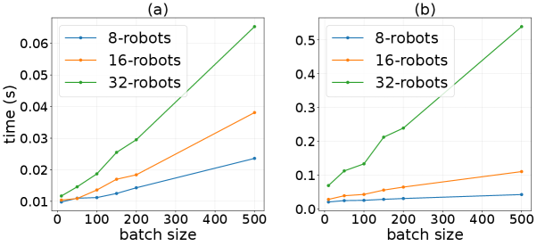
Figure 7: Fig.(a) shows the computation time required to sample a batch of trajectories from the flow model for different number of robots. Fig.(b) shows the computation time to perform 500 iterations of SF to refine a batch of trajectories. As can be seen, due to GPU acceleration/parallelization, both timings scale almost linearly with batch size.

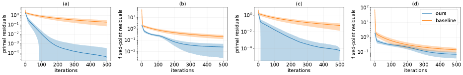
Figure 8: Comparison of primal and fixed-point residuals obtained with baseline [9] and our approach. Fig.(a)-(b) summarizes the trends for 16 robot scenarios in 2D, while Fig.(c)-(d) reproduces the same for a 3D setting. The shaded region presents the confidence interval, while the solid lines depict the mean trend.

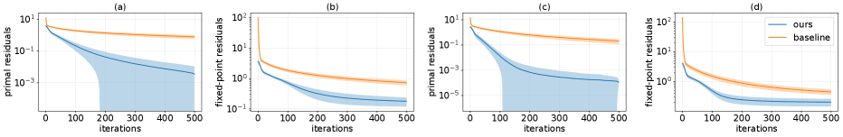
Figure 9: The same results as Fig.8 but reproduced for 32 robot setting in 2D ( Fig.(a)-(b) ) and 3D (Fig.(c)-(d)). The baseline is [9].

TABLE II: Comparison of Primal Results for Baseline [9] and Ours-Init Methods

Scenario	Primal	Baseline			Ours-Init
		mean	max	min	mean	max	min
16 agents 2D	0.01	2606	10987	340	82	464	10
	0.001	4941	14827	667	110	499	10
16 agents 3D	0.01	1102	7921	4	46	228	1
	0.001	2099	9999	4	61	485	1
32 agents 2D	0.01	9747	29758	1991	271	500	84
	0.001	17189	29956	3787	338	500	102
32 agents 3D	0.01	2280	9304	694	100	353	24
	0.001	4190	9999	1289	137	479	27

TABLE III: Combined performance comparison of Baseline [9] and Our method in 2D and 3D planning scenarios.

Dimension	# of robots	Method	Metrics
			time (s)	success rate	smoothness cost ($[m/s^{2}]$)	arc length ($[m]$)
2D	8	Baseline [9]	0.218	100	0.2646	1.2966
		Ours	0.0515	100	0.2141	1.0489
	16	Baseline [9]	0.5927	99.9	0.278	1.3624
		Ours	0.0654	100	0.2398	1.1748
	32	Baseline [9]	3.4068	99.61	0.2027	0.9934
		Ours	0.2966	100	0.241	1.1809
3D	16	Baseline [9]	0.1482	100	0.6313	3.0932
		Ours	0.069	100	0.6272	3.0731
	32	Baseline [9]	0.999	99.81	0.7066	1.154
		Ours	0.1511	100	0.7002	3.4309

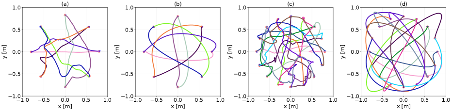
Figure 10: Comparison between our approach and a diffusion-based multi-robot planner MMD [12]. Fig.(a)-(b) shows MMD and our approach in a 8 robot scenario respectively. Fig.(c)-(d) repeats the comparison for 16 robots with Fig.(c) being the MMD and Fig.(d) depicting our approach. As can be seen, our approach models the global interaction between the robots better leading to smoother de-conflicting maneuvers.

TABLE IV: Comparison of MMD [12] and Our Method on 2D Scenarios

Method	Num. of Robots	Time (s)	Success Rate	Smoothness cost ($[m/s^{2}]$)	Arc Length ($[m]$)
MMD	8	5.3706	100	0.2063	1.0155
	16	18.0	100	0.2393	1.1779
	32	48.1758	100	0.2487	1.2239
Ours	8	0.0515	100	0.2141	1.0489
	16	0.0654	100	0.2398	1.1748
	32	0.2966	100	0.2410	1.1809

V-D Comparison with [9]

We compare our hybrid approach that combine aspects of data-driven reasoning and trajectory optimization with a centralized approach that solves the problem from scratch without any learning. To this end, we choose [9] as our baseline as it is very closely related to our work. In fact, the SF solver presented in the Appendix VI builds upon [9] by incorporating additional constraints and augmenting an initialization network. Our analysis focuses on three different aspects:

• Convergence: How fast each approach is able to converge to a trajectory with low fixed-point and primal residuals. The latter is formulated in Eqn. (31), serves as a key metric, quantifying the satisfaction of critical constraints: workspace limits (1d), inter-robot separation (1b), and obstacle avoidance (1c).

• Success-Rate and Computation Time: Given an upper-bound of $10k$ iterations, what is the percentage of problems solved by our approach and [9] and the corresponding computation time?

• Trajectory Quality: The smoothness cost (trajectory acceleration norm) and arc-length associated with trajectories obtained with both methods.

Fig.8-9 shows the decay of primal and fixed-point residuals across iterations for different problem scenarios. As can be seen, our approach delivers substantially faster decay in the residuals by leveraging learning on prior collected datasets. The difference is more pronounced at lower iteration count. To further quantify the performance gain provided by our approach, Table II reports the number of iterations [9] and our approach requires to achieve primal residual values below $0.01$ and $0.001$. This statistic is crucial as it directly corresponds to the speed at which each method can converge to a (approximately) feasible trajectory. Consider the 2D scenario with 16 robots. The mean iteration number needed by our approach to reach a residual of $0.01$ is 82. This is 30 times less than the mean number of iterations required by [9]. The performance gap further widens when we consider the primal residual threshold of $0.001$. Similar trend persists for other planning scenarios summarized in Table II.

Table III compares [9] and our approach in terms of success-rate, computation-time, and trajectory quality. The latter two metrics are very similar for both methods. However, our approach brings major improvement in terms of computation time. For example, for 8 robot planning problems, our approach is four times faster than [9]. The performance gap increases further with an increase in the number of robots. For 16 robot case, our approach is up to an order of magnitude faster in 2D setting and more than two times faster in 3D setting. The 2D robot setting is particularly challenging because of the reduced space maneuvering space available to each robot. In this difficult setting, our approach provides almost an order of magnitude speed-up over [9].

V-E Comparison with Diffusion Based Multi-Robot Planner MMD [12]

In this subsection, we compare our approach with a MMD [12] that leverages diffusion policies and combines with graph search methods to plan multi-robot trajectories. A qualitative comparison is shown in Fig.10 for a scenario where 16 robots are placed on the perimeter of a circle and have to move to their antipodal position. As can be seen, both approaches produce distinctively different kind of trajectories. The MMD produced trajectories lead robots directly to the center of the circle which is the main conflict point in this scenario. Subsequently, the robots coordinate to navigate safely towards the goal. While MMD successfully produced safe trajectories, it does not start de-conflicting un till the robots are very close to each other. This is because the underlying diffusion policy does not capture the multi-robot interactions as it is learned on the dataset of just single robot motions [12]. In contrast, our flow policy can capture global interactions between the robots and chooses a de-conflicting maneuver that results in more clearance between the robots.

To further quantify the benefits that our approach provides in terms of inter-robot clearance, we considered 1000 random 2D planning scenarios with different numbers of robots. We sampled start and goal positions from a rectangular area of $[-1,1]\times[-1,1]$. Each robot had a circular footprint with radius $0.1m$. Fig.11 summarizes the results. It shows the statistics of average pair-wise robot distances obtained with MMD and our approach across different planning benchmarks. As can be seen, in 8 robot planning scenarios, our approach produces close to 16 $\%$ improvement in average inter-robot distances. We notice marginal improvement in 16 robot scenarios, and as the number of robots increases further, the space becomes too cluttered, and both methods eventually provide the same performance. Nevertheless, it can be concluded that if there is more maneuvering space, our approach is more likely to leverage it than MMD.

Table IV compares the overall performance of our approach and MMD in terms of some key metrics: smoothness cost (trajectory acceleration norm) and arc-length. Both approaches show similar average trajectory quality (smoothness cost, arc-length) and success-rate across 1000 different problem instances, each for 8, 16, and 32 robots. However, the computation-time trends are strikingly different. The slow diffusion policy underlying MMD and computationally expensive conflict-search results in much higher computation time than our approach. For example, for the 8 robot scenario, our approach is an order of magnitude faster than MMD. This gap increases to $160$ times across the 32 robot planning instances.

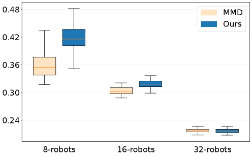
Figure 11: Comparison of inter-robot distances resulting from MMD [12] and our approach. If free space is available, as in the case of 8 and 16 robot planning problems, our approach can find trajectories with higher clearance between the robot trajectories. As the number of robots increases and space becomes restrictive, both approaches converge to similar behavior.

V-F Comparison with [16]

In this subsection, we benchmark our approach against [16], which employs a batch-sequential planning strategy. This method first partitions the robots into distinct groups. For each group, it performs joint trajectory planning, considering all robots within that specific group simultaneously. Following this initial grouping and intra-group planning, the approach transitions to a sequential planning phase to coordinate the actions between the different groups. This means that the groups have a predetermined order, and the trajectory planning for each group is carried out one by one. A significant characteristic of this method is that each group must treat all previously planned groups as dynamic obstacles.

A qualitative comparison between our approach and [16] is shown in Fig.12. We consistently observed that [16] produced longer and more curved paths. This is because the sequential approach of Fig.12 restricts the potential for more complex and cooperative group interactions. For instance, a group planned later in the sequence cannot influence the trajectory of a group planned earlier, even if a slight adjustment could lead to a more globally optimal or efficient solution for the entire multi-robot team. In contrast, our approach considers the inter-robot interaction more efficiently by searching in the joint feasible space of all the robots.

Table V further reinforces the trend observed in Fig.12. Across 16 and 32 robot planning instances, our approach achieved $33\%$ and $29\%$ shorter trajectories, respectively. The restricted planning space available to [16] also affects its success rate, which is $89\%$ and $69\%$ for 16 and 32 robot planning problems, respectively. In contrast, our approach successfully solves every problem in this benchmarking. Our approach is also almost an order of magnitude faster than [16] across all problem instances.

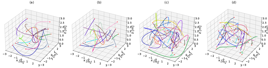
Figure 12: Comparison between our approach and [16]. Fig.(a)-(b) considers the 3D planning scenario involving 16 robots with (a) being [16] and Fig.(b) depicting our approach. Similarly, Fig.(c) and (d) show [16]’s and our performance, respectively, while planning for 32 robots in 3D. It can be seen that our approach produces less curved trajectories, which follow a shorter path between the start and goal.

TABLE V: Performance comparison of our proposed method against [16] in 3D environments for 16 and 32 robots.

	[16] on 3D			Ours on 3D
Num. of Robots	Time (s)	Success Rate (%)	Arc Length ($[m]$)	Time (s)	Success Rate (%)	Arc Length ($[m]$)
16	0.54	89.89	4.0669	0.069	100	3.0731
32	1.72	63.12	4.4407	0.1511	100	3.4309

V-G Ablations and Additional Results

V-G1 Importance of a Initialization Network in SF Convergence

We now analyze the critical role of our flow-conditioned initialization network in warm-starting the SF solver. To do so, we perform an ablation study where we bypass this network and initialize the SF solver directly with the output from the flow policy. This experiment tests whether the near-optimal trajectories produced by the flow policy are a sufficient initial guess for robust convergence. This direct approach is significantly less effective as shown in Figures 13 and 14. The decay of both the primal and fixed-point residuals is substantially slower than our full model, including the initialization network. This outcome highlights a key design insight: the flow policy and the SF solver have distinct objectives. The flow policy is trained solely to imitate expert data and is therefore agnostic to the optimization landscape of the downstream solver. In contrast, the initialization network is explicitly trained to bridge this divide. It learns to refine the flow policy’s output, transforming it into a starting point that is not just near-optimal in trajectory space, but is also a more effective initial guess for the SF solver’s specific optimization process.

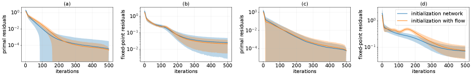
Figure 13: Primal and fixed-point residuals for the SF solver for 16 robot planning problem in (2D) (Fig.(a)-(b)) and 3D (Fig. (c)-(d)). We show the trend for two different initialization strategies: one where the SF solver is directly initialized with the flow policy output and in the second, it is warm-started using the initialization network conditioned on the flow policy output. It can be seen that having a dedicated initialization network leads to a faster decay of primal and fixed-point residuals.

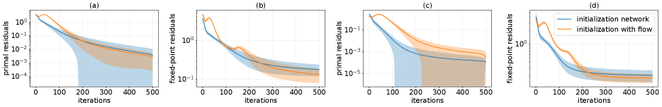
Figure 14: Primal and fixed-point residuals for the SF solver for 32 robot planning problem in (2D) (Fig.(a)-(b)) and 3D (Fig. (c)-(d)). The results carry similar meaning as Fig.13.

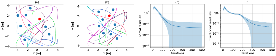
Figure 15: We evaluate the robustness of the SF solver under out-of-distribution test-time perturbations. Specifically, the initialization network of SF is trained with a fixed number of obstacles (eight in our case, shown in cyan). However, during testing, we included an additional obstacle. As seen from Fig.(a)-(b), the SF is resilient to an increase in the number of obstacles and can successfully produce smooth and feasible trajectories. Fig.(c)-(d) further demonstrates the resilience; the primal and fixed-point residual decay is still close to the unperturbed setting shown in Fig.8.

V-G2 Adaptation to Perturbation in Problem Parameters

Our initialization network is trained on environments with a fixed number of obstacles, raising a critical question: can it generalize to novel problem configurations at inference time? To evaluate this robustness, we designed test scenarios where we introduced an additional obstacle that was not present during the training phase (Figures 15(a)-(b)). Despite this out-of-distribution perturbation, our SF solver competes strongly, successfully computing smooth and feasible trajectories. This qualitative success is corroborated by quantitative analysis, as shown in Figures 15(c)-(d). The rapid decay of the primal and fixed-point residuals confirms that the solver maintains its efficient convergence, underscoring its robustness to unforeseen environmental changes.

VI Appendix

VI-A Derivation of Fixed-Point Iteration Form

The following derivation builds upon [9] but improves it in the following manner.

• Inclusion of obstacle avoidance and workspace constraints without disturbing the underlying numerical structure.

• Exposing the optimizer steps as a batchable and GPU-accelerated fixed-point iteration.

We begin by reformulating the quadratic inequalities contained in the constraint function $\mathbf{g}$

VI-A1 Quadratic Constraints in Spherical Form

The inter-robot collision avoidance constraints (1b) can be re-phrased into the following spherical form.

$$\mathbf{p}_{i|k}-\mathbf{p}_{j|k}=d_{ij|k}\begin{bmatrix}a\cos\alpha_{ij|k}\sin\beta_{ij|k}\\ a\sin\alpha_{ij|k}\sin\beta_{ij|k}\\ b\cos\beta_{ij|k}\end{bmatrix},1\leq d_{ij|k}\leq\infty,$$ (14)

where $\alpha_{ij|k},\beta_{ij|k}$ and $d_{ij|k}$ are the spherical angles and normalized line of sight-distance between the agents. These are unknown and will be obtained by the SF optimizer along with other variables. We recall that the agents are modeled as spheroids with dimension $(\frac{a}{2},\frac{a}{2},\frac{b}{2})$

Following a similar notation, we can rewrite the obstacle avoidance constraints (1c) in the following manner.

$$\mathbf{p}_{i|k}-\mathbf{p}_{o,m|k}=d_{o,m|k}\begin{bmatrix}a_{o}\cos\alpha_{o,m|k}\sin\beta_{o,m|k}\\ a_{o}\sin\alpha_{o,m|k}\sin\beta_{o,m|k}\\ b_{o}\cos\beta_{o,m|k}\end{bmatrix},$$

$$1\leq d_{o,m|k}\leq\infty.$$ (15)

VI-A2 Reformulated Problem

We now get the following reformulation of the SF optimizer(10a)-(10d), obtained by replacing (10d) with (19) derived from (14)-(15).

$$\min_{\overline{\boldsymbol{\xi}},\tilde{\boldsymbol{\alpha}},\tilde{\boldsymbol{\beta}},\tilde{\mathbf{d}}}\frac{1}{2}\left\|\overline{\boldsymbol{\xi}}-{\boldsymbol{\xi}}\right\|_{2}^{2}$$ (16)

$$\mathbf{A}\overline{\boldsymbol{\xi}}=\mathbf{b}$$ (17)

$$\mathbf{G}\overline{\boldsymbol{\xi}}\leq\mathbf{h}$$ (18)

$$\mathbf{F}\overline{\boldsymbol{\xi}}=\mathbf{e}(\tilde{\boldsymbol{\alpha}},\tilde{\boldsymbol{\beta}},\tilde{\mathbf{d}})$$ (19)

$$\mathbf{d}_{min}\leq\tilde{\mathbf{d}}\leq\mathbf{d}_{max}$$ (20)

$${\textbf{F}}=\hskip-4.26773pt\begin{bmatrix}\begin{bmatrix}\mathbf{F}_{r}\\ \mathbf{F}_{o}\end{bmatrix}\hskip-7.11317pt&\hskip-7.11317pt\textbf{0}\hskip-7.11317pt&\hskip-7.11317pt\textbf{0}\\ \textbf{0}\hskip-7.11317pt&\hskip-7.11317pt\hskip-4.26773pt\begin{bmatrix}\mathbf{F}_{r}\\ \mathbf{F}_{o}\end{bmatrix}\hskip-7.11317pt&\hskip-7.11317pt\textbf{0}\\ \textbf{0}\hskip-7.11317pt&\hskip-7.11317pt\textbf{0}\hskip-7.11317pt&\hskip-7.11317pt\begin{bmatrix}\mathbf{F}_{r}\\ \mathbf{F}_{o}\end{bmatrix}\end{bmatrix}\hskip-4.26773pt,{\mathbf{e}}=\hskip-4.26773pt\begin{bmatrix}a\mathbf{d}\cos{\boldsymbol{\alpha}}\sin{\boldsymbol{\beta}}\\ \mathbf{x}_{o}+a_{o}\mathbf{d}_{o}\cos{\boldsymbol{\alpha}_{o}}\sin{\boldsymbol{\beta}_{o}}\\ a\mathbf{d}\sin{\boldsymbol{\alpha}}\sin{\boldsymbol{\beta}}\\ \mathbf{y}_{o}+a_{o}\mathbf{d}_{o}\sin{\boldsymbol{\alpha}_{o}}\sin{\boldsymbol{\beta}_{o}}\\ b\hskip 2.84544pt\mathbf{d}\cos{\boldsymbol{\beta}}\\ \mathbf{z}_{o}+b_{o}\mathbf{d}_{o}\cos{\boldsymbol{\beta}_{o}}\end{bmatrix}\hskip-4.26773pt,$$ (21)

$\tilde{\boldsymbol{\alpha}}=(\boldsymbol{\alpha},\boldsymbol{\alpha}_{o})$, $\tilde{\boldsymbol{\beta}}=(\boldsymbol{\beta},\boldsymbol{\beta}_{o})$, $\tilde{\mathbf{d}}=(\mathbf{d},\mathbf{d}_{o})$. The $\boldsymbol{\alpha}$ is formed by stacking $\alpha_{ij|k}$ for all agent pairs $(i,j)$ and all time step $k$. Similarly, $\boldsymbol{\alpha}_{o}$ is formed by stacking $\alpha_{o,m|k}$ for all $m$ and $k$. We follow similar construction for $\boldsymbol{\beta}$, $\boldsymbol{\beta}_{o}$, $\mathbf{d}$, and $\mathbf{d}_{o}$. Let $(x_{o,m|k},y_{o,m|k},z_{o,m|k})$ be the components of obstacle position $\mathbf{p}_{o,m|k}$. Then, $\mathbf{x}_{o}$, $\mathbf{y}_{o}$, $\mathbf{z}_{o}$ are formed by stacking the respective values for all $m$ and $k$.

$$\mathbf{F}_{r}=\begin{bmatrix}\mathbf{F}_{r,1}\\ \mathbf{F}_{r,2}\\ \vdots\\ \mathbf{F}_{r,n-1}\end{bmatrix}\otimes\mathbf{P},\hskip 18.49988pt\mathbf{F}_{o}=\begin{bmatrix}\mathbf{P}&&\\ &\ddots&\\ &&\mathbf{P}\end{bmatrix}$$ (22)

$$\mathbf{F}_{r,i}=\begin{bmatrix}\mathbf{F}_{i}&-\mathbf{I}\end{bmatrix},\mathbf{F}_{i}=\begin{bmatrix}\mathbf{0}_{n-i\times 1}&\mathbf{0}_{n-i\times 1}&\dots&{\mathbf{1}_{n-i\times 1}}\end{bmatrix}_{n-i\times i}$$ (23)

The matrix $\mathbf{F}_{o}$ is a block-diagonal matrix with a number of blocks equal to the number of robots. The matrix $\mathbf{F}_{i}$ is formed with $i-1$ blocks of $n-i$ length zero vector and a single vector of ones at the $i^{th}$ column, where $n$ is the number of robots. The symbol $\otimes$ represent the Kronecker product.

VI-A3 Solution Process

We relax the non-convex equality (19) and affine inequality constraints as penalties and augment them into the cost function using the Augmented Lagrangian method

$$\mathcal{L}=\frac{1}{2}\left\|\overline{\boldsymbol{\xi}}-{\boldsymbol{\xi}}\right\|_{2}^{2}+\frac{\rho}{2}\left\|\mathbf{F}\overline{\boldsymbol{\xi}}-\mathbf{e}(\tilde{\boldsymbol{\alpha}},\tilde{\boldsymbol{\beta}},\tilde{\mathbf{d}})\right\|_{2}^{2}+\frac{\rho}{2}\left\|\mathbf{G}\overline{\boldsymbol{\xi}}-\mathbf{h}+\mathbf{s}\right\|_{2}^{2}-\langle\boldsymbol{\lambda},\overline{\boldsymbol{\xi}}\rangle,$$ (24)

where $\rho$ is a known constant, the variable $\boldsymbol{\lambda}$ are so-called Lagrange multipliers and $\mathbf{s}$ is an unknown positive slack variable. We minimize (24) subject to (17) through an Alternating Minimization (AM) approach, wherein at each step, only one variable group among $\overline{\boldsymbol{\xi}},\tilde{\boldsymbol{\alpha}},\tilde{\boldsymbol{\beta}},\tilde{\mathbf{d}}$ is optimized while others are held fixed. Specifically, the AM routine decomposes into the following iterative steps, wherein the left superscript $l$ tracks the values of a variable across iterations. For example, ${{}^{l}}\overline{\boldsymbol{\xi}}$ is the value of $\overline{\boldsymbol{\xi}}$ at iteration $l$.

$${{}^{l+1}}\tilde{\boldsymbol{\alpha}} =\operatorname*{arg\,min}_{\tilde{\boldsymbol{\alpha}}}\mathcal{L}({{}^{l}}\overline{\boldsymbol{\xi}},\tilde{\boldsymbol{\alpha}},{{}^{l}}\tilde{\boldsymbol{\beta}},{{}^{l}}\tilde{\mathbf{d}},{{}^{l}}\boldsymbol{\lambda})=f_{1}({{}^{l}}\overline{\boldsymbol{\xi}})$$ (25a)

$${{}^{l+1}}\tilde{\boldsymbol{\beta}} =\operatorname*{arg\,min}_{\tilde{\boldsymbol{\beta}}}\mathcal{L}({{}^{l}}\overline{\boldsymbol{\xi}},{{}^{l+1}}\tilde{\boldsymbol{\alpha}},\tilde{\boldsymbol{\beta}},{{}^{l}}\tilde{\mathbf{d}},{{}^{l}}\boldsymbol{\lambda})=f_{2}({{}^{l}}\overline{\boldsymbol{\xi}})$$ (25b)

$${{}^{l+1}}\tilde{\mathbf{d}} =\operatorname*{arg\,min}_{\mathbf{d}_{min}\leq\tilde{\mathbf{d}}\leq\mathbf{d}_{max}}\mathcal{L}({{}^{l}}\overline{\boldsymbol{\xi}},{{}^{l+1}}\tilde{\boldsymbol{\alpha}},{{}^{l+1}}\tilde{\boldsymbol{\beta}},\tilde{\mathbf{d}},{{}^{l}}\boldsymbol{\lambda})=f_{3}({{}^{l}}\overline{\boldsymbol{\xi}})$$ (25c)

$${{}^{l+1}}\mathbf{s} =\max(0,-\mathbf{G}{{}^{l}}\overline{\boldsymbol{\xi}}-\mathbf{h})$$ (25d)

$${{}^{l+1}}\boldsymbol{\lambda} ={{}^{l}}\boldsymbol{\lambda}-\rho\mathbf{F}^{T}\mathbf{r}_{1}-\rho\mathbf{G}^{T}\mathbf{r}_{2}$$ (25e)

$${{}^{l+1}}\overline{\boldsymbol{\xi}} =\operatorname*{arg\,min}_{\mathbf{A}\overline{\boldsymbol{\xi}}=\mathbf{b}}\mathcal{L}(\overline{\boldsymbol{\xi}},{{}^{l+1}}\mathbf{e},{{}^{l+1}}\boldsymbol{\lambda})$$ (25f)

$$=\mathbf{M}^{-1}\boldsymbol{\eta}$$ (25g)

$${{}^{l+1}}\mathbf{e}=\mathbf{e}({{}^{l+1}}\tilde{\boldsymbol{\alpha}},{{}^{l+1}}\tilde{\boldsymbol{\beta}},{{}^{l+1}}\tilde{\mathbf{d}})$$ (26)

$$\mathbf{r}_{1}=\mathbf{F}{{}^{l}}\boldsymbol{\xi}-{{}^{l+1}}\mathbf{e},\hskip 18.49988pt\mathbf{r}_{2}=\mathbf{G}{{}^{l}}\overline{\boldsymbol{\xi}}-\mathbf{h}+{{}^{l+1}}\mathbf{s}$$ (27)

$$\textbf{M}=\begin{bmatrix}\mathbf{I}+\rho\mathbf{F}^{T}\mathbf{F}&\textbf{A}^{T}\\ \mathbf{A}&\mathbf{0}\end{bmatrix}^{-1}\hskip-5.40608pt,\boldsymbol{\eta}=\begin{bmatrix}\rho\mathbf{F}^{T}\hskip 2.84544pt{{}^{l+1}}\mathbf{e}+{{}^{l+1}}\boldsymbol{\lambda}+{\boldsymbol{\xi}}\\ \mathbf{b}\end{bmatrix}$$ (28)

The minimization (25a)-(25c) have a closed-form solution which can be expressed as a function of ${{}^{l}}\overline{\boldsymbol{\xi}}$ [9]. For example, one part of minimization (25a) reduces to

$${{}^{l+1}}\alpha_{ij|k}=\arctan 2({{}^{l}}y_{i|k}-{{}^{l}}y_{j|k},{{}^{l}}x_{i|k}-{{}^{l}}x_{j|K}),\forall i,j,k$$ (29)

where $({{}^{l}}x_{i|k},{{}^{l}}y_{i|k})$ are the components of the position ${{}^{l}}\mathbf{p}_{i|k}$ and are completely characterized by the trajectory coefficient ${{}^{l}}\overline{\boldsymbol{\xi}}$ at iteration $l$ of the AM optimizer.

Similarly, (25f) is simply an equality-constrained QP and thus has an explicit formula for its solution. Moreover, since ${{}^{l+1}}\mathbf{e}$ and ${{}^{l+1}}\boldsymbol{\lambda}$ are explicit functions of ${{}^{l}}\overline{\boldsymbol{\xi}}$, ${{}^{l}}\boldsymbol{\lambda}$, (25e)-(25f) constitutes the fixed-point iteration $\mathcal{T}$ presented in (11).

A few points about the AM steps are worth noting.

• Differentiability: Since every step has a closed-form solution, we can easily unroll them into a differentiable computational graph.

• Steps (25a)-(25e) do not involve any matrix factorization and only require element-wise operation. Thus, they can be trivially batched across GPUs. Moreover, in step (25f), the matrix $\mathbf{M}$ is independent of the input ${\boldsymbol{\xi}}$ sampled from the pre-trained flow policy. Thus, its factorizations can be pre-stored. This in turn reduces the batch version of (25f) to simply the following matrix-matrix product.

  $$\begin{bmatrix}\overline{\boldsymbol{\xi}}^{1}\\ \overline{\boldsymbol{\xi}}^{2}\\ \overline{\boldsymbol{\xi}}^{3}\\ \vdots\\ \overline{\boldsymbol{\xi}}^{n}\end{bmatrix}=\begin{bmatrix}\boldsymbol{\eta}^{T}(\boldsymbol{\xi}^{1})\\ \boldsymbol{\eta}^{T}(\boldsymbol{\xi}^{2})\\ \boldsymbol{\eta}^{T}(\boldsymbol{\xi}^{3})\\ \vdots\\ \boldsymbol{\eta}(\boldsymbol{\xi}^{n})\end{bmatrix}(\mathbf{M}^{-1})^{T}$$ (30)

  where $\overline{\boldsymbol{\xi}}^{i}$ is the projected output corresponding to flow input ${\boldsymbol{\xi}}^{i}$.

Primal Residual: The primal residual vector $\mathbf{r}$ at $l^{th}$ iteration is given by the following.

$$\mathbf{r}_{p}=\mathbf{r}_{1}+\mathbf{r}_{2}$$ (31)

Essentially, $\mathbf{r}_{p}$ dictates how well the non-convex equality constraints are satisfied. It is easy to see that $\|\mathbf{r}_{p}\|_{2}=0$ implies that our reformulation (14)-(15) holds and the original inter-agent (1b), obstacle avoidance (1c) and workspace constraints (1d) are satisfied.

VI-B Network Parameters

Table VI-VII present the network parameters for the flow policy and initialization network respectively.

TABLE VI: Detail of the Flow model: where $n$ denotes the number of agents, $n_{d}$ dimension of workspace, $n_{obs}$ for the number of obstacles, $n_{\xi}$ for the polynomial basis order, and $S$ is a tunable hyperparameter, but often set to be equal to the number of agents

Model	In Channel or In Seq Len	Out Channel or Out Seq Len	# Layers	Input Size	Output Size	# Heads
DiT	$S$	$S$	4	$256$	$256$	$8$
Start-Goal PointNet	$2\cdot n_{d}$	–	6	$n$	$n\cdot 256$	–
Obstacle PointNet	$2\cdot n_{d}$	–	6	$n_{\text{obs}}$	$n_{\text{obs}}\cdot 256$	–
Feed Forward	–	–	1	$256$	$n_{d}\cdot n_{\xi}$	–

TABLE VII: Detail of the initialization model used: where $n$ denotes the number of agents, $n_{d}$ dimension of workspace, $n_{obs}$ for the number of obstacles, $n_{\xi}$ for the polynomial basis order, and $S$ is a tunable hyperparameter but often set to be equal to the number of agents

Model	In Channel or In Seq Len	Out Channel or Out Seq Len	# Layers	Input Size	Output Size	# Heads
Transformer	$S$	$S$	1	$256$	$256$	$8$
Start-Goal PointNet	$2\cdot n_{d}$	–	6	$n$	$n\cdot 256$	–
Obstacle PointNet	$2\cdot n_{d}$	–	6	$n_{\text{obs}}$	$n_{\text{obs}\cdot 256}$	–
Feed Forward	–	–	1	$256$	$n_{d}\cdot n_{\xi}$	–

VII Conclusions and Future Work

Centralized trajectory optimization offers unparalleled flexibility for coordinating swarms of robots. This class of methods can directly optimize for global objectives, such as minimizing the total path length traveled by the entire swarm or reducing overall control effort (e.g., acceleration and velocity). Moreover, they can serve as a rich source of expert data for training decentralized controllers [3]. Despite these advantages, the adoption of centralized methods has been severely hampered by a significant barrier: their lack of scalability. This paper introduces a novel framework that challenges this long-standing perception.

We present FlowOpt, a framework that synergistically combines flow matching with differentiable optimization to enable highly scalable centralized trajectory planning for multi-robot systems. Our approach demonstrates significant advancements over existing methods across three key dimensions: (1) Computational Efficiency: Flow-Opt generates trajectories for dozens of robots in tens of milliseconds, achieving speed-ups of up to 30× over optimization-based baselines [9, 16] and 160× over diffusion-based approaches. (2) Solution Quality: The framework produces smoother trajectories with greater inter-robot clearance, all while rigorously satisfying system constraints. (3) Scalability: Our architecture leverages batched GPU operations to process multiple planning problems in parallel. At the heart of our approach is a flow matching model, built upon a diffusion transformer backbone and equipped with permutation-invariant encoders, which allows it to effectively capture complex multi-agent interactions. This generative model is complemented by a differentiable safety filter that ensures rapid convergence to dynamically feasible and collision-free solutions. Comprehensive experiments across diverse 2D and 3D scenarios validate that Flow-Opt maintains robustness in cluttered environments and generalizes effectively to out-of-distribution challenges.

Our work opens several promising avenues for future research. First, we are exploring an end-to-end joint training of the flow policy and the Safety Filter (SF), which we hypothesize could further enhance performance. This direction, however, necessitates fundamental modifications to the flow training methodology, which is an active area of our current investigation. Second, we plan to extend our framework to accommodate kinematically constrained, non-holonomic robots. The domain of autonomous driving and connected vehicles, in particular, presents a compelling and natural application for this extension, offering a clear path toward real-world impact.

References

- [1] J. Ren, W. Xiang, Y. Xiao, R. Yang, D. Manocha, and X. Jin, “Heter-sim: Heterogeneous multi-agent systems simulation by interactive data-driven optimization,” IEEE Transactions on Visualization and Computer Graphics, vol. 27, no. 3, pp. 1953–1966, 2021.
- [2] A. Mavrogiannis, R. Chandra, and D. Manocha, “B-gap: Behavior-rich simulation and navigation for autonomous driving,” IEEE Robotics and Automation Letters, vol. 7, pp. 4718–4725, 2020. [Online]. Available: https://api.semanticscholar.org/CorpusID:244896039
- [3] A. Prorok, J. Blumenkamp, Q. Li, R. Kortvelesy, Z. Liu, and E. Stump, “The holy grail of multi-robot planning: Learning to generate online-scalable solutions from offline-optimal experts,” in Proceedings of the 21st International Conference on Autonomous Agents and Multiagent Systems, 2022, pp. 1804–1808.
- [4] V. K. Adajania, S. Zhou, A. K. Singh, and A. P. Schoellig, “Amswarm: An alternating minimization approach for safe motion planning of quadrotor swarms in cluttered environments,” in 2023 IEEE International Conference on Robotics and Automation (ICRA). IEEE, 2023, pp. 1421–1427.
- [5] C. E. Luis, M. Vukosavljev, and A. P. Schoellig, “Online trajectory generation with distributed model predictive control for multi-robot motion planning,” IEEE Robotics and Automation Letters, vol. 5, pp. 604–611, 2019. [Online]. Available: https://api.semanticscholar.org/CorpusID:202558898
- [6] A. Gräfe, J. Eickhoff, and S. Trimpe, “Event-triggered and distributed model predictive control for guaranteed collision avoidance in uav swarms,” ArXiv, vol. abs/2206.11020, 2022. [Online]. Available: https://api.semanticscholar.org/CorpusID:249926543
- [7] L. Chen, Y. Wang, Z. Miao, M. Feng, Z. Zhou, H. Wang, and D. Wang, “Toward safe distributed multi-robot navigation coupled with variational bayesian model,” IEEE Transactions on Automation Science and Engineering, vol. 21, no. 4, pp. 7583–7598, 2023.
- [8] F. Augugliaro, A. P. Schoellig, and R. D’Andrea, “Generation of collision-free trajectories for a quadrocopter fleet: A sequential convex programming approach,” in 2012 IEEE/RSJ International Conference on Intelligent Robots and Systems, 2012, pp. 1917–1922.
- [9] F. Rastgar, H. Masnavi, J. Shrestha, K. Kruusamäe, A. Aabloo, and A. K. Singh, “Gpu accelerated convex approximations for fast multi-agent trajectory optimization,” IEEE Robotics and Automation Letters, vol. 6, pp. 3303–3310, 2020. [Online]. Available: https://api.semanticscholar.org/CorpusID:226281419
- [10] K. Saha, V. Mandadi, J. Reddy, A. Srikanth, A. Agarwal, B. Sen, A. Singh, and M. Krishna, “Edmp: Ensemble-of-costs-guided diffusion for motion planning,” in 2024 IEEE International Conference on Robotics and Automation (ICRA). IEEE, 2024, pp. 10 351–10 358.
- [11] J. Carvalho, A. T. Le, M. Baierl, D. Koert, and J. Peters, “Motion planning diffusion: Learning and planning of robot motions with diffusion models,” in 2023 IEEE/RSJ International Conference on Intelligent Robots and Systems (IROS). IEEE, 2023, pp. 1916–1923.
- [12] Y. Shaoul, I. Mishani, S. Vats, J. Li, and M. Likhachev, “Multi-robot motion planning with diffusion models,” arXiv preprint arXiv:2410.03072, 2024.
- [13] J. Liang, J. K. Christopher, S. Koenig, and F. Fioretto, “Simultaneous multi-robot motion planning with projected diffusion models,” arXiv preprint arXiv:2502.03607, 2025.
- [14] B. Teja, Bhanu, S. Idoko, Chowdary, T. Shilpitha, A. K. Singh, and M. Krishna, “Disco: Diffusion-based inter-agent swarm collision-free optimization for uavs,” in to appear at Proceedings of the IEEE International Conference on Control & Automation (ICCA-25). IEEE, Jult 2025.
- [15] W. Peebles and S. Xie, “Scalable diffusion models with transformers,” in Proceedings of the IEEE/CVF international conference on computer vision, 2023, pp. 4195–4205.
- [16] J. Park, J. Kim, I. Jang, and H. J. Kim, “Efficient multi-agent trajectory planning with feasibility guarantee using relative bernstein polynomial,” in 2020 IEEE International Conference on Robotics and Automation (ICRA). IEEE, 2020, pp. 434–440.
- [17] A. Singletary, K. Klingebiel, J. Bourne, A. Browning, P. Tokumaru, and A. Ames, “Comparative analysis of control barrier functions and artificial potential fields for obstacle avoidance,” in 2021 IEEE/RSJ International Conference on Intelligent Robots and Systems (IROS). IEEE, 2021, pp. 8129–8136.
- [18] N. Dabestani, P. Typaldos, V. K. Yanumula, I. Papamichail, and M. Papageorgiou, “Joint path planning for multiple automated vehicles in lane-free traffic with vehicle nudging,” IEEE Transactions on Intelligent Transportation Systems, 2024.
- [19] W. S. Peebles and S. Xie, “Scalable diffusion models with transformers,” 2023 IEEE/CVF International Conference on Computer Vision (ICCV), pp. 4172–4182, 2022. [Online]. Available: https://api.semanticscholar.org/CorpusID:254854389
- [20] C. Qi, H. Su, K. Mo, and L. J. Guibas, “Pointnet: Deep learning on point sets for 3d classification and segmentation,” 2017 IEEE Conference on Computer Vision and Pattern Recognition (CVPR), pp. 77–85, 2016. [Online]. Available: https://api.semanticscholar.org/CorpusID:5115938
- [21] U. Utkarsh, P. Cai, A. Edelman, R. Gomez-Bombarelli, and C. V. Rackauckas, “Physics-constrained flow matching: Sampling generative models with hard constraints,” arXiv preprint arXiv:2506.04171, 2025.
- [22] R. Sambharya, G. Hall, B. Amos, and B. Stellato, “Learning to warm-start fixed-point optimization algorithms,” Journal of Machine Learning Research, vol. 25, no. 166, pp. 1–46, 2024.
- [23] T. Nägeli, L. Meier, A. Domahidi, J. Alonso-Mora, and O. Hilliges, “Real-time planning for automated multi-view drone cinematography,” ACM Transactions on Graphics (TOG), vol. 36, no. 4, pp. 1–10, 2017.
- [24] J. Di, S. Chen, P. Li, X. Wang, H. Ji, and Y. Kang, “A cooperative-competitive strategy for autonomous multidrone racing,” IEEE Transactions on Industrial Electronics, vol. 71, no. 7, pp. 7488–7497, 2023.
- [25] Y. Chen, S. Veer, P. Karkus, and M. Pavone, “Interactive joint planning for autonomous vehicles,” IEEE Robotics and Automation Letters, vol. 9, no. 2, pp. 987–994, 2023.
- [26] R. K. Ramachandran, N. Fronda, J. A. Preiss, Z. Dai, and G. S. Sukhatme, “Resilient multi-robot multi-target tracking,” IEEE Transactions on Automation Science and Engineering, vol. 21, no. 3, pp. 4311–4327, 2023.
- [27] R. Ni, Z. Pan, and X. Gao, “Robust multi-robot trajectory optimization using alternating direction method of multiplier,” IEEE Robotics and Automation Letters, vol. 7, no. 3, pp. 5950–5957, 2022.
- [28] Z. Huang, S. Shen, and J. Ma, “Decentralized ilqr for cooperative trajectory planning of connected autonomous vehicles via dual consensus admm,” IEEE Transactions on Intelligent Transportation Systems, 2023.
- [29] J. Salvado, M. Mansouri, and F. Pecora, “Dimopt: A distributed multi-robot trajectory optimization algorithm,” in 2022 IEEE/RSJ International Conference on Intelligent Robots and Systems (IROS). IEEE, 2022, pp. 10 110–10 117.
- [30] J. Bento, N. Derbinsky, J. Alonso-Mora, and J. S. Yedidia, “A message-passing algorithm for multi-agent trajectory planning,” Advances in neural information processing systems, vol. 26, 2013.
- [31] T. Halsted, O. Shorinwa, J. Yu, and M. Schwager, “A survey of distributed optimization methods for multi-robot systems,” arXiv preprint arXiv:2103.12840, 2021.
- [32] M. Hamer, L. Widmer, and R. D’andrea, “Fast generation of collision-free trajectories for robot swarms using gpu acceleration,” IEEE Access, vol. 7, pp. 6679–6690, 2018.
- [33] B. Ichter, J. Harrison, and M. Pavone, “Learning sampling distributions for robot motion planning,” in 2018 IEEE International Conference on Robotics and Automation (ICRA). IEEE, 2018, pp. 7087–7094.
- [34] S. Idoko, B. Sharma, and A. K. Singh, “Learning sampling distribution and safety filter for autonomous driving with vq-vae and differentiable optimization,” in 2024 IEEE/RSJ International Conference on Intelligent Robots and Systems (IROS). IEEE, 2024, pp. 3260–3267.
- [35] Y. Luo, C. Sun, J. B. Tenenbaum, and Y. Du, “Pot potential based diffusion motion planning ential based diffusion motion planning,” in Proceedings of the 41st International Conference on Machine Learning, 2024, pp. 33 486–33 510.
- [36] C. Jiang, A. Cornman, C. Park, B. Sapp, Y. Zhou, D. Anguelov et al., “Motiondiffuser: Controllable multi-agent motion prediction using diffusion,” in Proceedings of the IEEE/CVF conference on computer vision and pattern recognition, 2023, pp. 9644–9653.
- [37] K. Nguyen, A. T. Le, T. Pham, M. Huber, J. Peters, and M. N. Vu, “Flowmp: Learning motion fields for robot planning with conditional flow matching,” arXiv preprint arXiv:2503.06135, 2025.
- [38] G. Sharon, R. Stern, A. Felner, and N. R. Sturtevant, “Conflict-based search for optimal multi-agent pathfinding,” Artificial intelligence, vol. 219, pp. 40–66, 2015.
- [39] P. L. Donti, D. Rolnick, and J. Z. Kolter, “Dc3: A learning method for optimization with hard constraints,” in International Conference on Learning Representations.
- [40] K. P. Wabersich and M. N. Zeilinger, “A predictive safety filter for learning-based control of constrained nonlinear dynamical systems,” Automatica, vol. 129, p. 109597, 2021.
- [41] R. Römer, A. von Rohr, and A. Schoellig, “Diffusion predictive control with constraints,” in 7th Annual Learning for Dynamics& Control Conference. PMLR, 2025, pp. 791–803.
- [42] W. Xiao, T.-H. Wang, C. Gan, R. Hasani, M. Lechner, and D. Rus, “Safediffuser: Safe planning with diffusion probabilistic models,” in The Thirteenth International Conference on Learning Representations, 2023.
- [43] D. Celestini, D. Gammelli, T. Guffanti, S. D’Amico, E. Capello, and M. Pavone, “Transformer-based model predictive control: Trajectory optimization via sequence modeling,” IEEE Robotics and Automation Letters, 2024.
- [44] H. Pulver, F. Eiras, L. Carozza, M. Hawasly, S. V. Albrecht, and S. Ramamoorthy, “Pilot: Efficient planning by imitation learning and optimisation for safe autonomous driving,” in 2021 IEEE/RSJ International Conference on Intelligent Robots and Systems (IROS). IEEE, 2021, pp. 1442–1449.
- [45] J. Bradbury, R. Frostig, P. Hawkins, M. J. Johnson, C. Leary, D. Maclaurin, G. Necula, A. Paszke, J. VanderPlas, S. Wanderman-Milne, and Q. Zhang, “JAX: composable transformations of Python+NumPy programs,” 2018. [Online]. Available: http://github.com/google/jax
- [46] P. Kidger and C. Garcia, “Equinox: neural networks in JAX via callable PyTrees and filtered transformations,” Differentiable Programming workshop at Neural Information Processing Systems 2021, 2021.
- [47] A. Nair, F. Jiang, K. Hou, Z. Xu, S. Li, X. Xiao, and P. Stone, “Dynabarn: Benchmarking metric ground navigation in dynamic environments,” in 2022 IEEE International Symposium on Safety, Security, and Rescue Robotics (SSRR). IEEE, 2022, pp. 347–352.