On The Roots of Independence Polynomial: Quantifying The Gap

Abstract

The independence polynomial of a graph $G$ is the generating polynomial corresponding to its independent sets of different sizes. More formally, if $a_{k}(G)$ denotes the number of independent sets of $G$ of size $k$ then

$$I(G,z){\color[rgb]{1,0,0}\mathop{\mbox{\rm:=}}}\sum_{k}(-1)^{k}a_{k}(G)z^{k}.$$

The study of evaluating $I(G,z)$ has several deep connections to problems in combinatorics, complexity theory and statistical physics. Consequently, the roots of the independence polynomial have been studied in detail. In particular, many works have provided regions in the complex plane that are devoid of any roots of the polynomial. One of the first such results showed a lower bound on the absolute value of the smallest root $\beta(G)$ of the polynomial. Furthermore, when $G$ is connected, Goldwurm and Santini established that $\beta(G)$ is a simple real root of $I(G,z)$ smaller than one. An alternative proof was given by Csikvári. Both proofs do not provide a gap from $\beta(G)$ to the smallest absolute value amongst all the other roots of $I(G,z)$. In this paper, we quantify this gap.

1 Introduction

Let $G=(V,E)$ be a simple undirected graph, that is, without loops and multiple edges, with $V$ representing its set of $n$ vertices and $E$ its set of edges. An independent set of $G$ is a subset of vertices of $V$ such that there is no edge between any pair of vertices in the subset. Let $a_{k}(G)$ denote the number of independent sets of size $k$ in $G$, where $a_{0}(G){\color[rgb]{1,0,0}\mathop{\mbox{\rm:=}}}1$. Following the convention in [3], we define the independence polynomial

$$I(G,z){\color[rgb]{1,0,0}\mathop{\mbox{\rm:=}}}\sum_{k=0}^{n}(-1)^{k}a_{k}(G)z^{k}.$$ (1)

Let $\beta(G)$ denote the smallest real root of $I(G,z)$. It is well known that such a root exists and is indeed in the interval $(0,1]$. Moreover, it is also known that any other root $\rho$ of $I(G,z)$ is strictly greater than $\beta(G)$ in absolute value [5, 3]. We next describe their proofs in brief, but for this we need to introduce some notation.

For a vertex $v\in V$, let $N_{G}(v)$ denote the set of neighbors of $v$ and $d(v)$ its degree in $G$; we will also use $N(v)$ if $G$ is clear from the context. The set of closed neighbors of $v$ is $N[v]{\color[rgb]{1,0,0}\mathop{\mbox{\rm:=}}}N(v)\cup\left\{v\right\}$. Given a subset $S\subset V$, the graph $G\setminus S$ denotes the subgraph of $G$ induced by the vertices $V\setminus S$. A key recursive property of the independence polynomial is the following: For all vertices $u\in V$, we have

$$I(G,z)=I(G\setminus u,z)-zI(G\setminus N[u],z).$$ (2)

One of the key tools used in both [5] and [3] is the Taylor series expansion of $1/I(G,z)$ around the origin. In [5], the vertices of the graph are treated as symbols of an alphabet and the edge relations as congruence relations on the alphabet, that is, if two vertices have an edge then the corresponding alphabets can be swapped in any string. The congruence relations impose an equivalence relation, called the trace monoid, on the set of all finite strings over the alphabet. It is well known that the $n$th coefficient of the power series $1/I(G,z)$ is the number of traces of length $n$ in the monoid. Using the properties of the trace monoid, it is shown that the power series can be expressed as a rational function where both the numerator and denominator correspond to the characteristic polynomial of two positive matrices. Furthermore, the positive matrix that appears in the denominator dominates the one in the numerator entry wise. Therefore, its largest eigenvalue is unique (due to Perron-Frobenius) and it does not appear as an eigenvalue of the numerator. This establishes the uniqueness of the pole, which is also $\beta(G)$. We do not see an immediate way to quantify the proof.

In [3] it is shown, using (1), that the coefficients of the power series $1/I(G,z)$ are all positive. Moreover, from Pringsheim’s theorem we know that the radius of convergence of this power series is $\beta(G)$. Now consider the power series $1/I(H,z)$ for any proper subgraph $H$ of $G$. We can express

$$\frac{1}{I(G,z)}=\frac{I(H,z)}{I(G,z)}\frac{1}{I(H,z)}.$$

By repeated applications of (1), along with induction, one can argue that the coefficients of both $I(H,z)/I(G,z)$ and $1/I(H,z)$ are positive. Therefore, the coefficients of the series on the left-hand side above are greater than the coefficients of $1/I(H,z)$. Hence, $\beta(G)<\beta(H)$. By an inductive argument, it is then shown that $\beta(G)$ is in fact a simple root of $I(G,z)$, when $G$ is connected. To show that any other root $\rho$ of $I(G,z)$ is strictly greater than $\beta(G)$ in absolute value, they consider the function

$$f_{u}(z){\color[rgb]{1,0,0}\mathop{\mbox{\rm:=}}}\frac{zI(G\setminus N[u],z)}{I(G\setminus u,z)},$$

where $u\in V$. An inductive argument, similar to the one used for $1/I(G,z)$, shows that the coefficients (except the constant coefficient) of this power series are also positive. Now if $\rho$ is any other root of $I(G,z)$ with absolute value $\beta(G)$ then $f_{u}(\rho)=f_{u}(|\rho|)=1$, that is, $f_{u}$ is periodic on the circle $\beta(G)e^{i\theta}$, where $\theta\in[0,2\pi)$ and $i{\color[rgb]{1,0,0}\mathop{\mbox{\rm:=}}}\sqrt{-1}$. Using the “Daffodil Lemma” from complex analysis [4, p. 266], this implies that the coefficients of $f_{u}(z)$ are a subset of an arithmetic progression. However, since the $k$th coefficient of $f_{u}(z)$ asymptotically is of the form $(\beta(G\setminus u))^{-k}$, it does not satisfy an arithmetic progression and this gives us a contradiction that $\rho$ can have the same absolute value as $\beta(G)$. As the proof is by contradiction, it also fails to quantify the gap between $\beta(G)$ and $\rho$.

The insight in this paper builds on the observation that since $f_{u}(z)$ is holomorphic for all $z$ such that $|z|<\beta(G\setminus u)$, from the Maximum Modulus Principle [4, p. 545] we know that the largest absolute value of $f_{u}(z)$ on the disc $D(0,\beta(G)e^{i\theta})$ is attained on its boundary. Moreover, as the coefficients of $f_{u}(z)$ are positive, a simple calculation shows that the maximum absolute value is attained on the positive real axis, namely at $\beta(G)$. This gives an alternate proof to the ones given above. To quantify this argument, we proceed in two steps: first, we show that the function is univalent in a neighborhood of $\beta(G)$, and second, by constructing a disc around all points with absolute value $\beta(G)$, except in a certain neighborhood of $\beta(G)$, where $f_{u}(z)$ does not take the value one. The two steps should intuitively hold, since in the case of the former, as the derivative $f_{u}^{\prime}(z)$ does not vanish at $\beta(G)$ there must be a neighborhood of $\beta(G)$ where the function is injective; the latter case follows from the continuity of $f_{u}(z)$. The main challenge is to quantify these two intuitive ideas. For this purpose, we need tools, such as, Smale’s $\gamma$-function to study the function locally, and some simple results from complex analysis on radius of univalence of a function, such as $f_{u}(z)$. The main result of the paper is the following:

Theorem 1.1.

Let $G$ be a connected graph on $n$ vertices. Then the disc centered at the origin

$$D\left({0,\beta(G)+\left({\frac{\beta(G)}{n}}\right)^{O(n)}}\right)$$

contains only the smallest root $\beta(G)$ of $I(G,z)$.

In the next section, we describe the main results of the paper with intuitive details. The proofs of these results are developed in the subsequent sections. The necessary preliminary results and definitions from graph theory and complex analysis that are needed are provided in the appendix Section A.

2 Main Results

Our focus will be to understand the properties of the following function: For any $u\in V$, let

$$f_{u}(z){\color[rgb]{1,0,0}\mathop{\mbox{\rm:=}}}\frac{zI(G\setminus N[u],z)}{I(G\setminus u,z)},$$ (3)

For example, consider the star graph $S_{n}$ with one central vertex of degree $n$ connected to $n$ leaves. It is not hard to verify that its independence polynomial is $(1-z)^{n}-z$. Now, if $u$ is the “center” vertex in $S_{n}$ then $f_{u}(z)=z/(1-z)^{n}$, but if $u$ is one of the leaves in $S_{n}$ then

$$f_{u}(z)=z(1-z)^{n-1}/((1-z)^{n-1}-z).$$ (4)

If $N[u]=\left\{u,u_{1},\ldots,u_{k}\right\}$, where $k=d(u)$, then

$$f_{u}(z)=z\frac{I(G\setminus\left\{u,u_{1}\right\},z)}{I(G\setminus u,z)}\ldots\frac{I(G\setminus\left\{u,u_{1},\ldots,u_{k}\right\},z)}{I(G\setminus\left\{u,u_{1},\ldots,u_{k-1}\right\},z)}.$$

By $k$ applications of (2), one can recursively construct functions $g_{j}(z)$, $j=1,\ldots,\ell$ such that

$$f_{u}(z)=\frac{z}{(1-z)^{d(v)-\ell}\prod_{j=1}^{\ell}(1-g_{j}(z))},$$ (5)

where $g_{j}(z)$ is not identity for all $j$. Again consider $S_{n}$ with $u$ as one of the leaves then the function given in (4) can be re-written as

$$f_{u}(z)=\frac{z}{1-\frac{z}{(1-z)^{n-1}}}.$$

The depth of $f_{u}(z)$ is one more than the maximum depth of $g_{j}(z)$’s, where the base case

$$f_{u}(z)=\frac{z}{(1-z)^{\ell}},$$ (6)

for $\ell\geq 1$, has depth one. The example function for $S_{n}$ with $u$ as a leaf has depth two. The reason why we treat powers of $(1-z)$ in the denominator separately will shortly become clearer.

Now if $\rho$ is a root of $I(G,z)$, then from Proposition A.1 we know that $f_{u}(\rho)=1$. As mentioned in Section 1, to quantify the gap between $\beta(G)$ and the second smallest absolute value over the remaining roots of $I(G,z)$, involves two steps.

Our first result is to show using Proposition A.2 that $I(G,z)$ is injective in a neighborhood of $\beta(G)$. For this purpose, we define

$$r_{G}{\color[rgb]{1,0,0}\mathop{\mbox{\rm:=}}}\frac{\beta(G)^{\text{dia}(G)}}{2n},$$ (7)

where $\text{dia}(G)$ is the diameter of $G$ (see Section A). We show the following:

Theorem 2.1.

The polynomial $I(G,z)$ is injective on $D(\beta(G),r_{G}/2)$, that is, $\beta(G)$ is the unique root of the polynomial in this disc.

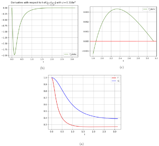
Figure 1: The absolute value function is not always monotone. In (a) we have the plot of $\left\lvert z/(1-z/(1-z)^{2})\right\rvert$ in red color, corresponding to $S_{3}$ as given in (4), where $z{\color[rgb]{1,0,0}\mathop{\mbox{\rm:=}}}\beta e^{it}$, and $\beta\sim 0.318$ is the point where the function takes the value one. The plot in blue color shows the corresponding majorizing function. (b) Shows the derivative with respect to $t$ of the absolute value in $[0,\pi]$ and (c) shows the same graph zoomed in to highlight an additional root of the derivative besides $0$ and $\pi$.

We next need to show that for the points on the circle $\beta(G)e^{i\theta}$ that are outside the disc $D(\beta(G),r_{G}/4)$, there is a disc centered around each of the points such that the value $\left\lvert f_{u}(z)\right\rvert$ is smaller than one on these discs. The following result makes this precise:

Lemma 2.2.

If $|w-\beta(G)e^{i\theta}|\leq r_{G}(1-\left\lvert f_{u}(\beta(G)e^{i\theta})\right\rvert)$ then $|f_{u}(w)|<1$. In other words, there is no root of $I(G,z)$ in the disc $D(\beta(G)e^{i\theta},r_{G}(1-\left\lvert f_{u}(\beta(G)e^{i\theta})\right\rvert))$, for $\theta>0$.

Note that the radius of the disc goes to zero as $\theta$ approaches zero, but this case is already handled in Theorem 2.1. In order to make the bound explicit in terms of graph parameters, we need to upper bound $\left\lvert f_{u}(\beta e^{i\theta})\right\rvert$ for $\theta$ sufficiently far away from the origin. Ideally one would expect $\left\lvert f_{u}(\beta e^{i\theta})\right\rvert$ to monotonically decrease in $\theta$ as it varies from $0$ to $\pi$, but this is not the case, as shown in Figure 1 for the function $z/(1-z/(1-z)^{2})$.

Nevertheless, this is not far away from the truth, since as the depth of $f_{u}(z)$ increases it concentrates around the origin and drops sharply as $\theta$ increases; we are not able to prove this, but our observation is that it has the properties of a “good kernel” [11]. Instead, we show that there is a natural function that majorizes $\left\lvert f_{u}(z)\right\rvert$ on the boundary of the disc $D(0,re^{i\theta})$, within its domain of holomorphy, and that is also monotonically decreasing with $\theta$.

A majorant function $G_{r}(\theta)$ for a complex valued function $g(re^{i\theta})$ satisfies the following two properties:

1. $G_{r}(0)=g(r)$.

2. For all $\theta$, $|g(re^{i\theta})|\leq G_{r}(\theta)$, that is, the function majorizes $g$ on the circle $re^{i\theta}$.

3. It is a monotone decreasing function, i.e., $G_{r}^{\prime}(\theta)\leq 0$; attains its maximum at the origin, i.e., $G^{\prime}_{r}(0)=0$; and it is symmetric about the $y$-axis, i.e., $G_{r}(\theta)=G_{r}(-\theta)$.

For example, consider the function in the base case $z/(1-z)^{\ell}$. Its absolute value on $re^{i\theta}$ is $r/|1-re^{i\theta}|^{\ell}$, which by a simple calculation turns out to be

$$g_{r}(\theta)=\frac{r}{(1-2r\cos\theta+r^{2})^{\ell/2}}.$$

In this case it is easier to argue monotonicity because the derivative with respect to $\theta$ is

$$\frac{-\ell r^{2}\sin\theta}{(1-2r\cos\theta+r^{2})^{(\ell+2)/2}},$$

which is negative for $\theta\in(0,\pi)$. However, we use a simpler majorant function that upper bounds the absolute value in the base case and behaves similarly. Based on the observation that $\left\lvert 1-re^{i\theta}\right\rvert\geq 1-r\cos\theta$, one such function is

$$g_{r}(\theta){\color[rgb]{1,0,0}\mathop{\mbox{\rm:=}}}\frac{r}{(1-r\cos\theta)^{\ell}}.$$ (8)

For $r\leq\beta(G-u)$, consider the function

$$f_{u}(re^{i\theta})=\frac{re^{i\theta}}{(1-re^{i\theta})^{\ell}\prod_{j}(1-g_{j}(re^{i\theta}))},$$

where $j$ varies over some fixed index, and $\ell\geq 0$. A majorant function $F_{u,r}(\theta)$ for $|f_{u}(re^{i\theta})|$ is obtained recursively from the majorant functions $G_{j,r}(\theta)$ for $\left\lvert g_{j}(re^{i\theta})\right\rvert$, respectively, as follows:

$$F_{u,r}(\theta){\color[rgb]{1,0,0}\mathop{\mbox{\rm:=}}}\frac{r}{(1-r\cos\theta)^{\ell}\prod_{j}(1-G_{j,r}(\theta))}.$$ (9)

The reason we treat powers of $(1-re^{i\theta})$ separately is because if we take the absolute value inside, as we will immanently do for the $g_{j}$’s, we will get a constant function $r$. So, in principle, we assume that the $g_{j}$’s have depth more than one.

Let us verify that $F_{u,r}(\theta)$ satisfies all the properties of a majorant function. Firstly,

$$F_{u,r}(0)=\frac{r}{(1-r)^{k}\prod_{j}(1-G_{j,r}(0))}.$$

But as $G_{j,r}(0)=g_{j}(r)$ and the latter is positive it follows that

$$F_{u,r}(0)=\frac{r}{(1-r)^{k}\prod_{j}|1-g_{j}(r)|}=f_{u}(r).$$

Secondly

$$|f_{u}(re^{i\theta})|\leq\frac{r}{|1-re^{i\theta}|^{k}\prod_{j}(1-\left\lvert g_{j}(re^{i\theta})\right\rvert)}\leq\frac{r}{(1-r\cos\theta)^{k}\prod_{j}(1-G_{j,r}(\theta))}=F_{u,r}(\theta)$$

and thirdly, taking the logarithmic derivative with respect to $\theta$ of $F_{u,r}(\theta)$ we obtain

$$\frac{F_{u,r}^{\prime}(\theta)}{F_{u,r}(\theta)}=-\frac{kr\sin\theta}{(1-r\cos\theta)}+\sum_{j}\frac{G^{\prime}_{j,r}(\theta)}{(1-G_{j,r}(\theta))}.$$ (10)

Therefore, the derivative is non-positive since by induction $G^{\prime}_{j,r}(\theta)\leq 0$ and $F_{u,r}(\theta)>0$; moreover, it also vanishes at $\theta=0$, hence, the maximum value is attained at the origin which is equal to $f_{u}(r)\leq 1$, for $r\leq\beta(G)$; the symmetric nature also follows by applying induction to (9).

The majorant function will be used in Lemma 2.2 instead of $\left\lvert f_{u}(\beta e^{i\theta})\right\rvert$. However, we still need a more explicit upper bound on $F_{u,r}(\theta)$. The monotone nature of the function comes to rescue, since locally around the origin we will show that the function is upper bounded by an inverted parabola, that is, $F_{u,r}(\theta)\leq F_{u,r}(0)-c\theta^{2}$ for $\theta\leq\theta_{G}$ and some constant $c$ dependent on graph parameters. Therefore, the upper bound at $\theta_{G}$ holds for all $F_{u,r}(\theta)$, for $\theta>\theta_{G}$. Substituting this upper bound at $\theta_{G}$ in Lemma 2.2 then gives us the desired explicit disc around every point $\beta e^{i\theta}$ that is devoid of roots. In order to derive this local upper bound, we need to derive an upper bound on a variant of the gamma-function for $F_{u,r}(\theta)$. This is done inductively. Define $F_{u}(\theta){\color[rgb]{1,0,0}\mathop{\mbox{\rm:=}}}F_{u,\beta(G)}(\theta)$, that is, $F_{u,r}(\theta)$ with $r=\beta(G)$, and $G_{j}(\theta){\color[rgb]{1,0,0}\mathop{\mbox{\rm:=}}}G_{j,\beta(G)}(\theta)$. Then from (9) it follows that

$$F_{u}(\theta)=\frac{\beta(G)}{(1-\beta(G)\cos\theta)^{\ell}\prod_{j=1}^{d(u)-\ell}(1-G_{j}(\theta))}.$$ (11)

In particular, we show the following result:

Lemma 2.3.

For $F_{u}(\theta)$ defined as in (11), and

$$\Gamma{\color[rgb]{1,0,0}\mathop{\mbox{\rm:=}}}\max_{j=1}^{d}\sup_{m\geq 0}\left\lvert\frac{G_{j}^{(m+1)}(0)}{(m+1)!}\right\rvert^{1/(m+1)}$$

we have

$$\sup_{k\geq 0}\left\lvert\frac{F_{u}^{(k)}(0)}{k!}\right\rvert^{1/k}\leq\frac{2d\Gamma}{\beta(G)}.$$

As a consequence, we have

Lemma 2.4.

If $\theta\leq(\beta(G)/2d)^{2\Delta}$, where $d$ is the maximum degree of $G$, and $\Delta$ is the depth of $F_{u}(\theta)$, then

$$F_{u}(\theta)\leq 1-\frac{(\beta(G)\theta)^{2}}{4}.$$

To express the bound only in terms of $d$, we can use Shearer’s bound $\lambda_{S}(d)$ instead of $\beta(G)$.

Substituting this in Lemma 2.2, we obtain

Corollary 2.5.

Define

$$\theta_{G}{\color[rgb]{1,0,0}\mathop{\mbox{\rm:=}}}\left({\frac{\beta(G)}{4n}}\right)^{\text{dia}(G)}.$$ (12)

Then for all $\theta\geq\theta_{G}$ there is no root of $I(G,z)$ in the disc $D(\beta(G)e^{i\theta},r_{G}(\beta(G)\theta)^{2}/4)$,

Finally, combining this result with Theorem 2.1 gives us Theorem 1.1 as desired.

In the next sections, we develop the proofs and details of the results above.

3 Univalence of $I(G,z)$ around $\beta(G)$

Throughout this section, we use $\beta{\color[rgb]{1,0,0}\mathop{\mbox{\rm:=}}}\beta(G)$, and $v\in V$ as a representative vertex. The function $f_{v}(z)$ given in (3) can also be expressed as

$$f_{v}(z)=\frac{zI(G\setminus N[v],z)}{I(G\setminus v,z)}=1-\frac{I(G,z)}{I(G\setminus v,z)}.$$ (13)

Then $f_{v}(\beta)=1$, $f_{v}(0)=0$, and $f^{\prime}_{v}(0)=1$. The next result gives a lower bound on the growth of $f_{v}$ in the vicinity of $\beta_{G}$.

Lemma 3.1.

At the smallest root $\beta(G)$ of $I(G,z)$, we have $f^{\prime}_{v}(\beta_{G})>1/\beta_{G}$.

Proof.

Taking the derivative on both sides of (13), considering the second formulation, we get that

$$f_{v}^{\prime}(z)=-\left({\frac{I(G,z)}{I(G\setminus v,z)}}\right)^{\prime}=-\frac{I^{\prime}(G,z)}{I(G\setminus v,z)}+\frac{I(G,z)I^{\prime}(G\setminus v,z)}{I(G\setminus v,z)^{2}}.$$

Since $\beta$ is a root of $I(G)$, we get

$$f_{v}^{\prime}(\beta)=-\frac{I^{\prime}(G,\beta)}{I(G\setminus v,\beta)}.$$

Substituting (29) for the derivative, we further obtain that

$$f_{v}^{\prime}(\beta) =\sum_{u\in V}\frac{I(G-N[u],\beta)}{I(G-v,\beta)}$$ (14)

$$=\frac{I(G-N[v],\beta)}{I(G-v,\beta)}+\sum_{u\in V,u\neq v}\frac{I(G-N[u],\beta)}{I(G-v,\beta)}$$

$$=\frac{1}{\beta}+\sum_{u\in V,u\neq v}\frac{I(G-N[u],\beta)}{I(G-v,\beta)},$$

where the last step follows from the definition of $\beta$. Now observe that the graphs $G\setminus N[u]$, for $u\in V\setminus\left\{v\right\}$ and $G\setminus v$ are all subgraphs of $G$. Therefore, from Proposition A.1 we know that their smallest root is larger than $\beta$ and hence the corresponding independence polynomials evaluated at $\beta$ are all positive. This means that the terms in the summation above are all positive, which gives us the desired lower bound on $f^{\prime}_{v}(\beta)$. ∎

∎

We also have a corresponding upper bound on $f^{\prime}_{v}(\beta)$.

Lemma 3.2.

For all $v\in V$, $f^{\prime}_{v}(\beta)\leq\frac{n}{\beta^{\text{dia}(G)}}$, where $\text{dia}(G)$ is the diameter of $G$.

Proof.

Let the vertex set of the graph $G$ be $V={v,v_{1},\ldots,v_{n-1}}$. Again consider (14). We start with a lower bound on the denominator $I(G-v,\beta)$ as follows. We know that $I(G-v,\beta)=\beta I(G-N[v],\beta)$. Let $G_{v}=G-N[v]+v_{1}$ where $v_{1}\in N[v]$, and $\beta_{v}$ be the smallest root of $I(G_{v},z)$. Now $I(G,z)$ is continuously decreasing on the real line starting from the origin down to its smallest root. At the origin we have $I^{\prime}(G,0)=\left\lvert V(G)\right\rvert$. Since $G_{v}$ is a subgraph of $G$, we have $\beta_{v}>\beta$. Therefore,

$$I(G-v,\beta)=\beta I(G-N[v],\beta)=\beta I(G_{v}-v_{1},\beta)\geq\beta I(G_{v}-v_{1},\beta_{v}).$$

Repeating the above argument for vertex $v_{1}$ and so on we obtain $I(G-v,\beta)\geq\beta^{k}$, where $k$ is the maximum distance of any vertex from the vertex $v$. Since the diameter $dia(G)$ of the graph is the longest shortest path in the graph and $\beta<1$ we have

$$I(G-v,\beta)\geq\beta^{\text{dia}(G)}.$$ (15)

Note that $I(G-N[u],\beta)<1$ for all $u\in V$. Substituting these two bounds in (14) we get

$$f^{\prime}_{v}(\beta)\leq\frac{1}{\beta}+\frac{n-1}{\beta^{\text{dia}(G)}}=\frac{\beta^{\text{dia}(G)-1}+n-1}{\beta^{\text{dia}(G)}}\leq\frac{n}{\beta^{\text{dia}(G)}},$$

since $\beta\leq 1$, $\beta^{\text{dia}(G)}\leq 1$. ∎

∎

We next derive an upper bound on higher-order derivatives of $I(G,z)$, which will be useful later.

Lemma 3.3.

Let $\beta$ be the smallest root of $I(G,z)$, then for all $0\leq k\leq n$ we have $\left\lvert I^{(k)}(G,\beta)\right\rvert\leq{n\choose k}\leq n^{k}$. More generally, if $H$ is a subgraph of $G$, then $I^{(k)}(H,\beta)\leq{|H|\choose k}\leq|H|^{k}$.

Proof.

For a general $k$, we have

$$I^{(k)}(G,z)=(-1)^{k}\sum_{\begin{subarray}{c}u_{1}\in V,u_{2}\in G-N[u_{1}],\ldots,\\ u_{k}\in G-{\cup_{j=1}^{k-1}}N[u_{j}]\end{subarray}}I(G-N[u_{1}]-N[u_{2}]-\cdots N[u_{k}],z).$$

Since the graph $G-N[u_{1}]-N[u_{2}]-\cdots N[u_{k}]$ is a subgraph of $G$, its evaluation at $\beta$ is smaller than one. The number of distinct choices of $u_{1},\ldots,u_{k}$ are at most ${n\choose k}$, which completes the proof. ∎

∎

Using the bounds above, we derive an upper bound on $\gamma_{I^{\prime}(G,z)}$ (see (32)), the standard gamma-function for the derivative $I^{\prime}(G,z)$ at $\beta$. We start with deriving a lower bound on $I^{\prime}(G,\beta)$: Since

$$I^{\prime}(G,\beta)=-\sum_{u\in V}I(G-N[u],\beta)$$

and each $I(G-N[u],\beta)$ has the same sign and by (15) is at least $\beta^{\text{dia}(G)}$, we obtain

$$\left\lvert I^{\prime}(G,\beta)\right\rvert\geq n\beta^{\text{dia}(G)}.$$ (16)

It is not hard to see from the bound in Lemma 3.3 above and (16) that

$$\gamma=\gamma_{I^{\prime}(G,z)}(\beta){\color[rgb]{1,0,0}\mathop{\mbox{\rm:=}}}\max_{k=1,\ldots,n}\left\lvert\frac{I^{(k+1)}(G,\beta)}{k!I^{\prime}(G,\beta)}\right\rvert^{1/k}\leq\max_{k=1,\ldots,n}\left\lvert\frac{n^{k+1}}{k!n\beta^{\text{dia}(G)}}\right\rvert^{1/k}\leq\frac{n}{\beta^{\text{dia}(G)}}.$$ (17)

In order to apply Proposition A.2 to $I(G,z)$ centered at $\beta$, we first need to derive an upper bound on $\left\lvert I^{\prime}(G,z)\right\rvert$ in a neighborhood of $\beta$. Consider the Taylor series expansion of the derivative around $\beta$

$$I^{\prime}(G,z)=\sum_{k\geq 0}\frac{I^{(k+1)}(G,\beta)}{k!}(z-\beta)^{k}.$$

Taking absolute values and pulling out the constant term we get

$$\left\lvert I^{\prime}(G,z)\right\rvert\leq\left\lvert I^{\prime}(G,\beta)\right\rvert\sum_{k\geq 0}\left\lvert\frac{I^{(k+1)}(G,\beta)}{k!I^{\prime}(G,\beta)}\right\rvert|z-\beta|^{k}.$$

Substituting the upper bound from (17) in the right-side, we obtain that for $z\in D(\beta,r)$

$$\left\lvert I^{\prime}(G,z)\right\rvert\leq\left\lvert I^{\prime}(G,\beta)\right\rvert\sum_{k\geq 0}\gamma^{k}r^{k}=\frac{\left\lvert I^{\prime}(G,\beta)\right\rvert}{(1-r\gamma)},$$

as long as $r\gamma<1$. By (7), we know that, $r(G)\gamma\leq 1/2$. Therefore, for all $z\in D(\beta,r_{G})$, $\left\lvert I^{\prime}(G,z)\right\rvert\leq 2\left\lvert I^{\prime}(G,\beta)\right\rvert$. Substituting this upper bound, along with the definition of $r(G)$, in Proposition A.2 applied to $I(G,z)$ at $\beta$, we get Theorem 2.1.

4 Gap around every point on the circle with radius $\beta(G)$

In this section, we prove Lemma 2.2, that is, we show that the gap to unity for every $\theta>\theta_{G}$ is governed by the gap of $f_{u}(re^{i\theta})$ to $f_{u}(r)$ and a constant that depends on $r$. We will do the argument only for $r=\beta(G)$. For this purpose, we first need an upper bound on $\left\lvert f^{(k)}_{u}(\beta(G))\right\rvert$. Again, for convenience, let $\beta{\color[rgb]{1,0,0}\mathop{\mbox{\rm:=}}}\beta(G)$.

The $k$th derivative, up to sign, will have the form

$$\left({\frac{I(G,z)}{I(G-u,z)}}\right)^{(k)}=\sum_{j=\max\left\{0,k-n\right\}}^{k}{k\choose j}I(G,z)^{(k-j)}\left({\frac{1}{I(G-u,z)}}\right)^{(j)}.$$ (18)

Applying Arbogast’s formula (33) we obtain

$$\left({\frac{1}{I(G-u,z)}}\right)^{(j)}=\sum_{i_{1},\ldots,i_{j}}\frac{(-1)^{i_{1}+\cdots+i_{j}}}{I(G-u,z)^{1+i_{1}+\cdots+i_{j}}}\frac{j!(i_{1}+\cdots+i_{j})!}{i_{1}!\ldots i_{j}!}\prod_{m=1}^{j}\left({\frac{I^{(m)}(G-u,z)}{m!}}\right)^{i_{m}}$$ (19)

where the sum is over all indices $i_{1},\ldots,i_{j}$ such that

$$i_{1}+2i_{2}+3i_{3}+\cdots+ji_{j}=j$$ (20)

Substituting $z=\beta$ in (18), the term corresponding to $j=k$ disappears in the sum. Plugging the upper bound on the derivatives from Lemma 3.3 in (19) above we get that

$$\frac{\left\lvert f_{u}(\beta)^{(k)}\right\rvert}{k!}\leq\sum_{j=0}^{k-1}\frac{1}{j!(k-j)!}n^{(k-j)}\cdot\sum_{i_{1},\ldots,i_{j}}\frac{1}{I(G-u,\beta)^{1+i_{1}+\cdots+i_{j}}}\frac{j!(i_{1}+\cdots+i_{j})!}{i_{1}!\ldots i_{j}!}\prod_{m=1}^{j}\left({\frac{n^{m}}{m!}}\right)^{i_{m}}.$$

From (36), we obtain that $n^{\sum_{m}mi_{m}}=n^{j}$. Moreover, as $I(G-u,\beta)<1$, we can upper bound its exponent by $k$ as well to get

$$\frac{\left\lvert f_{u}(\beta)^{(k)}\right\rvert}{k!}\leq\left({\frac{n}{I(G-u,\beta)}}\right)^{k}\;\sum_{j=0}^{k-1}\frac{1}{j!(k-j)!}\sum_{i_{1},\ldots,i_{j}}\frac{j!(i_{1}+\cdots+i_{j})!}{i_{1}!\ldots i_{j}!}\prod_{m=1}^{j}\left({\frac{1}{m!}}\right)^{i_{m}}.$$

Using (35) the summation over the indices $i_{1},\ldots,i_{j}$ can be expressed as

$$\frac{\left\lvert f_{u}(\beta)^{(k)}\right\rvert}{k!}\leq\left({\frac{n}{I(G-u,\beta)}}\right)^{k}\;\sum_{j=0}^{k-1}\frac{1}{j!(k-j)!}\sum_{t=0}^{j}t!B_{j,t}(1,\ldots,1),$$

The last summation over $t$ is the ordered Bell number, $\widetilde{B}_{j}$ (see Section A), which gives us

$$\frac{\left\lvert f_{u}(\beta)^{(k)}\right\rvert}{k!}\leq\left({\frac{n}{I(G-u,\beta)}}\right)^{k}\;\sum_{j=0}^{k-1}\frac{\widetilde{B}_{j}}{j!(k-j)!}.$$

Furthermore, applying the upper bound from (38) we derive that

$$\frac{\left\lvert f_{u}(\beta)^{(k)}\right\rvert}{k!}\leq\left({\frac{n}{I(G-u,\beta)}}\right)^{k}\;\sum_{j=0}^{k-1}\frac{2^{j}}{(k-j)!}.$$

Notice that the summation

$$\sum_{j=0}^{k-1}\frac{2^{j}}{(k-j)!}=2^{k}\sum_{j=1}^{k}\frac{1}{j!2^{j}}<2^{k}\sum_{j=1}^{\infty}\frac{1}{j!2^{j}}=2^{k}(e^{1/2}-1)\leq 2^{k}.$$

Therefore, we finally obtain that

$$\frac{\left\lvert f_{u}(\beta)^{(k)}\right\rvert}{k!}\leq\left({\frac{2n}{I(G-u,\beta)}}\right)^{k}.$$

As a consequence, we get that

$$\gamma_{f_{u}}(\beta)\leq\frac{2n}{I(G-u,\beta)}\leq\frac{2n}{\beta^{\text{dia}(G)}}=\frac{1}{r_{G}}.$$ (21)

From this bound, we can derive the following estimate, an alternate proof of Theorem 2.1:

Lemma 4.1.

For all $z\in D(0,\beta+r_{G}/2)$, $\left\lvert f_{u}(z)\right\rvert\leq 2$.

Proof.

A straightforward application of the triangle inequality to the Taylor series of $f_{u}$ around $\beta$ yields

$$\left\lvert f_{u}(z)\right\rvert\leq f_{u}(\beta)\sum_{k\geq 0}(r\gamma_{f_{u}}(\beta))^{k}=\frac{f_{u}(\beta)}{1-r\gamma_{f_{u}}(\beta)}.$$

Since $r\leq r_{G}/2$ it follows that $r\gamma_{f_{u}}(\beta)\leq 2$, whence the upper bound on $|f_{u}(z)|$ in $D(\beta,r_{G}/2)$. Because of the maximum modulus principle, the upper bound holds on the whole disc.

∎

∎

Let $w$ be a point in the vicinity of $\beta(G)e^{i\theta}$. Then taking the Taylor expansion around $\beta(G)e^{i\theta}$, we get the following upper bound:

$$|f_{u}(w)|\leq\left\lvert f_{u}(\beta e^{i\theta})\right\rvert+\sum_{k\geq 1}\frac{|f^{(k)}_{u}(\beta e^{i\theta})|}{k!}|w-\beta e^{i\theta}|^{k}.$$

Since $f_{u}$ is holomorphic with positive coefficients around the origin, from the strong maximum modulus principle, the maximum of $|f^{(k)}_{u}(\beta e^{i\theta})|$ for all $\theta$ is attained at the origin. Now, using the upper bound for $r=\beta$ from (21), we obtain that

$$\left\lvert f_{u}(w)\right\rvert<\left\lvert f_{u}(\beta e^{i\theta})\right\rvert+\sum_{k\geq 1}{\left(\frac{|w-\beta e^{i\theta}|}{r_{G}}\right)}^{k}.$$

Define $r{\color[rgb]{1,0,0}\mathop{\mbox{\rm:=}}}|w-\beta e^{i\theta}|/r_{G}$. If $r<1$ then using the formula for a geometric series we have

$$\left\lvert f_{u}(w)\right\rvert<\left\lvert f_{u}(\beta e^{i\theta})\right\rvert+\frac{r}{1-r}.$$

Therefore, as long as

$$\frac{r}{1-r}\leq 1-\left\lvert f_{u}(\beta e^{i\theta})\right\rvert$$

we have $|f_{u}(w)|<1$, or equivalently, if

$$|w-\beta e^{i\theta}|\leq r_{G}\left({\frac{1-\left\lvert f_{u}(\beta e^{i\theta})\right\rvert}{2-\left\lvert f_{u}(\beta e^{i\theta})\right\rvert}}\right)$$

the function cannot take the value one in the vicinity of $\beta e^{i\theta}$. The denominator can be simplified to one since the maximum value of $\left\lvert f_{u}(\beta e^{i\theta})\right\rvert$ is one at the origin. This completes the proof of the following Lemma 2.2.

5 Upper bound on the Majorant Function near the origin

In this section, we give the proofs of Lemma 2.3 and Lemma 2.4. We again use the shorthand $\beta{\color[rgb]{1,0,0}\mathop{\mbox{\rm:=}}}\beta(G)$. The idea is to consider the Taylor series expansion of $F_{u,r}(\theta)$ around the origin. More precisely, we have

$$F_{u,r}(\theta)=F_{u,r}(0)+F_{u,r}^{\prime}(0)\theta+\sum_{k\geq 2}\frac{F_{u,r}^{(k)}(0)}{k!}\theta^{k}.$$

Since the first derivative vanishes, we have

$$F_{u,r}(\theta)=F_{u,r}(0)+\sum_{k\geq 2}\frac{F_{u,r}^{(k)}(0)}{k!}\theta^{k}.$$

In fact, all the odd derivatives vanish and, the second derivative is negative. We first verify the latter condition. From (10) it follows that

$$F_{u,r}^{(2)}(\theta)=F_{u,r}^{\prime}(\theta)\sum_{j}\frac{G^{\prime}_{j,r}(\theta)}{(1-G_{j,r}(\theta))}+F_{u,r}(\theta)\sum_{j}\left({\frac{G^{(2)}_{j,r}(\theta)}{(1-G_{j,r}(\theta))}+\frac{(G^{\prime}_{j,r}(\theta))^{2}}{(1-G_{j,r}(\theta))^{2}}}\right).$$ (22)

Now inductively, the second derivatives $G_{j,r}^{(2)}(0)$ are negative (the base case from (8) is $-r^{2}/(1-r)^{2}$), all the other terms vanish, which yield us that $F_{u,r}^{(2)}(\theta)(0)<0$ as desired. This means that locally near the origin $F_{u,r}(\theta)\sim F_{u,r}(0)-c\theta^{2}$. We will next show that for $\theta$ sufficiently small, half of the second term will dominate the remaining summation in absolute value, and so $F_{u,r}(\theta)\leq F_{u,r}(0)-F_{u,r}^{(2)}(0)\theta^{2}/4$ for $\theta\leq\theta_{G}$. For this purpose we need an upper bound on the absolute values of the $k$th derivatives of $F_{u,r}$ at the origin with $r=\beta$, which will be used to derive an upper bound on the $\gamma$-function for $F_{u,r}$. The upper bound will be derived inductively.

Let us begin with recalling some definitions: From (11) we have

$$F_{u}(\theta)=\frac{\beta}{\prod_{j=1}^{d(u)}(1-G_{j}(\theta))},$$

where we have simplified the denominator to subsume the functions $\beta\cos\theta$ in the product by appropriate indexing, and $G_{j}(\theta){\color[rgb]{1,0,0}\mathop{\mbox{\rm:=}}}G_{j,\beta}(\theta)$. We next derive a formula for the $k$th derivative of $F_{u}(\theta)$.

It can be verified that for $k\geq 1$,

$$F_{u}^{(k)}(\theta)=\sum_{\ell=0}^{k-1}{k-1\choose\ell}F_{u}^{(k-1-\ell)}(\theta)\sum_{j}-(\ln(1-G_{j}(\theta)))^{(\ell+1)}.$$ (23)

Using Arbogast’s formula, (33), for the functions $\ln(1-G_{j}(\theta))$, along with (41), we further get that

$$F_{u}^{(k)}(\theta)=\sum_{\ell=0}^{k-1}{k-1\choose\ell}F_{u}^{(k-1-\ell)}(\theta)\sum_{j}\sum_{i_{0},\ldots,i_{\ell}}\frac{(\ell+1)!}{i_{0}!\ldots i_{\ell}!}\frac{(i_{0}+\cdots+i_{\ell})!}{(1-G_{j}(\theta))^{\sum_{m=0}^{\ell}i_{m}}}\prod_{m=0}^{\ell}\left({\frac{G_{j}^{(m+1)}(\theta)}{(m+1)!}}\right)^{i_{m}},$$

where $i_{0},\ldots,i_{\ell}$ is an $(\ell+1)$-tuple of non-negative integers satisfying the equation

$$i_{0}+2i_{1}+\cdots+(\ell+1)i_{\ell}=\ell+1.$$ (24)

At this stage, we can inductively argue that if $k$ is odd then the derivative at the origin vanishes; this is because one of the indices $m$ will be odd and by induction $G_{j}^{(m+1)}(0)$ vanishes. Dividing both sides by $k!$, simplifying the binomial ${k-1\choose\ell}$ term, and substituting $\theta=0$ we obtain that

$$\frac{F_{u}^{(k)}(0)}{k!}=\sum_{\ell=0}^{k-1}\frac{F_{u}^{(k-1-\ell)}(0)}{k(k-1-\ell)!\ell!}\sum_{j}\sum_{i_{0},\ldots,i_{\ell}}\frac{(\ell+1)!}{i_{0}!\ldots i_{\ell}!}\frac{(i_{0}+\cdots+i_{\ell})!}{(1-G_{j}(0))^{\sum_{m=0}^{\ell}i_{m}}}\prod_{m=0}^{\ell}\left({\frac{G_{j}^{(m+1)}(0)}{(m+1)!}}\right)^{i_{m}},$$ (25)

Define

$$\Gamma{\color[rgb]{1,0,0}\mathop{\mbox{\rm:=}}}\max_{j=1}^{d}\sup_{m\geq 0}\left({\frac{\left\lvert G_{j}^{(m+1)}(0)\right\rvert}{(m+1)!}}\right)^{1/(m+1)},$$ (26)

which implies that

$$\frac{\left\lvert G_{j}^{(m+1)}(0)\right\rvert}{(m+1)!}\leq\Gamma^{m+1}.$$

Furthermore, we inductively assume that

$$\max_{j=0}^{k-1}\left({\frac{\left\lvert F_{u}^{(j)}(0)\right\rvert}{j!}}\right)^{1/j}\leq\frac{2d\Gamma}{\beta}.$$

Since $F_{u}(0)=1$, we also know that $\prod_{j}(1-G_{j}(0))=\beta$, which implies that for all $j$, $(1-G_{j}(0))\geq\beta$. Taking the absolute value, applying the triangle inequality, and substituting these upper and lower bounds in the right-hand side, we get the following

$$\frac{\left\lvert F_{u}^{(k)}(0)\right\rvert}{k!} \leq\sum_{\ell=0}^{k-1}\left({\frac{2d\Gamma}{\beta}}\right)^{(k-1-\ell)}\frac{1}{k\ell!}\sum_{j}\sum_{i_{0},\ldots,i_{\ell}}\frac{(i_{0}+\cdots+i_{\ell})!(\ell+1)!}{i_{0}!\ldots i_{\ell}!}\prod_{m=0}^{\ell}\left({\frac{\Gamma^{(m+1)}}{\beta}}\right)^{i_{m}}$$

From (24), the term $\prod_{m}\Gamma^{i_{m}(m+1)}=\Gamma^{\ell+1}$ and hence

$$\frac{\left\lvert F_{u}^{(k)}(0)\right\rvert}{k!} \leq\Gamma^{k}\sum_{\ell=0}^{k-1}\left({\frac{2d}{\beta}}\right)^{(k-1-\ell)}\frac{(\ell+1)!}{k\ell!}\sum_{j}\sum_{i_{0},\ldots,i_{\ell}}\frac{(i_{0}+\cdots+i_{\ell})!}{i_{0}!\ldots i_{\ell}!}\left({\frac{1}{\beta}}\right)^{\sum_{m}i_{m}}$$

$$=\Gamma^{k}\sum_{\ell=0}^{k-1}\left({\frac{2d}{\beta}}\right)^{(k-1-\ell)}\frac{(\ell+1)}{k}\sum_{j}\sum_{i_{0},\ldots,i_{\ell}}\frac{(i_{0}+\cdots+i_{\ell})!}{i_{0}!\ldots i_{\ell}!}\prod_{m=0}^{\ell}\left({\frac{1}{\beta}}\right)^{\sum_{m}i_{m}}.$$

The summation term over $j$ is independent of it, so we can upper bound the summation by the degree $d$. Furthermore, if we define $t=i_{0}+\cdots+i_{\ell}$, for a fixed $t$, then the right-hand side further simplifies to

$$\frac{\left\lvert F_{u}^{(k)}(0)\right\rvert}{k!} \leq d\Gamma^{k}\sum_{\ell=0}^{k-1}\left({\frac{2d}{\beta}}\right)^{(k-1-\ell)}\frac{(\ell+1)}{k}\sum_{t=1}^{\ell+1}\frac{1}{\beta^{t}}\sum_{\begin{subarray}{c}i_{0},\ldots,i_{\ell}\\ i_{0}+\cdots+i_{\ell}=t\end{subarray}}\frac{t!}{i_{0}!\ldots i_{\ell}!}$$

$$\leq d\Gamma^{k}\sum_{\ell=0}^{k-1}\left({\frac{2d}{\beta}}\right)^{(k-1-\ell)}\frac{(\ell+1)}{k}\sum_{t=1}^{\ell+1}\frac{1}{\beta^{t}}{\ell+1\choose t-1},$$

where the last step follows from (39). Since $\beta\leq 1$, we can use $\beta^{-(\ell+1)}$ instead of $\beta^{-t}$ to get

$$\frac{\left\lvert F_{u}^{(k)}(0)\right\rvert}{k!} \leq d\left({\frac{\Gamma}{\beta}}\right)^{k}\sum_{\ell=0}^{k-1}\left({2d}\right)^{(k-1-\ell)}\frac{(\ell+1)}{k}\sum_{t=1}^{\ell+1}{\ell+1\choose t-1}$$

$$\leq d\left({\frac{2\Gamma}{\beta}}\right)^{k}\sum_{\ell=0}^{k-1}\frac{(\ell+1)}{k}d^{(k-1-\ell)},$$

where in the last step we upper bound the summation of the binomials by $2^{\ell+1}$. Since $d\geq 2$, it can be showed that the new summation term is at most $d^{k-1}$, which finally yields us the desired claim in Lemma 2.3.

In the base case $\Gamma$ is the standard gamma-function for the cosine function, which is smaller than $1/\sqrt{2}<1$. Therefore, we get

$$\frac{\left\lvert F_{u}^{(k)}(0)\right\rvert}{k!}^{1/k} \leq\left({\frac{2d}{\beta}}\right)^{\Delta},$$

where $\Delta$ is the depth of $f_{u}(z)$.

In order for half of the second term in the Taylor series expansion of $F_{u}(\theta)$ around the origin to dominate the sum of the remaining terms, we want

$$\left\lvert\frac{F_{u}^{(2)}(0)}{4}\right\rvert\theta^{2}\geq\sum_{\ell\geq 2}\left({\frac{2d}{\beta}}\right)^{2\Delta\ell}\theta^{2\ell}.$$

Assuming

$$\theta^{2}\leq(\beta/2d)^{\Delta}/2,$$ (27)

the above inequality follows if

$$\theta^{2}\leq\frac{\left\lvert F_{u}^{(2)}(0)\right\rvert}{4}\left({\frac{\beta}{2d}}\right)^{\Delta}.$$ (28)

We next derive an explicit lower bound on the second-derivative.

Recall that the first derivatives $F_{u}^{\prime}(0)$ and $G_{j}^{\prime}(0)$ vanish, and that the second derivatives $G_{j}^{(2)}(0)$ are all negative. Therefore, from (22) we obtain that

$$F_{u}^{(2)}(0)=\sum_{j}\frac{G_{j}^{(2)}(0)}{(1-G_{j}(0))}\geq\sum_{j}G_{j}^{(2)}(0).$$

Therefore, $\left\lvert F_{u}^{(2)}(0)\right\rvert\geq d\min\left\lvert G_{j}^{(2)}(0)\right\rvert$. Inductively, we obtain that

$$\left\lvert F_{u}^{(2)}(0)\right\rvert\geq d^{\Delta-1}\beta^{2}/(1-\beta)^{d+1},$$

since the absolute value of the second derivative of the majorant function in the base case is $d\beta^{2}/(1-\beta)^{d+1}$. Substituting this in (28), we get a slightly weaker constraint than (27), namely, $\theta^{2}\leq{\beta^{\Delta+2}}/{4d}$. So, in order to simplify, we combine the two constraints to obtain Lemma 2.4.

In order to combine this lemma with Theorem 2.1, we notice that the disc $D(\beta,r_{G}/2)$ subtends the angle $\arcsin(r_{G}/2\beta)$, which is at least $\beta^{\text{dia}(G)}/(4n)$, at the origin. Take $\theta_{G}$ as a quantity smaller than this bound and the constraint in Lemma 2.4, namely as defined in (12). Since the function $F_{u}(\theta)$ is monotonically decreasing, we know that for all $\theta\geq\theta_{G}$, $F_{u}(\theta)\leq F_{u}(\theta_{G})$. Substituting this in Lemma 2.2, we obtain that for all $\theta\geq\theta_{G}$, the disc

$$D(\beta e^{i\theta},r_{G}(\beta\theta_{G})^{2}/4)$$

is devoid of roots. Since the radius here is smaller than $r_{G}/2$, we combine this with Theorem 2.1 to finally obtain that the disc

$$D\left({0,\beta+\left({\frac{\beta}{n}}\right)^{O(\text{dia}(G))}}\right)$$

contains exactly one root of $I(G,z)$ completing the proof of Theorem 1.1. Note that the depth $\Delta$ is smaller than the diameter $\text{dia}(G)$, which instead is bounded by $n$.

6 Some Explicit Lower Bounds On The Gap

In this section, we derive explicit lower bounds on the gap between the smallest root $\beta(G)$ and the root with the second smallest absolute value of the independence polynomial of some fundamental graph classes. In particular, we give the explicit lower bounds for the Path Graph $(P_{n})$, the Cycle Graph $(C_{n})$ on $n$ vertices and the Complete Bipartite Graph $(K_{n\times n})$ on $2n$ vertices. For convenience, let $\beta{\color[rgb]{1,0,0}\mathop{\mbox{\rm:=}}}\beta(G)$ and $\alpha{\color[rgb]{1,0,0}\mathop{\mbox{\rm:=}}}\alpha(G)$ be the root with the second smallest absolute value of the independence polynomial of graph $G$ in each of the cases.

Path Graph

To describe the independence polynomial $P_{n}(z)$ of the Path Graph we need the Fibonacci polynomials [7]: Let $F_{1}(z){\color[rgb]{1,0,0}\mathop{\mbox{\rm:=}}}1$, $F_{2}(z){\color[rgb]{1,0,0}\mathop{\mbox{\rm:=}}}z$ and recursively define $F_{n+1}(z){\color[rgb]{1,0,0}\mathop{\mbox{\rm:=}}}zF_{n}(z)+F_{n-1}(z)$. From the relation (2) for $P_{n}(z)$ we obtain that $z^{n-1}P_{n}(-1/z^{2})=F_{n+2}(z)$. The roots of $F_{n+2}(z)$ are $2i\cos(k\pi/(n+2))$, $k=1,\ldots,n+1$. Therefore, the roots of $P_{n}(z)$ are $1/(4\cos^{2}(k\pi/(n+2)))$, for $k=1,\ldots,\lfloor\frac{n+1}{2}\rfloor$. Therefore, $\beta=\frac{1}{4\cos^{2}\left(\frac{\pi}{m}\right)}$ and $\alpha=\frac{1}{4\cos^{2}\left(\frac{2\pi}{m}\right)}$, with $m{\color[rgb]{1,0,0}\mathop{\mbox{\rm:=}}}n+2$. Using the Taylor series for the cosine function, for large values of $m$, we get

$$\frac{\cos\left(\frac{\pi}{m}\right)}{\cos\left(\frac{2\pi}{m}\right)}=1+\frac{3\pi^{2}}{2m^{2}}+O(m^{-4}).$$

On squaring, we obtain that

$$\frac{\alpha}{\beta}=\frac{\cos^{2}\left(\frac{\pi}{m}\right)}{\cos^{2}\left(\frac{2\pi}{m}\right)}=1+\frac{3\pi^{2}}{m^{2}}+O(m^{-4})=1+\Omega\left(\frac{1}{n^{2}}\right).$$

Cycle Graph

The independence polynomial $C_{n}(z)$ of the Cycle Graph can be expressed in terms of the Chebyshev polynomial of the first kind $T_{n}(z)$ [9]:

$$C_{n}(z)=2z^{n/2}T_{n}\left({\frac{1}{2\sqrt{z}}}\right).$$

Therefore, its roots are $\frac{1}{4\cos^{2}\left(\frac{(2k+1)\pi}{2n}\right)}$, $k=0,1,\ldots,\lfloor\frac{n-1}{2}\rfloor$. This implies that $\beta=\frac{1}{4\cos^{2}\left(\frac{\pi}{2n}\right)}$ and $\alpha=\frac{1}{4\cos^{2}\left(\frac{3\pi}{2n}\right)}$. An argument similar to the one above implies that asymptotically we have

$$\frac{\alpha}{\beta}=1+\frac{2\pi^{2}}{n^{2}}+\frac{17\pi^{4}}{6n^{4}}+O(n^{-6})=1+\Omega\left({\frac{1}{n^{2}}}\right).$$

Complete Bipartite Graph

The independence polynomial $K_{n\times n}(z)$ of the Complete Bipartite Graph on $2n$ vertices is $K_{n\times n}(z)=2{(1-z)}^{n}-1$. Its roots are $z_{k}=1-2^{-\frac{1}{n}}e^{\frac{i2k\pi}{n}}$, $k=0,1,\ldots,n-1$. Therefore $\beta=1-2^{-\frac{1}{n}}$ and $\alpha=1-re^{i\frac{2\pi}{n}}$, where $r{\color[rgb]{1,0,0}\mathop{\mbox{\rm:=}}}2^{-\frac{1}{n}}$. Since, in this case $\alpha$ is a complex root, we compute ratio of the absolute values of the roots:

$$\frac{\left|\alpha\right|}{\beta}=\frac{\sqrt{1+r^{2}-2r\cos(\frac{2\pi}{n})}}{1-r}=\frac{\sqrt{{(1-r)}^{2}+4r\sin^{2}(\theta/2)}}{1-r}=\sqrt{1+\frac{4r}{({1-r}^{2})}\sin^{2}\left(\theta/2\right)}.$$

Take $b{\color[rgb]{1,0,0}\mathop{\mbox{\rm:=}}}\ln(2)$ then, $r=e^{-b/n}=1-\frac{b}{n}+\frac{b^{2}}{2n^{2}}+O(n^{-3})$ and $\sin(\frac{\pi}{n})=\frac{\pi}{n}-\frac{\pi^{3}}{6n^{3}}+O(n^{-5})$. After substituting these estimates and simplifying we get that for large $n$

$$\frac{\left|\alpha\right|}{\beta} =\sqrt{1+\frac{4\pi^{2}}{b^{2}}+\left(\frac{-\pi^{2}}{3}-\frac{4\pi^{4}}{3b^{2}}\right)\frac{1}{n^{2}}+O(n^{-3})}$$

$$=\sqrt{1+\frac{4\pi^{2}}{b^{2}}}-\frac{\pi^{2}}{6}\frac{1}{n^{2}}+O(n^{-3})$$

$$\approx 9.119-O\left(\frac{1}{n^{2}}\right).$$

7 Concluding Remarks

This paper provides the first quantitative lower bound on the gap between the smallest root of the independence polynomial and the second smallest absolute value. A simple proof for the existence of the gap can be based on the maximum modulus principle. Quantifying the principle for the special function at hand involves studying its local behaviour. To the best of our knowledge, this is the first time a result is provided for separation between roots of the independence polynomial; earlier results always focus on zero-free regions. Our larger hope is to study the algorithmic implications of the ratio of $\beta(G)$ to the second smallest absolute value. Can it be used to design algorithms that are efficient for those graphs where this ratio is large, for example, the graph classes mentioned in Section 6?

Appendix A Basic Results

Throughout this paper $G=(V,E)$ will be assumed to be a simple undirected graph. Let $n$ be the number of vertices in $G$. For every vertex $u\in V$, let $d(u)$ denote its degree, and $d{\color[rgb]{1,0,0}\mathop{\mbox{\rm:=}}}\max_{u}d(u)$, for all $u$; we will assume that $d\geq 2$. Let $\text{dia}(G)$ denote the diameter of $G$, that is the length of the longest path between any pair of vertices in any connected component of $G$. In the subsequent sections, we will need some basic properties of the independence polynomial (see [3, 1] for proofs):

Proposition A.1.

Let $G$ be as above and $I(G,z)$ be its independence polynomial.

1. The derivative $I^{\prime}(G,z)$ satisfies

   $$I^{\prime}(G,z)=-\sum_{u\in V}I(G-N[u],z).$$ (29)

2. If $H$ is a subgraph of $G$ then $\beta(G)\leq\beta(H)$.

3. Shearer [10] showed a lower bound on $\beta(G)$, namely,

   $$\beta(G)\geq\lambda_{S}(d){\color[rgb]{1,0,0}\mathop{\mbox{\rm:=}}}\frac{(d-1)^{d-1}}{d^{d}}.$$ (30)

   Applying the third property with $G$ as the complete graph and $H$ an arbitrary graph with at most $n$ vertices, we also have the following lower bound

   $$\beta(H)\geq\frac{1}{n}.$$ (31)

We will also need variants of Smale’s gamma-function [2]: Given a function $f:{\mathbb{C}}\rightarrow{\mathbb{C}}$ holomorphic at a point $z\in{\mathbb{C}}$, such that $f^{(j)}(z)\neq 0$, define

$$\gamma_{f,j}(z){\color[rgb]{1,0,0}\mathop{\mbox{\rm:=}}}\sup_{k>j}\left\lvert\frac{j!f^{(k)}(z)}{k!f^{(j)}(z)}\right\rvert^{1/(k-j)}.$$ (32)

The standard gamma-function corresponds to $\gamma_{f,0}(z)$, and we will simply use $\gamma_{f}(z)$ to denote that. Intuitively, the function is related to the inverse of the radius of convergence of $f^{(j)}(z)$ at $z$.

We recall Arbogast’s formula (also called the formula of Faà di Bruno) [8] for derivatives of composition of functions: For $N\in{\mathbb{Z}}_{\geq 0}$, the $N$th derivative of

$$(f\circ g)^{(N)}(z)=\sum_{i_{1},\ldots,i_{N}}\frac{N!}{i_{1}!\ldots i_{N}!}f^{(i_{1}+\cdots+i_{N})}(g(z))\prod_{m=1}^{N}\left({\frac{g^{(m)}(z)}{m!}}\right)^{i_{m}},$$ (33)

where the sum is over all tuples of non-negative integers $i_{1},\ldots,i_{N}$ such that

$$i_{1}+2i_{2}+3i_{3}+\cdots+Ni_{N}=N.$$

Given a $K$, we can combine the terms corresponding to $i_{1}+\cdots+i_{N}=K$ and simplify the summation as follows. Since $\sum_{j}ji_{j}=N$ it follows with the additional constraint that $\sum_{j}(j-1)i_{j}=N-K$. This implies that $i_{j}=0$, for $j>N-K+1$, and so we can express (33) as

$$(f\circ g)^{(N)}(z)=\sum_{K=0}^{N}\sum_{i_{1},\ldots,i_{N}}f^{(K)}(g(z))B_{N,K}(g^{\prime}(z),g^{(2)}(z),\ldots,g^{(N-K+1)}(z)),$$ (34)

where $B_{N,K}(x_{1},\ldots,x_{N-K+1})$ are the partial exponential Bell polynomials:

$$B_{N,K}(x_{1},\ldots,x_{N-K+1}){\color[rgb]{1,0,0}\mathop{\mbox{\rm:=}}}\sum_{i_{1},\ldots,i_{N-K+1}}\frac{N!}{i_{1}!\ldots i_{N-K+1}!}\prod_{m=1}^{N-K+1}\left({\frac{x_{m}}{m!}}\right)^{i_{m}},$$ (35)

and $i_{1},\ldots,i_{N-K+1}$ satisfy the following two constraints:

$$\begin{split}i_{1}+2i_{2}+3i_{3}+\cdots+(N-K+1)i_{N-K+1}=N\text{ and }\\ i_{1}+i_{2}+i_{3}+\cdots+i_{N-K+1}=K.\end{split}$$ (36)

Notice that $B_{N,K}(1,\ldots,1)=\genfrac{\{}{\}}{0.0pt}{}{N}{K}$, the Sterling number of second kind, that is number of ways to partition an $N$ element set into $K$ non-empty parts, and hence

$$\sum_{K=0}^{N}K!B_{N,K}(1,\ldots,1)=\widetilde{B}_{N}$$

the ordered Bell number, which satisfy the following recurrence:

$$\widetilde{B}_{N}=\sum_{i=1}^{N-1}{N\choose i}\widetilde{B}_{i}.$$ (37)

From this, we can derive the following claim inductively:

$$\frac{\widetilde{B}_{N}}{N!}\leq\left({\frac{1}{\ln 2}}\right)^{N}.$$ (38)

We will also need the following observation:

$$\sum_{i_{1},\ldots,i_{N-K+1}}\frac{K!}{i_{1}!\ldots i_{N-K+1}!}={N-1\choose K-1}$$ (39)

where the sum is over all tuples $(i_{1},\ldots,i_{N})$ satisfying the conditions in (36). The left-hand side counts all partition of $N$ into $K$ blocks where the ordering of distinct blocks only matter (distinct blocks correspond to different choices of $j$). However, these are precisely the number of compositions of $N$ into $K$ parts, which is the term on the right-hand side.

Besides the above, we need the following observations for $j\geq 0$

$$\left({\frac{1}{x}}\right)^{(j)}=\frac{(-1)^{j}j!}{x^{j+1}}$$ (40)

and

$$\left({\ln x}\right)^{(j)}=\left({\frac{1}{x}}\right)^{(j-1)}=\frac{(-1)^{j-1}(j-1)!}{x^{j}}.$$ (41)

Given $\alpha\in{\mathbb{C}}$ and $r>0$, we will denote by $D(\alpha,r)\subset{\mathbb{C}}$ the open disc centered at $\alpha$ with radius $r$.

In addition to the above, we need the following quantified result on the injectiveness of a function in a neighborhood of a point where the derivative does not vanish [6]:

Proposition A.2.

Let $h:D(\alpha,r)\rightarrow{\mathbb{C}}$ be a holomorphic function such that $h(\alpha)=0$ and $h^{\prime}(\alpha)\neq 0$. Then $h$ is injective on the disc

$$D\left({\alpha,\frac{r|h^{\prime}(\alpha)|}{\sup_{z\in D(\alpha,r)}|h^{\prime}(z)|}}\right).$$

References

- [1] F. Bencs, P. Csikvári, P. Srivastava, and J. Vondrák. On complex roots of the independence polynomial. In N. Bansal and V. Nagarajan, editors, Proceedings of the 2023 Annual ACM-SIAM Symposium on Discrete Algorithms (SODA), pages 675–699, 2023.
- [2] L. Blum, F. Cucker, M. Shub, and S. Smale. Complexity and Real Computation. Springer-Verlag, New York, 1998.
- [3] P. Csikvári. Note on the smallest root of the independence polynomial. Combinatorics, Probability and Computing, 22:1–8, 2012.
- [4] P. Flajolet and R. Sedgewick. Analytic Combinatorics. Cambridge University Press, USA, 1 edition, 2009.
- [5] M. Goldwurm and M. Santini. Clique polynomials have a unique root of smallest modulus. Information Processing Letters, 75(3):127–132, 2000.
- [6] L. A. Harris. On the size of balls covered by analytic transformations. Monatshefte für Mathematik, 83(1):9–23, Mar 1977.
- [7] V. E. H. Jr. and M. Bicknell. Roots of Fibonacci Polynomials. The Fibonacci Quarterly, 11(3):271–274, 1973.
- [8] S. G. Krantz and H. R. Parks. A Primer of Real Analytic Functions. Birkhäuser, 2012.
- [9] V. E. Levit and E. Mandrescu. The independence polynomial of a graph–a survey. In Proceedings of the 1st International Conference on Algebraic Informatics, volume 233254, pages 231–252. Aristotle Univ. Thessaloniki Thessaloniki, 2005.
- [10] J. Shearer. On a problem of Spencer. Combinatorica, 5:241–245, 1985.
- [11] E. M. Stein and R. Shakarchi. Fourier Analysis: An Introduction. Princeton University Press, 2003.