Co-designing a Programmable RISC-V Accelerator for MPC-based Energy and Thermal Management of Many-Core HPC Processors

Abstract

Managing energy and thermal profiles is critical for many-core HPC processors with hundreds of application-class processing elements (PEs). Advanced model predictive control (MPC) delivers state-of-the-art performance but requires solving an online optimization problem over a thousand times per second (1kHz control bandwidth), with computational and memory demands scaling with PE count. Traditional MPC approaches execute the controller on the PEs, but operating system overheads create jitter, and limit control bandwidth. Running MPC on dedicated on-chip controllers enables fast, deterministic control but raises concerns about area and power overhead. In this work, we tackle these challenges by proposing a hardware-software codesign of a lightweight MPC controller, based on an operator splitting quadratic programming solver, and an embedded multi-core RISC-V controller. Key innovations include pruning weak thermal couplings to reduce model memory and ahead-of-time scheduling for efficient parallel execution of sparse triangular systems arising from the optimization problem. The proposed controller achieves sub-millisecond latency when controlling 144 PEs at 500 MHz, delivering 33 lower latency and 7.9 higher energy efficiency than a single-core baseline. Operating within a compact $<$ 1 MiB memory footprint, it consumes as little as 325 mW while occupying less than 1.5% of a typical high performance computing (HPC) processor’s die area.

I Introduction

With the growing computational demands of high performance computing (HPC), processors have evolved into complex heterogeneous systems, integrating general-purpose (GP) and domain-specific (DS) sub-domains to efficiently tackle diverse compute-intensive tasks ranging from artificial intelligence (training and inference) [1], to quantum and molecular simulations [2], and computational biology [3].

HPC processors must deliver high floating-point operations per second ($\mathrm{FLOP}\text{/}\mathrm{s}$), and energy efficiency ($\mathrm{FLOP}\text{/}\mathrm{s}\text{/}\mathrm{W}$), to address growing operational costs and sustainability challenges [4]. Achieving these objectives requires real-time management of the processors’ thermal and power profiles to implement effective thermal and power capping policies and optimize the energy efficiency of the whole computing system. One approach involves advanced cooling strategies, to improve heat dissipation [5, 6]. A complementary approach leverages dynamic thermal and power management techniques, or runtime active control (RAC), to mitigate the negative effects of increased power density in modern technology nodes — including reduced component lifespan, electromigration, and dielectric breakdown — which are often triggered by thermal hotspots and steep thermal gradients during workload execution.

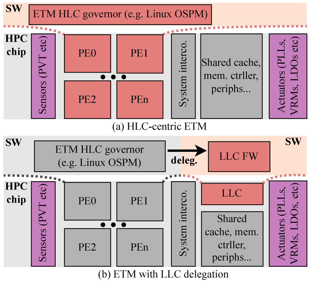
Figure 1: Illustration of HLC (a) and LLC (b) centric paradigms for ETM of HPC chips. Blocks in red indicate the hardware/software entity responsible for low-level interaction with sensors and actuators (in purple) during RAC.

RAC uses process, voltage, and temperature (PVT) data from on-chip sensors and online workload information to choose optimal dynamic voltage and frequency scaling (DVFS) operating points for the chip within imposed power and thermal limits. These settings are applied at runtime to chip actuators like phase locked loops (PLLs) and voltage regulator modules (VRMs) connected to the processing elements (PEs), which are commonly large, out-of-order application-class processors with vector engines. The combination of static and dynamic methods is collectively called the energy and thermal management (ETM) policy of an HPC processor. As shown in Figure 1, the ETM landscape has shifted over the last decade from high-level controller (HLC) centric policies — software routines like the Linux operating system-directed configuration and power management (OSPM) governor running on the same PEs to be controlled — to a delegation-based paradigm, where a hardware low-level controller (LLC) collaborates with the HLC to enforce power and thermal policies [7, 8].

The delegation-based approach brings several benefits to ETM from a real-time scheduling perspective. For example, processor thermal conditions can change so quickly that HLC software policies cannot deal with them in a timely manner [9]. In contrast, LLCs can provide faster and more deterministic response times through (i) low-level and autonomous access to the controlled system, (ii) a streamlined and domain-specific hardware-software stack with fast and deterministic access to hardware sensors and actuators like a lightweight real-time OS (RTOS), and (iii) a microarchitecture tuned to meet real-time constraints. Furthermore, the PEs may be forced to remain active or wake up to perform low-level control functions without other primary tasks. Decoupled LLCs provide an always-on intelligence that is low-power, flexible, timely, and able to act autonomously or in collaboration with the HLC [7]. In its simplest form, a LLC is a low-end single-core microcontroller unit (MCU) with limited compute capabilities. However, continuous advancements in transistor scaling have enabled the integration of more performant, heterogeneous, mid-end embedded LLCs on HPC dies. Examples include ControlPULP [8], which combines a single-core manager domain with a programmable multi-core accelerator (PMCA), and IBM’s on-chip controller [10], which integrates four microcode engines.

On the algorithmic side, established ETM control policies are closed-loop multiple-input multiple-output (MIMO) algorithms ranging from simple hardware-triggered capping without DVFS to classic proportional integral derivative (PID) controllers [10] for reactive setpoint tracking and DVFS enforcement. However, these methods are not sufficiently flexible and powerful to capture and control the dynamic behavior of many-core processors [11, 12]. For this reason, in the last decade, predictive policies such as model predictive control (MPC) algorithms have been investigated as more advanced alternatives beyond reactive RAC [13, 11, 6, 12]. Notably, one of the main challenges of MPC is the high computational cost of solving an optimization problem on every iteration. In ETM applications, this cost grows with the number of controlled PEs, nowadays ranging from under 100 [14, 15] to over 200 [16] on the same die. For such complex systems, the large resulting model heavily impacts the memory footprint and computational work of the underlying optimization algorithm [17].

These factors present challenges and opportunities for implementing predictive ETM policies within the modern delegation-based framework. Challenges arise from an LLC’s limited computational and memory resources, even when enhanced with dedicated accelerators. On the other hand, opportunities emerge from the growing interest in MPC on embedded devices, driving the development of lightweight, optimized, and fast MPC algorithms for resource-constrained MCUs particularly in commodity and miniaturized robotics applications [18, 19].

In this paper, we present a fast, lightweight, hardware-software LLC capable of supporting MPC for online energy and thermal management of HPC processors. We leverage a low-cost RISC-V LLC, which integrates an energy-efficient eight-core PMCA with custom extensions maximizing compute utilization [20]. We base our approach on the state-of-the-art (SoA) operator-splitting quadratic programming (OSQP) solver and the alternating direction method of multipliers (ADMM) solver [21] to minimize memory usage by exploiting the sparsity of the quadratic programming (QP) formulation. We further reduce model complexity by introducing a novel pruning technique that eliminates weak thermal couplings among PEs far apart in the chip. To enhance parallel execution on the LLC’s PMCA, we propose a novel ahead-of-time (AOT) scheduling and code generation algorithm atop OSQP that extracts inherent parallelism from the problem’s sparsity pattern. The proposed optimization framework applies to any QP problem beyond the specific use case of ETM. The hardware and software is released under a permissive license.

In more detail, this work makes the following contributions:

• Design of a model-predictive ETM control policy for many-core HPC processors (Section IV), tailored for online execution on the multi-core embedded RISC-V LLC ControlPULP [8] (Section III). Unlike SoA approaches [11], our MPC model incorporates both power and temperature dynamics. The implementation utilizes OSQP’s native QDLDL direct solver (Section II-C), which solves a sparse triangular linear system solver (SpTRSV) during the forward elimination (FE) and backward substitution (BS) passes. The controller design links hardware-agnostic model in the loop (MIL) optimization with hardware-aware deployment on the LLC through OSQP’s native code generation feature (Section V-B).

• Development of a threshold-based pruning algorithm to optimize the model memory usage. The algorithm removes low-magnitude couplings among PE in the state matrices. This optimization reduces the MPC model complexity from quadratic to linear with respect to the number of PEs, significantly enhancing scalability for centralized control in larger many-core systems (Section IV-D).

• Design of an AOT scheduling algorithm, named parallel sparsity-pattern-leveraging triangular linear system solver (ParSPL), to accelerate QDLDL’s SpTRSV on the multi-core LLC. ParSPL uses AOT partial level scheduling and tiling in the SpTRSV to extract more parallelism from the problem’s sparsity pattern and schedule the execution in advance; this dramatically reduces the synchronization steps among the LLC’s compute cores compared to a naive parallelization by column/row (Section V-D). Furthermore, ParSPL leverages the chosen LLC’s extensions for sparse workloads and floating-point hardware loops [20] to eliminate memory and control overheads and maximize compute utilization (Section V-E).

• Deployment and assessment of the algorithm on the embedded multi-core LLC in cycle-accurate simulations. For one SpTRSV iteration on a large ETM problem controlling 144 PEs, our methodology is 33 faster and 7.9 more energy efficient than vanilla single-core OSQP while fitting in $<$$1\text{\,}\mathrm{MiB}$ of on-chip scratchpad memory (SPM). The controller consumes at most $325\text{\,}\mathrm{mW}$ while occupying under $1.5\text{\,}\mathrm{\char 37\relax}$ of a typical HPC processor die. Our approach consumes minimal power and maximizes energy efficiency, unlike HLC-centric methods that incur high overhead from power-hungry, operating system (OS)-based software stacks for thermal and power capping.

The paper is structured as follows: Section II covers fundamental concepts of QP and its connection to MPC. Section III details the multi-core LLC hardware, including extensions for sparse workloads and memory hierarchy. Section IV introduces the thermal and power model for an HPC processor, the MPC controller architecture, and the threshold-based pruning algorithm, highlighting the application’s demanding memory and computational needs. Section V describes the solver optimization framework, emphasizing numerical precision and the ParSPL approach. Finally, Section VI assesses execution latency, memory footprint, and energy and area efficiency of the optimized solver on the LLC across varying problem sizes.

II Background

In this section, we review the fundamentals of quadratic programming (QP), the operator-splitting quadratic programming (OSQP) solver, and its alternating direction method of multipliers (ADMM)-based solution approach. Finally, we discuss MPC and its formulation as a QP.

II-A Convex quadratic program formulation

Solving a convex QP optimization problem [22] means finding a vector of decision variables $x\in\mathbb{R}^{n}$ that:

$$\textnormal{minimize}\quad(1/2)x^{T}Px+q^{T}x$$ (1)

$$\textnormal{subject to}\quad l\leq Ax\leq u$$

The objective function is defined by a positive semi-definite matrix $P\in\mathbb{R}_{+}^{n}$ and a vector $q\in\mathbb{R}^{n}$; the constraints function is defined by a matrix $A\in\mathbb{R}^{m\times n}$. The constraints $l$ and $u$ belong to a set $\mathcal{C}$ s.t.

$$\mathcal{C}=[l,u]=\{z\in\mathbb{R}^{m}\;|\;l_{i}\leq z_{i}\leq u_{i},i=1,.m\}$$ (2)

If $l_{i}=u_{i}$ for some or all elements in $[u,l]$, the problem is equality-constrained. $n$ and $m$ represent the number of decision variables and constraints, respectively [23].

The size of the problem in Equation 1 is defined by a tuple $(n,m,N_{nnz})$. $N_{nnz}$ is the number of nonzero entries in the objective and constraint matrices $P$ and $A$, respectively:

$$N_{nnz}=nnz(P)+nnz(A);\;P\in\mathbb{R}_{+}^{n},\;A\in\mathbb{R}^{m\times n}$$ (3)

where $nnz(\cdot)$ returns the number of non-zeros (fill-ins) of a matrix.

II-B QP solution: the resurgence of first-order methods

Well-known QP solution methods include gradient, active-set, interior-point, and first-order approaches [23].

Gradient methods iteratively solve unconstrained QP problems and project the solution onto the feasible set, with variants like the fast gradient (FG) being suitable for input-constrained problems [24, 17]. Active-set methods iteratively modify the active set of constraints to converge to the optimal solution, while interior-point methods rely on barrier functions to handle constraints but face scalability issues, making them less practical for embedded platforms [25, 22, 23].

In contrast, first-order methods only use information about the objective function’s first derivative (gradient), are amenable to low-precision number formats, and can be efficiently parallelized [17]. Despite providing low- and medium-accuracy solutions, high-quality control can still be achieved without solving the QP in Equation 1 to full accuracy, particularly for real-time embedded optimization [26, 27]; if high-accuracy is desired, techniques like solution polishing [23] can enhance accuracy and robustness if necessary at the cost of additional computation. For these reasons, these methods have seen renewed interest in recent years.

In this work, we focus on a class of first-order methods called operator splitting. They have been proven effective for problems that need to be solved in real-time under tight sampling periods, e.g., embedded control applications [28]. Decomposition schemes split the problem into two parts: a quadratic optimal control problem and a set of single-period optimization problems. An iteration alternating these two steps then converges to a solution [27].

ADMM is a particular splitting technique that applies the method of augmented Lagrange multipliers. By introducing the splitting variables $\tilde{x}\in\mathbb{R}^{n}$ and $\tilde{z}\in\mathbb{R}^{m}$, the problem in Equation 1 can be rewritten in consensus form [27, 23]:

$$\textnormal{minimize}\quad(1/2)x^{T}Px+q^{T}x+\mathcal{I}_{Ax=z}(\tilde{x},\tilde{z})+\mathcal{I}_{\mathcal{C}}(z)$$ (4)

$$\textnormal{subject to}\quad(\tilde{x},\tilde{z})=(x,z)$$

where $\mathcal{I}_{Ax=z}(\tilde{x},\tilde{z})$ and $\mathcal{I}_{\mathcal{C}}(z)$ are the indicator functions that equal $0$ when $Ax=z$ and $z\in\mathcal{C}$, respectively, or are $+\infty$ otherwise. The $k$ ADMM iteration of Equation 4 is obtained from alternating the minimization of its augmented Lagrangian over $\tilde{x}$ and $\tilde{z}$ as follows:

$$(\tilde{x}^{k+1},\tilde{z}^{k+1})\leftarrow \operatorname{argmin}_{(\tilde{x},\tilde{z}):A\tilde{x}=\tilde{z}}(1/2)\tilde{x}^{T}P\tilde{x}+q^{T}\tilde{x}$$ (5)

$$+(\sigma/2)\lVert\tilde{x}-x^{k}+\sigma^{-1}w^{k}\rVert^{2}_{2}$$

$$+(\rho/2)\lVert\tilde{z}-z^{k}+\rho^{-1}y^{k}\rVert^{2}_{2}$$

$$x^{k+1}\leftarrow\alpha\tilde{x}^{k+1}+(1-\alpha)x^{k}+\sigma^{-1}w^{k}$$ (6)

$$z^{k+1}\leftarrow\Pi\left(\alpha\tilde{z}^{k+1}+(1-\alpha)z^{k}+\rho^{-1}y^{k}\right)$$ (7)

$$y^{k+1}\leftarrow y^{k}+\rho\left(\alpha\tilde{z}^{k+1}+(1-\alpha)z^{k}-z^{k+1}\right)$$ (8)

$x$ and $z$ are the primal variables, $\sigma>0$ and $\rho>0$ are the step-size parameters, $\alpha\in(0,2)$ is the relaxation parameter, and $\Pi=\max(\min(z,u),l)$ is the Euclidean projection onto $\mathcal{C}$ [23, 29]. $y^{k}$ is the dual variable associated with the equality constraint $\tilde{z}=z$. Note that $x$ and $z$ are updated in an alternating fashion. Hence the term alternating direction [21].

II-C The OSQP general-purpose solver

Algorithm 1 OSQP solver

1:given init. vals. $x^{0}$, $z^{0}$, $y^{0}$, params. $\rho>0$, $\sigma>0$, $\alpha\in(0,2)$

2:repeat

3:  $\textnormal{solve}\left[\begin{array}[]{@{}cc@{}}P+\sigma I&A^{T}\\ A&-\rho^{-}1I\end{array}\right]\left[\begin{array}[]{@{}c@{}}\tilde{x}^{k+1}\\ \nu^{k+1}\end{array}\right]=\left[\begin{array}[]{@{}c@{}}\sigma x^{k}-q\\ z^{k}-\rho^{-}1y^{k}\end{array}\right]$

4:  $z^{k+1}\leftarrow z^{k}+\rho^{-1}(\nu^{k+1}-y^{k})$

5:  $x^{k+1}\leftarrow\alpha\tilde{x}^{k+1}+(1-\alpha)x^{k}+\sigma^{-1}w^{k}$

6:  $z^{k+1}\leftarrow\Pi\left(\alpha\tilde{z}^{k+1}+(1-\alpha)z^{k}+\rho^{-1}y^{k}\right)$

7:  $y^{k+1}\leftarrow y^{k}+\rho\left(\alpha\tilde{z}^{k+1}+(1-\alpha)z^{k}-z^{k+1}\right)$

8:until termination criteria or max_iter reached

OSQP is an SoA general-purpose solver for constrained QP problems based on ADMM. The solver pseudocode is shown in Algorithm 1. For a complete overview of how to derive the optimality conditions in 3 and 4 from the $\tilde{x}$ and $\tilde{z}$ updates in Equation 5, refer to [23] and [21], Section 4.2.5. We call the coefficient matrix in 3 of Algorithm 1 the Karush-Kuhn-Tucker (KKT) matrix, and label it $K$. OSQP combines the advantages inherited from first-order operator splitting methods with a streamlined, open-source software package to produce, among other outputs, embedded C code. In the following, we summarize its main features.

II-C1 Precomputation, caching, and sparsity

The default QDLDL direct solver used to solve the linear system in 3 of Algorithm 1 comprises two steps: (i) Cholesky factorization of the KKT matrix $K$ so that $K=LDL^{T}$, where $L$ is a lower triangular matrix and $D$ a diagonal matrix with nonzero diagonal elements, and (ii) lower and upper SpTRSV through FE and BS, respectively. To make the algorithm division-free, thereby reducing the execution time of the QP problem, one can divide all the rows of the triangular matrix $L$ by the diagonal element of that row and move the divider into the $D$ matrix as compensation. Then, the $D^{-1}$ can be stored offline.

To improve memory efficiency, OSQP leverages problem sparsity and allows for offline pre-computation of the coefficient matrix $K$, caching it before ADMM is run online. The matrix $K$ in 3 is block-sparse and quasi-definite. OSQP uses approximate minimum degree (AMD) [30] to compute the $LDL^{T}$ factorization of sparse matrices. AMD reorders the matrix $K$ with a permutation matrix $P$ so that $PKP^{T}=LDL^{T}$, reducing the fill-ins introduced in $L$ during factorization. The factorization of the permuted matrix then comprises two steps: (i) symbolic factorization, where the sparsity pattern for $L$ is computed based only on the nonzero pattern of $K$, and (ii) numerical factorization, which computes the numerical values of $L$. The symbolic and numerical factorizations can be computed only once, then stored and reused if only the vectors $q$, $l$, and $u$ in Equation 1 change for each ADMM iteration, a typical scenario for linear MPC [23] and also this work.

Sections IV-C and V-D detail how these features are leveraged for optimal configuration of the OSQP library and AOT scheduling of the sparse QDLDL solver, respectively.

II-C2 Termination

In each iteration $k$, Algorithm 1 produces the triplet $(x^{k},z^{k},y^{k})$. The problem in Equation 1 is considered solvable if the primal and dual residuals converge to zero:

$$\lim_{k\to\infty}r_{\text{prim}}^{k}=0,\quad\lim_{k\to\infty}r_{\text{dual}}^{k}=0$$

where the primal residual $r_{\text{prim}}=Gx-z$ represents how well the current solution satisfies the problem constraints, and the dual residual $r_{\text{dual}}=Px+q+G^{T}y$ reflects how far the current solution is from minimizing the objective function (optimality). Given termination tolerances $\epsilon_{\text{prim}}>0$ and $\epsilon_{\text{dual}}>0$, Algorithm 1 terminates in iteration $k$ if:

$$\lVert r_{\text{prim}}^{k}\rVert_{2}^{2}\leq\epsilon_{\text{prim}},\quad\lVert r_{\text{dual}}^{k}\rVert_{2}^{2}\leq\epsilon_{\text{dual}}$$

Frequent checks for termination can slow down algorithms, particularly on embedded platforms with real-time constraints and limited computational resources. To mitigate this, OSQP allows termination after a fixed number of iterations, controlled by max_iter in Algorithm 1. Proper selection of max_iter is critical to maintaining control performance, as we will discuss in Section IV-C.

II-C3 Warm starting

By providing an initial guess for the primal and dual solutions and setting the solution of a prior iteration as the initial value in the following iteration, warm starting can improve the execution time on embedded systems and is ideal when the solution to Algorithm 1 does not vary significantly between iterations.

II-D Model Predictive Control

MPC is a predictive control technique that uses a dynamic model to forecast the future evolution of a system by solving an optimization problem at each discrete time step, called the MPC step or sample time [17]. Controlling a constrained, linear time-invariant dynamical system evaluates to [23]:

minimize $$x_{H_{p}}^{T}Q_{H_{p}}x_{H_{p}}+\tsum\slimits@_{h=0}^{H_{p}-1}x_{h}^{T}Qx_{h}+u_{h}^{T}Ru_{h}$$ (9)

subject to $$x_{h+1}=Dx_{h}+Eu_{h}$$

$$x_{h}\in\mathcal{X},\;u_{h}\in\mathcal{U}$$

$$x_{0}=x_{init}$$

Here, $x_{h}\in\mathbb{R}^{n_{x}}$ and $u_{h}\in\mathbb{R}^{n_{u}}$ represent the state and control input vectors, respectively; $\mathcal{X}$ and $\mathcal{U}$ denote feasible sets (constraints); $H_{p}$ is the prediction horizon; and $x_{init}\in\mathbb{R}^{n_{x}}$ is the initial system state. Cost matrices $Q$, $R$, and $Q_{H_{p}}$ penalize state and input deviations from their respective target values over the prediction horizon. Equation 9 can be recast as a standard QP from Equation 1 by defining a compound variable $z=(x_{0},...,x_{H_{p}},u_{0},...,u_{H_{p}-1})$. This allows us to apply first-order solvers like OSQP, described in Section II-B and Section II-C. The corresponding QP problem size is $n=\textnormal{dim(D)}=n_{x}(H_{p}+1)$ and $m=\textnormal{dim(E)}=n_{u}H_{p}$. At each MPC step, the controller: (1) measures the current system state ($x_{init}$); (2) solves the QP in Equation 9 for $u_{h}$; (3) applies only the first control input $u_{0}$ from the optimized control sequence $\{u_{0},\ldots,u_{H_{p}-1}\}$ to the system’s actuators (i.e., control knobs), while the remaining values $\{u_{1},\ldots,u_{H_{p}-1}\}$ are discarded. As detailed in Section IV-B, in our energy and thermal management use case, the state vector $x_{h}$ contains temperature readings for each PE, while the control input vector $u_{h}$ specifies the power allocated to each PE at time step $h$. Once the QP is solved, the first input $u_{0}$ determines the power to apply via VRMs and PLLs, which sets the corresponding frequency-voltage pairs through an inverse power model. This process repeats at each MPC step with updated sensor data.

This online computation of the first control input defines the implicit MPC scheme, targeted in this work, which contrasts with explicit MPC, where control actions are precomputed and stored for runtime lookup [26]. While explicit approaches have been explored for next-generation 3D chips because of their speed [31], their exponential memory growth makes them unsuitable for embedded controllers managing large-scale systems [26].

III Embedded RISC-V LLC

The embedded LLC employed in this work is based on ControlPULP [8], an open-source, heterogeneous, 32-bit RISC-V platform managed by an RTOS-based software stack (FreeRTOS). It comprises a single-core manager domain and an eight-core PMCA. Figure 2 shows its architecture.

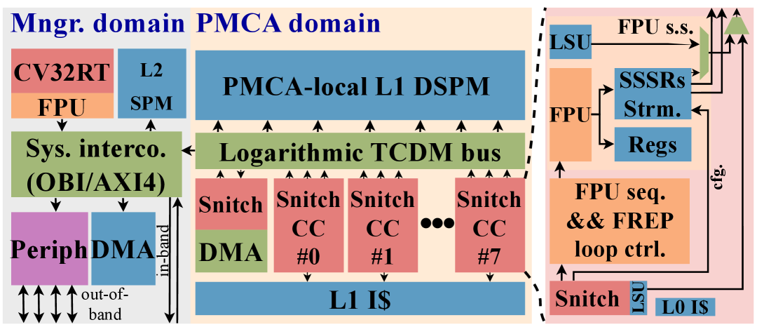
Figure 2: ControlPULP microarchitecture. The Snitch PMCA and core complex with SSSRs and frep extensions are highlighted.

III-A ControlPULP single-core domain

ControlPULP’s manager domain leverages the RTOS task scheduling mechanism to dispatch computationally heavy tasks to the PMCA, thereby accelerating the ETM control algorithm. It oversees the on-chip AXI4-based in-band communication channel, encompassing direct memory access (DMA)-facilitated readouts from PVT sensors, and regulates the allocation of frequencies to the HLC’s PEs according to the control policy. Additionally, it controls the off-chip out-of-band communication channel through dedicated power management peripherals for voltage control.

III-B Snitch PMCA

The Snitch cluster [20] is a RISC-V-based multicore PMCA specialized for energy-efficient floating-point computation. It serves as the LLC’s main compute unit. The cluster features eight RISC-V compute cores, each extended with a hardware loop (frep) and sparsity-capable memory streaming units (SSSRs), described below, to maximize the utilization of its multi-precision floating point unit (FPU). The compute cores share a 32-bank SPM accessed through a single-cycle logarithmic interconnect, as well as an L1 instruction cache. An additional DMA core controls a tightly-coupled DMA engine that facilitates bulk data transfer between the PMCA’s SPM and the manager domain. While the compute cores use a 32-bit instruction set, the FPUs and memory system can be be configured as either 32 or $64\text{\,}\mathrm{bit}$ wide, depending on the requirements of the target application.

III-C SSSRs and hardware loops

Each of the PMCA’s compute cores features three stream semantic registers (SSRs) [20], which map streaming accesses to the shared SPM directly to floating-point registers. SSRs generate stream addresses using dedicated hardware units; this frees the compute core of issuing the loads, stores, and address computations required for streaming memory accesses and enables the near-continuous issuing of useful FPU compute instructions. All three SSRs are capable of up to 4-dimensional strided streams to accelerate compute kernels with regular memory access patterns. We further use the sparse SSR (SSSR) extension so that two of the three SSRs are additionally capable of indirect streams, significantly accelerating the irregular access sequences of sparse workloads like QP. These indexed SSSRs support reading 8-, 16-, 32-, and 64-bit index arrays from SPM to compute addresses for indirect read (gather) or write (scatter) streams accessing SPM.

To autonomously execute repeated sequences of floating-point operations, such as those in iterative loops, the PMCA additionally incorporates the frep (floating-point repetition) extension. frep allows floating-point instruction sequences to be offloaded into a dedicated loop buffer, effectively decoupling FPU instruction issuing from the integer core and thereby enhancing energy efficiency and floating-point utilization.

III-D Memory system hierarchy

The LLC requires more than the few tens of $\mathrm{KiB}$ of memory typically found on low-end microcontrollers. Instead, they are powerful mid-end embedded devices leveraging specialized libraries to handle MIMO interactions and process large volumes of data. This results in memory requirements on the order of $1\text{\,}\mathrm{MiB}$.

ControlPULP’s memory system uses on-chip SPMs, which is still compatible wth on-chip integration at an acceptable cost, thereby reducing access latency, improving predictability, and increasesing the controller’s autonomy within the integrated system. To improve data locality in memory-intensive control algorithms, the PMCA’s local L1 SPM can be scaled up, leaving a smaller shared L2 memory for instruction and data storage in the manager domain. Alternatively, if implementation constraints dictate a smaller SPM size for the PMCA, double-buffering can hide SPM refill latency from the manager domain thanks to the PMCA’s dedicated DMA core (Figure 2).

III-E Real-time control constraints

LLCs for ETM are subject to soft real-time constraints. Misbehavior of the control policy could negatively affect the chip’s performance in case of deadline misses, causing temperature hot spots and overshoots. For these reasons, ControlPULP features streamlined interrupt processing and fast context switch capabilities [8]. A well-designed controller should be fast enough to meet its soft deadlines and minimize response variation (jitter) through hardware-software cooperation. An LLC typically measures the controlled system’s state and applies operating points periodically. In ControlPULP, the FreeRTOS-based ETM application layer is organized in tasks with different priorities and periods responsible for the overall power and thermal policy [8]. Assuming a task set $\Theta$ with periods $\rho_{\theta}$ for $\theta\in\{0,1,...,|\Theta|-1\}$, the least common multiple (LCM) of these periods, denoted as $LCM(\{\rho_{0},\rho_{1},...,\rho_{|\Theta|-1}\})$, is called the hyperperiod [32].

In this work, the MPC controller is encapsulated as a FreeRTOS task $\theta_{MPC}$ with periodicity $\rho_{MPC}$. Hence, the MPC step introduced in Section II-D equals $\rho_{MPC}$. The time to run Algorithm 1 must be less than $\rho_{MPC}$. We call slack the free time left after task execution ends and before a new MPC step starts.

IV MPC controller design and motivation

We first present the power and thermal model for MPC design (Section IV-A). Then, we review the MPC architecture in Section IV-B, and discuss the parameterization of the OSQP solver used throughout the work in Section IV-C. Finally, in Section IV-D, we propose an optimization procedure, termed discrete model pruning (DMP), to increase the sparsity of the problem, thereby reducing its computational complexity and storage requirements. We use the OSQP solver MATLAB interface with the YALMIP framework to conduct the model in the loop (MIL) optimization of the control algorithm. The end-to-end flow down to hardware-aware optimization is presented in Section V-B.

IV-A Thermal and power model for multi-core chiplets

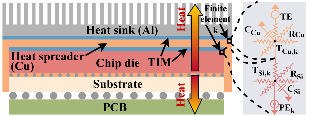
Figure 3: Thermal components with heat propagation flow of an HPC chiplet (left) and lumped parameter circuit of two finite elements from the silicon die and copper heat spreader, respectively (right).

In this section, we introduce the thermal and power model of a multi-core chiplet, which is used to define the optimization problem described in the following Section IV-B. For a detailed treatment, we refer the reader to [33, 34].

The thermal structure is shown Figure 3. It comprises, from top to bottom, a silicon die integrating a grid of $N_{c}=N_{w}\times N_{h}$ PEs, a substrate layer, and the carrier printed circuit board (PCB). The grid is chosen to be square ($N_{w}=N_{h}$). The main heat dissipation path, shown on the right side of Figure 3, passes through a copper heat spreader placed over the active silicon devices and an aluminum heat sink. Thermal interface materials (TIMs) facilitate thermal conductance across layers.

The thermal and power model is derived from the finite element spatial discretization of the partial differential equations (PDEs) describing the silicon and copper heat dissipation. The continuous model is discretized into $h_{C}$ finite elements associated with the $N_{c}$ PEs. An element is modeled with a lumped-parameter circuit, encapsulating the thermal capacitance and resistance of the neighboring materials. Each PE is interpreted as an independent power source $P_{i}$ in the lumped representation. An element has two thermal state variables for the (local) silicon die and metallic heat spreader temperatures. Spatial discretization allows one to obtain a set of ordinary differential equations (ODEs) tractable for control design purposes.

IV-A1 Power model dynamics

The power model dynamics are non-linear. The power source $P_{i}$ associated with PE $i$ is:

$$P_{i} =P_{i,\text{stat}}+P_{i,\text{dyn}}$$ (10)

$$=k_{s_{0}}+(I_{cc,i}V_{i})\cdot\mathcal{K}(T_{Si,i},V_{i})+C_{eff,i}F_{i}V_{i}^{2}$$

where $P_{i,\text{stat}}$, $P_{i,\text{dyn}}$ are the static and dynamic component of the PE’s power consumption. The effective capacitance $C_{\text{eff,i}}$ is correlated to the runtime workload, i.e., the type of instructions $\omega_{i}(t)$ executed by the PE. $\mathcal{K}(T_{Si,i},V_{i})$ is a non-linear mapping that encapsulates the dependency of the static leakage power on the voltage and temperature of the component. In this work, we use an exponential relation based on [35]

$$\mathcal{K}(T_{Si,i},V_{i})=e^{k_{v}V_{i}(t)+k_{T}T_{i}(t)+k_{T_{0}}}$$ (11)

where the $k$ parameters are constant and computed on the critical values of $V_{\text{MAX}}$ and $T_{\text{MAX}}$.

IV-A2 Thermal model dynamics

Collecting the temperatures of all the components shown in Figure 3 for all the $h_{C}$ elements obtained after discretization in a unique vector $T=(T_{Si,1},T_{Cu,1},\ldots,T_{Si,n_{s}},T_{Cu,n_{s}},T_{{Al}})^{T}$, the ODEs for silicon and copper can be written in compact form:

$$\begin{cases}\dot{T}(t)=A_{T}\cdot T(t)+B_{T}\cdot P(t)\\ T_{Si}=C_{T}\cdot T(t)\end{cases}$$ (12)

where $P=(P_{1},\ldots,P_{n_{c}})^{T}$ is the vector of power sources associated with each discrete element, and $A_{T}$, $B_{T}$, $C_{T}$ encapsulate the thermal constants of the lumped representation [33].

The dynamics in Equation 12 and the algebraic power model in Equation 10 jointly characterize the system’s thermal and power behavior.

IV-B MPC Controller architecture

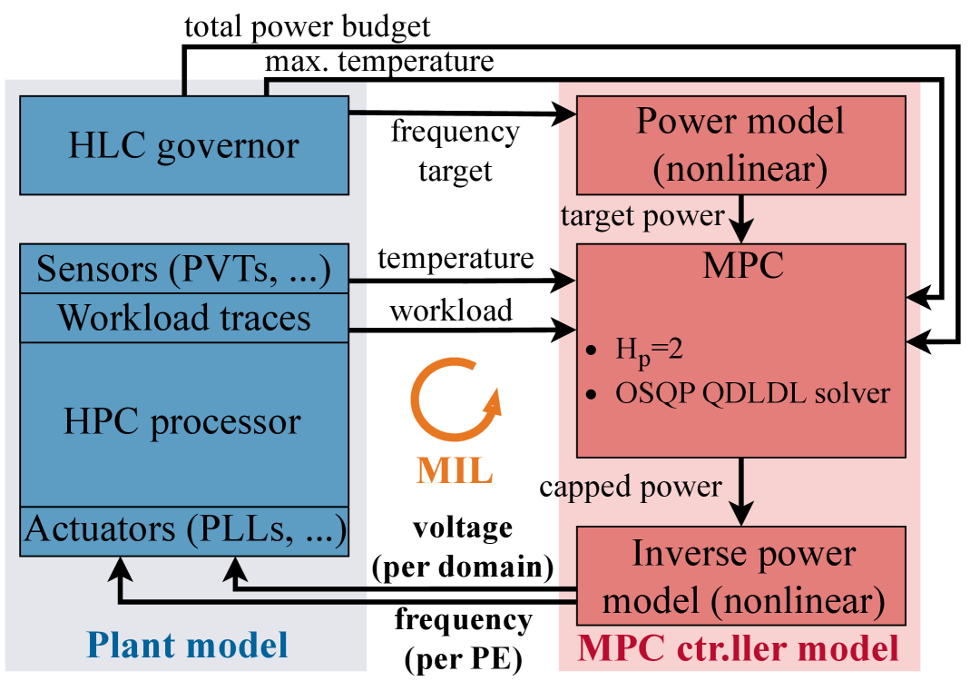
Figure 4: Architectures of ETM MPC controller (right) and plant (left). Both are modeled in MATLAB; the controller architecture is progressively refined using MIL.

Figure 4 illustrates the control loop between the controller (right) and the controlled HPC processor (left) models during MIL design. From a control perspective, the controlled system is referred to as the plant. As described in Section IV-A, the plant is assumed structured as a grid of $N_{c}$ PEs. The control problem for managing the power and temperature of each PE in the grid with a prediction horizon $H_{p}$ is denoted as $\mathtt{PN_{w}\times N_{h}\_{Hp}}$. For instance, $\mathtt{P5\times 5\_H2}$ refers to controlling a $5\times 5$ grid ($N_{c}=25$) with $H_{p}=2$. Since we gather sensor information and dispatch control action to all the PEs through a single controller, this approach is centralized.

The controller operates in three stages, separating non-linearity handling from a centralized linear constrained optimization. First, a power model computes the target power $P_{i}^{*}$ for each PE based on the set-point DVFS commands from the HLC, as well as the measured workload and temperature from the previous interval using on-chip sensors and counters. In the second stage, a linear MPC controller aims to achieve the target power while respecting thermal and power constraints. If constraints are exceeded, the MPC reduces the target power $P_{i}^{*}$ (power-capping). In the third stage, the output powers $P_{i}$ are converted into per-domain voltage and per-PE frequency pairs using an inverse power model and dispatched to PLLs and VRMs actuators. PEs are grouped into power domains $\mathcal{D}_{j}$, each associated to a VRM and its relative power limit [33].

The chosen design for the MPC controller not only aims at capping the temperature of each single PE, as most SoA controllers do [11, 6], but enforces shared power constraints and distributes power among PEs too, representing an advancement over SoA. With this structure, power and thermal constraints are enforced simultaneously, obtaining a globally optimal operating point. An additional global power budget constraint $P_{\text{B}}$ is enforced for the plant. Being shared among the PEs, these power constraints require either a centralized MPC structure or the relaxation of these constraints in a distributed design. The centralized approach thus avoids approximations and delays in effectively enforcing shared power constraints. However, this design choice increases model complexity and computational demands, seen in the dimensional growth of $P$, $A$, $l$, and $u$ in Equation 1.

The MPC constraints can be summed up as follows:

$$\begin{cases}T_{i}\leq T_{\text{L}},\qquad i=1,\dots,N_{c},\\ P_{\text{min}}\leq P_{i}\leq P_{\text{max}},\\ \tsum\slimits@_{i=1}^{N_{c}}P_{i}\leq P_{\text{B}}[t],\\ \tsum\slimits@_{i\in\mathcal{D}_{j}}P_{i}\leq P_{\mathcal{D}_{j}}[t],\quad j=1,\dots,n_{d},\end{cases}$$ (13)

where $T_{\text{L}}$ is the temperature limit and $P_{\text{min}}$ and $P_{\text{max}}$ represent the plant physical limits. In addition to these constraints, the linear thermal model Equation 12 is used as a model constraint.

The optimization function $J$ penalizes deviations from the target power:

$$J=({P^{*}}-{P})^{T}D({P^{*}}-{P}),$$ (14)

where $P$ and $P^{*}$ are the vectors of dispatched and target power for all PEs, and $D$ is a diagonal matrix.

The choice of the prediction horizon $H_{p}$ significantly impacts computational feasibility and controller performance. Longer horizons would better anticipate future dynamics, but in this application, high-amplitude noise [33] causes significant prediction divergence, invalidating the effectiveness of high $H_{p}$ values. An appropriate $H_{p}$ must balance thermal dynamics timing and computational cost. For a control interval $t_{s}\in[1,3]\ \text{ms}$, a range of $H_{p}\in[2,4]$ is a suitable choice based on the fastest thermal time constant [33]. In this setting, high-frequency power spikes can be handled by a parallel, faster control loop reacting to oscillations.

As recalled in Section II-C, a favorable case for fast online MPC arises when the dynamical system and constraints remain constant at each MPC step. In such cases, the matrices $P$ and $A$ in the QP formulation are constant, and any time-varying dynamics can be modeled as updates to the lower and upper bounds $l$ and $u$. This makes the KKT matrix $K$ in Algorithm 1 time-invariant, allowing its symbolic and numerical factorizations to be precomputed and stored only once. Thus, the initial condition in Equation 9 is treated as an equality constraint instead of integrating it into the dynamic equation.

IV-C OSQP parameterization

We use the default OSQP library configuration, selecting the direct QDLD solver with Cholesky decomposition. This is preferred to indirect methods as it is more suitable for very large problems ($N_{nnz}>10^{6}$) [23, 36]. AMD reordering during factorization ensures that fill-ins are minimized, preserving the system’s sparsity and memory efficiency.

For termination, we set the primal and dual tolerances to $\epsilon_{prim}=\epsilon_{dual}=0.01$, achieving a balance between accuracy and computational cost. The convergence-critical ADMM step-size parameters $\rho$ and $\sigma$ are fixed at $\rho=0.1$ and $\sigma=10^{-6}$. The relaxation parameter is set to $\alpha=1.5$.

To further enhance performance on embedded platforms (Section VI-A), we fine-tune the OSQP parameterization during MIL. We combine warm-starting, using the previous iteration’s solution as the initial value (Section II-C), with a fixed max_iter $=15$ to reduce computation time while ensuring constraint satisfaction. Convergence behavior with this iteration limit is discussed in Section V-C. However, in cases with sharp reference changes, additional iterations may be required for convergence.

Moreover, we disable OSQP’s adaptive step-size scheme, which would otherwise adjust $\rho$ based on the primal-to-dual residual ratio at runtime, introducing an expensive online division operation. Lastly, solution polishing is disabled to avoid resolving a linear system with only the active constraints [23], prioritizing execution speed.

IV-D Discrete model pruning

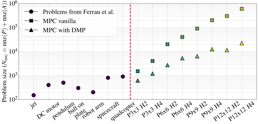
Figure 5: Problem size (Equation 3) of vanilla and pruned MPC for ETM at a varying number of controlled PEs and fixed horizon $H_{p}$=2. DTM uses a cutoff of $0.005$. For comparison, the figure reports the problem size of other MPC problems, reproduced from [24].

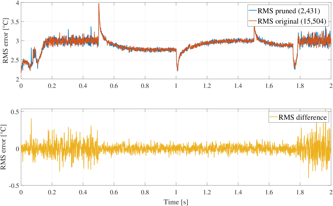
Figure 6: Comparison of vanilla MPC and MPC after DMP on the P99_H2 problem using a MATLAB-based MIL simulation running for $2s$. The top chart shows the RMSE between predicted and measured MPC temperatures over time, while the bottom chart highlights the difference between the two RMSEs. Spikes and offsets in the top chart are due to power budget changes and power model uncertainties, respectively, and are independent of the MPC, hence the RMSE difference is unaffected.

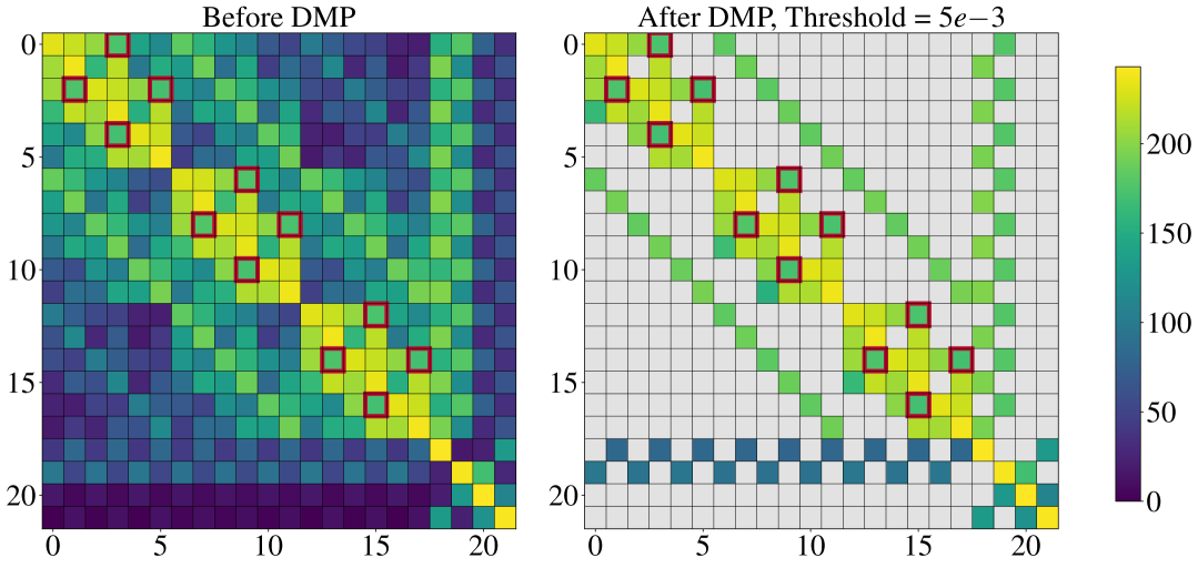
Figure 7: The rationale behind DMP. (Left) vanilla, (right) pruned state matrix $A_{T}$ in Equation 12. We show the problem P33_H2 for readability purposes. Pruned entries are represented in grey. Entries highlighted in red indicate the non-zero values emerged after discretization.

The right-hand side of Figure 5 shows the size of various MPC problems, quantified by the number of non-zero elements ($N_{nnz}$) in the corresponding QP from Equation 3. $N_{nnz}$, along with the number format, significantly influences the memory footprint; data precision is thoroughly discussed in Section V. The solid cross markers in Figure 5 depict a standard problem formulation using the discretized thermal model recalled in Section IV-A. We consider prediction horizons of 2 and 4 to demonstrate the influence of the horizon length on the problem size.

From a thermal perspective, PEs primarily influence their immediate neighbors [37]. Through these direct couplings, their impact propagates across all other PEs, albeit with diminishing amplitude. When discretizing the continuous system, depending on the discretization method and the chosen sampling interval $t_{s}$, additional couplings among PEs in $A_{T}$ in Equation 12 may appear compared to the continuous model structure. By selecting a sufficiently small $t_{s}$ relative to the thermal time constants, these additional couplings exhibit minimal amplitudes and negligible influence. This is because the iterative time-step computation of the thermal model itself effectively captures the thermal influence propagation [37].

We propose a heuristic threshold-based pruning mechanism to exploit these weak, near-zero thermal couplings, thereby reducing the number of non-zero elements in the state matrix and, consequently, the memory footprint. Connections with values above the threshold remain unaltered. Additional measures are taken to preserve the continuous-time structure of the thermal model matrices $A_{T}$ and $B_{T}$, ensuring that the plant dynamics are not truncated. The pruning process is solely intended for memory and computational optimization, without introducing complex approximation criteria. We call the method DMP, as visually illustrated in Figure 7. Given a candidate cutoff threshold, the pruning algorithm computes the RMSEs between the predicted and measured MPC temperature for all system states in the original and pruned model. It then selects the cutoff threshold that minimizes the difference in time between the RMSEs within an allowed range that we set to $0.5\text{\,}\mathrm{\SIUnitSymbolCelsius}$. In this work, we identify a cutoff threshold of $0.005$ for all problems. Figure 6 shows the RMSE evolution for both models of the P99_H2 problem and their difference over time. The pruned thermal model maintains accurate temperature predictions, with the RMSE remaining within the allowed deviation range.

It is important to stress that, despite pruning, MPC remains a more stable and safer alternative to classic PID control. MPC integrates all control variables and constraints into a unified optimization framework by design, whereas PID, as a traditionally single-input single-output method, addresses them separately [11]. Furthermore, it has been shown [38] that the vanilla (non-pruned) MPC outperforms the traditional voting-box PID [10], achieving a worst-case temperature excedance relative to the temperature limit of less than $1.7\text{\,}\mathrm{\SIUnitSymbolCelsius}$, compared to up to $40\text{\,}\mathrm{\SIUnitSymbolCelsius}$ for PID. Similar trends are observed in the average power exceedance relative to the power budget, as well as in the total time exceeding the temperature and power limits [38]. Therefore, the approximation of DMP, bounded within $0.5\text{\,}\mathrm{\SIUnitSymbolCelsius}$, slightly penalizes the original MPC performance but preserves its significant advantages over PID.

DMP reduces the model complexity (and size) from $O(N_{c}^{2})$ to $O(N_{c})$. This reduction is crucial for scaling centralized control as the number of PEs on a silicon die increases. We show this behavior in Figure 5, where the solid triangular markers represent the problem sizes after DMP. As anticipated, the reduction is more pronounced for larger $N_{c}$, resulting in up to 27 decrease in the number of non-zeros for P1212_H4, compared to a 2.5 decrease for P33_H2.

To contextualize these values, the left-hand side of Figure 5 shows typical sizes of embedded QP problems for various applications. Ferrau et al. [24] propose an open-source benchmarking framework for comparing the numerical performance of embedded QP algorithms based on a general MPC formulation. We replicate their results, extracting the problem sizes defined in Equation 3. For the largest evaluated example, P1212_H2, the vanilla MPC formulation is approximately 335 larger than the quadcopter problem from [24]. Despite the complexity reduction achieved by DMP, the pruned MPC model still remains over 13 larger.

This section highlighted the significant memory challenges of the analyzed problem. The next Section IV-E addresses these challenges from an execution time perspective.

IV-E Impact of MPC on execution time

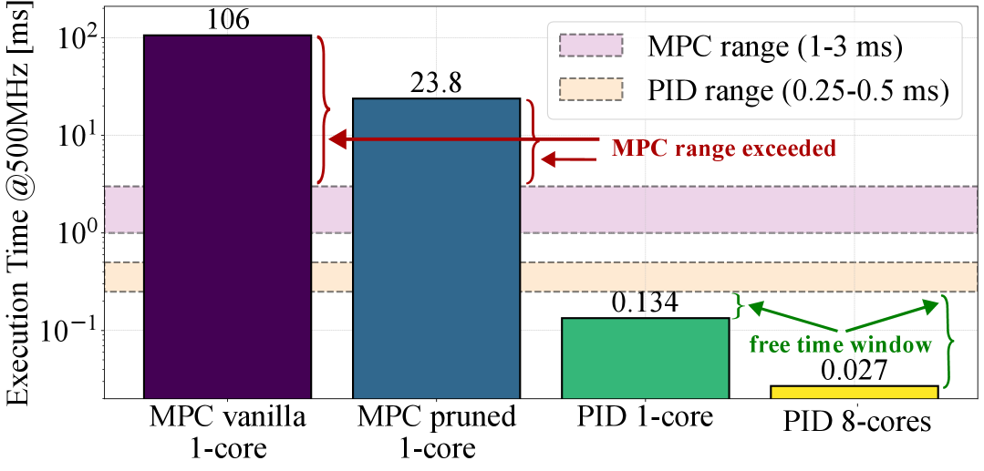
Figure 8: Execution time of vanilla and pruned MPC and PID’s ETM policies on ControlPULP at $500\text{\,}\mathrm{MHz}$. Data for PID are taken from [8] when controlling 72 PEs. MPC is executed for 15 iterations until convergence using vanilla OSQP for P99_H2 problem, i.e., 81 PEs.

We contextualize the high computational demands of MPC for ETM by providing a quantitative comparison of the execution time compared to a PID control policy, which represents the current SoA in this application domain [8]. The comparison is shown in Figure 8. All algorithms are executed on ControlPULP in different configurations. For the MPC, the QP solver runs 15 iterations. PID results are taken from [8]. The light yellow and orange areas indicate the permissible execution ranges for PID and MPC algorithms. PID is computationally lightweight and generally faster than MPC. SoA controllers for power and thermal management can execute one control policy iteration in $250500\text{\,}\mathrm{\SIUnitSymbolMicro s}$ (hyperperiod range, Section III-E). Its optimization on the PMCA further increases available slack (green arrows in Figure 8). In contrast, both vanilla and DMP MPC fail to meet their deadline (red arrows in Figure 8) by a large margin, being 35.3 and 7.9 slower than the $3\text{\,}\mathrm{ms}$ upper bound of the permissible range discussed in Section IV-B. Together with the problem size comparison in Figure 5, this further motivates the need for hardware-software co-optimization to streamline and accelerate the execution of expensive ETM predictive control schemes on resource-constrained systems. In the following section, we detail our methodology to achieve this goal.

V Hardware-software co-optimization and acceleration methods

We first outline the optimization metrics and framework considered for efficient deployment of the MPC solver algorithm on the target multi-core embedded platform (LABEL:, V-A and V-B). We then present and discuss the proposed hardware-aware optimizations to accelerate the algorithm and maximize resource utilization. The optimization scope includes numerical precision considerations (Section V-C), ParSPL for multi-core acceleration and code generation of the SpTRSV (Section V-D), and leveraging the LLC’s SSSRs and hardware loop extensions (Section V-E).

V-A Optimization metrics

The following optimization metrics are essential for efficient deployment on a resource-constrained system:

Memory Footprint

The goal is twofold: (i) to keep data close to the compute resources in low-latency on-chip SPM memories, as accessing off-chip dynamic random access memory (DRAM) increases latency and reduces the autonomy of the LLC, and (ii) to ensure that the compiled algorithm size remains below $1\text{\,}\mathrm{MiB}$ as discussed in Section III. Preserving sparsity in the state matrices is crucial to achieving this goal. This motivates the use of DMP during MIL and AMD reordering during Cholesky factorization.

Execution speed

To meet the real-time constraints described in Sections III-E and IV-D and illustrated in Figure 8, optimizations must focus on solving the QP problem within or below the target MPC step time.

Hardware utilization

Factors such as synchronization overhead, parallelization inefficiencies, and data non-locality prevent the full utilization of compute units, wasting execution cycles on stalls or non-compute operations and thus reducing execution speed and energy efficiency. We aim to maximize FPU utilization of the eight PMCA cores through AOT scheduling and the use of SSSRs (Section III).

Energy-efficiency

The power manager’s energy profile is critical, as its overhead can impact the overall HPC die performance [39]. Maximizing compute utilization of the control algorithm enhances its energy efficiency ($\mathrm{FLOP}\text{/}\mathrm{s}\text{/}\mathrm{W}$), thereby reducing the LLC’s chip-level impact.

V-B Optimization framework

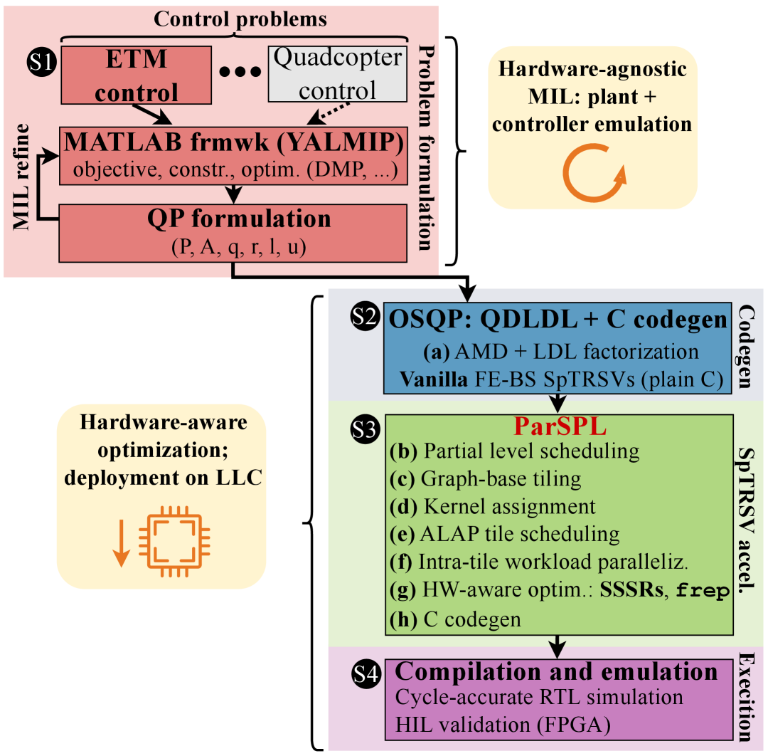
Figure 9: Optimization framework stages highlighted from hardware-agnostic MIL to hardware-aware multi-core scheduling, optimization, and deployment of the MPC control algorithm on the target LLC.

Figure 9 shows the progression from hardware-agnostic MIL to hardware-aware deployment and hardware-in-the-loop (HIL) emulation.

In the MIL simulation phase [baseline=(char.base)][white,shape=circle,fill=ieee-dark-black-100,draw,inner sep=1pt] (char) S1;, the QP solver is validated independently of the hardware platform. For instance, DMP (Section IV-D) is evaluated and applied at this stage. This level of abstraction relies on MATLAB and YALMIP, which has native support for the OSQP solver.

Then, the deployment stage progresses toward a hardware-aware design space that considers LLC-specific instruction set architecture (ISA) extensions, memory, and computing resources. First, OSQP’s native code generation capabilities translate the high-level MATLAB representation of the QP solver into embedded C [29], as shown in [baseline=(char.base)][white,shape=circle,fill=ieee-dark-black-100,draw,inner sep=1pt] (char) S2;. At this stage, AMD reordering and LDL factorization are performed by OSQP; the resulting triangular $L$ matrix is generated in compressed sparse column (CSC) format. Second, the ParSPL scheduler further preprocesses the matrix $L$ to achieve extremely fast and efficient multi-core execution of the SpTRSV in the FE and BS phases of QDLDL (stage [baseline=(char.base)][white,shape=circle,fill=ieee-dark-black-100,draw,inner sep=1pt] (char) S3;). We detail ParSPL in Section V-D. Finally, to further increase resource utilization on the embedded platform, the deployed code harnesses the hardware-specific SSSR extensions available on the LLC’s PMCA (Section III).

This framework automatically generates the optimized solver code for Algorithm 1. Before compilation and deployment on the target platform, the solver is encapsulated as a FreeRTOS task with periodicity larger than the minimum MPC step size achievable after optimization (Section III-E) and integrated within the control firmware.

V-C Data precision format

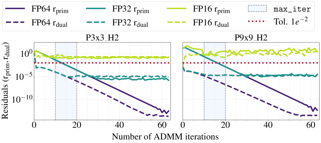
Figure 10: Primal and dual residual evolution for P33_H2 and P99_H2 at different precision formats. We use OSQP Python’s interface with cold starting on a desktop-grade x86 machine. The solver is executed for $\texttt{max\_iter}=64$ iterations. We highlight a feasible range for max_iter in [10-25] (light-blue region).

As mentioned in Section IV-D, data precision impacts the memory footprint in embedded MPC deployments. On embedded platforms, lower precision formats such as float32 (FP32), float16 (FP16), and float8 (FP8) are commonly used to minimize storage consumption. However, lower precision can introduce numerical errors for iterative solvers like OSQP, affecting constraint satisfaction and solver convergence [21, 40].

Figure 10 illustrates the evolution of $r_{\text{prim}}$ and $r_{\text{dual}}$ at different data precisions for two problems of different sizes, P33_H2 and P99_H2. We leverage OSQP’s Python interface on a desktop-grade x86 machine. Algorithm 1 is executed for max_iter $=64$ iterations, with tolerances $\epsilon_{\text{prim}}=\epsilon_{\text{dual}}=0.01$ serving as termination criteria. We observe that float64 (FP64) delivers the best convergence behavior for primal and dual residuals. FP32 performs slightly worse, while FP16 experiences numerical instability early in the solver progression. Because of the poor convergence behavior of FP16, we did not explore FP8.

In the following, we uniformly adopt FP32 across the entirety of Algorithm 1. This choice provides a balanced tradeoff between computational precision and memory efficiency, mitigating the risks of numerical instability. Other alternatives could be explored, such as a mixed-precision approach where only critical components of Algorithm 1 essential for numerical stability and convergence are computed in higher precision to reduce the memory footprint further.

V-D ParSPL: AOT scheduling and parallelism extraction

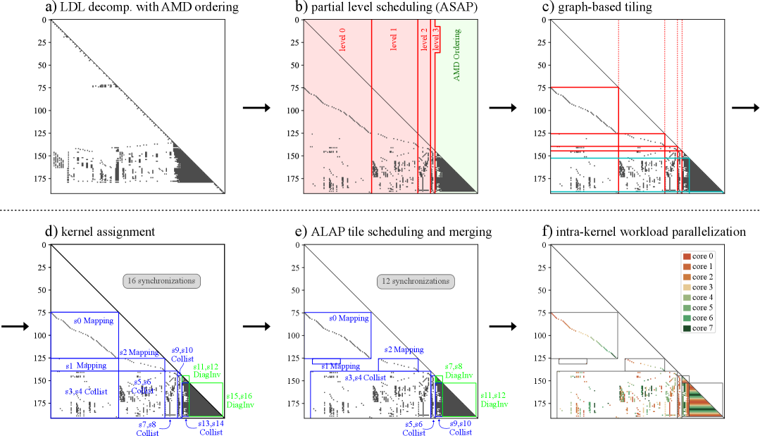
Figure 11: ParSPL steps applied to the lower triangular matrix $L$ for the problem P33_H2. The starting point in (a) is the LDL decomposition. In (b), partial level scheduling extracts inherent parallelism from the sparsity pattern. Strongly dependent components (i.e., denser regions) are retained in the original AMD ordering to preserve the beneficial structure, particularly along the diagonal. These strongly interconnected components are separated in (c) using a graph-based approach. Cuts from partial level scheduling are shown in red, while graph-based tiling cuts are in cyan. The resulting tiles in (c) are merged and assigned to one of three kernels in (d) using static rules in a black-box manner without considering specific data dependencies within and between tiles. In step (d), the tile region, kernel name, and synchronization steps are visualized. To further reduce synchronizations, tiles are dynamically scheduled using ALAP and merged into shards in (e). This exposes concurrency based on the actual sparsity pattern and the dependencies arising from the non-zero data locations. Finally, in (f), intra-shard workloads are distributed across the 8 PMCA cores.

The most computationally expensive step in Algorithm 1, and the most challenging to parallelize on a multi-core system with limited resources, is the linear system solver described in 3. In contrast, the updates in 4, 5, 7 and 6 of Algorithm 1 are dense, component-wise-separable vector operations, accounting for only $11\text{\,}\mathrm{\char 37\relax}$ of the total solver pass execution time during single-core execution. Since the triangular matrix $L$ after AMD reordering is constant, Algorithm 1 repeatedly solves the linear system with a changing right-hand side vector using FE and BS until termination. The need for multiple solver passes and the limited resources of the target platform justify the extensive precomputation and preprocessing adopted by ParSPL to maximize the figures of merit discussed in Section V-A.

LDL decomposition with AMD ordering

Since any column-based approach in FE is transposed to a row-based approach in BS, we store the lower triangular matrix $L$ according to the CSC representation, and the following discussion will focus exclusively on $L$. Figure 11-a illustrates the structure of $L$ after AMD reordering for the P33_H2 problem, chosen to improve readability.

Two key aspects of FE and BS pose challenges to achieving high execution performance on single- and multi-core systems. First, the index arrays in the CSC representation of $L$ lead to indirect and irregular memory access patterns, negatively impacting compute utilization. Second, both algorithms exhibit inherent dependencies: FE follows a fan-out pattern, where updates propagate to multiple entries, while BS follows a fan-in reduction structure. These dependencies hinder straightforward parallelization and necessitate extensive synchronization to manage shared data across the computing cores, significantly impacting performance as we will show in Section VI-A.

To efficiently parallelize the triangular solver, ParSPL uses a hybrid method, combining partial level scheduling and tiling of $L$. Figures 11b-f show the process steps.

Partial level scheduling (ASAP)

Level scheduling is a common technique to extract parallelism in a SpTRSV by rearranging the matrix into a sequence of levels [41]. A level is a set of independent columns (or equations) that can be processed in parallel. Levels are executed sequentially, as they depend on one another. Sparser columns with fewer dependencies are prioritized and rearranged to be processed as soon as possible (ASAP) to create the levels.

As a result, level scheduling removes all unnecessary synchronizations across the PMCA compute cores. However, its effectiveness diminishes as independent columns thin out across levels, leading to two primary challenges. The first is the increased synchronization demands as the algorithm proceeds because deeper columns become denser and more likely to have blocking dependencies with others; this results in many small blocking levels with fewer members. The second is the disruption of dense sub-triangular structures near the lower diagonal, created by AMD reordering, which are easier to parallelize when densely populated.

To address the limitations of full level scheduling, we use partial level scheduling, discarding levels with fewer columns than a set threshold similarly to [42]. Columns in the discarded levels retain the original AMD ordering. The choice of the threshold is based on heuristics and derived by varying the problem size. In the target application considered in this work, at most the first four levels typically satisfy the threshold constraint. Figure 11-b depicts $L$ after this step.

Graph-based tiling

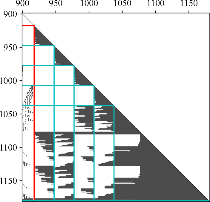
Figure 12: Graph-based tiling for P88_H2. Red lines denote cuts derived from partial level scheduling, while cyan lines indicate cuts introduced by graph-based tiling.

Following partial level scheduling, $L$ is automatically partitioned into a few large, irregular tiles that minimize inter-tile synchronization while maximizing intra-tile parallelism. Partial level scheduling naturally divides a portion of the $L$ matrix into tiles, as shown in Figure 11-c with solid vertical and horizontal red lines. For the remaining AMD-ordered part, we use graph-based partitioning to extract the dense triangular sub-matrices along the diagonal. The remaining $L$ matrix is interpreted as an adjacency graph where nodes correspond to the columns/rows indices; an edge connects two nodes $i$ and $j$ if $l_{ij}$ is non-zero. The edge weight for an element $l_{ij}$ is defined as $\frac{1}{(i-j)^{2}}$, assigning greater importance to elements near the diagonal and less to those farther away. Using the Ford-Fulkerson algorithm and the Max-Flow Min-Cut theorem, the graph is partitioned into two subgraphs by cutting along the weakest links. The obtained cuts are shown in cyan in Figure 11-c. This process identifies dense sub-diagonal triangular regions and is applied recursively until a heuristic termination criterion. The collection of all cuts defines the tiling boundaries. To highlight the importance of graph-based partitioning for larger problems, Figure 12 illustrates the process on the P88_H2 problem, where dense sub-triangular matrices dominate.

Kernel assignment

Tiles are assigned to specialized kernels. Decomposing the vanilla QDLDL algorithm into heterogeneous kernels allows one to leverage the diverse sparsity structures and data representations of the tile topologies introduced by the previous steps.

We identify four kernel types, each with two variants for FE and BS. Mapping is used for regions where each row and each column at most contain one element. An element corresponds to a floating-point multiply and accumulate operation that is independent both in FE and BS, so it can be trivially computed concurrently. Diaginv is used for dense triangles along the diagonal. The insight behind this kernel is that inverting an (almost) dense triangular matrix results again in an (almost) dense triangular matrix. The matrix inversion is computed AOT to eliminate all synchronizations at runtime. The corresponding matrix-vector multiplication is well-known and parallelizable. The diagonal inverse multiplication, i.e., the multiplication by $D^{-1}$ from the LDL decomposition after FE, is a variant of Diaginv. Finally, Collist, or column list, deals with regular sparse data stored in CSC format and is used for all remaining rectangular tiles. The rectangular shape ensures disjoint memory read and write locations, avoiding any synchronizations.

After the initial assignment, horizontally aligned tiles requiring the same kernel type are merged using static rules to minimize unnecessary inter-tile synchronizations (see Figure 11-d). Kernels with conflicting memory write during FE or BS are assigned a second synchronization step to accommodate a reduction.

ALAP tile scheduling and merging

Stage (e) performs inter-tile scheduling and merging, assuming tiles are black boxes. In Figure 11-f, the actual data dependencies within and between tiles are considered based on the non-zero locations. For each tile, the data-dependent read and write accesses are determined. This information is then used to build a directed acyclic graph (DAG) of tiles that are scheduled ALAP. The choice over ASAP is illustrated next. Looking at the $L$ matrix, ASAP schedules vertical tiles as they share variables to be read before computation. In contrast, horizontal tiles share variables to be written to a region in the right-hand-side (RHS) vector after computation. As horizontal Collist tiles were merged in Figure 11-d using static rules, the ASAP potential is largely exhausted, whereas ALAP is found to significantly decrease the number of synchronizations. An example is a reduction from 53 to 34 in P99_H2. The tiles obtained by ParSPL are denoted shards as they can overlap, are non-rectangular, and do not have to cover the entire matrix.

Intra-shard workload parallelization

While shards are processed sequentially, the data within a shard is inherently designed for full parallelization, enabled by prior optimizations. Therefore, workload distribution to the PMCA compute cores is trivial and depicted in Figure 11-f, where each core represents a color. ParSPL automatically generates C code from the resulting scheduling (Figure 9), with appropriate data structures and data types that minimize memory footprint.

V-E SSSRs and hardware loops

As shown in Figure 9, the kernels identified during the SpTRSV optimization are further optimized using dedicated PMCA’s hardware extensions to boost hardware utilization and performance of the compute cores, i.e., SSSRs and frep (Section III). Both memory streams and regular loops are programmed ahead of computing. We introduce the average streaming length (SL) as $\mathrm{SL}=\frac{nnz(L)}{\mathrm{\#synchr.}}$. SL is the key metric in determining SSSR impact and resulting FPU utilization and indicates the average number of non-zeros per shard. The lower $nnz(L)$ (the sparser the matrix), the lower SL and the benefits of accelerated indirect memory streams. Hence, techniques oriented towards memory efficiency, like DMP, negatively affect the inherent parallelism of the problem. Similarly, the fewer synchronizations required for parallel execution, the greater the performance improvement.

In the next section, we provide an exhaustive evaluation of the presented methodology Section V-A.

VI Deployment and Evaluation

We evaluate the performance of the optimized solver using the metrics and methodology outlined in Section V. To assess improvements in execution speed and hardware utilization on the PMCA, we conduct cycle-accurate RTL simulations (stage [baseline=(char.base)][white,shape=circle,fill=ieee-dark-black-100,draw,inner sep=1pt] (char) S4; in Figure 9). The memory footprint is analyzed using LLVM 15.0.0, targeting RV32IMAFCXsssrXfrep. Finally, we perform gate-level assessments of power consumption, energy, and area efficiency of the controller using GlobalFoundries’ GF12LP+ node with a 13-metal-stack, 7.5-track standard cell library targeting the typical corner ($25\text{\,}\mathrm{\SIUnitSymbolCelsius}$, $0.8\text{\,}\mathrm{V}$).

VI-A Functional Performance

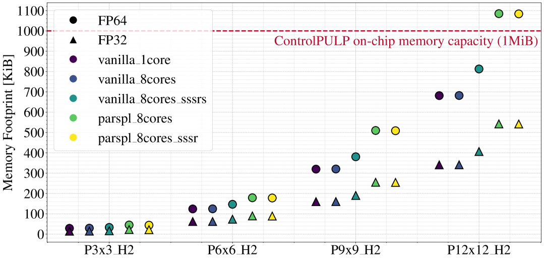
Figure 13: Memory footprint of various MPC problems with FP64 (circle) and FP32 (triangle) data precisions, optimized with different strategies (color-coded) after compilation for ControlPULP. All problems apply DMP in MIL. Both data precisions allow to stay well within the LLC memory constraints discussed in Section III.

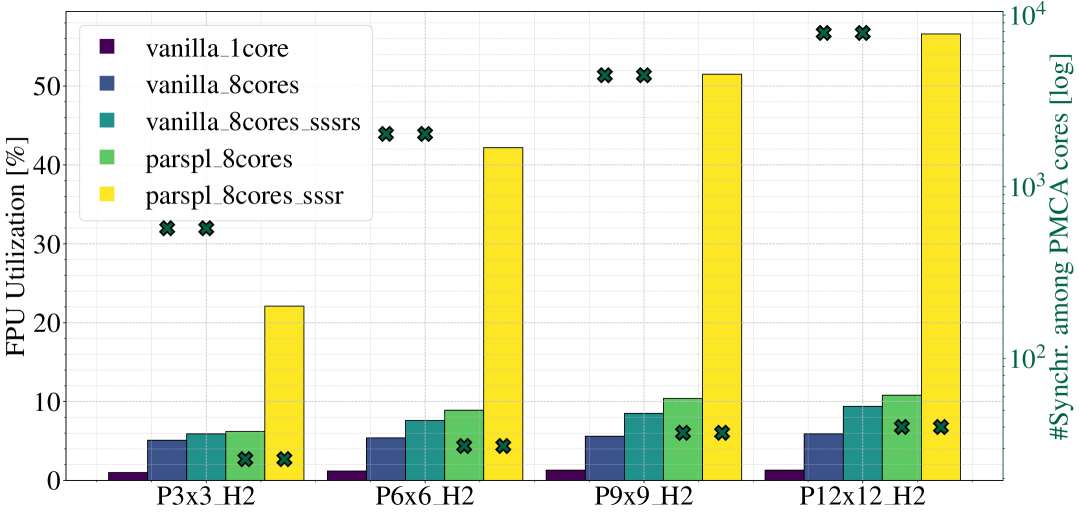
Figure 14: (Bars) FPU utilization of 3 during MPC execution. (Points) Number of synchronization steps required among the PMCA compute cores. Both metrics apply to a problem size with different optimization methods.

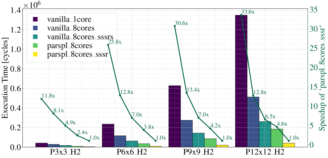
Figure 15: (Left) MPC execution speed for different problems and optimization methods in clock cycles. The chart considers one iteration of the linear system solver (3 in Algorithm 1). (Right) Speedup of the best method (parspl_8cores_sssr) compared to the others.

We evaluate problems of sizes $N_{w}=N_{h}=[3,6,9,12]$, i.e, grids with up to 144 PEs on the same silicon die. For each problem, we assess various optimization methods: vanilla single-core (vanilla_1core, used as a baseline reference), naive multi-core parallelization across the columns of $L$ (vanilla_8cores), and ParSPL.

Memory Footprint

Figure 13 illustrates the memory footprint in $\mathrm{KiB}$ for FP64 (circle) and FP32 (triangle) precisions. All problems apply DMP. Optimization methods that utilize SSSRs employ a $16\text{\,}\mathrm{bit}$ index to reduce overhead. The density of the triangular matrix $L$ ranges from $1.88\text{\,}\mathrm{\char 37\relax}$ for the smallest to largest evaluated problems.

For problem sizes $N_{w}=N_{h}>9$, ParSPL introduces a memory overhead of approximately $100\text{\,}\mathrm{KiB}$ to $300\text{\,}\mathrm{KiB}$ compared to the baseline OSQP. In the FE phase, this overhead arises from the matrix inversions applied by ParSPL to submatrices near the lower diagonal of $L$, which increase the number of fill-ins relative to the original $L$ (Figure 11). The majority of the overhead, however, stems from the current implementation, which stores the inverted triangular dense matrices in a rectangular format, including the upper triangular zeros. While storing only the triangular part could reduce memory usage, it would degrade the utilization of SSSRs.

Overall, a problem at scale like P1212_H2 fits in less than $550\text{\,}\mathrm{KiB}$ with FP32 precision. This provides a significant margin for controlling larger systems — over 200 PEs on a single silicon die — without exceeding the storage constraint discussed in Section III.

Hardware Utilization

The bars in Figure 14 depict the average FPU utilization across the eight PMCA cores during one solver iteration. We observe the beneficial impact of ParSPL coupled with SSSRs and hardware loops, enabling efficient acceleration of both affine and indirect memory streams (parspl_8cores_sssr). This configuration achieves $56.6\text{\,}\mathrm{\char 37\relax}$ FPU utilization, approximately 43 higher than the single-core implementation using vanilla OSQP and 6 higher than the naive column-based parallelization (vanilla_8cores_sssr).

The utilization improvement in a multi-core setting mainly correlates with the reduced synchronization steps between the PMCA compute cores. The points in Figure 14 show the evolution of synchronization steps for each optimization method. To provide a more detailed analysis, we concentrate on P1212_H2. The single-core case incurs no synchronization overhead, as it is single-threaded. The plain vanilla parallelization method incurs around 7900 synchronizations, while ParSPL reduces this to about 40.

When SSSRs and hardware loops are used, execution improves FPU utilization for both parallelization methods but at different scales: 1.6 for the vanilla approach and 5.2 for ParSPL. This gap arises due to the longer average SL of $L$ introduced by ParSPL (Section V-E). As the SL grows with the inverse of the synchronization count, the benefits of SSSRs are significantly enhanced when fewer synchronizations are required. For instance, on P1212_H2, the SL is $7.9$ for vanilla_8cores and $1538.2$ for parspl_8cores.

Execution Time (1 iteration)

We report the latency of Algorithm 1 in clock cycles. We first focus on the sparse linear system solver at 3 of  Algorithm 1 as it is the bottleneck of the computation (Section V-D). The left-hand side of Figure 15 illustrates the execution time for one iteration. The right-hand side shows the speedup of parspl_8cores_sssr, the most performant optimization method, against others. Compared to the vanilla single-core OSQP case, ParSPL is 11.8 faster for smaller problems like P33_H2 and up to 33.6 faster for the largest evaluated problem, P1212_H2.

parspl_8cores achieves a high parallelization efficiency across the eight PMCA compute cores, delivering a 7.2 speedup over single-core performance, close to the theoretical maximum. In contrast, vanilla_8cores reaches only a 5.2 speedup. Similarly, parspl_8cores_sssr outperforms vanilla_8cores_sssr with nearly 5 faster execution. These results arise from the superior parallelism extracted by ParSPL, where the number of dependent sub-kernels requiring synchronization steps is minimized, while their inner workload is divided into independent chunks across the PMCA’s compute cores (Figure 11-f).

End-to-end Performance

To demonstrate the end-to-end solution time improvement introduced by ParSPL, we recall the chart in Figure 8, which emphasizes the limitations of vanilla MPC when controlling 81 PEs (P99_H2) on an embedded single-core LLC. Using parspl_8cores_sssr and terminating the solver after $\texttt{max\_iter}=15$, the sparse linear system solver in 3 takes approximately 307k clock cycles. The dense vector operations involved in Algorithm 1 (4, 5, 7 and 6) are accelerated through static distribution of equal chunks to each computing core, coupled with direct stream and loop acceleration in hardware, eliminating the overhead of memory and control operations. This reduces the execution time of these operations from 2490k clock cycles of vanilla single-core OSQP to just 37k clock cycles, approximately 67 faster. Assuming a conservative controller operating frequency of $500\text{\,}\mathrm{MHz}$, the total latency of a solver pass for this problem becomes $0.69\text{\,}\mathrm{ms}$. This result drastically reduces the time required to solve the QP optimization problem online, enabling very short MPC steps under $1\text{\,}\mathrm{ms}$. Even allowing the solver to converge for more iterations would still leave a reasonable free time window within the MPC step. This enables an online ETM control policy to manage a few hundred PEs using a centralized embedded controller, and achieves more than $1\text{\,}\mathrm{kHz}$ control bandwidth.

VI-B Area and Energy efficiency

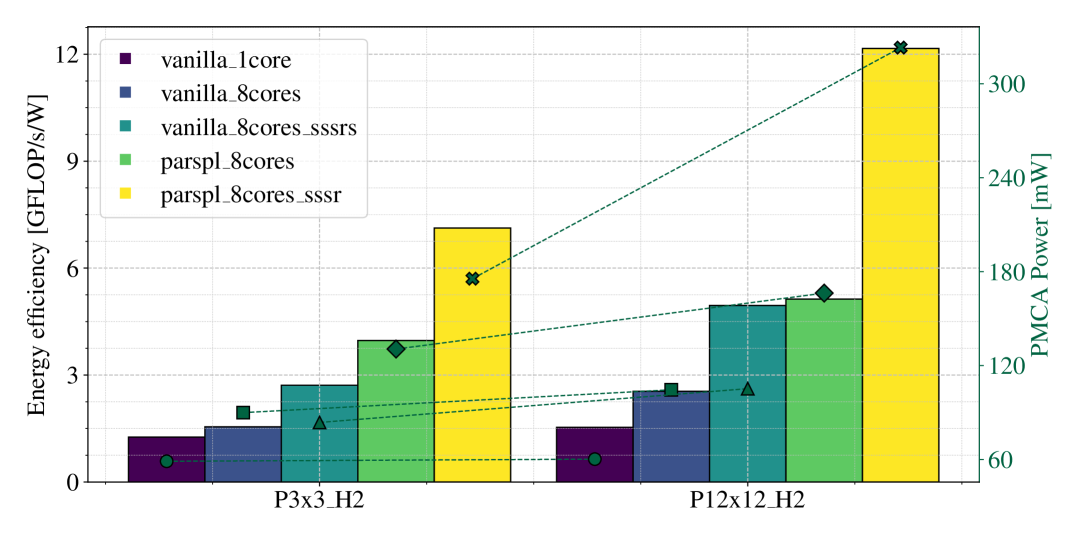
Figure 16: The energy efficiency of the linear system solver in 3, Algorithm 1 for the smallest and largest evaluated problems in different optimization scenarios.

Area Efficiency

We implement the design using Synopsys Fusion Compiler at $500\text{\,}\mathrm{MHz}$ under typical conditions ($25\text{\,}\mathrm{\SIUnitSymbolCelsius}$, $0.8\text{\,}\mathrm{V}$). We configure ControlPULP with $128\text{\,}\mathrm{KiB}$ of L2 SPM and $1\text{\,}\mathrm{MiB}$ of L1 SPM for the manager and PMCA domains, respectively. A modern HPC die, fabricated in a similar advanced technology node, typically has an area ranging from $200800\text{\,}{\mathrm{mm}}^{2}$ [43, 16], depending on the packaging technology, number of PEs, and their microarchitecture. In such a large system, the area overhead of our controller, assuming a single instance for centralized control, is a negligible $0.21.5\text{\,}\mathrm{\char 37\relax}$. Given the growing number of PEs integrated in each processor generation and the trend toward compute chiplets, even a scale-out approach using multiple controllers to manage different compute domains — such as a multi-PMCA configuration — remains justified due to its minimal area overhead.

Energy Efficiency

Figure 16 shows the estimated energy efficiency (points) and power consumption (bars) of the LLC’s PMCA when solving, at $32\text{\,}\mathrm{bit}$ data precision, one iteration of the ADMM’s linear system solver on the P33_H2 and P1212_H2 problems. Results are shown across all optimization scenarios discussed in Section VI-A. Power estimates are obtained using Synopsys PrimeTime. As expected, the median power consumption of the PMCA increases when using SSSRs. ParSPL introduces additional overhead due to higher FPU and L1 SPM utilization. However, the SSSR-optimized version of ParSPL achieves energy efficiency improvements of up to 2.4 compared to the vanilla ParSPL, and up to 7.9, 2.4, and 4.8 compared to vanilla single-core and vanilla parallelization with and without SSSRs, respectively. The largest problem instance, P1212_H2, in its most optimized configuration, maintains a total power consumption below $325\text{\,}\mathrm{mW}$. This is nearly three orders of magnitude lower than that of traditional HLC-centric approaches for executing MPC policies, which typically consume power in the range of tens of Watts due to the overhead of the OS stack and the inherently power-hungry architectures of conventional application-class PEs. These approaches are reviewed in the next Section VII.

VII Related Work

We initially examine SoA MPC schemes for ETM (Section VII-A). Then, in Section VII-B, we explore works targeting fast online MPC in a wide range of control scenarios and problem scales, mostly relying on the ADMM algorithm. Section VII captures the main aspects discussed in this section.

TABLE I: QP acceleration solutions for various applications and control problems using MPC.

ieee-dark-black-100

MPC appl. profile

Algorithm (best referenced configuration)

Deployment Platform

MPC Performance

ieee-dark-black-100

Class

Referenced application

QP Sol. Method

Solver

Exploits sparsity?

Data precision

Pred. horizon

HW topology

HW platform

Mem. hierarchy

Target freq. [$\mathrm{MHz}$]

Peak Power [$\mathrm{W}$]

Mem. footprint [$\mathrm{KiB}$]

Time to solve

Best sample time

ieee-dark-black-40        Online MPC for various control applications

ieee-dark-black-40 Alavilli et al.    [19]

Emb.

6-DOF quadr.

ADMM

tinyMPC

✗

FP32

15-20

MCU

STM32F405

$192\text{\,}\mathrm{KiB}$ DRAM + $1\text{\,}\mathrm{MiB}$ flash

168

$<$0.1

$<$192

$<$2ms-n.a.

2ms

Bitjoka et al. [44]

Emb.

DC motor

FNLQDMC

n.a.

✗

Custom

2

MCU

Arduino Due

$96\text{\,}\mathrm{KiB}$ SPM + $512\text{\,}\mathrm{KiB}$ flash

84

n.a.

83

0.8-2.9ms

3-8ms

Chaber et al. [45]

Emb.

Servo

FGPC FDMC

Custom

✗

FP32

50 50

MCU

STM32F746

$320\text{\,}\mathrm{KiB}$ SPM + $1\text{\,}\mathrm{MiB}$ flash

216

$<$0.6

n.a.

$11\text{\,}\mathrm{\SIUnitSymbolMicro s}$ $584\text{\,}\mathrm{\SIUnitSymbolMicro s}$

$250\text{\,}\mathrm{\SIUnitSymbolMicro s}$ 1ms

Jerez et al. [40, 17]

Emb.

AFM control

FG ADMM (expl.)

Custom

✗

Fix. point

16

DSA

Virtex6 FPGAa Spartan6 FPGAa

-

400 230

n.a.

n.a.

4.9-8.9$\mu$s 0.5-0.9$\mu$s

1-1.5$\mu$s

Jerez et al. [46]

Emb.

Spring-mass

Int.-point + Newton

Custom

✓

Fix. point

4 9

DSA

Virtex6 FPGA

-

400

n.a.

n.a.

371ms

388ms

Malouche et al. [47]

Emb.

Robot

GPC

Custom

✗

FP32

20

MCU

STM32F407

$192\text{\,}\mathrm{KiB}$ SPM + $1\text{\,}\mathrm{MiB}$ flash

168

$<$0.07

10.6

$4.9\text{\,}\mathrm{\SIUnitSymbolMicro s}$

5.3ms

Sabo et al. [48]

Emb.

Double integrator

Primal-dual

Custom

✓

Fix. point

9

DSA

Digil. Nexys 4

-

100

n.a.

n.a.

n.a.

n.a.

Vouzis et al. [49]

Emb.

Rot. antenna Glucose regul.

Newton

Custom

✗

LNS

20 5

DSA

Virtex4 FPGA

2 BlockRAMs

50

n.a.

n.a.

0.45ms 0.68ms

n.a. few min

Wills et al. [50]

Emb.

14th-order harmon.

Active-set

Custom

✗

Customc

12

DSA

Stratix III FPGA

-

70

n.a.

n.a.

30$\mathrm{\SIUnitSymbolMicro s}$

200$\mathrm{\SIUnitSymbolMicro s}$

Wang et al. [26]

HPC

Oscill. masses Supply chain Random

Int.-point

Custom

✓

n.a.

10/30

Desk. CPU

Athlon

n.a.

3000

35 (TDP)

n.a.e

$<$1ms $<$12msb $<$25ms

5ms 12ms 25ms

Schubiger et al. [36]

HPC

Random

ADMM

cuOSQP (PCG)

✓

FP32 FP64

n.a.

GP-GPU

i9-9900K + RTX2080Ti

$64\text{\,}\mathrm{GiB}$ DDR4 $11\text{\,}\mathrm{GiB}$ VRAM

3600

250 (TDP of RTX)

n.a.

100ms-90s 200ms-100s

200ms-100s

ieee-dark-black-40        Online MPC for energy and thermal management of HPC processors

ieee-dark-black-40 Bartolini et al.    [11]

HPC

ETM distrib. 1 PE

Active-set

n.a.

✗

FP64

2

Desk. CPU

n.a.

n.a.d

2400

n.a.

n.a.

4.69$\mathrm{\SIUnitSymbolMicro s}$f

1-10ms

Tilli et al. [6]

HPC

ETM distrib. 1 PE

n.a.

n.a.

✗

FP64

2

Desk. CPU

Intel i7 8th gen.

n.a.e

4600

95 (TDP)

n.a.

3$\mathrm{\SIUnitSymbolMicro s}$f

1ms

Wang et al. [13]

HPC

ETM centr. 16 PEs

Least-square

lsqlin

✗

n.a.

8

Desk. CPU

Xeon X5365

n.a.e

3000

150 (TDP)

n.a.

n.a.

40ms

Maity et al. [51]

Emb.

ETM centr. 4 PEs

Heur. beam search

n.a.

✗

FP32

n.a.

DSA

Odroid XU4

n.a.

2000

n.a.

n.a.

Few ms

n.a.

This work

Emb.

ETM centr. 81 PEs g

ADMM

OSQP (QDLDL)

✓

FP32 FP64

2

Spec. paral. MCU

ControlPULP

$<$$1\text{\,}\mathrm{MiB}$ SPM h

500

$<$0.325 i

600 i

0.69ms i

$<$1ms i

ieee-dark-black-100

• The papers report only potential performance and resource usage without effective measurements.

• The paper reports average time per iteration; no explicit sample time is given.

• Custom floating-point format with 7 exponent bits and a mantissa in the range [7,15].

• Data from Fig. 9 of [11] obtained on a dual-core desktop processor.

• The paper lacks details on the exact memory hierarchy configuration, despite it being a commercial processor.

• Time per single controlled PE.

• We report the largest problem evaluated in this work

• Relies only on on-chip SPM hierarchy for manager domain and PMCA. See Section III.

• Refers to controlling 81 PEs, which fits the memory constraint of $1\text{\,}\mathrm{MiB}$.

VII-A MPC for ETM

Due to MPC’s complexity, classical works leverage the computational capabilities of the controlled out-of-order, application-class PEs to execute the controller, which becomes part of the HLC governor (Figure 1-a). Bartolini et al. [11] propose an MPC architecture limited to thermal capping that leverages a distributed approach to address the complexity of centralized methods. Taking advantage of the parallel architecture of the multi-core system on chip (SoC), each PE computes autonomously its future frequency in line with the incoming workload requirements. The deployment platform, a desktop central processing unit (CPU) operating at $3\text{\,}\mathrm{GHz}$, enables online solving of the QP problem using active-set methods in approximately $5\text{\,}\mathrm{\SIUnitSymbolMicro s}$ per PE, achieving sampling intervals of $110\text{\,}\mathrm{ms}$. Similarly, Tilli et al. [6] propose a two-layer distributed MPC framework combining a decentralized thermal capping layer for guaranteed feasibility and a distributed MPC layer for performance optimization. The approach is software-based, and evaluation is performed executing the controller on last-generation Intel processors. Wang et al. [13], instead, adopts a centralized strategy. It provides experimental data for controlling up to 16 PEs, using a $3\text{\,}\mathrm{GHz}$ Intel Xeon X5 and achieving an MPC sample time below $5ms$. In contrast, our centralized scheme controls 5 more PEs with 10 lower execution time and running the controller’s cores at 6 lower frequency, three orders of magnitude smaller power consumption, and at least two orders of magnitude smaller memory footprint. Maity et al. [51] propose a thermally optimizing scheduler for CPU/GPU mobile architectures like the Odroid-XU4. They use a lightweight heuristic beam search, executed by a quad-core Cortex-A7 LLC, to minimize peak temperature over a hyper-period. Scalability is not addressed, as their ETM policy manages a quad-core Cortex-A15 and a 6-shader Mali GPU in a fixed configuration.

These works focus on controller design, formulation, and reliability for the ETM problem, but omit details on the QP solver or problem data structure (sparse/dense). Their HLC-centric approach for thermal and power capping also incurs high overhead from power-hungry, OS-based software stacks, as shown in Section VII.

VII-B Online MPC: from high-end to embedded systems

Early efforts to make online MPC viable on embedded systems focus on accelerating sparse optimization methods. For instance, the seminal work from Wang et al. [26] fully exploits the problem sparsity with an interior-point method, enabling a linear growth of the number of operations per MPC stepwith $H_{p}$, rather than cubic. This strategy allows for tackling fairly large problems — a few hundred to thousands of state variables and constraints — with sample times of $525\text{\,}\mathrm{ms}$, over 100 faster than a dense optimizer. While the approach inspired today’s SoA, such as OSQP, it does not target embedded platforms directly and evaluates the control problems on a $3\text{\,}\mathrm{GHz}$ desktop machine.

One way to tackle MPC’s computational complexity is to design domain-specific accelerators (DSAs) to accelerate the QP solver pass. Vouzis et al. [49] propose an auxiliary co-processor with a microcode interface to accelerate the computationally intensive steps of Newton’s algorithm. To reduce memory footprint, a single 16-bit logarithmic number system (LNS) unit iterates over the input data and stores intermediate results in local memories. However, the evaluated problems are limited in size, with fewer than six decision variables ($n$) and constraints ($m$), making them 16 smaller than the smallest P33_H2 problem analyzed in this work ($n=95\;\mathrm{and}\;m=97$). Wills et al. [50] employ a similar approach using an active-set method, which entails expensive matrix inversion computation. In [40, 17], Jerez et al. present hardware circuits to accelerate both FG and ADMM methods with dense dynamics, while in [46], they exploit sparsity to achieve a $75\text{\,}\mathrm{\char 37\relax}$ memory reduction and a 6.5 speedup over an equivalent software implementation running on a CPU. The accelerators proposed in [40, 17] show that sample intervals in the range of $11.5\text{\,}\mathrm{\SIUnitSymbolMicro s}$ using FG and $525\text{\,}\mathrm{\SIUnitSymbolMicro s}$ using ADMM are feasible on field-programmable gate arrays (FPGAs) clocked at $150\text{\,}\mathrm{MHz}$, with a QP size of $n=704$ and $m=544$ (smaller than P33_H2 with $n=1310\;\mathrm{and}\;m=1312$).

All discussed DSAs have been implemented on FPGAs, reporting excellent execution times for fast MPC. However, memory footprint is often not analyzed, performance on the deployed device is only estimated [17], and metrics like power consumption and incurred area are omitted, as accurate evaluation would require ASIC implementation.

Recent research initiatives, notably those centered around the OSQP solver, have rejuvenated interest in ADMM methods. Alavilli et al. [19] propose TinyMPC, a QP solver that accelerates and compresses ADMM, combined with linear quadratic regulators (LQRs), for extremely resource-constrained systems. TinyMPC’s key approach is the pre-computation (caching) of the Riccati solution of the LQR problem, equivalent to the primal update in ADMM’s Equation 5. With this approach, it attains a speedup of up to 8.8 over vanilla OSQP on a single-core MCU while adhering to stringent memory limitations ($<$ $512\text{\,}\mathrm{KiB}$) using random, small- and medium-scale problem instances (up to $n=696\;\mathrm{and}\;m=490$). TinyMPC could be a promising candidate for ETM as the memory usage and execution time exhibit more linear growth than vanilla OSQP at varying $n$, $m$, and $H_{p}$. LQR policies for thermal management of HPC processors have been previously studied [52]. They prioritize maintaining a uniform thermal profile rather than minimizing power consumption, and lack explicit threshold constraints on the chip maximum temperature in their optimization formulation. Instead, constraints like frequency bounds and thermal limits are addressed externally through post-optimization adjustments. This reliance on external corrections limits the effectiveness of LQR under heavy workloads, as it cannot dynamically account for nonlinearities or spatial and temporal thermal gradients, which are essential for efficient thermal management in modern HPC processors.

Schubiger et al. [36] focus instead on accelerating OSQP on large-scale problems ($N_{nnz}\geq 10^{4}$). They propose cuOSQP, a CUDA-optimized solver for NVIDIA graphic processing units (GPUs) based on the preconditioned conjugate gradient (PCG) indirect method to solve the ADMM linear system, achieving a peak speedup of $15\times$ and $5\times$ over single-threaded, vanilla QDLDL OSQP and multi-threaded, MKL-Pardiso OSQP, respectively, for the largest evaluated problem ($N_{nnz}=10^{8}$) on a NVIDIA RTX2080Ti. However, their assessment shows that vanilla QDLDL OSQP is roughly $10\times$ faster than PCG-based cuOSQP for $N_{nnz}<10^{6}$, the same problem range evaluated in this work. While this supports our choice of a QDLDL-based approach, indirect methods remain promising candidates for very large ETM control problems involving thousands of PEs, a scale not yet achieved by any major commercial vendor.

Several other works have addressed the mapping of fast MPC algorithms on commercial MCUs [45, 47, 44]. Despite achieving sub-$\mathrm{ms}$ solution times with a memory footprint in the tens of $\mathrm{KiB}$, the tackled problems are small, with tens of decision variables and constraints. Furthermore, conventional MCUs rely on memory hierarchies with an external flash alongside on-chip SPMs or caches. While external memory is an option for embedded LLCs, a self-contained, on-chip memory hierarchy improves responsiveness and autonomy as we explain in Section III.

The comparative analysis shows that our hardware/software co-optimization framework (Section V-B) outperforms SoA MPC schemes for ETM in HPC processors, requiring fewer computing resources and storage while delivering low-power execution and high energy efficiency at a small fraction of the HPC processor die area. It also competes with fast MPC methods deployed on various architectures like MCUs, DSAs, and GPUs and validated on other control applications. This efficiency stems from leveraging AOT pre-computation and parallelization derived from the problem matrix’s sparsity pattern. Moreover, unlike fixed-function accelerators, our hardware is flexible and can be adapted to different algorithms and problems, helping avoid premature obsolescence that often affects hardwired accelerators.

VIII Conclusion

In this work, we presented a comprehensive framework for implementing MPC for energy and thermal management of HPC processors using a resource-constrained, multi-core, embedded RISC-V LLC. The proposed method addressed the computational challenges of solving quadratic programming problems in real-time by leveraging the ADMM algorithm and optimizing the SoA OSQP solver. To achieve this goal, we presented several key optimization techniques, including a threshold-based pruning algorithm to optimize the model memory usage and ahead-of-time scheduling with the ParSPL framework to extract inherent parallelism from the sparse triangular system solved at runtime. The optimized MPC framework achieved significant reductions in execution time, memory footprint, and energy consumption, enabling the control of up to 144 processing elements on a single silicon die with sub-millisecond latency within a few hundred of $\mathrm{KiB}$. This solution outperforms SoA HLC-centric methods that routinely require desktop-grade computing resources, demonstrating the feasibility of delegating advanced ETM policies to embedded, on-chip controllers. The approach was validated through extensive cycle-accurate simulations, paired with a physical implementation of the LLC using an advanced GlobalFoundries’ GF12LP+ node for power estimation, achieving up to 33 speedup and 7.9 energy efficiency gains in solving SpTRSVs compared to single-core OSQP, with a memory footprint below $1\text{\,}\mathrm{MiB}$, well within the LLC constraints, and a power consumption below $325\text{\,}\mathrm{mW}$.

Alessandro Ottaviano received the B.Sc. in Physical Engineering from Politecnico di Torino, Italy, and the M.Sc. in Electrical Engineering as a joint degree between Politecnico di Torino, Grenoble INP-Phelma and EPFL Lausanne, in 2018 and 2020, respectively. He is currently pursuing a Ph.D. degree in the Digital Circuits and Systems group of Prof. Benini. His research interests include embedded system design and energy-efficient computing.

Andrino Meli received his BSc and MSc degrees in electrical engineering and information technology from ETH Zurich in 2022 and 2024, respectively. He is currently a research assistant at the Institute for Integrated Systems. His research interests include control systems, numerical optimization, parallel algorithm design and linear system solvers.

Paul Scheffler received his BSc and MSc degrees in electrical engineering and information technology from ETH Zurich in 2018 and 2020, respectively. He is currently pursuing a Ph.D. degree in the Digital Circuits and Systems group of Prof. Benini. His research interests include hardware acceleration of sparse and irregular workloads, on-chip interconnects, manycore architectures, and high-performance computing.

Giovanni Bambini studied Automation Engineering at the University of Bologna, with a focus on control theory and microcontrollers. He earned a PhD in Electronic Engineering, specializing in modeling and control of HPC CPUs. During his doctoral research, he actively contributed to the European Processor Initiative (EPI), working on thermal and power management control, chip modeling and design. His research interests include advanced control theory, modeling and identification, and real-time firmware development.

Robert Balas received his BSc and MSc degrees in electrical engineering and information technology from ETH Zurich in 2015 and 2017, respectively. He is currently pursuing a Ph.D. degree in the Digital Circuits and Systems group of Prof. Benini. His research interests include real-time computing, compilers, and operating-systems.

Davide Rossi received the Ph.D. degree from the University of Bologna, Bologna, Italy, in 2012. He has been a Post-Doctoral Researcher with the Department of Electrical, Electronic and Information Engineering “Guglielmo Marconi,” University of Bologna, since 2015, where he is currently an Associate Professor. His research interests focus on energy-efficient digital architectures. In this field, he has published more than 100 papers in international peer-reviewed conferences and journals.

Andrea Bartolini (Member, IEEE) received the Ph.D. degree from the University of Bologna, Bologna, Italy, in 2013. He is an Associate Professor with the Department of Electrical, Electronic and Information Engineering Guglielmo Marconi, University of Bologna, Bologna, Italy. He has published more than 120 papers in peer-reviewed international journals and conferences and several book chapters with focus on dynamic resource management—ranging from embedded to large-scale HPC systems.

Luca Benini (F’07) holds the chair of Digital Circuits and Systems at ETH Zurich and is Full Professor at the Università di Bologna. Dr. Benini’s research interests are in energy-efficient computing systems design, from embedded to high-performance. He has published more than 1000 peer-reviewed papers and five books. He is a Fellow of the ACM and a member of Academia Europaea.

References

- [1] Z. Guo, Y. Tang, J. Zhai, T. Yuan, J. Jin, L. Wang, Y. Zhao, and R. Li, “A survey on performance modeling and prediction for distributed dnn training,” IEEE Trans. on Parallel and Distrib. Syst., vol. 35, no. 12, pp. 2463–2478, 2024.
- [2] R. Stocks, E. Palethorpe, and G. M. J. Barca, “Multi-gpu ri-hf energies and analytic gradients-toward high-throughput ab initio molecular dynamics,” J. Chem. Theory Comput., vol. 20, no. 17, pp. 7503–7515, 2024.
- [3] S. Cheng, X. Zhao, G. Lu, J. Fang, T. Zheng, R. Wu, X. Zhang, J. Peng, and Y. You, “Fastfold: Optimizing alphafold training and inference on gpu clusters,” in Proc. of the 29th ACM SIGPLAN Annu. Symp. on Princ. and Pract. of Parallel Program., ser. PPoPP ’24. New York, NY, USA: Association for Computing Machinery, 2024, p. 417–430.
- [4] W.-c. Feng and K. Cameron, “The green500 list: Encouraging sustainable supercomputing,” Computer, vol. 40, no. 12, pp. 50–55, 2007.
- [5] A. Vassighi and M. Sachdev, “Thermal runaway in integrated circuits,” IEEE Trans. on Device and Mater. Rel., vol. 6, no. 2, pp. 300–305, 2006.
- [6] A. Tilli, E. Garone, C. Conficoni, M. Cacciari, A. Bosso, and A. Bartolini, “A two-layer distributed mpc approach to thermal control of multiprocessor systems-on-chip,” Control Eng. Pract., vol. 122, p. 105099, 2022.
- [7] Arm, “Power control system architecture,” 2023. [Online]. Available: https://developer.arm.com/documentation/den0050/d/?lang=en
- [8] A. Ottaviano, R. Balas, G. Bambini, A. Del Vecchio, M. Ciani, D. Rossi, L. Benini, and A. Bartolini, “Controlpulp: A risc-v on-chip parallel power controller for many-core hpc processors with fpga-based hardware-in-the-loop power and thermal emulation,” Int. J. of Parallel Program., vol. 52, no. 1, pp. 93–123, Apr 2024.
- [9] A. Grover, “Modern system power management: Increasing demands for more power and increased efficiency are pressuring software and hardware developers to ask questions and look for answers.” Queue, vol. 1, no. 7, p. 66–72, oct 2003.
- [10] T. Rosedahl, M. Broyles, C. Lefurgy, B. Christensen, and W. Feng, “Power/Performance Controlling Techniques in OpenPOWER,” in High Perform. Comput., J. M. Kunkel, R. Yokota, M. Taufer, and J. Shalf, Eds. Cham: Springer International Publishing, 2017, pp. 275–289.
- [11] A. Bartolini, M. Cacciari, A. Tilli, and L. Benini, “Thermal and energy management of high-performance multicores: Distributed and self-calibrating model-predictive controller,” IEEE Trans. on Parallel and Distrib. Syst., vol. 24, no. 1, pp. 170–183, 2013.
- [12] X. Sun, A. Boora, R. Pamula, C.-H. Huang, D. Peña-Colaiocco, and V. S. Sathe, “Model predictive control of an integrated buck converter for digital soc domains in 65nm cmos,” in 2020 IEEE Symp. on VLSI Circ., 2020, pp. 1–2.
- [13] X. Wang, K. Ma, and Y. Wang, “Adaptive power control with online model estimation for chip multiprocessors,” IEEE Trans. on Parallel and Distrib. Syst., vol. 22, pp. 1681–1696, 2011. [Online]. Available: https://api.semanticscholar.org/CorpusID:11497998
- [14] T. L. Group, “SiPearl Develops ARM HPC Chip,” 2020. [Online]. Available: https://www.linleygroup.com/newsletters/newsletter_detail.php?num=6227&year=2020&tag=3
- [15] AMD, “Epyc 7004 Genoa,” 2022. [Online]. Available: https://en.wikichip.org/wiki/amd/cores/genoa
- [16] NVIDIA, “Nvidia grace cpu superchip,” 2023. [Online]. Available: https://www.nvidia.com/en-us/data-center/grace-cpu-superchip/
- [17] J. L. Jerez, P. J. Goulart, S. Richter, G. A. Constantinides, E. C. Kerrigan, and M. Morari, “Embedded online optimization for model predictive control at megahertz rates,” IEEE Trans. on Autom. Control, vol. 59, no. 12, pp. 3238–3251, 2014.
- [18] T. Salzmann, E. Kaufmann, J. Arrizabalaga, M. Pavone, D. Scaramuzza, and M. Ryll, “Real-time neural mpc: Deep learning model predictive control for quadrotors and agile robotic platforms,” IEEE Robot. and Automat. Lett., vol. 8, no. 4, p. 2397–2404, Apr. 2023.
- [19] K. Nguyen, S. Schoedel, A. Alavilli, B. Plancher, and Z. Manchester, “Tinympc: Model-predictive control on resource-constrained microcontrollers,” in 2024 IEEE Int. Conf. on Robot. and Automat. (ICRA), 2024, pp. 1–7.
- [20] P. Scheffler, F. Zaruba, F. Schuiki, T. Hoefler, and L. Benini, “Sparse stream semantic registers: A lightweight isa extension accelerating general sparse linear algebra,” IEEE Trans. on Parallel and Distrib. Syst., vol. 34, no. 12, p. 3147–3161, Dec. 2023.
- [21] S. Boyd, N. Parikh, E. Chu, B. Peleato, and J. Eckstein, “Distributed optimization and statistical learning via the alternating direction method of multipliers,” Found. Trends Mach. Learn., vol. 3, no. 1, p. 1–122, jan 2011.
- [22] J. Nocedal and S. J. Wright, Numer. Optim., 2nd ed. New York, NY, USA: Springer, 2006.
- [23] B. Stellato, G. Banjac, P. Goulart, A. Bemporad, and S. Boyd, “Osqp: an operator splitting solver for quadratic programs,” Math. Program. Comput., vol. 12, no. 4, p. 637–672, Feb. 2020.
- [24] D. Kouzoupis, A. Zanelli, H. Peyrl, and H. J. Ferreau, “Towards proper assessment of qp algorithms for embedded model predictive control,” in 2015 Eur. Control Conf. (ECC), 2015, pp. 2609–2616.
- [25] M. S. K. Lau, S. P. Yue, K. V. Ling, and J. M. Maciejowski, “A comparison of interior point and active set methods for fpga implementation of model predictive control,” in 2009 Eur. Control Conf. (ECC), 2009, pp. 156–161.
- [26] Y. Wang and S. Boyd, “Fast model predictive control using online optimization,” IEEE Trans. on Control Syst. Technol., vol. 18, no. 2, pp. 267–278, 2010.
- [27] B. O’Donoghue, G. Stathopoulos, and S. Boyd, “A splitting method for optimal control,” IEEE Trans. Control Syst. Technol., vol. 21, no. 6, pp. 2432–2442, 2013.
- [28] G. Stathopoulos, H. Shukla, A. Szucs, Y. Pu, and C. N. Jones, Operator Splitting Methods in Control. Now Foundations and Trends, 2016.
- [29] G. Banjac, B. Stellato, N. Moehle, P. Goulart, A. Bemporad, and S. Boyd, “Embedded code generation using the osqp solver,” in 2017 IEEE 56th Annu. Conf. on Decis. and Control (CDC). IEEE Press, 2017, p. 1906–1911.
- [30] P. R. Amestoy, T. A. Davis, and I. S. Duff, “Algorithm 837: Amd, an approximate minimum degree ordering algorithm,” ACM Trans. Math. Softw., vol. 30, no. 3, p. 381–388, sep 2004.
- [31] H. Najibi, A. Levisse, G. Ansaloni, M. Zapater, M. Vasic, and D. Atienza, “Thermal and voltage-aware performance management of 3-d mpsocs with flow cell arrays and integrated sc converters,” IEEE Trans. on Comput.-Aided Des. of Integr. Circuits and Syst., vol. 42, no. 1, pp. 2–15, 2023.
- [32] I. Ripoll and R. Ballester-Ripoll, “Period selection for minimal hyperperiod in periodic task systems,” IEEE Trans. on Comput., vol. 62, no. 9, pp. 1813–1822, 2013.
- [33] G. Bambini, A. Ottaviano, C. Conficoni, A. Tilli, L. Benini, and A. Bartolini, “Modeling and controlling many-core hpc processors: an alternative to pid and moving average algorithms,” ACM Trans. Auton. Adapt. Syst., Sep. 2024, just Accepted.
- [34] H. Sultan, A. Chauhan, and S. R. Sarangi, “A survey of chip-level thermal simulators,” ACM Comput. Surv., vol. 52, no. 2, apr 2019.
- [35] A. Bartolini and D. Rossi, “Advances in power management of many-core processors,” in Many-Core Computing: Hardware and Software. IET, 2022, ch. 8, pp. 191–213.
- [36] M. Schubiger, G. Banjac, and J. Lygeros, “Gpu acceleration of admm for large-scale quadratic programming,” J. of Parallel and Distrib. Comput., vol. 144, pp. 55–67, 2020.
- [37] F. Beneventi, A. Bartolini, A. Tilli, and L. Benini, “An effective gray-box identification procedure for multicore thermal modeling,” IEEE Trans. on Comput., vol. 63, no. 5, pp. 1097–1110, 2014.
- [38] G. Bambini, “Mastering power control in hpc cpus: A journey through modeling, algorithms, and hardware insights,” Ph.D. thesis, University of Bologna, 2025, to appear. Expected to be available at: https://amslaurea.unibo.it/. Temporary access link: https://iis-nextcloud.ee.ethz.ch/s/Eda4TRnqBdszoj3.
- [39] V. Gupta, P. Brett, D. Koufaty, D. Reddy, S. Hahn, K. Schwan, and G. Srinivasa, “The forgotten ’uncore’: on the energy-efficiency of heterogeneous cores,” in Proc. of the 2012 USENIX Conf. on Annu. Tech. Conf., ser. USENIX ATC’12, USA, 2012, p. 34.
- [40] J. L. Jerez, P. J. Goulart, S. Richter, G. A. Constantinides, E. C. Kerrigan, and M. Morari, “Embedded predictive control on an fpga using the fast gradient method,” in 2013 Eur. Control Conf. (ECC), 2013, pp. 3614–3620.
- [41] Y. Saad, Iterative Methods for Sparse Linear Systems, 2nd ed. Philadelphia, PA: SIAM, 2003.
- [42] A. M. Bradley, “A hybrid multithreaded direct sparse triangular solver,” in Proc. of the 2016 SIAM Workshop on Combinatorial Scientific Comput. (CSC), 2016, pp. 13–22.
- [43] E. Rotem, A. Yoaz, L. Rappoport, S. J. Robinson, J. Y. Mandelblat, A. Gihon, E. Weissmann, R. Chabukswar, V. Basin, R. Fenger, M. Gupta, and A. Yasin, “Intel alder lake cpu architectures,” IEEE Micro, vol. 42, no. 3, pp. 13–19, 2022.
- [44] M. Ndje, L. Bitjoka, A. T. Boum, D. J. Fotsa Mbogne, L. Buşoniu, J. C. Kamgang, and G. V. Tchané Djogdom, “Fast constrained nonlinear model predictive control for implementation on microcontrollers,” IFAC-PapersOnLine, vol. 54, no. 4, pp. 19–24, 2021, 4th IFAC Conf. on Embedded Syst., Comput. Intell. and Telematics in Control CESCIT 2021.
- [45] P. Chaber and M. Ławryńczuk, “Fast analytical model predictive controllers and their implementation for stm32 arm microcontroller,” IEEE Trans. on Ind. Inform., vol. 15, no. 8, pp. 4580–4590, 2019.
- [46] J. L. Jerez, G. A. Constantinides, and E. C. Kerrigan, “An fpga implementation of a sparse quadratic programming solver for constrained predictive control,” in Proc. of the 19th ACM/SIGDA Int. Symp. on Field Programmable Gate Arrays, ser. FPGA ’11, 2011, p. 209–218.
- [47] I. Malouche, A. K. Abbes, and F. Bouani, “Automatic model predictive control implementation in a high-performance microcontroller,” in 2015 IEEE 12th Int. Multi-Conf. on Syst., Signals & Devices (SSD15), 2015, pp. 1–6.
- [48] J. R. Sabo and A. A. Adegbege, “A primal-dual architecture for embedded implementation of linear model predictive control,” in 2018 IEEE Conference on Decision and Control (CDC), 2018, pp. 1827–1832.
- [49] P. D. Vouzis, L. G. Bleris, M. G. Arnold, and M. V. Kothare, “A system-on-a-chip implementation for embedded real-time model predictive control,” IEEE Trans. Control Syst. Technol., vol. 17, no. 5, pp. 1006–1017, 2009.
- [50] A. G. Wills, G. Knagge, and B. Ninness, “Fast linear model predictive control via custom integrated circuit architecture,” IEEE Trans. Control Syst. Technol., vol. 20, no. 1, pp. 59–71, 2012.
- [51] S. Maity, R. Roy, A. Majumder, S. Dey, and A. R. Hota, “Future aware dynamic thermal management in cpu-gpu embedded platforms,” in 2022 IEEE Real-Time Syst. Symp. (RTSS), 2022, pp. 396–408.
- [52] F. Zanini, D. Atienza, C. N. Jones, L. Benini, and G. De Micheli, “Online thermal control methods for multiprocessor systems,” ACM Trans. Des. Autom. Electron. Syst., vol. 18, no. 1, jan 2013.