Euclid preparation

The Euclid mission aims to measure the positions, shapes, and redshifts of over a billion galaxies to provide unprecedented constraints on the nature of dark matter and dark energy. Achieving this goal requires a continuous reassessment of the mission’s scientific performance, particularly in terms of its ability to constrain cosmological parameters, as our understanding of how to model large-scale structure observables improves. In this study, we present the first scientific forecasts using CLOE (Cosmology Likelihood for Observables in Euclid), a dedicated Euclid cosmological pipeline developed to support this endeavour. Using advanced Bayesian inference techniques applied to synthetic Euclid-like data, we sample the posterior distribution of cosmological and nuisance parameters across a variety of cosmological models and Euclid primary probes: cosmic shear, angular photometric galaxy clustering, galaxy-galaxy lensing, and spectroscopic galaxy clustering. We validate the capability of CLOE to produce reliable cosmological forecasts, showcasing Euclid’s potential to achieve a figure of merit for the dark energy parameters $w_{0}$ and $w_{a}$ exceeding 400 when combining all primary probes. Furthermore, we illustrate the behaviour of the posterior probability distribution of the parameters of interest given different priors and scale cuts. Finally, we emphasise the importance of addressing computational challenges, proposing further exploration of innovative data science techniques to efficiently navigate the Euclid high-dimensional parameter space in upcoming cosmological data releases.

1 Introduction

Euclid, a medium-class mission of the European Space Agency (ESA) under the Cosmic Vision 2015–2025 programme, is designed to investigate the accelerated expansion of the Universe, attributed to dark energy (Perlmutter et al. 1999; Garnavich et al. 1998; Riess et al. 1998), and to explore the nature of dark matter (Feng 2010). It also aims to probe the initial conditions that seeded cosmic structure and to test the limits of general relativity (Laureijs et al. 2011). Following its successful launch on July $1^{\rm st}$ 2023, Euclid has begun mapping the cosmos in unprecedented detail, focusing on the large-scale structure (LSS) and compiling one of the most extensive galaxy catalogues to date.

As a cornerstone of contemporary cosmology, Euclid will complement and extend results from current surveys to test the concordance cosmological model, $\Lambda\mathrm{CDM}$, where cosmic acceleration is driven by a cosmological constant $\Lambda$ (Heymans et al. 2021; Abbott et al. 2022; DESI Collaboration: Adame et al. 2024b). The mission also targets the $w_{0}w_{a}\mathrm{CDM}$ extension, where dark energy is treated as a barotropic fluid with a redshift-dependent equation of state $w(z)\equiv p/\rho c^{2}$. In particular, we adopt the Chevallier–Polarski–Linder (CPL) parametrisation, a widely used Maclaurin expansion for $w(z)$ (Chevallier & Polarski 2001; Linder 2003).

$$w(z)=w_{0}+w_{a}\,\frac{z}{1+z}\;,$$ (1)

where $w_{0}$ is the present day ($z=0$) value of the EoS, while $w_{a}$ measures how fast it evolves with redshift. In $\Lambda\mathrm{CDM}$, $w_{0}=-1$ and $w_{a}=0$. In particular, we aim to quantify the performance of Euclid in discerning the nature of the dark Universe by comparing the so-called dark energy figure of merit ($\mathrm{FoM}$), which is defined as the inverse square root of the covariance-matrix determinant for the dark energy parameters $w_{0}$ and $w_{a}$ (Wang 2008),

$${\rm FoM}=\frac{1}{\sqrt{\det{\rm Cov}(w_{\rm 0},w_{a})}}\;.$$ (2)

A larger $\mathrm{FoM}$ indicates a more precise measurement of the dark energy properties. For this reason, it is crucial to increase, as much as possible, the available data used for the analysis to decrease the statistical uncertainty associated with these parameters.

As the Euclid survey progresses and the covered area expands, it becomes essential to refine cosmological forecasts to ensure the readiness of Bayesian analysis pipelines for the missions scientific exploitation. The initial forecasts outlined in the Euclid Definition Study Report (Laureijs et al. 2011) set the stage for the missions cosmological objectives, but recent developments call for a reassessment. First, our improved understanding of the theoretical complexity involved in modelling large-scale structure observablessuch as cosmic shear, angular galaxy clustering, galaxy-galaxy lensing, and spectroscopic clusteringnow demands more accurate treatments. These models must incorporate systematic effects, which introduce a large number of nuisance parameters and substantially enlarge the parameter space.

Second, the field has advanced beyond traditional approximation methods such as Fisher forecasts. There is growing consensus within the Euclid Consortium (Euclid Collaboration: Blanchard et al. 2020) that robust cosmological inference requires sampling the full posterior probability distribution. Bayesian statistics offer a rigorous framework for model testing and parameter estimation, driving the need for software capable of performing exploration of full posterior probability distribution using different sampling methods (e.g. MCMC, nested sampling). Such tools must compute likelihoods based on theoretical predictions and observational data while modelling a broad range of probes and their combinations.

This paper presents cosmological forecasts and Bayesian analysis results derived using the Euclid cosmological pipeline. It reflects a coordinated effort across the Consortium, including theoretical modelling (Euclid Collaboration: Cardone et al. 2025, referred to as Paper 1), software development (Euclid Collaboration: Joudaki et al. 2025, Paper 2), review, and validation (Euclid Collaboration: Martinelli et al. 2025, Paper 3). The result of this work is the development of the Cosmological Likelihood for Observables in Euclid (CLOE), a tool that produces theoretical predictions, evaluates likelihoods, and constrains cosmological parameters.

The paper is structured as follows: Sect. 2 introduces the Bayesian inference framework underlying CLOE and the sampling techniques used. In Sect. 3, we describe the main Euclid probes and the theoretical modelling, including non-linear treatments and alternative cosmological scenarios (Sect. 3.2). Section 4 and Sect. 5 detail the construction of synthetic data vectors and their associated covariance matrices. Forecast results are presented in Sect. 6, followed by our conclusions in Sect. 7.

2 Methodology

Constraints on cosmological parameters are best obtained assuming a Bayesian statistical framework, whereby the parameters of interest are assumed to be random variables following probability distributions. Bayesian statistical analyses rely on Bayes’ Theorem (Bayes 1763), which yields the probability distribution of the parameters $\boldsymbol{\theta}$ given a model $M$ and the observed data $\boldsymbol{d}$. This probability distribution, $P(\boldsymbol{\theta}\,|\,\boldsymbol{d},M)$, called a posterior distribution, is defined as

$$P(\boldsymbol{\theta}\,|\,\boldsymbol{d},M)=\frac{{\cal L}(\boldsymbol{d}\,|\,\boldsymbol{\theta},M)\,\varPi(\boldsymbol{\theta}\,|\,M)}{{\cal Z}(\boldsymbol{d}\,|\,M)}\;,$$ (3)

where ${\cal L}(\boldsymbol{d}\,|\,\boldsymbol{\theta},M)$ is the probability of the data given the parameters of the assumed model; and, in the case of fixed data as a multivalued function of the parameters, it is known as the likelihood. $\varPi(\boldsymbol{\theta}\,|\,M)$ is the prior distribution, which is the probability distribution of the parameters $\boldsymbol{\theta}$ taking into account all available external (i.e. a priori) information; and ${\cal Z}(\boldsymbol{d}\,|\,M)$ is the evidence, which gives the probability of observing the data given the external information as well as the chosen model $M$.

In cosmology, the likelihood $\mathcal{L}$ is commonly modeled as a multivariate Gaussian distribution. This approximation is justified by the large number of independent Fourier modes of the underlying cosmological fields that contribute to the measured observables. According to the Central Limit Theorem, the distribution of the observable estimator constructed from a sufficiently large number of independent random variables converges toward a Gaussian, regardless of the distribution of the individual variables. Since cosmological surveys typically probe an enormous number of modes, the resulting sampling distributions of the measured quantities are well captured by a multivariate Gaussian, such as

$$-2\ln{\mathcal{L}}\simeq[\boldsymbol{d}-\boldsymbol{T}(\boldsymbol{\theta})]^{\sf T}\,\mathsf{C}^{-1}\,[\boldsymbol{d}-\boldsymbol{T}(\boldsymbol{\theta})]\;,$$ (4)

where $\boldsymbol{d}$ is the data vector, $\boldsymbol{T}(\boldsymbol{\theta})$ is the theory vector, and $\mathsf{C}$ is the covariance matrix of the data $\boldsymbol{d}$. Indeed, Euclid Collaboration: Bel et al. in prep. and Euclid Collaboration: Gouyou Beauchamps et al. in prep. studied the distribution of two-point statistics and their non-Gaussianity, showing that the assumption of a Gaussian likelihood is sufficient in the context of Euclid.

Assuming that the posterior distribution $P$ is Gaussian, we can obtain its multidimensional covariance matrix $\mathsf{C}$ using Fisher analysis. The Fisher matrix (Bunn 1995; Vogeley & Szalay 1996; Tegmark et al. 1997) is defined as the Hessian of the logarithmic likelihood function

$$F_{\alpha\beta}=\left\langle-\left.\frac{\partial^{2}\ln\mathcal{L}}{\partial\theta_{\alpha}\partial\theta_{\beta}}\right|_{\boldsymbol{\theta}_{\rm ref}}\right\rangle\;,$$ (5)

where $\alpha$ and $\beta$ denote the elements of the parameter set and the derivatives are evaluated at the point ${\mathbf{\theta}_{\rm ref}}$ of the parameter space. This point should agree with the maximum of the likelihood distribution, and in practical terms, corresponds to the fiducial value assumed in the analysis. The covariance matrix of the posterior distribution is the inverse of the obtained Fisher matrix. Fisher analysis is a fast way of exploring the posterior distribution and has been widely used in the literature (Martinelli et al. 2020; Bonici et al. 2023; Euclid Collaboration: Dournac et al. 2024; Euclid Collaboration: Ilić et al. 2022; Frusciante et al. 2024; Casas et al. 2023; Nesseris et al. 2022). The Fisher matrix approach assumes Gaussian posteriors, an assumption that can fail not only in large parameter spaces but also in cases with poorly constrained parameters or non-linear parametrisations, commonly found in large-scale structure analyses. For example, the $\varOmega_{{\rm m}}$ $-\sigma_{8}$ degeneracy in weak lensing led to non-Gaussian posteriors even in low-dimensional spaces, motivating the use of combinations like $S_{8}$ for more Gaussian behaviour.

2.1 Sampling the posterior distribution

When the primary objective is to estimate the optimal values for the parameter set $\boldsymbol{\theta}$ that best fit a model $M$, this goal translates into obtaining the corresponding posterior distribution $P(\boldsymbol{\theta}\,|\,\boldsymbol{d},M)$. Thus, determining the most suitable parameter values $\boldsymbol{\theta}$ entails exploring the parameter space and assessing the quality of the model-data fit across a broad range of parameter values within the space allowed by the prior $\varPi$.

In cosmology, evaluating the posterior distributions $P(\boldsymbol{\theta}\,|\,\boldsymbol{d},M)$ of numerous parameters with non-conjugate prior distributions poses considerable challenges. Hence, numerical techniques are indispensable for sampling the posterior distribution. Typically, this involves assessing potential parameter values via a sampling-based approach. These techniques rely on random sampling from the actual posterior distribution. The prevalent methods include Markov chain Monte Carlo (MCMC) techniques, which enhance sampling efficiency by iteratively refining the parameter-space exploration, and other alternative algorithms, such as ‘nested sampling’, which directly estimate the evidence while exploring the parameter space, rather than just sampling from the posterior distribution.

Choosing the appropriate sampling technique is crucial. In a high-dimensional space, simultaneously drawing samples from the posterior distributions of multiple parameters can be a slow and computationally intensive task, especially in light of the Euclid survey analysis requirements. While MCMC Metropolis–Hastings, MH, (Hastings 1970) has been successfully used in DESI Collaboration: Adame et al. (2024b) and DESI Collaboration: Adame et al. (2024a), it struggles to properly sample the posterior distribution if it is multi-modal or non-Gaussian. In contrast, nested sampling (Skilling 2006) efficiently samples such posterior distributions while simultaneously computing the evidence $\mathcal{Z}(\boldsymbol{d}|M)$, given by the integral

$$\mathcal{Z}=\int\mathcal{L}(\boldsymbol{\theta})\,\varPi(\boldsymbol{\theta})\,{\rm d}\boldsymbol{\theta}\;.$$ (6)

To do this efficiently, the technique works by first drawing a number of $n_{\rm{live}}$ ‘live points’ from the prior, and in each subsequent iteration $i$, replacing the point with the lowest likelihood value $\mathcal{L}_{i}$ (now denoted as a dead point) with a new point with a greater likelihood. Denoting the prior volume $X(\mathcal{L})$ as the fraction of the prior contained within an isocurvature likelihood contour, it is given by

$$X(\mathcal{L})=\int_{\mathcal{L}(\boldsymbol{\theta})>\mathcal{L}}\varPi(\boldsymbol{\theta})\,{\rm d}\boldsymbol{\theta}\;.$$ (7)

Then the evidence can be easily approximated as a sum of the area under the $\mathcal{L}(X)$ curve

$$\mathcal{Z}\approx\,\sum_{i=1}(X_{i-1}-X_{i})\,\mathcal{L}_{i}\;.$$ (8)

When the posterior mass $\mathcal{Z}_{\rm live}\approx\left<\mathcal{L}\right>_{\rm live}X_{\rm live}$ contained by the current set of live points is a small enough fraction of the total $\mathcal{Z}$, the posterior distribution is considered to be converged (Keeton 2011).

There are currently several state-of-the-art implementations of nested sampling for Bayesian inference, notably MultiNest   (Feroz et al. 2009) and PolyChord   (Handley et al. 2015a, b). PolyChord has been used in the latest survey analyses (Abbott et al. 2022; Li et al. 2023) and has been proven to give robust and accurate posteriors (Lemos et al. 2022).

Although nested sampling algorithms scale better than MCMC MH with an increasing number of dimensions, they are still computationally expensive. In particular, PolyChord parallelisation scales optimally when one core is assigned to each live point. Typically, $25\,D$ live points are needed for robust posterior sampling, where $D$ refers to the number of dimensions of the parameter space. In a typical cosmological run where LSS data is used, this requirement implies approximately an order of $\mathcal{O}(10^{3})$ number of live points. For this reason, novel nested sampling algorithms have been developed, aiming to speed up the calculation of the evidence in Eq. 6, or allowing for more efficient inference on how the boundary of the live points should be drawn, for instance, by using machine learning. In particular, the Nautilus   code uses a neural network-based algorithm to determine efficient boundaries instead of calculating the corresponding integral (Lange 2023). This software is currently growing in popularity as it is fast and less computationally demanding.

2.2 Analysis setup: sampling and samples

In this work, we present the main forecasting results using Nautilus as the sampling software, which we have interfaced with Cobaya  (Torrado & Lewis 2021) using its get_model wrapper. We run Nautilus using 4000 live points, 16 neural networks, and 512 likelihood evaluations at each step. We keep default values for both the maximum fraction of the evidence contained in the posterior live mass, and the minimum effective sample size. For validation, we confirmed that both Nautilus and PolyChord yield consistent posterior distributions and compatible evidence values for the Euclid target cosmological model., and has been used in Wright et al. (2025).

Posterior samples obtained from Nautilus are further processed using GetDist  (Lewis 2019) to extract summary statistics and visualise posterior distributions. When evaluating the $\mathrm{FoM}$, we consistently marginalise over both cosmological and nuisance parameters. To accurately account for potential non-Gaussian features in the posteriors, we compute the 68% and 95% confidence interval areas using the Polygon routine from matplotlib, instead of relying solely on Eq. 2. Both methods have been cross-validated for Gaussian posteriors in Casas et al. (2024), showing consistent results. All posterior distributions are analysed within the ESA datalabs environment (Navarro et al. 2024), which also serves as the reference framework for generating the CLOE-related figures presented in this paper.

3 Theory vectors

In this section, we describe the primary observational probes used by Euclid to derive cosmological forecasts. Specifically, we describe how we construct the theory vectors given the synthetic data to constrain the underlying cosmological parameters (see Sect. 4 for more details). Since our goal is to assess the constraining power of Euclid as a multi-probe experiment, we focus on both the photometric and spectroscopic observables, as well as on their combination, in which case the probes are treated independently.

3.1 Euclid’s primary observables and their combination

To explore the nature of the dark sector of the Universe, we use two complementary observational probes: weak lensing and galaxy clustering. For an overview of Euclid’s primary probes as well as their mathematical description, see Euclid Collaboration: Mellier et al. (2025) and Paper 1. They play a crucial role in constraining the underlying parameters that describe the main components of the Universe, i.e. dark energy and dark matter. More specifically, it has been widely shown (Amon et al. 2023; Asgari et al. 2021; Abbott et al. 2022; Yan et al. 2025; More et al. 2023) that cosmic shear and angular clustering are able to constrain the underlying matter distribution in the Universe, encoded in the mean matter density related to the critical density $\varOmega_{\rm m}$, as well as the amplitude of the linear matter power spectrum on scales of $8\,${\mathrm{\mathnormal{h}}}^{-1}\text{\,}\mathrm{Mpc}$$, $\sigma_{8}$, along with the derived parameter $S_{8}$, defined as

$$S_{8}=\sigma_{8}\sqrt{\frac{\varOmega_{{\rm m}}}{0.3}}\;.$$ (9)

Their combination, the so-called 3×2pt probe, which also includes the cross-correlation between cosmic shear and angular clustering (‘galaxy-galaxy lensing’, XC), has the potential to constrain most of the underlying cosmological parameters (Krause et al. 2017; Hildebrandt et al. 2017). Furthermore, spectroscopic galaxy clustering can provide additional information by constraining two main effects, the growth of cosmic structures (via redshift-space distortions, RSD), and the background expansion history and geometry of the Universe (via baryon acoustic oscillations, BAO, Alam et al. 2021).

Hence, in this work, we produce forecasts using the following probes:

1. Weak Lensing (WL)

2. 3×2pt: combination of weak lensing, angular clustering (GCph) and galaxy-galaxy lensing (XC)

3. 3D spectroscopic galaxy clustering (GCsp)

4. Full Euclid analysis: combination of the 3×2pt joint with spectroscopic galaxy clustering (3×2pt + GCsp)

Table 1: Summary of the specifications used to produce the theoretical predictions for both photometric and spectroscopic probes.

Name and Specification	Photometric Probe	Spectroscopic Probe
Boltzmann Solver	CAMB (Lewis et al. 2000)	CAMB (Lewis et al. 2000)
Non-linear Scales	HMCode (Mead et al. 2021)	EFTofLSS
High GCph scale cut	$\ell_{\rm max}$(WL) = $5000$, $\ell_{\rm max}$(GCph) = $\ell_{\rm max}$(XC) = $3000$	$k_{\rm max}=0.3\,\,h\,{\rm Mpc}^{-1}$ for all redshift bins
Low GCph scale cut	$\ell_{\rm max}$(WL) = $5000$, $\ell_{\rm max}$(GCph) = $\ell_{\rm max}$(XC) = 750	$k_{\rm max}=0.3\,\,h\,{\rm Mpc}^{-1}$ for all redshift bins
Intrinsic Alignment model	zNLA	$-$
Galaxy bias	Linear only, polynomial fitting up to third-order across all redshift bins	Linear and quadratic, one parameter each per redshift bin
Magnification galaxy bias	Polynomial fitting up to third-order across all redshift bins	$-$
Systematic nuisance effects	Multiplicative bias, error in the redshift-bin mean distribution	Per-bin purity factors, Poissonian shot noise for extra-stochastic parameters

We focus our forecasting and validation efforts on two-point statistics in harmonic space for photometric probes, and in Fourier space for the spectroscopic one. Specifically, we consider the angular power spectra $C(\ell)$ for WL and 3×2pt, defined, in the Limber approximation, as

$$C_{ij}^{AB}(\ell)=\int\mathrm{d}z\,\frac{cW_{i}^{A}(z)\,W_{j}^{B}(z)}{H(z)\,f_{K}^{2}[r(z)]}\,P_{AB}\left[\frac{\ell+1/2}{f_{K}[r(z)]},\,z\right]\;,$$ (10)

where $W_{i}^{A}(z)$ is the radial weight function for the tracer $A$, and $P_{AB}(k,z)$ is the 3D power spectrum for the $(A,B)$ probe combination, with $A$ and $B$ being lensing or photometric galaxy clustering. Further details on Eq. 10 can be found in Paper 1, Eqs. (28 – 62).

For spectroscopic galaxy clustering, we focus on the Legendre multipoles $P_{\ell}(k)$ in Fourier space:

$$P_{\ell}(k,z)=\frac{2\ell+1}{2}\int_{-1}^{-1}{\mathrm{d}\mu_{k}\,L_{\ell}(\mu_{k})\,P_{\rm gg}^{\rm spectro}(k,\mu_{k},z)}\,,$$ (11)

where $P_{\rm gg}^{\rm spectro}(k,\mu_{k},z)$ is the galaxy power spectrum, and $L_{\ell}(\mu_{k})$ is the Legendre polynomial of order $\ell$. Additional details are provided in Eqs. (83 – 100) of Paper 1, as well as in Euclid Collaboration: Crocce et al. (in prep.) and Euclid Collaboration: Moretti et al. (in prep.).

3.2 Cosmological models

We evaluate CLOE’s capability to constrain parameters for various cosmological models, including the standard $\Lambda\mathrm{CDM}$ model and its extensions, as described in Euclid Collaboration: Blanchard et al. (2020). A brief overview of these models is listed below.

Assuming a flat universe with no curvature, the $\Lambda\mathrm{CDM}$ model is fully specified by five parameters: the baryon density parameter $\varOmega_{{\rm b}}$, the cold dark matter density parameter $\varOmega_{{\rm c}}$, the Hubble constant $H_{0}$, the primordial spectral index $n_{\rm s}$, and the primordial amplitude of scalar perturbations $A_{\rm s}$. For all the models investigated, we also assume the presence of one massive neutrino species.

We further consider minimal extensions to $\Lambda\mathrm{CDM}$, by allowing variations in (1) curvature, (2) the dark energy equation of state with parameters $w_{0}$ and $w_{a}$, and (3) deviations from general relativity. In the first case, we relax the assumption of $\varOmega_{K}=0$ and sample the curvature energy density $\varOmega_{K}$ as an additional cosmological parameter. In the second case, we consider a $w_{0}w_{a}\mathrm{CDM}$ model where we vary the equation of state of dark energy, $w(z)$, following Eq. 1.

Finally, we consider modifications to general relativity by allowing variations in the growth of structures through the parameter $\gamma_{\mathrm{g}}$, which governs the scaling relation between the growth rate $f(z)$ and the matter energy density $\varOmega_{\rm m}(z)$ ,

$$f(z)=[\varOmega_{\rm m}(z)]^{\gamma_{\mathrm{g}}}.$$ (12)

A value inconsistent with the fiducial of $\gamma_{\mathrm{g}}\approx 0.545$ would point to a deviation in growth history (Lahav et al. 1991; Linder 2005), and hence hint at a gravitational theory different from general relativity.

In conclusion, we explicitly list the six models that we constrain in this paper using the probes described in Sect. 3.1:

1. $\Lambda\mathrm{CDM}$ (flat);

2. $\Lambda\mathrm{CDM}$ + $\gamma_{\mathrm{g}}$ (flat);

3. $\Lambda\mathrm{CDM}$ (non-flat);

4. $w_{0}w_{a}\mathrm{CDM}$ (flat);

5. $w_{0}w_{a}\mathrm{CDM}$ + $\gamma_{\mathrm{g}}$ (flat);

6. $w_{0}w_{a}\mathrm{CDM}$ (non-flat).

In this work, we adopt the flat $w_{0}w_{a}\mathrm{CDM}$ model as the baseline Euclid cosmology, following Euclid Collaboration: Mellier et al. (2025). Detailed descriptions of the theoretical modelling for each observational probe within the cosmological models considered are provided in Paper 1. For reference, the cosmology used in the Euclid Flagship Simulation 2 (Euclid Collaboration: Castander et al. 2025) corresponds to a flat $\Lambda\mathrm{CDM}$ model (Euclid Collaboration: Castander et al. 2025).

3.3 Theoretical description of the probes

To generate the theory vectors, we define a specific setup for the calculation of the background quantities, the recipe used to describe the evolution of the observables over non-linear scales, and the inclusion of multiple systematic effects. In addition, we also identify different sets of scale cuts to explore the constraining power of the data vectors, motivated by the pessimistic and optimistic cases presented in Euclid Collaboration: Blanchard et al. (2020). An exhaustive summary of these specifications can be found in Table 1.

To compute the corresponding two-point statistics for the different probes, we start by making a call to the Boltzmann solver CAMB  (Lewis et al. 2000) to obtain the cosmological background quantities and the leading-order density perturbations. The list includes the Hubble parameter $H(z)$, the comoving distance $r(z)$ and angular diameter $D_{\rm A}(z)$ distances, the growth factor $D_{+}(z)$ and growth rate $f(z)$, as well as the linear matter power spectrum $P_{\rm m}(k,z)$.

Despite the substantial amount of information encoded in the large scales of the matter power spectrum, a significant fraction of it can also be recovered at the small scales. However, our linear predictions are only accurate on large scales, hence we rely on non-linear prescriptions for each observable to model smaller scales and access this additional information. In this analysis, we adopt a baseline approach that is based on a single non-linear recipe, as described in Euclid Collaboration: Crocce et al. (in prep.). A comprehensive description and comparison of different theoretical frameworks will be explored in future work (Euclid Collaboration: Carrilho et al. in prep.; Euclid Collaboration: Moretti et al. in prep.).

In terms of the photometric probes, the non-linear matter power spectrum is modelled using prescriptions from HMCode (Mead et al. 2021), which is a state-of-the-art recipe commonly adopted in Stage-III experiments (Heymans et al. 2021; Abbott et al. 2022). This is based on an extension of the original halo model formalism (Cooray & Sheth 2002) that also includes the modelling of baryonic effects on small scales. In the version of HMCode used for this analysis, these effects are captured by a single parameter, $\log_{10}({T_{\rm AGN}}/$K). It quantifies the feedback from active galactic nuclei (AGN) in the subgrid prescription for thermal AGN feedback based on Booth & Schaye (2009), which was then used in the BAHAMAS simulations (McCarthy et al. 2017), to fit to this version of HMCode. Baryonic feedback and its impact on cosmological parameter inference is further studied in Euclid Collaboration: Carrilho et al. (in prep.).

We model the linear galaxy bias $b_{\rm G}(z)$ and magnification bias $b_{\rm mag}(z)$ for the galaxy clustering and galaxy-galaxy lensing probes respectively with a third-order polynomial expansion,

$$b_{\rm G}(z)=b_{\rm G,0}+b_{\rm G,1}\,z+b_{\rm G,2}\,z^{2}+b_{\rm G,3}\,z^{3}\;,$$ (13)

$$b_{\rm mag}(z)=b_{\rm mag,0}+b_{\rm mag,1}\,z+b_{\rm mag,2}\,z^{2}+b_{\rm mag,3}\,z^{3}\;,$$ (14)

which is multiplied to the matter power spectrum $P_{\rm m}$ following Eqs. (47) and (48) of Paper 1 and integrated to obtain the harmonic space galaxy-galaxy correlation power spectrum $C_{ij}^{gg}(\ell)$ (see Eq. (37) of Paper 1). For the weak lensing probe, galaxy intrinsic alignment (IA) is modelled by the non-linear alignment (NLA) framework (Bridle & King 2007), including a redshift-dependent intrinsic alignment kernel as a proof of concept. This choice is adopted as a placeholder, with the recognition that more physically motivated and accurate models will be required for future analyses aiming at higher precision. We model the galaxy bias using a low-order polynomial to reflect its expected smooth evolution with redshift, given the simple magnitude-based selection of the sample. This choice ensures consistency with the IA model, which is described using a few parameters. While the polynomial form is not theoretically motivated, it provides a good fit to the measured bias values and offers a practical balance between accuracy and model complexity. Systematic effects such as the shear multiplicative bias due to imperfect shear calibration $m_{\rm L}^{i}$ and the photometric redshift uncertainty $\varDelta z_{\rm L}^{i}$ are included using specific extra parameters per tomographic bin. Finally, the effect from RSD is included in the modelling of the galaxy density kernel $W_{i}^{\rm g}(\ell,z)$ as described in Paper 1.

For the spectroscopic probe, the final non-linear recipe is based on the recently developed formalism of the effective field theory of large-scale structure (EFTofLSS). See Paper 1 and Euclid Collaboration: Moretti et al. (in prep.); Ivanov et al. (2020) for a detailed description of this model. This framework provides a state-of-the-art description of the clustering of biased tracers in redshift space, accounting for the non-linear evolution of the matter density field, galaxy bias, and RSD. The complete model includes 11 free parameters per spectroscopic bin, including the linear bias $b^{1}_{{\rm G},\,i}$, local quadratic bias $b^{2}_{{\rm G},\,i}$, and non-local quadratic and cubic bias, $b_{{\rm G_{2}},\,i}$ and $b_{\varGamma_{3}}$ (Euclid Collaboration: Moretti et al. in prep.). The small-scale damping of the clustering signal caused by the RSD smearing is modelled using a set of EFTofLSS counter-terms, which, at leading order, are limited to three extra parameters, $(c_{0},\,c_{2},\,c_{4})$, each one scaling with a different power of $\mu$, the angle to the line of sight. These parameters are also meant to absorb the residual contribution from higher-order derivatives and velocity biases, as well as the breakdown of the perturbative approach at ultraviolet modes. Leading-order stochastic contributions are included in the EFTofLSS model via an extra parameter, $\alpha_{\rm P}^{i}$, quantifying deviations from the Poisson limit. At next-to-leading order, the model requires the inclusion of higher-order parameters: an extra counter-term $c_{\rm nlo}^{i}$, and two scale-dependent shot-noise parameters $\alpha_{\rm P,2}^{i}$ and $\alpha_{\rm P,3}^{i}$. Finally, we include the impact of the purity of the redshift sample as an additional parameter, $f_{\rm out}^{i}$, which quantifies the fraction of outliers, e.g. interlopers, contaminating the main H$\alpha$ sample. We assume that the Euclid science purity requirement will be fulfilled with an accuracy of at least 1%.

4 Synthetic data vectors

To simulate observations from Euclid, we generate synthetic data in the form of angular power spectra for the photometric probes, and power spectrum Legendre multipoles for the spectroscopic probe. These data products aim to emulate the real data that will be provided by the Euclid Consortium Science Ground Segment (Euclid Collaboration: Tessore et al. 2024; Euclid Collaboration: Mellier et al. 2025). We use the same theoretical specifications detailed in Sect. 3.3 and the fiducial values in Table 2 to produce the synthetic data. We generate noiseless data vectors, meaning no experimental errors were added to the theoretical predictions.

Table 2: Reference values and prior distributions for the cosmological and nuisance parameters for the models listed in Sect. 3.2.

Parameters		Fiducial value	Prior
Cosmology
Dimensionless Hubble constant	$h$	$0.6737$	$\mathcal{U}(0.55,0.91)$
Present-day physical baryon density	$\varOmega_{{\rm b}}\,h^{2}$	$0.0227$	$\mathcal{N}(0.0227,0.00038)$
Present-day physical cold dark matter density	$\varOmega_{{\rm c}}\,h^{2}$	$0.1219$	$\mathcal{U}(0.01,0.37)$
Dark energy equation-of-state parameters	$\{w_{0},w_{a}\}$	$\{-1,0\}$	$\{\mathcal{U}(-3.0,-0.5),$ $\mathcal{U}(-3.0,3.0)\}$
Slope of primordial curvature power spectrum	$n_{\rm s}$	$0.966$	$\mathcal{U}(0.87,1.07)$
Amplitude of the primordial curvature power spectrum	$\ln(10^{10}\,A_{\rm s})$	3.04	$\mathcal{U}(1.6,3.9)$
Growth index	$\gamma_{\mathrm{g}}$	$0.545$	$\mathcal{U}(0.01,1.1)$
Present-day curvature density	$\varOmega_{K}$	$0.0$	$\mathcal{U}(-0.1,0.1)$
Baryonic feedback efficiency factor of the HMCode emulator	$\log_{10}(T_{\rm AGN}/\mathrm{K})$	$7.75$	$\mathcal{N}(7.75,0.17825)$
Photometric sample
Amplitude of intrinsic alignments	$\mathcal{A}_{\mathrm{IA}}$	$0.16$	$\mathcal{U}(-2,2)$
Power-law slope of intrinsic alignment redshift evolution	$\eta_{\mathrm{IA}}$	$1.66$	$\mathcal{U}(0.0,3.0)$
Coefficients of cubic polynomial for clustering bias	$b_{\mathrm{G},\,i\in\{0,3\}}$	$\{1.33291,$ $-0.72414,$ $1.01830,$ $-0.14913\}$	$\mathcal{U}(-3,3)$
Coefficients of cubic polynomial for magnification bias	$b_{\mathrm{mag},\,i\in\{0,3\}}$	$\{-1.50685,$ $1.35034,$ $0.08321,$ $0.04279\}$	$\mathcal{U}(-3,3)$
Per-bin shear multiplicative bias	$m_{\rm L}^{i\in\{1,13\}}$	$0.0$	$\mathcal{N}(0.0,0.0005)$
Per-bin mean redshift shift	$\varDelta z_{\rm L}^{i\in\{1,13\}}$	$\{-0.025749,$ $0.022716,$ $-0.026032,$ $0.012594,$ $0.019285,$ $0.008326,$ $0.038207,$ $0.002732,$ $0.034066,$ $0.049479,$ $0.066490,$ $0.000815,$ $0.049070\}$	$\mathcal{N}\left[z_{i}^{\rm fid},0.002\,(1+z_{i}^{\rm fid})\right]$
Spectroscopic sample
Per-bin linear bias	$b^{1}_{\rm G,\,i\in\{1,4\}}$	$\{1.412,$ $1.769,$ $2.039,$ $2.496\}$	$\mathcal{U}(1.0,3.0)$
Per-bin quadratic bias	$b^{2}_{\rm G,\,i\in\{1,4\}}$	$\{0.695,$ $0.870,$ $1.162,$ $2.010\}$	$\mathcal{U}(-5.0,5.0)$
Per-bin non-local quadratic bias	$b_{{\rm G}_{2},\,i\in\{1,4\}}$	$\{-0.156,$ $-0.299,$ $-0.400,$ $-0.555\}$	Derived using ex-set relation
Per-bin non-local cubic bias	$b_{\varGamma_{3},\,i\in\{1,4\}}$	$\{0.323,$ $0.621,$ $0.827,$ $1.137\}$	Derived using coevolution
Scale-independent shot noise	$\alpha_{\rm P}^{i\in\{1,4\}}$	$\{0.056,$ $0.152,$ $0.144,$ $0.309\}$	$\mathcal{U}(-1.0,2.0)$
Scale-dependent shot noise $[k^{2}\,\mu^{0}]$ $[(\mathrm{Mpc}/h)^{2}]$	$\alpha_{\rm P,2}^{i\in\{1,4\}}$	$\{0.0,$ $0.0,$ $0.0,$ $0.0\}$	Derived
Scale-dependent shot noise $[k^{2}\,\mu^{2}]$ $[(\mathrm{Mpc}/h)^{2}]$	$\alpha_{\rm P,3}^{i\in\{1,4\}}$	$\{0.0,$ $0.0,$ $0.0,$ $0.0\}$	Derived
Per-bin leading-order counter-term $[k^{2}\,\mu^{0}]$ $[(\mathrm{Mpc}/h)^{2}]$	$c_{0}^{i\in\{1,4\}}$	$\{11.603,$ $14.475,$ $15.667,$ $26.413\}$	Derived
Per-bin leading-order counter-term $[k^{2}\,\mu^{2}]$ $[(\mathrm{Mpc}/h)^{2}]$	$c_{2}^{i\in\{1,4\}}$	$\{35.986,$ $44.914,$ $43.819,$ $62.353\}$	Derived
Per-bin leading-order counter-term $[k^{2}\,\mu^{4}]$ $[(\mathrm{Mpc}/h)^{2}]$	$c_{4}^{i\in\{1,4\}}$	$\{56.943,$ $55.443,$ $44.214,$ $42.89\}$	Derived
Per-bin next-to-leading-order counter-term $[k^{4}]$ $[(\mathrm{Mpc}/h)^{4}]$	$c_{{\rm nlo}}^{i\in\{1,4\}}$	$\{0.0,$ $0.0,$ $0.0,$ $0.0\}$	Derived
Per-bin purity factor (assuming Poisson distributed interlopers)	$f_{{\rm out}}^{i\in\{1,4\}}$	$\{0.195,$ $0.204,$ $0.306,$ $0.121\}$	$\mathcal{N}\left(f_{{\rm out},\,i}^{\rm fid},0.01\right)$

Note: These fiducial values are used to generate the synthetic data in Sect. 4. For photometric nuisance parameters, we apply a polynomial fit for both galaxy bias $b_{\rm{G},i}$ and magnification bias $b_{\mathrm{mag},i}$ with coefficients for $i=0$ to 3. We use a constant multiplicative bias $m_{\rm L}^{i}$ and redshift bin shifts $\varDelta z_{\rm L}^{i}$ per bin, with fiducials from the Euclid Flagship Simulations 2. Spectroscopic nuisance parameters have one per bin; some are fixed to fiducials or physically motivated relations as in Sect. 3.3. Sampled parameters have priors that are either uniform $\mathcal{U}(\text{min},\text{max})$ or Gaussian $\mathcal{N}(\mu,\sigma)$.

4.1 Photometric data

Table 3: Survey specifications to generate the synthetic photometric data.

Specification	Fiducial value
Survey area	13 245 deg2
$f_{\rm{sky}}$	0.321
$\sigma_{\epsilon}$	0.368
Limiting magnitude	24.5
$\bar{z}_{i}$	{0.27575, 0.37635, 0.44634, 0.54284, 0.62145, 0.70957, 0.7986, 0.86687, 0.97753, 1.09136, 1.24264, 1.47918, 1.89264}

Note: The survey area corresponds to the expected area for Data Release 3 (DR3). $\sigma_{\epsilon}$ is the variance of the total intrinsic ellipticity dispersion of galaxy sources. The magnitude limit has been given in the optical $i$ band. $\bar{z}_{i}$ is the mean of the galaxy redshift bin distribution, and $\ell$ are the multipoles for the binned angular power spectra $C_{ij}^{AB}(\ell)$.

To simulate Euclid DR3 survey specifications, which correspond to the full Euclid Wide Survey at the end of Euclid’s operations, we assume 13 equi-populated redshift bins in $z\in[0.2,2.5]$, with the redshift distributions measured from the Flagship 2 simulation (Euclid Collaboration: Castander et al. 2025). The resulting redshift bin distributions $n_{i}(z)$ are shown in Fig. 2, where $\bar{n}_{i}=\int\mathrm{d}z\,n_{i}(z)$. Details of the mean redshift of each bin, $\bar{z}_{i}$, the survey area, shape noise $\sigma_{\epsilon}$, and limiting galaxy magnitude can be found in Table 3.

We generate synthetic angular power spectra $C_{ij}^{\rm AB}(\ell)$ for the weak lensing, photometric galaxy clustering, and galaxy-galaxy lensing probes using CLOE itself (Paper 2), where the combination of indices $AB$ denote either WL, GCph, or XC (corresponding to $EE$, $gg$ and $gE$ respectively in the axis labels of Figs. 3, 1 and 4, for compatibility with Euclid Science Ground Segment nomenclature). Here we have assumed the Limber approximation (Limber 1953; Kaiser 1992; LoVerde & Afshordi 2008). In Fig. 3, we plot the angular weak lensing and galaxy-clustering auto power spectra, while the angular cross-correlation power spectrum XC is shown in Fig. 4. In the latter, we present only the $C_{ij}^{gE}(\ell)$ spectra for $i\leq j$, although we note that $C_{ij}^{gE}(\ell)\neq C_{ji}^{gE}(\ell)$ .

The calculated power spectra are then binned in 32 logarithmically-spaced multipole bins in $\ell\in[10,5000]$. The fiducial values for the galaxy- and magnification-bias polynomial coefficients, as well as the per-bin redshift shifts, are also obtained from the Flagship 2 simulation. RSD are included in the production of the synthetic data set.

4.2 Spectroscopic data

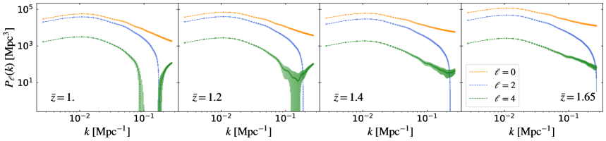
Figure 1: Galaxy clustering power spectrum Legendre multipoles, $P_{\ell}(k)$, as expected from the spectroscopic-survey data within four redshift bins (see values at Table 4). The plots show the monopole ($\ell=0$, dark red dots), quadrupole ($\ell=2$, blue dots), and hexadecapole ($\ell=4$, green dots), together with their error bars as given by the corresponding Gaussian covariance matrix. The Poissonian shot noise has been subtracted from the monopole for clarity of plotting.

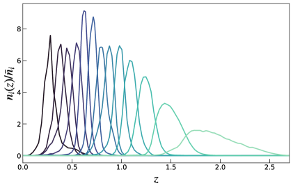
Figure 2: Normalised equi-populated photometric galaxy redshift distributions, $n_{i}(z)/\bar{n}_{i}$, corresponding to DR3.

As described in Sect. 3.3, we generate synthetic data vectors for the power spectrum Legendre multipoles $P_{\ell}(k)$ adopting the EFTofLSS framework. Our reference setup consists of four spectroscopic bins across the redshift range $0.9\leq z\leq 1.8$, and the $P_{\ell}(k)$ are generated at the mean redshift of each bin, corresponding to the values $\bar{z}_{i}=\{1.0,1.2,1.4,1.65\}$. The multipoles are then sampled over 75 linearly-spaced $k$ bins from $k_{\rm min}=0.004\,\,h\,{\rm Mpc}^{-1}$ to $k_{\rm max}=0.3\,\,h\,{\rm Mpc}^{-1}$. In all cases, we consider only the first three even terms of the multipole expansion, i.e. $\ell\in\{0,2,4\}$.

The reference values of the cosmological parameters and the ones of the EFTofLSS expansion in each spectroscopic bin are listed in Table 2. The latter has been calibrated from a synthetic model for the luminosity function of H$\alpha$ emitters (Model 3 in Pozzetti et al. 2016) as implemented in the Flagship Simulation 1, which is a previous en-suite simulation developed before the Flagship Simulation 2 (Euclid Collaboration: Castander et al. 2025). We do not include Alcock–Paczynski (AP) parameters in the computation of the spectroscopic synthetic data vectors, as we computed the synthetic data vectors on the same fiducial cosmology. See Paper 1 for the definition of the AP parameters.

We plot the resultant data vectors in Fig. 1. In all cases, the Poissonian shot noise, defined as the inverse of the target number density in the specific redshift bin, $P_{\rm SN}=1/\bar{N}$, has been subtracted from the monopole $P_{0}(k)$. We do this to minimise the impact of the lower number density of detectable H$\alpha$ galaxies, as shown in the corresponding rows of Table 4. At the same time, the overall amplitude of the monopole is similarly influenced by the excess of non-Poissonian shot noise, which is determined by the parameters $\alpha_{\rm P}$. Also in this case, high-redshift snapshots exhibit a larger value of this parameter (see Table 2), hence the larger relative importance of shot noise at small scales.

In terms of observational systematics, we model the impact of catastrophic outliers in the observed spectroscopic H$\alpha$ sample with a scale-independent damping factor to the anisotropic galaxy power spectrum. This recipe assumes that line (S [iii] and O [iii]) and noise interlopers do not cluster among themselves and with the underlying H$\alpha$ population. For a more realistic analysis, such as the one that will be realised with Euclid data, the presence of interlopers will be accounted for either at the level of the power spectrum estimator or in the modelling (Euclid Collaboration: Risso et al. 2025). The reference values for the fraction of H$\alpha$ emitters, line, and noise interlopers, as estimated from dedicated end-to-end simulations, are listed in Table 4.

Finally, the effect of spectroscopic redshift uncertainties manifests itself in the damping of the small-scale galaxy power spectrum, which is caused by the smearing of the galaxy density field along the line of sight. This is included in the synthetic data vectors, assuming a Gaussian damping with $\sigma_{z}=0.002$.

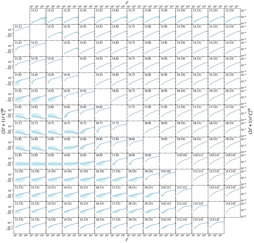
Figure 3: Synthetic harmonic-space weak lensing, $C_{ij}^{EE}(\ell)$ (upper triangle) and angular clustering power spectra, $C_{ij}^{gg}(\ell)$ (lower triangle), for the auto and cross-correlations between the 13 photometric redshift bins. The shaded error bars show the corresponding uncertainty given by the corresponding analytical covariance matrix. We have used the $C_{\ell}$ notation in the axis labels, as here they refer to the discrete measured power spectra at binned ranges of $\ell$’s.

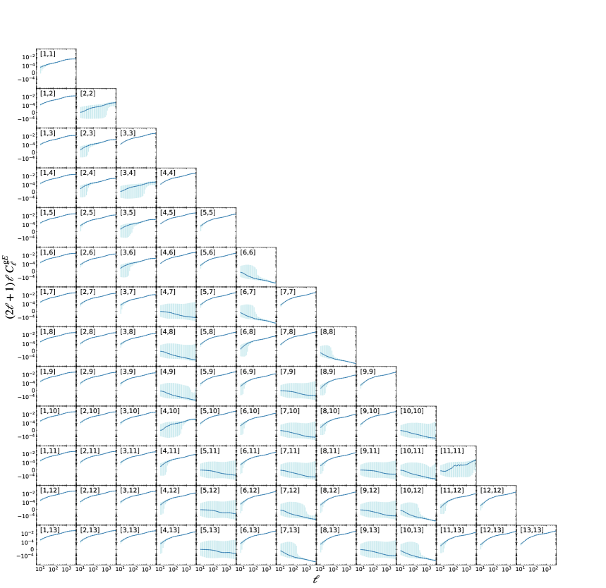
Figure 4: Similar to Fig. 3 but showing the cross-correlation galaxy-galaxy lensing XC probe $C_{ij}^{gE}(\ell)$.

5 Covariance matrices

In this section, we describe the modelling of the covariance matrices for both photometric and spectroscopic probes. Potential cross-covariances between these observables are not included, as they have been shown to be negligible (Taylor & Markovič 2022; Euclid Collaboration: Paganin et al. 2024).

5.1 Covariance for photometric observables

In this work, we follow an analytical prescription to model the harmonic-space covariance matrix, which is composed of both Gaussian and non-Gaussian contributions.

The former corresponds to the covariance of a Gaussian-distributed random field, while the latter arises due to the coupling of the Fourier modes of the density field caused by small scale non-linear evolution. Labelling the modes with wavelengths shorter (larger) than the linear survey size as sub- (super-) survey, we can divide the non-Gaussian covariance into super-sample covariance (SSC; Takada & Hu 2013), arising from sub- to super-survey mode coupling, and connected non-Gaussian covariance, arising from sub- to sub-survey mode coupling (Scoccimarro et al. 1999).

In the present work, we only account for the super-sample covariance term, since the connected non-Gaussian term has been suggested to be subdominant in Barreira et al. (2018). We have also ignored the off-diagonal terms induced by survey shape and masking, and accounted for survey shape in both the Gaussian and SSC terms by rescaling the covariance matrices by the appropriate $f_{\rm{sky}}$ (Knox 1997). The analytical expression for the Gaussian covariance is given by (see e.g. Euclid Collaboration: Blanchard et al. 2020)

$$\vskip-100.0pt{\rm Cov_{\rm G}} \left[C_{ij}^{AB}(\ell),C_{kl}^{CD}(\ell^{\prime})\right]=\left[(2\,\ell+1)\,f_{\rm sky}\,\varDelta\ell\right]^{-1}\delta_{\ell\ell^{\prime}}^{\rm K}$$

$$\times\Bigg\{\left[C_{ik}^{AC}(\ell)+{N}_{ik}^{AC}(\ell)\right]\left[C_{jl}^{BD}(\ell^{\prime})+N_{jl}^{BD}(\ell^{\prime})\right]$$

$$+\left[C_{il}^{AD}(\ell)+N_{il}^{AD}(\ell)\right]\left[C_{jk}^{BC}(\ell^{\prime})+N_{jk}^{BC}(\ell^{\prime})\right]\Bigg\}\;,$$ (15)

where the noise power spectra $N_{ij}^{AB}(\ell)$ for the different probe combinations are

$$N_{ij}^{AB}(\ell)=\left\{\begin{array}[]{ll}\displaystyle{(\sigma_{\epsilon}^{2}/2\bar{n}_{i}^{\rm L})\,\delta_{ij}^{\rm K}}&\displaystyle{A=B={\rm L}\;\;({\rm WL})}\\ &\\ \displaystyle{0}&\displaystyle{A\neq B}\\ &\\ \displaystyle{(1/\bar{n}_{i}^{\rm G})\,\delta_{ij}^{\rm K}}&\displaystyle{A=B={\rm G}\;\;({\rm GCph}})\\ \end{array}\right.\;.$$ (16)

In the above equations, the Kronecker delta symbols $\delta^{\rm K}$ enforce the absence of cross-multipole covariance and of cross-bin noise. The term $\sigma_{\epsilon}^{2}$ accounts for the total intrinsic ellipticity dispersion of the sources, with $\sigma_{\epsilon}=\sqrt{2}\,\sigma_{\epsilon}^{(i)}$, $\sigma_{\epsilon}^{(i)}$ being the ellipticity dispersion per component of the galaxy ellipticity. Finally, $\bar{n}_{i}^{A}$ is the average density of objects for weak lensing (L) and photometric galaxy clustering (G) in the $i$th redshift bin, while $\varDelta\ell$ is the width of the multipole bin centred on a given $\ell$. This expression accounts for the finite survey volume via a rescaling by the fraction of the total sky area covered by the survey, $f_{\rm sky}$, which is expected to be sufficiently accurate for large survey areas.

As for SSC, we follow the modelling of Takada & Hu (2013), adapted to the multi-probe case in Krause & Eifler (2017) and used to forecast the SSC impact in Euclid Collaboration: Sciotti et al. (2024)

$${\rm Cov_{SSC}}\left[C_{ij}^{AB}(\ell),C_{kl}^{CD}(\ell^{\prime})\right]\simeq\frac{1}{f_{\rm sky}}\int{\rm d}V_{1}{\rm d}V_{2}\;W^{A}_{i}(z_{1})\,W^{B}_{j}(z_{1})\,\\ \times W^{C}_{k}(z_{2})\,W^{D}_{l}(z_{2})\frac{\partial P_{AB}(k_{\ell};z_{1})}{\partial\delta_{\rm b}}\,\frac{\partial P_{CD}(k_{\ell}^{\prime};z_{2})}{\partial\delta_{\rm b}}\,\sigma^{2}(z_{1},z_{2})\;.$$ (17)

In the expression above, the two main ingredients needed for SSC appear. The former, called probe response, is the derivative of the cross-spectrum $P_{AB}$ between probes $A$ and $B$ with respect to a change in the background density $\delta_{\rm b}$ induced by super-survey modes. The latter is the covariance of $\delta_{\rm b}$, given by the linear power spectrum as these modes are in the linear regime, i.e.

$$\sigma^{2}(z_{1},z_{2})=\frac{1}{2\pi^{2}}\int{\rm d}k\;k^{2}\,P_{\rm mm}^{\,\rm lin}\left(k,z_{12}\right)\,{\rm j}_{0}\left(kr_{1}\right)\,{\rm j}_{0}\left(kr_{2}\right)\;.$$ (18)

For this term, we follow the modelling of Lacasa & Rosenfeld (2016), which does not assume $\sigma^{2}(z_{1},z_{2}\neq z_{1})=0$ as commonly done in the literature to speed up the SSC computation; to this end, we employ a new code, Spaceborne (Euclid Collaboration: Sciotti et al. 2025). The above expression is valid for the full, curved-sky case, and the partial sky coverage is accounted for via a normalisation by $f_{\rm sky}$, which has been shown in Gouyou Beauchamps et al. (2022) to be accurate for large survey areas. Further details on the harmonic-space covariance matrix modelling and its numerical implementation using Spaceborne are given in Euclid Collaboration: Sciotti et al. (2025).

5.2 Covariance for spectroscopic observables

Table 4: Specifications for the construction of analytical covariance matrices of the spectroscopic galaxy power spectrum Legendre multipoles.

Parameter	bin 1	bin 2	bin 3	bin 4
$\bar{z}$	1.0	1.2	1.4	1.65
redshift range	[0.9, 1.1]	[1.1, 1.3]	[1.3, 1.5]	[1.5, 1.8]
$V_{\rm shell}\,[\,h^{-3}\,{\rm Gpc^{3}}]$	$7.03$	$8.10$	$8.90$	$14.36$
$f^{\,\rm P}_{\rm[H\alpha]}$	$0.805$	$0.796$	$0.694$	$0.879$
$f^{\,\rm P}_{\rm S\,[{\textsc{iii}}]}$	$0.021$	$0.028$	$0.101$	$0.049$
$f^{\,\rm P}_{\rm O\,[{\textsc{iii}}]}$	$0.029$	$0.109$	$0.118$	$0.020$
$f^{\,\rm P}_{\rm noise}$	$0.145$	$0.067$	$0.087$	$0.052$
$f^{\,\rm C}_{\rm[H\alpha]}$	$0.387$	$0.638$	$0.724$	$0.997$
$f^{\,\rm C}_{\rm S\,[{\textsc{iii}}]}$	$0.010$	$0.022$	$0.105$	$0.056$
$f^{\,\rm C}_{\rm O\,[{\textsc{iii}}]}$	$0.014$	$0.088$	$0.123$	$0.023$
$f^{\,\rm C}_{\rm noise}$	$0.070$	$0.054$	$0.091$	$0.059$
$\bar{n}_{\rm true}\,[h^{3}\,{\rm Mpc}^{-3}]$	$14.28\,10^{-4}$	$9.49\,10^{-4}$	$6.44\,10^{-4}$	$4.03\,10^{-4}$
$\bar{n}_{\rm meas}\,[h^{3}\,{\rm Mpc}^{-3}]$	$6.87\,10^{-4}$	$7.61\,10^{-4}$	$6.71\,10^{-4}$	$4.57\,10^{-4}$

Note: Different columns show the left and right edge of the selected redshift bin, the shell volume measured according to the fiducial cosmology, the purity and completeness fractions of H$\alpha$ galaxies, S [iii] and O [iii]line interlopers, and noise interlopers, the true and measured number density of H$\alpha$ galaxies.

For spectroscopic galaxy clustering, as mentioned in Sect. 4.2, we assume four redshift bins with the same geometric specifications adopted in Euclid Collaboration: Blanchard et al. (2020). This corresponds to the nominal final-mission angular footprint of $13\,245\,\mathrm{deg}^{2}$ and four spectroscopic bins spanning $z\in[0.9,1.8]$, as shown in Table 4. We determine the covariance matrix for the power spectrum multipoles within the Gaussian approximation, following the procedure detailed in Grieb et al. (2016). The per-mode covariance of each multipole combination $\ell=\{0,2,4\}$ can be defined as

$$\begin{split}\sigma^{2}_{\ell_{1}\ell_{2}}(k\,|\,z)=\;&\frac{(2\ell_{1}+1)\,(2\ell_{2}+1)}{V_{\rm shell}}\\ &\times\int_{-1}^{\,1}\left[P_{\rm gg}(k,\mu\,|\,z)+\frac{1}{\bar{n}}\right]{\cal L}_{\ell_{1}}(\mu)\,{\cal L}_{\ell_{2}}(\mu)\,{\rm d}\mu\;,\end{split}$$ (19)

where $V_{\rm shell}$ and $\bar{n}$ are the volume and number density of the spectroscopic sample under consideration, and ${\cal L}_{\ell}$ is the $\ell$th-order Legendre polynomial. The bin-averaged multipole covariance can be derived from the previous expression as

$$C_{\ell_{1}\ell_{2}}(k_{i},k_{j})=\frac{2\,(2\pi)^{4}}{V_{k_{i}}^{\,2}}\,\delta^{\rm K}_{ij}\int_{k_{i}-\varDelta k/2}^{\,k_{i}+\varDelta k/2}\sigma^{2}_{\ell_{1}\ell_{2}}(k)\,k^{2}\,{\rm d}k\;,$$ (20)

where $V_{k_{i}}=4\pi/3\,\{[(k_{i}+\varDelta k/2)]^{3}-[(k_{i}-\varDelta k/2)]^{3}\}$ is the volume of a spherical shell centred at $k_{i}$ of width $\varDelta k$.

The Kronecker symbol marks the diagonal nature of the covariance matrix, under the Gaussian approximation. While this assumption is bound to break on sufficiently small scales, recent analyses (e.g., Blot et al. 2019; Wadekar et al. 2020) have proven how the statistical constraint on cosmological parameters is only marginally affected ($\lesssim 10\%$) by the presence of non-linear corrections to the multipole covariance matrix (Scoccimarro et al. 1999; Sefusatti et al. 2006; Blot et al. 2015, 2016; Bertolini et al. 2016; Wadekar & Scoccimarro 2020). We adopt this approach for deriving these forecasts, whereas a more complete model shall be adopted for future analyses, such as the one of the DR1 data.

We account for the impact of observational systematic effects on the covariance matrix by adopting the same fractions of true H$\alpha$ (with a good quality redshift or not) line, and noise interlopers as calibrated with the FastSpec simulator (Cagliari et al. 2024) using a Euclid Wide Survey configuration.

The completeness of the sample is defined as the fraction of correctly targeted H$\alpha$ galaxies to the total H$\alpha$ population, while the purity of the sample is defined as the fraction of H$\alpha$ galaxies with correct redshift to the total observed sample. In turn, the latter is expected to contain S [iii] and O [iii] contaminants due to line mis-identification, and noise interlopers due to the presence of catastrophic redshift errors. These two falsely-detected populations modify the total clustering amplitude such that the total observed number density $n_{\rm obs}(z)$ and clustering amplitude $P_{\rm obs}(k,\mu)$ differs from the true quantities $n_{\rm true}(z)$ and $P_{\rm true}(k,\mu)$, as

$$n_{\rm obs}(z)=n_{\rm true}(z)\,\frac{1-f_{\rm inc}}{1-f_{\rm out}}\;,$$ (21)

and

$$P_{\rm obs}(k,\mu)=(1-f_{\rm out})^{2}\,P_{\rm true}(k,\mu)\;.$$ (22)

In the above equations, $f_{\rm inc}$ and $f_{\rm out}$ represent the fraction of undetected and falsely detected H$\alpha$ galaxies respectively. The observed number density and galaxy power spectrum are the quantities that are ultimately used in Eq. 19 to obtain the per-mode covariance of the power spectrum multipoles.

6 Forecast results

Table 5: $\mathrm{FoM}$ for the dark energy parameters $w_{0}$ and $w_{a}$ given different cosmological models and Euclid probes.

Cosmological model	WL	GCsp	3×2pt	3×2pt + GCsp
$w_{0}w_{a}\mathrm{CDM}$ (flat)	21	35	380	500
$w_{0}w_{a}\mathrm{CDM}$ (non-flat)	11	13	186	331
$w_{0}w_{a}\mathrm{CDM}$ + $\gamma_{\mathrm{g}}$ (flat)	9	24	243	327

Note: The $w_{0}$ and $w_{a}$ two-dimensional posterior contours can be seen in Fig. 6 for Weak Lensing (WL), in Fig. 8 for Spectroscopic Galaxy Clustering (GCsp), in Fig. 9 for the photometric combination probe weak lensing, angular clustering and galaxy-galaxy lensing (3×2pt), and in Fig. 14 for the combination of 3×2pt and GCsp.

Table 6: 68% confidence limits for the cosmological nuisance parameters in the $w_{0}w_{a}\mathrm{CDM}$ model, assuming a flat geometry.

	WL	GCsp	3×2pt	3×2pt + GCsp
$\ln{(10^{10}\,A_{\rm s})}$	$3.02^{+0.11}_{-0.13}$	$3.007\pm 0.061$	$3.039\pm 0.020$	$3.041\pm 0.013$
$n_{\rm s}$	$0.957^{+0.044}_{-0.059}$	$0.960^{+0.018}_{-0.016}$	$0.9656^{+0.0069}_{-0.0061}$	$0.9662\pm 0.0037$
$\varOmega_{{\rm b}}\,h^{2}$	$0.02269\pm 0.00036$	$0.02269\pm 0.00032$	$0.02271\pm 0.00027$	$0.02268\pm 0.00019$
$\varOmega_{{\rm c}}\,h^{2}$	$0.125^{+0.014}_{-0.016}$	$0.1230^{+0.0028}_{-0.0032}$	$0.1221^{+0.0019}_{-0.0022}$	$0.12181\pm 0.00097$
$w_{0}$	$-0.98\pm 0.20$	$-0.92^{+0.19}_{-0.25}$	$-1.003\pm 0.051$	$-1.004\pm 0.046$
$w_{a}$	$-0.10^{+0.68}_{-0.47}$	$-0.28^{+0.74}_{-0.50}$	$0.01\pm 0.16$	$0.01\pm 0.13$
$S_{8}$	$0.842\pm 0.010$	$0.838\pm 0.019$	$0.8421\pm 0.0026$	$0.8419\pm 0.0024$
$\varOmega_{\rm b}$	$0.0495^{+0.0050}_{-0.0070}$	$0.0507^{+0.0033}_{-0.0039}$	$0.0499\pm 0.0011$	$0.04993\pm 0.00080$
$\varOmega_{\rm m}$	$0.321^{+0.018}_{-0.021}$	$0.327^{+0.021}_{-0.028}$	$0.3196\pm 0.0045$	$0.3195\pm 0.0043$
$\sigma_{8}$	$0.815^{+0.019}_{-0.017}$	$0.804^{+0.028}_{-0.025}$	$0.8158\pm 0.0039$	$0.8159\pm 0.0036$
$h$	$0.681\pm 0.040$	$0.671\pm 0.024$	$0.6746\pm 0.0073$	$0.6740\pm 0.0050$

Note: The table shows both constraints on sampled and derived parameters.

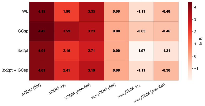
Figure 5: Heatmap of the logarithm of the Bayes factors ($\ln B$) for different cosmological models relative to $w_{0}w_{a}\mathrm{CDM}$ (flat), across various probes: Weak Lensing (WL), Galaxy Clustering (GCsp), 3$\times$2pt, and their combination. Darker red shades indicate models strongly disfavoured by the data relative to the reference, while lighter shades indicate models more compatible with the data. The Bayes factor quantifies the relative evidence for each model, automatically penalising unnecessary complexity. Overall, the data generally favour simpler $\Lambda\mathrm{CDM}$ models over extensions such as $w_{0}w_{a}\mathrm{CDM}$ or models including $\gamma_{g}$ or curvature. $\ln{\cal Z}(\boldsymbol{d}\,|\,M)$ values are found in Table 7.

We present now the main forecast results for all of Euclid’s primary probes (WL, 3×2pt, GCsp, and 3×2pt + GCsp) across six different cosmological models, assuming Euclid specifications for DR3 (Euclid Collaboration: Mellier et al. 2025), which corresponds to the nominal mission duration. The parameter space explored in this analysis, accounting for 13 tomographic bins for the photometric probes and 4 spectroscopic bins for GCsp, along with the inclusion of additional systematic nuisance parameters for each bin, ranges from 21 to 61 sampled parameters. The prior used for each cosmological and nuisance parameter is listed in Table 2. In total, we analysed 24 different cases. For each case, we also compute derived parameters from sampled parameters such as $\sigma_{8}$ and $S_{8}$ using CAMB or Eq. 9, respectively, as well as the nuisance parameters specified in Table 2.

Details of each run, including the size of the parameter space, allocated computational resources, and computational time, are listed in Appendix A, specifically in Table 7.

Recent studies in the LSS community have emphasised the impact of prior volume effects on the statistical inference of cosmological parameters (see, e.g. Carrilho et al. 2023; Hadzhiyska et al. 2023, for applications to spectroscopic and photometric probes, respectively). Specifically, the priors imposed on certain nuisance parameters – typically marginalised over – can influence the marginal posterior distributions of cosmological parameters, making these priors effectively informative. This is particularly relevant for the RSD counter-terms within the EFTofLSS framework.

To address this, we apply external information from Big Bang Nucleosynthesis (BBN) in the form of a Gaussian prior on the baryon density parameter $\varOmega_{{\rm b}}\,h^{2}$ (Cooke et al. 2018; Schöneberg et al. 2022; Schöneberg 2024) in all configurations involving GCsp. For consistency, this prior is used across all probes in the reference setup for the exploration of all the models in 6. Furthermore, we marginalise only over a limited set of nuisance parameters: $b_{\rm G}^{1}$, $b_{\rm G}^{2}$, $\alpha_{\rm P}$, and $f_{\rm out}$. We fixed the two non-local bias parameters, $b_{{\rm G}_{2}}$ and $b_{\varGamma_{3}}$, according to coevolution relations (Euclid Collaboration: Pezzotta et al. 2024). For the remaining nuisance parameters, we adopt an optimistic setup by fixing them to the fiducial values used to generate the data vectors (see third column from left of Table 2). While this approach may seem overly optimistic, we argue that with DR3, some EFTofLSS counter-terms could be constrained robustly using realistic cosmological simulations exploring diverse galaxy population models. A more comprehensive exploration of prior volume effects, incorporating all EFTofLSS nuisance parameters, will be detailed in future work (Euclid Collaboration: Moretti et al. in prep.).

Given the staggering quantity of results generated, we focus on presenting only the key highlights in this section to ensure clarity and conciseness. This approach allows us to streamline the discussion while still providing access to the full breadth of information for in-depth analysis. In all posterior distribution contour plots, the fiducial values are indicated by dashed grey lines. As part of our validation process, we conducted a series of sanity checks to ensure the robustness of our results. The samplers were carefully tested to confirm that they correctly recover the maximum of the likelihood at the fiducial model values, which were used for the generation of the synthetic data vectors. Additionally, we verified that the posterior distribution is properly sampled by employing a sufficiently large number of live points (see Sect. 2 for details), and ensured that the parameter priors are sufficiently broad to avoid hitting the boundaries during the sampling process. To reach convergence, a total number from $\mathcal{O}(10^{5})$ up to $\mathcal{O}(10^{7})$ likelihood evaluations is requested, for single probes (WL, GCsp, 3×2pt) and joint ones (3×2pt + GCsp), respectively.

For all the cases in which we explore an evolving dark energy equation of state (flat and non-flat $w_{0}w_{a}\mathrm{CDM}$, and flat $w_{0}w_{a}\mathrm{CDM}$ + $\gamma_{\mathrm{g}}$), we apply a logical prior on the $w_{0}$ $-$$w_{a}$ parameter space to avoid exploring a dark energy fluid that would not lead to an accelerated expansion in the post-inflationary epoch ($a\ll 1$), also known as the strong energy condition (Chevalier & Polarski 2001; Linder 2003),

$$w_{0}+w_{a}\leq-1/3\;.$$ (23)

This choice also enables more efficient sampling of the parameter space, as it is imposed in the analysis through an external likelihood. The final goal of the analysis is then to calculate the dark energy $\mathrm{FoM}$ for the various configurations that we explore. The obtained values are presented in Table 5. When comparing our results to those of Euclid Collaboration: Blanchard et al. (2020), we note that (1) the theoretical predictions in this paper are based on a more complex implementation than those used in Euclid Collaboration: Blanchard et al. (2020, see Paper 1 for details), and (2) we sample the full posterior distribution of the parameters of interest (Eq. 5), rather than using the Fisher formalism for forecasting as outlined in Eq. 4. The statistical best-fits and 68% confidence intervals for both sampled and derived cosmological parameters for the $w_{0}w_{a}\mathrm{CDM}$ model, following a flat geometry, are found in Table 6.

Finally, benefiting from the nested sampling algorithm, we quote the Bayes factor values using $w_{0}w_{a}$CDM (flat) as the reference model. The Bayes factor, defined as

$$B_{i,\rm ref}=\frac{\mathcal{Z}_{i}}{\mathcal{Z}_{\rm ref}}=\frac{P(D\mid M_{i})}{P(D\mid M_{\rm ref})}=\exp{\varDelta\ln{\cal Z}(\boldsymbol{d}\,|\,M)},$$ (24)

quantifies the relative evidence for model $M_{i}$ compared to the reference model $M_{\rm ref}$, taking into account both the fit to the data $d$ and the model complexity (i.e. number of parameters). In terms of Bayes factors, a difference of $\varDelta\ln{\cal Z}(\boldsymbol{d}\,|\,M)\sim 2.0$ corresponds to a Bayes factor of $B\sim e^{2}\approx 7$, which is generally considered worth mentioning. A stronger difference of $\varDelta\ln{\cal Z}(\boldsymbol{d}\,|\,M)\sim 5.0$ translates into $B\sim e^{5}\approx 150$, which falls into the “decisive” category according to Jeffreys’ scale. Across all probesWL, GCsp, 3$\times$2pt, and their combinationthe results consistently favour simpler $\Lambda\mathrm{CDM}$ models. Models including additional parameters, such as curvature or the growth modification $\gamma_{g}$, are generally penalised, with Bayes factors below unity, indicating that the data do not require these extensions. This hierarchical comparison highlights the constraining power of each probe individually and in combination, emphasising that while some extended models remain marginally allowed, the evidence strongly prefers the minimal $\Lambda\mathrm{CDM}$ framework (see Fig. 5).

6.1 Weak Lensing

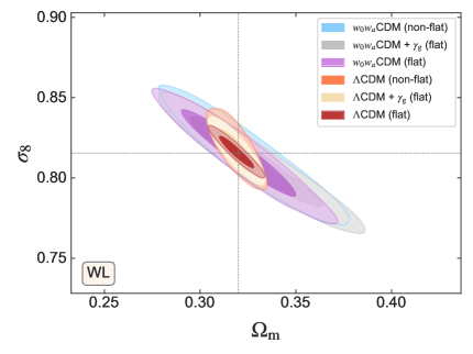
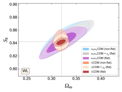
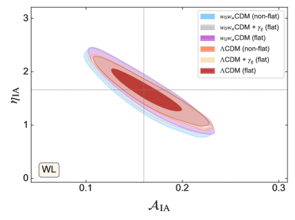
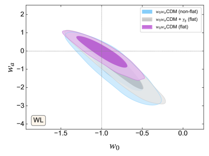
Figure 6: Two-dimensional posterior distributions for the cosmological parameters $\varOmega_{{\rm m}}$, $\sigma_{8}$ and $S_{8}$, the eNLA Intrinsic Alignment parameters $\mathcal{A}_{\mathrm{IA}}$ and $\eta_{\mathrm{IA}}$, and the dark energy parameters $w_{0}$ and $w_{a}$, using only the Weak Lensing probe (WL) for the six cosmological models. The values for the $\mathrm{FoM}$ of $w_{0}$ and $w_{a}$ can be found in Table 5.

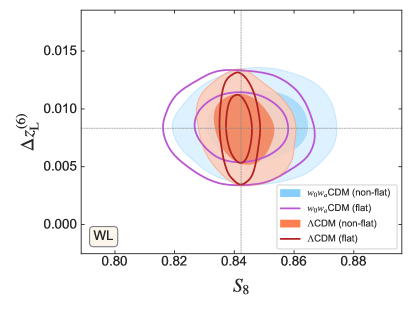
Figure 7: Two-dimensional posterior distributions for the cosmological parameter $S_{8}$ and the per-bin redshift shift nuisance parameter $\varDelta z_{\rm L}^{(6)}$, using only the Weak Lensing probe for 4 different cosmological models. The correlation between $S_{8}$ and $\varDelta z_{\rm L}^{(6)}$ is about $-0.1$ in $\Lambda\mathrm{CDM}$, while it is close to zero in the $w_{0}w_{a}\mathrm{CDM}$ model. Similar behaviour is found for $\varDelta z_{\rm L}^{(i)}$ vs. $S_{8}$ regardless of the redshift bin $i$.

Cosmic shear is a powerful probe for constraining the combination of the total matter density, $\varOmega_{{\rm m}}$, and the amplitude of matter fluctuations, $\sigma_{8}$. However, due to the strong degeneracy between these two parameters in cosmic shear measurements, weak lensing is particularly sensitive to their combination, $S_{8}$ (as defined in Eq. 9), which is better constrained and more robustly measured in this context. In Fig. 6, we present the two-dimensional sampled posterior distributions for these parameters, as well as for the dark energy parameters, $w_{0}$ and $w_{a}$, and the intrinsic alignment parameters, $\mathcal{A}_{\mathrm{IA}}$ and $\eta_{\mathrm{IA}}$. Beyond $\Lambda\mathrm{CDM}$ models, these posteriors exhibit non-Gaussian behaviour and mild prior volume effects (see Sect. 6.3.3 for detailed examples of projection effects in photometric probes). In these two-dimensional posteriors, we observe a subtle rotation in the correlation between $\sigma_{8}$ and $\varOmega_{{\rm m}}$, as well as between $S_{8}$ and $\varOmega_{{\rm m}}$, for the non-flat $\Lambda\mathrm{CDM}$ and $\Lambda\mathrm{CDM}$ + $\gamma_{G}$ models compared to the others. This rotation arises from the additional redshift freedom introduced by the parameters $w_{0}$ and $w_{a}$, which induce parameter correlations between $S_{8}$ and the per-bin redshift shifts, $\varDelta z_{\rm L}^{i}$ (see Fig. 7). As expected, the spectral index $n_{\rm s}$ cannot be constrained using the cosmic shear probe alone, since the recovered posterior distribution remains uninformative and essentially mirrors the uniform prior assumed for this parameter. Additionally, this probe fails to constrain non-flat cosmologies, since the marginalised posterior distribution of $\varOmega_{K}$ is mostly prior-dependent. As expected, we do not observe the usual degeneracies between the Hubble parameter $H_{0}$ and the baryon density $\varOmega_{{\rm b}}$ (see Doux et al. 2022, for instance) due to the inclusion of the BBN prior in the analysis.

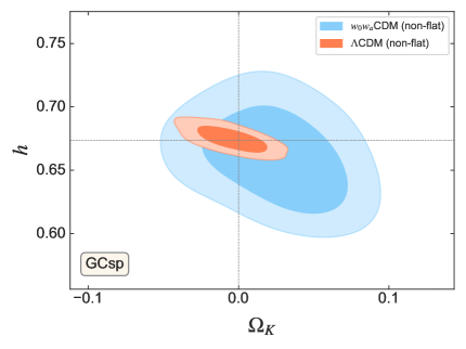
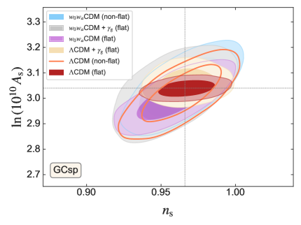
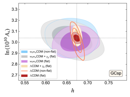
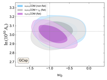
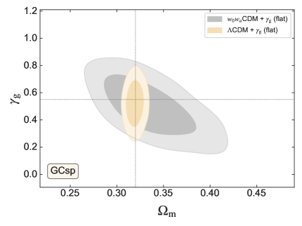
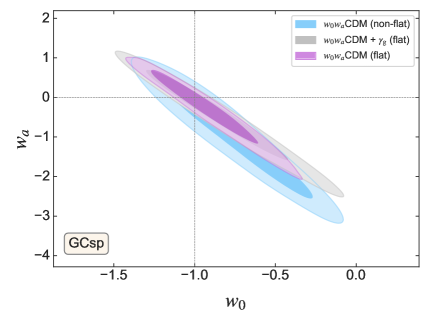
Figure 8: Two-dimensional posterior distributions for the cosmological parameters $\varOmega_{K}$, $h$, the primordial parameters $n_{\rm s}$ and $\ln(10^{10}A_{\rm s})$, $h$ and $\ln(10^{10}A_{\rm s})$, the dark energy parameter $w_{0}$ and $\ln(10^{10}A_{\rm s})$, the modified-gravity Linder parameter $\gamma_{\mathrm{g}}$, and the dark energy parameters $w_{0}$ and $w_{a}$, using only the spectroscopic galaxy clustering probe (GCsp), for the six cosmological models. The values for the $\mathrm{FoM}$ of $w_{0}$ and $w_{a}$ can be found in Table 5.

The constraining power on the dark energy parameters $w_{0}$ and $w_{a}$ is limited, with the corresponding posterior distributions displaying strongly non-Gaussian behaviour (see Fig. 6, lower right panel). The $\mathrm{FoM}$ values obtained for $w_{0}$ and $w_{a}$ using this probe (Table 5, first column) are consistent with those reported in Euclid Collaboration: Blanchard et al. (2020). Specifically, our forecasts align with the predictions for the pessimistic scenario presented in their paper, despite using a higher value for the maximum multipole ($\ell_{\rm max}$) in our analysis. This likely occurs because we employ a more sophisticated modelling approach for the cosmic shear probe in this work, including the sampling of multiplicative bias and redshift-bin shifts as systematic nuisance parameters. This increases the size of the parameter space, thereby widening our constraints.

The posterior distributions of the systematic nuisance parameters, such as the redshift bin shifts and multiplicative bias parameters, are well constrained. Most of the posteriors are either informative or prior dominated, and they remain consistent with the fiducial values (see detailed discussion in Sect. 6.3.2). In particular, by examining the full posterior distributions shown in Appendix B, Figs. 17 and 18 for the redshift shifts and multiplicative biases, we conclude that these parameters are prior dominated. This is expected, as the priors adopted reflect the Euclid science requirements for the primary photometric probe – $3\times 2$pt – which are more stringent than for shear-only analyses.

Specifically, the results in Fig. 6 (lower left panel) demonstrate that the constraints on the intrinsic alignment parameters in the eNLA model are cosmological model-independent, with no significant differences in the constraints across the six models studied. This indicates that $\mathcal{A}_{\mathrm{IA}}$ and $\eta_{\mathrm{IA}}$ are not degenerate with the dark energy parameters $w_{0}$ and $w_{a}$, or with the modified gravity parameter $\gamma_{\mathrm{g}}$, and that they are independent of cosmological geometry. This is due to the definition of the IA model in the theoretical prescription of the cosmic shear probe (see Paper 1, Eq. 116), where the IA parameters contribute both linearly and quadratically to the cosmic-shear power spectrum. We also show the correlation matrices between the intrinsic alignment parameters, and $\varOmega_{{\rm m}}$ and $S_{8}$ to investigate further degeneracies. The correlations among the four key parameters $\mathcal{A}_{\mathrm{IA}}$, $\eta_{\mathrm{IA}}$, $\varOmega_{{\rm m}}$, and $S_{8}$ exhibit similar qualitative behaviour in both $\Lambda\mathrm{CDM}$ and $w_{0}w_{a}\mathrm{CDM}$ models. In particular, the matter density $\varOmega_{{\rm m}}$ and the clustering amplitude parameter $S_{8}$ continue to show a positive correlation, reflecting their joint influence on structure growth. However, the introduction of the dark energy parameters in the $w_{0}w_{a}\mathrm{CDM}$ introduces additional degeneracies that mildly affect the strength of these correlations. This results in a slight broadening of parameter degeneracies.

Finally, we note that our results show a rotation in the direction of degeneracy between $\sigma_{8}$ and $\varOmega_{{\rm m}}$ as compared to $S_{8}$ and $\varOmega_{{\rm m}}$ in the two-dimensional posteriors, relative to previous Stage-III results (e.g. Abbott et al. 2022, which shows the same direction of degeneracy in both the $\sigma_{8}$-$\varOmega_{{\rm m}}$ and the $S_{8}$-$\varOmega_{{\rm m}}$ plane). We investigated this rotation and found that it results from using a BBN prior and the increased constraining power of this probe for Euclid-like surveys.

For Euclid DR3, we anticipate an improvement by one order of magnitude over previous surveys in constraining $\sigma_{8}$ and $S_{8}$ for $\Lambda\mathrm{CDM}$ KiDS-1000 legacy survey (Wright et al. 2025) and DES Y3 (Doux et al. 2022):

Euclid $$\sigma_{8}=0.816^{+0.013}_{-0.013},\quad S_{8}=0.8416^{+0.0056}_{-0.0052}.$$

DES Y3 $$\sigma_{8}=0.863\pm 0.096,\quad S_{8}=0.793^{+0.038}_{-0.025}.$$

KiDS legacy $$S_{8}=0.815^{+0.016}_{-0.020}.$$

Euclid achieves an improvement of one order of magnitude in $S_{8}$, with a precision of $\sigma(S_{8})=0.0054$, compared to $\sigma(S_{8})\approx 0.0315$ from DES Y3 and $\sigma(S_{8})\approx 0.018$ from KiDS-1000. This corresponds to an improvement of approximately $83\%$ relative to DES Y3 and $70\%$ relative to KiDS-1000.

6.2 Spectroscopic galaxy clustering

The large-scale distribution of galaxies can be used to effectively put constraints on cosmological parameters via the growth of cosmic structures (through RSD) and the geometrical information (through the Alcock-Paczynski cosmological test). In Fig. 8, we show the two-dimensional sampled posterior distributions for $H_{0}$, $\varOmega_{{\rm m}}$, $\varOmega_{K}$, the primordial parameters $n_{\rm s}$ and $\ln(10^{10}A_{\rm s})$, the modified gravity parameter $\gamma_{\mathrm{g}}$, as well as the dark energy parameters $w_{0}$ and $w_{a}$ for the spectroscopic galaxy clustering (GCsp) probe. Overall, in beyond-$\Lambda\mathrm{CDM}$ (flat) model extensions, the posterior distributions are strongly non-Gaussian and show projection effects.

Contrary to cosmic shear-only, we observe that spectroscopic galaxy clustering is able to constrain the primordial parameter $\ln(10^{10}A_{\rm s})$ significantly. The constraint on $n_{\rm s}$ arises primarily because the majority of the nuisance parameters are fixed, and high GCph scale cuts are assumed. In the absence of these conditions, $n_{\rm s}$ exhibits significant degeneracy with the nuisance parameters. For more details, we refer the reader to the future work of Euclid Collaboration: Moretti et al. (in prep.).

Interestingly, in the two-dimensional posteriors, we observe a change in the degeneracy direction between $n_{\rm s}$ and $\ln(10^{10}A_{\rm s})$ for the $w_{0}w_{a}\mathrm{CDM}$ models, as compared to flat and non-flat $\Lambda\mathrm{CDM}$ (see Fig. 8, upper right panel). This degeneracy can be explained when the two-dimensional posterior of $H_{0}$ and $\ln(10^{10}A_{\rm s})$ is illustrated (see Fig. 8, middle left panel), where the presence of the dark energy parameters $w_{0}$ and $w_{a}$ introduces extra degrees of freedom and broader contours for $\ln(10^{10}A_{\rm s})$ (see Fig. 8, middle right panel).

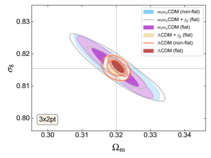
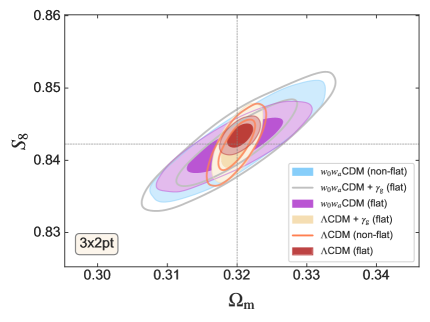
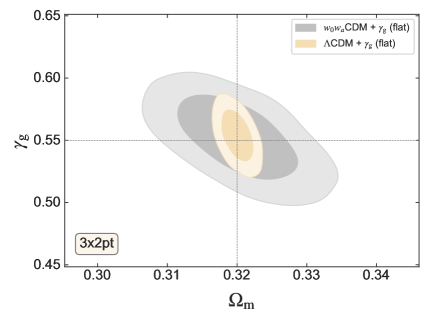
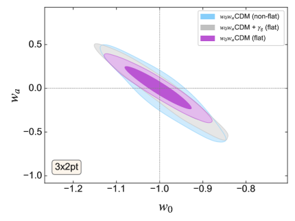
Figure 9: Two-dimensional posterior distributions for the cosmological parameters $\varOmega_{{\rm m}}$, $\sigma_{8}$ and $S_{8}$, $w_{0}$ and $w_{a}$, and $\varOmega_{{\rm m}}$ and $\gamma_{\mathrm{g}}$, using the full photometric probe combination 3×2pt. The values for the $\mathrm{FoM}$ of $w_{0}$ and $w_{a}$ can be found in Table 5.

Spectroscopic galaxy clustering alone exhibits substantially weaker constraining power on $S_{8}$ compared to cosmic shear, as expected given the sensitivity of each probe. In the context of the $\Lambda\mathrm{CDM}$ model, specifically, the relative uncertainty on $S_{8}$ from GCsp ($S_{8}=0.841^{+0.030}_{-0.029}$) is approximately 446% larger than that from WL alone ($S_{8}=0.8416^{+0.0056}_{-0.0052}$), the latter being more directly sensitive to the amplitude of matter fluctuations. Similarly to the cosmic-shear only case, the BBN priors break the degeneracy between the Hubble parameter $H_{0}$ and the baryon density $\varOmega_{{\rm b}}$.

Notably, spectroscopic galaxy clustering on its own provides significant constraints on non-flat cosmologies (Fig. 8, upper left panel). When comparing the BAO-only results from DESI Collaboration: Adame et al. (2024b) to our predictions for the full-shape analysis of spectroscopic galaxy clustering, both results are consistent, and we forecast a 50% improvement in the measurement of $\varOmega_{K}$ with Euclid only. Furthermore, we also predict that the modified gravity $\gamma_{\mathrm{g}}$ parameter (Fig. 8, lower left panel) can be constrained with full shape galaxy clustering only. In both the $\Lambda\mathrm{CDM}$ and $w_{0}w_{a}\mathrm{CDM}$ extensions, $\gamma_{\mathrm{g}}$ is measured with an uncertainty of approximately 0.2 and 0.3, respectively, indicating that it is better constrained in $\Lambda\mathrm{CDM}$. In relative terms, this corresponds to a 42% uncertainty in $\Lambda\mathrm{CDM}$ versus 57% in $w_{0}w_{a}\mathrm{CDM}$, showing that more information is gained on $\gamma_{\mathrm{g}}$ in the $\Lambda\mathrm{CDM}$ scenario. For Euclid DR3, we anticipate an improvement by one order of magnitude in general over former surveys like eBOSS (Alam et al. 2021) and first preliminary DESI results (DESI Collaboration: Adame et al. 2024b, a; DESI Collaboration et al. 2025).

The obtained $\mathrm{FoM}$ values for $w_{0}$ and $w_{a}$ using spectroscopic angular clustering (Table 5, second column) fall within the pessimistic-optimistic constraint range presented in Euclid Collaboration: Blanchard et al. (2020), aligning more closely with the predictions for the optimistic scenario. This is most likely due to the reduced parameter space sampled here, as many nuisance parameters of the theoretical modelling have been fixed to mitigate the impact of projection effects.

The posterior distributions corresponding to the systematic nuisance parameters that are freely sampled (e.g. bias, purity, and Poissonian shot noise parameters) are well-constrained and recover the fiducial values. Examples of these posterior distributions can be seen in Figs. 20 and 21. In particular, the purity parameters, although sampled from a Gaussian prior distribution, are more tightly constrained than the prior in the first redshift bin. They also exhibit correlations across the remaining redshift bins, where the posterior distributions are broader. These correlations impact the cosmological parameters as well, with non-negligible degeneracies observed with $A_{\rm s}$, $n_{\rm s}$, and $H_{0}$, especially for the purity parameters in the higher redshift bins. The strongest correlation is found between $A_{\rm s}$ and the purity parameter in the third redshift bin, with a correlation coefficient of 0.2.

6.3 3×2pt

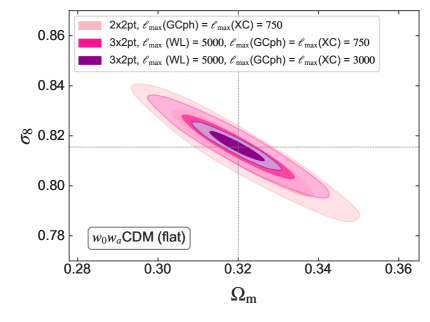
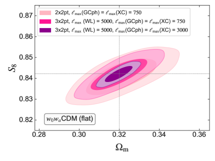
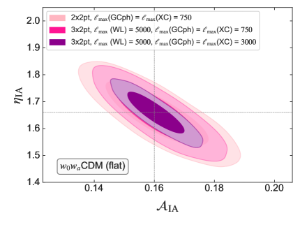
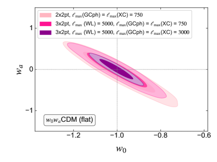
Figure 10: Two-dimensional posterior distributions for the cosmological parameters $\varOmega_{{\rm m}}$, $\sigma_{8}$ and $S_{8}$, $w_{0}$ and $w_{a}$, and $\eta_{\mathrm{IA}}$ and $\mathcal{A}_{\mathrm{IA}}$, only for the $w_{0}w_{a}\mathrm{CDM}$ model adopting a flat geometry, using the full photometric probe combination of 3×2pt, and the combination of only angular clustering and galaxy-galaxy lensing (2×2pt). The colour pattern indicates different scale cuts for angular clustering and galaxy-galaxy lensing (either $\ell_{\rm max}=$ 3000 or 750). The values for the $\mathrm{FoM}$ of $w_{0}$ and $w_{a}$ are 380 for 3×2pt ( $\ell_{\rm max}=$ 3000), 110 for 3×2pt ( $\ell_{\rm max}=$ 750) and 81 for 2×2pt.

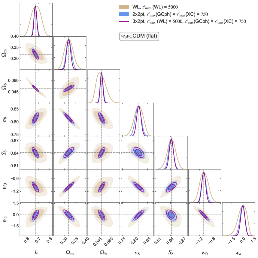
Figure 11: Forecast of the constraints for the $w_{0}w_{a}\mathrm{CDM}$ cosmological model (adopting a flat geometry) using only Euclid photometric probes: cosmic shear (WL), galaxy-galaxy lensing and angular clustering, 2×2pt, and cosmic shear, galaxy-galaxy lensing and angular clustering, 3×2pt, as described in Sect. 6.3.1. For the photometric probes, we used $\ell_{\rm max}=5000$ for cosmic shear and $\ell_{\rm max}=750$ for photometric angular clustering, and galaxy-galaxy lensing. The corresponding $\mathrm{FoM}$ obtained for each sample can be found either in Table 5 (WL) and in the text of the corresponding section (2×2pt and 3×2pt). The values for the $\mathrm{FoM}$ of $w_{0}$ and $w_{a}$ are 21 for the Weal Lensing probe (WL), 110 for 3×2pt ( $\ell_{\rm max}=$ 750) and 81 for 2×2pt.

The 3×2pt probe, which combines angular galaxy clustering (GCph), galaxy-galaxy lensing (XC) and cosmic shear (WL), is an effective tool for constraining $\varOmega_{{\rm m}}$ and $\sigma_{8}$, similarly to WL, and $w_{0}$, $w_{a}$ and $\gamma_{\mathrm{g}}$, as well as several nuisance parameters associated to the modelling of effects such as intrinsic alignment, galaxy bias, and magnification. In Fig. 9, we present the main highlights from the full posterior distributions by plotting the marginalised two-dimensional posteriors for the main parameter combination, as we did in Figs. 6 and 8. In subsequent subsections, we analyse in detail the particular behaviour of 3×2pt for different scale cuts in the $w_{0}w_{a}\mathrm{CDM}$ model adopting a flat geometry (Sect. 6.3.1). We study the impact of sampling experimental nuisance systematic parameters on the posterior distributions of the cosmological parameters (Sect. 6.3.2), and evaluate the presence of possible projection effects in the $\Lambda\mathrm{CDM}$ and $w_{0}w_{a}\mathrm{CDM}$ models also adopting a flat geometry (Sect. 6.3.3).

The expected constraints in the $\sigma_{8}$ $-$$\varOmega_{{\rm m}}$ and $S_{8}-$$\varOmega_{{\rm m}}$ planes show an improvement by one order of magnitude with respect to WL only (see Fig. 9, upper row). As in the case of both WL and GCsp, we see a difference in the direction of degeneracy between $\sigma_{8}$ and $\varOmega_{{\rm m}}$ compared to $S_{8}$ and $\varOmega_{{\rm m}}$ in the two-dimensional posteriors. Although not explicitly shown, 3×2pt also constrains the primordial parameters $n_{\rm s}$ and $\ln(10^{10}A_{\rm s})$. This joint probe is also able to constrain the Hubble parameter $H_{0}$, partially due to the extra prior information from the BBN prior, and to the incorporation of angular clustering, which breaks parameter degeneracies. Similarly to WL only, for Euclid DR3, we anticipate an improvement by one order of magnitude with respect to completed surveys in terms of constraints on $\sigma_{8}$ and $S_{8}$ (Heymans et al. 2021; Abbott et al. 2022) within the $\Lambda\mathrm{CDM}$ model:

Euclid $$\sigma_{8}=0.8161^{+0.0026}_{-0.0025},\quad S_{8}=0.8434^{+0.0022}_{-0.0021}.$$

DES Y3 $$\sigma_{8}=0.733^{+0.039}_{-0.049},\quad S_{8}=0.776\pm 0.017.$$

KiDS-1000 $$S_{8}=0.766^{+0.020}_{-0.01}.$$

Euclid achieves an improvement of one order of magnitude in $S_{8}$, with a precision of $\sigma(S_{8})\approx 0.0022$, compared to $\sigma(S_{8})\approx 0.017$ from DES Y3 and $\sigma(S_{8})\approx 0.02$ from KiDS-1000. The improvement with respect to shear-only is driven by angular photometric galaxy clustering.

The increase in the constraining power on the dark energy parameters $w_{0}$ and $w_{a}$ (see Fig. 9, lower right panel) for 3×2pt with respect to single probes is remarkable. The obtained $\mathrm{FoM}$ values for $w_{0}$ and $w_{a}$ using this probe (Table 5, third column) are consistent with those reported in Euclid Collaboration: Blanchard et al. (2020). Specifically, our forecasts align with the predictions for the pessimistic scenario, despite using high GCph scale cuts. Similarly to cosmic shear, the reason behind this is the increase in the number of sampled nuisance parameters in the analysis, which broadens the overall posterior distribution. Yet, we predict a $\mathrm{FoM}$ value of approximately 380 for the $w_{0}w_{a}\mathrm{CDM}$ (flat) model, which is one order of magnitude larger than the $\mathrm{FoM}$ calculated for single probes WL and GCsp.

The systematic nuisance parameters (e.g. shifts in the redshift bins and multiplicative bias parameters) and other physical effect parameters (intrinsic alignments, galaxy bias, magnification bias) are well-constrained given the informative priors provided by Euclid science requirements, accurately recovering the fiducial values (Figs. 17, 18 and 19). The magnification biases and redshift bin shifts remain prior-dominated, with no significant improvement from the inclusion of angular photometric galaxy clustering; see Fig. 19. These parameters show minimal correlations or degeneracies with the cosmological parameters. However, moderate degeneracies, particularly at the level of approximately 0.2, are observed between the photometric galaxy and magnification biases and certain cosmological parameters, most notably $\varOmega_{{\rm m}}$. Although not explicitly shown, similarly to the WL case, the resulting 2D-marginalised posterior distributions corresponding to the intrinsic alignment parameters in the eNLA model, $\mathcal{A}_{\mathrm{IA}}$ and $\eta_{\mathrm{IA}}$, are cosmological-model independent. The photometric galaxy bias nuisance parameters are strongly correlated, showing correlation coefficients of at least 0.9.

6.3.1 Impact of scale cuts for angular clustering and cosmic shear on 3×2pt probe

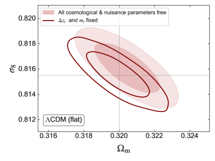
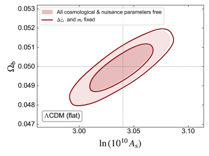
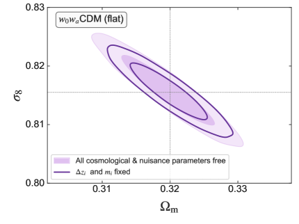
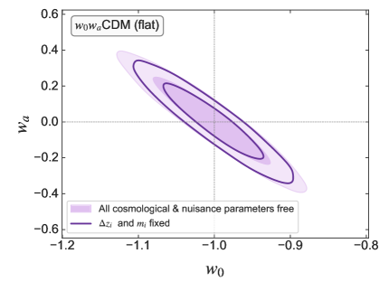
Figure 12: Two-dimensional posterior distributions for the cosmological parameters $\varOmega_{{\rm m}}$, $\sigma_{8}$, $\ln(10^{10}A_{\rm s})$, $\varOmega_{{\rm b}}$, $w_{0}$ and $w_{a}$, for the models $\Lambda\mathrm{CDM}$ and $w_{0}w_{a}\mathrm{CDM}$ adopting a flat geometry, when the systematic mean redshift-bin shifts $\varDelta z^{\rm L}_{i}$ and shear multiplicative bias $m_{i}$ nuisance parameters are sampled (filled contours) or kept fixed (unfilled contours). The variation in the values of the obtained $\mathrm{FoM}$ for the dark energy parameters can be found in the text in Sect. 6.3.2.

To understand the significant improvement in the dark energy $\mathrm{FoM}$ – from approximately 20 for WL alone to around 380 for the full 3×2pt analysis – we examine the role of photometric angular galaxy clustering modelling at different scales. Specifically, we investigate how conservative scale cuts in angular clustering and galaxy-galaxy lensing affect constraints on key cosmological parameters, including $\sigma_{8}$, $S_{8}$, and the dark energy parameters $w_{0}$ and $w_{a}$, within the flat $w_{0}w_{a}\mathrm{CDM}$ model. The conservative cuts, referred to as ‘low GCph scale cuts’ in Table 1, are motivated by the need for realistic forecasts that reflect current theoretical limitations – most notably, the simplified treatment of GCph (e.g., absence of non-linear galaxy bias modelling, proper modelling of the visibility mask and mixing matrices). To reflect this limited theoretical modelling or treatment of systematics, we introduce a more aggressive (smaller) scale cut for both angular clustering and galaxy-galaxy lensing, as described in Table 1.

As expected, the constraining power decreases significantly when adopting a pessimistic setup, due to the reduced number of available data points and consequently, the diminished statistical strength of the analysis. This is evident in the two-dimensional posterior distributions shown in Fig. 10, where the results with conservative scale cuts are compared to those when employing a higher GCph scale cuts. The results show a notable decrease in the dark energy $\mathrm{FoM}$ for the flat $w_{0}w_{a}\mathrm{CDM}$ model, dropping from 380 in the optimistic scenario to 110 in the more conservative analysis (see Fig. 10, lower right panel, where the dark purple contours are compared to the pink ones). This highlights the importance of accurately modelling GCph within the 3×2pt probe in order to retain its full constraining power on dark energy parameters.

To further explore this assumption, we assess the influence of WL alone within the broader 3×2pt framework by conducting an additional run using the 2×2pt probe (combining angular clustering and galaxy-galaxy lensing) with the same conservative scale cuts. In this scenario, the overall cosmological constraints degrade, the uncertainties on key cosmological parameters increase, and the $\mathrm{FoM}$ drops further to a value of 81 (see Fig. 10, lower right panel, soft pink contours) – still well above the dark energy $\mathrm{FoM}$ for weak lensing alone, which is 21. This confirms that most of the constraining power in the 3×2pt analysis arises from the 2×2pt combination. These findings underscore the importance of accurately modelling angular clustering to achieve robust cosmological constraints in Euclid-like surveys. The full one- and two-dimensional posterior distributions of the cosmological parameters for the three cases (WL, 2×2pt, and 3×2pt), using $\ell_{\rm max}=750$ for angular clustering and galaxy-galaxy lensing, are shown in Fig. 11.

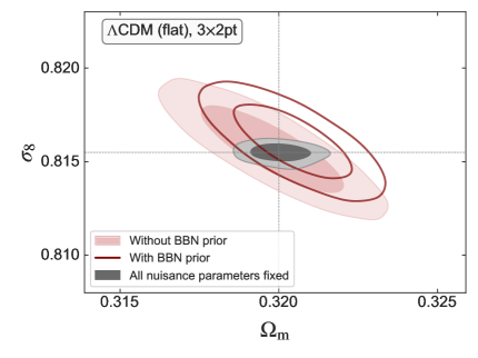
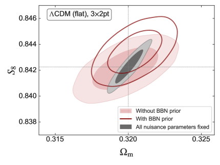
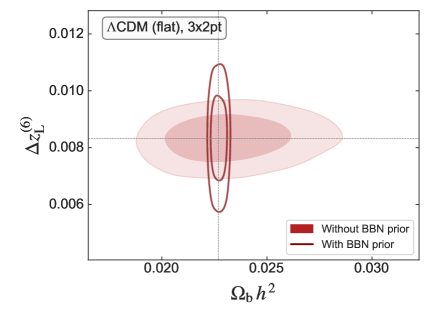
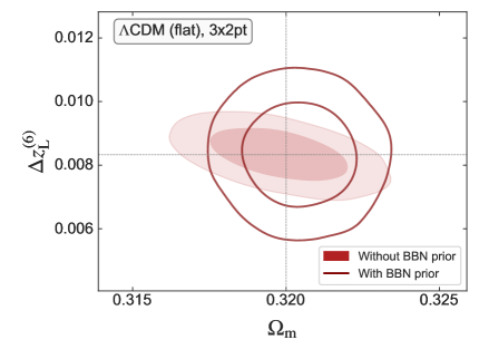
Figure 13: Two-dimensional posterior distributions for the cosmological parameters $\varOmega_{{\rm m}}$, $\sigma_{8}$ and $S_{8}$, $\varOmega_{{\rm b}}\,h^{2}$, and 6-redshift bin shift mean $\varDelta z^{(6)}_{\rm L}$ for the lensing probe, for the model $\Lambda\mathrm{CDM}$. We show cases with and without BBN prior (dark red unfilled and light red filled contours, respectively), keeping all nuisance parameters free, and with the BBN prior but keeping all nuisance parameters fixed (light grey filled contours). The case with BBN prior and free nuisance parameters shows significant projection effects in $\sigma_{8}$ and $S_{8}$.

6.3.2 Impact of the experimental nuisance parameters on the cosmological parameters

In this section, we evaluate the impact of fixing or sampling systematic nuisance parameters on the constraints on cosmological parameters within the context of a 3×2pt analysis, using high GCph scale cuts and a BBN prior. The focus is on the cosmological parameters for both the $\Lambda\mathrm{CDM}$ and $w_{0}w_{a}\mathrm{CDM}$ models, under the assumption of a flat geometric configuration. Specifically, we assess how the treatment of two key systematic nuisance parameters, the per-bin shear multiplicative bias $m_{i}$ and the mean redshift shifts $\varDelta z^{\rm L}_{i}$, influences the resulting cosmological constraints. These forecasts give insightful information about the current scientific requirements for Euclid, which were previously developed in Amara & Refregier (2008) and Massey et al. (2013) and provide a historical perspective of the mission design.

While some systematic nuisance parameters, such as intrinsic alignment, magnification, and galaxy biases are inherently dependent on the underlying cosmological or astrophysical models, $m_{\rm L}^{i}$ and $\varDelta z_{\rm L}^{i}$ are primarily determined by the experimental setup and the data processing pipeline. The Euclid data analysis pipeline and calibration efforts impose stringent requirements on these parameters, and this information is used to define informative priors during the cosmological inference exercise (see Table 2 for the imposed Gaussian priors on $m_{\rm L}^{i}$ and $\varDelta z_{\rm L}^{i}$). Our objective is to investigate whether these nuisance parameters can be ignored if Euclid’s requirements are met in DR3, and therefore, if they can be fixed during the inference analysis.

To address this question, we performed analyses with the same configuration as presented in Fig. 9, examining scenarios where $m_{\rm L}^{i}$ and $\varDelta z_{\rm L}^{i}$ are kept fixed for both the flat $\Lambda\mathrm{CDM}$ and $w_{0}w_{a}\mathrm{CDM}$ models (see Fig. 12). The resulting posterior distributions reveal that the results are model-dependent. In the $w_{0}w_{a}\mathrm{CDM}$ model, fixing these nuisance parameters leads to a significant impact on the marginalised uncertainties of key cosmological parameters such as $\sigma_{8}$ and $S_{8}$, and the dark energy equation of state parameters $w_{0}$ and $w_{a}$. This in turn results in a measurable change in the dark energy $\mathrm{FoM}$, with a higher value of 454, thus highlighting the importance of accounting for these systematics in the analysis.

In contrast, in the $\Lambda\mathrm{CDM}$ model, the effect of fixing these nuisance parameters during the inference analysis is minimal. The marginalised uncertainties for the cosmological parameters remain virtually unchanged, both at the 68 and 95 percent confidence levels. This result suggests that, for $\Lambda\mathrm{CDM}$, the influence of these particular nuisance parameters is less critical, allowing us to reduce the sampled parameter space significantly without inducing extra errors on the cosmological uncertainties. We have left for future work the analysis of the impact of experimental nuisance parameters in other cosmological models beyond the $\Lambda\mathrm{CDM}$ and $w_{0}w_{a}\mathrm{CDM}$ models.

6.3.3 Projection effects in $\Lambda\mathrm{CDM}$

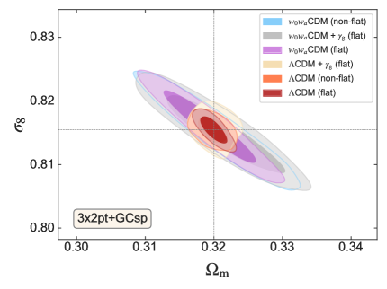
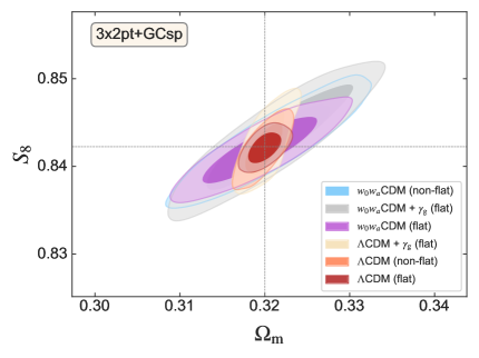
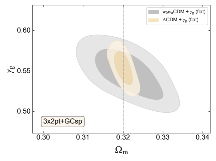
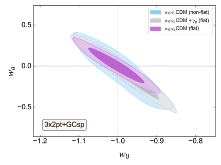
Figure 14: Two-dimensional posterior distributions for the cosmological parameters $\varOmega_{{\rm m}}$, $\sigma_{8}$ and $S_{8}$, $w_{0}$ and $w_{a}$, and $\varOmega_{{\rm m}}$ and $\gamma_{\mathrm{g}}$, using the full photometric probe combination (3×2pt) in combination with spectroscopic galaxy clustering full shape (GCsp). The values for the $\mathrm{FoM}$ of $w_{0}$ and $w_{a}$ can be found in Table 5.

When analysing the 3×2pt results in Fig. 9, we observe an evident shift in the one-dimensional posterior distributions of $\sigma_{8}$ and $S_{8}$ for the flat $\Lambda\mathrm{CDM}$ model. These shifts are due to the presence of a shift in the one-dimensional marginalised posterior distribution in the sampled parameters $\varOmega_{{\rm c}}\,h^{2}$ and $\ln(10^{10}A_{\rm s})$. We do not observe this behaviour in the results of the other cosmological models, most likely given that the uncertainties associated with the cosmological parameters in those cases are larger.

To verify if this is indeed a projection effect, we checked that the best-fit (that is, the minimum of the $\chi^{2}$) is recovered when the sampled parameters adopt the fiducial set of values. Moreover, we have checked if this effect is due to possible under-sampling of the parameter space, by increasing the number of live points and the number of trained neural networks of Nautilus, finding the same resulting posterior distributions. Furthermore, we have validated Nautilus for the Euclid study case against PolyChord, and we did not find significant differences in the sampled posterior distributions.

While the presence of projection effects has been reported in the usual sampled parameter space of LSS when conservative scale cuts and/or non-linear galaxy bias are used to model the 3×2pt probe and the nuisance parameters are left free, it is still novel to find projection effects within a $\Lambda\mathrm{CDM}$ framework. To assess the origin of these projection effects, we investigated two possible sources:

1. The large parameter space to sample: To check this hypothesis, we run several cases where we progressively fix all nuisance parameters and evaluate the marginalised posterior distributions for cosmological parameters.
   

2. Possible degeneracies between the experimental systematic nuisance parameters and the cosmological parameters in the presence of a BBN prior: To verify this hypothesis, we re-run the same 3×2pt $\Lambda\mathrm{CDM}$ case with all parameters free, but imposing a flat prior on $\varOmega_{{\rm b}}\,h^{2}$.

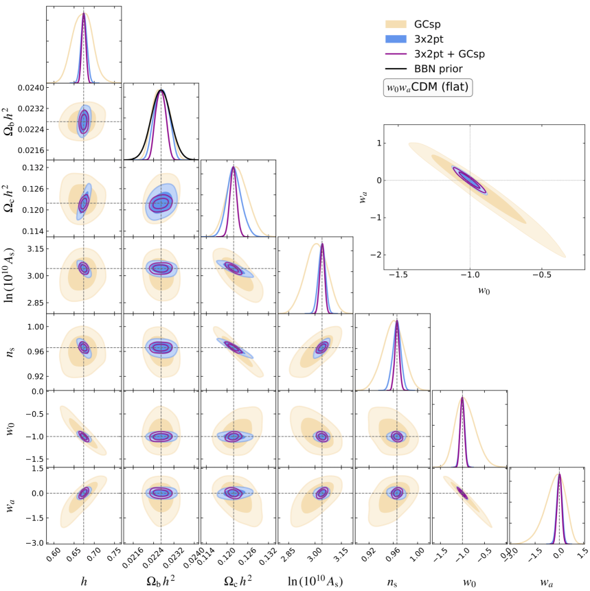
Figure 15: Forecast of the constraints for the $w_{0}w_{a}\mathrm{CDM}$ cosmological model (adopting a flat geometry) using only Euclid photometric and spectroscopic probes: spectroscopic galaxy clustering (GCsp), cosmic shear, galaxy-galaxy lensing and angular clustering, 3×2pt, and the combination of both of them as described in Sect. 6.4. For the photometric probes, we used $\ell_{\rm max}=5000$ for cosmic shear and $\ell_{\rm max}=3000$ for photometric angular clustering, and galaxy-galaxy lensing. The corresponding $\mathrm{FoM}$ obtained for each sample can be found at Table 5. We show, as a zoom-in, the 2-dimensional posterior distribution corresponding to the dark energy parameters $w_{0}$ and $w_{a}$.

The results of our hypothesis testing cases can be found in Fig. 13, where we show the corresponding two-dimensional posterior distributions for key cosmological parameters, as well as the degeneracy between some cosmological parameters and the per-bin redshift bin shift parameters. We conclude that the projection effects disappear when all nuisance parameters are kept fixed and the BBN prior is still imposed (see grey filled contours shown in the upper row of Fig. 13). Although not explicitly shown, the disappearance of projection effects is also found when all nuisance parameters are kept free except for the per-bin redshift bin shift mean parameters and when the BBN prior is still imposed within the analysis. On the other hand, when all nuisance parameters are kept open, but a flat prior is imposed on $\varOmega_{{\rm b}}\,h^{2}$, there are no projection effects (see red unfilled contours shown in the upper row of Fig. 13). We conclude that projection effects are therefore a consequence of the degeneracy between $\varOmega_{{\rm b}}\,h^{2}$ and all the 26 per-bin redshift bin shift mean parameters (for both cosmic shear and angular clustering), as observed in the lower left panel of Fig. 13. The BBN prior imposes tight one-dimensional constraints on $\varOmega_{{\rm b}}\,h^{2}$, allowing more freedom for $\varDelta z_{\rm L}^{i}$ to explore a broader parameter-value range within its Gaussian prior, despite the two-dimensional volume (light red area within the contour shown in the lower left panel of Fig. 13) being larger.

6.4 Full analysis: 3×2pt + GCsp

Combining photometric and spectroscopic probes unlocks the full potential of Euclid’s primary probes (see Fig. 14, and confidence intervals for all the cosmological and nuisance parameters for the $w_{0}w_{a}\mathrm{CDM}$ model in Appendix C). The photometric primary probes alone (3×2pt) tightly constrain $\varOmega_{{\rm m}}$ and $\sigma_{8}$, while spectroscopic galaxy clustering primarily constrains $\ln(10^{10}A_{\rm s})$, $H_{0}$ and $\varOmega_{K}$. For this analysis, we assume no correlation between spectroscopic and photometric probes (Euclid Collaboration: Paganin et al. 2024). The inclusion of GCsp data alongside the 3×2pt analysis significantly enhances constraints on several cosmological parameters and degeneracies are significantly reduced, particularly those related to the shape and amplitude and shape of the matter power spectrum.

The full one and two-dimensional posterior distributions for the cosmological parameters given the $w_{0}w_{a}\mathrm{CDM}$ flat model for spectroscopic galaxy clustering, 3×2pt and the full combination are shown in Fig. 15. Including spectroscopic galaxy clustering leads to a marked improvement in the confidence intervals for all cosmological parameters compared to the 3×2pt case. This includes tighter constraints on $\varOmega_{{\rm b}}$ (where the posterior becomes more informative than the BBN prior), $\varOmega_{{\rm m}}$, $H_{0}$ and $n_{\rm s}$. Notably, the uncertainty on $\varOmega_{{\rm c}}\,h^{2}$ improves by approximately 53%, highlighting the strong sensitivity of galaxy clustering to the matter density. Similarly, the scalar spectral index $n_{s}$ and the amplitude parameter $\ln(10^{10}A_{s})$ see relative improvements of 43% and 35%, respectively. The Hubble parameter $h$ and the baryon density $\varOmega_{{\rm c}}\,h^{2}$ also benefit from tighter constraints, with reductions in uncertainty of about 32% and 30%. These gains demonstrate the complementarity of GCsp with weak lensing and galaxy-galaxy lensing, especially in breaking degeneracies and enhancing sensitivity to early-universe parameters (see Table 6). The latter improvement on $n_{\rm s}$ arises from fixing several EFT parameters, as detailed in Sect. 6.2.

The full combination further constrains the sampled EFTofLSS spectroscopic nuisance parameters (see Appendix B, in particular Figs. 20 and 21) by breaking degeneracies with the cosmological parameters. In contrast, the spectroscopic galaxy clustering probe does not significantly improve constraints on the photometric nuisance parameters (see Figs. 17 and 20), as these are already dominated by their priors – specifically the photometric multiplicative bias and the per-bin redshift parameters given by Euclid science requirements. Best-fits of nuisance parameters for the $w_{0}w_{a}\mathrm{CDM}$ flat model are found in Table 8 and Table 9.

In our analysis, we find that certain cosmological parameters exhibit significant correlations with nuisance parameters, which can impact the robustness of cosmological inferences. Notably, $\varOmega_{{\rm c}}\,h^{2}$ shows strong negative correlations with several nuisance parameters associated with spectroscopic calibration, in particular the scale-independent shot noise terms, with values ranging around $-0.8$. Additionally, the spectral index $n_{s}$ itself is positively correlated with these parameters with values close to $-0.7$. These correlations, with absolute values often exceeding 0.7, indicate that marginalizing over nuisance parameters can substantially affect constraints on key cosmological quantities. Such findings underscore the importance of careful modelling and mitigation of systematics in cosmological analyses to avoid biased parameter estimation, as well as the importance of priors in these nuisance parameters.

We assess model selection for Euclid joint analyses of cosmological models using the Bayesian evidence $\ln{\cal Z}(\boldsymbol{d}\,|\,M)$, provided by Nautilus, where higher values indicate preferred models (see Table 7). Across all probes, the flat $\Lambda\mathrm{CDM}$ model consistently yields the highest evidence values, serving as the reference for model comparison. Extensions such as the inclusion of a time-varying dark energy equation of state ($w_{0}w_{a}\mathrm{CDM}$), non-flat geometries, or modifications to the growth index ($\gamma_{\mathrm{g}}$) lead to lower $\ln{\cal Z}(\boldsymbol{d}\,|\,M)$ values, reflecting a statistical penalty for the increased model complexity. Nevertheless, within the $w_{0}w_{a}\mathrm{CDM}$ family, the differences in $\ln{\cal Z}(\boldsymbol{d}\,|\,M)$ between the flat and non-flat models, or between those with and without $\gamma_{\mathrm{g}}$, remain relatively small – typically $\varDelta\ln{\cal Z}(\boldsymbol{d}\,|\,M)\lesssim 2$ – indicating that these extensions are not strongly disfavoured. This is consistent with Fig. 14, which shows that the inclusion of non-flatness or modified gravity does not significantly affect the constraints on $(w_{0},w_{a})$. This result is encouraging in the context of Euclid, as it demonstrates the capability of the survey to constrain multiple $\Lambda\mathrm{CDM}$ extensions simultaneously, rather than needing to isolate them due to strong degeneracies.

The $\mathrm{FoM}$ values obtained for $w_{0}$ and $w_{a}$ using the full combination of probes (see Table 5, last column) are consistent with the results presented in Euclid Collaboration: Blanchard et al. (2020). As in previous cases, our findings align with the predictions for the pessimistic scenario discussed in their study, despite adopting a higher maximum photometric multipole for 3×2pt in our analysis. This result can primarily be attributed to the extensive parameter space sampled in the current analysis, which spans 58 to 61 dimensions for the full statistical sampling exercise. Yet, we recover a $\mathrm{FoM}$ value for $w_{0}$ and $w_{a}$ above 400 for the flat $w_{0}w_{a}\mathrm{CDM}$ model, in agreement with the scientific performance specifications presented in the Euclid definition study report (Laureijs et al. 2011).

Altogether, the combination of all Euclid primary probes underscores that the mission will set the future benchmark for multi-probe large-scale structure cosmological analyses. Its constraining power on cosmological parameters is comparable to, or potentially surpasses, that of Planck. This conclusion holds robustly across all studied cosmological models, extending beyond the flat $w_{0}w_{a}\mathrm{CDM}$ scenarios.

7 Conclusions

In this study, we have presented a comprehensive analysis of the forecast results for Euclid’s primary probes across various cosmological models using CLOE. We have demonstrated that CLOE, when used with Cobaya and Nautilus, is able to produce robust forecasts that are easily reproducible by using Open Science tools such as ESA datalabs.

Our findings demonstrate the complementarity of weak lensing and spectroscopic galaxy clustering in constraining key cosmological parameters. We observed that, while WL provides strong constraints on $\varOmega_{{\rm m}}$ and $\sigma_{8}$, GCsp offers enhanced precision on primordial parameters such as $\ln(10^{10}A_{\rm s})$ and on the geometrical curvature of the Universe $\varOmega_{K}$. The 3×2pt combination of photometric probes further enhances the constraining power of Euclid, increasing the figure of merit for dark energy parameters by an order of magnitude compared to the single probes WL and GCsp. It also achieves at least an order of magnitude improvement in the uncertainty constraints for $\sigma_{8}$ and $\varOmega_{{\rm m}}$, and an order of magnitude improvement with respect to current galaxy surveys such as DES and KiDS.

We have demonstrated that the combination of angular clustering and galaxy-galaxy lensing provides most of the cosmological constraining power in the photometric 3×2pt analysis when compared with shear only. This conclusion is reached after studying the behaviour of GCph with low scale cuts. This highlights that further refinements in the theoretical modelling of galaxy clustering, including non-linear scales and systematic effects (visibility), are essential to reduce systematic uncertainties and improve the reliability of Euclid’s primary probes, thereby unlocking the full potential of the mission.

We have shown that model selection critically influences the interpretation of Euclid data, as different cosmological models impact posterior distributions and parameter degeneracies across all probes. Using Bayesian evidence $\ln{\cal Z}(\boldsymbol{d}\,|\,M)$ computed with Nautilus (see Table 7), the flat $\Lambda\mathrm{CDM}$ model consistently emerges as the preferred baseline. Although extensions such as $w_{0}w_{a}\mathrm{CDM}$, non-flat geometries, and modified growth index ($\gamma_{\mathrm{g}}$) face a statistical penalty for complexity, their evidence differences remain small ($\varDelta\ln{\cal Z}(\boldsymbol{d}\,|\,M)\lesssim 2$), indicating that they are not strongly disfavoured. This, along with minimal impact on $(w_{0},w_{a})$ constraints, underscores Euclid’s ability to simultaneously constrain multiple $\Lambda\mathrm{CDM}$ extensions without significant degeneracies. In any case, we note that our model selection results are derived under the assumption that the likelihood peaks exactly at $\Lambda\mathrm{CDM}$, the model for which the synthetic data vectors were generated. In practice, real survey and noise realisations may yield fluctuations that occasionally favour extended models such as $w_{0}w_{a}\mathrm{CDM}$, even if the ensemble average still prefers $\Lambda\mathrm{CDM}$. This effect, which is not captured in our current forecasts, is expected to moderate the decisive evidence differences reported here and will need to be carefully reassessed with real Euclid data.

Additionally, the sheer scale of the parameter space explored in this work has highlighted the importance of developing a robust strategy to secure and manage the computational resources needed to carry out a study of such a scale. In fact, the complexity of the models and the large number of parameters require significant computational power, which must be efficiently managed to ensure timely and accurate results. Our analysis also points to the need for exploring alternative sampling methods. The traditional approaches may struggle with the high dimensionality and non-Gaussian posteriors encountered in some of these analyses, which will, most likely, become more important when non-standard cosmological models are explored. Employing more sophisticated sampling techniques, such as Simulation-Based Inference (von Wietersheim-Kramsta et al. 2025; Jeffrey et al. 2025; Franco-Abelln et al. 2024) and Hamiltonian Monte Carlo (Bonici et al. 2023; Ruiz-Zapatero et al. 2024; Piras & Spurio Mancini 2023), could offer improved convergence and accuracy in parameter estimation, particularly for scenarios with a large number of free parameters.

Finally, our work suggests that achieving a realistic $\mathrm{FoM}$ greater than 400 requires the full combination of Euclid’s primary probes: 3×2pt and GCsp. Yet, while 2-point summary statistics of Euclid’s primary probes provide valuable insights on the dark energy parameters $w_{0}$ and $w_{a}$, incorporating information from Euclid higher-order statistical probes and external cosmological data sets could substantially enhance the overall statistical constraining power on a given cosmological model and reduce degeneracies among parameters. This will be crucial in pushing the boundaries of precision cosmology and extracting the maximum amount of information from future data releases.

Appendix A Computational resources

Table 7: Summary of the computational resources used during the forecast exercise using the sampler Nautilus, for all the observational probes and cosmological models.

Cosmology	Size	$\ln{\cal Z}(\boldsymbol{d}\,|\,M)$	Cluster	Wall-Time	CPUs
Weak Lensing (WL)
$\Lambda\mathrm{CDM}$ (flat)	$34$	$-29.52$	yggdrasil	2 days, 1 hour, 42 minutes	$24$
$\Lambda\mathrm{CDM}$ + $\gamma_{\mathrm{g}}$ (flat)	$35$	$-31.74$	yggdrasil	2 days, 11 hours, 14 minutes	$24$
$\Lambda\mathrm{CDM}$ (non-flat)	$35$	$-30.47$	yggdrasil	2 days, 10 hours, 39 minutes	$24$
$w_{0}w_{a}\mathrm{CDM}$ (flat)	$36$	$-33.70$	yggdrasil	7 days, 2 hours, 32 minutes	$24$
$w_{0}w_{a}\mathrm{CDM}$ + $\gamma_{\mathrm{g}}$ (flat)	$37$	$-34.81$	yggdrasil	3 days, 8 hours, 21 minutes	$24$
$w_{0}w_{a}\mathrm{CDM}$ (non-flat)	$37$	$-34.07$	yggdrasil	7 days, 16 hours, 15 minutes	$24$
Galaxy Clustering (GCsp)
$\Lambda\mathrm{CDM}$ (flat)	$21$	$-80.67$	yggdrasil	5 days, 18 hours, 24 minutes	$24$
$\Lambda\mathrm{CDM}$ + $\gamma_{\mathrm{g}}$ (flat)	$22$	$-81.88$	yggdrasil	6 days, 23 hours, 8 minutes	$24$
$\Lambda\mathrm{CDM}$ (non-flat)	$22$	$-82.20$	yggdrasil	7 days, 12 hours, 41 minutes	$24$
$w_{0}w_{a}\mathrm{CDM}$ (flat)	$23$	$-85.43$	yggdrasil	9 days, 14 hours, 37 minutes	$24$
$w_{0}w_{a}\mathrm{CDM}$ + $\gamma_{\mathrm{g}}$ (flat)	$23$	$-86.29$	yggdrasil	15 days, 8 hours, 31 minutes	$24$
$w_{0}w_{a}\mathrm{CDM}$ (non-flat)	$24$	$-86.07$	yggdrasil	12 days, 6 hours, 58 minutes	$24$
3×2pt
$\Lambda\mathrm{CDM}$ (flat)	$42$	$-124.69$	gouwezee	7 days, 7 hours, 45 minutes	$50$
$\Lambda\mathrm{CDM}$ (flat, no BBN prior)	$42$	$-127.32$	ketelmeer	4 days, 21 hours, 0 minutes	$50$
$\Lambda\mathrm{CDM}$ (flat, fixed nuisance)	$6$	$-20.19$	gouwezee	8 hours, 21 minutes	$50$
$\Lambda\mathrm{CDM}$ (flat, fixed systematic nuisance)	$16$	$-82.83$	ketelmeer	3 days, 2 hours, 35 minutes	$24$
$\Lambda\mathrm{CDM}$ + $\gamma_{\mathrm{g}}$ (flat)	$43$	$-128.06$	eemmeer	9 days, 4 hours, 17 minutes	$50$
$\Lambda\mathrm{CDM}$ (non-flat)	$43$	$-127.09$	xmaris	10 days, 12 hours, 52 minutes	$50$
$w_{0}w_{a}\mathrm{CDM}$ (flat)	$44$	$-131.59$	amsteldiep	11 days, 16 hours, 29 minutes	$50$
$w_{0}w_{a}\mathrm{CDM}$ (flat, low GCph scale cuts)	$44$	$-107.44$	baobab	5 days, 6 hours, 16 minutes	$50$
$w_{0}w_{a}\mathrm{CDM}$ (flat, fixed nuisance)	$8$	$-35.77$	gouwezee	1 day, 16 hours, 50 minutes	$50$
$w_{0}w_{a}\mathrm{CDM}$ (flat, fixed systematic nuisance)	$18$	$-90.32$	ketelmeer	2 days, 15 hours, 43 minutes	$50$
$w_{0}w_{a}\mathrm{CDM}$ + $\gamma_{\mathrm{g}}$ (flat)	$45$	$-134.82$	markermeer	15 days, 5 hours, 19 minutes	$50$
$w_{0}w_{a}\mathrm{CDM}$ (non-flat)	$45$	$-133.69$	eemmeer	21 days, 1 hours, 6 minutes	$50$
2×2pt
$w_{0}w_{a}\mathrm{CDM}$ (flat, low GCph scale cuts)	$44$	$-104.48$	baobab	5 days, 2 hours, 27 minutes	$50$
3×2pt + GCsp
$\Lambda\mathrm{CDM}$ (flat)	$58$	$-192.02$	meluxina	19 days, 2 hours, 32 minutes	$100$
$\Lambda\mathrm{CDM}$ + $\gamma_{\mathrm{g}}$ (flat)	$59$	$-196.26$	meluxina	9 days, 3 hours, 26 minutes	$100$
$\Lambda\mathrm{CDM}$ (non-flat)	$59$	$-195.46$	baobab	11 days, 19 hours, 58 minutes	$100$
$w_{0}w_{a}\mathrm{CDM}$ (flat)	$60$	$-200.38$	ketelmeer	9 days, 11 hours, 39 minutes	$100$
$w_{0}w_{a}\mathrm{CDM}$ + $\gamma_{\mathrm{g}}$ (flat)	$61$	$-202.58$	baobab	24 days, 14 hours, 53 minutes	$100$
$w_{0}w_{a}\mathrm{CDM}$ (non-flat)	$61$	$-201.08$	baobab	28 days, 13 hours, 9 minutes	$100$

Note: We specify the size of the parameter space, the value of the log-evidence $\ln{\cal Z}(\boldsymbol{d}\,|\,M)$ when the run converges, the name of the cluster, the total computational wall running time and the number of CPUs used to parallelise the likelihood calls (pool multithreading). On top of these resources, if available (i.e: machines used to run 3×2pt and 3×2pt + GCsp), another 16 or 24 CPUs in total were employed to speed up the CAMB transfer function calculation when necessary. If not specified, the scale-cuts used for GCph and XC were $\ell=3000$. If specified as low GCph scale cuts, they correspond to $\ell=750$ for GCph and XC as listed in Table 1.

The computational effort required for this research work is considerable, reflecting the complexity and scale of cosmological modeling and data analysis involved. The main bottleneck in the calculation arises from the theory calculations (approximately 2 seconds for both 3×2pt and spectroscopic galaxy clustering full-shape analyses, including the Boltzmann solver call to obtain the matter power spectrum) and from sampling across the large parameter space. In total, this paper utilises over half of a million CPU hours for a variety of cosmological models and cosmological probes, such as weak lensing (WL), spectroscopic galaxy clustering (GCsp), and the combination of different data sets (3×2pt analysis, and 3×2pt + GCsp). Details on the computational resources used for each exercise using the Nautilus sampler can be found at Table 7. The clusters gouwezee, ketelmeer, eemmeer, amsteldiep, and markermeer are located at Leiden Observatory (The Netherlands). The clusters yggdrasil and baobab are hosted by the University of Geneva (Switzerland). The cluster xmaris (now part of the cluster Alice) is located at Leiden University (The Netherlands). The cluster meluxina was accessed through a EuroHPC Joint Undertaking grant at LuxProvide (Luxembourg).

For weak lensing alone, the computational cost reaches nearly 22,000 CPU hours. Galaxy clustering analyses needed about 50,000 CPU hours. The 3×2pt analysis, combining weak lensing, galaxy clustering, and galaxy-galaxy lensing for all the different tests carried out in this research represents the second-to-first most computationally demanding part of the research, summing up over 176,000 CPU hours. Finally, the most computationally expensive case is the full Euclid analysis combining 3×2pt with galaxy clustering, reaching up to 247,000 CPU hours. Overall, the results indicate that the more complex the parameter space – whether due to higher dimensionality or stronger degeneracies – the longer the computational time required for sampling, although specific scalability tests might be indicated for future studies. If this forecast exercise had been done with PolyChord, the total computational cost would have been roughly 2 million CPU hours. We found that the MH MCMC algorithm in Cobaya is not suitable for sampling such a large parameter space.

Appendix B Nuisance-parameter posterior distributions

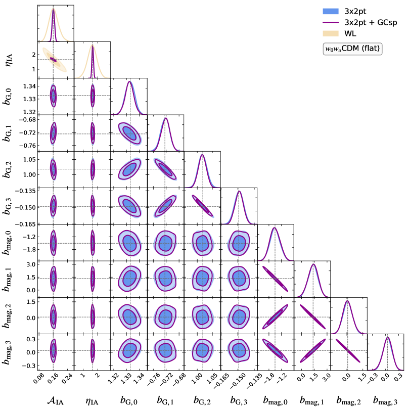
Figure 16: Forecast of the constraints for the photometric nuisance parameters of the $w_{0}w_{a}\mathrm{CDM}$ cosmological model (adopting a flat geometry) using Euclid photometric and spectroscopic probes: cosmic shear (WL), cosmic shear, galaxy-galaxy lensing and angular clustering (3×2pt), and the combination of both of them as described in Sect. 6.4 (3×2pt + GCsp). For the photometric probes, we used $\ell_{\rm max}=5000$ for cosmic shear and $\ell_{\rm max}=3000$ for photometric angular clustering, and galaxy-galaxy lensing. We show, as zoom-in, the 2-dimensional posterior distribution corresponding to the intrinsic alignment parameters $\mathcal{A}_{\mathrm{IA}}$ and $\eta_{\mathrm{IA}}$.

In this section, we present the posterior distributions of all the sampled and some derived nuisance parameters for WL, 3×2pt, and GCsp within the $w_{0}w_{a}\mathrm{CDM}$ cosmological model, including single probes, the combined 3×2pt analysis, and the joint 3×2pt + GCsp analysis. By providing the full set of posteriors, we aim to ensure transparency and enable reproducibility of our results in future work. Additionally, this comprehensive presentation highlights the complexity and vast dimensionality of the parameter space sampled in our analyses. Definitions of each parameter are detailed in Table 2. If a Gaussian prior was used, this is showcased as example.

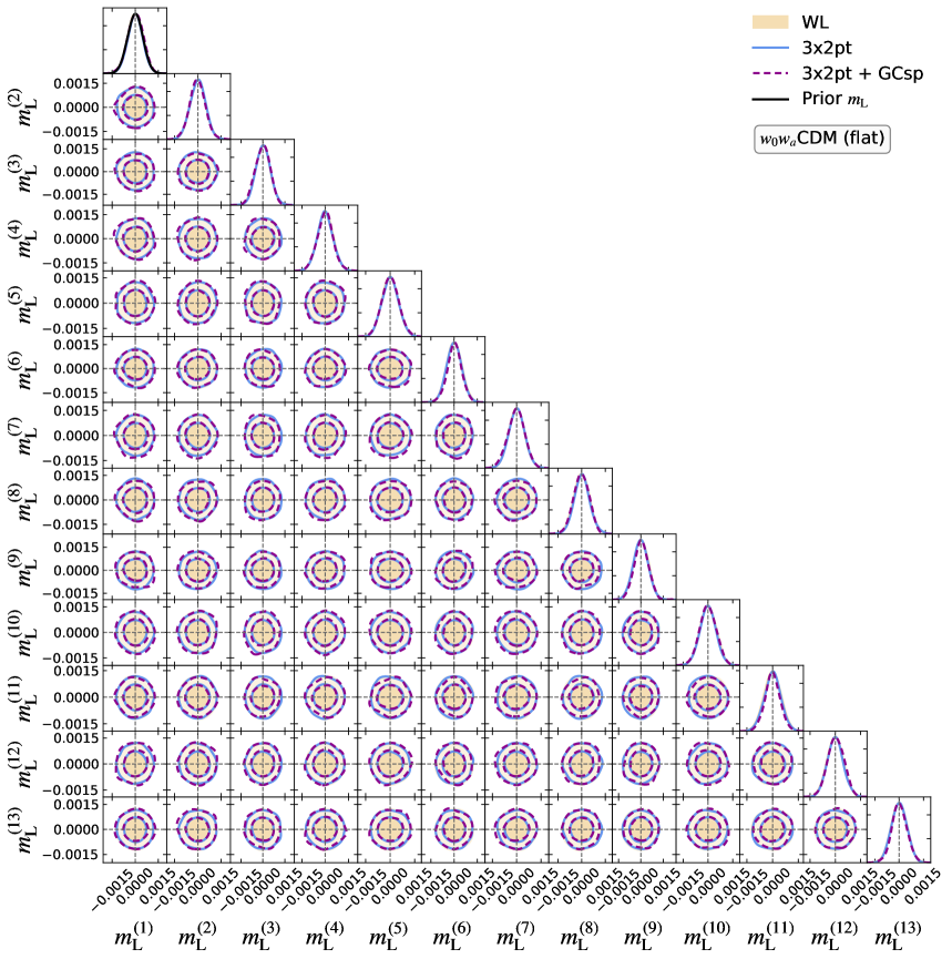
Figure 17: Forecast of the constraints for the photometric nuisance parameters of the $w_{0}w_{a}\mathrm{CDM}$ cosmological model (adopting a flat geometry) using Euclid photometric and spectroscopic probes: cosmic shear (WL), cosmic shear, galaxy-galaxy lensing and angular clustering (3×2pt), and the combination of both of them as described in Sect. 6.4 (3×2pt + GCsp). For the photometric probes, we used $\ell_{\rm max}=5000$ for cosmic shear and $\ell_{\rm max}=3000$ for photometric angular clustering, and galaxy-galaxy lensing.

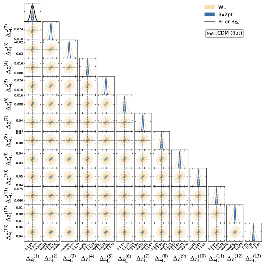
Figure 18: Forecast of the constraints for the photometric nuisance parameters of the $w_{0}w_{a}\mathrm{CDM}$ cosmological model (adopting a flat geometry) using Euclid photometric probes: cosmic shear (WL), and cosmic shear, galaxy-galaxy lensing and angular clustering (3×2pt). For the photometric probes, we used $\ell_{\rm max}=5000$ for cosmic shear and $\ell_{\rm max}=3000$ for photometric angular clustering, and galaxy-galaxy lensing. The degeneracy between adjacent bins is evident.

Although not explicitly shown for all parameters, the analysis of $w_{0}w_{a}\mathrm{CDM}$, adopting a flat geometry and joint full Euclid analysis, reveals that several nuisance parameters exhibit exceptionally strong mutual correlations, both positive and negative, which can have significant implications for parameter inference. Notably, in Fig. 16, we can see that the polynomial photometric galaxy bias parameters and the polynomial magnification bias parameters show strong positive and negative correlations, although not among them. For example, all polynomial magnification bias parameters are heavily (anti)-correlated with absolute values up to $0.9$. The photometric galaxy bias parameters also display strong correlations, such as $b_{\mathrm{G,1}}$ vs. $b_{\mathrm{G,2}}$ ($-0.905$) and $b_{\mathrm{G,1}}$ vs. $b_{\mathrm{G,3}}$ ($0.860$). Overall, the nuisance parameters shown in Fig. 16 are well constrained and remain within the specified prior ranges. The inclusion of the GCsp data does not lead to significantly tighter constraints on the photometric galaxy bias, magnification bias, or intrinsic alignment parameters. This is expected, as the 3×2pt combination already provides substantially stronger constraining power than GCsp alone, and the addition of GCsp does not break any further parameter degeneracies. This last behaviour is also observed on multiplicative biases shown in Fig. 17.

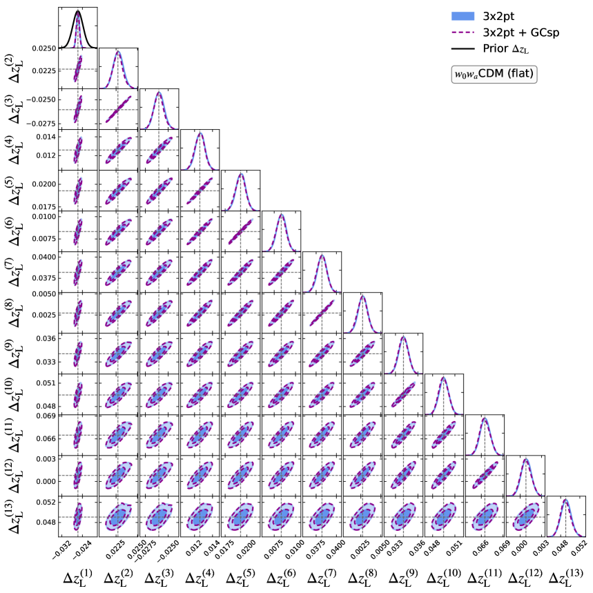
Figure 19: Forecast of the constraints for the photometric nuisance parameters of the $w_{0}w_{a}\mathrm{CDM}$ cosmological model (adopting a flat geometry) using Euclid photometric and spectroscopic probes: cosmic shear, galaxy-galaxy lensing and angular clustering (3×2pt), and the combination of both of them as described in Sect. 6.4 (3×2pt + GCsp). For the photometric probes, we used $\ell_{\rm max}=5000$ for cosmic shear and $\ell_{\rm max}=3000$ for photometric angular clustering, and galaxy-galaxy lensing. The degeneracy between adjacent bins is evident.

Multiplicative biases are also well constrained but remain prior-dominated, regardless of the data combination used. This is expected, as the priors imposed on these parameters (see, for example, the multiplicative bias prior associated with the first redshift bin in Fig. 17) are based on the assumption that the Euclid science requirements are met – requirements that are already highly constraining. Although not explicitly shown, the multiplicative biases exhibit mild degeneracies with $\sigma_{8}$ and $\ln(10^{10}A_{\rm s})$, as all three affect the amplitude of the power spectra.

The per-bin redshift shift nuisance parameters for the lensing sample, shown in Fig. 18, are well constrained but remain prior-dominated when using WL data alone. This is expected, given the stringent Euclid science requirements. However, when the full photometric 3×2pt combination is considered, these parameters are no longer dominated by the prior. For instance, the posterior for the first redshift bin shift parameter, shown in Fig. 19, illustrates this transition (may the reader note that other plotting scale is applied to the rest of the two-dimensional distributions to highlight the results when GCsp is also incorporated). This improvement is anticipated, as these redshift shift parameters are strongly correlated with $\varOmega_{{\rm b}}$ and $\varOmega_{{\rm c}}$, which are poorly constrained in the WL-only case but better determined in the 3×2pt analysis. This enhanced constraining power helps to break degeneracies and allows the redshift nuisance parameters to be more tightly constrained by the data. Similarly to the case of photometric galaxy and magnification biases, GCsp data do not further constrain per-bin redshift shift nuisance parameters (see purple contours in Fig. 19).

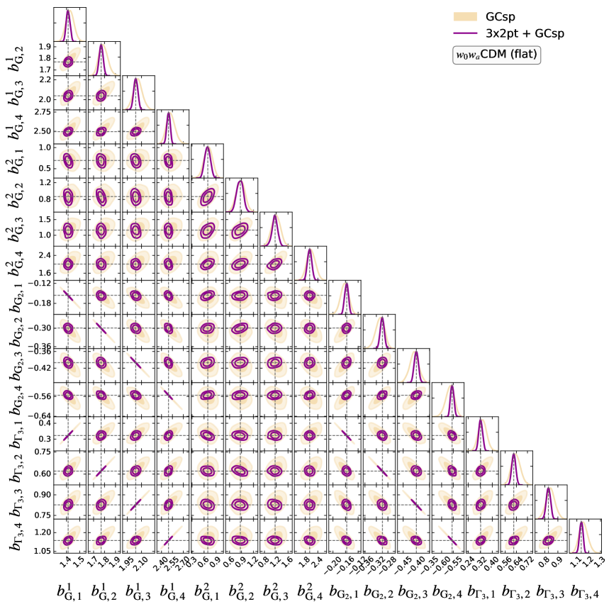
Figure 20: Forecast of the constraints for the spectroscopic nuisance parameters of the $w_{0}w_{a}\mathrm{CDM}$ cosmological model (adopting a flat geometry) using Euclid photometric and spectroscopic probes: spectroscopic galaxy clustering only (GCsp), and the combination with3×2ptas described in Sect. 6.4 (3×2pt + GCsp).

On the other hand, the spectroscopic galaxy bias nuisance parameters, while well constrained within their priors, exhibit non-Gaussian posteriors when sampled in isolation using the GCsp probe only. This behaviour is significantly mitigated when the full photometric probe is included in the analysis, leading to a notable reduction in the uncertainties of their best-fit values (see Fig. 20 and Table 9). This is due to strong correlations between these parameters and $\ln(10^{10}A_{\rm s})$, $\varOmega_{{\rm b}}$ and $\varOmega_{{\rm c}}$. The figure also includes derived parameters – those showing strong correlations – computed according to the prescriptions outlined in Table 2.

Further improvements in the constraints of spectroscopic nuisance parameters are observed in the calibration and purity parameters when 3×2pt data are included (see Fig. 21). In particular, the spectroscopic calibration parameters $\alpha_{\rm P}^{2}$, $\alpha_{\rm P}^{3}$, and $\alpha_{\rm P}^{4}$ exhibit strong mutual correlations, with correlation coefficients of $0.763$, $0.790$, and $0.909$, respectively. The calibration parameters are heavily correlated with $n_{\rm s}$. The purity parameters, which are all sampled from Gaussian priors (see an example of the Gaussian prior distribution used in the purity parameter associated to the first redshift bin in Fig. 21) are mildly correlated with the cosmological parameters.

In conclusion, the observed correlations among nuisance parameters underscore the importance of careful modelling and regularisation in cosmological analyses, as they can propagate into degeneracies and uncertainties in the cosmological parameter estimates (see illustrative examples in Sect. 6.3).

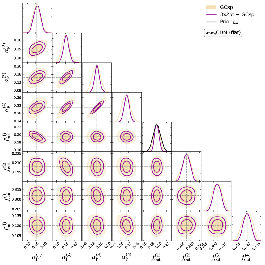
Figure 21: Forecast of the constraints for the spectroscopic nuisance parameters of the $w_{0}w_{a}\mathrm{CDM}$ cosmological model (adopting a flat geometry) using Euclid photometric and spectroscopic probes: spectroscopic galaxy clustering only (GCsp), and the combination with 3×2pt as described in Sect. 6.4 (3×2pt + GCsp).

Appendix C Confidence intervals of nuisance parameters for the $w_{0}w_{a}\mathrm{CDM}$ model

In this section, we list in Tables 6, 9 and 8 the 68% confidence limits of the sampled parameters corresponding to both the cosmological and the nuisance parameters for WL, 3×2pt and GCsp for the $w_{0}w_{a}\mathrm{CDM}$ cosmological model for single probes, combination 3×2pt and joint analysis 3×2pt + GCsp. The definition of each parameter can be found in Table 2.

Table 8: Same as Table 6, but for the photometric nuisance parameters.

	WL	3×2pt	3×2pt + GCsp
$\operatorname{log_{10}}({T_{\rm AGN}}/$K)	$7.743\pm 0.067$	$7.750\pm 0.015$	$7.749^{+0.014}_{-0.012}$
$\mathcal{A}_{\rm IA}$	$0.163^{+0.024}_{-0.029}$	$0.1605\pm 0.0063$	$0.1609\pm 0.0064$
$\eta_{\rm IA}$	$1.62\pm 0.33$	$1.658\pm 0.051$	$1.654\pm 0.050$
$\varDelta z_{\rm L}^{(1)}$	$-0.0257\pm 0.0022$	$-0.02571\pm 0.00058$	$-0.02575\pm 0.00058$
$\varDelta z_{\rm L}^{(2)}$	$0.0227\pm 0.0020$	$0.02276\pm 0.00058$	$0.02271\pm 0.00057$
$\varDelta z_{\rm L}^{(3)}$	$-0.0260\pm 0.0020$	$-0.02599\pm 0.00055$	$-0.02603\pm 0.00054$
$\varDelta z_{\rm L}^{(4)}$	$0.0127\pm 0.0019$	$0.01262\pm 0.00054$	$0.01259\pm 0.00054$
$\varDelta z_{\rm L}^{(5)}$	$0.0194\pm 0.0020$	$0.01931\pm 0.00057$	$0.01928\pm 0.00056$
$\varDelta z^{(6)}_{\rm L}$	$0.0084\pm 0.0020$	$0.00835\pm 0.00057$	$0.00831\pm 0.00056$
$\varDelta z_{\rm L}^{(7)}$	$0.0383\pm 0.0022$	$0.03823\pm 0.00059$	$0.03820\pm 0.00059$
$\varDelta z_{\rm L}^{(8)}$	$0.0028\pm 0.0022$	$0.00276\pm 0.00060$	$0.00272\pm 0.00060$
$\varDelta z_{\rm L}^{(9)}$	$0.0341\pm 0.0024$	$0.03409\pm 0.00064$	$0.03405\pm 0.00063$
$\varDelta z_{\rm L}^{(10)}$	$0.0494\pm 0.0026$	$0.04952\pm 0.00065$	$0.04948\pm 0.00063$
$\varDelta z_{\rm L}^{(11)}$	$0.0661\pm 0.0030$	$0.06653\pm 0.00069$	$0.06649\pm 0.00070$
$\varDelta z_{\rm L}^{(12)}$	$0.0007\pm 0.0035$	$0.00086\pm 0.00070$	$0.00081\pm 0.00071$
$\varDelta z_{\rm L}^{(13)}$	$0.0487\pm 0.0051$	$0.0491\pm 0.0011$	$0.04904^{+0.00097}_{-0.0011}$
$m_{\rm L}^{(1)}$	$0.00000\pm 0.00050$	$0.00001\pm 0.00049$	$0.00002\pm 0.00051$
$m_{\rm L}^{(2)}$	$0.00000\pm 0.00050$	$0.00000\pm 0.00050$	$-0.00003\pm 0.00050$
$m_{\rm L}^{(3)}$	$0.00000\pm 0.00050$	$0.00001\pm 0.00050$	$-0.00002\pm 0.00050$
$m_{\rm L}^{(4)}$	$0.00000\pm 0.00050$	$-0.00001\pm 0.00050$	$0.00000\pm 0.00051$
$m_{\rm L}^{(5)}$	$0.00000\pm 0.00050$	$0.00001\pm 0.00050$	$0.00001\pm 0.00051$
$m_{\rm L}^{(6)}$	$0.00001\pm 0.00050$	$0.00000\pm 0.00049$	$0.00002\pm 0.00046$
$m_{\rm L}^{(7)}$	$0.00000\pm 0.00049$	$0.00000\pm 0.00049$	$-0.00003\pm 0.00052$
$m_{\rm L}^{(8)}$	$0.00000\pm 0.00050$	$0.00002\pm 0.00049$	$-0.00002\pm 0.00049$
$m_{\rm L}^{(9)}$	$0.00001\pm 0.00050$	$-0.00001\pm 0.00050$	$0.00004\pm 0.00048$
$m_{\rm L}^{(10)}$	$0.00001\pm 0.00050$	$0.00000\pm 0.00049$	$0.00000\pm 0.00050$
$m_{\rm L}^{(11)}$	$-0.00001\pm 0.00050$	$0.00000\pm 0.00048$	$-0.00001\pm 0.00044$
$m_{\rm L}^{(12)}$	$-0.00001\pm 0.00048$	$0.00001\pm 0.00047$	$0.00004\pm 0.00049$
$m_{\rm L}^{(13)}$	$-0.00001\pm 0.00050$	$0.00000\pm 0.00048$	$0.00002\pm 0.00047$
$b_{{\rm G},\,0}$		$1.3327\pm 0.0036$	$1.3324\pm 0.0034$
$b_{{\rm G},\,1}$		$-0.723\pm 0.014$	$-0.722\pm 0.013$
$b_{{\rm G},\,2}$		$1.017\pm 0.015$	$1.017\pm 0.013$
$b_{{\rm G},\,3}$		$-0.1489\pm 0.0041$	$-0.1487\pm 0.0037$
$b_{{\rm mag},\,0}$		$-1.51\pm 0.24$	$-1.51\pm 0.24$
$b_{{\rm mag},\,1}$		$1.35\pm 0.58$	$1.35\pm 0.58$
$b_{{\rm mag},\,2}$		$0.08\pm 0.44$	$0.08\pm 0.44$
$b_{{\rm mag},\,3}$		$0.04\pm 0.10$	$0.04\pm 0.10$

Table 9: Same as Table 6, but for the spectroscopic nuisance parameters.

	GCsp	3×2pt + GCsp
$\alpha_{\rm P}^{(1)}$	$0.054\pm 0.024$	$0.058\pm 0.020$
$\alpha_{\rm P}^{(2)}$	$0.151\pm 0.021$	$0.154\pm 0.015$
$\alpha_{\rm P}^{(3)}$	$0.143\pm 0.020$	$0.146\pm 0.013$
$\alpha_{\rm P}^{(4)}$	$0.308\pm 0.021$	$0.311\pm 0.013$
$b^{1}_{\rm G,\,1}$	$1.426\pm 0.031$	$1.412\pm 0.014$
$b^{1}_{\rm G,\,2}$	$1.789^{+0.037}_{-0.043}$	$1.769\pm 0.017$
$b^{1}_{\rm G,\,3}$	$2.062\pm 0.048$	$2.039\pm 0.021$
$b^{1}_{\rm G,\,4}$	$2.527^{+0.053}_{-0.064}$	$2.496\pm 0.022$
$b^{2}_{\rm G,\,1}$	$0.70\pm 0.11$	$0.686\pm 0.068$
$b^{2}_{\rm G,\,2}$	$0.88\pm 0.11$	$0.860\pm 0.081$
$b^{2}_{\rm G,\,3}$	$1.19\pm 0.15$	$1.151\pm 0.095$
$b^{2}_{\rm G,\,4}$	$2.08\pm 0.20$	$2.005\pm 0.099$
$f_{\rm out}^{(1)}$	$0.1948\pm 0.0075$	$0.1949\pm 0.0057$
$f_{\rm out}^{(2)}$	$0.2039^{+0.0077}_{-0.0069}$	$0.2038\pm 0.0058$
$f_{\rm out}^{(3)}$	$0.3056\pm 0.0071$	$0.3058\pm 0.0056$
$f_{\rm out}^{(4)}$	$0.1209\pm 0.0073$	$0.1208\pm 0.0055$
$b_{{\rm G_{2}},\,1}$	$-0.163\pm 0.013$	$-0.1567\pm 0.0058$
$b_{{\rm G_{2}},\,2}$	$-0.307^{+0.016}_{-0.014}$	$-0.2997\pm 0.0067$
$b_{{\rm G_{2}},\,3}$	$-0.408\pm 0.017$	$-0.4002\pm 0.0077$
$b_{{\rm G_{2}},\,4}$	$-0.564^{+0.020}_{-0.017}$	$-0.5547\pm 0.0071$
$b_{{\varGamma_{3}},\,1}$	$0.335\pm 0.027$	$0.323\pm 0.012$
$b_{{\varGamma_{3}},\,2}$	$0.637^{+0.029}_{-0.034}$	$0.621\pm 0.014$
$b_{{\varGamma_{3}},\,3}$	$0.844\pm 0.035$	$0.827\pm 0.016$
$b_{{\varGamma_{3}},\,4}$	$1.156^{+0.034}_{-0.039}$	$1.137\pm 0.014$

The Gaussian priors set for the baryonic feedback parameter, multiplicative bias, photometric per-bin redshift bins and spectroscopic purity nuisance parameters establish baseline $\sigma$-uncertainties of $0.18$, $0.0005$, $0.01$, and approximately $0.002$, respectively. Comparing these prior widths to the best-fit posterior constraints presented in Table 8 and Table 9 reveals a significant tightening of the parameter estimates. To quantify the improvement in constraint precision, we define the tightening factor as the ratio between the prior standard deviation and the posterior standard deviation, i.e., $T\equiv\sigma_{\mathrm{prior}}/\sigma_{\mathrm{posterior}}$. Applying this definition, we find tightening factors of approximately $2.3$ for the multiplicative bias, $1.6$ for spectroscopic purity parameters, $3.3$ for the per-bin redshift shifts and $4.7$ for the baryonic feedback amplitude. These results demonstrate that the data significantly sharpen our knowledge of these nuisance parameters, reducing their uncertainties well below the levels assumed a priori and thus improving the robustness of the cosmological inference both at theoretical and observational level.