Score-Based Density Estimation
from Pairwise Comparisons

Abstract

We study density estimation from pairwise comparisons, motivated by expert knowledge elicitation and learning from human feedback. We relate the unobserved target density to a tempered winner density (marginal density of preferred choices), learning the winner’s score via score-matching. This allows estimating the target by ‘de-tempering’ the estimated winner density’s score. We prove that the score vectors of the belief and the winner density are collinear, linked by a position-dependent tempering field. We give analytical formulas for this field and propose an estimator for it under the Bradley-Terry model. Using a diffusion model trained on tempered samples generated via score-scaled annealed Langevin dynamics, we can learn complex multivariate belief densities of simulated experts, from only hundreds to thousands of pairwise comparisons.

1 Introduction

Several complementary techniques, from flows (Rezende & Mohamed, 2015; Lipman et al., 2023) to diffusion models (Ho et al., 2020), can today efficiently learn complex densities $p(\mathbf{x})$ from examples $\mathbf{x}\sim p(\mathbf{x})$. With sufficiently large data, we can learn accurate densities even over high-dimensional spaces, such as natural images (Rombach et al., 2022). While challenges persist in the most complex cases, these models have achieved a high level of performance, proving sufficient for many tasks.

We consider the fundamentally more challenging problem of learning the density not from direct observations but solely from comparisons of two candidates. Given $\mathbf{x}$ and $\mathbf{x}^{\prime}$ that are not sampled from the target $p(\mathbf{x})$ but rather from a distinct sampling distribution $\lambda(\mathbf{x})$ satisfying suitable regularity conditions, the task is to learn $p(\mathbf{x})$ from triplets $(\mathbf{x},\mathbf{x}^{\prime},\mathbf{x}\succ\mathbf{x}^{\prime})$. The last entry indicates which alternative has higher density (the winner point). Being able to do this enables, for instance, cognitively easy elicitation of human prior beliefs for statistical modeling (O’Hagan, 2019; Mikkola et al., 2023), or learning an implicit preference distribution for a generative model (Dumoulin et al., 2024). Our main interest is in representing human beliefs over relatively low-dimensional spaces – a person cannot realistically maintain a joint belief over more than a handful of variables – but we are also heavily constrained by the number of triplets, working with e.g. hundreds in contrast to millions in modern density learning works (Wang et al., 2023). In summary, we face two difficulties: (a) We do not have samples from the target density, and (b) we have extremely limited data in general.

Recently, Mikkola et al. (2024) proposed the first solution for this problem, learning normalizing flows from pairwise comparisons and rankings. We propose an improved solution that also uses random utility models (RUMs; Train, 2009) for modeling the preferential data and is inspired by their idea of relating the target density $p(\mathbf{x})$ to a tempered version of the distribution of winner points, $p_{w}^{\tau}(\mathbf{x})$, for some tempering parameter $\tau\geq 1$. Since we have samples from $p_{w}(\mathbf{x})$, this relationship leads to practical algorithms once $\tau$ is estimated. In contrast to their empirically motivated heuristic link, we characterize this connection in detail and provide an exact relationship between the scores of $p(\mathbf{x})$ and $p_{w}(\mathbf{x})$. Since the relationship holds for the scores, it is natural to also switch to solving the problem with score-based models (Song & Ermon, 2019; Song et al., 2021), instead of flows. This brings additional benefits, for instance in modeling multimodal targets, and we empirically demonstrate a substantial improvement in accuracy compared to Mikkola et al. (2024). While they could learn densities from a modest number of rankings, they needed additional regularization to avoid escaping probability mass (Nicoli et al., 2023). Moreover, their best accuracy required more informative multiple-item rankings. In contrast, we focus solely on pairwise comparisons, which are easier to answer and more reliable (Kendall & Babington Smith, 1940; Shah & Oppenheimer, 2008), and widely used in AI alignment (Ouyang et al., 2022; Wallace et al., 2024).

$\times$

(a) (a) Problem setup. An expert holds a subjective belief over a parameter space, such as the likely hyperparameters of a learning algorithm (e.g. learning rate and weight decay), and can answer questions like "Do you expect configuration A or B to work better?". We learn their belief as a density, to be used e.g. as a prior distribution for finding optimal hyperparameters. (b)-(d) Density estimation from $200$ uniformly sampled pairwise comparisons, with the target density shown as a heatmap. (b) Samples and the score field at an intermediate noise level $\sigma$, for a diffusion model trained on the (winner, loser) pairs to model the marginal winner density (MWD). (c) Estimated tempering field. (d) Samples from the score-scaled annealed Langevin dynamics with the MWD score and a tempering field estimate. Samples align well with the target density, demonstrating the fundamental relationship between the scores of the estimable MWD and the latent target (belief density).

Denote by $p_{\mathbf{x}\succ\mathbf{x}^{\prime}}(\mathbf{x},\mathbf{x}^{\prime})$ the joint density of the available data, encoding the preferred candidate in the order of the arguments. The marginal winner density (MWD), denoted by $p_{w}(\mathbf{x})$, is obtained as its marginal as $p_{w}(\mathbf{x})=\int p_{\mathbf{x}\succ\mathbf{x}^{\prime}}(\mathbf{x},\mathbf{x}^{\prime})d\mathbf{x}^{\prime}\propto\int\mathbb{P}(\mathbf{x}\succ\mathbf{x}^{\prime})\lambda(\mathbf{x})\lambda(\mathbf{x}^{\prime})d\mathbf{x}^{\prime}$ where $\lambda(\mathbf{x})$ is the sampling density of the (independent) candidates. Our main theoretical contribution is a novel, exact relationship between the target $p(\mathbf{x})$ and the MWD $p_{w}(\mathbf{x})$ in terms of their scores: up to a reparametrization of the space, we have $\nabla\log p(\mathbf{x})=\tau(\mathbf{x})\nabla\log p_{w}(\mathbf{x})$. Critically, $\tau(\mathbf{x})$ is not constant but a position-dependent tempering field. This implies we can perfectly recover $p(\mathbf{x})$ from the estimable $p_{w}(\mathbf{x})$ with score-based methods if the tempering field is known. We prove this foundational relationship for the popular Bradley–Terry model (Bradley & Terry, 1952; Touvron et al., 2023) and an exponential noise RUM, providing explicit formulas for the tempering fields.

Our second contribution is a practical algorithm derived from our theoretical insights. First, we propose to model the preference relationships by estimating the score of the joint density $p_{\mathbf{x}\succ\mathbf{x}^{\prime}}(\mathbf{x},\mathbf{x}^{\prime})$, then train a continuous-time diffusion model (Karras et al., 2022) to recover the MWD by marginalizing it. Building on the ideal tempering field under the Bradley-Terry model, we estimate the tempering field $\tau(\mathbf{x})$ by using the analytical formula with importance samples from the trained MWD model and a simple density ratio model trained on the pairwise comparison data. Finally, we sample from the belief density $p(\mathbf{x})$ by running score-scaled annealed Langevin dynamics (Song & Ermon, 2019) with the MWD score and $\tau(\mathbf{x})$. Fig. 1 illustrates our approach.

2 Background

2.1 Denoising score matching and annealed Langevin dynamics

The (Stein) score of a probability density function $p(\mathbf{x})$, denoted $\nabla_{\mathbf{x}}\log p(\mathbf{x})$, is a vector field pointing in the direction of maximum log-density increase. Score-based generative methods approximate this score. They typically start by defining a family of perturbed densities $p_{\sigma}(\mathbf{x})$ by convolving $p(\mathbf{x})$ with noise at varying levels $\sigma>0$; for example, $p_{\sigma}(\mathbf{x})=p(\mathbf{x})\ast\mathcal{N}(\mathbf{x};\mathbf{0},\sigma^{2}\mathbf{I})$, where $\ast$ denotes convolution. A neural network $\mathbf{s}_{\theta}(\mathbf{x},\sigma)$ with parameters $\theta$ is then trained to model the score of these perturbed densities, $\nabla_{\mathbf{x}}\log p_{\sigma}(\mathbf{x})$. This score network $\mathbf{s}_{\theta}$ is commonly trained through denoising score matching (Vincent, 2011), by minimizing the objective:

$$\mathcal{L}(\theta)=\mathbb{E}_{\mathbf{x}\sim p(\mathbf{x})}\mathbb{E}_{\sigma\sim p_{\text{train}}(\sigma)}\mathbb{E}_{\tilde{\mathbf{x}}\sim p_{\sigma}(\tilde{\mathbf{x}}|\mathbf{x})}\ell(\sigma)\left\lVert\nabla_{\tilde{\mathbf{x}}}\log p_{\sigma}(\tilde{\mathbf{x}}|\mathbf{x})-\mathbf{s}_{\theta}(\tilde{\mathbf{x}},\sigma)\right\rVert^{2}.$$ (1)

Here, $\tilde{\mathbf{x}}$ is a noisy version of a clean sample $\mathbf{x}$, generated via the perturbation kernel $p_{\sigma}(\tilde{\mathbf{x}}|\mathbf{x})$ (e.g., an isotropic Gaussian $\mathcal{N}(\tilde{\mathbf{x}};\mathbf{x},\sigma^{2}\mathbf{I})$). The network is trained to predict the score of this kernel, which is typically tractable. The function $\ell(\sigma)$ provides a positive weighting for different noise levels. The noise levels $\sigma$ are drawn from a distribution $p_{\text{train}}(\sigma)$ following either a discrete, often uniform schedule $(\sigma_{t})_{t=1}^{T}$ (Song & Ermon, 2019), or a continuous one (Karras et al., 2022).

Once trained, $\mathbf{s}_{\theta}(\mathbf{x},\sigma)$ enables sampling from an approximation of $p(\mathbf{x})$. One prominent method, besides reverse diffusion processes (discussed later), is annealed Langevin dynamics (ALD) (Song & Ermon, 2019). ALD starts with samples $\mathbf{x}_{T}^{(0)}$ from a broad prior (e.g., $\mathcal{N}(\mathbf{x}\mid\mathbf{0},\sigma_{\max}^{2}\mathbf{I})$) and iteratively refines them. It runs $L$ steps of Langevin MCMC per noise level $\sigma_{t}$ along a decreasing schedule $\sigma_{\max}=\sigma_{T}>\ldots>\sigma_{1}=\sigma_{\min}$:

$$\mathbf{x}_{t}^{(l)}=\mathbf{x}_{t}^{(l-1)}+\epsilon_{t}\,\mathbf{s}_{\theta}(\mathbf{x}_{t}^{(l-1)},\sigma_{t})+\sqrt{2\epsilon_{t}}\,\mathbf{n}_{t}^{(l)},\quad l=1,2,\ldots,L,$$ (2)

with step size $\epsilon_{t}>0$ and $\mathbf{n}_{t}^{(l)}\sim\mathcal{N}(\mathbf{0},\mathbf{I})$. For $t<T$, $\mathbf{x}_{t}^{(0)}=\mathbf{x}_{t+1}^{(L)}$. Under ideal conditions ($L\to\infty$, $\epsilon_{t}\to 0$, accurate $\mathbf{s}_{\theta}$), $\mathbf{x}_{1}^{(L)}$ approximates a sample from $p_{\sigma_{\min}}(\mathbf{x})\approx p(\mathbf{x})$ (Welling & Teh, 2011).

2.2 Diffusion models

A continuous-time diffusion model describes a forward process that gradually transforms a data distribution $p(\mathbf{x})$ into a simple, known prior distribution (e.g., a Gaussian). This process is often defined by a forward-time stochastic differential equation (SDE) (Song et al., 2021):

$$d\mathbf{x}=f(\mathbf{x},t)dt+g(t)d\mathbf{b},$$

where $\mathbf{b}$ is Brownian motion, $f(\mathbf{x},t)$ is the drift coefficient, and $g$ is the diffusion coefficient. If $\mathbf{x}(0)\sim p(\mathbf{x})$ (the target density), its time-evolved density is $p_{t}(\mathbf{x})$. If $f$ is an affine transformation, then the transition kernel $p(\mathbf{x}(t)|\mathbf{x}(0))$ is Gaussian and for a sufficiently large $T>0$, the marginal distribution $p_{T}(\mathbf{x}(T))$ becomes a pure Gaussian, such as $\mathcal{N}(\mathbf{0},\mathbf{I})$ or $\mathcal{N}(\mathbf{0},T^{2}\mathbf{I})$.

The forward process can be reversed to generate data. Starting from a sample $\mathbf{x}_{T}\sim p_{T}(\mathbf{x})$, one can obtain a sample $\mathbf{x}_{0}\sim p(\mathbf{x})$ by solving the corresponding reverse-time SDE (Anderson, 1982):

$$d\mathbf{x}=\left(f(\mathbf{x},t)-g^{2}(t)\nabla_{\mathbf{x}}\log p_{t}(\mathbf{x})\right)dt+g(t)d\bar{\mathbf{b}},$$ (3)

where $\bar{\mathbf{b}}$ is Brownian motion with time flowing backward from $T$ to $0$. Alternatively, samples can be generated by solving the deterministic probability flow ODE (Song et al., 2021),

$$d\mathbf{x}=\left(f(\mathbf{x},t)-\frac{1}{2}g^{2}(t)\nabla_{\mathbf{x}}\log p_{t}(\mathbf{x})\right)dt.$$ (4)

Both reverse methods require the score function $\nabla_{\mathbf{x}}\log p_{t}(\mathbf{x})$, typically approximated by a trained score network, $\mathbf{s}_{\theta}(\mathbf{x},t)$ or $\mathbf{s}_{\theta}(\mathbf{x},\sigma)$ if parameterized by noise level $\sigma$.

The Elucidating Diffusion Models (EDM) framework (Karras et al., 2022; 2024a) parametrizes the diffusion process directly using the noise level $\sigma\in[\sigma_{\min},\sigma_{\max}]$ rather than an abstract time $t$. This can be achieved by assuming $g(t)=\sqrt{2t}$ and $f(\mathbf{x},t)=\mathbf{0}$, and using the initial condition $\mathbf{x}_{T}\sim\mathcal{N}(\mathbf{0},\sigma_{\max}^{2}\mathbf{I})$ for some fixed, sufficiently large $\sigma_{\max}>0$. The perturbed density can be written as $p_{t}(\mathbf{x})=p_{\sigma}(\mathbf{x})=p(\mathbf{x})\ast\mathcal{N}(\mathbf{x};\mathbf{0},\sigma^{2}\mathbf{I})$.

The score network $\mathbf{s}_{\theta}(\mathbf{x},\sigma)$ is trained via denoising score matching (Eq. 1). Sampling is done by solving the stochastic reverse diffusion SDE (Eq. 3) or the deterministic probability flow ODE (Eq. 4).

2.3 Random utility models and density estimation from choice data

In the context of decision theory, the random utility model (RUM) represents the decision maker’s stochastic utility $U$ as the sum of a deterministic utility and a stochastic perturbation (Train, 2009),

$$U(\mathbf{x})=u(\mathbf{x})+W(\mathbf{x}),$$

where $u:\mathcal{X}\rightarrow\mathbb{R}$ is a deterministic utility function, $W$ is a stochastic noise process, and the choice space $\mathcal{X}$ is a compact subset of $\mathbb{R}^{d}$. Given a set $\mathcal{C}\subset\mathcal{X}$ of possible alternatives, the decision maker selects an alternative $\mathbf{x}\in\mathcal{C}$ by solving the noisy utility maximization problem: $\mathbf{x}\sim\arg\max_{\mathbf{x}^{\prime}\in\mathcal{C}}U(\mathbf{x}^{\prime})$. Pairwise comparison is the most common form of choice data and corresponds to assuming that the choice set contains only two alternatives, $\mathcal{C}=(\mathbf{x},\mathbf{x}^{\prime})$. The decision maker chooses $\mathbf{x}$ from $\mathcal{C}$, denoted by $\mathbf{x}\succ\mathbf{x}^{\prime}$, if $u(\mathbf{x})+w(\mathbf{x})>u(\mathbf{x}^{\prime})+w(\mathbf{x}^{\prime})$ for a given realization $w$ of $W$. It is often assumed that $W$ is independent across $\mathbf{x}$, leading to so-called Fechnerian models (Becker et al., 1963), where the choice distribution conditional on $\mathcal{C}$ reduces to $F(u(\mathbf{x})-u(\mathbf{x}^{\prime}))$, with $F$ denoting the cumulative distribution function of $W(\mathbf{x})-W(\mathbf{x}^{\prime})$.

Psychophysical experiments suggest that human perception of numerical magnitude follows a logarithmic scale (Dehaene, 2003). Assuming a RUM with utility function $u(\mathbf{x})=\log p(\mathbf{x})$, the model’s noise becomes additive in the log-transformed beliefs. In this paper, we consider two RUMs, explicitly including the noise level, as it is crucial for identifying $p(\mathbf{x})$. First, we study the generalized Bradley–Terry model (Bradley & Terry, 1952) with $W\sim\text{Gumbel}(0,s)$, which induces the conditional choice distribution $F_{\text{Logistic}(0,s)}(u(\mathbf{x})-u(\mathbf{x}^{\prime}))$. Second, we consider the exponential RUM with $W\sim\text{Exp}(s)$, which yields a heavier-tailed conditional choice distribution $F_{\text{Laplace}(0,1/s)}(u(\mathbf{x})-u(\mathbf{x}^{\prime}))$.

Under these assumptions, the density estimation task is an instance of expert knowledge elicitation (O’Hagan, 2019; Mikkola et al., 2023), and it is closely related to (probabilistic) reward modeling (Leike et al., 2018; Dumoulin et al., 2024). Expert knowledge elicitation infers an expert’s belief as a probability density $p(\mathbf{x})$ using only queries they can reliably answer, such as requests for specific quantiles of $p(\mathbf{x})$ (O’Hagan, 2019) or preferential comparisons like here. Recently, Dumoulin et al. (2024) reinterpreted reward modeling by referring to the target distribution as the “implicit preference distribution” and treating the reward as a probability distribution to be modeled.

3 Belief density as a tempered marginal winner density

Let $p(\mathbf{x})$ be the expert’s belief density. We assume the expert’s choices follow a RUM with utility function $u(\mathbf{x})=\log p(\mathbf{x})$. They observe two points independently drawn from the sampling density $\lambda(\mathbf{x})$, and the expert chooses one of the points. We denote the probability density of that point by $p_{w}(\mathbf{x})$ and call it as the marginal winner density (MWD). By marginalizing out the unobserved loser $\mathbf{x}^{\prime}$ in a pairwise comparison where $\mathbf{x}$ is preferred ($\mathbf{x}\succ\mathbf{x}^{\prime}$), $p_{w}(\mathbf{x})$ can be expressed as $2\lambda(\mathbf{x})\int F(\log p(\mathbf{x})-\log p(\mathbf{x}^{\prime}))\lambda(\mathbf{x}^{\prime})d\mathbf{x}^{\prime}$ (Mikkola et al., 2024).

While Mikkola et al. (2024) empirically showed that $p(\mathbf{x})$ resembles a tempered version of $p_{w}(\mathbf{x})$ (i.e., $p(\mathbf{x})\approx[p_{w}(\mathbf{x})]^{\tau}$ for some constant $\tau$), this relationship was not formally analyzed besides the theoretical limiting case of selecting the winner from infinitely many alternatives. In this section, we establish a more fundamental connection. We demonstrate that under two RUMs – the Bradley-Terry model and the exponential RUM – it is possible to find a tempering field $\tau(\mathbf{x})$ such that $\nabla\log p(\mathbf{x})=\tau(\mathbf{x})\nabla\log p_{w}(\mathbf{x})$ up to reparametrization of the space. This key relationship implies that, in principle, $p(\mathbf{x})$ can be precisely recovered from $p_{w}(\mathbf{x})$ using score-based methods if $\tau(\mathbf{x})$ is known. This finding motivates leveraging score-matching techniques for estimating the belief density. To analyze such score-based relationships and evaluate approximations, we use the Fisher divergence, which quantifies the difference between two distributions based on their scores:

$$F(p,q)=\int_{\mathcal{X}}\left\lVert\nabla\log p(\mathbf{x})-\nabla\log q(\mathbf{x})\right\rVert^{2}p(\mathbf{x})d\mathbf{x}.$$

3.1 Tempering field

We begin by examining a specific functional relationship where a probability density $p(\mathbf{x})$ is constructed from another density $q(\mathbf{x})$ using a position-dependent function $\tau:\mathcal{X}\rightarrow(0,\infty)$:

$$p(\mathbf{x})=\frac{q^{\tau(\mathbf{x})}(\mathbf{x})}{\int_{\mathcal{X}}q^{\tau(\mathbf{x}^{\prime})}(\mathbf{x}^{\prime})d\mathbf{x}^{\prime}}.$$ (5)

For such densities, the relationship between their scores is given by the product rule as

$$\nabla\log p(\mathbf{x})=\tau(\mathbf{x})\nabla\log q(\mathbf{x})+\log q(\mathbf{x})\nabla\tau(\mathbf{x}).$$

A special case arises if $\tau(\mathbf{x})$ is a constant, say $\tau_{c}$. Then $\nabla\tau(\mathbf{x})=\mathbf{0}$, Eq. 5 becomes $p(\mathbf{x})\propto q(\mathbf{x})^{\tau_{c}}$ (standard tempering), and the scores simplify to being directly proportional: $\nabla\log p(\mathbf{x})=\tau_{c}\nabla\log q(\mathbf{x})$.

Inspired by this relationship, we define a more general concept. We call $\tau(\mathbf{x})$ a tempering field between $p$ and $q$ if their scores satisfy the following relation almost everywhere for $\mathbf{x}\in\mathcal{X}$:

$$\nabla\log p(\mathbf{x})=\tau(\mathbf{x})\nabla\log q(\mathbf{x}).$$ (6)

This implies the scores are collinear, with $\tau(\mathbf{x})$ as a position-dependent scaling. The tempering field thus describes a localized, score-level tempering. Note that $\tau(\mathbf{x})$ satisfying Eq. 6 does not imply that $p$ and $q$ obey Eq. 5. The two definitions align only if $\log q(\mathbf{x})\nabla\tau(\mathbf{x})=0$, i.e. $\tau(\mathbf{x})$ is constant.

3.2 Tempering fields under RUMs

With our theoretical framework in place, we analyze the relationship between the belief density $p$ and the MWD $p_{w}$ in terms of tempering fields for RUM models with utility $\log p$. We prove our main results for both the Bradley–Terry model and the exponential RUM, with $W\sim\text{Gumbel}(0,s)$ and $W\sim\text{Exp}(s)$. The treatment of the latter RUM is deferred to Appendix A.

To facilitate theoretical analysis, with no loss of generality, we assume a uniform sampling distribution $\lambda$ throughout this section, to remove the tilting of MWD $p_{w}(\mathbf{x})$. We then address a non-uniform $\lambda$ by reparametrizing the space so that it becomes uniform on a hypercube. The diffusion model is trained in the transformed space, and the generated samples are mapped back to the original space with the inverse transformation. We use the Rosenblatt transformation, which requires the conditional distribution functions of $\lambda$ (Rosenblatt, 1952), here assumed to be either known (e.g., when $\lambda$ is Gaussian) or numerically approximated. Other transformations, e.g. ones based on copulas or normalizing flows trained on samples from $\lambda$ (i.e., the combined data of winners and losers), could be used as well.

Under the following assumptions, a tempering field exists between the belief density and the MWD:

Assumption 1.

$\text{supp}(p)\subseteq\text{supp}(\lambda)$.

Assumption 2.

$\lambda$ is a uniform density over $\mathcal{X}$.

Assumption 3.

$p$ is smooth, with $\nabla p\neq\mathbf{0}$ almost everywhere.

Theorem 3.1.

Assume $W\sim\text{Gumbel}(0,s)$. A tempering field $\tau(\mathbf{x})$ exists between the belief density $p$ and the MWD $p_{w}$, and it is given by the formula,

$$\tau(\mathbf{x})=s\left(\frac{\int_{\mathcal{X}}\frac{1}{1+r_{s}(\mathbf{x},\mathbf{x}^{\prime})}d\mathbf{x}^{\prime}}{\int_{\mathcal{X}}\frac{r_{s}(\mathbf{x},\mathbf{x}^{\prime})}{(1+r_{s}(\mathbf{x},\mathbf{x}^{\prime}))^{2}}d\mathbf{x}^{\prime}}\right),$$ (7)

where $r_{s}(\mathbf{x},\mathbf{x}^{\prime}):=p^{\frac{1}{s}}(\mathbf{x}^{\prime})p^{-\frac{1}{s}}(\mathbf{x})$ is the $1/s$-tempered density ratio.

Proof.

Our constructive proof derives a scalar-field that satisfies the defining relation. Specifically, for any fixed $\mathbf{x}\in\mathcal{X}$, direct manipulations yield a scalar $\tau(\mathbf{x})>0$ such that $\nabla_{\mathbf{x}}\log p(\mathbf{x})-\tau(\mathbf{x})\nabla_{\mathbf{x}}\log p_{w}(\mathbf{x})=\mathbf{0}$. See Appendix B for the full proof. ∎

Fig. 4(b) illustrates the tempering field in Theorem 3.1 using $s=\sqrt{6/\pi^{2}}$ (unit variance noise). There exists a specific invariance relationship between the tempering and the noise scale. Specifically, if $\tau_{p,s}$ denotes the tempering field of RUM under the belief density $p$ and noise level $s>0$, then by the above Theorems it is clear that for any exponent $\alpha>0$: $\tau_{p^{\alpha},s}=\frac{1}{s}\tau_{p^{\alpha s},1}$ and $\tau_{p^{\alpha},s}=s\tau_{p^{\frac{\alpha}{s}},1}$, where the tempering fields are of the exponential RUM and the Bradley-Terry model, respectively.

(b) Illustration of the relationship $\nabla\log p(\mathbf{x})=\tau(\mathbf{x})\nabla\log p_{w}(\mathbf{x})$ when $p$ is Twomoons2D (Stimper et al., 2022) and $\lambda$ is uniform. (a) The score of $p$ (red arrows) and the score of $p_{w}$ (orange arrows) under the Bradley-Terry model, scaled for better visualization. (b) The estimated tempering field $\tau(\mathbf{x})$ from 200 pairwise comparisons (left, Section 4.2) and the ground-truth (right, Theorem 3.1). Due to the colinearity of the scores, the red arrows equal the pointwise product of the orange arrows and the tempering field, which can be estimated (with an underestimation in this example).

3.3 On the constant tempering approximation

Even though our method directly estimates the full tempering field, our theory also sheds light on methods assuming constant tempering, such as Mikkola et al. (2024). It allows us to establish three quantities of interest related to approximating $p$ with a constant-tempered version of $q$: (i) the optimal constant tempering $\tau^{\star}>0$ which minimizes $F(p,q^{\tau^{\star}})$, (ii) the approximation error $F(p,q^{\tau})$ for any constant $\tau>0$, and (iii) the approximation error $F(p,q^{\tau^{\star}})$ for the optimal constant tempering.

Proposition 3.2.

Assume that there exists a tempering field $\tau(\mathbf{x})$ between $p$ and $q$. The optimal tempering constant $\tau^{\star}=\operatorname*{arg\,min}_{\tau>0}F(p,q^{\tau})$ can be written as,

$$\tau^{\star}=\mathbb{E}_{X\sim p}\left(\omega(X)\tau(X)\right),$$ (8)

where the stochastic weight $\omega\geq 0$ is given by $\omega(X)=\frac{\left\lVert\nabla\log q(X)\right\rVert^{2}}{\mathbb{E}_{X\sim p}\left(\left\lVert\nabla\log q(X)\right\rVert^{2}\right)}$.

Proof.

By the Leibniz integral rule,

$$\frac{\partial}{\partial\tau}F(p,q^{\tau}) =\int_{\mathcal{X}}2\left(\tau\left\lVert\nabla\log q(\mathbf{x})\right\rVert^{2}-\langle\nabla\log q(\mathbf{x}),\nabla\log p(\mathbf{x})\rangle\right)p(\mathbf{x})d\mathbf{x}.$$

The divergence is quadratic in $\tau$ and the critical point is the global minimum, and by assumption $\langle\nabla\log q(\mathbf{x}),\nabla\log p(\mathbf{x})\rangle=\tau(\mathbf{x})\left\lVert\nabla\log q(\mathbf{x})\right\rVert^{2}$. Algebraic manipulation gives the result. ∎

The approximation errors can be quantified in terms of the tempering field.

Proposition 3.3.

Let $\tau(\mathbf{x})$ be a tempering field. For any $\tau>0$ it holds that

$$F(p,q^{\tau})=\mathbb{E}_{X\sim p}\left(|\tau-\tau(X)|^{2}\left\lVert\nabla\log q(X)\right\rVert^{2}\right).$$

Further, when $\tau^{\star}>0$ is the optimal tempering, we have

$$F(p,q^{\tau^{\star}})=\mathbb{E}_{X\sim p}\left(\left\lVert\nabla\log q(X)\right\rVert^{2}\tau^{2}(X)\right)-\frac{\left(\mathbb{E}_{X\sim p}\left(\tau(X)\left\lVert\nabla\log q(X)\right\rVert^{2}\right)\right)^{2}}{\mathbb{E}_{X\sim p}\left(\left\lVert\nabla\log q(X)\right\rVert^{2}\right)}.$$

Proof.

See Appendix B. ∎

4 Score-based density estimation from pairwise comparisons

Building on Section 3, we now introduce our score-based density estimator for eliciting the belief density from pairwise comparisons. The method has two components. First, we train a diffusion model on the joint distribution of winners and losers using a masking scheme that ensures its marginal, that is MWD $p_{w}(\mathbf{x})$, can also be evaluated. Second, under the Bradley–Terry model, we provide a simple procedure to estimate the tempering field $\tau(\mathbf{x})$ and use it to de-temper the score-based estimate of the MWD. Details of both steps are explained next. The sampling distribution $\lambda(\mathbf{x})$ is assumed known, and we re-parameterize the space to make it uniform, as explained in Section 3.2.

4.1 Modeling the MWD

Our goal is to learn the perturbed score model of the MWD $\nabla\log[p_{w}(\mathbf{x})\ast\mathcal{N}(\mathbf{x};\mathbf{0},\sigma^{2}\mathbf{I})]$. We want to utilize all samples, both winners and losers. To do so we simultaneously learn the marginal $p_{w}(\mathbf{x})=\int p_{\mathbf{x}\succ\mathbf{x}^{\prime}}(\mathbf{x},\mathbf{x}^{\prime})d\mathbf{x}^{\prime}$, and the full joint $p_{\mathbf{x}\succ\mathbf{x}^{\prime}}(\mathbf{x},\mathbf{x}^{\prime})$ from the concatenated data of winners and losers. To learn the marginal, during training, half of the time we randomly mask $\mathbf{x}^{\prime}$ and consider the score only with respect to $\mathbf{x}$. We could also estimate the MWD directly from the winner points alone with a slightly simpler estimator, but this approach that utilizes the full data works better; we demonstrate this empirically in Fig. 2(a).

We stay as close as possible to the EDM-style diffusion model (Karras et al., 2024a). We use the perturbation kernel $p_{\sigma}(\tilde{\mathbf{x}}\mid\mathbf{x})=\mathcal{N}(\tilde{\mathbf{x}};\mathbf{x},\sigma^{2}\mathbf{I})$, which aligns with EDM and defines a forward diffusion process from $\sigma_{\min}$ to $\sigma_{\max}$, where $p_{\sigma_{\min}}(\mathbf{x})\approx p(\mathbf{x})$ and $p_{\sigma_{\max}}(\mathbf{x})\approx\mathcal{N}(\mathbf{0},\sigma_{\max}^{2}\mathbf{I})$. A detailed description is provided in Appendix C.3, including Algorithm C.1 summarizing the method.

4.2 Tempering field estimation

The tempering field under the Bradley-Terry model (Eq. 7) has a particularly convenient form as it depends only on the belief density ratio $r(\mathbf{x},\mathbf{x}^{\prime}):=p(\mathbf{x}^{\prime})/p(\mathbf{x})$ and the RUM noise level $s>0$. Note that this ratio is different from what the phrase density ratio often refers to – this is the ratio of the same density for two inputs, not a ratio of two densities for the same $\mathbf{x}$. It does not depend on the normalizing constant of the belief density and is hence easy to estimate. We train a simple estimator for $r(\mathbf{x},\mathbf{x}^{\prime})$ by maximizing the Bradley-Terry model likelihood of the pairwise comparison data. If we parametrize the density ratio (or its logarithm) as a neural network $r_{\theta}$, the parameters $\theta$ can be optimized by minimizing the loss $\mathcal{L}(\theta)\propto\text{Softplus}(\log r_{\theta}(\mathbf{x},\mathbf{x}^{\prime})/s)$, where $\mathbf{x}$ and $\mathbf{x}^{\prime}$ are winner and loser points, respectively. We plug the learned $r_{\theta}$ into the integrals in Eq. 7, where the integrals are computed using importance sampling with the MWD model acting as the importance sampler. For details on evaluating the importance weights, which correspond to the (reciprocal of) density of the MWD diffusion model, see Appendix C.8. Algorithm C.2 summarizes the estimation procedure.

4.3 Belief density sampling

Given the perturbed MWD score network $\mathbf{s}_{\theta}(\mathbf{x},\sigma)\approx\nabla\log[p_{w}(\mathbf{x})\ast\mathcal{N}(\mathbf{x};\mathbf{0},\sigma^{2}\mathbf{I})]$ and the estimate of the tempering field $\tau(\mathbf{x})$, we can draw approximate samples from the belief density $p(\mathbf{x})$ using the score-scaled ALD. Specifically, we iteratively run Eq. 2 with the score $\tau(\mathbf{x})\mathbf{s}_{\theta}(\mathbf{x},\sigma)$. This procedure is asymptotically equivalent to sampling from $p(\mathbf{x})$ with vanilla ALD using $\mathbf{s}_{\theta_{p}}(\mathbf{x},\sigma)\approx\nabla\log[p(\mathbf{x})\ast\mathcal{N}(\mathbf{x};\mathbf{0},\sigma^{2}\mathbf{I})]$ since the tempering field relation (Eq. 6) is guaranteed to hold in the small-noise limit by Theorem 3.1. Possible mismatch at higher noise scales is not an issue, as the theoretical guarantees of ALD sampling only hold in the small-noise limit (Welling & Teh, 2011). We further validate our method empirically in Section 5.

5 Experiments

We evaluate the method on synthetic data generated from a RUM. We then consider an experiment where a large language model (LLM) serves as a proxy for a human expert, demonstrating the method’s applicability in settings where data does not follow a RUM model. Our experimental setup closely follows that of Mikkola et al. (2024), with the key distinction that we only query pairwise comparisons, not considering the easier case of ranking multiple candidates. We empirically compare against their flow-based model, using their implementation, as the only previous method for the task.

Setup and evaluation

For a $d$-dimensional target, we query $1000d$ pairwise comparisons to ensure reliable comparison between the methods but remaining well below the large-sample regime typical for the diffusion model literature. For $d\leq 4$, the sampling distribution $\lambda$ is uniform. For $d>4$, $\lambda$ is a diagonal Gaussian (Gaussian mixture in Mixturegaussians10D) centered at the target mean, with a variance three times that of the target’s. The simulated expert follows the Bradley-Terry model with utility given by $\log p$, where the belief density $p$ varies in dimensionality, modality, and detail. We set the noise level $s=\sqrt{6/\pi^{2}}$ (unit variance). As the diffusion model, we adopt an EDM-style architecture with a linear MLP score network, implemented on top of Karras et al. (2024b). For further details, see Appendix C and E. We assess performance qualitatively by visually comparing $2d$ and $1d$ marginals of the target density and the estimate, and quantitatively using two metrics: the Wasserstein distance and the mean marginal total variation distance (MMTV; Acerbi, 2020). Results are reported as means and standard deviations over replicate runs.

Experiment 1: Synthetic low dimensional targets with uniform sampling

We consider low-dimensional synthetic target densities that may exhibit non-trivial geometry or multimodality. The set includes five target distributions, see Appendix E.1. Table 1 (top) shows that the score-based method is clearly superior for all targets, with at least $50\%$ (Wasserstein) and $25\%$ (MMTV) reduction of error compared to the flow method. Visual inspection (Fig. 7(a) (a-b) and Figs. 2(a)-2(c)) confirms this. The flow method captures the density relatively well but clearly overestimates the low-density regions, whereas our estimate is essentially perfect here.

Experiment 2: Synthetic targets with Gaussian sampling

For higher-dimensional experiments we replace uniform sampling with more concentrated Gaussian sampling, since otherwise the probability that both $\mathbf{x}$ and $\mathbf{x}^{\prime}$ fall in low-density regions increases dramatically, making it impossible to learn $p(\mathbf{x})$ well. The set includes three target distributions, see Appendix E.1. Table 1 (bottom) shows that we again achieve better or comparable Wasserstein distance, whereas the flow-based method has better MMTV. Visually, the score-based method usually gives sharper and better estimates (e.g., compare Fig. F.4 and F.5), but suffers in terms of the MMTV metric due to occasional too-tight marginals resulting from overestimating the tempering field (e.g., Fig. F.6).

Table 1: Density estimation from pairwise comparisons: score-based is ours, flow is (Mikkola et al., 2024). Averages over 10 repetitions, with standard deviations and statistical significance (bolded).

$p(\mathbf{x})$	$\lambda(\mathbf{x})$	wasserstein ($\downarrow$)		MMTV ($\downarrow$)
		flow	score-based	flow	score-based
Onemoon2D	uniform	1.37 $\scriptstyle{(\pm 0.03)}$	0.36 $\scriptstyle{(\pm 0.15)}$	0.54 $\scriptstyle{(\pm 0.00)}$	0.23 $\scriptstyle{(\pm 0.07)}$
Twomoons2D	uniform	1.29 $\scriptstyle{(\pm 0.06)}$	0.49 $\scriptstyle{(\pm 0.14)}$	0.53 $\scriptstyle{(\pm 0.01)}$	0.16 $\scriptstyle{(\pm 0.07)}$
Ring2D	uniform	0.87 $\scriptstyle{(\pm 0.03)}$	0.42 $\scriptstyle{(\pm 0.09)}$	0.40 $\scriptstyle{(\pm 0.01)}$	0.26 $\scriptstyle{(\pm 0.02)}$
Gaussian4D	uniform	6.12 $\scriptstyle{(\pm 0.05)}$	1.49 $\scriptstyle{(\pm 0.35)}$	0.72 $\scriptstyle{(\pm 0.01)}$	0.53 $\scriptstyle{(\pm 0.15)}$
Mixturegaussians4D	uniform	3.75 $\scriptstyle{(\pm 0.02)}$	1.20 $\scriptstyle{(\pm 0.13)}$	0.53 $\scriptstyle{(\pm 0.01)}$	0.23 $\scriptstyle{(\pm 0.02)}$
Stargaussian6D	Gaussian	2.25 $\scriptstyle{(\pm 0.02)}$	1.28 $\scriptstyle{(\pm 0.06)}$	0.19 $\scriptstyle{(\pm 0.00)}$	0.21 $\scriptstyle{(\pm 0.04)}$
Mixturegaussians10D	GMM	1.41 $\scriptstyle{(\pm 0.01)}$	1.49 $\scriptstyle{(\pm 0.23)}$	0.19 $\scriptstyle{(\pm 0.00)}$	0.30 $\scriptstyle{(\pm 0.10)}$
Gaussian16D	Gaussian	5.50 $\scriptstyle{(\pm 0.03)}$	4.99 $\scriptstyle{(\pm 0.06)}$	0.16 $\scriptstyle{(\pm 0.00)}$	0.13 $\scriptstyle{(\pm 0.00)}$

Experiment 3: LLM as a proxy for the expert

To illustrate the method in a real belief density estimation task without user experiments, we replicate the LLM experiment of Mikkola et al. (2024), except that we query 220 pairwise comparisons instead of 5-wise rankings. The LLM acts as a proxy for a human expert, providing its belief about the distribution of features in the California housing dataset (Pace & Barry, 1997). While the true belief density is unknown, the learned LLM belief can be compared to the empirical data distribution. Similarity between the two suggests the elicitation method yields a reasonable belief estimate. Using the data from (Mikkola et al., 2024), we uniformly sample 220 pairwise comparisons across all 8 features and prompt the LLM for belief judgments. Fig. 7(a) (c) shows clear distributional similarities; for example, the marginals of AveRooms and MedInc exhibit similar shapes. See Appendix F.2 for complete results, with Table F.1 quantifying the accuracy.

(a) (a-b) Samples from score-based and flow estimates of Ring2D, with contours indicating the true density. Ring2D illustrates an extreme case where the score-based method clearly outperforms the flow method: the flow model oversamples the center of the ring, where the MWD also has moderate density, whereas the score-based method can downweight it using the tempering field. (c) Cross-plot of the first three variables in the LLM expert elicitation experiment. Full cross-plot and comparison to the flow method are shown in Figs. F.8 and F.9. The score-based method tends to generate Gaussian-like marginals in this extremely limited data setting.

6 Discussion

We proved the theoretical connection for two common RUMs but we believe it extends to other RUMs as well, although a closed-form tempering field is not guaranteed e.g. for the Thurstone–Mosteller model (Thurstone, 1927) where the choice probability requires integration.

The difficulty of the belief estimation problem, naturally, depends heavily on the sampling distribution $\lambda(\mathbf{x})$. For example, when the support of $p(\mathbf{x})$ is much smaller than that of $\lambda(\mathbf{x})$, it becomes nearly impossible to obtain sharp estimates of $p(\mathbf{x})$, and the problem is further exacerbated in high-dimensional spaces. For this reason, we see potential in active learning methods that concentrate sampling in high-density regions of $p(\mathbf{x})$. In this work, we assume that $\lambda(\mathbf{x})$ is given as it would be in many applications (e.g. the elicitation protocol in prior elicitation), but for active learning or learning beliefs from public preference data, an additional density estimation step is required to learn $\lambda(\mathbf{x})$.

We demonstrated that low-dimensional targets can be learned from a few hundreds of pairwise comparisons (Fig. 1). However, in extremely limited data regimes, say below $100d$ pairwise comparisons, the robustness of our method is not guaranteed without carefully tuning hyperparameters such as those of the diffusion model – models that are notoriously difficult to train in a stable manner (Karras et al., 2024b, Appendix B.5). Stability could likely be improved by adopting best practices from the field (Karras et al., 2022) and incorporating recent advances in learning score models from limited data (Li et al., 2024). Similarly, the tempering field estimator (Algorithm C.2) depends on the density ratio estimate $r_{\theta}$, which is sensitive to the network’s regularization. Misspecified values of the $\ell_{2}$ regularization for the network weights $\theta$ or the RUM noise level $s$ will lead to under- or overestimation of the tempering field.

The connection between the target density $p$ and the marginal $p_{w}$ of the joint density may have applications beyond expert knowledge elicitation, such as fine-tuning generative models (Wallace et al., 2024) using pairwise data, a perspective explored by Dumoulin et al. (2024). Specifically, when $\lambda(\mathbf{x})$ represents a pretrained generative model conditioned on a prompt $c$, our theory suggests that training the MWD and tempering field on individual-level data (rather than pooled data) yields a probabilistic reward model – the tempered MWD – that captures the distribution of samples (e.g., images) aligned with prompt $c$ from that individual’s perspective. That is, our tools could help learn the preferences as normalized densities.

7 Conclusions

Despite two decades of active research on learning from preference data, following the pioneering works of Chu & Ghahramani (2005); Fürnkranz & Hüllermeier (2010), the question of how to learn flexible densities from such data has remained elusive. We established the missing theoretical basis by showing how the score of the target density relates to quantities that can be estimated, enabling the use of powerful modern density estimators for this task. Our approach demonstrates superior performance over recent flow-based solutions in representing human beliefs.

Acknowledgments

Authors LA and AK are associated with the ELLIS Institute Finland. The work was supported by the Research Council of Finland Flagship programme: Finnish Center for Artificial Intelligence FCAI, and additionally by the grants 345811 and 358980. The authors acknowledge support from CSC – IT Center for Science, Finland, for computational resources.

Appendix

Appendix A Tempering field under the exponential noise RUM

In this appendix, we state the existence and provide a closed-form expression for the tempering field when the expert’s choice model follows the exponential RUM with $W\sim\text{Exp}(s)$.

Theorem A.1.

Assume $W\sim\text{Exp}(s)$. A tempering field $\tau(\mathbf{x})$ exists between the belief density $p$ and the MWD $p_{w}$, and it is given by the formula

$$\tau(\mathbf{x})=\frac{1}{s}\left(\frac{2vol(L_{\mathbf{x}})+2p^{s}(\mathbf{x})\int_{U_{\mathbf{x}}}p^{-s}(\mathbf{x}^{\prime})d\mathbf{x}^{\prime}}{p^{s}(\mathbf{x})\int_{U_{\mathbf{x}}}p^{-s}(\mathbf{x}^{\prime})d\mathbf{x}^{\prime}+p^{-s}(\mathbf{x})\int_{L_{\mathbf{x}}}p^{s}(\mathbf{x}^{\prime})d\mathbf{x}^{\prime}}-1\right),$$ (A.1)

where the sublevel set $L_{\mathbf{x}}=\{\mathbf{x}^{\prime}\in\mathcal{X}\mid p(\mathbf{x})\geq p(\mathbf{x}^{\prime})\}$ and the superlevel set $U_{\mathbf{x}}=\mathcal{X}\setminus L_{\mathbf{x}}$.

Proof Sketch.

For a fixed $\mathbf{x}\in\mathcal{X}$, after lengthy manipulations, we get $\tau(\mathbf{x})>0$ such that $\nabla_{\mathbf{x}}\log p(\mathbf{x})-\tau(\mathbf{x})\nabla_{\mathbf{x}}\log p_{w}(\mathbf{x})=\mathbf{0}.$ To handle the change in integration domains, we apply the generalized Leibniz integral rule (Flanders, 1973). See Appendix B for the full proof. ∎

Fig. 7 illustrates the tempering fields from Theorems A.1 and 3.1, using $s=\sqrt{6/\pi^{2}}$ for Bradley-Terry and $s=1$ for exponential RUM, both resulting in unit variance for ease of comparison. The tempering fields are extremely similar, but tempering in high-density regions appears slightly more pronounced in the Bradley–Terry model, due to a lighter-tailed conditional choice distribution.

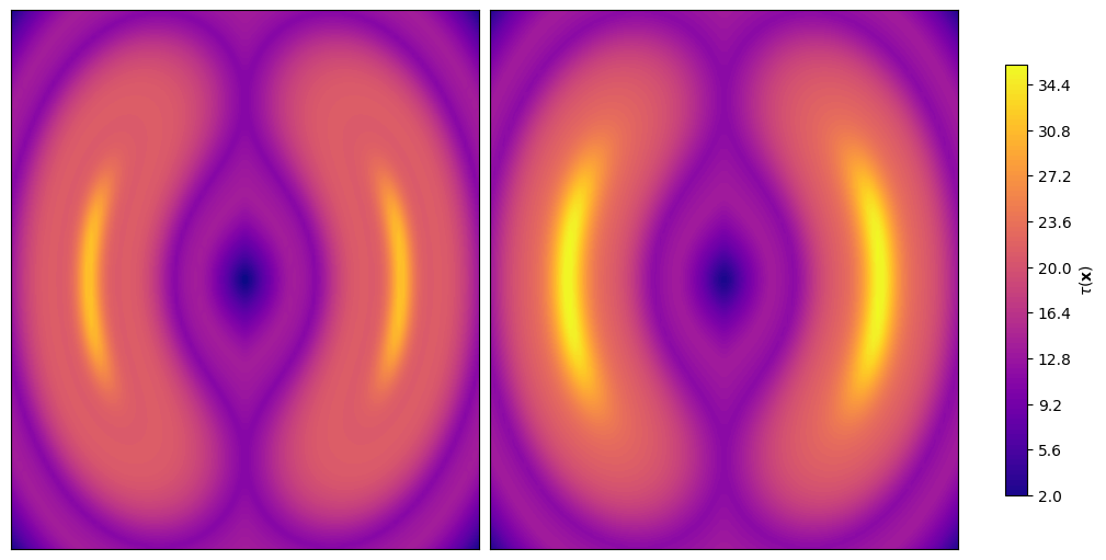
Figure A.0: Illustration of the tempering fields under two different RUMs when $p$ is Twomoons2D (Stimper et al., 2022). The tempering field $\tau(\mathbf{x})$ of the exponential RUM (left, Theorem A.1) and the Bradley-Terry model (right, Theorem 3.1).

Appendix B Proofs

Theorem A.1.

Assume $W\sim\text{Exp}(s)$. A tempering field $\tau(\mathbf{x})$ exists between the belief density $p$ and the MWD $p_{w}$, and it is given by the formula,

$$\tau(\mathbf{x})=\frac{1}{s}\left(\frac{2vol(L_{\mathbf{x}})+2p^{s}(\mathbf{x})\int_{U_{\mathbf{x}}}p^{-s}(\mathbf{x}^{\prime})d\mathbf{x}^{\prime}}{p^{s}(\mathbf{x})\int_{U_{\mathbf{x}}}p^{-s}(\mathbf{x}^{\prime})d\mathbf{x}^{\prime}+p^{-s}(\mathbf{x})\int_{L_{\mathbf{x}}}p^{s}(\mathbf{x}^{\prime})d\mathbf{x}^{\prime}}-1\right),$$

where the sublevel set $L_{\mathbf{x}}=\{\mathbf{x}^{\prime}\in\mathcal{X}\mid p(\mathbf{x})\geq p(\mathbf{x}^{\prime})\}$ and the superlevel set $U_{\mathbf{x}}=\{\mathbf{x}^{\prime}\in\mathcal{X}\mid p(\mathbf{x})<p(\mathbf{x}^{\prime})\}$.

Proof.

We want to show that for each $\mathbf{x}\in\mathcal{X}$, there exists a scalar $\tau(\mathbf{x})>0$ such that $\nabla\log p(\mathbf{x})-\tau(\mathbf{x})\nabla\log p_{w}(\mathbf{x})=\mathbf{0}$. Our constructive proof determines this scalar through brute-force calculation. Fix a point $\mathbf{x}\in\mathcal{X}$, and denote a constant $\tau(\mathbf{x})=\tau>0$.

Under the exponential RUM, the MWD $p_{w}(\mathbf{x})$ equals to

$$p_{w}(\mathbf{x})=2\lambda(\mathbf{x})\int_{\mathcal{X}}F_{\text{Laplace}(0,1/s)}\left(\log p(\mathbf{x})-\log p(\mathbf{x}^{\prime})\right)\lambda(\mathbf{x}^{\prime})d\mathbf{x}^{\prime}.$$ (B.1)

For uniform $\lambda$, this implies

$$\nabla_{\mathbf{x}}\log p_{w}(\mathbf{x}) =\nabla_{\mathbf{x}}\log\int_{\mathcal{X}}F_{\text{Laplace}(0,1/s)}\left(\log p(\mathbf{x})-\log p(\mathbf{x}^{\prime})\right)d\mathbf{x}^{\prime}.$$ (B.2)

Let $L_{\mathbf{x}},U_{\mathbf{x}}\subset\mathcal{X}$ be the regions $L_{\mathbf{x}}=\{\mathbf{x}^{\prime}\in\mathcal{X}\mid p(\mathbf{x})\geq p(\mathbf{x}^{\prime})\}$ and $U_{\mathbf{x}}=\{\mathbf{x}^{\prime}\in\mathcal{X}\mid p(\mathbf{x})<p(\mathbf{x}^{\prime})\}$. Straightforward manipulations give us,

$$\tau\nabla_{\mathbf{x}}\log p_{w}(\mathbf{x})-\nabla_{\mathbf{x}}\log p(\mathbf{x})=$$

$$=\tau\nabla_{\mathbf{x}}\log\bigg(\int_{U_{\mathbf{x}}}\frac{1}{2}p^{s}(\mathbf{x})p^{-s}(\mathbf{x}^{\prime})d\mathbf{x}^{\prime}+\int_{L_{\mathbf{x}}}\left(1-\frac{1}{2}p^{-s}(\mathbf{x})p^{s}(\mathbf{x}^{\prime})\right)d\mathbf{x}^{\prime}\bigg)-\tau\nabla_{\mathbf{x}}\log p^{\frac{1}{\tau}}(\mathbf{x})$$

$$=\tau\nabla_{\mathbf{x}}\log\frac{vol(L_{\mathbf{x}})+\frac{1}{2}p^{s}(\mathbf{x})\int_{U_{\mathbf{x}}}p^{-s}(\mathbf{x}^{\prime})d\mathbf{x}^{\prime}-\frac{1}{2}p^{-s}(\mathbf{x})\int_{L_{\mathbf{x}}}p^{s}(\mathbf{x}^{\prime})d\mathbf{x}^{\prime}}{p^{\frac{1}{\tau}}(\mathbf{x})}.$$

Because $\nabla_{\mathbf{x}}\log f(\mathbf{x})=\nabla_{\mathbf{x}}f(\mathbf{x})/f(\mathbf{x})$, the above vanishes, if and only if,

$$\nabla_{\mathbf{x}}\left(p^{-\frac{1}{\tau}}(\mathbf{x})vol(L_{\mathbf{x}})+\frac{1}{2}p^{s-\frac{1}{\tau}}(\mathbf{x})\int_{U_{\mathbf{x}}}p^{-s}(\mathbf{x}^{\prime})d\mathbf{x}^{\prime}-\frac{1}{2}p^{-s-\frac{1}{\tau}}(\mathbf{x})\int_{L_{\mathbf{x}}}p^{s}(\mathbf{x}^{\prime})d\mathbf{x}^{\prime}\right)=\mathbf{0}.$$

We will apply to LHS the generalized Leibniz integral rule (Flanders, 1973) for each fixed dimension $j\in\{1,...,d\}$ by interpreting $\frac{\partial}{\partial\mathbf{x}_{j}}$ as differentiation with respect to the time. To justify the generalized Leibniz integral rule, note that the boundaries $\partial L_{\mathbf{x}}=\partial U_{\mathbf{x}}$ are defined by an implicit function $g:\mathcal{X}\rightarrow\mathcal{X}$ whose graph is the set $\{(\mathbf{x},g(\mathbf{x}))\}=\{(\mathbf{x},\mathbf{x}^{\prime})\in\mathcal{X}^{2}\mid f(\mathbf{x},\mathbf{x}^{\prime})=0\}$, where the function $f(\mathbf{x},\mathbf{x}^{\prime}):=p(\mathbf{x})-p(\mathbf{x}^{\prime})$ is continuously differentiable by Assumption 3. Moreover, since $\nabla_{\mathbf{x}^{\prime}}f(\mathbf{x},\mathbf{x}^{\prime})=-\nabla p(\mathbf{x}^{\prime})\neq 0$ almost everywhere, the implicit function theorem implies that the level set $\{(\mathbf{x},\mathbf{x}^{\prime})\mid f(\mathbf{x},\mathbf{x}^{\prime})=0\}$ locally defines $\mathbf{x}^{\prime}$ as a differentiable function of $\mathbf{x}$ almost everywhere. Therefore, $g(\mathbf{x})$ is continuously differentiable almost everywhere.

For a smooth function $f:\mathcal{X}\rightarrow\mathbb{R}_{+}$ consider,

$$\frac{\partial}{\partial\mathbf{x}_{j}}\int_{A_{\mathbf{x}}}f(\mathbf{x}^{\prime})d\mathbf{x}^{\prime},$$

where $A_{\mathbf{x}}=L_{\mathbf{x}}$ or $A_{\mathbf{x}}=U_{\mathbf{x}}$. Interpret the scalar $\mathbf{x}_{j}$ as time, and apply the generalized Leibniz integral rule,

$$\frac{\partial}{\partial\mathbf{x}_{j}}\int_{A_{\mathbf{x}}}f(\mathbf{x}^{\prime})d\mathbf{x}^{\prime}=\int_{A_{\mathbf{x}}}\frac{\partial}{\partial\mathbf{x}_{j}}f(\mathbf{x}^{\prime})d\mathbf{x}^{\prime}+\int_{\partial A_{\mathbf{x}}}f(\mathbf{x}^{\prime})(\mathbf{n}\cdot\mathbf{v})dS,$$

where $\mathbf{n}$ is the unit normal vector pointing outwards from the boundary $\partial A_{\mathbf{x}}$, $\mathbf{v}$ is the Eulerian velocity of the boundary $\partial A_{\mathbf{x}}$ when $\mathbf{x}_{j}$ is interpreted as time, and $dS$ is the surface element. The first term in RHS vanishes. For the second term, consider the level set $\{\mathbf{x}^{\prime}\in\mathcal{X}\mid p(\mathbf{x})-p(\mathbf{x}^{\prime})=0\}$. The normal vector is orthogonal to this level set, which equals to gradient with respect to $\mathbf{x}^{\prime}$, $\mathbf{n}=\nabla_{\mathbf{x}^{\prime}}(p(\mathbf{x})-p(\mathbf{x}^{\prime}))/\left\lVert\nabla_{\mathbf{x}^{\prime}}(p(\mathbf{x})-p(\mathbf{x}^{\prime}))\right\rVert=-\nabla_{\mathbf{x}^{\prime}}p(\mathbf{x}^{\prime})/\left\lVert\nabla_{\mathbf{x}^{\prime}}p(\mathbf{x}^{\prime})\right\rVert$. This corresponds to the normal vector of $L_{\mathbf{x}}$ while the normal vector of $U_{\mathbf{x}}$ is with the opposite sign.

Let us consider $\mathbf{v}=(\frac{\partial\mathbf{x}_{1}^{\prime}}{\partial\mathbf{x}_{j}},...,\frac{\partial\mathbf{x}_{N}^{\prime}}{\partial\mathbf{x}_{j}})$, the velocity of the boundary with respect to $\mathbf{x}_{j}$. The total derivative of the boundary should not change,

$$D_{\mathbf{x}_{j}}(p(\mathbf{x})-p(\mathbf{x}^{\prime}))=0$$

$$\frac{\partial}{\partial\mathbf{x}_{j}}(p(\mathbf{x})-p(\mathbf{x}^{\prime}))+\sum_{i=1}^{d}\frac{\partial}{\partial\mathbf{x}_{i}^{\prime}}(p(\mathbf{x})-p(\mathbf{x}^{\prime}))\frac{\partial\mathbf{x}_{i}^{\prime}}{\partial\mathbf{x}_{j}}=0$$

$$\frac{\partial}{\partial\mathbf{x}_{j}}p(\mathbf{x})-\sum_{i=1}^{d}\frac{\partial}{\partial\mathbf{x}_{i}^{\prime}}p(\mathbf{x}^{\prime})\frac{\partial\mathbf{x}_{i}^{\prime}}{\partial\mathbf{x}_{j}}=0.$$

Taking the dot product of the constraint with the normal vector gives,

$$\mathbf{n}\cdot\mathbf{v} =-\frac{\frac{\partial}{\partial\mathbf{x}_{j}}p(\mathbf{x})}{\left\lVert\nabla_{\mathbf{x}^{\prime}}p(\mathbf{x}^{\prime})\right\rVert}.$$

Since $p(\mathbf{x}^{\prime})=p(\mathbf{x})$ on $\partial L_{\mathbf{x}}=\partial U_{\mathbf{x}}$,

$$\frac{\partial}{\partial\mathbf{x}_{j}}\int_{L_{\mathbf{x}}}p^{s}(\mathbf{x}^{\prime})d\mathbf{x}^{\prime} =-p^{s}(\mathbf{x})\frac{\partial}{\partial\mathbf{x}_{j}}p(\mathbf{x})\int_{\partial L_{\mathbf{x}}}\frac{1}{\left\lVert\nabla_{\mathbf{x}^{\prime}}p(\mathbf{x}^{\prime})\right\rVert}dS(\mathbf{x}^{\prime})$$

$$\frac{\partial}{\partial\mathbf{x}_{j}}\int_{U_{\mathbf{x}}}p^{-s}(\mathbf{x}^{\prime})d\mathbf{x}^{\prime} =p^{-s}(\mathbf{x})\frac{\partial}{\partial\mathbf{x}_{j}}p(\mathbf{x})\int_{\partial L_{\mathbf{x}}}\frac{1}{\left\lVert\nabla_{\mathbf{x}^{\prime}}p(\mathbf{x}^{\prime})\right\rVert}dS(\mathbf{x}^{\prime})$$

$$\frac{\partial}{\partial\mathbf{x}_{j}}\int_{L_{\mathbf{x}}}d\mathbf{x}^{\prime} =-\frac{\partial}{\partial\mathbf{x}_{j}}p(\mathbf{x})\int_{\partial L_{\mathbf{x}}}\frac{1}{\left\lVert\nabla_{\mathbf{x}^{\prime}}p(\mathbf{x}^{\prime})\right\rVert}dS(\mathbf{x}^{\prime}).$$

Together these imply that,

$$\left(p^{-\frac{1}{\tau}}(\mathbf{x})\frac{\partial}{\partial\mathbf{x}_{j}}\int_{L_{\mathbf{x}}}d\mathbf{x}^{\prime}+\frac{1}{2}p^{s-\frac{1}{\tau}}(\mathbf{x})\frac{\partial}{\partial\mathbf{x}_{j}}\int_{U_{\mathbf{x}}}p^{-s}(\mathbf{x}^{\prime})d\mathbf{x}^{\prime}-\frac{1}{2}p^{-s-\frac{1}{\tau}}(\mathbf{x})\frac{\partial}{\partial\mathbf{x}_{j}}\int_{L_{\mathbf{x}}}p^{s}(\mathbf{x}^{\prime})d\mathbf{x}^{\prime}\right)=0.$$

We are left with the following terms that vanish,

$$p^{-\frac{1}{\tau}-1}(\mathbf{x})\nabla_{\mathbf{x}}p(\mathbf{x})\left(-\frac{1}{\tau}vol(L_{\mathbf{x}})+\frac{s-\frac{1}{\tau}}{2}p^{s}(\mathbf{x})\int_{U_{\mathbf{x}}}p^{-s}(\mathbf{x}^{\prime})d\mathbf{x}^{\prime}+\frac{s+\frac{1}{\tau}}{2}p^{-s}(\mathbf{x})\int_{L_{\mathbf{x}}}p^{s}(\mathbf{x}^{\prime})d\mathbf{x}^{\prime}\right).$$

In order to this hold, the scalar in the parenthesis must vanish,

$$\frac{2}{\tau}vol(L_{\mathbf{x}})+\frac{1}{\tau}p^{s}(\mathbf{x})\int_{U_{\mathbf{x}}}p^{-s}(\mathbf{x}^{\prime})d\mathbf{x}^{\prime}-\frac{1}{\tau}p^{-s}(\mathbf{x})\int_{L_{\mathbf{x}}}p^{s}(\mathbf{x}^{\prime})d\mathbf{x}^{\prime}$$

$$=sp^{s}(\mathbf{x})\int_{U_{\mathbf{x}}}p^{-s}(\mathbf{x}^{\prime})d\mathbf{x}^{\prime}+sp^{-s}(\mathbf{x})\int_{L_{\mathbf{x}}}p^{s}(\mathbf{x}^{\prime})d\mathbf{x}^{\prime}.$$

Rearranging the terms give us,

$$\tau=\frac{1}{s}\left(\frac{2vol(L_{\mathbf{x}})+2p^{s}(\mathbf{x})\int_{U_{\mathbf{x}}}p^{-s}(\mathbf{x}^{\prime})d\mathbf{x}^{\prime}}{p^{s}(\mathbf{x})\int_{U_{\mathbf{x}}}p^{-s}(\mathbf{x}^{\prime})d\mathbf{x}^{\prime}+p^{-s}(\mathbf{x})\int_{L_{\mathbf{x}}}p^{s}(\mathbf{x}^{\prime})d\mathbf{x}^{\prime}}-1\right).$$

∎

Theorem 3.1.

Assume $W\sim\text{Gumbel}(0,s)$. A tempering field $\tau(\mathbf{x})$ exists between the belief density $p$ and the MWD $p_{w}$, and it is given by the formula,

$$\tau(\mathbf{x})=s\left(\frac{\int_{\mathcal{X}}\frac{1}{1+r_{s}(\mathbf{x},\mathbf{x}^{\prime})}d\mathbf{x}^{\prime}}{\int_{\mathcal{X}}\frac{r_{s}(\mathbf{x},\mathbf{x}^{\prime})}{(1+r_{s}(\mathbf{x},\mathbf{x}^{\prime}))^{2}}d\mathbf{x}^{\prime}}\right),$$ (B.3)

where $r_{s}(\mathbf{x},\mathbf{x}^{\prime}):=p^{\frac{1}{s}}(\mathbf{x}^{\prime})p^{-\frac{1}{s}}(\mathbf{x})$ is $1/s$-tempered density ratio.

Proof.

Under the Bradley-Terry model, $W\sim\text{Gumbel}(0,s)$, and the MWD $p_{w}(\mathbf{x})$ now equals to

$$p_{w}(\mathbf{x})=2\lambda(\mathbf{x})\int_{\mathcal{X}}F_{\text{Logistic}(0,s)}\left(\log p(\mathbf{x})-\log p(\mathbf{x}^{\prime})\right)\lambda(\mathbf{x}^{\prime})d\mathbf{x}^{\prime}.$$ (B.4)

Following same lines of reasoning as in the constructive proof of Theorem A.1, we fix $\mathbf{x}\in\mathcal{X}$ and aim to find a constant $\tau(\mathbf{x})=\tau>0$ solving the tempering field condition. Unless $p$ is uniform, the necessary and sufficient condition for the existence of $\tau$ is that it solves the equation,

$$p^{-1-\frac{1}{\tau}}(\mathbf{x})\int_{\mathcal{X}}\frac{\frac{1}{s}p^{-\frac{1}{s}}(\mathbf{x})p^{\frac{1}{s}}(\mathbf{x}^{\prime})-\frac{1}{\tau}\left(1+p^{-\frac{1}{s}}(\mathbf{x})p^{\frac{1}{s}}(\mathbf{x}^{\prime})\right)}{\left(1+p^{-\frac{1}{s}}(\mathbf{x})p^{\frac{1}{s}}(\mathbf{x}^{\prime})\right)^{2}}d\mathbf{x}^{\prime}=0.$$

This is equivalent to,

$$\tau=s\left(\frac{\int_{\mathcal{X}}\frac{1}{1+r_{s}(\mathbf{x},\mathbf{x}^{\prime})}d\mathbf{x}^{\prime}}{\int_{\mathcal{X}}\frac{r_{s}(\mathbf{x},\mathbf{x}^{\prime})}{(1+r_{s}(\mathbf{x},\mathbf{x}^{\prime}))^{2}}d\mathbf{x}^{\prime}}\right),$$ (B.5)

where for clarity we denote $r_{s}(\mathbf{x},\mathbf{x}^{\prime}):=p^{\frac{1}{s}}(\mathbf{x}^{\prime})p^{-\frac{1}{s}}(\mathbf{x})=\left(\frac{p(\mathbf{x}^{\prime})}{p(\mathbf{x})}\right)^{1/s}$, which is $1/s$-tempered density ratio between density values at compared points $\mathbf{x}^{\prime}$ and $\mathbf{x}$. ∎

Proposition 3.2.

Assume that there exists a tempering field $\tau(\mathbf{x})$ between $p$ and $q$. A tempering parameter $\tau^{\star}>0$ defined by,

$$\tau^{\star}=\mathbb{E}_{X\sim p}\left(\omega(X)\tau(X)\right),$$ (B.6)

where a stochastic weight $\omega\geq 0$ is given by

$$\omega(X)=\frac{\left\lVert\nabla\log q(X)\right\rVert^{2}}{\mathbb{E}_{X\sim p}\left(\left\lVert\nabla\log q(X)\right\rVert^{2}\right)},$$

minimizes the Fisher divergence between $p$ and $q$,

$$\tau^{\star}=\operatorname*{arg\,min}_{\tau>0}F(p,q^{\tau}).$$ (B.7)

Proof.

By the Leibniz formula,

$$\frac{\partial}{\partial\tau}\int_{\mathcal{X}}\left\lVert\nabla_{\mathbf{x}}\log q^{\tau}(\mathbf{x})-\nabla_{\mathbf{x}}\log p(\mathbf{x})\right\rVert^{2}p(\mathbf{x})d\mathbf{x}$$

$$=\int_{\mathcal{X}}\frac{\partial}{\partial\tau}\left\lVert\nabla_{\mathbf{x}}\log q^{\tau}(\mathbf{x})-\nabla_{\mathbf{x}}\log p(\mathbf{x})\right\rVert^{2}p(\mathbf{x})d\mathbf{x}$$

$$=\int_{\mathcal{X}}2\left(\tau\left\lVert\nabla_{\mathbf{x}}\log q(\mathbf{x})\right\rVert^{2}-\langle\nabla_{\mathbf{x}}\log q(\mathbf{x}),\nabla_{\mathbf{x}}\log p(\mathbf{x})\rangle\right)p(\mathbf{x})d\mathbf{x}.$$

Since the Fisher score is quadratic in $\tau$, the critical point corresponds to the global minimum. By the assumption, $\langle\nabla_{\mathbf{x}}\log q(\mathbf{x}),\nabla_{\mathbf{x}}\log p(\mathbf{x})\rangle=\tau(\mathbf{x})\left\lVert\nabla_{\mathbf{x}}\log q(\mathbf{x})\right\rVert^{2}$. Hence,

$$\tau^{\star}=\frac{\mathbb{E}_{X\sim p}\left(\tau(X)\left\lVert\nabla\log q(X)\right\rVert^{2}\right)}{\mathbb{E}_{X\sim p}\left(\left\lVert\nabla\log q(X)\right\rVert^{2}\right)}.$$

∎

Lemma B.4.

Let $\tau(\mathbf{x})$ be a tempering field. For any $\tau>0$ it holds that

$$F(p,q^{\tau})=\int_{\mathcal{X}}|\tau-\tau(\mathbf{x})|^{2}\left\lVert\nabla_{\mathbf{x}}\log q(\mathbf{x})\right\rVert^{2}p(\mathbf{x})d\mathbf{x}.$$

Proof.

Since $\tau(\mathbf{x})$ is a tempering field,

$$\left\lVert\nabla_{\mathbf{x}}\log q^{\tau}(\mathbf{x})-\nabla_{\mathbf{x}}\log p(\mathbf{x})\right\rVert$$

$$=\left\lVert(\tau-\tau(\mathbf{x}))\nabla_{\mathbf{x}}\log q(\mathbf{x})+(\tau(\mathbf{x})\nabla_{\mathbf{x}}\log q(\mathbf{x})-\nabla_{\mathbf{x}}\log p(\mathbf{x}))\right\rVert$$

$$=\left\lVert(\tau-\tau(\mathbf{x}))\nabla_{\mathbf{x}}\log q(\mathbf{x})\right\rVert.$$

∎

Proposition B.5.

Let $\tau^{\star}$ be the optimal tempering and $\tau(\mathbf{x})$ a tempering field.

$$F(p,q^{\tau^{\star}})=\mathbb{E}\left(\left\lVert\nabla\log q(X)\right\rVert^{2}\tau^{2}(X)\right)-\frac{\left(\mathbb{E}\left(\tau(X)\left\lVert\nabla\log q(X)\right\rVert^{2}\right)\right)^{2}}{\mathbb{E}\left(\left\lVert\nabla\log q(X)\right\rVert^{2}\right)}.$$

Proof.

By Proposition 3.2 and Lemma B.4,

$$\int_{\mathcal{X}}\left\lVert\nabla_{\mathbf{x}}\log q^{\tau^{\star}}(\mathbf{x})-\nabla_{\mathbf{x}}\log p(\mathbf{x})\right\rVert^{2}p(\mathbf{x})d\mathbf{x}$$

$$=\mathbb{E}\left(|\tau^{\star}-\tau(X)|^{2}\left\lVert\nabla\log q(X)\right\rVert^{2}\right)$$

$$=\mathbb{E}\left(\left(\frac{\mathbb{E}\left(\tau(X^{\prime})\left\lVert\nabla\log q(X^{\prime})\right\rVert^{2}\right)}{\mathbb{E}\left(\left\lVert\nabla\log q(X^{\prime})\right\rVert^{2}\right)}-\tau(X)\right)^{2}\left\lVert\nabla\log q(X)\right\rVert^{2}\right)$$

$$=\mathbb{E}\left(\left(\frac{\left\lVert\nabla\log q(X)\right\rVert\mathbb{E}\left(\tau(X^{\prime})\left\lVert\nabla\log q(X^{\prime})\right\rVert^{2}\right)}{\mathbb{E}\left(\left\lVert\nabla\log q(X^{\prime})\right\rVert^{2}\right)}-\left\lVert\nabla\log q(X)\right\rVert\tau(X)\right)^{2}\right)$$

$$=\frac{\left(\mathbb{E}\left(\tau(X)\left\lVert\nabla\log q(X)\right\rVert^{2}\right)\right)^{2}}{\mathbb{E}\left(\left\lVert\nabla\log q(X)\right\rVert^{2}\right)}-2\frac{\left(\mathbb{E}\left(\tau(X)\left\lVert\nabla\log q(X)\right\rVert^{2}\right)\right)^{2}}{\mathbb{E}\left(\left\lVert\nabla\log q(X)\right\rVert^{2}\right)}+\mathbb{E}\left(\left\lVert\nabla\log q(X)\right\rVert^{2}\tau^{2}(X)\right)$$

$$=\mathbb{E}\left(\left\lVert\nabla\log q(X)\right\rVert^{2}\tau^{2}(X)\right)-\frac{\left(\mathbb{E}\left(\tau(X)\left\lVert\nabla\log q(X)\right\rVert^{2}\right)\right)^{2}}{\mathbb{E}\left(\left\lVert\nabla\log q(X)\right\rVert^{2}\right)}.$$

∎

Proposition 3.3.

Let $\tau(\mathbf{x})$ be a tempering field. For any $\tau>0$ it holds that

$$F(p,q^{\tau})=\mathbb{E}_{X\sim p}\left(|\tau-\tau(X)|^{2}\left\lVert\nabla\log q(X)\right\rVert^{2}\right).$$ (B.8)

Further, when $\tau^{\star}>0$ is the optimal tempering

$$F(p,q^{\tau^{\star}})=\mathbb{E}_{X\sim p}\left(\left\lVert\nabla\log q(X)\right\rVert^{2}\tau^{2}(X)\right)-\frac{\left(\mathbb{E}_{X\sim p}\left(\tau(X)\left\lVert\nabla\log q(X)\right\rVert^{2}\right)\right)^{2}}{\mathbb{E}_{X\sim p}\left(\left\lVert\nabla\log q(X)\right\rVert^{2}\right)}.$$ (B.9)

Proof.

This is a combined result of Lemma B.4 and Proposition B.5. ∎

Corollary B.7.

Assume that the expert choice model follows the Bradley-Terry model or the exponential RUM. The scores of the belief and the MWD are collinear. That is, there exists a scalar-valued function $\tau(\mathbf{x})$ such that,

$$\nabla\log p(\mathbf{x})=\tau(\mathbf{x})\nabla\log p_{w}(\mathbf{x}).$$

Proof.

Follows from the definition 6 and Theorems 3.1 and A.1. ∎

Appendix C Method

C.1 Training joint and marginals distributions

There are recent works that discuss in detail how to use diffusion model to learn between joint and arbitrary conditionals, while modeling the marginals is not always straightforward (Gloeckler et al., 2024). We adopt a simplified approach to estimate the marginal score function by leveraging a corruption-based marginalization strategy.

To model simultaneously both the joint distribution $p_{\mathbf{x}\succ\mathbf{x}^{\prime}}(\mathbf{x},\mathbf{x}^{\prime})$ and the marginal distribution $p_{w}(\mathbf{x})$, we introduce a binary conditioning variable $\mathsf{joint}\in\{\texttt{true},\texttt{false}\}$ into the score model. During training, we randomly set $\mathsf{joint}=\texttt{false}$ with 50% probability, and in this case, we mask the input $\mathbf{x}_{t}^{\prime}$ by replacing it with Gaussian noise $\mathcal{N}(\mathbf{0},\sigma_{t}^{2}\mathbf{I})$, where $\sigma_{t}$ is the current noise level. We then compute the denoising score matching loss only over the winner dimensions $\mathbf{x}$ (i.e., the first $d$ components of $\nabla\log p_{\mathbf{x}\succ\mathbf{x}^{\prime}}(\mathbf{x},\mathbf{x}^{\prime})$). When $\mathsf{joint}=\texttt{true}$, we train the model to predict the full joint score over both $\mathbf{x}$ and $\mathbf{x}^{\prime}$.

At sampling time, to generate samples from the marginal distribution $p_{w}(\mathbf{x})$ using ALD, we similarly set $\mathsf{joint}=\texttt{false}$ and replace $\mathbf{x}_{t}^{\prime}$ with Gaussian noise $\mathcal{N}(\mathbf{0},\sigma_{t}^{2}\mathbf{I})$ at each iteration of ALD. Fig. 2(a) demonstrates the benefit of training the score model on the full joint data while using the proposed marginalization method to model the marginal score.

(a) Replication of Fig. 1 using (a) only winner samples, with the score model trained only for the MWD $p_{w}(\mathbf{x})$. The quality of the final density estimate, i.e., the ‘tempered’ MWD, is clearly inferior compared to (b) training on the full joint $p_{\mathbf{x}\succ\mathbf{x}^{\prime}}(\mathbf{x},\mathbf{x}^{\prime})$ using both winners and losers.

C.2 Algorithms

Algorithm C.1 Full algorithm

 require: choice data $\mathcal{D}$

 output: samples from the belief density or a trained diffusion model for it it

 train $\mathbf{s}_{\theta}(\mathbf{x},\mathbf{x}^{\prime},\sigma,\mathsf{joint})$ using score-matching on $\mathcal{D}=\mathcal{D}_{\succ}\times\mathcal{D}_{\nsucc}$

• $50\%$ of time: set $\mathsf{joint}=0$ and mask $\mathbf{x}^{\prime}$ with $\mathcal{N}(\mathbf{0},\sigma_{t}^{2}\mathbf{I})$

• $50\%$ of time: set $\sigma$ to noise schedule $(\sigma_{t})_{t=1}^{L}$

 initialize $\tau(\mathbf{x})$ given $\mathcal{D}$ and $\mathbf{s}_{\theta}$

 sample $\mathcal{D}^{\star}$ using $\tau(\mathbf{x})$-scaled ALD with the score $\mathbf{s}_{\theta}(\mathbf{x},\mathbf{x}^{\prime},(\sigma_{t})_{t=1}^{L},\mathsf{joint}\mathord{=}0)$

  optional  

 train $\mathbf{s}_{\theta_{\text{MWD}}}(\mathbf{x},\sigma,\mathsf{temp})$ using score-matching on $\mathcal{D}^{\star}$

  

 return: $\mathcal{D}^{\star}$ or $\mathbf{s}_{\theta_{\text{MWD}}}(\mathbf{x},\sigma,\mathsf{temp}\mathord{=}1)$

Algorithm C.2 $\tau(\mathbf{x})$

 require: s, $\mathcal{D}$, $\mathbf{s}_{\theta}$

 initialize:

• train $r_{\theta}(\mathbf{x},\mathbf{x}^{\prime})\approx\frac{p(\mathbf{x}^{\prime})}{p(\mathbf{x})}$ as MLE of $\mathcal{D}$ (binary cross-entropy loss)

• sample $m$ points $\mathbf{X}$ with densities $p_{w}(\mathbf{X})$ using $\mathbf{s}_{\theta}$ (Appendix C.8)

 input: $\mathbf{x}$

 $\mathbf{r}=(r_{\theta}(\mathbf{x},\mathbf{X}))^{\frac{1}{s}}$

 return: $s\left(\frac{\sum_{i=1}^{m}\frac{1}{1+\mathbf{r}_{i}}\frac{1}{p_{w}(\mathbf{X}_{i})}}{\sum_{i=1}^{m}\frac{\mathbf{r}_{i}}{(1+\mathbf{r}_{i})^{2}}\frac{1}{p_{w}(\mathbf{X}_{i})}}\right)$

C.3 Details on modeling the ‘tempered’ MWD

To learn the MWD $p_{w}(\mathbf{x})$, having only access to samples from the joint distribution of winners and losers $p_{\mathbf{x}\succ\mathbf{x}^{\prime}}(\mathbf{x},\mathbf{x}^{\prime})$, we propose learning the full joint and the first marginal to capture the preference relationships in the data while enabling sampling from the tempered marginal via score-scaled ALD. To that end, we parametrize the score model $\mathbf{s}_{\theta}(\mathbf{x},\mathbf{x}^{\prime},\sigma,\mathsf{joint},\mathsf{temp})$ such that $(\mathbf{x},\mathbf{x}^{\prime})\mapsto\mathbf{s}_{\theta}(\mathbf{x},\mathbf{x}^{\prime},\sigma_{\min},\mathsf{joint}\mathord{=}1,\mathsf{temp}\mathord{=}0)$ models the score of the joint distribution of winners and losers, i.e., $\nabla\log p_{\mathbf{x}\succ\mathbf{x}^{\prime}}(\mathbf{x},\mathbf{x}^{\prime})$, and $(\mathbf{x},\mathsf{temp})\mapsto\mathbf{s}_{\theta}(\mathbf{x},\emptyset,\sigma_{\min},\mathsf{joint}\mathord{=}0,\mathsf{temp})$ models the score of the MWD and its ‘tempered’ version, i.e., $\nabla\log p_{w}(\mathbf{x})$ and $\tau(\mathbf{x})\nabla\log p_{w}(\mathbf{x})$, respectively. This allows training the score network with both winners and losers, while still enabling sampling from the belief density via the approximation $\mathbf{s}_{\theta}(\mathbf{x},\emptyset,\sigma_{\min},\mathsf{joint}\mathord{=}0,\mathsf{temp}\mathord{=}1)\approx\tau(\mathbf{x})\nabla\log p_{w}(\mathbf{x})=\nabla\log p(\mathbf{x})$. Fig. 2(a) validates that the joint score model is superior to directly learning the marginal from only the winner samples.

We implement the method by training a score model through the denoising score matching equation 1 on the concatenation of winners and losers, with random masking of losers during training (for more details, see Appendix C.1). Technically speaking, to enable sampling via reverse diffusion and ALD, we use a noise distribution $p_{\text{train}}(\sigma)$ during training, defined as a mixture of a Dirac delta on a cosine noise schedule and a $\mathrm{LogNormal}(P_{\text{mean}},P_{\text{std}}^{2})$, with mixture weight $\phi=0.5$ assigned to the Dirac delta component. We stay as close as possible to the EDM-style diffusion model (Karras et al., 2024a). Specifically, we use the perturbation kernel $p_{\sigma}(\tilde{\mathbf{x}}|\mathbf{x})=\mathcal{N}(\tilde{\mathbf{x}};\mathbf{x},\sigma^{2}\mathbf{I})$, which aligns with EDM and defines a forward diffusion process from $\sigma_{\min}$ to $\sigma_{\max}$, where $p_{\sigma_{\min}}(\mathbf{x})\approx p(\mathbf{x})$ and $p_{\sigma_{\max}}(\mathbf{x})\approx\mathcal{N}(\mathbf{0},\sigma_{\max}^{2}\mathbf{I})$. After training $\mathbf{s}_{\theta}(\mathbf{x},\mathbf{x}^{\prime},\sigma,\mathsf{joint},0)$ on perturbed winners and losers, we sample from the belief density using the score-scaled ALD. We can either stop here, or optionally train the tempered marginal score network $\mathbf{s}_{\theta_{\text{MWD}}}(\mathbf{x},\sigma,\mathsf{temp})$, which weights can be initialized to that of $\mathbf{s}_{\theta}$, through denoising score matching using the sampled data. Finally, we use the loss weighting $\ell(\sigma)=\sigma^{2}$. Algorithms C.1–C.2 summarize the method.

C.4 Score model

We follow as closely as possible the EDM2 specifications used in the 2D toy experiment in (Karras et al., 2024a). For both the joint score network and the tempered MWD score network, we use an MLP with one input layer and four hidden layers, SiLU activation functions (Hendrycks & Gimpel, 2016) are applied after each hidden layer, and implemented using the magnitude-preserving primitives from EDM2 (Karras et al., 2024b). In the joint score network, the input is a $(2d+3)$-dimensional vector $(x,x^{\prime},\sigma,\mathsf{joint},\mathsf{temp})$, and the output of each hidden layer has $h$ features, where $h\in\{32,64,96,128\}$ depending on the experiment dimensionality. In the MWD score network, the input is a $(d+3)$-dimensional vector $(x,\sigma,0,\mathsf{temp})$. The binary variables $\mathsf{joint}$ and $\mathsf{temp}$ are linearly embedded into an $h/4$-dimensional space. Further, a simple residual connection is applied to the embedded variables through all hidden layers. Otherwise, we use the same preconditioning for the score network as described in EDM (Karras et al., 2022).

C.5 Belief density ratio model

We parametrize the belief density ratio $r_{\theta}(\mathbf{x},\mathbf{x}^{\prime})\approx p(\mathbf{x}^{\prime})/p(\mathbf{x})$ via parameterizing the unnormalized log density $f_{\theta}(\mathbf{x})\approx\log p(\mathbf{x})+constant$ as an MLP with three hidden layers with SiLu activations, and one output layer, such that $\log r_{\theta}(\mathbf{x},\mathbf{x}^{\prime})=f_{\theta}(\mathbf{x}^{\prime})-f_{\theta}(\mathbf{x})$. The number of hidden units is tied to that of the score model (Section C.4). Regularization of the weights $\theta$ is important for obtaining sensible results. To this end, we apply adaptive $\ell_{2}$-regularization using the Adam optimizer (Kingma & Ba, 2015) with weight decay. In contrast, standard $\ell_{2}$-regularization, corresponding to AdamW (Loshchilov & Hutter, 2019), yielded slightly inferior empirical performance. We set the weight decay to $10^{-3}$, except in the small data $n=100d$ experiments, where we use a higher value of $3\times 10^{-3}$.

C.6 Tempering field estimate

For the $d$-dimensional target, we use $2000d$ importance samples to estimate the integrals in the tempering field formula 7. The importance weights are computed using the probability ODE of the MWD diffusion model (see Appendix C.8 for details). The estimated tempering field $\tau(\mathbf{x})$ is clipped such that $1\leq\tau(\mathbf{x})\leq Q_{\tau}(0.999)$, where $Q_{\tau}(0.999)$ denotes the $99.9\%$ quantile of the estimated tempering field values. The lower bound follows directly from the theory (i.e., from formula 7), while the upper bound is introduced for numerical stability to remove outliers.

C.7 Score-scaled ALD

Score-scaled ALD uses the scaled score $\tau(\mathbf{x})\nabla\log p_{w}(\mathbf{x})$, where $\nabla\log p_{w}(\mathbf{x})$ is replaced by our estimated score. While $\tau(\mathbf{x})$ is not the ALD step size $\epsilon>0$, it is clear that $\tau(\mathbf{x})$ influences the ALD update in a manner similar to $\epsilon$. To ensure convergence of score-scaled ALD, at each ALD step we use the step size $\epsilon=\frac{\epsilon_{\text{base}}}{\tau(\mathbf{x})}\frac{\sigma^{2}}{\sigma_{\max}^{2}}$, where $\epsilon_{\text{base}}$ is the base step size to be specified. The required number of iterations $T$ should be chosen with respect to $\epsilon_{\text{base}}$. In our experiments, we use $L=50$, $T=40$, and $\epsilon_{\text{base}}=0.15$. In $2D$-experiments, we use faster sampling parameters: $L=15$, $T=40$, and $\epsilon_{\text{base}}=7.0$. Regarding the injection of a deterministic ALD noise schedule during denoising score-matching training, we find that the cosine schedule yields better empirical performance, while the noise schedule corresponding to the EDM time-step discretization is also a natural option.

C.8 Density evaluation of a diffusion model

Chen et al. (2018) showed that for a random variable whose probability density evolves over time, with dynamics $d\mathbf{x}=\tilde{f}(\mathbf{x}_{t},t)\,dt$ (where $\tilde{f}$ is Lipschitz continuous in $\mathbf{x}$ and continuous in $t$), the log-density at a point $\mathbf{x}_{0}$ is given by

$$\log p_{0}(\mathbf{x}_{0})=\log p_{T}(\mathbf{x}_{T})+\int_{0}^{T}\nabla\cdot\tilde{f}(\mathbf{x}_{t},t)\,dt,$$ (C.1)

where $\nabla\cdot$ denotes the divergence operator, which is equal to the trace of the Jacobian. In practice, the divergence is often approximated using the Skilling–Hutchinson trace estimator (Grathwohl et al., 2019),

$$\nabla\cdot\tilde{f}(\mathbf{x})\approx\mathbb{E}_{\bm{\epsilon}\sim\mathcal{N}(\mathbf{0},\mathbf{I})}[\bm{\epsilon}^{\intercal}J_{\tilde{f}}(\mathbf{x})\bm{\epsilon}],$$

where the expectation is estimated using a finite number of samples.

Now, applying this to EDM-type diffusion model, which is characterized by the probability ODE

$$d\mathbf{x}=-\sigma\nabla\log p_{\sigma}(\mathbf{x})\,d\sigma,$$ (C.2)

we can compute the probability density at a point $\mathbf{x}$ as

$$\log p(\mathbf{x})\approx\log\mathcal{N}(\mathbf{x}_{\sigma_{\text{max}}};\mathbf{0},\sigma_{\text{max}}\mathbf{I})-\int_{\sigma_{\text{min}}}^{\sigma_{\text{max}}}\sigma\nabla\cdot\nabla\log p_{\sigma}(\mathbf{x}_{\sigma})\,d\sigma,$$ (C.3)

where the score $\nabla\log p_{\sigma}(\mathbf{x})$ is approximated by the score network $s_{\theta}(\mathbf{x},\sigma)$, and the divergence term is estimated using the Skilling–Hutchinson estimator.

Finally, note that the ODE in Eq. C.2 is typically stiff, requiring a careful choice of numerical integration method for stable results. Choosing an appropriate integration scheme is crucial for robust and accurate performance in our setup, as the approximation error of the score network (due to limited data) can be larger than in typical setups. To integrate Eq. C.3, we solve the coupled system

$$\frac{d\mathbf{x}}{d\sigma}=-\sigma\,s_{\theta}(\mathbf{x},\sigma),\qquad\frac{d\log p(\mathbf{x})}{d\sigma}=\sigma\,\nabla\cdot s_{\theta}(\mathbf{x},\sigma),$$

where the latter ODE tracks the accumulation of the log-density. To solve the coupled system, we use the implicit Adams–Bashforth–Moulton black-box ODE solver implemented in the torchdiffeq package (Chen, 2018).

Appendix D RUM under the space reparametrization

This appendix studies the exponential RUM and the Bradley–Terry model under space reparametrization, and verifies that both RUMs are invariant under this transformation. This justifies our approach of transforming possible non-uniform $\lambda(\mathbf{x})$ into a uniform distribution.

The winner densities of the exponential RUM and the Bradley-Terry model can be written

$$p_{w}(\mathbf{x})=2\lambda(\mathbf{x})\int_{\mathcal{X}}F_{\text{Laplace}(0,1/s)}\left(\log p(\mathbf{x})-\log p(\mathbf{x}^{\prime})\right)\lambda(\mathbf{x}^{\prime})d\mathbf{x}^{\prime},$$

and

$$p_{w}(\mathbf{x})=2\lambda(\mathbf{x})\int_{\mathcal{X}}F_{\text{Logistic}(0,s)}\left(\log p(\mathbf{x})-\log p(\mathbf{x}^{\prime})\right)\lambda(\mathbf{x}^{\prime})d\mathbf{x}^{\prime},$$

respectively. Let $d=1$. Denote the cumulative distribution function of $\lambda$ as $Q$. By the $1d$ probability change of variable formula, the winner densities in the re-parametrized space $\mathbf{x}\mapsto Q(\mathbf{x})$ can be written

$$p_{w}(\mathbf{x})=\left|\frac{d}{d\mathbf{x}}Q^{-1}(\mathbf{x})\right|\left(2q(Q^{-1}(\mathbf{x}))\int_{\mathcal{X}}F_{\text{Laplace}(0,1/s)}\left(\log p(Q^{-1}(\mathbf{x}))-\log p(\mathbf{x}^{\prime})\right)\lambda(\mathbf{x}^{\prime})d\mathbf{x}^{\prime}\right),$$

and

$$p_{w}(\mathbf{x})=\left|\frac{d}{d\mathbf{x}}Q^{-1}(\mathbf{x})\right|\left(2q(Q^{-1}(\mathbf{x}))\int_{\mathcal{X}}F_{\text{Logistic}(0,s)}\left(\log p(Q^{-1}(\mathbf{x}))-\log p(\mathbf{x}^{\prime})\right)\lambda(\mathbf{x}^{\prime})d\mathbf{x}^{\prime}\right),$$

respectively. The volume change $\left|\frac{d}{d\mathbf{x}}Q^{-1}(\mathbf{x})\right|=1/q(Q^{-1}(\mathbf{x}))$. Similarly, applying the integration by substitution formula to the transformation $\mathbf{x}^{\prime}\mapsto Q^{-1}(\mathbf{x}^{\prime})$ with the volume change $\left|\frac{d}{d\mathbf{x}^{\prime}}Q^{-1}(\mathbf{x}^{\prime})\right|$. Hence,

$$p_{w}(\mathbf{x})=2\int_{\mathcal{X}_{trans}}F_{\text{Laplace}(0,1/s)}\left(\log p(Q^{-1}(\mathbf{x}))-\log p(Q^{-1}(\mathbf{x}^{\prime}))\right)d\mathbf{x}^{\prime},$$

and

$$p_{w}(\mathbf{x})=2\int_{\mathcal{X}_{trans}}F_{\text{Logistic}(0,s)}\left(\log p(Q^{-1}(\mathbf{x}))-\log p(Q^{-1}(\mathbf{x}^{\prime}))\right)d\mathbf{x}^{\prime},$$

respectively, where $\mathcal{X}_{trans}$ is the transformed space, i.e. the hypercube. We can define the belief density in the transformed space as $p_{trans}(\mathbf{x})=p(Q^{-1}(\mathbf{x}))$. Hence, the RUM in the transformed space is the same as in the original space but with uniform sampling distribution and the utility function $\log p_{trans}(\mathbf{x})=\log p(Q^{-1}(\mathbf{x}))$.

Appendix E Experimental details

E.1 Target distributions

The log unnormalized densities of the target distributions used in the synthetic experiments are provided below.

$$\textbf{Onemoon2D}:\qquad-\frac{1}{2}\left(\frac{\|\mathbf{x}\|-2}{0.2}\right)^{2}-\frac{1}{2}\left(\frac{\mathbf{x}_{1}+2}{0.3}\right)^{2}$$

$$\textbf{Twomoons2D}:-\frac{\left(\left\lVert\mathbf{x}\right\rVert-1\right)^{2}}{0.08}-\frac{\left(\left|\mathbf{x}_{1}\right|-2\right)^{2}}{0.18}+\log\left(1+e^{-\frac{4\mathbf{x}_{1}}{0.09}}\right)$$

$$\textbf{Ring2D}:\log\left(\sum_{i=1}^{k}\left(\frac{32}{\pi}e^{-32\left(\left\lVert\mathbf{x}\right\rVert-i-1\right)^{2}}\right)\right),\quad\text{where}\ k=1$$

$$\textbf{Stargaussian6D}:\qquad\log\left(\frac{1}{2}\mathcal{N}(\mathbf{x}\mid\bm{\mu},\Sigma_{1})+\frac{1}{2}\mathcal{N}(\mathbf{x}\mid\bm{\mu},\Sigma_{2})\right),\$$

$$\sigma^{2}=1,\ \rho=0.9,\ D=6,\ \bm{\mu}=3\mathbf{1}_{D},\ \Sigma_{1}=\begin{pmatrix}\sigma^{2}&\rho\sigma^{2}&\rho\sigma^{2}&\cdots&\rho\sigma^{2}\\ \rho\sigma^{2}&\sigma^{2}&\rho\sigma^{2}&\cdots&\rho\sigma^{2}\\ \rho\sigma^{2}&\rho\sigma^{2}&\sigma^{2}&\cdots&\rho\sigma^{2}\\ \vdots&\vdots&\vdots&\ddots&\vdots\\ \rho\sigma^{2}&\rho\sigma^{2}&\rho\sigma^{2}&\cdots&\sigma^{2}\end{pmatrix},$$

$$\Sigma_{2}=\begin{pmatrix}\sigma^{2}&-\rho\sigma^{2}&\rho\sigma^{2}&\cdots&(-1)^{D-1}\rho\sigma^{2}\\ -\rho\sigma^{2}&\sigma^{2}&-\rho\sigma^{2}&\cdots&(-1)^{D-2}\rho\sigma^{2}\\ \rho\sigma^{2}&-\rho\sigma^{2}&\sigma^{2}&\cdots&(-1)^{D-3}\rho\sigma^{2}\\ \vdots&\vdots&\vdots&\ddots&\vdots\\ (-1)^{D-1}\rho\sigma^{2}&(-1)^{D-2}\rho\sigma^{2}&(-1)^{D-3}\rho\sigma^{2}&\cdots&\sigma^{2}\end{pmatrix}$$

$$\textbf{Mixturegaussians},D\in\{4,10\}:\qquad\log\left(\frac{1}{4}\sum_{i=1}^{4}\exp\left(-\frac{1}{2}(\mathbf{x}-\bm{\mu}_{i})^{\top}\Sigma_{i}^{-1}(\mathbf{x}-\bm{\mu}_{i})\right)\right),$$

$$\text{where}\quad\bm{\mu}_{i}=r\cdot\frac{\mathbf{v}_{i}}{\|\mathbf{v}_{i}\|},\quad r=3,\quad\mathbf{v}_{1}=\mathbf{1}_{D},\ \mathbf{v}_{2}=-\mathbf{1}_{D},\ \mathbf{v}_{3}=\left[(-1)^{j}\right]_{j=1}^{D},\ \mathbf{v}_{4}=-\mathbf{v}_{3},$$

$$\Sigma_{i}=\mathbf{Q}_{i}\cdot\mathrm{diag}(\sigma^{2}_{0},\sigma^{2},\ldots,\sigma^{2})\cdot\mathbf{Q}_{i}^{\top},\quad\sigma^{2}_{0}=1,\ \sigma^{2}=0.1,\ \mathbf{Q}_{i}=[\hat{\bm{\mu}}_{i},\ldots]\in\mathbb{R}^{D\times D}$$

$$\textbf{Gaussian},\ D\in\{4,16\}:\quad-\tfrac{1}{2}(\mathbf{x}-\bm{\mu})^{\top}\Sigma^{-1}(\mathbf{x}-\bm{\mu}),\ \bm{\mu}=2\begin{pmatrix}(-1)^{1}\\ \vdots\\ (-1)^{D}\end{pmatrix},$$

$$\Sigma=\begin{pmatrix}\frac{D}{10}&\frac{D}{15}&\cdots&\frac{D}{15}\\ \frac{D}{15}&\frac{D}{10}&\cdots&\frac{D}{15}\\ \vdots&\vdots&\ddots&\vdots\\ \frac{D}{15}&\frac{D}{15}&\cdots&\frac{D}{10}\end{pmatrix}$$

E.2 Other experimental details

Hyperparameters and optimization details. The score models are trained for varying number of iterations ($d=2:8192$, $2<d<10:12288$, $d\geq 10:15360$) with the Adam optimizer (Kingma & Ba, 2015) and a batch size of $\min\{n,4000\}$ pairwise comparisons, where $n$ is the number of pairwise comparisons in the dataset. For the 2D experiments, we follow (Karras et al., 2024a) and use an adaptive learning rate, specifically a decay schedule of $\alpha_{ref}/\max(\text{iter},\text{iter}_{ref},1)$, with $\alpha_{ref}=0.005$ and $\text{iter}_{ref}=1024$ iterations. We use a power-function EMA profile with $\sigma_{ref}=0.01$. The setup is somewhat sensitive to hyperparameters, and performance can vary depending on their tuning. We expect to achieve better or worse performance in the experiments depending on how well the hyperparameters are tuned. The chosen hyperparameters are likely suboptimal, and we expect performance gains, especially in higher-dimensional experiments, if the hyperparameters are well tuned.

Environment. All experiments are conducted on a server equipped with nodes containing dual Intel Xeon Cascade Lake processors (20 cores each, 2.1GHz). While exact training times and memory usage were not recorded, the datasets and score network architectures used are relatively lightweight.

Experiment replications. Every experiment was replicated with 10 different seeds, ranging from 1 to 10.

Baseline. We used the official implementation of (Mikkola et al., 2024) and the provided config files to match the hyperparameter configuration used in their experiments to the closest experiment in our paper. For example, for 2D experiments, we use the config file that was used in their Onemoon2D experiment.

Appendix F Plots

F.1 Plots of learned belief densities

(a) Onemoon2D experiment. The target distribution is shown as a heatmap, and samples from the learned model are overlaid in blue. (a) Samples from the score-base model. For this particular seed, the estimated tempering field is not too far from the true field, resulting in a good fit. (b) Samples from the flow model.

(b) Twomoons2D experiment. The target distribution is shown as a heatmap, and samples from the learned model are overlaid in blue. (a) Samples from the score-base model. For this particular seed, the estimated tempering field is not too far from the true field, resulting in a good fit. (b) Samples from the flow model.

(c) Ring2D experiment. The target distribution is shown as a heatmap, and samples from the learned model are overlaid in blue. (a) Samples from the score-base model. (b) Samples from the flow model.

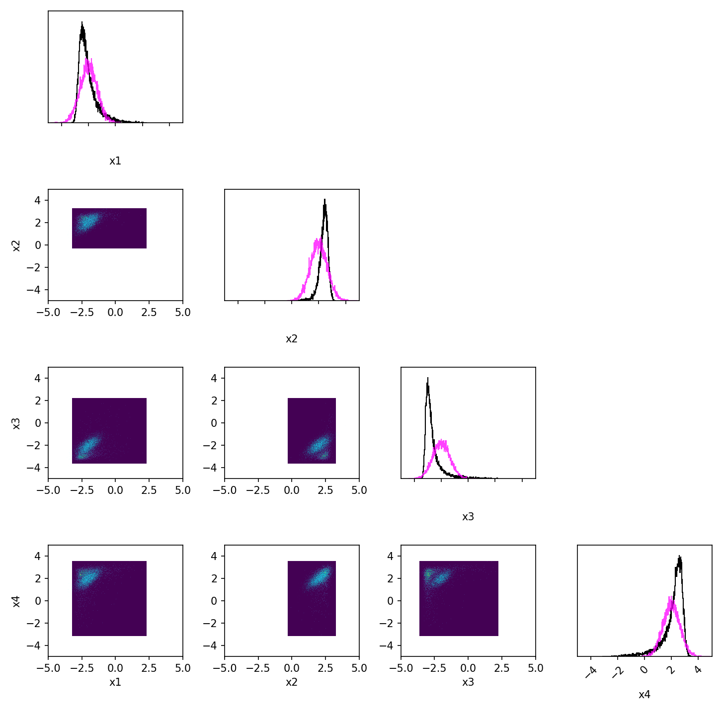
Figure F.2: Gaussian4D experiment. The target distribution is depicted by light blue contour points and its marginal by a pink curve. The learned diffusion model is depicted by greenish blue contour sample points and its marginal by a black curve.

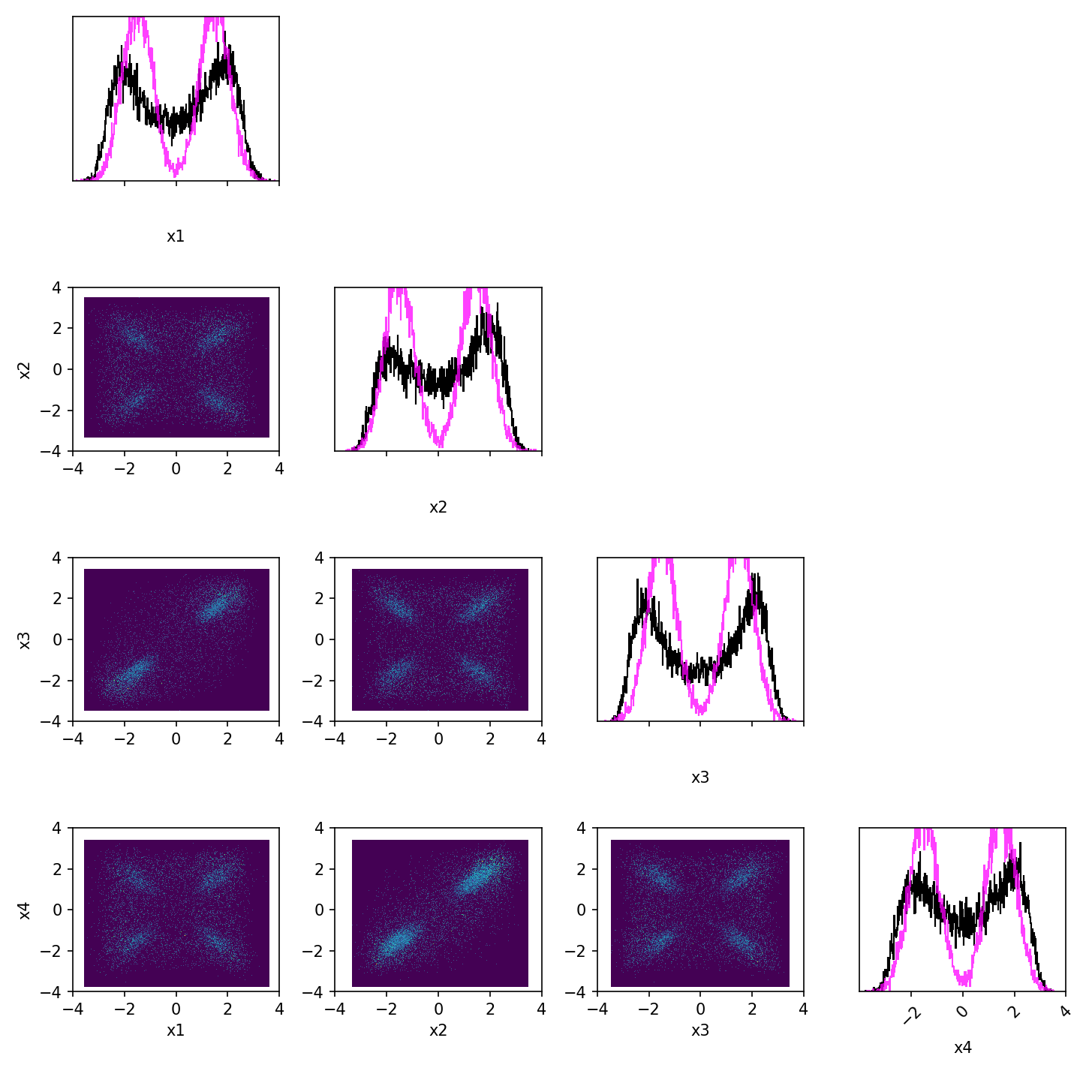
Figure F.3: Mixturegaussians4D experiment. The target distribution is depicted by light blue contour points and its marginal by a pink curve. The learned diffusion model is depicted by greenish blue contour sample points and its marginal by a black curve.

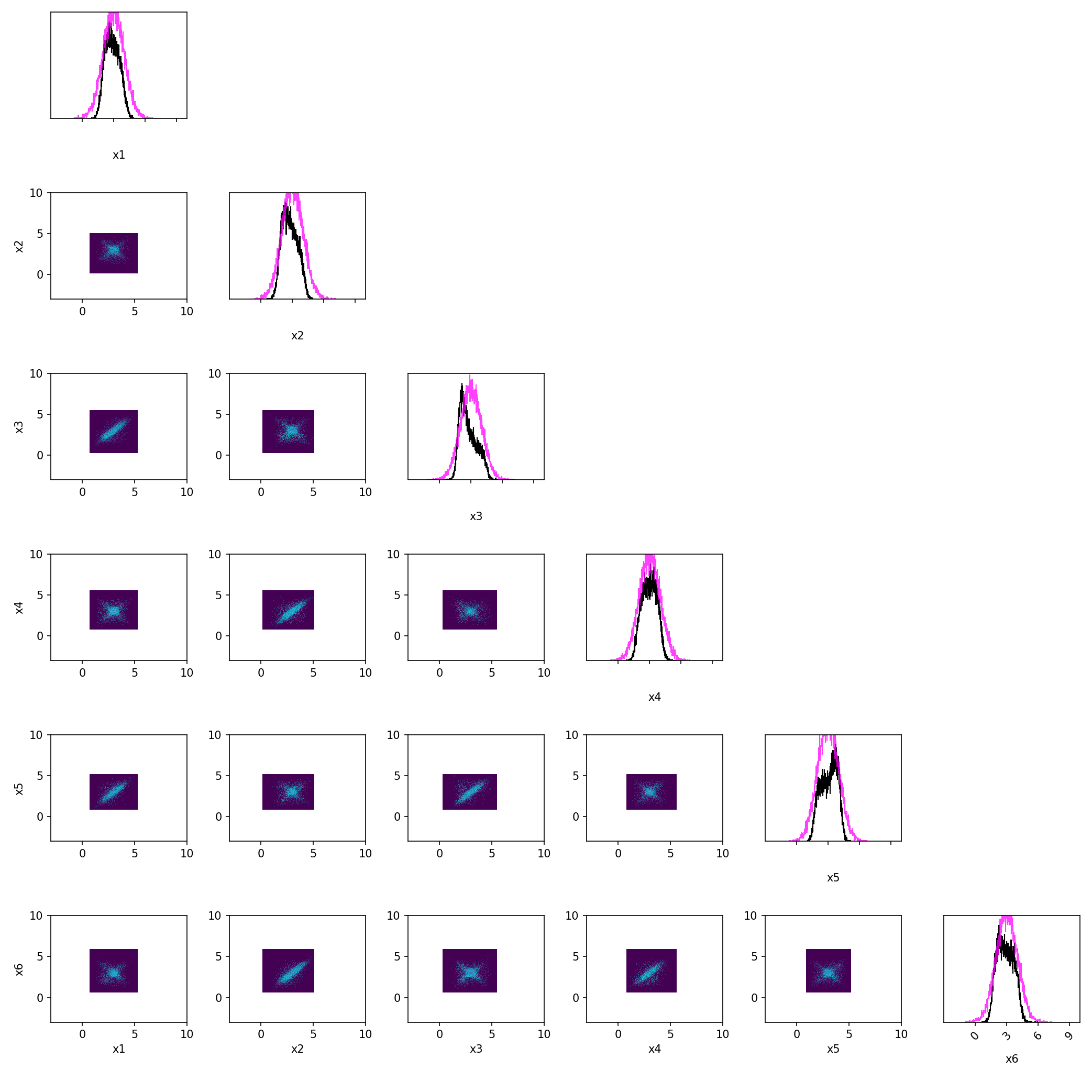
Figure F.4: Stargaussian6D experiment. The target distribution is depicted by light blue contour points and its marginal by a pink curve. The learned diffusion model is depicted by greenish blue contour sample points and its marginal by a black curve.

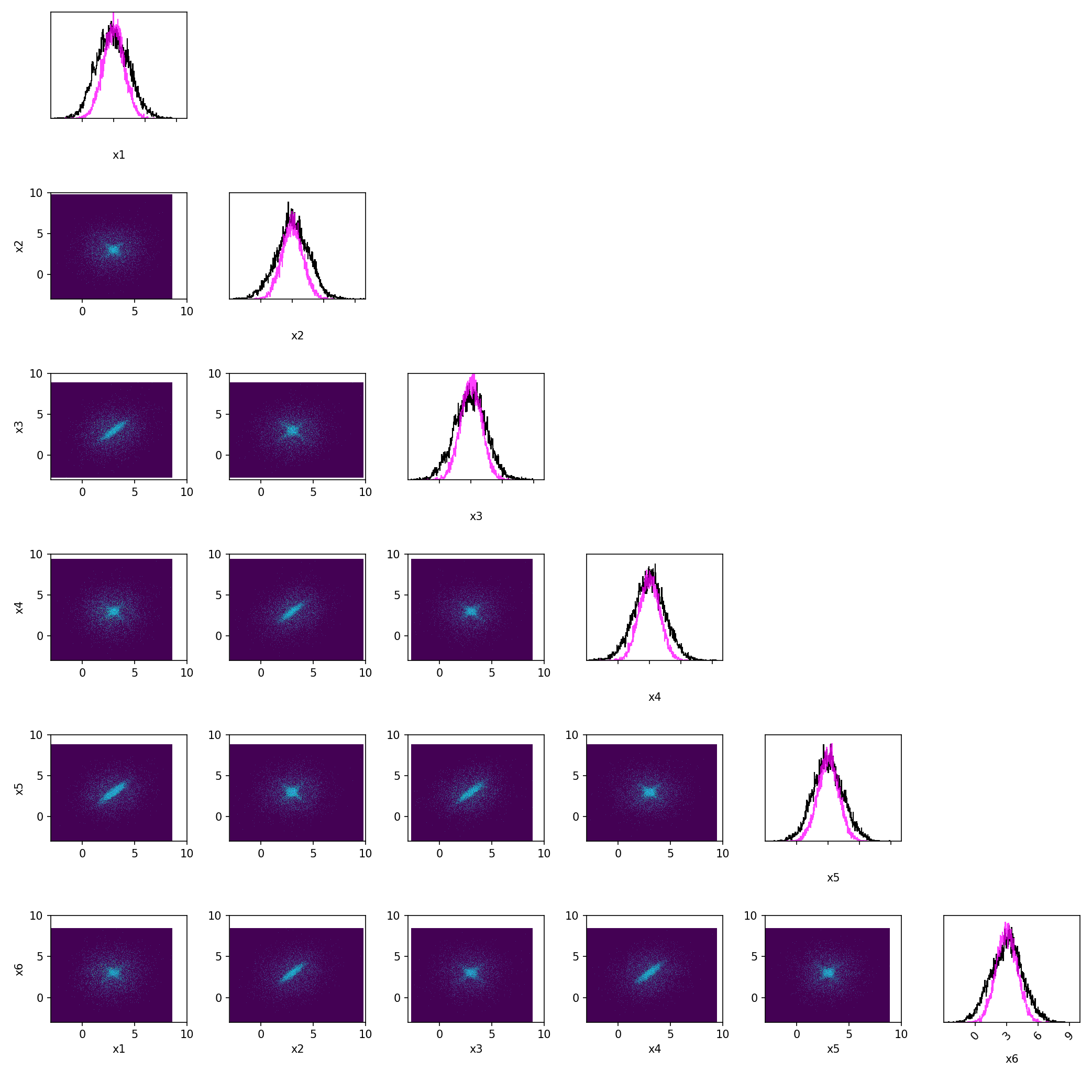
Figure F.5: Stargaussian6D experiment when using the baseline flow-based method. The target distribution is depicted by light blue contour points and its marginal by a pink curve. The learned flow model is depicted by greenish blue contour sample points and its marginal by a black curve.

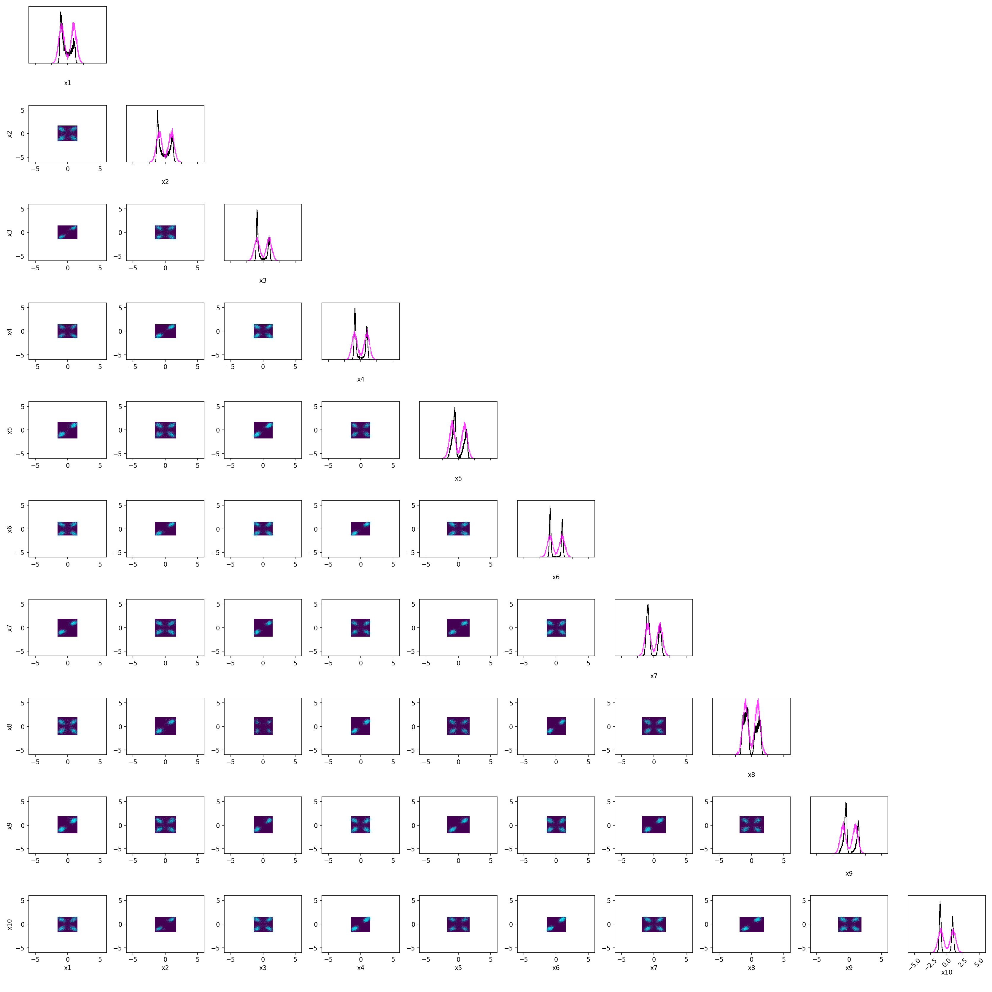
Figure F.6: Mixturegaussians10D experiment. The target distribution is depicted by light blue contour points and its marginal by a pink curve. The learned diffusion model is depicted by greenish blue contour sample points and its marginal by a black curve.

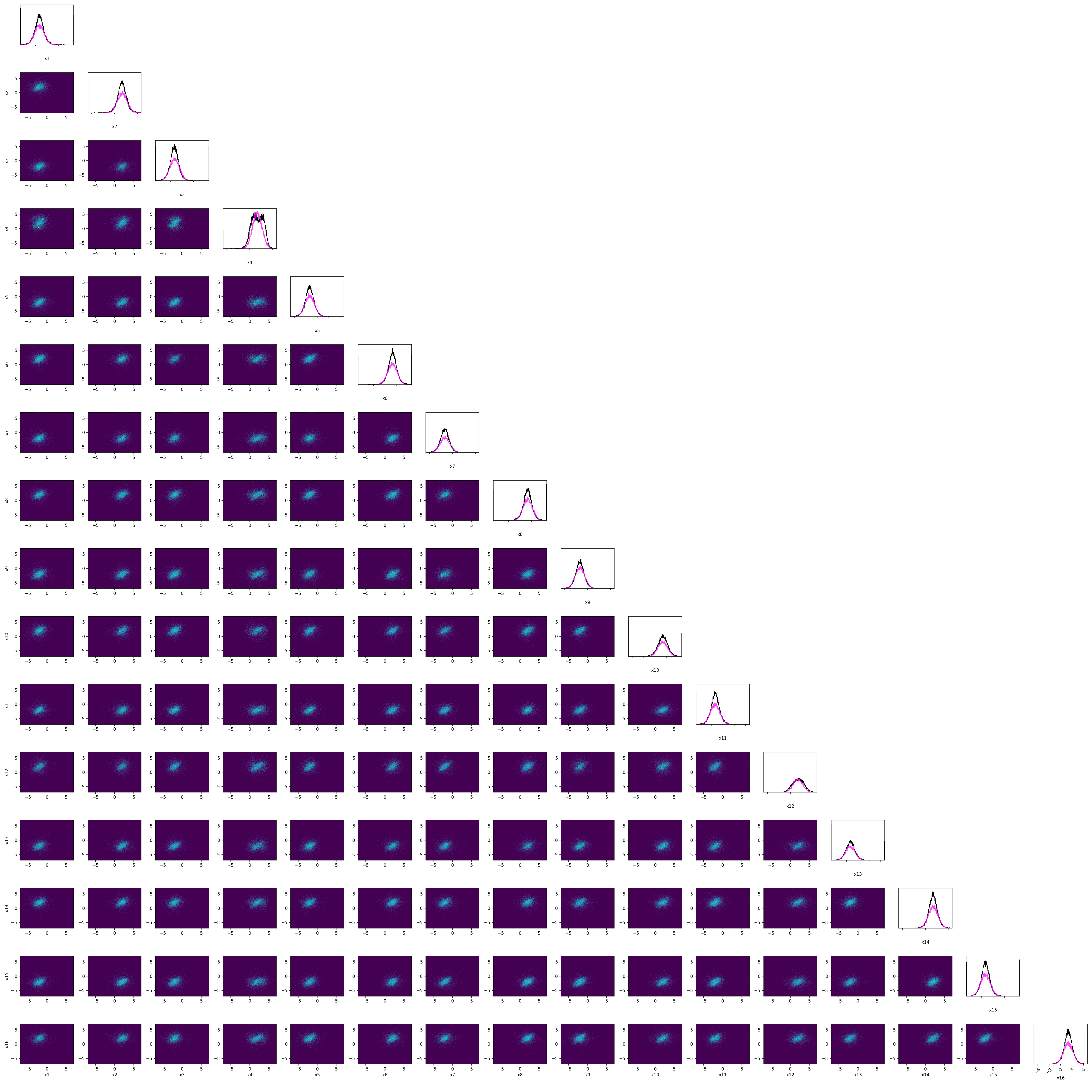
Figure F.7: Gaussian16D experiment. The target distribution is depicted by light blue contour points and its marginal by a pink curve. The learned diffusion model is depicted by greenish blue contour sample points and its marginal by a black curve.

F.2 LLM experiment

Details of the data generation for the LLM experiment, including the prompts used, are provided in Mikkola et al. (2024, Appendix C.2). We reuse their data and scripts to convert the 5-wise rankings into the pairwise comparisons assumed in our setup: https://github.com/petrus-mikkola/prefflow.

Fig. F.8 shows completes the partial plot in main text for the LLM experiment. The elicited $2d$ and $1d$ marginals have the same support as the true data distribution marginals, and their shapes are also similar, with the distinction that score-based methods tend to generate Gaussian-like marginals. The only exception is the variable AveOccup, whose marginal appears to have an unreasonably long tail.

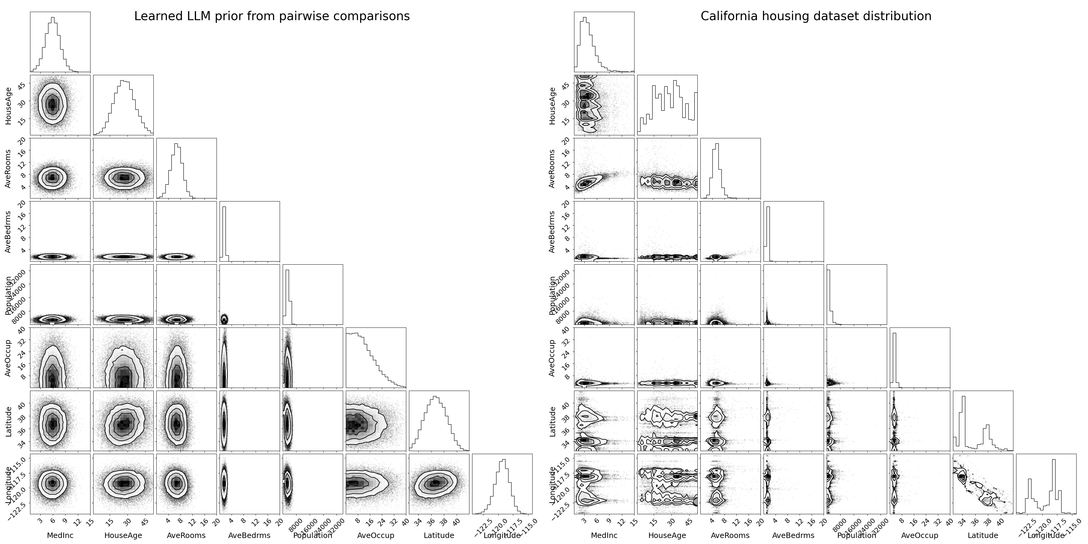
Figure F.8: Full result plot for the LLM expert elicitation experiment, complementing the partial plot presented in Fig. 7(a).

Fig. F.9 compares our score-based diffusion method and the flow method of learning the LLM prior from pairwise comparisons in the LLM experiment, highlighting that score-based method result in smoother estimates than the flow method. Table F.1 summarizes the densities in a quantitative manner by reporting the means for all variables.

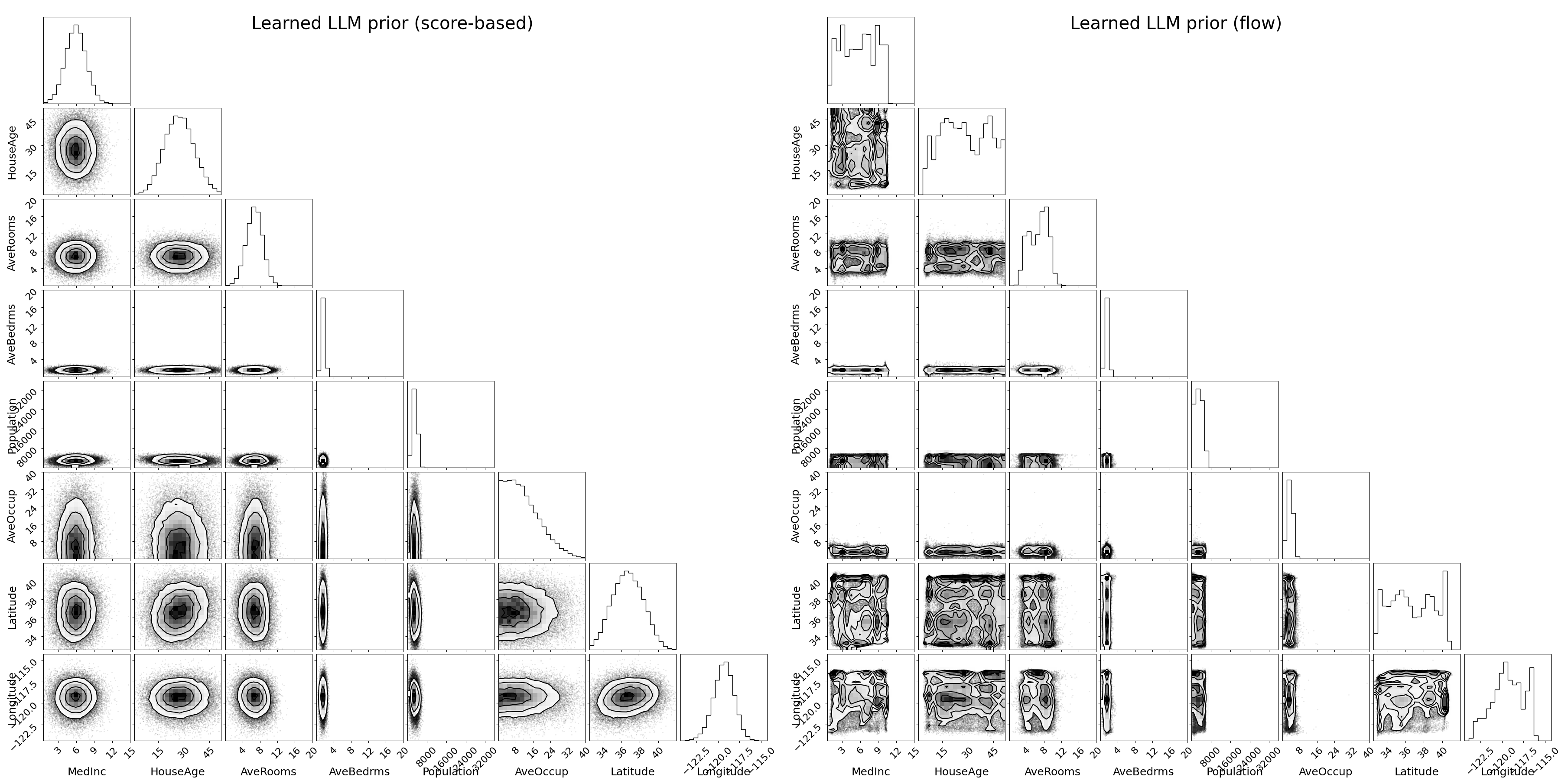
Figure F.9: Comparison of the results when learning the LLM prior from pairwise comparisons using our score-based diffusion method (left) and the flow based method (right).

Table F.1: The means of the variables based on (first row) the distribution of California housing dataset, (second row) the sample from the score-based diffusion model fitted to the LLM’s feedback, and (third row) the sample from the flow model.

	MedInc	HouseAge	AveRooms	AveBedrms	Population	AveOccup	Lat	Long
True data	3.87	28.64	5.43	1.1	1425.48	3.07	35.63	-119.57
Score-based	5.89	27.56	6.66	1.53	2997.96	4.70	36.69	-119.37
Flow	5.83	28.48	6.68	1.49	2948.17	3.36	36.73	-119.30

References

- Acerbi (2020) Luigi Acerbi. Variational Bayesian Monte Carlo with noisy likelihoods. Advances in Neural Information Processing Systems, 33:8211–8222, 2020.
- Anderson (1982) Brian Anderson. Reverse-time diffusion equation models. Stochastic Processes and their Applications, 12(3):313–326, 1982.
- Anthropic (2024) Anthropic. The Claude 3 Model Family: Opus, Sonnet, Haiku. https://www-cdn.anthropic.com/de8ba9b01c9ab7cbabf5c33b80b7bbc618857627/Model_Card_Claude_3.pdf, 2024. Model card.
- Becker et al. (1963) Gordon M Becker, Morris H DeGroot, and Jacob Marschak. Stochastic models of choice behavior. Behavioral science, 8(1):41–55, 1963.
- Bradley & Terry (1952) Ralph Allan Bradley and Milton Terry. Rank analysis of incomplete block designs: I. the method of paired comparisons. Biometrika, 39(3/4):324–345, 1952.
- Chen (2018) Ricky TQ Chen. torchdiffeq, 2018. URL https://github.com/rtqichen/torchdiffeq.
- Chen et al. (2018) Ricky TQ Chen, Yulia Rubanova, Jesse Bettencourt, and David K Duvenaud. Neural ordinary differential equations. Advances in Neural Information Processing Systems, 31, 2018.
- Chu & Ghahramani (2005) Wei Chu and Zoubin Ghahramani. Preference learning with Gaussian processes. In Proceedings of the 22nd International Conference on Machine learning, pp. 137–144, 2005.
- Dehaene (2003) Stanislas Dehaene. The neural basis of the Weber–Fechner law: a logarithmic mental number line. Trends in cognitive sciences, 7(4):145–147, 2003.
- Dumoulin et al. (2024) Vincent Dumoulin, Daniel D. Johnson, Pablo Samuel Castro, Hugo Larochelle, and Yann Dauphin. A density estimation perspective on learning from pairwise human preferences. Transactions on Machine Learning Research, 2024. ISSN 2835-8856.
- Flanders (1973) Harley Flanders. Differentiation under the integral sign. The American Mathematical Monthly, 80(6):615–627, 1973.
- Fürnkranz & Hüllermeier (2010) Johannes Fürnkranz and Eyke Hüllermeier. Preference learning and ranking by pairwise comparison. In Preference learning, pp. 65–82. Springer, 2010.
- Gloeckler et al. (2024) Manuel Gloeckler, Michael Deistler, Christian Dietrich Weilbach, Frank Wood, and Jakob H Macke. All-in-one simulation-based inference. In Proceedings of the 41th International Conference on Machine Learning, pp. 15735–15766. PMLR, 2024.
- Grathwohl et al. (2019) Will Grathwohl, Ricky TQ Chen, Jesse Bettencourt, Ilya Sutskever, and David Duvenaud. Ffjord: Free-form continuous dynamics for scalable reversible generative models. In International Conference on Learning Representations, 2019.
- Hendrycks & Gimpel (2016) Dan Hendrycks and Kevin Gimpel. Gaussian error linear units (gelus). arXiv preprint arXiv:1606.08415, 2016.
- Ho et al. (2020) Jonathan Ho, Ajay Jain, and Pieter Abbeel. Denoising diffusion probabilistic models. Advances in Neural Information Processing Systems, 33:6840–6851, 2020.
- Karras et al. (2022) Tero Karras, Miika Aittala, Timo Aila, and Samuli Laine. Elucidating the design space of diffusion-based generative models. Advances in Neural Information Processing Systems, 35:26565–26577, 2022.
- Karras et al. (2024a) Tero Karras, Miika Aittala, Tuomas Kynkäänniemi, Jaakko Lehtinen, Timo Aila, and Samuli Laine. Guiding a diffusion model with a bad version of itself. In Advances in Neural Information Processing Systems, volume 37, pp. 52996–53021, 2024a.
- Karras et al. (2024b) Tero Karras, Miika Aittala, Jaakko Lehtinen, Janne Hellsten, Timo Aila, and Samuli Laine. Analyzing and improving the training dynamics of diffusion models. In Proceedings of the IEEE/CVF Conference on Computer Vision and Pattern Recognition, pp. 24174–24184, 2024b.
- Kendall & Babington Smith (1940) M. G. Kendall and B. Babington Smith. On the method of paired comparisons. Biometrika, 31(3/4):324–345, March 1940.
- Kingma & Ba (2015) Diederik P. Kingma and Jimmy Ba. Adam: A method for stochastic optimization. In International Conference on Learning Representations, 2015.
- Leike et al. (2018) Jan Leike, David Krueger, Tom Everitt, Miljan Martic, Vishal Maini, and Shane Legg. Scalable agent alignment via reward modeling: a research direction. arXiv preprint arXiv:1811.07871, 2018.
- Li et al. (2024) Xiang Li, Yixiang Dai, and Qing Qu. Understanding generalizability of diffusion models requires rethinking the hidden Gaussian structure. Advances in Neural Information Processing Systems, 37:57499–57538, 2024.
- Lipman et al. (2023) Yaron Lipman, Ricky T. Q. Chen, Heli Ben-Hamu, Maximilian Nickel, and Matthew Le. Flow matching for generative modeling. In International Conference on Learning Representations, 2023.
- Loshchilov & Hutter (2019) Ilya Loshchilov and Frank Hutter. Decoupled weight decay regularization. In International Conference on Learning Representations, 2019.
- Mikkola et al. (2023) Petrus Mikkola, Osvaldo A. Martin, Suyog Chandramouli, Marcelo Hartmann, Oriol Abril Pla, Owen Thomas, Henri Pesonen, Jukka Corander, Aki Vehtari, Samuel Kaski, Paul-Christian Bürkner, and Arto Klami. Prior Knowledge Elicitation: The Past, Present, and Future. Bayesian Analysis, pp. 1 – 33, 2023.
- Mikkola et al. (2024) Petrus Mikkola, Luigi Acerbi, and Arto Klami. Preferential normalizing flows. In Advances in Neural Information Processing Systems, 2024.
- Nicoli et al. (2023) Kim A Nicoli, Christopher J Anders, Tobias Hartung, Karl Jansen, Pan Kessel, and Shinichi Nakajima. Detecting and mitigating mode-collapse for flow-based sampling of lattice field theories. Physical Review D, 108(11):114501, 2023.
- O’Hagan (2019) Anthony O’Hagan. Expert knowledge elicitation: Subjective but scientific. The American Statistician, 73:69–81, 2019.
- Ouyang et al. (2022) Long Ouyang, Jeffrey Wu, Xu Jiang, Diogo Almeida, Carroll Wainwright, Pamela Mishkin, Chong Zhang, Sandhini Agarwal, Katarina Slama, Alex Ray, et al. Training language models to follow instructions with human feedback. Advances in Neural Information Processing Systems, 35:27730–27744, 2022.
- Pace & Barry (1997) R Kelley Pace and Ronald Barry. Sparse spatial autoregressions. Statistics & Probability Letters, 33(3):291–297, 1997.
- Rezende & Mohamed (2015) Danilo Rezende and Shakir Mohamed. Variational inference with normalizing flows. In International Conference on Machine learning, pp. 1530–1538. PMLR, 2015.
- Rombach et al. (2022) Robin Rombach, Andreas Blattmann, Dominik Lorenz, Patrick Esser, and Björn Ommer. High-resolution image synthesis with latent diffusion models. In Proceedings of the IEEE/CVF Conference on Computer Vision and Pattern Recognition, pp. 10684–10695, June 2022.
- Rosenblatt (1952) Murray Rosenblatt. Remarks on a multivariate transformation. The annals of mathematical statistics, 23(3):470–472, 1952.
- Shah & Oppenheimer (2008) Anuj K Shah and Daniel M Oppenheimer. Heuristics made easy: an effort-reduction framework. Psychological Bulletin, 134(2):207, 2008.
- Song & Ermon (2019) Yang Song and Stefano Ermon. Generative modeling by estimating gradients of the data distribution. Advances in Neural Information Processing Systems, 2019.
- Song et al. (2021) Yang Song, Jascha Sohl-Dickstein, Diederik P Kingma, Abhishek Kumar, Stefano Ermon, and Ben Poole. Score-based generative modeling through stochastic differential equations. In International Conference on Learning Representations, 2021.
- Stimper et al. (2022) Vincent Stimper, Bernhard Schölkopf, and José Miguel Hernández-Lobato. Resampling base distributions of normalizing flows. In International Conference on Artificial Intelligence and Statistics, pp. 4915–4936. PMLR, 2022.
- Thurstone (1927) L. L. Thurstone. A law of comparative judgment. Psychological Review, 34(4):273–286, 1927.
- Touvron et al. (2023) Hugo Touvron, Louis Martin, Kevin Stone, Peter Albert, Amjad Almahairi, Yasmine Babaei, Nikolay Bashlykov, Soumya Batra, Prajjwal Bhargava, Shruti Bhosale, et al. Llama 2: Open foundation and fine-tuned chat models. arXiv preprint arXiv:2307.09288, 2023.
- Train (2009) Kenneth E Train. Discrete choice methods with simulation. Cambridge university press, 2009.
- Vincent (2011) Pascal Vincent. A connection between score matching and denoising autoencoders. Neural computation, 23(7):1661–1674, 2011.
- Wallace et al. (2024) Bram Wallace, Meihua Dang, Rafael Rafailov, Linqi Zhou, Aaron Lou, Senthil Purushwalkam, Stefano Ermon, Caiming Xiong, Shafiq Joty, and Nikhil Naik. Diffusion model alignment using direct preference optimization. In Proceedings of the IEEE/CVF Conference on Computer Vision and Pattern Recognition, pp. 8228–8238, 2024.
- Wang et al. (2023) Zhendong Wang, Yifan Jiang, Huangjie Zheng, Peihao Wang, Pengcheng He, Zhangyang Wang, Weizhu Chen, Mingyuan Zhou, et al. Patch diffusion: Faster and more data-efficient training of diffusion models. Advances in Neural Information Processing Systems, pp. 72137–72154, 2023.
- Welling & Teh (2011) Max Welling and Yee W Teh. Bayesian learning via stochastic gradient Langevin dynamics. In Proceedings of the 28th International Conference on Machine learning, pp. 681–688, 2011.