Euclid preparation

The Euclid satellite will provide data on the clustering of galaxies and on the distortion of their measured shapes, which can be used to constrain and test the cosmological model. However, the increase in precision places strong requirements on the accuracy of the theoretical modelling for the observables and of the full analysis pipeline. In this paper, we investigate the accuracy of the calculations performed by the Cosmology Likelihood for Observables in Euclid (CLOE), a software able to handle both the modelling of observables and their fit against observational data for both the photometric and spectroscopic surveys of Euclid, by comparing the output of CLOE with external codes used as benchmark. We perform such a comparison on the quantities entering the calculations of the observables, as well as on the final outputs of these calculations. Our results highlight the high accuracy of CLOE when comparing its calculation against external codes for Euclid observables on an extended range of operative cases. In particular, all the summary statistics of interest always differ less than $0.1\,\sigma$ from the chosen benchmark, and CLOE predictions are statistically compatible with simulated data obtained from benchmark codes. The same holds for the comparison of correlation function in configuration space for spectroscopic and photometric observables.

1 Introduction

The current decade will see cosmological investigations profit from a significant increase in the precision of data, particularly those related to observations of the large-scale structure (LSS). Several galaxy surveys, such as Euclid (Laureijs et al. 2011; Euclid Collaboration: Mellier et al. 2025), the Vera C. Rubin Legacy Survey of Space and Time (LSST; Ivezić et al. 2019), and the Nancy Grace Roman Space Telescope (Spergel et al. 2015), will observe the position and shape of billions of galaxies. This will allow us to obtain information on their clustering as well as on the lensing effect that intervening matter has on their shapes, thus effectively mapping the distribution of galaxies and matter across the Universe.

The main goal of such observations is to shed light on what are key open questions in the cosmological community, such as understanding the mechanism responsible for the late-time acceleration of the expansion of the Universe (Riess et al. 1998; Perlmutter et al. 1999). Current models range from those that require the presence of a scalar field induced by a dark energy component (Peebles & Ratra 2003) to others that instead invoke a modification of the laws of General Relativity on cosmological scales (Clifton et al. 2012). At the same time, other fundamental questions and goals are related to the nature of dark matter (Feng 2010), the measurement of the mass of neutrinos via their impact on the LSS (Lesgourgues & Pastor 2006), as well as a potential detection of primordial non-Gaussianities in the epoch immediately after inflation (Desjacques & Seljak 2010). All of these components leave distinctive imprints on the LSS observables, since they can strongly affect the large-scale matter and galaxy distribution expected from the standard model of cosmology, based on cold pressureless dark matter and on a cosmological constant ($\varLambda\mathrm{CDM}$).

The Euclid mission (Laureijs et al. 2011) was specifically designed to tackle these open questions, and is expected to deliver a significant improvement of our knowledge in these fields (Euclid Collaboration: Mellier et al. 2025). However, in order to achieve these goals, the exquisite precision of the measurements that will be collected by Stage-IV surveys demands a corresponding level of accuracy in the theoretical modelling of the LSS observables.

For this reason, the Euclid Collaboration has decided to dedicate a major effort to the development of a software to compute theoretical predictions for the main scientific observables: the Cosmology Likelihood for Observables in Euclid (CLOE). This code implements the modelling of the primary photometric and spectroscopic observables that will be used by Euclid, following the theoretical recipe described in Euclid Collaboration: Cardone et al. (2025), hereafter Paper 1. Building a standalone likelihood and theory code for Euclid is essential, as we aim to establish a homogeneous and flexible framework that consistently models the primary probes of the mission – weak lensing and galaxy clustering – within a unified approach. Furthermore, the decision to build a new code for the analysis of Euclid data allows us to improve the modelling and analysis of systematic effects. Indeed, CLOE includes nuisance parameters that capture effects that could be neglected in previous analyses, given the lower sensitivity with respect to Euclid. Moreover, it is fully written in Python, while still achieving the performance required by a likelihood analysis. More information on these new implementations is provided in Paper 1 and Euclid Collaboration: Joudaki et al. (2025), hereafter Paper 2.

At the practical level, CLOE obtains theoretical predictions given a set of cosmological parameters making use of an interface with Cobaya (Torrado & Lewis 2021), which can retrieve the main ingredients for our theoretical expectations from publicly available Boltzmann solvers, CAMB (Lewis et al. 2000; Howlett et al. 2012) and CLASS (Blas et al. 2011). The structure of CLOE, its interface with Cobaya, and the way theoretical calculations are performed are presented in detail in Paper 2.

In addition to the computation of cosmological observables, the interface with Cobaya allows the user to employ CLOE as a likelihood code, which means to compare the theoretical predictions with observational data. By sampling the parameter space and performing such a comparison iteratively, CLOE allows us to infer the probability distribution of the free parameters of the model under analysis. This procedure is described in Euclid Collaboration: Caas-Herrera et al. (2025), hereafter Paper 3, where CLOE is used to derive forecasts on the parameters of the $\varLambda\mathrm{CDM}$ model and some of its extensions (e.g. $w_{0}w_{\rm a}$CDM, non-flat cosmologies) from synthetic Euclid data using a realistic set of Monte Carlo Markov chain (MCMC) runs.

The increased precision of observations that we expect from Euclid requires the inclusion of several systematic effects in the modelling of the observables, as neglecting these can yield significant biases on the final results obtained while analysing the data (Tutusaus et al. 2020; Martinelli et al. 2021). Given the complexity of some of the calculations required, it is crucial to assess the accuracy of CLOE, in order to ensure the quality of the computed theoretical predictions. The choices made in performing the calculations, such as the numerical integrations or the sampling of cosmological functions in redshift and scale, can significantly affect the output of the code and, consequently, the results of the analysis. For this reason, in this paper, we aim to compare the calculations performed by CLOE against independent benchmarks, assessing the reliability of this software. This effort is similar to the benchmarking approach taken by other collaborations for codes with similar purposes, such as the Core Cosmology Library (CCL , Chisari et al. 2019) developed for LSST (LSST Science Collaboration: Abell et al. 2009; The LSST Dark Energy Science Collaboration: Mandelbaum et al. 2018). While in this paper our aim is to validate the accuracy of our calculations, the impact of the systematic effects modelled within CLOE will instead be investigated in a subsequent publication (Euclid Collaboration: Blot et al. 2025).

To reach our goal, we assess the accuracy of the theoretical calculations performed by CLOE, benchmarking them against the results of external codes. We quantify the agreement in units of the observational error, thus ensuring that any difference found is much lower than the statistical uncertainty and, therefore, that it will not impact the real-data analysis. While in this work we provide an assessment of the accuracy of CLOE calculations, an extensive investigation of the methodology used to obtain the observables, their uncertainty, together with a comparison between different nonlinear recipes, will be presented in Euclid Collaboration: Crocce et al. (2025), Euclid Collaboration: Carrilho et al. (2025), Euclid Collaboration: Moretti et al. (2025) and Euclid Collaboration: Sciotti et al. (2025).

This paper is structured as follows. In Sect. 2 we describe the external codes used to obtain the benchmarks on the observables of interest, while in Sect. 3 we provide details on the settings used for the validation, describing the different effects taken into account, as well as the cosmological assumptions. In Sect. 4, we outline the methods used to validate CLOE against independent codes, and we define the metrics used to assess their agreement. Section 5 contains the validation results for the observables related to the spectroscopic and photometric observables surveys, including the intermediate quantities that are used to perform these calculations. We draw our conclusions in Sect. 7.

2 External codes and setup for benchmark generation

Table 1: Summary of the connections between the equations in Paper 1 and the CLOE quantities discussed in this work.

Quantity	Expression	Equation
Weak lensing power spectrum	$C_{ij}^{\rm LL}(\ell)$	(32)
Photometric galaxy power spectrum	$C_{ij}^{\rm GG}(\ell)$	(40)
Galaxy-galaxy lensing power spectrum	$C_{ij}^{\rm GL}(\ell)$	(54)
Weak lensing correlation function	$\xi_{ij}^{\pm}(\theta)$	(70)
Photometric galaxy correlation function	$\xi_{ij}^{\rm GG}(\theta)$	(73)
Galaxy-galaxy lensing correlation function	$\xi_{ij}^{\rm GL}(\theta)$	(74)
Power spectrum Legendre multipoles	$P_{\ell}(k,z)$	(90)
AP-distorted power spectrum Legendre multipoles	$P_{\rm obs,\ell}(k^{\rm fid},z)$	(94)
Correlation function Legendre multipoles	$\xi_{{\rm obs},\ell}(s^{\rm fid},z)$	(104)

As the purpose of this paper is to validate the predictions obtained with CLOE, we compare its results with those from external codes that have been previously validated, at least in a subset of the relevant cases. This section provides a description of these external codes, along with their corresponding references, and outlines the setup adopted to generate the benchmark predictions used for comparison throughout the paper.

In this work, we do not define all the observables that will be compared with external codes. The definition of these can be found in Paper 1, where the intermediate quantities used for the calculations are also defined. We report in Table 1 the reference for the equations of the observables we will discuss, in order to facilitate their retrieval in Paper 1.

2.1 External benchmark for 3$\times$2pt

The main observable of the photometric survey of Euclid is the set of angular power spectra $C^{AB}_{ij}(\ell)$, defined in Paper 1, for weak lensing, galaxy clustering and their cross-correlation. These spectra are obtained from CLOE for all the redshift bin combinations given a binned galaxy distribution. We compute the $C^{AB}_{ij}(\ell)$ in 270 multipole bins, logarithmically spaced. Similarly, we consider the projection of the power spectra into the two-point correlation function (2PCF) $\xi^{\rm GG}_{ij}(\theta)$, $\xi^{-}_{ij}(\theta)$, $\xi^{+}_{ij}(\theta)$, and $\xi^{\rm GL}_{ij}(\theta)$, also defined in Paper 1. These correlation functions are computed in 40 logarithmically spaced bins in the angle $\theta$, contained in the interval $\theta\in\left[0.1,10\right]\,\deg$.

For what concerns the predictions of CLOE for photometric observables, we rely on two different codes to produce benchmarks: LiFE and CCL. While CCL is a code that has already been extensively used by the cosmological community, this is not the case for LiFE, which is a private code developed to obtain predictions for the Euclid survey.

However, due to differences in the assumed recipe, we cannot compare CLOE with CCL for all the cases detailed in Sect. 3. Therefore, we choose to present most of our validation results focusing on LiFE, while we show the outcome of the comparison with CCL, for the cases where this is possible, in Appendix B.

2.1.1 LiFE

LiFE (Likelihood and Forecasts for Euclid) is a collection of codes written in Mathematica to perform the computation of the 3×2pt observables for likelihood evaluation and Fisher matrix forecasts. It has been validated against the code implementation adopted during the Fisher forecast analysis from Euclid Collaboration: Blanchard et al. (2020), checking that, for the same settings, it provides the same estimates of the marginalised constraints on the cosmological parameters, also comparing the intermediate quantities used in calculations. Although not optimised and much slower than any Python implementation, LiFE has been designed with the validation of CLOE in mind. As a consequence, the same exact recipe is implemented with the possibility to turn on and off different contributions to compare against other codes too. For this same reason, it does not compute internally the matter power spectrum, but it imports it as an external quantity (to be interpolated) so that one can be sure that any difference with CLOE is not due to errors in this critical quantity. On the other hand, the fact that it is coded in a completely different language (with its own interpolation and integration routines) represents a further benefit allowing us to verify that, for the same input and the same recipe, two independent implementations yield compatible quantities, which is what we want to verify in this work.

LiFE can also be used to perform Fisher matrix forecasts for Euclid using the same assumptions (in terms of cosmological model), and settings (e.g., redshift distributions, number of redshift bins and angular multipoles) adopting a semi-analytic method to compute the derivatives of the observables. Although it is well known that the Fisher matrix method provides lower limits on the marginalised constraints on the cosmological parameters under the assumption of Gaussian likelihood, these forecasts can be used to check that the results from MCMC inference are in the same ballpark (see Paper 3, ).

2.1.2 CCL

CCL is a modern cosmological library designed to compute a large number of cosmological observables for a variety of cosmological models. These range from background quantities, power spectra and correlation functions to halo model ingredients; it is interfaced with both CAMB – the default choice – and CLASS, and it has been extensively validated against existing codes (Chisari et al. 2019). The core of CCL is developed in C, allowing it to achieve high performance. However, a thoroughly documented Python interface, PyCCL, is also available, combining in this way efficiency and user-friendliness.

For the present exercise, we use the third release of the code (more specifically, v3.0.2). The theory predictions are computed using as inputs the cosmological parameters, redshift distributions, and systematics defined in Sect. 3.1, as well as the matter power spectrum extracted from CLOE; the growth factor is instead obtained from CCL itself. The harmonic-space power spectra are computed in the Limber approximation via the QAG adaptive integration method of GSL (GNU Scientific Library, Galassi et al. 2009); these are then transformed into the 2PCF via the FFTlog method.
The CCL routines can produce all the cases listed in Table 2, except for the ones including Redshift space distortions (RSD) (i.e., P23 and from P11 to P22), for which the recipe implemented differs from the one used in CLOE, which, as outlined in Paper 1, follows Tanidis & Camera (2019). For these cases, only the comparison with LiFE will be shown. The results of the comparison against CCL can be found in Appendix B.

2.2 External benchmark for GCsp

The main observable of the spectroscopic survey of Euclid is the set of Legendre multipoles of the anisotropic galaxy power spectrum, $P_{\mathrm{obs},\ell}(k^{\mathrm{fid}},z)$, as defined in Paper 1 and Euclid Collaboration: Moretti et al. (2025). These multipoles are obtained by projecting the two-dimensional anisotropic power spectrum onto the Legendre polynomials $\mathcal{L}_{\ell}(\mu)$. Under the assumptions of linear theory, only the first three even multipoles are non-vanishing, corresponding to $\ell\in{0,2,4}$. Similarly, in configuration space, we consider an equivalent expansion over the Legendre polynomials, leading to the 2PCF Legendre multipoles, $\xi_{{\rm obs},\ell}(s^{\rm fid},z)$.

For the purpose of the validation carried out here, we generate external benchmark predictions without including geometrical distortions caused by adopting a fiducial cosmology that differs from the true one. In other words, we neglect the AlcockPaczynski (AP; Alcock & Paczynski 1979) effect, which would rescale the transverse ($k_{\perp}$) and line-of-sight ($k_{\parallel}$) components of the wavevector $k$. As a result, the effective quantities we compare are the Legendre multipoles of the power spectrum, $P_{\ell}(k,z)$, computed without AP corrections. Since AP effects depend solely on background quantities, which are validated separately in Appendix C, we do not explore their impact further in this work.

In all cases defined in Sect. 3.2 for the power spectrum Legendre multipoles, the data vectors and covariance matrices are computed at the mean redshift of four distinct redshift bins, namely $\{(0.9,1.1),\ (1.1,1.3),\ (1.3,1.5),\ (1.5,1.8)\}$, and are sampled using 350 linear $k$ bins over the range $(0.001,\,0.35)\,\mathrm{Mpc}^{-1}$. On the contrary, for the validation carried out in configuration space, the 2PCF is sampled with linear bins of $\varDelta s=5\,{\rm Mpc}$ over the range $(37.5,387.5)\,{\rm Mpc}$.

The external benchmarks are produced using two different codes, PBJ and COFFE. While the former adopts the same nonlinear modelling recipe as CLOE in Fourier space, the latter offers a convenient framework to test the pipeline that converts Legendre multipoles from Fourier to configuration space. In the following sections, we briefly summarise the main features of the two codes.

2.2.1 PBJ

The implementation of the nonlinear model in CLOE is validated against that in the Power spectrum Bispectrum Joint code (PBJ), a non-public Python package that has been employed in several analyses involving the full shape of the galaxy power spectrum, $P_{\rm gg}(\bm{k})$, and bispectrum, $B_{\rm ggg}(\bm{k}_{1},\bm{k}_{2})$. These include both comparisons to numerical simulations in the context of model selection (Oddo et al. 2020, 2021), as well as cosmological inference from real data, such as the recent analysis of the BOSS DR12 sample (Moretti et al. 2023).

The code features an implementation of the widely adopted effective field theory of large-scale structure (EFTofLSS) model, based on the same theoretical prescription presented in Euclid Collaboration: Pezzotta et al. (2024), which is precisely what has been reproduced in the current version of CLOE. A common feature of models based on nonlinear perturbation theory and the EFTofLSS framework is that nonlinear corrections to the galaxy (and matter) power spectrum arise from the coupling of different physical scales. This coupling is mediated by kernel functions that encapsulate the physics of gravitational instability, galaxy bias, and redshift-space distortions. Specifically, the nonlinear correction $\varDelta P$ at a given wavenumber $k$ can be expressed as a convolution of the power spectrum with itself,

$$\varDelta P(k)=\int\frac{{\rm d}^{3}q}{\left(2\pi\right)^{3}}\,K(\bm{q},\bm{k}-\bm{q})\,P(\bm{q})\,P(\left|\bm{k}-\bm{q}\right|)\,,$$ (1)

where the kernel $K(\bm{q}_{1},\bm{q}_{2})$ captures the nonlinear mode coupling between the wavemodes $\bm{q}_{1}$ and $\bm{q}_{2}$. To evaluate these integrals efficiently, PBJ relies on the FASTPT library (McEwen et al. 2016), which takes advantage of the possibility to expand $K(\bm{q}_{1},\bm{q}_{2})$ in spherical harmonics, thereby enabling the use of fast Fourier transform techniques for rapid and accurate computation.

The implementation of the spectroscopic observables in CLOE follows the same approach as PBJ, and both codes adopt an identical parametrisation for the EFTofLSS nuisance parameters. This consistency allows for a direct, one-to-one comparison of each validation case described in Sect. 3.2, without the need to translate between parameter bases. As a result, we can robustly validate the CLOE predictions for the galaxy power spectrum multipoles $P_{\ell}(k)$ across all 20 benchmark scenarios presented in Sect. 3.2.

2.2.2 COFFE

The validation of the 2PCF Legendre multipoles is performed using predictions from the COrrelation Function Full-sky Estimator (COFFE) code, a public package designed to efficiently compute two-point statistics in configuration space under linear theory assumptions. In addition to the standard RSD signal, COFFE offers a rigorous treatment of several relativistic effects, including wide-angle corrections and magnification bias. We refer the reader to the COFFE-related literature for further details: theoretical modelling of relativistic effects in the 2PCF is presented in Tansella et al. (2018a), their implementation in Tansella et al. (2018b), and an assessment of the flat-sky approximation in Jelic-Cizmek (2021).

In this work, we employ COFFE to validate the accuracy of the Fourier-to-configuration space mapping used in CLOE, which is based on the numerical evaluation of a Hankel transform. For this purpose, we consider a single benchmark case based on a $\varLambda\mathrm{CDM}$ cosmology with linear-theory predictions, incorporating linear bias and the leading-order RSD effect describing large-scale infall due to galaxy peculiar velocities (Kaiser 1987).

3 Validation settings

One of the main purposes of this validation is to assess the reliability of CLOE when different effects are included in the modelling of Euclid observables. For this reason, we compare the predictions of CLOE against other benchmark codes exploring several combinations of the options available in CLOE. While we do not perform a full exploration of the parameter space, such as would be possible with a Monte Carlo approach, the selected cases are sufficient to validate the main features and systematic effects included in CLOE.

All the results presented in this paper were obtained using version v2.0.2 of CLOE, the same version used to derive forecasts in Paper 3. The theoretical framework and implementation details of this version are described in Paper 1 and Paper 2, respectively.

3.1 Photometric settings

For the validation of the photometric observables, we report 23 cases in Table 2 (labelled P01, P02, …, P23) for which we run our validation pipeline. Switching between these cases, we vary some of the settings available in CLOE to compute the observables. In particular, we focus on variations related to the following quantities.

• Cosmology: we choose $10$ different cosmologies, described in Table 3, where we report the current ($z=0$) values of the energy density parameters for matter ($\varOmega_{\rm m}$), dark energy ($\varOmega_{\rm DE}$), and baryons ($\varOmega_{\rm b}$), together with the reduced Hubble parameter ($h$), the tilt of the primordial power spectrum ($n_{\rm s}$), and the perturbation amplitude parameter $\sigma_{8}$. We include $\varLambda\mathrm{CDM}$ extensions such as evolving dark energy equation of state – described by the $w_{0}$ and $w_{a}$ parameters – and non-flat cosmologies – describing scenarios with $\varOmega_{\rm m}+\varOmega_{\rm DE}\neq 1$.

• Galaxy distribution $n(z)$: we choose different galaxy redshift distributions, matching the one used in Euclid Collaboration: Blanchard et al. (2020), labelled ISTF, the one described in Sect. 5.1 of Paper 1, labelled SPV3, and an intermediate one (SPV2), which still contains 13 bins as in SPV3, but with more irregular bin distributions.

• Intrinsic alignment (IA): we choose four cases for this systematic effect, regulated by the three IA parameters ($A_{\rm IA},\eta_{\rm IA},\beta_{\rm IA}$). These are cNLA ($0.37,0.00,0.00$), zNLA ($0.16,1.66,0.00$), eNLA ($1.720,-0.41,2.17$) and a simple noIA case ($0,0,0$) in which IA is completely neglected (see Paper 1, and references therein).

• Galaxy bias $b_{\rm g}(z)$: we consider both a binned approach, with one parameter per redshift bin, and a third-order polynomial expression to describe the $b_{\rm g}(z)$ function. For the former case, we consider an ‘unbiased’ case, with all parameters vanishing, a ‘linint’ case, where $b_{\rm g}(z)$ is obtained as the linear interpolation of the binned parameters, and a ‘constant’ case, where the bias is assumed to be constant in each redshift bin.

• Magnification bias: as for the galaxy bias, we test our calculation modelling the magnification bias using the same approaches as for $b_{\rm g}(z)$.

• RSD: we compare CLOE calculations with the external benchmark in the two available settings for the large-scale RSD effect, that is, when this is considered and when it is neglected.

Further details on the modelling of the nuisance parameters can be found in Paper 1, while their impact on the cosmological constraints will be discussed in Euclid Collaboration: Blot et al. (2025) also through a more thorough exploration of their parameter space.

Out of the cases listed in Table 2, our reference case is P23, which is also based on the settings used to generate the synthetic data for obtaining forecast results (Paper 3). While for all cases we show the summary validation values for all quantities (see Sect. 4), we will highlight in Appendix A more details for our reference, also showing the trends of the differences for each of the validated quantities.

Table 2: Validation cases in which the CLOE calculation of Euclid photometric observables are compared with external software.

Id	Cosmology	$n(z)$	IA	galaxy bias	magnification bias	RSD
P01	F1	ISTF	noIA	linint	unbiased	no
P02	F1	ISTF	cNLA	linint	unbiased	no
P03	F1	ISTF	zNLA	linint	unbiased	no
P04	F1	ISTF	eNLA	linint	unbiased	no
P05	F1	ISTF	eNLA	unbiased	unbiased	no
P06	F1	ISTF	eNLA	constant	unbiased	no
P07	F1	SPV2	eNLA	constant	unbiased	no
P08	F1	SPV3	eNLA	constant	unbiased	no
P09	F1	SPV3	eNLA	constant	linint	no
P10	F1	SPV3	eNLA	constant	constant	no
P11	F1	SPV3	eNLA	constant	unbiased	yes
P12	F1	SPV3	eNLA	constant	linint	yes
P13	F1	SPV3	eNLA	constant	constant	yes
P14	F2	SPV3	eNLA	constant	constant	yes
P15	F3	SPV3	eNLA	constant	constant	yes
P16	F4	SPV3	eNLA	constant	constant	yes
P17	F5	SPV3	eNLA	constant	constant	yes
P18	F6	SPV3	eNLA	constant	constant	yes
P19	F7	SPV3	eNLA	constant	constant	yes
P20	F8	SPV3	eNLA	constant	constant	yes
P21	F9	SPV3	eNLA	constant	constant	yes
P22	F10	SPV3	eNLA	constant	constant	yes
P23	F1	SPV3	zNLA	polynomial	polynomial	yes

Table 3: Values of the cosmological parameters in the $10$ cosmologies considered for the validation of the cosmological quantities and the main photometric and spectroscopic observables.

Id	$\varOmega_{\rm m}$	$\varOmega_{\rm DE}$	$\varOmega_{\rm b}$	$w_{0}$	$w_{a}$	$h$	$n_{\rm s}$	$\sigma_{8}$
F1	0.320	0.680	0.050	$-1.000$	0.000	0.6737	0.9660	0.8155
F2	0.317	0.676	0.051	$-1.017$	0.010	0.6775	0.9653	0.8222
F3	0.327	0.670	0.048	$-0.913$	$-0.420$	0.6704	0.9561	0.8095
F4	0.316	0.689	0.046	$-1.066$	0.313	0.6616	0.9524	0.8199
F5	0.321	0.724	0.051	$-0.914$	$-0.050$	0.6729	0.9643	0.7996
F6	0.306	0.702	0.047	$-1.039$	0.046	0.6730	0.9699	0.8248
F7	0.326	0.721	0.050	$-0.985$	0.428	0.6554	0.9461	0.8059
F8	0.307	0.664	0.045	$-1.116$	0.268	0.6724	0.9708	0.8273
F9	0.337	0.660	0.053	$-0.873$	$-0.399$	0.6658	0.9383	0.8099
F10	0.334	0.630	0.057	$-0.903$	$-0.587$	0.6720	0.9779	0.8057

3.2 Spectroscopic settings

In terms of the spectroscopic probe, we identified 20 different cases for the validation, labelled as S01, S02, …, S20. The first 10 cases assume a fixed cosmology (F1 in Table 3) and vary the nuisance parameters, whereas the last 10 cases keep the latter fixed and explore the 10 different cosmologies shown in Table 3. In terms of nuisance parameters of the EFTofLSS, we assume a minimal configuration corresponding to the one adopted to obtain MCMC forecasts in Paper 3. This includes six non-zero nuisance parameters, corresponding to the linear $b_{1}$ and quadratic bias $b_{2}$, three EFTofLSS counterterms $(c_{0},\,c_{2},\,c_{4})$ mostly meant to describe the small-scale RSD damping induced by the Fingers of God, and a shot-noise parameter $\alpha_{P}$ that models constant offsets from Poisson predictions, that is $1/\overline{n}$ (Ivanov et al. 2020; Euclid Collaboration: Crocce et al. 2025; Euclid Collaboration: Moretti et al. 2025).

On the other hand, the validation of the 2PCF is carried out assuming a single configuration based on linear theory, as described in Sect. 2.2.2. In this case we assume a $\varLambda\mathrm{CDM}$ cosmology for the comparison. Specifically, the fiducial parameters are $\varOmega_{\rm m}=0.319$, $\varOmega_{\rm DE}=0.681$, $\varOmega_{\rm b}=0.049$, $h=0.67$, $n_{\rm s}=0.96$, and $\sigma_{8}=0.83$.

4 Validation methods

The main purpose of this paper is to validate the theoretical predictions for Euclid observables obtained by CLOE against external benchmarks. While we are mostly interested in validating the final results, we also examine the intermediate quantities, which are the building blocks of the observables calculation. In this section, we present the different methods used to estimate the agreement between the quantities predicted by CLOE and the corresponding ones from the codes we use as a benchmark.

4.1 Symmetric mean absolute percentage error

When assessing the accuracy in our calculations for quantities that are not observables, thus lacking an observational error, we estimate their agreement with the benchmark using the symmetric mean absolute percentage error (SMAPE)

$${\rm SMAPE}=\frac{100}{N}\sum_{i=1}^{N}{\frac{\left|F^{\rm\texttt{CLOE}}_{i}-F^{\rm Bench}_{i}\right|}{\left(\left|F^{\rm\texttt{CLOE}}_{i}\right|+\left|F^{\rm Bench}_{i}\right|\right)/2}}\,,$$ (2)

where $F^{\rm\texttt{CLOE}}_{i}$ are the quantities computed by CLOE, $F^{\rm Bench}_{i}$ is the corresponding benchmark quantity, and the index $i$ runs over the $N$ available elements of the (vectorised) arrays.

The SMAPE estimator has the advantage of quantifying the agreement between two functions relative to the average between the compared quantities, thus without assuming which of the two is correct. Moreover, the SMAPE also allows us to obtain a single value for each of the cases in which we perform our validation (see Sect. 3), thus returning a unique estimation of agreement for each case.

The disadvantage of using this approach is that it does not allow us to observe trends in relation to redshift or scale differences. To address this issue, we also compute the value of the SMAPE at each point of the data vectors and plot it as a function of redshift or scale, depending on the quantity of interest.

4.2 Comparison of observable quantities

While we rely on the SMAPE to assess the difference against benchmark calculations for most quantities, this is not the case for the final observables. For these, we can estimate the observational uncertainty with which Euclid can obtain measurements. We choose to estimate our accuracy in terms of this uncertainty.

We define a notion of distance for a given observable $O$ as

$$d_{i}=\frac{\left|O^{\,\rm\texttt{CLOE}}_{i}-O^{\,\rm Bench}_{i}\right|}{\sigma_{O_{i}}}\,,$$ (3)

where the index $i$ runs over all the available elements of the observable array, and $\sigma_{O_{i}}$ is the observational error associated with each element, obtained using $O^{\,\rm Bench}_{i}$ as a reference to compute the error.

The distance defined in Eq. 3 allows us to visualise the difference trend by computing it for each element of the observable array. However, we also want to obtain a single value to quantify the agreement with the benchmark for each validation case. Therefore, we also compute an average and a maximum distance over each observable array, defined as

$$d_{\rm mean} =\frac{1}{N}\sum_{i=1}^{N}{d_{i}}\,,$$ (4)

$$d_{\rm max} =\max_{i}d_{i}\,.$$ (5)

With these definitions, it is possible to quantify the agreement between the observables computed by CLOE and the benchmark in terms of the Euclid precision. This allows us to define an accuracy threshold above which a difference between our calculation and the benchmark would be too significant to neglect. We set such a threshold to be $d_{\rm max}<0.1$, defining all those quantities for which the distance is within $10\%$ of the observational uncertainty as validated (Massey et al. 2012; Martinelli et al. 2021).

While the distance defined in Eq. 3 provides an intuitive quantification of the agreement between CLOE and the benchmark codes, it does not necessarily guarantee that the final results would be unbiased given any possible residual difference. Therefore, we include an additional quantification of the agreement between the codes in terms of the $\chi^{2}$. For each of the cases described in Sect. 3, we assume the observables produced by the benchmark code to be the ground truth, obtaining noisy realizations of the theory vector computed by the benchmark. This is done to place ourselves as close as possible to a typical analysis of observational data, and it allows us to test whether or not the residual differences found with the previous method are significant enough to produce biases in the data analysis.

In order to assess if the observables computed by CLOE are in agreement with the benchmark within Euclid specifications, we compute the reduced $\chi^{2}$, that is the $\chi^{2}$ divided by the number of degrees of freedom $N_{\rm dof}$, obtained by fitting CLOE predictions to the data vector generated from the benchmark quantities

$$\chi^{2}=\left(\bm{D}-\bm{T}\right)^{\rm T}\,\mathsf{K}^{-1}\,\left(\bm{D}-\bm{T}\right)\,,$$ (6)

where $\bm{D}$ and $\bm{T}$ are, respectively, the data and theory vectors, while $\mathsf{K}$ is the covariance matrix constructed following Euclid DR3 specifications.

We then assess if what we obtain falls within the limiting $\chi^{2}$ values corresponding to a given probability for our hypothesis to be true, which we choose to be $68\%$. In practice, we are assessing if the predictions of CLOE are compatible within $1\,\sigma$ with the data generated starting from the benchmark spectra. More in detail, we follow the procedure described below.

Photometric survey.

Denoting the benchmark spectra as $B_{ij}^{AB}(\ell)$, we compute the observational noise expected for Euclid DR3 as (Paper 3)

$$N_{ij}^{\rm GG}(\ell) =\frac{1}{\bar{n}_{i}}\delta_{ij}^{\rm K}\,,$$ (7)

$$N_{ij}^{\rm LL}(\ell) =\frac{\sigma_{\epsilon}^{2}}{2\,\bar{n}_{i}}\delta_{ij}^{\rm K}\,,$$ (8)

where $\bar{n}_{i}$ is the number of observed sources in the $i$-th redshift bin and $\sigma_{\epsilon}$ is the intrinsic ellipticity dispersion.

Following the approach of Sciotti et al. (2024), we use $B_{ij}^{AB}(\ell)$ and $N_{ij}^{AB}(\ell)$ to compute the covariance matrix for each of the cases under examination. The diagonal of the covariance is used to obtain the errors $\sigma_{O_{i}}$ used in Eq. 3.

In this work, we use only a Gaussian covariance, neglecting the super-sample and connected non-Gaussian terms, as well as the mode coupling introduced by the mask. For such a reason, we are effectively neglecting correlations across different multipoles, obtaining $N_{\ell}$ matrices $\mathsf{C}(\ell)$, independent from each other.

For each multipole, we construct a data vector $D_{ij}^{AB}(\ell)$ extracting a random sample from a multivariate normal with mean $B_{ij}^{AB}(\ell)$ and covariance $\mathsf{C}(\ell)$. With this simulated dataset in hand, we can assess the compatibility of the theoretical predictions obtained with CLOE (denoted as $T_{ij}^{AB}(\ell)$) by computing the $\chi^{2}$. Such a procedure is repeated generating $N_{R}=100$ different realisations of the data vector $D_{ij}^{AB}(\ell)$, and we compute the mean value of the $\chi^{2}$. We then assess if the prediction of CLOE are compatible with the benchmark spectra by comparing the reduced $\chi^{2}$ with the limiting values corresponding to the chosen probability threshold.

Spectroscopic survey.

Similarly to the previous case, the covariance matrix for the galaxy power spectrum multipoles is derived only considering the Gaussian limit, as described in Grieb et al. (2016). In this way, the bin-averaged covariance can be written as

$$C_{\ell_{1}\ell_{2}}(k_{i},k_{j})=\frac{2\,(2\pi^{4})}{V_{k_{i}}^{\,2}}\,\delta_{ij}\int_{k_{i}-\varDelta k/2}^{k_{i}+\varDelta k/2}\sigma^{2}_{\ell_{1}\ell_{2}}(k)\,k^{2}\,dk\,,$$ (9)

where the per-mode covariance is defined as

$$\begin{split}\sigma^{2}_{\ell_{1}\ell_{2}}(k)=&\frac{(2\,\ell_{1}+1)\,(2\,\ell_{2}+1)}{V_{\rm s}}\\ &\hskip 10.0pt\times\int_{-1}^{+1}\left[P_{\rm gg}(k,\mu)+\frac{1}{\bar{n}}\right]^{\,2}{\cal L}_{\ell_{1}}(\mu)\,{\cal L}_{\ell_{2}}(\mu)\,{\rm d}\mu\,,\\ \end{split}$$ (10)

as in the corresponding equations of Paper 1 (see Tab. 1). Here, $\mu$ is the cosine of the angle between the wavemode ${\bm{k}}$ and the line of sight, $\bar{n}$ is the mean number density of the individual spectroscopic bins, $V_{k_{i}}=4\,\pi\,[(k_{i}+\varDelta k/2)^{3}-(k_{i}-\varDelta k/2)^{3}]/3$ is the volume of the spherical shell centred at $k_{i}$ with width $\varDelta k$, and $V_{\rm s}$ is the volume of the considered redshift bin. In this limit, the cross-covariance terms are zero by construction, except for the covariance of different multipoles $P_{\ell}(k)$ at the same wavenumber $k$.

For the purpose of validation, we consider a volume for each spectroscopic bin corresponding to the one already introduced in Sect. 2.2, with centres at $z=(1,\,1.2,\,1.4,\,1.65)$ and $\varDelta z=(0.2,\,0.2,\,0.2,\,0.3)$. The chosen number density corresponds to the one predicted from a luminosity function of H$\alpha$ galaxies corresponding to Model 3 in Pozzetti et al. (2016), which was already adopted in other preparation analyses of Euclid (e.g. Euclid Collaboration: Pezzotta et al. 2024). Also in this case, we use the diagonal of the covariance to obtain the errors $\sigma_{O_{i}}$ used in Eq. 3.

A more complete theoretical covariance, also accounting for the impact of the super-survey modes and the trispectrum contribution (Wadekar & Scoccimarro 2020) within the geometry defined by the Euclid angular footprint, will be considered for the analysis of DR1 data. The technical implementation of such covariance will be described in dedicated papers (Euclid Collaboration: Salvalaggio et al. 2025; Euclid Collaboration: Sciotti et al. 2025). The calculation of the $\chi^{2}$ statistics is then consistent with the one of Eq. 6, with the corresponding change of theory and data vectors, and covariance matrices.

5 Validation results

In this section, we validate the various theoretical ingredients of CLOE across the different configuration cases described in Sect. 3, following the methodology outlined in Sect. 4. For clarity, we divide the validation into separate subsections, focusing individually on cosmological background quantities, photometric observables, and spectroscopic observables.

5.1 Cosmological functions

Before focusing our attention on the quantities computed by CLOE and their agreement with the external benchmarks, we first want to scrutinise the agreement in the cosmological functions that are the building blocks for such quantities, namely the comoving distance $r(z)$, the normalised Hubble parameter $E(z)=H(z)/H_{0}$, with $H_{0}$ the Hubble constant, that is the present-time value of the Hubble parameter, the growth factor $g_{+}(z)$, and the two transverse comoving distances $f_{K}(z)$ and $f_{K}(z_{1},z_{2})$, accounting for possible spatial curvature. As shown in Sect. 2 of Paper 1, these quantities enter all the predictions done by CLOE and therefore any difference would propagate to the final observables.

In Fig. 1, we show the SMAPE comparison of the cosmological functions between CLOE and LiFE for all the different cosmologies considered in Table 3. By inspection, we can notice how all functions are consistent with each other within $\approx 1\%$. In addition, we highlight that all the background functions, $E(z)$, $r(z)$, $f_{K}(z)$, and $f_{K}(z_{1},z_{2})$, do not exhibit any trend when changing the cosmological parameters. This is because LiFE completely neglects the contribution of radiation to these functions, whereas CLOE accounts for it. This yields departures between the two codes when moving towards higher redshift and, as the comparison is done on a redshift range $z\in\left[0,3\right]$, such difference is the one dominating the comparison, leading to the SMAPE values we observe in Fig. 1. We find instead a variation with the chosen cosmology for the growth factor $g_{+}(z)$, with the comparison that anyway stays below $1\%$ in all cases.

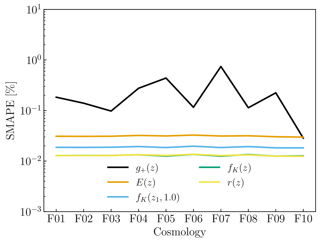
Figure 1: Summary SMAPE values for the comparison of the cosmological functions as obtained by CLOE with those used in LiFE. Notice that we only show the transverse distance $f_{K}(z_{1},z_{2})$ with $z_{2}=1$. We obtained the comparison also with $z\in\left[0.5,1.5,2.0\right]$ obtaining the same results. We do not show these to avoid overlapping lines.

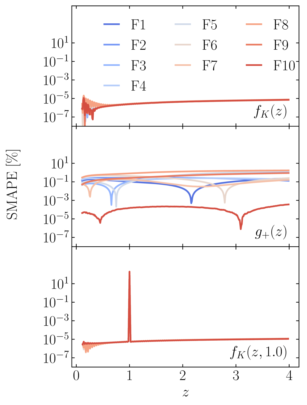
Figure 2: Comparison of the cosmological quantities internally computed by CLOE with those extracted from CAMB for the cosmologies listed in Table 3. Please note that CAMB automatically sets $f_{K}(z_{1},z_{2})=0$ when $z_{1}>z_{2}$, while CLOE returns its absolute value for any redshift combination. In order to perform this comparison, we symmetrise the results obtained from CAMB. The spikes visible in the comparison of the $f_{K}(z_{1},z_{2})$ values are due to this function vanishing when $z_{1}=z_{2}$. As in Fig. 1, we only show the transverse distance $f_{K}(z_{1},z_{2})$ with $z_{2}=1$, with the other cases showing the same behaviour.

However, it is important to consider that, while CLOE extracts $E(z)$ and $r(z)$ directly from a Boltzmann solver (either CAMB or CLASS), it computes internally the other quantities. It is therefore necessary to assess the reliability of these computations against what is obtained by Boltzmann solvers. We present this comparison in Fig. 2, where we show, for all cosmologies considered, the SMAPE of the cosmological quantities internally computed by CLOE with respect to those which can be retrieved from CAMB.

We notice that the distance functions $f_{K}(z)$ and $f_{K}(z_{1},z_{2})$ are in very good agreement with those computed by CAMB, with the SMAPE always staying several orders of magnitude below the $1\%$ level. Furthermore, the change in cosmological parameters does not lead to any significant difference in the comparison, as it can be seen by the overlap of the lines corresponding to different cosmologies in Fig. 2. We observe, however, larger differences in the growth factor $g_{+}(z)$. This is because, while CAMB obtains this quantity by solving the differential equation for the matter perturbation $\delta_{\rm m}$, CLOE computes $g_{+}(z)$ by taking the ratio of the matter power spectra at different redshifts and at a reference scale (see Eq. 22 of Paper 1, for details on this calculations). Despite these differences, the comparison still yields results within a $1\%$ accuracy. However, a revised version of CLOE will aim at further improving this comparison by extracting also this quantity directly from Boltzmann solvers through Cobaya.

It is important to stress that throughout this validation we use CLOE interfaced with CAMB. As discussed in Paper 2, CLOE can also be interfaced with CLASS. However, at the time when our comparison is performed, our baseline recipe for nonlinear corrections, HMCode2020 (Mead et al. 2021), is not available in CLASS, making it impossible to apply the full validation pipeline by interfacing CLOE with CLASS. Nevertheless, we show in Appendix C a comparison between the main cosmological quantities used in the calculation of theoretical predictions between CLOE + CLASS and CLOE + CAMB.

5.2 Photometric 3×2pt observables

In this section, we apply our validation methodology to the observables and intermediate quantities related to the photometric survey of Euclid. We divide this validation into three classes of functions to be compared: kernel functions, power spectra, and photometric observables (see Sect. 3 of Paper 1, ). In this section, we show the validation results across the cases described in Sect. 3, highlighting the overall comparison of these quantities. We report in more detail the validation of a specific case in Appendix A.

The first set of intermediate quantities that we focus on are the kernel functions entering the expression for photometric observables, namely the shear kernel $W^{\gamma}_{i}(z)$, the magnification kernel $W^{\mu}_{i}(z)$, the galaxy kernel $W^{\rm g}_{i}(z)$, and the intrinsic alignment kernel $W^{\rm IA}_{i}(z)$.

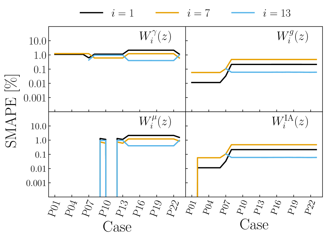
Figure 3: Summary SMAPE values for the kernels comparison between CLOE and LiFE in the different cases investigated. Each colour refers to a different redshift bin of the tomographic Euclid analysis. The figure shows the comparison result in each case for representative redshift bins at low ($i=1$, black lines), intermediate ($i=7$, orange lines) and high redshift ($i=13$, cyan lines). Notice that for the cases P01 to P06 this latter bin is not available, as the $n(z)$ is divided in only 10 tomographic bins. The specifications of the different cases are reported in Table 2.

We report the overall value of the SMAPE for the four kernels in Fig. 3. Here we can notice how the SMAPE values are of the order of one per cent, with $W^{\gamma}_{i}$ and $W^{\mu}_{i}$ being the kernels with the worst agreement. This deviation is caused by the fact that the calculation of these functions requires an integration of the binned galaxy redshift distribution (see Paper 1, ); if such a distribution is not smooth, differences in the numerical sampling between the codes can propagate to the final kernel computations. Indeed, it can be noticed how the cases P01–P06 yield a generally better comparison, as these cases assume the ISTF galaxy redshift distribution (Euclid Collaboration: Blanchard et al. 2020), which is more regular and with broader bins with respect to the other two, limiting the impact of numerical errors.

Following the validation of the kernel functions, we shift our attention to the power spectra entering the calculation of the photometric observables (see section 3.1 of Paper 1, ). These are the matter power spectrum $P_{\rm m}(k,z)$, the galaxy power spectrum $P_{\rm gg}(k,z)$, and the intrinsic alignment power spectrum $P_{\rm II}(k,z)$, together with all cross combinations $P_{{\rm gm}}$, $P_{{\rm gI}}$, and $P_{{\rm mI}}$.

We report the overall value of the SMAPE for the six power spectra, computed at four different redshifts, in Fig. 4. It is possible to notice how the comparison does not exhibit a strong case dependency, with mostly constant trends for the SMAPE values at all redshifts and for all spectra. Nevertheless, it is possible to see a dependency on the chosen case for the P13–P22 cases, where the cosmological parameters change in value, in the power spectra containing the intrinsic alignment contribution. This trend can be connected to the differences between the two codes in the growth factor $g_{+}(z)$, discussed in Sect. 5.1.

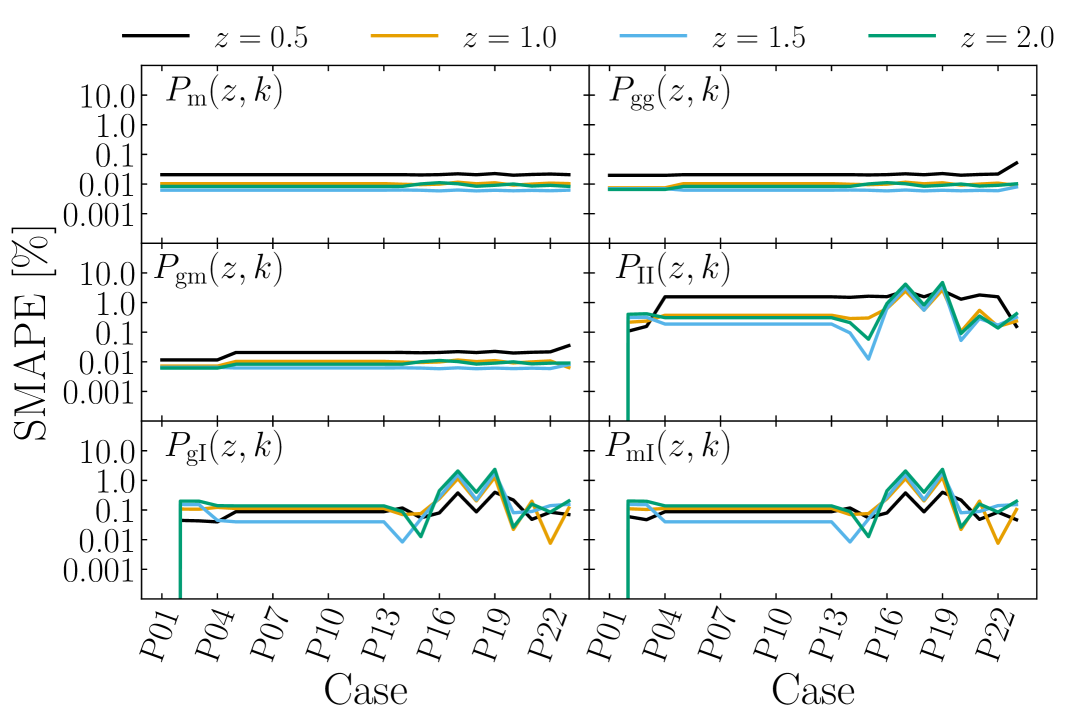
Figure 4: Summary comparison for the intermediate power spectra, as computed by CLOE and LiFE. For each of the different power spectra, shown in separate panels, we show the comparison at different redshifts. The specifications of the different cases are reported in Table 2.

Now that we have assessed the agreement on the intermediate quantities, we focus on the final photometric observables, namely the $C^{AB}_{ij}(\ell)$ power spectra in all observables and redshift bin combinations.

In Fig. 5, we show in the left panel the mean and maximum distances for each of the validation cases, while in the right panel we report the value of the reduced $\chi^{2}$ (solid lines), obtained by dividing the results of Eq. 6 by the number of degrees of freedom ($N_{\rm dof}$) corresponding to each case. We show the trend of such a quantity for the two photometric observables (WL and GCph), their cross-correlation (GGL), and, for the $\chi^{2}$ calculation, their combination (3$\times$2pt). We find that, in all validation cases, both the distance in units of the expected error and the reduced $\chi^{2}$ fall within the threshold values, highlighting the statistical compatibility of the theoretical predictions of CLOE with those of the benchmark code.

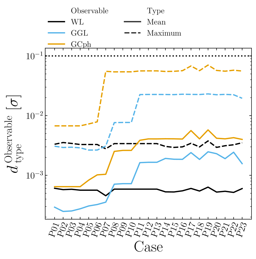
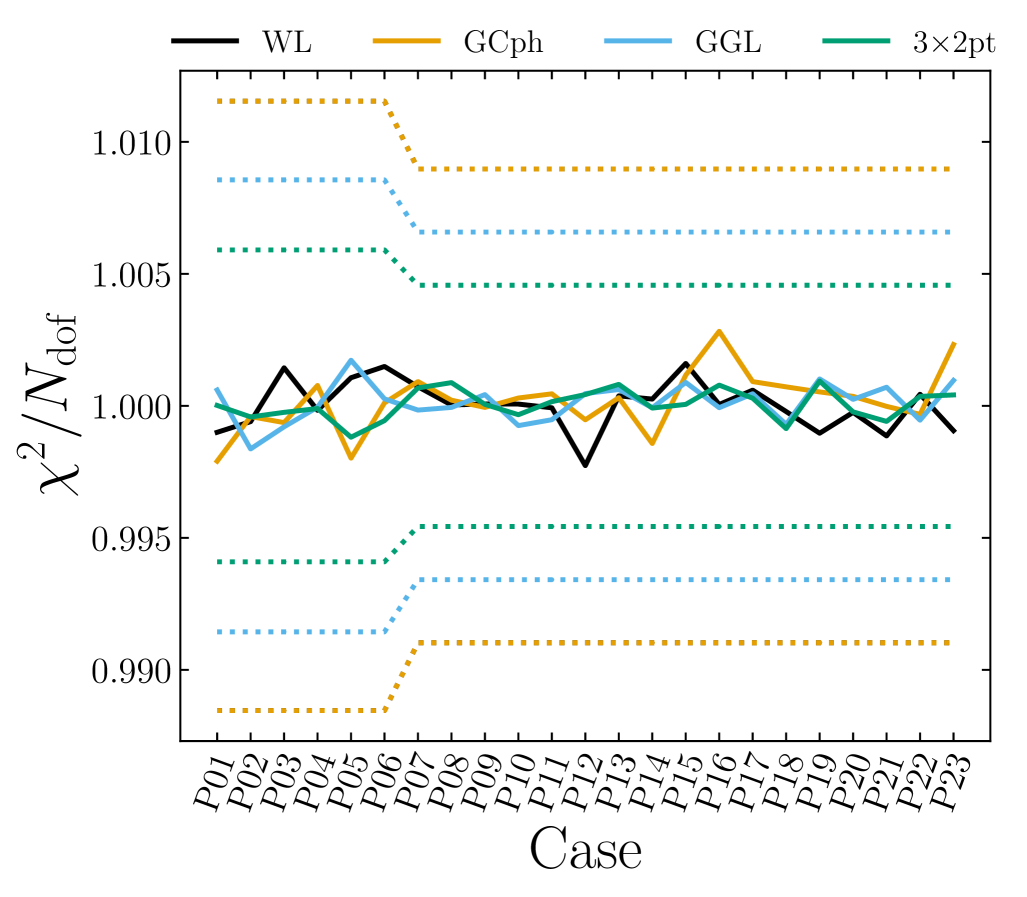
Figure 5: Left panel: distance in units of the expected error for the three photometric observables, both when averaged over the multipoles (solid lines) and taking the highest value of the distance (dashed lines). The black dotted line indicates our threshold of $d=0.1\,\sigma$. Right panel: the solid lines show the average reduced $\chi^{2}$ value for WL (black), GCph (orange), GGL (cyan), and their combination (green). The dashed lines represent the limiting values of the reduced $\chi^{2}$ corresponding to the chosen probability threshold. The results are shown for the different cases described in Table 2.

We notice how all observables exhibit a better agreement for the P01–P06 cases. This is due to the fact that these cases assume the galaxy distribution of ISTF, that is a distribution that is split into fewer bins and whose functions are much smoother than in other validation cases. This allows us to reduce numerical and interpolation errors with respect to other galaxy distributions when computing the kernel functions, thus yielding a better comparison. Overall, we find no significant discrepancy between the benchmark and the predictions of CLOE, independently of the observable analysed or of the validation case.

5.3 Spectroscopic galaxy clustering observable

In this section, we validate the implementation of the model relevant for the spectroscopic probe of Euclid. The validation of intermediate quantities, such as the individual contributions entering the perturbative expansion of the reference nonlinear model implemented in CLOE, will be presented in a dedicated paper (Euclid Collaboration: Crocce et al. 2025). Here, we restrict our analysis to the final spectroscopic observables, namely the Legendre multipoles $P_{\ell}(k,z)$ of the anisotropic galaxy power spectrum.

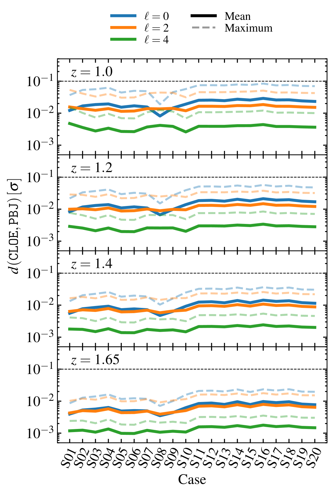
Figure 6: Maximum relative difference between CLOE and PBJ in units of a Gaussian standard deviation obtained with the configuration described in Sect. 4.2. Different panels correspond to different redshifts, as shown in the corresponding top left corners. Different multipoles are identified by the different colours, while solid and dashed lines mark the average and maximum difference along the sampled $k$ values, respectively. The dotted horizontal line in each panel marks the threshold of $10\%$ of the statistical error.

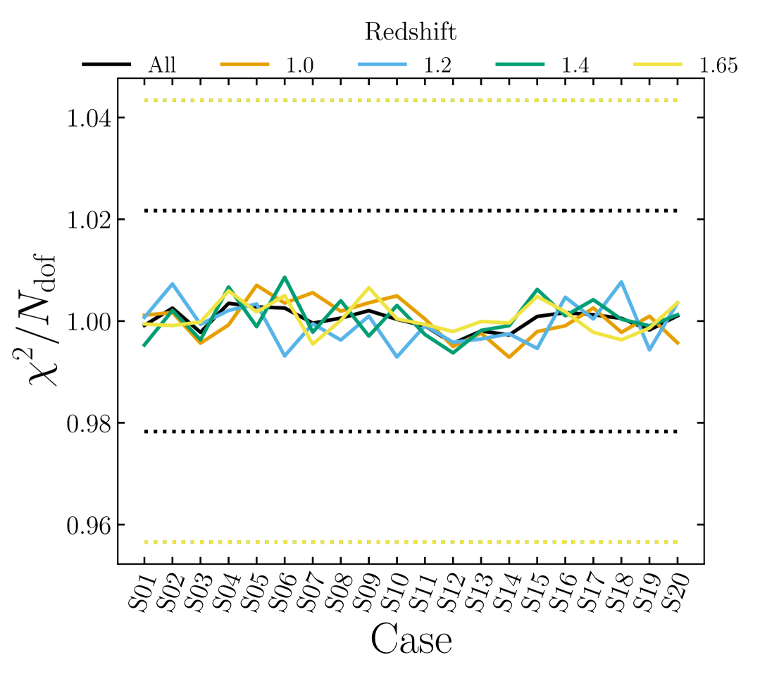
Figure 7: Averaged reduced $\chi^{2}$ displayed in the 20 validation cases for the GCsp probe combination. As in Fig. 5, the dotted lines show the limiting 68-th percentile of the corresponding $\chi^{2}$ distribution with the same number of degrees of freedom, assuming the covariance matrices described in Sect. 3.

The main results of the validation are presented in Fig. 6. Here we show the distance metrics between CLOE and PBJ as defined in Eqs. 4 and 5, considering all redshift bins, multipole orders, and validation cases. Since the recipe for the anisotropic galaxy power spectrum $P_{\rm gg}(k,\mu)$ in CLOE follows the same implementation as in PBJ, we find a good match between the two sets of predictions, with a relative error that always stays below 10% of the statistical error. This happens not only when considering the mean distance between the two sets of predictions but also with the maximum distance. Given this level of agreement, the averaged reduced $\chi^{2}$ values obtained by comparing the theory vectors generated by CLOE and PBJ are also extremely good, as we show in Fig. 7. Quantitatively, the average $\chi^{2}$ lies entirely within the $68\%$ confidence region of the corresponding $\chi^{2}$ distribution with the same number of degrees of freedom. Residual fluctuations are primarily due to differences in the unit conventions adopted by the two codes (i.e. choosing $\mathrm{Mpc}^{-1}$ against $h\,\mathrm{Mpc}^{-1}$), which can induce small discrepancies in the computation of the internal components of the loop expansion, as well as in the algorithms used to project the 2D power spectrum onto the Legendre polynomials.

While this section focuses only on the distance metrics and averaged $\chi^{2}$ statistics, a direct comparison of the theory vectors for a reference case is presented in Appendix A.2.

6 Comparison of real-space correlation functions

In Sect. 5.2 and Sect. 5.3, we assessed the validity of CLOE focusing on the harmonic-space power spectra $C^{AB}_{ij}(\ell)$ and the Legendre multipole $P_{\mathrm{obs},\ell}(k^{\mathrm{fid}},z)$ as the observables to be compared. However, several analyses of LSS data in the literature rely instead on the two-point correlation functions in real space. For the photometric survey, these are the galaxy correlation function $\xi^{\rm GG}_{ij}$, the two lensing correlations $\xi^{+}_{ij}$ and $\xi^{-}_{ij}$, and the galaxy-galaxy lensing correlation $\xi^{\rm GL}_{ij}$, while for the spectroscopic survey we are interested in the 2PCF Legendre multipoles $\xi_{{\rm obs},\ell}(s^{\rm fid},z)$.

In the comparison performed in Sect. 5 we relied on the intuitive definition of distance defined in Eq. 3, obtaining the error $\sigma_{O_{i}}$ from the diagonal of the covariance matrices. However, this requires the off-diagonal terms in the covariances to be negligible, which is not the case for 2PCF (see e.g. Eisenstein & Zaldarriaga 2001). This can be easily observed in Figs. 8 and 9, where we show the correlation matrix for the photometric and spectroscopic cases.

This implies that the error obtained by taking the diagonal of these matrices would yield a significant underestimation of the uncertainties with respect to what would be obtained by considering the full covariances. For such a reason, in comparing the photometric and spectroscopic 2PCF we will rely only on the $\chi^{2}$ estimate of Eq. 6, avoiding the computation of the distance in units of the error.

Furthermore, CLOE computes the 2PCF by projecting the observables validated in Sect. 5. For such a reason, we do not repeat the validation for all the cases discussed in Sect. 3, deeming it sufficient to perform the validation in the reference cases, P23 and S01 for the photometric and spectroscopic surveys, respectively.

For the photometric correlation functions, we perform the validation by computing the covariance matrix using the public OneCovariance code (Reischke et al. 2024). This computes the covariance in harmonic space and then projects it to real space using the equations presented in Joachimi et al. (2021).

For the spectroscopic correlation functions, similarly to the case in Fourier space, we only make use of the Gaussian limit, which translates to a conservative validation of the implementation in CLOE. In this case, the covariance matrices for the four different spectroscopic bins have been computed using the public GaussianCovariance code.

We present the results of our comparison in Table 4, where it is possible to notice how the reduced $\chi^{2}$ value obtained for the 2PCF are within the expected limits for both the photometric and spectroscopic surveys.

Table 4: Reduced $\chi^{2}$ and its limiting inferior (inf) and superior (sup) values for a probability threshold of 68%.

	Photometric
	$\xi^{\rm GG}_{ij}$	$\xi^{\rm GL}_{ij}$	$\xi^{-}_{ij}$	$\xi^{+}_{ij}$
inf	0.977	0.983	0.977	0.977
$\chi^{2}/N_{\rm dof}$	1.021	0.999	1.000	1.001
sup	1.023	1.017	1.023	1.023
	Spectroscopic
	$z=1.0$	$z=1.2$	$z=1.4$	$z=1.65$
inf	0.902	0.902	0.902	0.902
$\chi^{2}/N_{\rm dof}$	0.999	0.999	1.001	0.997
sup	1.097	1.097	1.097	1.097

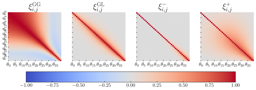
Figure 8: Correlation matrices between the different angles $\theta_{i}$ for which the 2PCFs are computed, taken for $i=j=6$ in the P23 case.

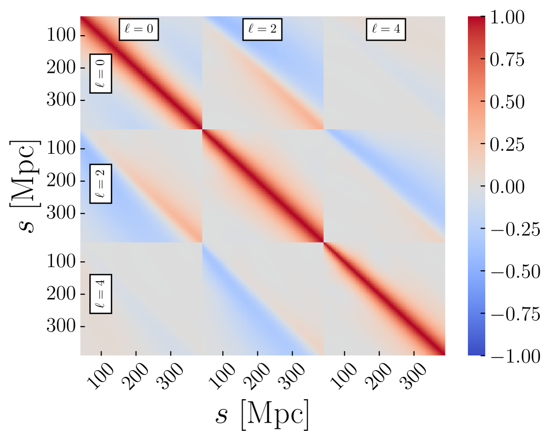
Figure 9: Correlation matrix of the linear-theory 2PCF multipoles assuming the setup adopted for the validation, thus linear bias and RSD signal, and number density corresponding to the ones defined in Paper 3.

7 Conclusions

The main objective of this work was to benchmark the code used to obtain theoretical predictions for Euclid observables: CLOE. In order to do so, we compared such predictions with those obtained from external softwares that implement the same recipe.

While we do not explore systematically the parameter space, we perform this benchmarking in a wide set of validation cases, described in Sect. 3. This allows us to test the features implemented in CLOE, which are described in detail in Paper 1.

After presenting the methodology to quantify the discrepancy between CLOE and the benchmark in Sect. 4, and the external codes used as benchmarks in Sect. 2, we compared as a first step the basic cosmological ingredients of our recipe in Sect. 5.1. Here we found a sub-per cent agreement between CLOE and LiFE for all functions in all the chosen cosmologies and, even more importantly, we found a very good agreement between CLOE and CAMB. For the latter comparison, we found that the most significant difference is obtained for the growth factor $g_{+}(z)$; the internal calculation of CLOE approximates this with the square root of a ratio of matter power spectra which, when compared with the CAMB prediction, yields a discrepancy of one per cent.

Following the validation of these fundamental ingredients, we focused separately on the two surveys of Euclid: spectroscopic and photometric.

In Sect. 5.3, we discussed the validation of the final spectroscopic observables against an external code, PBJ, which implements the same model for the spectroscopic galaxy power spectrum based on the EFTofLSS framework. For this comparison, we only considered the final Euclid observables, the power spectrum Legendre multipoles, while we left the benchmarking of intermediate quantities to a dedicated work (Euclid Collaboration: Crocce et al. 2025; Euclid Collaboration: Moretti et al. 2025) We computed a distance metric between the two codes based on a Euclid-like statistical uncertainty that assumes only the Gaussian limit, therefore providing a much more conservative comparison than if also including non-Gaussian contributions. We found an optimal agreement between CLOE and PBJ, with a distance metric that stays consistently below the ten per cent of the expected statistical error for all redshifts and wavemodes. Furthermore, the $\chi^{2}$ analysis shows that the theoretical predictions of CLOE are in statistical agreement with the dataset generated using PBJ.

The validation of the photometric observables was presented in Sect. 5.2, where, in addition to the final observables for this survey, we also validated the implementation of intermediate calculations. As a first step, we looked at the kernel functions $W^{A}_{i}(z)$, which contain the galaxy redshift distribution $n_{i}(z)$ for each redshift bin $i$, and enter the integrals for the power spectra. We found that these functions agree with the benchmarking code within approximately one per cent, with the comparison getting worse the less smooth the $n_{i}(z)$ distributions are (see Fig. 3).

The other ingredients entering the calculation of $C^{AB}_{ij}(\ell)$ are the power spectra for galaxies, matter and intrinsic alignment. We found these functions to be compatible with the benchmark well within one per cent, with the worst performance found for the power spectra containing the intrinsic alignment terms, which are those related to the growth factor $g_{+}(z)$. We have shown these comparisons in Fig. 4.

With these quantities validated, we moved to the final observables computed by CLOE, the power spectra $C^{AB}_{ij}(\ell)$. As described in Sect. 4, we assess the compatibility between CLOE and the benchmark (LiFE) by computing the distance between their predictions in units of the expected error, as well as fitting the predictions of the former to a simulated dataset generated using the latter. We show in Fig. 5 how in all our validation cases both the distances and the reduced $\chi^{2}$ are well within its limiting values for the chosen probability threshold ($68\%$). We find no significant difference for the separate photometric observables or their combination, as well as no significant trend with the analysed cases, except for a better agreement found in the case P01–P06, where we use a smooth galaxy distribution. Thus, we can conclude that the harmonic power spectra of CLOE are statistically compatible with the benchmark within the expected DR3 errors of Euclid.

In Appendix A, we have shown a more detailed comparison specifying to a single case. For the photometric observables, we chose the P23 case as a reference, showing in Fig. 10 the distance in units of the observational errors as a function of the multipole $\ell$, for each observable. Similarly, we show in Fig. 11 the trends in $k$ of the distance for the spectroscopic observables, choosing as a reference the S01 case.

Similarly, the validation of the 2PCF Legendre multipoles points towards an optimal consistency of the implementation present in CLOE with the one produced by COFFE. In this case, given the non-negligible contributions of the off-diagonal terms in the covariance, we only performed the $\chi^{2}$ analysis, reported in Table 4, finding good statistical agreement between CLOE predictions and the benchmark.

In Table 4, we also report the results of the $\chi^{2}$ analysis for the photometric two-point correlation functions, obtained as a projection of the $C^{AB}_{ij}(\ell)$. Also in this case we find good agreement with the benchmark.

Thanks to the results obtained in this paper, we conclude that CLOE is a reliable and accurate software, able to compute Euclid’s main observables efficiently while being in agreement with other software. We are therefore positive that the final results obtained with Euclid will have negligible bias coming from the theoretical calculations we examined in this work.

Appendix A Reference case comparison

In Sects. 5.2 and 5.3 we compare the predictions of CLOE with those of the benchmark in a variety of cases, exploring different features that are available in CLOE. Here, instead, we present in more detail the comparison in a specific case, that is the one used as a fiducial to obtain the results presented in Paper 3.

A.1 Photometric survey

For the photometric survey, we choose as a reference the P23 case, and we show in Fig. 10 the trends in multipoles of the distance in units of the error for weak lensing (WL), photometric galaxy clustering (GCph), and their cross-correlation galaxy-galaxy lensing (GGL). We find no significant trend with the multipoles $\ell$ and no significant difference between the analysed probes. We find GCph to be the observable with the highest values of this distance, compatible with the results presented in Sect. 5.2, which is a direct result of the smaller observational error for this observable with respect to the others.

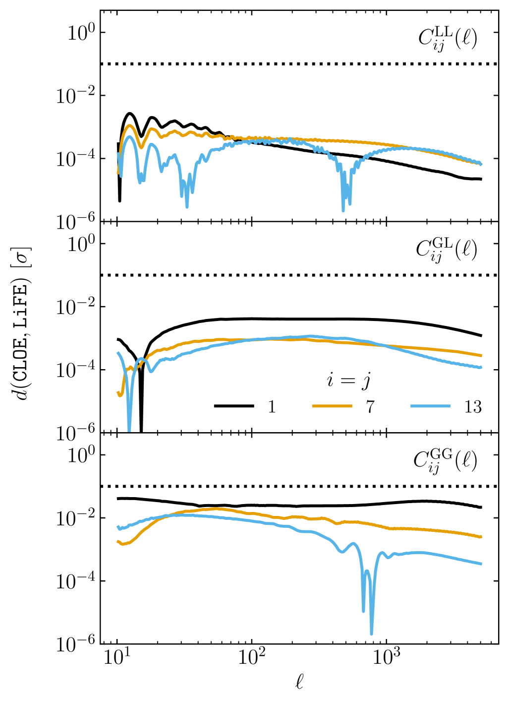
Figure 10: Distance in units of the expected error as a function of the multipole $\ell$ for WL (top panel), GCph (middle panel), and their cross-correlation GGL (bottom panel). The different colours indicate the redshift bin considered. The black dotted line shows the threshold value of $0.1\,\sigma$. This comparison is performed in the reference case P23.

A.2 Spectroscopic survey

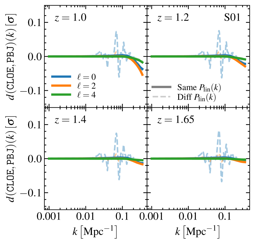
Figure 11: Systematic difference between CLOE and PBJ for the case S01 (flat $\varLambda\mathrm{CDM}$) of GCsp. The difference is quantified in terms of the distance metric defined in Eqs. (5-4). Different colours correspond to different multipoles, while solid and dashed lines denote the case when CLOE and PBJ use the same input linear power spectrum or not, respectively.

In Fig. 11, we show the distance metric as a function of the wavemode $k$ for a reference case, a flat $\varLambda\mathrm{CDM}$ cosmology as in case S01. In all panels, we show the accuracy between CLOE and PBJ using two sets of predictions: in the first one, each code obtains the linear power spectrum predictions from an individual call to the Boltzmann solver (CAMB in this case), while, in the second one, the same linear predictions are used consistently across the two codes. In the first case, we observe residuals in the final Legendre multipoles that are anyway always smaller than 10% of the corresponding statistical error for a few spurious positions along the $k$ axis, mostly concentrated over the BAO scales. This is a consequence of employing slightly different versions and accuracy flags in the Boltzmann solver, but despite this difference, the trend is to have an optimal consistency in terms of the broadband of the multipoles. The agreement is even better when considering the same input spectra, for which we only observe a minor deviation at $k\gtrsim 0.1\,{\rm Mpc}^{-1}$ that are induced by a small difference in the way infrared resummation is carried out in the two codes. This is mostly due to the different set of units adopted by the two codes, with or without $h$, respectively (Euclid Collaboration: Moretti et al. 2025).

Appendix B Comparison with CCL

The comparison against CCL has proceeded as described above for LiFE. To compute the final observables of interest (2PCF and power spectra), the code requires as external input the $n(z)$, the tabulated values of galaxy and magnification bias, and the tabulated IA kernel. The $C^{AB}_{ij}(\ell)$ are then computed, using the Limber approximation, using quadrature integration (which is the most accurate and for which the best agreement is found) as mentioned in Sect. 2.1.2. To be as accurate as possible, we boost some of the accuracy settings, such as the number of points in $z$ and $k$ used for the power spectrum splines and the number of points at which the kernels are evaluated.

The results of the comparison, shown in Fig. 12, are below the $0.1\,\sigma$ threshold for all the cases investigated, which as mentioned above are all the cases without RSD.

Generally, the distance between CLOE and CCL increases with the complexity of the source and lens redshift distribution, as is also the case for the comparison against LiFE (see Fig. 5); this is an expected result, and is more prominent for GCph since the relative kernels are much less smooth and have narrower support. The few cases above the threshold are indeed only for the maximum GCph discrepancy, and only concern individual or very small sets of $\ell$ values. As it can be seen in the bottom panel of Fig. 5, such differences do not lead to statistical incompatibilities.

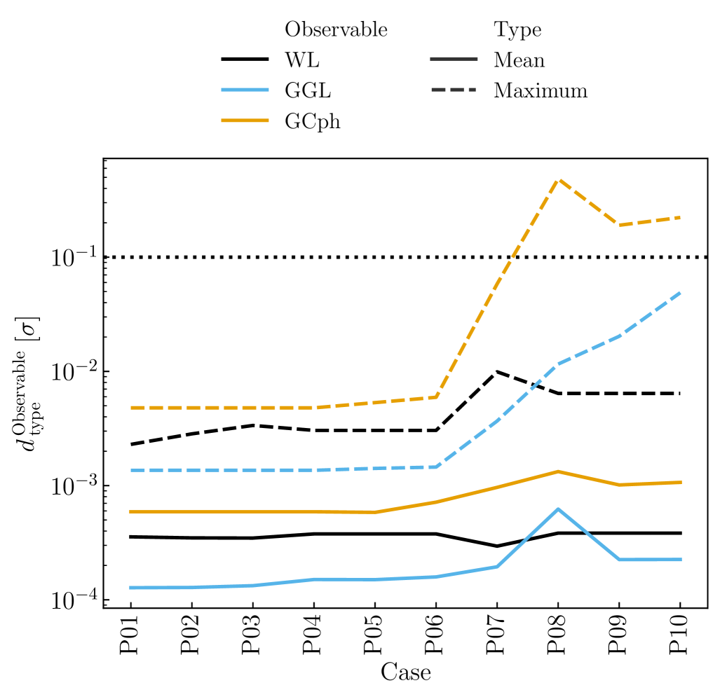
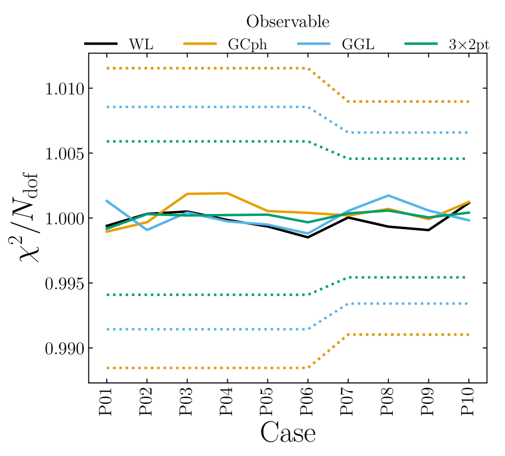
Figure 12: Equivalent of Fig. 5 using CCL as a benchmark.

Appendix C Cosmology with CLOE + CLASS

The results and main conclusions that we draw in this work are obtained using CLOE interfaced to the Boltzmann solver CAMB, through the structure of Cobaya (see Paper 2, ). However, CLOE has been built having in mind the possibility of switching between CAMB and CLASS without anything significant change in the pipeline.

At the time of this comparison, the version of CLASS interfaced does not allow us to use the nonlinear recipe we identified as our baseline choice (HMCODE2020), and therefore we cannot apply to the CLOE + CLASS configuration the same validation pipeline we used for CLOE + CAMB.

Nevertheless, the calculations performed by CLOE are independent of the choice made on the Boltzmann solver, on which the code relies only to obtain a set of basic cosmological ingredients, used in the calculations. For such a reason, in order to assess the agreement between CLOE + CAMB and CLOE + CLASS, it is enough to compare these functions in the two cases, as all subsequent calculations will be identical, whatever the choice for the Boltzmann solver is.

These basic cosmological ingredients necessary for CLOE are:

• the normalised Hubble rate $E(z)\equiv H(z)/H_{0}$;

• the comoving distance $r(z)$;

• the linear matter power spectrum $P_{\rm m}^{\rm LIN}(k,z)$.

Through these functions, CLOE computes other derived cosmological quantities, such as the growth factor $g_{+}(z)$ and the growth rate $f(z)$, and later combines them all together to compute the observables (for details, see Paper 1, ). While the linear matter power spectrum $P_{\delta\delta}^{\rm LIN}$ is not used directly in any calculation, this is the input for the nonlinear methods used in CLOE, and therefore it constitutes one of the relevant cosmological quantities.

In Fig. 13, we show the SMAPE obtained for these four main functions, with the comparison for the last function performed at four different values of the redshift.

We find no significant difference in these functions when switching between the two Boltzmann solvers, with all the differences being at most at the level of one per cent. Such a result is not surprising, given that the structure choices made in developing CLOE were also aimed at removing any dependence on the choice of the solver. Nevertheless, the results found highlight how also in the part of the code that directly interfaces with the Boltzmann solvers the differences are not significant.

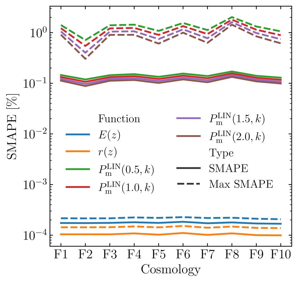
Figure 13: Summary SMAPE values for the comparison between the cosmological function extracted from the Boltzmann solver in the CLOE +CAMB and CLOE +CLASS configurations.