Training Feature Attribution for
Vision Models

Abstract

Deep neural networks are often considered opaque systems, prompting the need for explainability methods to improve trust and accountability. Existing approaches typically attribute test-time predictions either to input features (e.g., pixels in an image) or to influential training examples. We argue that both perspectives should be studied jointly. This work explores training feature attribution, which links test predictions to specific regions of specific training images and thereby provides new insights into the inner workings of deep models. Our experiments on vision datasets show that training feature attribution yields fine-grained, test-specific explanations: it identifies harmful examples that drive misclassifications and reveals spurious correlations, such as patch-based shortcuts, that conventional attribution methods fail to expose.

1 Introduction

Deep neural networks have achieved state-of-the-art performance across a wide range of domains, including image recognition, natural language processing, and multimodal reasoning (He et al., 2016; Devlin et al., 2019; Radford et al., 2021). However, this impressive performance comes at the cost of transparency: modern deep models operate as complex, highly-parameterized black boxes, where the reasoning behind individual predictions is often opaque (Lipton, 2018). This opacity can undermine user trust, hinder debugging, and conceal harmful biases or spurious correlations (Arjovsky et al., 2019; DeGrave et al., 2021). In high-stakes applications such as healthcare, finance, or autonomous systems, understanding why a model makes a specific decision is as important as the decision’s accuracy itself (Rudin, 2019; Doshi-Velez & Kim, 2017). Explainability methods aim to bridge this gap by attributing model predictions to interpretable causes, enabling practitioners to verify alignment with domain knowledge, detect potential failures, and ensure accountability. This is also a way to improve interaction between humans and AI systems (Wickramasinghe et al., 2020).

Within the literature on eXplainable AI (XAI), two main attribution paradigms can be distinguished: feature attribution (FA), which highlights the parts of a test input most responsible for its prediction (e.g., pixels in image classification), and training data attribution (TDA), which identifies the training examples most influential for a given test prediction.

While both provide valuable insights, each has inherent limitations. Feature attribution ignores where in the training data the model learned its decisive features, while TDA ignores what aspects of those examples matter most (see Figure 3). For instance, a feature attribution map might highlight a “striped” region in a zebra image without indicating whether the stripes were learned from zebras or from unrelated patterns in the training set; conversely, TDA might flag a specific training image without clarifying which region of it was influential.

This gap motivates training feature attribution (TFA), a framework that connects test predictions to specific regions of training examples. By combining TDA with FA, such an approach enables us to answer the question, Which parts of which training images are most responsible for the model’s decision on this test image?

figureb[floatrow]floatrowcapbesideposition=right,top,capbesidewidth=.38floatbesidecapbesidefloatfigurebesidecapbesidefigureb[floatrow]floatrowcapbesideposition=right,top,capbesidewidth=.38floatbesidecapbesidefloatfigurebesidecapbesidefigureb [floatrow]floatrowcapbesideposition=right,top,capbesidewidth=.38floatbesidecapbesidefloatfigurebesidecapbesidefigureb Figure 3: A prediction on a test example depends both on the features of the example, as well as on features learned from the training examples through the trained parameters.

Related works

While feature attribution and training data attribution have each been extensively studied in isolation, there has been comparatively little research on integrating these approaches into a unified framework. A notable exception is the exploration of training feature attribution within natural language processing (NLP) for artifact discovery (Han et al., 2020; Pezeshkpour et al., 2021), as well as token-wise influence functions in large language models (Grosse et al., 2023). We build upon these efforts by extending the framework to vision data, where the notion of ”features” is inherently less well-defined. Unlike tokens in NLP, which typically carry semantic meaning individually, pixels in images convey limited information in isolation and gain significance primarily through their spatial interactions with other pixels.

For vision tasks, other related efforts include concept-based attribution methods, which decompose model activations into human-interpretable concepts (Kim et al., 2018); prototype-based explanations, such as ProtoPNet (Chen et al., 2019), which connect predictions to similar image regions; and Visual-TCAV (De Santis et al., 2024), which integrates the TCAV framework (Kim et al., 2018) with saliency maps for predefined concepts. In a different context, the concept of computing pixel-wise influence can be traced back to the seminal work of Koh & Liang (2017), who first applied classical influence functions to deep learning. In their work, it was used as a way to create data poisoning; however, its potential as an explainability tool was not recognized.

Contributions

• We introduce training feature attribution of vision models, and propose a practical algorithm for estimating saliency maps (Section 3). This algorithm is quantitatively validated by masking training images and retraining (Section 4.3);

• We introduce a simplified analytical setup where the TFA method correctly recovers the important training feature for a given test example (Section 3.1);

• We present 2 practical use cases where TFA is more insightful for debugging trained deep neural networks than using only TDA or FA (Section 5).

2 Background : Attributing predictions to either features or training data

2.1 Training Data Attribution

Example-based explanation methods (surveyed in Poché et al., 2023) offer a natural way to interpret machine learning models, where explanations are conveyed through representative samples rather than abstract feature scores. This paradigm aligns with human reasoning, as people often justify decisions by referring to familiar cases: “This looks like something I’ve seen before.” It reflects cognitive processes in which new observations are understood by comparison with previously encountered examples, allowing concepts to be formed through such comparisons (Miller, 2019; Byrne, 2016; Gentner, 1983).

Within this family, various strategies exist: prototype methods select representative instances from the data (Chen et al., 2019); concept-based methods (Kim et al., 2018; Fel et al., 2023) explain predictions in terms of higher-level semantic factors; and criticisms, or irregular instances, highlight unusual or atypical cases in the data (Kim et al., 2016).

Another form of example-based explanation is training data attribution (TDA), which aims to trace a model’s prediction back to the training examples that most influenced it. Each training instance is assigned an importance score reflecting its effect on the model’s behavior for a specific test case. A positive score indicates that the example supported the prediction by pushing it toward the correct label, while a negative score means it opposed the prediction, pulling it toward an incorrect outcome.

TDA approaches vary in how they estimate influence. Influence function-based methods (Koh & Liang, 2017) compute the hypothetical effect of upweighting or removing an example at training time. Approaches based on gradient or representation similarity estimate influence by comparing the model’s response to training and test inputs (Charpiat et al., 2019; Hanawa et al., 2021; Pruthi et al., 2020). Game-theoretic frameworks such as DataShap (Ghorbani & Zou, 2019) approximate Shapley values to assign each training point a contribution score.

Mathematical Formulation

Consider a supervised classification problem with a training set $\mathcal{D}_{\text{train}}=\{z_{i}^{\text{train}}\}_{i=1}^{N}$ and a test set $\mathcal{D}_{\text{test}}=\{z_{j}^{\text{test}}\}_{j=1}^{M}$, where $z=(x,y)$ denotes an input-label pair. A trained model $f_{\theta}$ is obtained by searching parameters $\hat{\theta}$ that minimize the empirical risk:

$$\hat{\theta}=\mathop{\mathrm{argmin}}_{\theta}\ \frac{1}{N}\sum_{i=1}^{N}\ell(f_{\theta}(x_{i}^{\text{train}}),y_{i}^{\text{train}})$$

where $\ell$ is the loss function. At the end of training, the predictor $f_{\hat{\theta}}$ is therefore influenced by all examples $z_{i}^{\text{train}}$ seen during training.

A training data attribution method assigns an importance score $S(z_{i}^{\text{train}},z_{j}^{\text{test}})$, measuring the effect of including a particular training point $z_{i}^{\text{train}}$ on test predictions of the trained model $f_{\hat{\theta}}(x_{j}^{\text{test}})$ or their losses. These scores can be positive for training points that support the test label $y_{j}^{\text{test}}$, or negative for training examples that oppose the current label, which for instance happens when a training example is considered similar to the test example by the model, but labeled as a different class. Ranking training points by their TDA score $S(\cdot,z_{j}^{\text{test}})$ provides insight into which training instances most influenced (both positively and negatively) the model’s decision for a given test example.

2.2 Feature attribution

Feature attribution (FA) methods aim to explain a model’s prediction for a given test input by assigning an importance score to each input feature (e.g., pixels in an image). Unlike data attribution, which seeks to identify influential training examples, feature attribution answers: Which parts of the input were most responsible for this prediction? This is especially useful for extracting more interpretable rules from trained deep neural networks, where the gigantic number of individual parameters renders the behavior of the model difficult to interpret.

Early approaches to feature attribution include the deconvolutional network method and occlusion sensitivity analysis (Zeiler & Fergus, 2014), as well as simple gradient-based saliency maps that highlight input regions most relevant to a class prediction (Simonyan et al., 2013). More recent methods fall into two broad families: perturbation-based and gradient-based. Perturbation-based methods, such as LIME (Ribeiro et al., 2016) and SHAP (Lundberg & Lee, 2017), measure the effect of systematically masking or altering input features to estimate their importance. LIME approximates the model locally with an interpretable surrogate, while SHAP employs Shapley values from cooperative game theory to attribute contributions to each feature.

Gradient-based methods instead rely on the derivatives of the model’s output with respect to its input. Examples include Integrated Gradients (Sundararajan et al., 2017), which accumulates gradients along a path from a baseline to the input, and SmoothGrad (Smilkov et al., 2017), which averages gradients computed on noisy versions of the input to improve robustness. For convolutional networks (CNNs) applied to vision tasks, techniques such as Grad-CAM (Selvaraju et al., 2017) and Grad-CAM++ (Chattopadhay et al., 2018) generate visual explanations by highlighting the spatial regions of an image most influential for a specific class prediction.

Despite their popularity, recent work shows that saliency methods can be misleading: they may produce similar maps even after randomly resampling model parameters or permuting labels, passing visual ‘sanity checks’ while not reflecting what the model actually learned (Adebayo et al., 2018).

3 Approach: attribution of test-time predictions to features seen during training

From a learning-theoretic perspective, the features used at test time in trained deep networks are learned entirely from the training set (Figure 3). A model cannot reliably assign importance to a feature it has never observed during training; for example, if most cow images in the training data show grassy fields, the model may misclassify a cow in a desert as a camel, even if the cow is clearly visible to a human observer (Arjovsky et al., 2019; Beery et al., 2018). As an ideal long term goal, we would like to have an explainability tool able to surface these implicit mechanisms in terms of high level features.

While both FA and TDA offer valuable insights, neither is complete on its own: feature attribution ignores where the model learned those features from, while training data attribution does not reveal which parts of the training examples were most important. Our aim is to combine the strengths of both approaches, creating training feature attribution methods that connect test-time predictions back to specific regions of specific training examples.

3.1 Analytic Toy Example

To make motivation more concrete, we analyze a simple linear ridge regression model in $\mathbb{R}^{2}$ amenable to full analytical treatment (detailed derivation is provided in Appendix A). Define $y=x_{1}+x_{2}$ to be the ground truth rule to learn. We are given a training dataset $\left\{\left(x_{i},y_{i}\right)\right\}_{i\leq n}$ where for $i\in\left\{1,...,n-1\right\}$, examples $x_{i}=(x_{i1},0)$ lie on the canonical $e_{1}$ axis, while a single informative point reveals the signal in the $e_{2}$ direction $x_{n}=(0,c)$ with $c\neq 0$.

TDA

In the closed-form solution to ridge regression, we can compute the exact contribution of each training point to the learned function using the representer decomposition:

$$f_{w^{\star}}(x_{\ast})=\sum_{i=1}^{n}\alpha_{i}y_{i},\qquad\alpha_{i}=x_{\ast}^{\top}(X^{\top}X+\lambda I)^{-1}x_{i}.$$

For a test point $x_{\ast}=(0,t)$, $t\neq 0$, we obtain $\alpha_{i}=\frac{t}{c^{2}+\lambda}\,x_{i2}$, which gives $\alpha_{i}=0$ for $i\neq n$, and $\alpha_{n}y_{n}=\frac{tc^{2}}{c^{2}+\lambda}=f_{w^{\star}}(x_{\ast})$. TDA correctly assigns the entire prediction to the single informative training example $(x_{n},y_{n})$.

TFA

We can decompose this effect even further down to the contribution of individual features in $\alpha_{i}$ coefficients. Let $A=(X^{\top}X+\lambda I)^{-1}$. Then

$$f_{w^{\star}}(x_{\ast})=\sum_{i=1}^{n}y_{i}\sum_{k=1}^{2}\beta_{i,k}\qquad\beta_{i,k}=\,x_{ik}\,(e_{k}^{\top}Ax_{\ast})$$

For our test example $x_{\ast}=(0,t)$, $e_{1}^{\top}Ax_{\ast}=0$, hence $\beta_{i,1}=0$ for all $i$. Meanwhile, $\beta_{i,2}=\frac{t}{c^{2}+\lambda}\,x_{i2}$, thus $\beta_{i,2}=0$ for all $i\neq n$ and $y_{n}\beta_{n,2}=\frac{tc^{2}}{c^{2}+\lambda}=f_{w^{\star}}(x_{\ast})$. TFA would here show that only the $x_{n,2}$ feature of that training example contributes to the prediction for example $x_{\ast}$, while all other features are irrelevant.

This illustrates how TFA refines example-based explanations by identifying not only which training example matters (as would TDA already do), but also which feature within it. In the following sections, we aim to design methods to produce similar TFA scores, at the scale of actual deep vision networks.

3.2 TFA Framework: Attributing TDA Scores to input features

Let $S(z_{i}^{\text{train}},z_{j}^{\text{test}})$ denote a training data attribution method, which quantifies the influence of a training point $z_{i}^{\text{train}}$ on the prediction for a test point $z_{j}^{\text{test}}$. Let $x_{i}^{\text{train}}$ be the training image of $z_{i}^{\text{train}}=(x_{i}^{\text{train}},y_{i}^{\text{train}})$. Feature attribution methods generally attribute a given scalar prediction (e.g., the probability or logit of the predicted class) to specific features from the input of the model. The Training Feature Attribution (TFA) approach is to apply feature attribution to the scalar TDA score instead, thus identifying which regions of the input image $x_{i}^{\text{train}}$ are most responsible for the TDA method to deem a training example helpful or harmful. In order to obtain a practical algorithm, we need to choose a pair of TDA and FA methods.

3.2.1 Choice of TDA method: grad-cos

As a choice of TDA method, we select gradient cosine similarity (grad-cos, Charpiat et al., 2019) as the TDA score, because i) it is computationally efficient compared to influence function based methods that require inverting high dimensional Hessian matrices and ii) more importantly, as shown by Hanawa et al. (2021), grad-cos is the training data attribution method among those evaluated that best satisfies all 3 minimal requirements for similarity-based explanations (the model randomization test (Adebayo et al., 2018), the identical class test, and the identical subclass test), ensuring that the most influential examples it identifies are also meaningful from a human perspective. As an alternative, we also performed experiments with influence functions (Appendix B).

Mathematical Formulation of Grad-Cos Attribution

Following Charpiat et al. (2019), suppose that we want to quantify how a small parameter update that reduces the loss on a training example $z_{i}^{\text{train}}$ affects the loss on a test example $z_{j}^{\text{test}}$. Consider a first-order Taylor expansion:

$$\mathcal{L}(z_{i}^{\text{train}};\hat{\theta}+\delta\theta) \approx\mathcal{L}(z_{i}^{\text{train}};\hat{\theta})+\nabla_{\theta}\mathcal{L}(z_{i}^{\text{train}};\hat{\theta})^{\top}\delta\theta$$

The reduction of the loss at $z_{i}^{\text{train}}$ by a small amount $\varepsilon$ can be achieved by choosing:

$$\delta\theta=-\varepsilon\frac{\nabla_{\theta}\mathcal{L}(z_{i}^{\text{train}};\hat{\theta})}{\left\|\nabla_{\theta}\mathcal{L}(z_{i}^{\text{train}};\hat{\theta})\right\|^{2}}$$

This induces a change in the loss for the test point:

$$\mathcal{L}(z_{j}^{\text{test}};\hat{\theta}+\delta\theta) \approx\mathcal{L}(z_{j}^{\text{test}};\hat{\theta})+\nabla_{\theta}\mathcal{L}(z_{j}^{\text{test}};\hat{\theta})^{\top}\delta\theta$$

$$=\mathcal{L}(z_{j}^{\text{test}};\hat{\theta})-\varepsilon\frac{\nabla_{\theta}\mathcal{L}(z_{j}^{\text{test}};\hat{\theta})^{\top}\nabla_{\theta}\mathcal{L}(z_{i}^{\text{train}};\hat{\theta})}{\left\|\nabla_{\theta}\mathcal{L}(z_{i}^{\text{train}};\hat{\theta})\right\|^{2}}$$

which quantifies the effect of the training example $z_{i}^{\text{train}}$ on the loss at $z_{j}^{\text{test}}$. The sign of this effect indicates whether the example is helpful (reducing the test loss) or harmful (increasing the test loss).

Alternatively, a symmetric cosine-similarity version (Charpiat et al., 2019) is defined as:

$$S_{GC}(z_{i}^{\text{train}},z_{j}^{\text{test}})=\frac{\nabla_{\theta}\mathcal{L}(z_{j}^{\text{test}};\hat{\theta})}{\left\|\nabla_{\theta}\mathcal{L}(z_{j}^{\text{test}};\hat{\theta})\right\|}\cdot\frac{\nabla_{\theta}\mathcal{L}(z_{i}^{\text{train}};\hat{\theta})}{\left\|\nabla_{\theta}\mathcal{L}(z_{i}^{\text{train}};\hat{\theta})\right\|}=\cos\!\Big(\nabla_{\theta}\mathcal{L}(z_{j}^{\text{test}};\hat{\theta}),\nabla_{\theta}\mathcal{L}(z_{i}^{\text{train}};\hat{\theta})\Big)$$ (1)

3.2.2 Choice of FA Method: Gradient-Based Importance

In the following, we focus on gradient-based feature attribution methods, which are computationally more efficient than perturbation-based methods and produce sensible saliency maps (Boggust et al., 2023; Smilkov et al., 2017; Adebayo et al., 2018). To derive a pixelwise influence map from $S_{GC}$, we analyze how small perturbations to individual pixels of the training image affect the attribution score.

Remark that $S_{GC}(\cdot,z_{j}^{\text{test}})$ is differentiable with respect to $x_{i}^{\text{train}}$ as the underlying neural network models and standard loss functions are differentiable with respect to their inputs almost everywhere. Consider a small perturbation $\delta\in\mathbb{R}^{d}$ applied to $x_{i}^{\text{train}}$. A first-order Taylor expansion gives:

$$S_{GC}(x_{i}^{\text{train}}+\delta,z_{j}^{\text{test}})\approx S_{GC}(x_{i}^{\text{train}},z_{j}^{\text{test}})+\delta^{\top}\nabla_{x_{i}^{\text{train}}}S_{GC}(x_{i}^{\text{train}},z_{j}^{\text{test}})$$

where $\nabla_{x_{i}^{\text{train}}}S_{GC}(x_{i}^{\text{train}},z_{j}^{\text{test}})$ is the gradient of the attribution score with respect to the training image. This gradient assigns an importance score to each pixel, indicating how sensitive the attribution score is to small changes at that location, which we use as saliency map:

$$\mathrm{Saliency}:=\nabla_{x_{i}^{\text{train}}}S_{GC}(x_{i}^{\text{train}},z_{j}^{\text{test}})$$ (2)

We can further render these heatmaps more visually appealing by additionally applying SmoothGrad (Smilkov et al., 2017) to the saliency map (details in Appendix C).

4 Experiments

4.1 Pixelwise Influence Attribution

We use the Pascal VOC 2012 dataset (Everingham et al., 2015), which contains images from 20 object categories, including vehicles, household items, animals, and other common objects. Images may contain multiple objects, so both single-label and multi-label settings are evaluated. Notably, objects are not always centered, making the dataset well-suited for feature visualization. All images are resized to $224\times 224$ pixels, and we use a ResNet-18 (He et al., 2016) model pretrained on ImageNet (Deng et al., 2009) for the experiments.

To isolate the effect of our method on a single semantic concept without confounding from multiple object classes, we first restrict the analysis to images containing exactly one annotated object category. We fine-tune a ResNet-18 pretrained on ImageNet for 5 epochs using the Adam optimizer (Kingma & Ba, 2015) (learning rate $10^{-4}$, batch size $32$). The network is trained with a cross-entropy loss for this single-label setting. To reduce noise in the resulting heatmaps, we apply SmoothGrad (Smilkov et al., 2017, see Equation 3 in Appendix C), adding Gaussian noise with a standard deviation equal to 10% of the normalized pixel range to the input and averaging the attribution maps over $n=50$ noisy copies of each image.

Figure 4 displays examples of resulting maps that highlight regions of the training image that are correctly identified as containing the object in the test image. In addition, we performed a series of experiments to assess the role of individual layers of a given deep architecture in Appendix D.1, and the different saliency maps obtained using different models such as vision transformers in Appendix D.2.

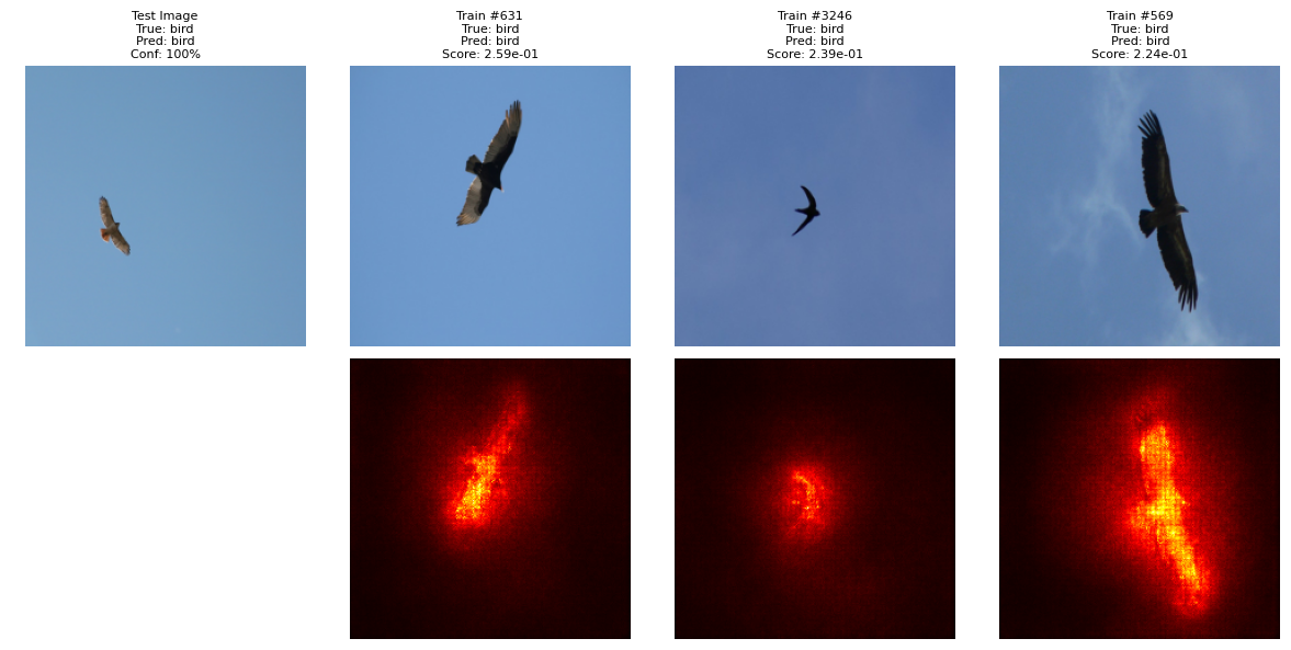
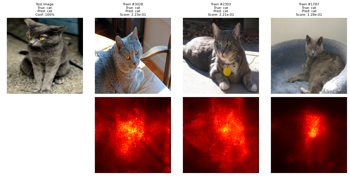
Figure 4: TFA saliencies (Equation 2) for the top-3 most influential training images per test image. Each panel (left to right): test image, influential training images, and their influence maps (smoothed using Equation 3).

4.2 Dependence on the test image

A key property of our method is that influence maps are test-specific: the same training image can produce different saliency patterns depending on the test instance, providing more specific explanations than using either feature-level attribution or training data attribution alone. To illustrate this effect, we consider the multi-label setting and select two test images from different classes (e.g., person and dog). We then compute pixelwise influence scores for the same training image containing both classes. As shown in Figure 5, the resulting heatmaps differ: the person region of the training image is most influential for the test image labeled “person,” whereas the dog region is most influential for the test image labeled “dog.”

 

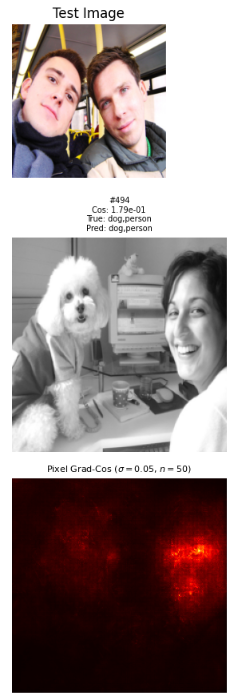
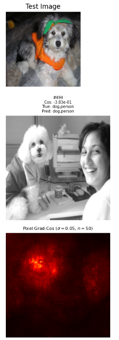
Figure 5: Two examples showing test-image dependence of pixelwise influence maps. In each example, the same training image yields different saliency patterns depending on the test image label. Left pair: dog vs person ; Right pair: cat vs person.

4.3 Quantitative evaluation

We quantitatively test whether pixelwise influence maps identify the training pixels that most affect a given test example. On CIFAR-10 (Krizhevsky, 2009), we train a lightweight CNN for 10 epochs (Adam, $\text{lr}=10^{-3}$, batch size $64$) on $90\%$ of the training set and keep the remaining $10\%$ as a holdout pool. We then randomly pick $50$ test images $x^{\text{test}}$ and, for each, select the $M{=}20$ most positively influential holdout images using Grad-Cos on parameter gradients. For each selected pair $(x^{\text{train}},x^{\text{test}})$, we compute a smoothed pixelwise influence map (SmoothGrad with Gaussian noise $\sigma{=}0.05$ of the normalized range, $n{=}30$ samples). We use an insertion intervention: we retain only the top-$k\%$ most influential pixels of $x^{\text{train}}$, replacing the others with the dataset mean. As a baseline, we retain a random $k\%$ of pixels. We then perform a single additional SGD step (no momentum, $\text{lr}_{\text{step}}{=}10^{-3}$) on the loss computed for the masked $x^{\text{train}}$ and measure the change in loss on $x^{\text{test}}$,

$$\Delta\mathcal{L}\;=\;\mathcal{L}_{\text{new}}(x^{\text{test}})-\mathcal{L}_{\text{old}}(x^{\text{test}}),$$

where more negative $\Delta\mathcal{L}$ indicates a more beneficial update for the test example. Each train–test pair is evaluated under both conditions (Top-$k$ vs. Random), and we report the paired difference $\Delta(T{-}R){=}\Delta\mathcal{L}_{\text{topk}}-\Delta\mathcal{L}_{\text{rand}}$ with normal-approximate $95\%$ confidence intervals (CI) over $1000$ pairs per $k$.

If the heatmaps correctly localize influential pixels, then inserting the Top-$k$ pixels should yield a strictly more negative test-loss change than inserting random pixels, i.e., $\Delta(T{-}R)<0$.

Results

Across a broad range of $k$, Top-$k$ insertion consistently yields more negative test-loss changes than the random control, with statistically significant paired gaps (Table 1). This quantitatively validates that the proposed TFA saliency maps obtained by combining grad-cos with Smoothgrad surface important training pixels associated to the prediction on a given test instance. As expected, the effect diminishes as $k$ increases (reduced selectivity) and vanishes at $k{=}100\%$ by construction.

$k$ (%)	$\mathbb{E}[\Delta\mathcal{L}_{\text{rand}}]$	$\mathbb{E}[\Delta\mathcal{L}_{\text{topk}}]$	$\mathbb{E}[\Delta(T{-}R)]\;\pm\;95\%\text{ CI}$
10	$-0.0829$	$-0.1560$	$-0.0730\;[\!-0.1163,\,-0.0298]$
20	$+0.0831$	$-0.0782$	$-0.1613\;[\!-0.2149,\,-0.1077]$
30	$+0.0739$	$-0.0422$	$-0.1161\;[\!-0.1644,\,-0.0678]$
40	$+0.0504$	$-0.0523$	$-0.1027\;[\!-0.1466,\,-0.0589]$
50	$-0.0086$	$-0.0661$	$-0.0576\;[\!-0.1002,\,-0.0150]$
60	$-0.0312$	$-0.0857$	$-0.0545\;[\!-0.0958,\,-0.0133]$
70	$-0.0786$	$-0.0995$	$-0.0208\;[\!-0.0572,\,+0.0155]$
100	$-0.2175$	$-0.2175$	$-0.0000\;[\!-0.0000,\,+0.0000]$

Table 1: Paired intervention results (CIFAR-10). Negative $\Delta(T{-}R)$ indicates that Top-$k$ TFA scores insertion improves $x^{\text{test}}$ loss more than a random $k\%$ insertion for the same train–test pair.

5 Use Cases

5.1 Explaining a wrong prediction

A common diagnostic task in model interpretability is to explain why a model makes an incorrect prediction. Our method is well-suited for this, as it identifies not only the training examples most responsible for a given test prediction, but also the specific regions within those training images that contribute to the error.

The practical pipeline is as follows: Given a classification task, suppose a test image is misclassified as class $B$ instead of its correct class $A$. We compute the Grad-Cos scores between the test image and all training images, then sort the training set by these scores. High scores correspond to helpful examples that support correct predictions, whereas low scores reveal the most harmful training instances; training on such an image for one additional step would be expected to increase the loss on the test image. In practice, these harmful examples often contain class $B$ in their labels.

To localize the regions in these harmful training images that drive the misclassification, we apply our TFA method. Figure 8 illustrates this process. The test image (a sheep misclassified as a dog) is most harmed by (1) an image of a dalmatian, which visually resembles the sheep, and (2) an image containing both a dog and a sheep, where the influence map shows the model relying on the dog region when predicting the test image.

figureb[floatrow]floatrowcapbesideposition=left,center,capbesidewidth=.29floatbesidecapbesidefloatfigurebesidecapbesidefigureb[floatrow]floatrowcapbesideposition=left,center,capbesidewidth=.29floatbesidecapbesidefloatfigurebesidecapbesidefigureb [floatrow]floatrowcapbesideposition=left,center,capbesidewidth=.29floatbesidecapbesidefloatfigurebesidecapbesidefigureb Figure 8: For a test image of a sheep misclassified as dog, the two most influential training images are (1) a dalmatian, and (2) an image containing both a dog and sheep. The influence maps show the model relies on the dog regions when predicting the test image.

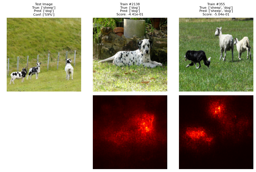
5.2 Detecting Spurious Correlations via Patch-Based Shortcuts

Spurious correlations refer to statistical associations in the training data that do not reflect meaningful or causal relationships, but rather arise due to dataset biases or artifacts. As a result, deep learning models can base their decisions on such shortcuts, for example by relying on background cues or artificial patterns, instead of learning to recognize the actual object of interest (Izmailov et al., 2022; Xiao et al., 2020). To reveal these hidden biases, it is useful not only to identify which training images most influence a model’s predictions, but also to localize the specific regions within those images that drive the decision. Motivated by this, we design a patch-based experiment to assess a model’s reliance on a synthetically constructed spurious feature. Specifically, we construct a binary classification task (sheep vs. cow) and introduce a colored patch (a red square in the bottom right corner) to training images containing sheep, while leaving the validation and test images unaltered. We fine-tune a pretrained ResNet-18 on this biased dataset. The model quickly learns to rely on the presence of the patch as a shortcut for identifying sheep. As a result, during evaluation, the model frequently misclassifies sheep in test images without the patch as cows.

As a comparison to what we would obtain using classical feature attribution, we then apply the off-the-shelf saliency method Grad-CAM (Selvaraju et al., 2017) to a misclassified test image. Grad-CAM primarily highlights the sheep itself, failing to reveal the true cause of the misclassification. This is expected, as the spurious patch is absent from the test image and therefore invisible to methods that only analyze test-time features. Detecting such correlations instead requires examining the training data through training data attribution methods. Using the gradient-cosine similarity, we find that the most influential training images are those containing sheep along with the patch. The corresponding pixelwise saliency maps confirm that the model’s predictions are driven largely by the presence of the patch rather than by the animal itself (Figure 9).

Additionally, in Appendix D.3, a quantitative analysis examining the impact of progressively increasing the proportion of images containing the spurious patch demonstrates that, as the model’s reliance on the patch intensifies – resulting in a decrease in classification accuracy for the sheep class – the TFA method correspondingly assigns greater importance to the patch pixels in the training images (Figure 15 in Appendix D.3).

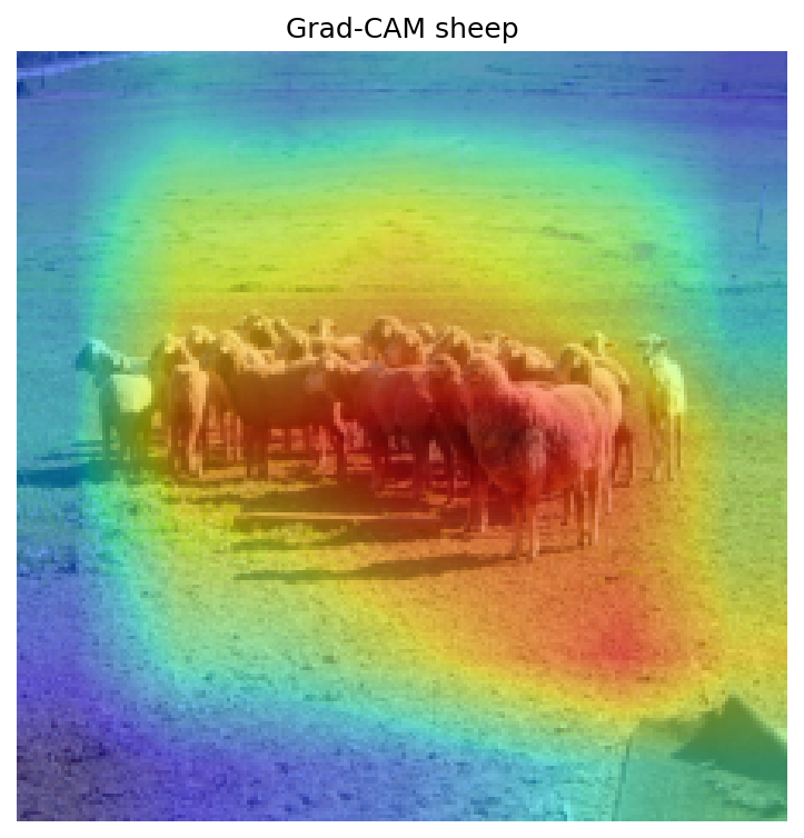
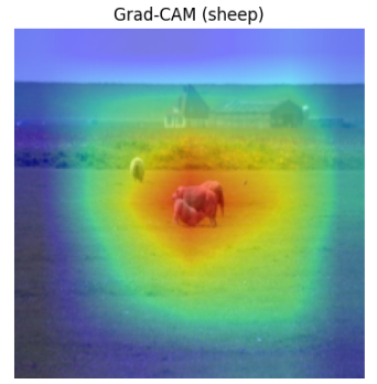
Figure 9: Left to right: (1) Test image of sheep, misclassified as cow; (2) Most influential training image (sheep); (3) Pixelwise influence map reveals the model heavily relies on the red patch for its prediction; (4) Grad-CAM map for the test image.

6 Conclusion

There exists an intrinsic tension between the growing complexity and opacity of deep learning models (always increasing number of parameters trained on ever-larger datasets), and the rising demand for accountability, reliability, and the ability to provide explanations for model decisions, particularly in cases of erroneous or biased outcomes. eXplainable AI (XAI) seeks to address this challenge by providing methodologies to interpret trained neural networks, effectively enabling a form of reverse engineering to elucidate their decision-making processes.

In this work, we proposed the training feature attribution (TFA) framework for vision models, designed to trace the patterns utilized during inference back to the specific training examples from which these patterns were learned. We empirically demonstrate that the proposed algorithm, which integrates the grad-cos TDA method with gradient-based FA, generates meaningful saliency maps on training examples. Furthermore, we present two practical use cases illustrating how TFA enhances our understanding of the internal mechanisms underlying model predictions.

Although this work concentrates on pixel-level attributions, the long-term objective is to extend the framework to encompass higher-level, human-interpretable concepts. Such an extension would provide a more abstract and semantically meaningful understanding of the model’s learned representations, as well as their origins within the training data.

Appendix A Analytic Toy Example for Training Feature Attribution

To illustrate the distinction between training data attribution (TDA) and training feature attribution (TFA), we consider a simple linear ridge regression model in $\mathbb{R}^{2}$. Because the model admits a closed-form solution, we can compute exact attributions and compare the two decompositions.

Setup

We define a linear predictor $f_{w}(x)=w^{\top}x$ with squared loss and $\ell_{2}$ regularization. The ground-truth rule is $y=x_{1}+x_{2}$, but the training data only reveal this partially: for $i=1,\ldots,n-1$ we provide samples on the $x_{1}$ axis,

$$x_{i}=(x_{i1},0),\quad y_{i}=x_{i1},$$

and a single informative point,

$$x_{n}=(0,c),\quad y_{n}=c,\qquad c\neq 0.$$

Let $X\in\mathbb{R}^{n\times 2}$ be the design matrix and $y\in\mathbb{R}^{n}$ the labels. We train with the ridge objective

$$L(w)=\tfrac{1}{2}\sum_{i=1}^{n}(w^{\top}x_{i}-y_{i})^{2}+\tfrac{\lambda}{2}\|w\|^{2},\qquad\lambda>0.$$

The closed-form solution is

$$w^{\star}=(X^{\top}X+\lambda I)^{-1}X^{\top}y=\Big(\tfrac{S_{11}}{S_{11}+\lambda},\;\tfrac{c^{2}}{c^{2}+\lambda}\Big),$$

where $S_{11}=\sum_{i\neq c}x_{i1}^{2}$. The Hessian of the objective is diagonal:

$$H=X^{\top}X+\lambda I=\mathrm{diag}(S_{11}+\lambda,\;c^{2}+\lambda).$$

We evaluate predictions at a test point $x_{\ast}=(0,t)$.

TDA (Representer Decomposition)

In ridge regression, the prediction can be written as

$$f_{w^{\star}}(x_{\ast})=\sum_{i=1}^{n}\alpha_{i}y_{i},\qquad\alpha_{i}=x_{\ast}^{\top}(X^{\top}X+\lambda I)^{-1}x_{i}.$$

For $x_{\ast}=(0,t)$ and $A=(X^{\top}X+\lambda I)^{-1}=\mathrm{diag}\!\left(\tfrac{1}{S_{11}+\lambda},\tfrac{1}{c^{2}+\lambda}\right)$, we obtain

$$\alpha_{i}=\frac{t}{c^{2}+\lambda}\,x_{i2}.$$

Thus $\alpha_{i}=0$ for $i\neq n$, and

$$\alpha_{n}y_{n}=\frac{tc^{2}}{c^{2}+\lambda}=f_{w^{\star}}(x_{\ast}).$$

All predictive mass is attributed to the single informative training example $z_{n}$.

Training Feature Attribution

We now refine the decomposition down to the level of individual features. For each training example $i$ and feature $k$, we define

$$\beta_{i,k}=\,x_{ik}\,(e_{k}^{\top}Ax_{\ast}),$$

where $e_{k}$ is the $k$-th standard basis vector, so that

$$f_{w^{\star}}(x_{\ast})=\sum_{i=1}^{n}y_{i}\sum_{k=1}^{2}\beta_{i,k}.$$

In our toy setup, $e_{1}^{\top}Ax_{\ast}=0$, hence $\beta_{i,1}=0$ for all $i$. Meanwhile,

$$e_{2}^{\top}Ax_{\ast}=\frac{t}{c^{2}+\lambda},\qquad\beta_{i,2}=\frac{t}{c^{2}+\lambda}\,x_{i2}.$$

Thus $\beta_{i,2}=0$ for all $i\neq n$, and

$$y_{n}\beta_{n,2}=\frac{tc^{2}}{c^{2}+\lambda}=f_{w^{\star}}(x_{\ast}).$$

Takeaway

Whereas TDA assigns all credit to the single informative training example $z_{n}$, TFA goes further and reveals that only the second feature of $z_{n}$ is responsible.

Appendix B From Influence Functions to Grad-Cos via RelatIF

As an alternative to grad-cos as choice of TDA method, the influence function (Hampel et al., 1986) from robust statistics quantifies the effect of an infinitesimal upweighting of a training example on a model’s output. It was adapted to modern deep learning models in (Koh & Liang, 2017) to estimate the effect of upweighting a single training example $z_{i}^{\text{train}}$ on the loss of a test example $z_{j}^{\text{test}}$:

$$I_{\mathrm{IF}}(i,j)=-\nabla_{\theta}\mathcal{L}(z_{j}^{\text{test}};\hat{\theta})^{\top}H_{\hat{\theta}}^{-1}\nabla_{\theta}\mathcal{L}(z_{i}^{\text{train}};\hat{\theta}),$$

where $H_{\hat{\theta}}$ is the Hessian of the empirical risk at the model parameters $\hat{\theta}$.

In practice, Koh and Liang note that when parameters $\tilde{\theta}$ are obtained via early stopping or in non-convex settings, $H_{\tilde{\theta}}$ may have negative eigenvalues. They address this by replacing $H_{\tilde{\theta}}$ with a damped version $H_{\tilde{\theta}}+\lambda I$, which corresponds to an $L_{2}$ regularization on the parameters and ensures positive-definiteness.

Our experiments with influence functions were not as satisfactory as expected (Figure 10), which is consistent with a previously reported limitation of influence functions (Barshan et al., 2020; Hanawa et al., 2021), in that the highest-scoring training points for a given test example are often high-loss or atypical samples (e.g., mislabeled data or outliers). Such points tend to appear in the top-$k$ lists for many different test examples, because maximizing $|I_{\mathrm{IF}}(i,j)|$ does not constrain how reweighting $z_{i}$ affects the model globally. To address this, Relative Influence Functions (RelatIF) were proposed, which normalize the influence by the magnitude of the parameter update induced by the training example, thereby emphasizing examples whose effect is more specific to the test point rather than globally dominant (Barshan et al., 2020).

Formally, RelatIF normalizes as follows:

$$S_{\mathrm{RelatIF},\lambda}(i,j)=-\frac{\nabla_{\theta}\mathcal{L}(z_{j}^{\text{test}})^{\top}(H_{\hat{\theta}}+\lambda I)^{-1}\nabla_{\theta}\mathcal{L}(z_{i}^{\text{train}})}{\|(H_{\hat{\theta}}+\lambda I)^{-1}\nabla_{\theta}\mathcal{L}(z_{i}^{\text{train}})\|}.$$

In the large-damping regime ($\lambda\gg\|H_{\hat{\theta}}\|$), the inverse can be approximated as:

$$(H_{\hat{\theta}}+\lambda I)^{-1}\approx\frac{1}{\lambda}I,$$

which simplifies the RelatIF score to:

$$S_{\mathrm{RelatIF},\lambda}(i,j)\approx-\frac{\nabla_{\theta}\mathcal{L}(z_{j}^{\text{test}})^{\top}\nabla_{\theta}\mathcal{L}(z_{i}^{\text{train}})}{\|\nabla_{\theta}\mathcal{L}(z_{i}^{\text{train}})\|}\cdot\frac{1}{\lambda}.$$

This is proportional to the gradient inner product between test and train examples, normalized by the train gradient norm. The gradient cosine similarity (Grad-Cos) (Charpiat et al., 2019) is defined as:

$$S_{\mathrm{GC}}(i,j)=\frac{\nabla_{\theta}\mathcal{L}(z_{j}^{\text{test}})^{\top}\nabla_{\theta}\mathcal{L}(z_{i}^{\text{train}})}{\|\nabla_{\theta}\mathcal{L}(z_{j}^{\text{test}})\|\;\|\nabla_{\theta}\mathcal{L}(z_{i}^{\text{train}})\|}.$$

For a fixed test point $j$, the term $\|\nabla_{\theta}\mathcal{L}(z_{j}^{\text{test}})\|$ is constant across all $i$, so large-$\lambda$ RelatIF and Grad-Cos produce similar rankings of training examples. Thus, Grad-Cos can be interpreted as the “no-curvature” limit of RelatIF, replacing the Hessian-inverse weighting by a simple directional similarity between gradients. While this interpretation is an approximation, it is reasonable in the large neural networks considered here, where the Hessian is expensive to compute, often ill-conditioned, and in practice dominated by its diagonal structure or noisy low-magnitude eigenvalues. In such settings, removing curvature information tends to yield more coherent attribution scores and explanations.

To illustrate this, Figure 10 compares the top 10 most influential training images for a given test image, as identified by Grad-Cos and by influence functions. While Grad-Cos selects visually similar training samples that align with intuitive, human-understandable explanations, influence functions often return atypical examples that appear to be outliers or high-loss points, offering less interpretable justifications.

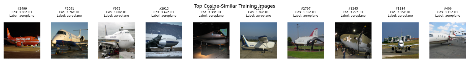
Figure 10: Top-10 most influential training images for a given test image, as identified by influence functions (top) and by Grad-Cos (bottom).

Appendix C Denoising saliency maps with SmoothGrad

Pixelwise influence maps, like other gradient-based saliency methods, are often dominated by noise and visually irrelevant fluctuations. While it remains uncertain whether this noise encodes real features of the learned model or simply results from the limitations of the attribution method, its presence can obscure meaningful interpretation. To obtain more robust and interpretable attributions, we combine our method with the SmoothGrad technique Smilkov et al. (2017): we perturb the training image with Gaussian noise, compute the attribution map for each noisy sample, and average the results. The resulting smoothed map is given by

$$\frac{1}{n}\sum_{1}^{n}\nabla_{x_{i}^{\text{train}}}S_{GC}\big(x_{i}^{\text{train}}+\mathcal{N}(0,\sigma^{2}I),z_{j}^{\text{test}}\big)$$ (3)

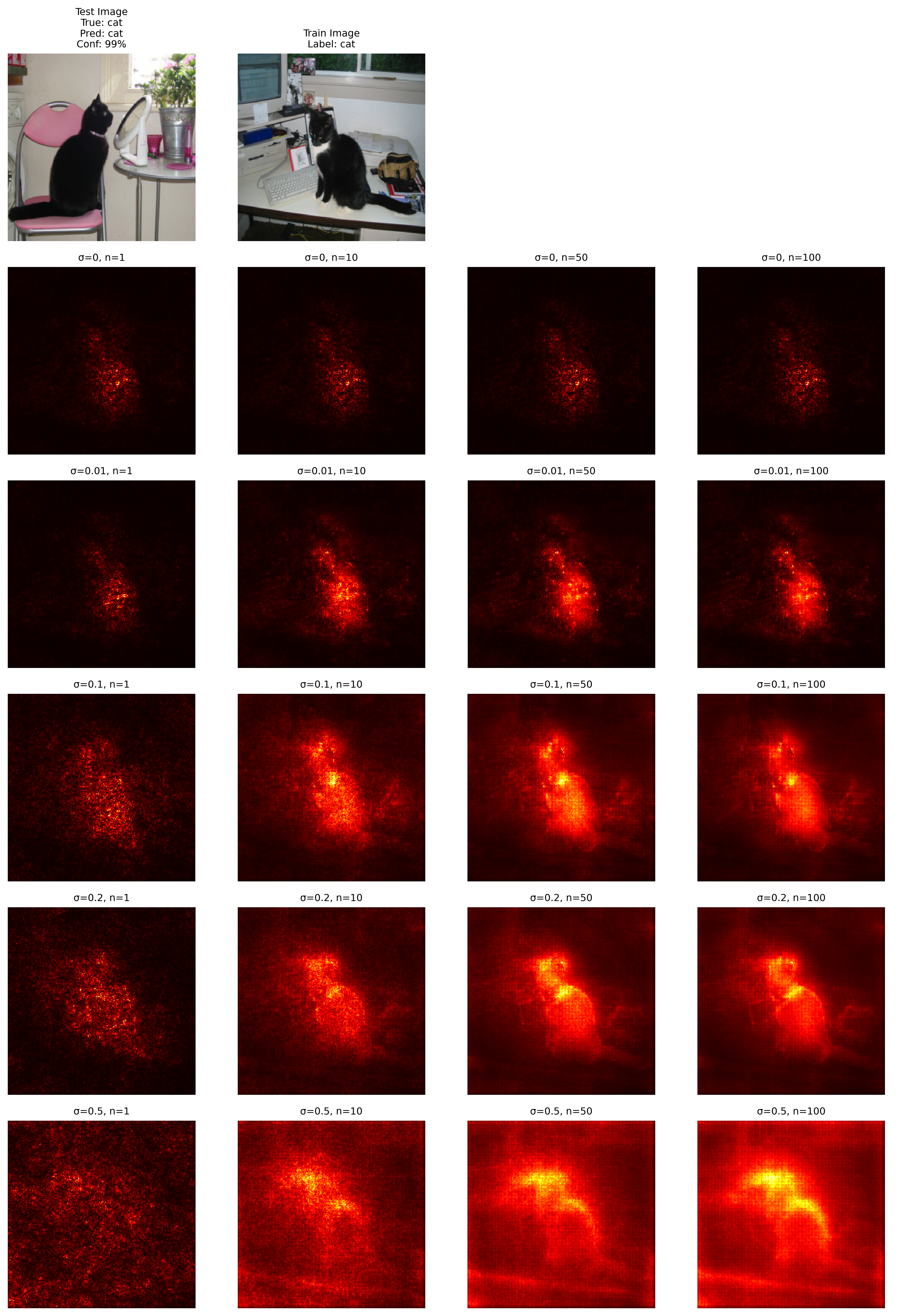
Figure 11: Effect of smoothing parameters on pixelwise influence maps. Each row corresponds to a different noise standard deviation $\sigma\in\{0,0.01,0.1,0.2,0.5\}$, and each column to a different number of noisy samples $n\in\{1,10,50,100\}$. Shown are the influence maps for a test image (left) predicted as cat and its most influential training image (right).

The rationale for this smoothing is that gradients in deep networks, especially those using ReLU activations, can exhibit sharp local fluctuations: small perturbations to the input can cause large, seemingly erratic changes in the gradient, even when the perturbed images appear indistinguishable to a human observer and are classified the same way by the model. These abrupt variations are often not meaningful, but rather artifacts of the model’s nonsmooth, piecewise-linear nature Smilkov et al. (2017). By adding Gaussian noise and averaging the resulting saliency maps, we approximate a local average of the gradient field, filtering out these unstable, high-frequency fluctuations while preserving the more robust and informative attributions. For a visualization of the effect of the noise standard deviation $\sigma$ and the number of samples $n$, see Figure 11. Based on these experiments, as well as the recommendations of (Smilkov et al., 2017), we set $\sigma$ to $[5\%,20\%]$ of the input dynamic range (for images, relative to the pixel intensity scale) and $n\approx 50$, which generally yields robust and interpretable maps.

Appendix D Additional experiments

D.1 Attribution to Layers

To analyze how different regions of an image at intermediate network layers influence predictions, we compute gradient-based attributions with respect to the activation map

$$h(x)\in\mathbb{R}^{C\times H\times W}$$

where $C$ is the number of feature channels, and $H\times W$ is the spatial resolution of the activation map at the chosen layer. For a test image $x^{\text{test}}$ and a training image $x^{\text{train}}_{i}$, we define:

$$\text{Saliency}(x^{\text{train}}_{i})\;=\;\left|\nabla_{h(x^{\text{train}}_{i})}\,\cos\!\left(\nabla_{h(x^{\text{test}})}\mathcal{L}(z_{i}^{\text{train}};\hat{\theta}),\;\nabla_{h(x^{\text{train}}_{i})}\mathcal{L}(z_{i}^{\text{train}};\hat{\theta})\right)\right|$$

where:

• $\nabla_{h(x)}$ denotes the gradient with respect to the activation map $h(x)$ at the chosen layer.

• The cosine similarity measures the alignment between the influence of test and training samples through that layer.

Averaging over channels yields a 2D spatial saliency map:

$$\text{Saliency2D}=\frac{1}{C}\sum_{c=1}^{C}\text{Saliency}_{c,:,:}$$

For example, for layer3 in ResNet-18, $(H,W)=(14,14)$. The resulting map is then upsampled (e.g., bilinear interpolation) to match the input resolution (e.g., $224\times 224$).

Figure 12 illustrates the outputs of this approach. As we move to deeper layers, the highlighted regions of the saliency maps appear smoother, which is expected since the maps are obtained by upsampling from progressively smaller activation maps. Nonetheless, the highlighted object remains consistent across layers, even when compared to the raw saliency map computed with respect to the training image. For the last convolutional layer (layer4), however, the focus on the object decreases and the most salient pixels extend over a larger portion of the image. This observation is consistent with the results reported in the Grad-CAM paper (Selvaraju et al., 2017) when experimenting with ResNets.

Figure 12: From left to right: test image, training image that includes a dog, pixelwise smoothed Grad-Cos saliency map ($\sigma{=}0.05$, $n{=}50$), and layerwise Grad-Cos saliency maps. Each layerwise map corresponds to the last convolutional layer in each residual block of the ResNet-18 architecture.

D.2 Varying models

To assess how architectural differences affect our pixelwise influence maps, we compare three backbones under the same training and preprocessing protocol: a ResNet-18 and a ResNet-50 (He et al., 2016), and a ViT-B/16 (Dosovitskiy et al., 2020) (all pretrained on ImageNet and fine-tuned on Pascal VOC 2012). For each test-train pair, we compute Smoothed Grad-Cos maps (Eq. 3) with $\sigma{=}0.1$ and $n{=}20$ noisy samples.

We observe (Figure 13) that the Vision Transformer consistently produces heatmaps with a visible patchwise structure. This effect stems from its architecture: ViT processes images as a sequence of non-overlapping patches (here $16{\times}16$ pixels), which are flattened and linearly projected into patch tokens. When computing gradients with respect to the input image, the backpropagation signal flows through this patch embedding step, so gradients are computed independently within each patch. As a result, the effective spatial resolution of the influence map is limited by the patch size, and channel-aggregated attributions often appear uniform within each patch.

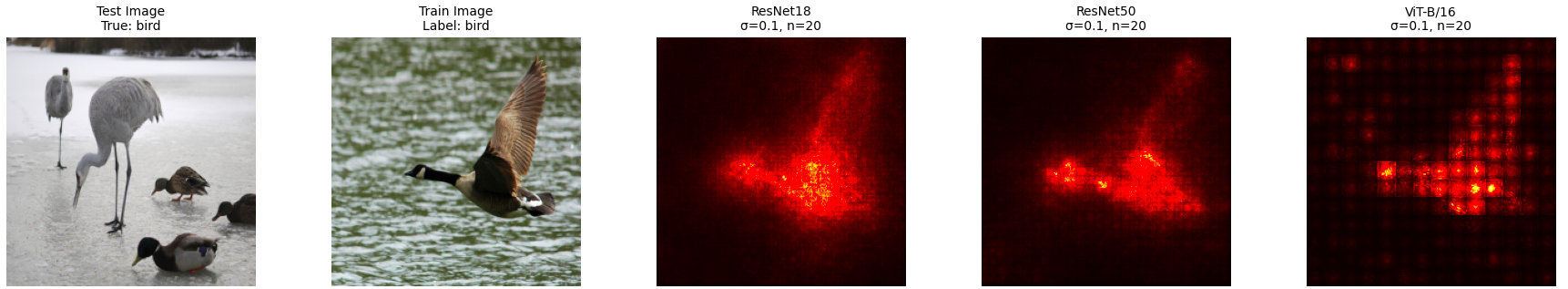
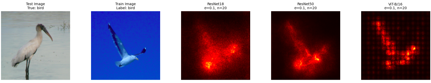
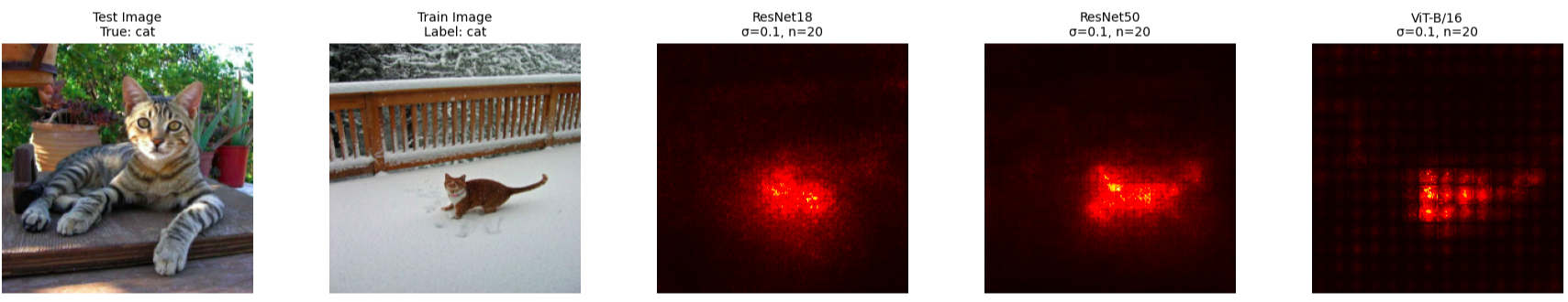
Figure 13: Influence comparison across backbones. Each row shows (from left to right): test image, a training image from the same class, and influence maps produced by ResNet-18, ResNet-50, and ViT-B/16 ($\sigma{=}0.1$, $n{=}20$).

Interestingly, we find that ResNet-50 is slightly less sensitive to noise compared to ResNet-18, likely due to its deeper architecture and larger receptive fields.

D.3 Quantitative Evaluation of Shortcut Detection on CIFAR-10

To quantitatively assess how effectively our method detects spurious correlations, and how strongly the model relies on them as a function of their prevalence in the training set, we design a controlled patch-based shortcut experiment.

We construct a subset of CIFAR-10 (Krizhevsky, 2009) containing three classes: dog, ship, and automobile. A square colored patch is inserted in the lower-right corner of a fixed proportion of the training images labeled as dog. This proportion (referred to as the patch fraction) denotes the percentage of dog training images that are patched, and we vary it across 17 values from 0% to 100%. For each patch fraction, we train the same lightweight CNN from scratch on the corresponding training set.

At evaluation time, to probe shortcut reliance, we also create a “patched-ship” test set by inserting the same patch into ship test images; all other test images remain unmodified. We then report: overall test accuracy, accuracy on unpatched dog images, and accuracy on patched ship images (to test whether the model associates the patch with the dog class).

As qualitative examples at four patch fractions (0%, 5%, 85%, 95%), see Figure 14.

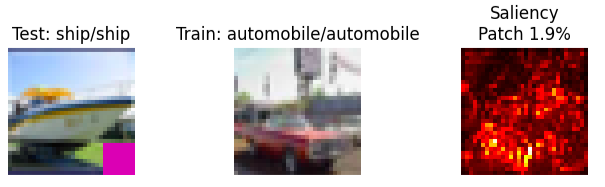
(a) Patch fraction 0%.

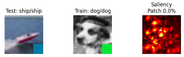
(b) Patch fraction 5%.

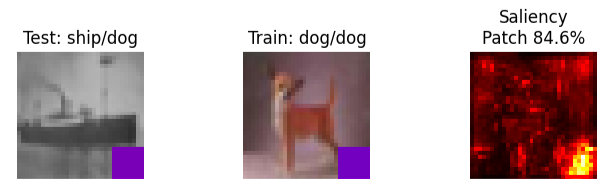
(c) Patch fraction 85%.

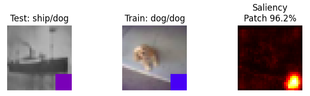
(d) Patch fraction 95%.

Figure 14: Qualitative triplets for the CIFAR-10 shortcut experiment at four patch prevalences. Each panel shows (left to right): the test image with true/predicted label, the most harmful training image, and the pixelwise influence map with the percentage of top-10% saliency inside the patch.

To verify whether our method localizes the shortcut, we apply training feature attribution to the patched-ship images. If the shortcut has been learned, these probes are increasingly misclassified as dog, and the influence maps should highlight the patch region. For each patch fraction, we sample five patched-ship test images, identify the ten most harmful training images (most oppositely aligned gradients), and compute pixelwise influence maps. We keep the top 10% most salient pixels and measure the proportion falling inside the patch (patch attribution fraction).

As shown in Figure 15a, as the fraction of dog training images with the patch increases, the accuracy on patched ship and unpatched dog images decreases, indicating that the model has adopted the patch as a shortcut. This effect is more pronounced for patched ships, which never co-occur with the patch during training and are thus quickly misclassified as dogs, whereas unpatched dogs remain recognizable until the patch prevalence becomes extreme. Consistently, Figure 15b shows a rising patch-attribution fraction, confirming that training feature attribution increasingly localizes to the patch region as its proportion grows.

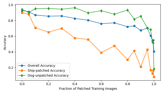
(a)

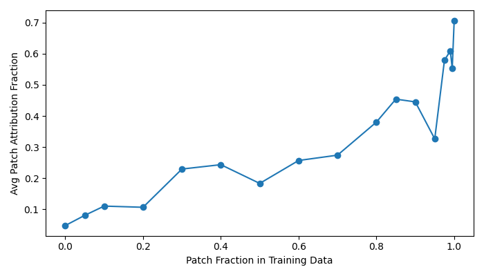
(b)

Figure 15: (a) Performance as the patch prevalence increases; (b) Localization of the shortcut via training feature attribution .

References

- Adebayo et al. (2018) Julius Adebayo, Justin Gilmer, Michael Muelly, Ian Goodfellow, Moritz Hardt, and Been Kim. Sanity checks for saliency maps. Advances in neural information processing systems, 31, 2018.
- Arjovsky et al. (2019) Martin Arjovsky, Léon Bottou, Ishaan Gulrajani, and David Lopez-Paz. Invariant risk minimization. arXiv preprint arXiv:1907.02893, 2019.
- Barshan et al. (2020) Elnaz Barshan, Marc-Etienne Brunet, and Gintare Karolina Dziugaite. Relatif: Identifying explanatory training samples via relative influence. In International Conference on Artificial Intelligence and Statistics, pp. 1899–1909. PMLR, 2020.
- Beery et al. (2018) Sara Beery, Grant Van Horn, and Pietro Perona. Recognition in terra incognita. In Proceedings of the European conference on computer vision (ECCV), pp. 456–473, 2018.
- Boggust et al. (2023) Angie Boggust, Harini Suresh, Hendrik Strobelt, John Guttag, and Arvind Satyanarayan. Saliency cards: a framework to characterize and compare saliency methods. In Proceedings of the 2023 ACM Conference on Fairness, Accountability, and Transparency, pp. 285–296, 2023.
- Byrne (2016) Ruth M.J. Byrne. Counterfactual thought. Annual Review of Psychology, 67:135–157, 2016. doi: 10.1146/annurev-psych-122414-033249. URL https://doi.org/10.1146/annurev-psych-122414-033249. First published online September 14, 2015.
- Charpiat et al. (2019) Guillaume Charpiat, Nicolas Girard, Loris Felardos, and Yuliya Tarabalka. Input similarity from the neural network perspective. Advances in Neural Information Processing Systems, 32, 2019.
- Chattopadhay et al. (2018) Aditya Chattopadhay, Anirban Sarkar, Prantik Howlader, and Vineeth N Balasubramanian. Grad-cam++: Generalized gradient-based visual explanations for deep convolutional networks. In 2018 IEEE winter conference on applications of computer vision (WACV), pp. 839–847. IEEE, 2018.
- Chen et al. (2019) Chaofan Chen, Oscar Li, Daniel Tao, Alina Barnett, Cynthia Rudin, and Jonathan K Su. This looks like that: deep learning for interpretable image recognition. Advances in neural information processing systems, 32, 2019.
- De Santis et al. (2024) Antonio De Santis, Riccardo Campi, Matteo Bianchi, and Marco Brambilla. Visual-tcav: concept-based attribution and saliency maps for post-hoc explainability in image classification. arXiv preprint arXiv:2411.05698, 2024.
- DeGrave et al. (2021) Alex J. DeGrave, Joseph D. Janizek, and Su-In Lee. Ai for radiographic covid-19 detection selects shortcuts over signal. Nature Machine Intelligence, 3:610–619, 2021. doi: 10.1038/s42256-021-00338-7. URL https://www.nature.com/articles/s42256-021-00338-7.
- Deng et al. (2009) Jia Deng, Wei Dong, Richard Socher, Li-Jia Li, Kai Li, and Li Fei-Fei. Imagenet: A large-scale hierarchical image database. In Proceedings of the IEEE Conference on Computer Vision and Pattern Recognition (CVPR), pp. 248–255, 2009.
- Devlin et al. (2019) Jacob Devlin, Ming-Wei Chang, Kenton Lee, and Kristina Toutanova. Bert: Pre-training of deep bidirectional transformers for language understanding. In Proceedings of NAACL-HLT 2019, pp. 4171–4186, 2019. URL https://aclanthology.org/N19-1423.pdf.
- Doshi-Velez & Kim (2017) Finale Doshi-Velez and Been Kim. Towards a rigorous science of interpretable machine learning. arXiv preprint arXiv:1702.08608, 2017.
- Dosovitskiy et al. (2020) Alexey Dosovitskiy, Lucas Beyer, Alexander Kolesnikov, Dirk Weissenborn, Xiaohua Zhai, Thomas Unterthiner, Mostafa Dehghani, Matthias Minderer, Georg Heigold, Sylvain Gelly, et al. An image is worth 16x16 words: Transformers for image recognition at scale. arXiv preprint arXiv:2010.11929, 2020.
- Everingham et al. (2015) Mark Everingham, S. M. Ali Eslami, Luc Van Gool, Christopher K. I. Williams, John Winn, and Andrew Zisserman. The pascal visual object classes challenge: A retrospective. International Journal of Computer Vision, 111(1):98–136, 2015. doi: 10.1007/s11263-014-0733-5.
- Fel et al. (2023) Thomas Fel, Agustin Picard, Louis Bethune, Thibaut Boissin, David Vigouroux, Julien Colin, Rémi Cadène, and Thomas Serre. Craft: Concept recursive activation factorization for explainability. In Proceedings of the IEEE/CVF Conference on Computer Vision and Pattern Recognition, pp. 2711–2721, 2023.
- Gentner (1983) Dedre Gentner. Structure-mapping: A theoretical framework for analogy. Cognitive Science, 7(2):155–170, 1983. doi: 10.1016/S0364-0213(83)80009-3. URL https://doi.org/10.1016/S0364-0213(83)80009-3.
- Ghorbani & Zou (2019) Amirata Ghorbani and James Zou. Data shapley: Equitable valuation of data for machine learning. In International conference on machine learning, pp. 2242–2251. PMLR, 2019.
- Grosse et al. (2023) Roger Grosse, Juhan Bae, Cem Anil, Nelson Elhage, Alex Tamkin, Amirhossein Tajdini, Benoit Steiner, Dustin Li, Esin Durmus, Ethan Perez, et al. Studying large language model generalization with influence functions. arXiv preprint arXiv:2308.03296, 2023.
- Hampel et al. (1986) Frank R. Hampel, Elvezio M. Ronchetti, Peter J. Rousseeuw, and Werner A. Stahel. Robust Statistics: The Approach Based on Influence Functions. Wiley, New York, 1986. ISBN 9780471735779. doi: 10.1002/9781118186435.
- Han et al. (2020) Xiaochuang Han, Byron C. Wallace, and Yulia Tsvetkov. Explaining Black Box Predictions and Unveiling Data Artifacts through Influence Functions, May 2020. URL http://arxiv.org/abs/2005.06676. arXiv:2005.06676 [cs].
- Hanawa et al. (2021) Kazuaki Hanawa, Sho Yokoi, Satoshi Hara, and Kentaro Inui. Evaluation of similarity-based explanations. In International Conference on Learning Representations, 2021. URL https://openreview.net/forum?id=9uvhpyQwzM_.
- He et al. (2016) Kaiming He, Xiangyu Zhang, Shaoqing Ren, and Jian Sun. Deep residual learning for image recognition. In Proceedings of the IEEE Conference on Computer Vision and Pattern Recognition (CVPR), pp. 770–778, 2016.
- Izmailov et al. (2022) Pavel Izmailov, Polina Kirichenko, Nate Gruver, and Andrew G Wilson. On feature learning in the presence of spurious correlations. Advances in Neural Information Processing Systems, 35:38516–38532, 2022.
- Kim et al. (2016) Been Kim, Rajiv Khanna, and Oluwasanmi O Koyejo. Examples are not enough, learn to criticize! criticism for interpretability. Advances in neural information processing systems, 29, 2016.
- Kim et al. (2018) Been Kim, Martin Wattenberg, Justin Gilmer, Carrie Cai, James Wexler, Fernanda Viegas, et al. Interpretability beyond feature attribution: Quantitative testing with concept activation vectors (tcav). In International conference on machine learning, pp. 2668–2677. PMLR, 2018.
- Kingma & Ba (2015) Diederik P. Kingma and Jimmy Ba. Adam: A method for stochastic optimization. In International Conference on Learning Representations (ICLR), 2015.
- Koh & Liang (2017) Pang Wei Koh and Percy Liang. Understanding black-box predictions via influence functions. In International conference on machine learning, pp. 1885–1894. PMLR, 2017.
- Krizhevsky (2009) Alex Krizhevsky. Learning multiple layers of features from tiny images. Technical report, University of Toronto, 2009.
- Lipton (2018) Zachary C Lipton. The mythos of model interpretability: In machine learning, the concept of interpretability is both important and slippery. Queue, 16(3):31–57, 2018.
- Lundberg & Lee (2017) Scott M Lundberg and Su-In Lee. A unified approach to interpreting model predictions. Advances in neural information processing systems, 30, 2017.
- Miller (2019) Tim Miller. Explanation in artificial intelligence: Insights from the social sciences. Artificial intelligence, 267:1–38, 2019.
- Pezeshkpour et al. (2021) Pouya Pezeshkpour, Sarthak Jain, Sameer Singh, and Byron C Wallace. Combining feature and instance attribution to detect artifacts. arXiv preprint arXiv:2107.00323, 2021.
- Poché et al. (2023) Antonin Poché, Lucas Hervier, and Mohamed-Chafik Bakkay. Natural Example-Based Explainability: a Survey. In World Conference on eXplainable Artificial Intelligence, Lisbon, Portugal, July 2023. URL https://hal.science/hal-04117520.
- Pruthi et al. (2020) Garima Pruthi, Frederick Liu, Satyen Kale, and Mukund Sundararajan. Estimating training data influence by tracing gradient descent. Advances in Neural Information Processing Systems, 33:19920–19930, 2020.
- Radford et al. (2021) Alec Radford, Jong Wook Kim, Chris Hallacy, Aditya Ramesh, Gabriel Goh, Sandhini Agarwal, Girish Sastry, Amanda Askell, Pamela Mishkin, Jack Clark, Gretchen Krueger, and Ilya Sutskever. Learning transferable visual models from natural language supervision. In Proceedings of the 38th International Conference on Machine Learning, volume 139 of Proceedings of Machine Learning Research, pp. 8748–8763. PMLR, 2021. URL https://proceedings.mlr.press/v139/radford21a.html.
- Ribeiro et al. (2016) Marco Tulio Ribeiro, Sameer Singh, and Carlos Guestrin. ” why should i trust you?” explaining the predictions of any classifier. In Proceedings of the 22nd ACM SIGKDD international conference on knowledge discovery and data mining, pp. 1135–1144, 2016.
- Rudin (2019) Cynthia Rudin. Stop explaining black box machine learning models for high stakes decisions and use interpretable models instead. Nature machine intelligence, 1(5):206–215, 2019.
- Selvaraju et al. (2017) Ramprasaath R Selvaraju, Michael Cogswell, Abhishek Das, Ramakrishna Vedantam, Devi Parikh, and Dhruv Batra. Grad-cam: Visual explanations from deep networks via gradient-based localization. In Proceedings of the IEEE international conference on computer vision, pp. 618–626, 2017.
- Simonyan et al. (2013) Karen Simonyan, Andrea Vedaldi, and Andrew Zisserman. Deep inside convolutional networks: Visualising image classification models and saliency maps. arXiv preprint arXiv:1312.6034, 2013.
- Smilkov et al. (2017) Daniel Smilkov, Nikhil Thorat, Been Kim, Fernanda Viégas, and Martin Wattenberg. Smoothgrad: removing noise by adding noise. arXiv preprint arXiv:1706.03825, 2017.
- Sundararajan et al. (2017) Mukund Sundararajan, Ankur Taly, and Qiqi Yan. Axiomatic attribution for deep networks. In International conference on machine learning, pp. 3319–3328. PMLR, 2017.
- Wickramasinghe et al. (2020) Chathurika S. Wickramasinghe, Daniel L. Marino, Javier Grandio, and Milos Manic. Trustworthy ai development guidelines for human system interaction. In 2020 13th International Conference on Human System Interaction (HSI), pp. 130–136, 2020.
- Xiao et al. (2020) Kai Xiao, Logan Engstrom, Andrew Ilyas, and Aleksander Madry. Noise or signal: The role of image backgrounds in object recognition. arXiv preprint arXiv:2006.09994, 2020.
- Zeiler & Fergus (2014) Matthew D Zeiler and Rob Fergus. Visualizing and understanding convolutional networks. In European conference on computer vision, pp. 818–833. Springer, 2014.