Riemann-Silberstein geometric phase for high-dimensional light manipulation

Abstract

Geometric phases provide a powerful mechanism for light manipulation. In particular, the Pancharatnam-Berry (PB) phase has enabled optical metasurfaces with broad applications. However, the PB phase is based on polarization evolution in a two-dimensional space, which fails to account for other polarization degrees of freedom. Here, we generalize the concept of geometric phase to a four-dimensional (4D) Riemann-Silberstein (RS) space that characterizes the complete electromagnetic polarization, including electric, magnetic, and hybrid polarizations. We show that the 4D polarization evolution in the RS space can give rise to a new geometric phase—the RS phase—in addition to the PB phase. The PB phase depends on optical spin and usually manifests in circularly polarized light, whereas the RS phase depends on optical linear momentum and can manifest in arbitrarily polarized light. Their synergy provides a unified geometric framework for light propagation at interfaces and enables unprecedented high-dimensional light control. As a proof of principle, we propose and demonstrate RS metasurfaces capable of multiplexed wavefront shaping, which can reconfigure up to twelve distinct outputs via switching incident 4D polarization. Our work uncovers a new class of optical geometric phases, with promising applications in high-capacity optical communication, parallel information processing, and multifunctional nanophotonic design.

Introduction

Geometric phases emerge from state evolution in parameter space and provide a unified framework for understanding fundamental phenomena in quantum and classical physics [1, 2, 3, 4]. These phases have been extensively studied in diverse physical systems, including quantum particles [2, 5, 6, 7], condensed matter [8, 9], and classical wave systems [10, 11, 12, 13]. In optics, geometric phases can give rise to intriguing phenomena such as spin-orbit interactions [14] and photonic topological states [15, 16, 17, 18], providing profound insights into the geometric and topological properties of optical fields [19, 20, 21, 22] and enabling novel mechanisms for light manipulation [23, 24, 25, 26, 27, 28].

The optical PB phase has recently attracted significant attention for its crucial role in wavefront manipulation by metasurfaces [29, 30, 31, 32, 33, 34, 35, 36]. This phase arises from SU(2) polarization evolution on the Poincaré sphere [37, 38], which is a 2D space describing the polarization of a two-component vector field. However, light is an electromagnetic wave comprising an electric field $\mathbf{E}$ and a magnetic field $\mathbf{H}$, which form a bispinor in the Dirac-like framework [39, 40]. For monochromatic waves, both $\mathbf{E}$ and $\mathbf{H}$ are two-component vector fields within the local frame defined by their polarization ellipses [19, 41], and their polarizations can be different. Consequently, the complete polarization state of a monochromatic electromagnetic wave resides in a 4D Hilbert space (i.e., direct sum of electric and magnetic polarization spaces), termed RS space in this paper, which simultaneously characterizes electric, magnetic, and hybrid electric-magnetic polarizations. The SU(4) evolution of the 4D complete polarization can generate nontrivial geometric phases beyond the conventional PB phase, which has thus far remained elusive. These geometric phases are essential to understanding the complete vector properties of light and making full use of its degrees of freedom.

In this work, we extend the polarization space from 2D to 4D and investigate the geometric phase emerging from SU(4) evolution of the complete electromagnetic polarization. We identify a new class of geometric phase—the RS phase, which is governed by the hybrid electric-magnetic polarization, in contrast to the conventional PB phase associated with the individual electric (magnetic) polarization. The complementary nature of the RS and PB phases enables a geometric description of the phase shifts induced by light transmission and reflection at interfaces. Leveraging this dual-phase mechanism, we propose and demonstrate RS metasurfaces that can achieve high-dimensional wavefront manipulation, generating up to twelve distinct output wavefronts under the normal incidence of a plane wave with switchable 4D polarization.

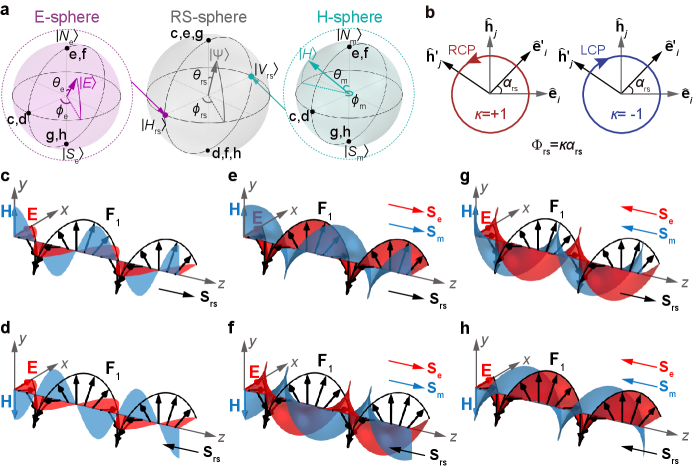
Figure 1: Complete 4D polarization of electromagnetic fields. (a) Poincaré hypersphere representation of 4D electromagnetic polarization, where the points “c-h” represent the polarizations of the plane waves in the panels (c-h), respectively. (b) RS geometric phase induced by the rotation of the local constitutive frame. Electric field (in red), magnetic field (in blue), and hybrid RS field (in black) of (c) $+z$-propagating linearly polarized plane wave, (d) $-z$-propagating linearly polarized plane wave, (e) $+z$-propagating RCP plane wave, (f) $-z$-propagating RCP plane wave, (g) $+z$-propagating LCP plane wave, and (h) $-z$-propagating LCP plane wave. The electric spin density $\mathbf{S_{\mathrm{e}}}$, magnetic spin density $\mathbf{S_{\mathrm{m}}}$, and RS spin density $\mathbf{S_{\mathrm{rs}}}$ are denoted by the red, blue, and black arrows, respectively.

Results

4D polarization with Poincaré hypersphere representation

A monochromatic electromagnetic field in three-dimensional space can be described by the wave field $\bm{\Psi}=\mathbf{E}+\mathrm{i}\mathbf{H}$, where $\mathbf{E}(\mathbf{r},t)=E_{i}(\mathbf{r},t)\hat{\mathbf{e}}_{i}+E_{j}(\mathbf{r},t)\hat{\mathbf{e}}_{j}$ is the complex electric field in the local frame with bases $\left(\hat{\mathbf{e}}_{i},\hat{\mathbf{e}}_{j}\right)$, and $\mathbf{H}(\mathbf{r},t)=H_{i}(\mathbf{r},t)\hat{\mathbf{h}}_{i}+H_{j}(\mathbf{r},t)\hat{\mathbf{h}}_{j}$ is the complex magnetic field in the local frame with bases $(\hat{\mathbf{h}}_{i},\hat{\mathbf{h}}_{j})$. Gaussian units are used in the formulations. We note that $\mathbf{E}$ and $\mathbf{H}$ are in orthogonal spaces, i.e., they do not mix in the wave field $\bm{\Psi}$. The wave field $\bm{\Psi}$ exhibits both internal polarizations (i.e., the polarizations of individual $\mathbf{E}$ and $\mathbf{H}$ fields) and external polarization (i.e., the hybrid $\mathbf{E}$-$\mathbf{H}$ polarization), characterized by the 4D polarization state $|\Psi\rangle$ residing in the 4D RS space. This 4D polarization can be described by a Poincaré hypersphere [42, 43], as illustrated in Fig. 1a, which comprises three nested Poincaré spheres: E-sphere characterizing the $\mathbf{E}$ field polarization, H-sphere characterizing the $\mathbf{H}$ field polarization, and RS-sphere characterizing the hybrid $\mathbf{E}$-$\mathbf{H}$ polarization. The E-sphere has the north pole state $\left|N_{\mathrm{e}}\right\rangle$ corresponding to right-handed circularly-polarized (RCP) electric field and the south pole state $\left|S_{\mathrm{e}}\right\rangle$ corresponding to left-handed circularly-polarized (LCP) electric field; The H-sphere has the north pole state $\left|N_{\mathrm{m}}\right\rangle$ corresponding to RCP magnetic field and the south pole state $\left|S_{\mathrm{m}}\right\rangle$ corresponding to the LCP magnetic field. Any other point on the E-sphere or H-sphere denotes a $\mathrm{SU}(2)$ superposition state parameterized by the polar angle $\theta_{\mathrm{e},\mathrm{m}}$ and azimuthal angle $\phi_{\mathrm{e},\mathrm{m}}$. Notably, the RS-sphere characterizes the relationship between E-sphere and H-sphere with $\theta_{\mathrm{rs}}$ and $\phi_{\mathrm{rs}}$; its horizontal basis state $\left|H_{\mathrm{rs}}\right\rangle$ corresponds to an arbitrary state on the E-sphere; its vertical basis state $\left|V_{\mathrm{rs}}\right\rangle$ corresponds to an arbitrary state on the H-sphere. Any other point on the RS-sphere denotes a $\operatorname{SU}(4)$ superposition state $|\Psi\rangle$ (see Methods).

In the following, we will focus on paraxial waves involving transverse electric and magnetic fields that are mutually perpendicular. In such cases, $\mathbf{E}$ and $\mathbf{H}$ exhibit the same polarization, and $\bm{\Psi}$ can be decomposed into a pair of orthogonal RS vectors: $\bm{\Psi}=\mathbf{F}_{1}+\mathbf{F}_{2}$, where $\mathbf{F}_{1}(\mathbf{r},t)=E_{i}(\mathbf{r},t)\hat{\mathbf{e}}_{i}+\mathrm{i}H_{j}(\mathbf{r},t)\hat{\mathbf{h}}_{j}$ and $\mathbf{F}_{2}(\mathbf{r},t)=E_{j}(\mathbf{r},t)\hat{\mathbf{e}}_{j}+\mathrm{i}H_{i}(\mathbf{r},t)\hat{\mathbf{h}}_{i}$. Consequently, the hybrid $\mathbf{E}$-$\mathbf{H}$ polarization reduces to the polarizations of the RS fields $\mathbf{F}_{1}$ and $\mathbf{F}_{2}$. We note that the RS vectors $\mathbf{F}_{1}$ and $\mathbf{F}_{2}$ are composed of complex electric and magnetic fields, which are different from the conventional RS vector comprising real electric and magnetic fields [44, 45, 46, 47, 48].

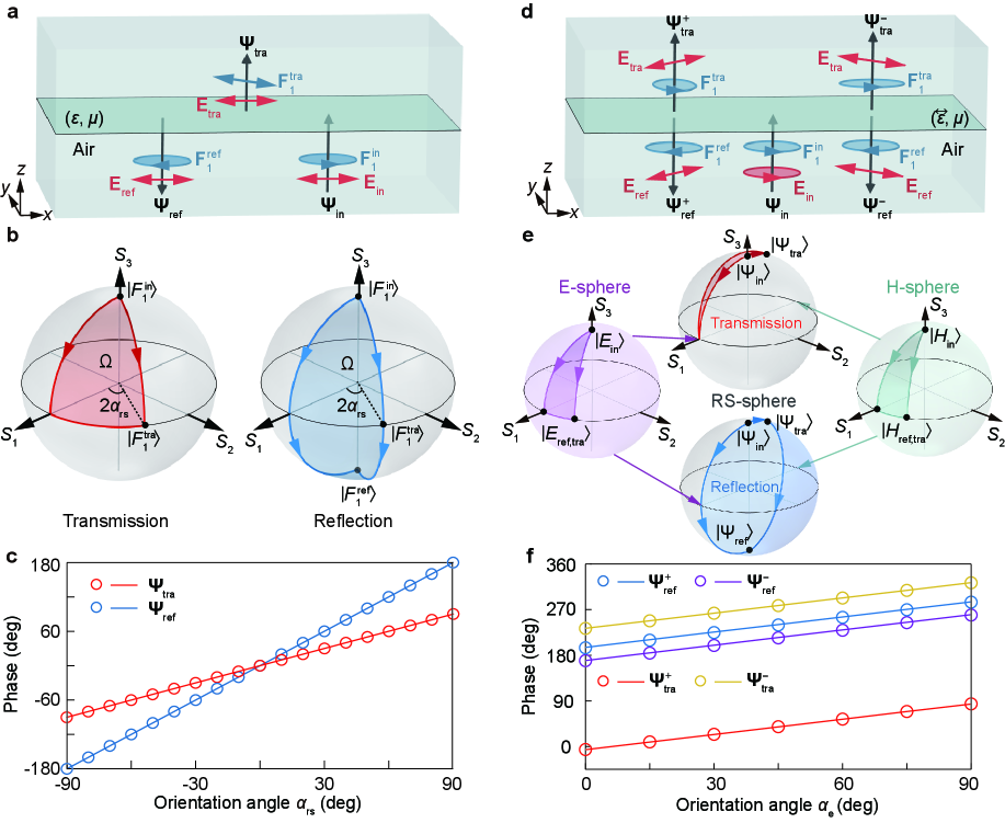
Figure 2: RS geometric phase at interfaces. (a) A plane wave with linearly polarized electric and magnetic fields impinges on an interface of isotropic media, where the RS polarization (blue arrows) undergoes evolutions but electric polarization (red arrows) remains unchanged. (b) Representation of the RS polarization evolution on the RS-sphere for the wave transmission and reflection. We choose the point on ${S}_{1}$ axis as the reference polarization. (c) Transmission and reflection phases for different orientation angles of the transmitted RS polarization. The circles denote the RS geometric phase. (d) A plane wave with circularly polarized electric and magnetic fields impinges on an interface of anisotropic media, where both the electric polarization (red arrows) and the RS polarization (blue arrows) undergo evolutions. (e) Representation of the 4D polarization evolution on the Poincaré hypersphere for the wave transmission and reflection. (f) Transmission and reflection phases for different orientation angle of the electric polarization. The circles denote the total geometric phase.

We use electromagnetic plane waves as an example to illustrate the 4D polarization and its representation on the Poincaré hypersphere. We first consider a plane wave with linearly polarized electric and magnetic fields: $\bm{\Psi}=(\hat{\mathbf{e}}_{x}+\mathrm{i}\kappa\hat{\mathbf{h}}_{y})Ee^{\mathrm{i}\kappa k_{0}z-\mathrm{i}\omega t}$, where $\kappa=\pm 1$ denotes the sign of the propagation direction relative to $+z$ axis. Figures 1c and 1d show the instantaneous $\mathbf{E}$, $\mathbf{H}$, and $\mathbf{F}_{1}$ fields for $\kappa=1$ and $\kappa=-1$, respectively. The polarizations of $\mathbf{E}$ and $\mathbf{H}$ fields are represented by points “c” and “d” on the E-sphere and H-sphere in Fig. 1a. The RS field $\mathbf{F}_{1}$ is RCP for $\kappa=1$ and LCP for $\kappa=-1$, which are represented by points “c” and “d” on the RS-sphere in Fig. 1a. Naturally, we can introduce an RS spin density $\mathbf{S}_{\mathrm{rs}}=\frac{1}{16\pi\omega}\operatorname{Im}\left[\mathbf{F}_{1}^{*}\times\mathbf{F}_{1}\right]=\frac{1}{\omega c}\mathbf{P}$, where $\mathbf{P}=\frac{c}{8\pi}\operatorname{Re}\left[\mathbf{E}^{*}\times\mathbf{H}\right]$ is the time-averaged Poynting vector. This RS spin characterizes the “chirality” of power flow, and its “handedness” is defined by $\kappa=\pm 1$.

We further consider a plane wave with circularly polarized electric and magnetic fields: $\bm{\Psi}=[\left(\hat{\mathbf{e}}_{x}+\mathrm{i}\sigma_{\mathrm{e}}\hat{\mathbf{e}}_{y}\right)+\mathrm{i}\kappa(\hat{\mathbf{h}}_{y}-\mathrm{i}\sigma_{\mathrm{m}}\hat{\mathbf{h}}_{x})]Ee^{\mathrm{i}\kappa k_{0}z-\mathrm{i}\omega t}$, where $\sigma_{\mathrm{e}}=\pm 1$ denotes the electric spin, $\sigma_{\mathrm{m}}=\pm 1$ denotes the magnetic spin, and $\kappa=\pm 1$ denotes the RS spin. Note that $\sigma_{\mathrm{e}}=\sigma_{\mathrm{m}}$ for plane waves. The total spin density can be expressed as $\mathbf{S}=\frac{1}{16\pi\omega}\operatorname{Im}\left[\bm{\Psi}^{*}\times\bm{\Psi}\right]=\mathbf{S}_{\mathrm{e}}+\mathbf{S}_{\mathrm{m}}+\mathbf{S}_{\mathrm{rs}}$, where $\mathbf{S}_{\mathrm{e}}=\frac{1}{16\pi\omega}\operatorname{Im}\left[\mathbf{E}^{*}\times\mathbf{E}\right]$ is the electric spin density, $\mathbf{S}_{\mathrm{m}}=\frac{1}{16\pi\omega}\operatorname{Im}\left[\mathbf{H}^{*}\times\mathbf{H}\right]$ is the magnetic spin density, and $\mathbf{S}_{\mathrm{rs}}=\frac{1}{16\pi\omega}\operatorname{Im}\left[\mathbf{F}_{1}^{*}\times\mathbf{F}_{1}\right]+\frac{1}{16\pi\omega}\operatorname{Im}\left[\mathbf{F}_{2}^{*}\times\mathbf{F}_{2}\right]=\frac{1}{\omega c}\mathbf{P}$ is the RS spin density. Notably, the sum of $\mathbf{S}_{\mathrm{e}}$ and $\mathbf{S}_{\mathrm{m}}$ corresponds to the conventional optical spin density that has been extensively studied in recent years [14, 49, 50, 51, 52, 53, 54], while the RS spin density $\mathbf{S}_{\mathrm{rs}}$ has been largely overlooked [48, 55]. Figure 1e-h shows the instantaneous $\mathbf{E}$, $\mathbf{H}$, $\mathbf{F}_{1}$, and spin directions for the plane waves with $\left(\sigma_{\mathrm{e}},\sigma_{\mathrm{m}},\kappa\right)=(+1,+1,+1),(+1,+1,-1),(-1,-1,+1)$, and $(-1,-1,-1)$, respectively. Their 4D polarizations are represented on the Poincaré hypersphere in Fig. 1a as the points “e”, “f”, “g”, and “h”, respectively.

The evolution of 4D polarization state $|\Psi\rangle$ simultaneously traces out paths on the E-sphere, H-sphere, and RS-sphere. The electric (magnetic) polarization evolution can generate the PB phase $\Phi_{\mathrm{pb}}$, which is proportional to the solid angle subtended by the area enclosed by the evolution path on E-sphere (H-sphere) [1]. Notably, the electric and magnetic polarization evolutions are intrinsically linked through the Maxwell equations. For the considered paraxial waves, the electric and magnetic polarization evolutions trace the same path and contribute to the same PB phase. Additionally, a new type of geometric phase can arise from the evolution of RS polarization (i.e., the polarization of $\mathbf{F}_{1,2}$). This geometric phase, termed RS phase and denoted as $\Phi_{\mathrm{rs}}$, is proportional to the solid angle subtended by the area enclosed by the evolution path on the RS-sphere (Supplementary Note II). Importantly, $\Phi_{\mathrm{rs}}$ is independent of $\Phi_{\mathrm{pb}}$ because $\Phi_{\mathrm{pb}}$ manifests in the basis states $\left|H_{\mathrm{rs}}\right\rangle$ and $\left|V_{\mathrm{rs}}\right\rangle$. Therefore, the total geometric phase due to 4D polarization evolution is $\Phi_{\mathrm{tot}}=\Phi_{\mathrm{pb}}+\Phi_{\mathrm{rs}}$.

The PB phase can be attributed to the coupling between electric (magnetic) spin and rotation of local coordinate frame, where the frame rotation induces a phase variation of the circularly polarized electric (magnetic) field [14]. Similarly, the RS phase can be attributed to the coupling between RS spin and rotation of local constitutive frame $(\hat{\mathbf{e}}_{i},\hat{\mathbf{h}}_{j})[\text{or }(\hat{\mathbf{e}}_{j},\hat{\mathbf{h}}_{i})]$, as shown in Fig. 1b. A rotation of the constitutive frame by angle $\alpha_{\mathrm{rs}}$ leads to the transformation of the circularly polarized RS vector: $\mathbf{F}_{1,2}\rightarrow\mathrm{e}^{\mathrm{i}\kappa\alpha_{\mathrm{rs}}}\mathbf{F}_{1,2}$. The phase $\kappa\alpha_{\mathrm{rs}}$ corresponds to the RS geometric phase, which is proportional to the RS spin $\kappa$ and the rotation angle $\alpha_{\mathrm{rs}}$ of the local constitutive frame.

RS geometric phase at interfaces

The RS phase can emerge in light transmission and reflection at an interface due to the evolution of 4D polarization. Such polarization evolution is determined by the eigen properties of the media separated by the interface. As shown in Fig. 2a, we consider that a plane wave propagates along $+z$ direction and normally impinges on the surface of an isotropic medium with permittivity $\varepsilon$ and permeability $\mu$. The incident electric (magnetic) field is linearly polarized in $x$ ($y$) direction. We denote the RS polarization states of the incident, reflected, and transmitted waves as $\left|F_{1}^{\text{in}}\right\rangle,\left|F_{1}^{\text{ref}}\right\rangle$, and $\left|F_{1}^{\text{tra}}\right\rangle$, respectively. The transmission involves the polarization evolution $\left|F_{1}^{\text{in}}\right\rangle\rightarrow\left|F_{1}^{\text{tra}}\right\rangle$, while the reflection involves the polarization evolution $\left|F_{1}^{\text{in}}\right\rangle\rightarrow\left|F_{1}^{\text{tra}}\right\rangle\rightarrow\left|F_{1}^{\text{ref}}\right\rangle$. These RS polarization evolutions induce the RS phases $\Phi_{\mathrm{rs}}^{\text{tra}}$ and $\Phi_{\mathrm{rs}}^{\mathrm{ref}}$, which manifest in the transmitted and reflected waves, respectively. As an example, we assume the medium is a lossless metal. In this case, $\left|F_{1}^{\mathrm{in}}\right\rangle=\frac{1}{\sqrt{2}}(\hat{\mathbf{e}}_{x}+\mathrm{i}\hat{\mathbf{h}}_{y}),\left|F_{1}^{\mathrm{ref}}\right\rangle=\frac{1}{\sqrt{2}}(\hat{\mathbf{e}}_{x}-\mathrm{i}\hat{\mathbf{h}}_{y})$, and $\left|F_{1}^{\text{tra}}\right\rangle=\frac{\sqrt{\left|{\mu}\right|}}{\sqrt{\left|{\mu}\right|+\left|{\varepsilon}\right|}}(\hat{\mathbf{e}}_{x}+\frac{\mathrm{i\sqrt{\varepsilon}}}{\sqrt{\mu}}\hat{\mathbf{h}}_{y})$. Notably, $\left|F_{1}^{\text{tra}}\right\rangle$ is linearly polarized in the constitutive frame with orientation angle $\alpha_{\mathrm{rs}}=\text{arctan}(\frac{\mathrm{i\sqrt{\varepsilon}}}{\sqrt{\mu}})$, which locates on the equator of the RS-sphere with azimuthal angle $\phi_{\mathrm{rs}}=2\alpha_{\mathrm{rs}}$. Thus, changing the material properties $(\varepsilon,\mu)$ leads to rotation of local constitutive frame and thus the variation of $\phi_{\mathrm{rs}}$. Figure 2b shows the polarization evolution paths on the RS-sphere for the transmission and reflection. We calculate the RS phases $\Phi_{\mathrm{rs}}^{\text{tra}}$ and $\Phi_{\mathrm{rs}}^{\text{ref}}$ by evaluating the solid angles $\Omega$ enclosed by the paths. The results are shown as the circles in Fig. 2c for different orientation angle $\alpha_{\mathrm{rs}}$, which agree with the transmission and reflection phases (solid lines) predicted by the Fresnel’s equation [56]. This relationship holds for normal incidence at general interfaces between isotropic media (Supplementary Note III).

Both the PB and RS phases can emerge at an interface involving anisotropic media. We consider the interface between air and a non-magnetic medium that has anisotropic in-plane permittivity $\overleftrightarrow{\varepsilon}$ with elements $\varepsilon_{xx}=\varepsilon+\delta\cos\phi,\varepsilon_{yy}=\varepsilon-\delta\cos\phi,\varepsilon_{xy}=\delta\sin\phi e^{-\mathrm{i}\theta}$, and $\varepsilon_{yx}=\delta\sin\phi e^{\mathrm{i}\theta}$. The medium supports two orthogonal 4D eigen polarization states. As shown in Fig. 2d, under the normal incidence of a plane wave with polarization $\left|\Psi_{\text{in}}\right\rangle=\frac{1}{2}[(\hat{\mathbf{e}}_{x}+\mathrm{i}\hat{\mathbf{e}}_{y})+\mathrm{i}(\hat{\mathbf{h}}_{y}-\mathrm{i}\hat{\mathbf{h}}_{x})]$, two transmitted waves $\left|\Psi_{\text{tra}}^{\pm}\right\rangle=\frac{1}{\sqrt{1+|\varepsilon\pm\delta|}}(\mathbf{E}_{\pm}+\mathrm{i}\sqrt{\varepsilon\pm\delta}\mathbf{H}_{\pm})$ and two reflected waves $\left|\Psi_{\text{ref}}^{\pm}\right\rangle=\frac{1}{\sqrt{2}}\left(\mathbf{E}_{\pm}-\mathrm{i}\mathbf{H}_{\pm}\right)$ emerge, where $\mathbf{E}_{+}=\cos\frac{\phi}{2}\hat{\mathbf{e}}_{x}+\sin\frac{\phi}{2}e^{\mathrm{i}\theta}\hat{\mathbf{e}}_{y},\mathbf{E}_{-}=\sin\frac{\phi}{2}e^{-\mathrm{i}\theta}\hat{\mathbf{e}}_{x}-\cos\frac{\phi}{2}\hat{\mathbf{e}}_{y},\mathbf{H}_{+}=\cos\frac{\phi}{2}\hat{\mathbf{h}}_{y}-\sin\frac{\phi}{2}e^{\mathrm{i}\theta}\hat{\mathbf{h}}_{x}$, and $\mathbf{H}_{-}=\sin\frac{\phi}{2}e^{-\mathrm{i}\theta}\hat{\mathbf{h}}_{y}+\cos\frac{\phi}{2}\hat{\mathbf{h}}_{x}$. Correspondingly, four polarization evolutions occur at the interface: $\left|\Psi_{\text{in}}\right\rangle\rightarrow\left|\Psi_{\text{tra}}^{+}\right\rangle,\left|\Psi_{\text{in}}\right\rangle\rightarrow\left|\Psi_{\text{tra}}^{-}\right\rangle,\left|\Psi_{\text{in}}\right\rangle\rightarrow\left|\Psi_{\text{tra}}^{+}\right\rangle\rightarrow\left|\Psi_{\text{ref}}^{+}\right\rangle$, and $\left|\Psi_{\text{in}}\right\rangle\rightarrow\left|\Psi_{\text{tra}}^{-}\right\rangle\rightarrow\left|\Psi_{\text{ref}}^{-}\right\rangle$. As an example, Fig. 2e depicts the polarization evolutions associated with $\left|\Psi_{\text{tra}}^{+}\right\rangle$ and $\left|\Psi_{\text{ref}}^{+}\right\rangle$ for $\varepsilon=1+\mathrm{i},\delta=2,\phi=30^{\circ}$, and $\theta=0^{\circ}$. Notably, the electric and magnetic polarizations evolve along the same pathway on the E-sphere and H-sphere, which are independent of the RS polarization evolution on the RS-sphere. Figure 2f shows the total geometric phases (i.e., sum of PB and RS phases) induced by the four polarization evolutions for different $\alpha_{\mathrm{e}}=\frac{\phi}{2}$. The geometric phases (circles) agree with the transmission and reflection phases (solid lines) predicted by the Fresnel’s equations. Thus, the well-known reflection and transmission phases at interfaces can be interpretated as the geometric phases induced by 4D polarization evolution.

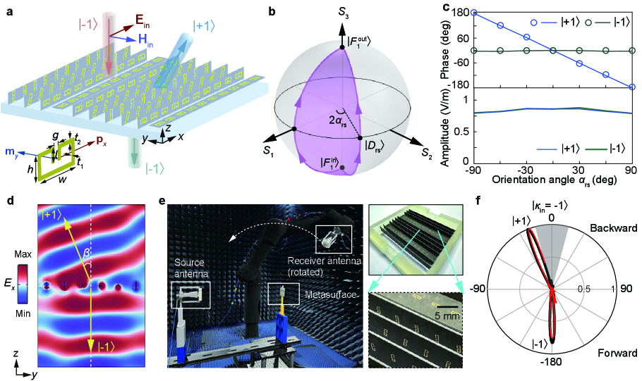
Figure 3: Wave deflection by the RS metasurface. (a) Schematic of the RS metasurface under the normally incident plane wave with linearly polarized electric field. The inset shows the structure of the meta-atom. (b) RS polarization evolution on the RS-sphere induced by the metasurface. (c) Theoretical RS geometric phase (symbols), simulated phase (solid lines), and simulated amplitude for the forward and backward scattering fields as a function of the orientation angle $\alpha_{\mathrm{rs}}$ of the RS dipole. (d) Simulated electric field scattered by the RS metasurface. (e) Experiment setup and the fabricated metasurface prototype. (f) Simulated and experimentally measured far-field intensity pattern. The shaded area marks the measurement blind zone [-15 deg, 15 deg] due to the source antenna obstruction.

RS metasurfaces and experiments

The RS phase can also emerge at artificial interfaces such as electromagnetic metasurfaces, due to the modulation of local electric and magnetic responses. To demonstrate this, we propose an RS metasurface comprising metallic split rings with the same geometric dimensions, as shown in Fig. 3a. The metasurface is under the normal incidence of a plane wave with linearly polarized electric and magnetic fields. The corresponding incident RS field is $\mathbf{F}_{1}^{\mathrm{in}}=(\hat{\mathbf{e}}_{x}-\mathrm{i}\hat{\mathbf{h}}_{y})Ee^{-\mathrm{i}k_{0}z-\mathrm{i}\omega t}$; its polarization state can be labelled by the RS spin as $\left|\kappa_{\mathrm{in}}=-1\right\rangle$. The incident wave excites an electric dipole $p_{x}$ and a magnetic dipole $m_{y}$ in the meta-atoms, forming a RS dipole $\mathbf{D}_{\mathrm{rs}}=p_{x}\hat{\mathbf{e}}_{x}+\mathrm{i}{m_{y}}\hat{\mathbf{h}}_{y}$ and generating scattering fields in forward and backward directions. The scattering RS field is $\mathbf{F}_{1}^{\text{out}}=(\hat{\mathbf{e}}_{x}+\mathrm{i}\kappa_{\text{out}}\hat{\mathbf{h}}_{y})Ee^{\mathrm{i}\kappa_{\text{out}}k_{0}z-\mathrm{i}\omega t}$ with polarization state $\left|\kappa_{\text{out}}=\pm 1\right\rangle$. Denoting the polarization evolution as $\left|\kappa_{\text{in}}\right\rangle\rightarrow\left|\kappa_{\text{out}}\right\rangle$, the RS phase emerges in the cross-polarized channel $|-1\rangle\rightarrow|+1\rangle$ but vanishes in the co-polarized channel $|-1\rangle\rightarrow|-1\rangle$.

Figure 3b shows the RS polarization evolution in the channel $|-1\rangle\rightarrow|+1\rangle$. The incident state $\left|F_{1}^{\text{in}}\right\rangle$ and backward scattering state $\left|F_{1}^{\text{out}}\right\rangle$ are represented by the south and north poles, respectively. The polarization state of the RS dipole $\mathbf{D}_{\mathrm{rs}}$, denoted as $\left|D_{\mathrm{rs}}\right\rangle$, is located on the equator. The orientation angle of $\mathbf{D}_{\mathrm{rs}}$ in the constitutive frame is $\alpha_{\mathrm{rs}}=\text{arctan}(\frac{\mathrm{i}m_{y}}{p_{x}})$. Rotating the meta-atoms around $x$ or $y$ direction will alter $\alpha_{\mathrm{rs}}$ (Supplementary Note IV) and change the azimuthal angle on the RS-sphere. The resulting RS phase is $\Phi_{\mathrm{rs}}=-2\alpha_{\mathrm{rs}}$. Notably, the PB phase vanishes in this case because the meta-atom rotation around $x$ or $y$ direction does not change the electric or magnetic polarization. Figure 3c shows the phases and amplitudes of the scattering fields as a function of the orientation angle $\alpha_{\mathrm{rs}}$ of the RS dipole $\mathbf{D}_{\mathrm{rs}}$. The simulated phases (solid lines) agree with the RS phase (circles) obtained by evaluating the solid angle in the RS-sphere. Notably, the phase of the backward scattering field $|+1\rangle$ exhibits a linear relationship with $\alpha_{\mathrm{rs}}$, while the phase of the forward scattering field $|-1\rangle$ is independent of $\alpha_{\mathrm{rs}}$. In addition, the scattering amplitudes remain approximately constant for different $\alpha_{\mathrm{rs}}$. These results indicate that the RS metasurface can enable Janus-type wavefront shaping and functionality.

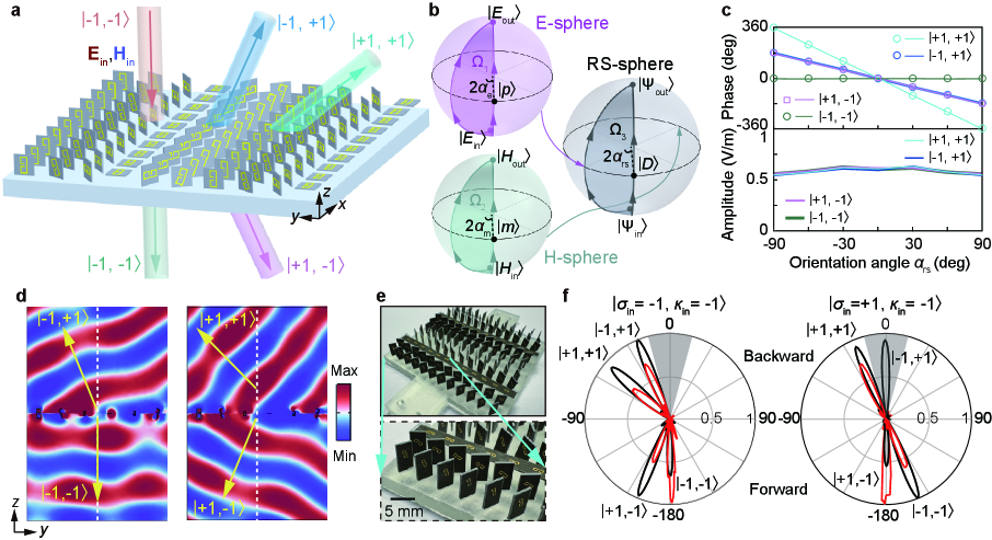
Figure 4: Wave deflection by the higher-order RS metasurface. (a) Schematic of the quadruplex RS meta-deflector under the normal incidence of a plane wave with LCP electric field. (b) 4D polarization evolution on the Poincaré hypersphere induced by the higher-order RS metasurface. (c) Theoretical geometric phase (symbols), simulated phase (solid lines), and simulated amplitude in four polarization evolution channels as a function of the orientation angle of RS dipole in the meta-atom. (d) Simulated electric field distribution of four output waves. (e) Fabricated metasurface prototype. (f) Simulated and experimentally measured far-field intensity pattern under orthogonal incidence. The shaded area marks the measurement blind zone [-15 deg, 15 deg] due to the source antenna obstruction.

The RS metasurface in Fig. 3a can generate RS phase gradient along $y$ direction, which can deflect the incident wave. Figure 3d shows the simulated electric field $E_{x}$ scattered by the RS metasurface. We note that only the backward scattering field is deflected into oblique direction, and the wavefront is consistent with the deflection angle $\beta=\arcsin(\frac{1}{k_{0}}\frac{\Delta\Phi_{\mathrm{rs}}}{\Delta y})$ predicted by the generalized Snell’s law [57]. The deflection direction can be reversed by flipping the RS spin (i.e., propagation direction) of the incident plane wave (Supplementary Note V). We conduct microwave experiments to verify the theory by using the experiment setup and metasurface in Fig. 3e (Methods). The measured far-field intensity scattered by the metasurface is shown as the red line in Fig. 3f, which agrees well with the simulation result denoted by the black line. Only the backward scattering lobe exhibits a deflection angle, confirming the validity of the theory.

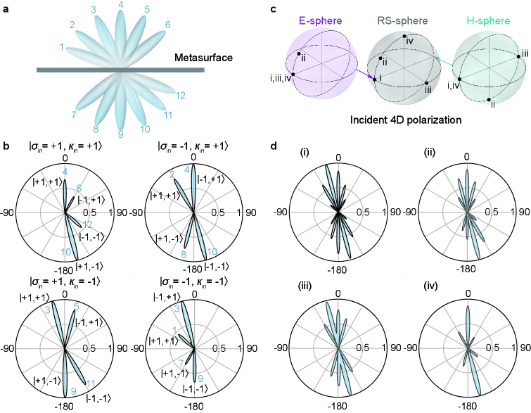
Figure 5: Reconfigurable wave deflection by the general RS metasurface. (a) Schematic of the multiplexed beam forming with twelve distinct output wavefronts. (b) Simulated far-field intensity patterns under the normal incidence of plane waves with orthogonal 4D polarizations. The lobes are labelled in accordance with (a). (c) Incident 4D polarizations (labelled as “i-iv”) for achieving reconfigurable far-field intensity patterns. (d) Far-field intensity patterns with different number of lobes induced by the incident polarizations “i-iv” in (c).

The synergy of RS and PB phases can enable high-dimensional wavefront manipulation. To demonstrate this, we consider the higher-order RS metasurface in Fig. 4a under the incidence of a plane wave with circularly polarized electric and magnetic fields. Compared to the metasurface in Fig. 3a, the meta-atoms here are rotated around the local $z$ axis, in addition to the rotation around the local $x$ or $y$ axis (Methods). The $z$-axis rotation induces electric and magnetic polarization evolutions, giving rise to the PB phase $\Phi_{\mathrm{pb}}$. Consequently, the metasurface generates scattering fields carrying the total geometric phase $\Phi_{\text{tot }}=\Phi_{\mathrm{pb}}+\Phi_{\mathrm{rs}}$. The incident wave field is $\bm{\Psi}_{\text{in}}=[\left(\hat{\mathbf{e}}_{x}+\mathrm{i}\sigma_{\text{in}}\hat{\mathbf{e}}_{y}\right)-\mathrm{i}(\hat{\mathbf{h}}_{y}-\mathrm{i}\sigma_{\text{in}}\hat{\mathbf{h}}_{x})]Ee^{-\mathrm{i}k_{0}z-\mathrm{i}\omega t}$, which carries the spins $\sigma_{\text{in }}=-1$ and $\kappa_{\text{in }}=-1$. Its electric, magnetic, and RS polarization states are represented by the south poles on the E-sphere, H-sphere, and RS-sphere, respectively, as shown in Fig. 4b. The incident wave excites the 4D dipole in the meta-atoms: $\mathbf{D}=\mathbf{p}+\mathrm{i}{\mathbf{m}}=[(p_{x}\hat{\mathbf{e}}_{x}+p_{y}\hat{\mathbf{e}}_{y})+{\mathrm{i}}(m_{y}\hat{\mathbf{h}}_{y}+m_{x}\hat{\mathbf{h}}_{x})]e^{-\mathrm{i}\omega t}$. The polarization states of the electric, magnetic, and RS dipoles are represented by $|p\rangle,|m\rangle$, and $\left|D_{\mathrm{rs}}\right\rangle$ on the equators with the azimuthal angles $2\alpha_{\mathrm{p}},2\alpha_{\mathrm{m}}$, and $2\alpha_{\mathrm{rs}}$, respectively. Here, $\alpha_{\mathrm{p}}\left(\alpha_{\mathrm{m}}\right)$ is the orientation angle of the electric (magnetic) dipole in the coordinate frame; $\alpha_{\mathrm{rs}}$ is the orientation angle of the RS dipole in the constitutive frame. The meta-atoms in Fig. 4a are designed to satisfy $\alpha_{\mathrm{p}}=\alpha_{\mathrm{rs}}$. The metasurface generates the scattering field $\bm{\Psi}_{\text{out }}=[(\hat{\mathbf{e}}_{x}+\mathrm{i}\sigma_{\text{out}}\hat{\mathbf{e}}_{y})+\mathrm{i}\kappa_{\text{out}}(\hat{\mathbf{h}}_{y}-\mathrm{i}\sigma_{\text{out}}\hat{\mathbf{h}}_{x})]Ee^{\mathrm{i}\kappa_{\text{out}}k_{0}z-\mathrm{i}\omega t}$, which has four polarization components $\left|\sigma_{\text{out}}=\pm 1,\kappa_{\text{out}}=\pm 1\right\rangle$, as shown in Fig. 4a. Correspondingly, there are four polarization evolution channels $\left|\sigma_{\mathrm{in}},\kappa_{\mathrm{in}}\right\rangle\rightarrow\left|\sigma_{\text{out}},\kappa_{\text{out}}\right\rangle$. Figure 4b shows the 4D polarization evolution in the channel $|-1,-1\rangle\rightarrow|+1,+1\rangle$ as an example. The resulting geometric phase is:

$$\Phi_{\mathrm{tot}}=\Phi_{\mathrm{pb}}+\Phi_{\mathrm{rs}}=\left(\sigma_{\mathrm{in}}-\sigma_{\mathrm{out}}\right)\alpha_{\mathrm{p}}+\left(\kappa_{\mathrm{in}}-\kappa_{\mathrm{out}}\right)\alpha_{\mathrm{rs}}.$$ (1)

Figure 4c shows the phases and amplitudes of the four output waves for different orientation angle $\alpha_{\mathrm{rs}}$. The simulated phases (solid lines) are consistent with the total geometric phases (symbols) given by the solid angles on the Poincaré hypersphere. The simulated amplitudes of different outputs are approximately equal and nearly independent of $\alpha_{\mathrm{rs}}$.

Figure 4d shows the simulated electric fields of the four output waves. The wavefronts are consistent with the deflection directions (yellow arrows) predicted based on the geometric phase gradient. Specifically, the output $|+1,+1\rangle$ exhibits the largest deflection angle; $|+1,-1\rangle$ and $|-1,+1\rangle$ exhibit the same deflection angle; $|-1,-1\rangle$ undergoes no deflection. The number of distinct output wavefronts can be increased by flipping the electric spin and RS spin of the incident wave (Supplementary Notes VI and VII). Figure 4e shows the fabricated metasurface sample comprising two supercells. The scattering far-field intensities under the incidence of the plane waves $\left|\sigma_{\mathrm{in}}=\pm 1,\kappa_{\mathrm{in}}=-1\right\rangle$ are shown in Fig. 4f. We notice that a total of eight output intensity lobes (four lobes in each case) emerge in six distinct directions, with consistency between the experimental (red lines) and simulation (black lines) results. Unlike the case in Fig. 4c, the intensities of different outputs are not equal due to the finite size of the metasurface.

The output wavefronts can be further increased by setting $\alpha_{\mathrm{p}}=\alpha_{\mathrm{m}}\neq\alpha_{\mathrm{rs}}$ for the RS metasurface in Fig. 4a. Under the incidence of the plane waves $\left|\sigma_{\mathrm{in}}=\pm 1,\kappa_{\mathrm{in}}=\pm 1\right\rangle$, this metasurface can generate twelve distinct output wavefronts propagating in different directions, as schematically shown in Fig. 5a. The simulated far-field intensity patterns are shown in Fig. 5b, where the intensity lobes are labelled in accordance with the numbers in Fig. 5a. As seen, the scattered far fields can propagate in twelve different directions, depending on the values of $\sigma_{\text{out}}$ and $\kappa_{\text{out}}$. Additionally, the number of distinct outputs can be dynamically reconfigured by employing the incident wave $\left|\Psi_{\text{in}}\right\rangle=\eta_{1}|+1,+1\rangle+\eta_{2}|+1,-1\rangle+\eta_{3}|-1,+1\rangle+\eta_{4}|-1,-1\rangle$ with varying 4D polarization. For example, by tuning the coefficients $\eta_{1-4}$ to obtain four different incident polarizations, denoted by the points “i-iv” on the Poincaré hypersphere in Fig. 5c, the metasurface can generate 12, 10, 8, and 6 far-field intensity lobes, as shown in Fig. 5d. These results demonstrate that the general RS metasurface can enable high-dimensional wavefront manipulations beyond the capabilities of conventional metasurfaces. The functionalities can be further enriched if time-varying or active components are introduced into the system [58, 59, 60, 61].

Discussion

In summary, we unravel a high-dimensional manifestation of the geometric phase induced by complete electromagnetic polarization evolution in the 4D RS Hilbert space. Beyond the conventional PB phase induced by electric or magnetic polarization evolution, we discover a new geometric phase—RS phase, which originates from the hybrid electric-magnetic polarization evolution and can emerge even in linearly polarized waves. The findings provide fundamental insights into the geometric nature of high-dimensional light-matter interactions and enable multiplexed wavefront shaping through the RS metasurfaces. The proposed mechanism applies to general electromagnetic waves including evanescent waves and complex structured waves. Our work broadens the geometric phase paradigm and introduces new degrees of freedom for light manipulation, which can facilitate multifunctional nanophotonic design and enhance communication capacity.

Methods

Poincaré hypersphere representation

The 4D electromagnetic polarization can be represented on the Poincaré hypersphere in Fig. 1a. The north and south poles of the E-sphere are $\left|N_{\mathrm{e}}\right\rangle=\frac{1}{\sqrt{2}}\left(\hat{\mathbf{e}}_{i}+\mathrm{i}\hat{\mathbf{e}}_{j}\right)$ and $\left|S_{\mathrm{e}}\right\rangle=\frac{1}{\sqrt{2}}\left(\hat{\mathbf{e}}_{i}-\mathrm{i}\hat{\mathbf{e}}_{j}\right)$, respectively. The north and south poles of the H-sphere are $\left|N_{\mathrm{m}}\right\rangle=\frac{1}{\sqrt{2}}(\hat{\mathbf{h}}_{j}-\mathrm{i}\hat{\mathbf{h}}_{i})$ and $\left|S_{\mathrm{m}}\right\rangle=\frac{1}{\sqrt{2}}(\hat{\mathbf{h}}_{j}+\mathrm{i}\hat{\mathbf{h}}_{i})$, respectively. Any 4D polarization state $|\Psi\rangle$ can be parameterized by six parameters ($\theta_{\mathrm{e}},\phi_{\mathrm{e}},\theta_{\mathrm{m}},\phi_{\mathrm{m}},\theta_{\mathrm{rs}},\phi_{\mathrm{rs}}$) as

$$|\Psi\rangle =\frac{1}{\sqrt{2}}\left[\cos\left(\frac{\theta_{\mathrm{rs}}}{2}\right)e^{-\mathrm{i}\frac{\phi_{\mathrm{rs}}}{2}}+\sin\left(\frac{\theta_{\mathrm{rs}}}{2}\right)e^{\mathrm{i}\frac{\phi_{\mathrm{rs}}}{2}}\right]\left|H_{\mathrm{rs}}\right\rangle$$ (2)

$$+\mathrm{i}\frac{1}{\sqrt{2}}\left[\cos\left(\frac{\theta_{\mathrm{rs}}}{2}\right)e^{-\mathrm{i}\frac{\phi_{\mathrm{rs}}}{2}}-\sin\left(\frac{\theta_{\mathrm{rs}}}{2}\right)e^{\mathrm{i}\frac{\phi_{\mathrm{rs}}}{2}}\right]\left|V_{\mathrm{rs}}\right\rangle,$$

where $\left|H_{\mathrm{rs}}\right\rangle=\cos\left(\frac{\theta_{\mathrm{e}}}{2}\right)e^{-\frac{\mathrm{i}\phi_{\mathrm{e}}}{2}}\left|N_{\mathrm{e}}\right\rangle+\sin\left(\frac{\theta_{\mathrm{e}}}{2}\right)e^{\frac{\mathrm{i}\phi_{\mathrm{e}}}{2}}\left|S_{\mathrm{e}}\right\rangle$ represents an arbitrary state on the E-sphere and $\left|V_{\mathrm{rs}}\right\rangle=\cos\left(\frac{\theta_{\mathrm{m}}}{2}\right)e^{-\frac{\mathrm{i}\phi_{\mathrm{m}}}{2}}\left|N_{\mathrm{m}}\right\rangle+\sin\left(\frac{\theta_{\mathrm{m}}}{2}\right)e^{\frac{\mathrm{i}\phi_{\mathrm{m}}}{2}}\left|S_{\mathrm{m}}\right\rangle$ represents an arbitrary state on the H-sphere. The representation of the electric (magnetic) polarization on the E-sphere (H-sphere) has been well established in the literature. The representation of the hybrid $\mathbf{E}$-$\mathbf{H}$ polarization on the RS-sphere can be understood by considering the RS vector $\mathbf{F}_{1}=E_{i}\hat{\mathbf{e}}_{i}+\mathrm{i}H_{j}\hat{\mathbf{h}}_{j}$ of paraxial waves as an example ($\mathbf{F}_{2}$ exhibits the same polarization and can be represented similarly). The temporal evolution of $\mathbf{F}_{1}$ traces out a polarization ellipse on the plane with the bases ($\hat{\mathbf{e}}_{i},\hat{\mathbf{h}}_{j}$), where the polarization ellipticity and orientation are determined by the relative magnitude and phase of $E_{i}$ and $H_{j}$. The polarization of $\mathbf{F}_{1}$ can be mapped to a point on the RS-sphere with the normalized RS Stokes vector $\left(S_{1},S_{2},S_{3}\right)$, where $S_{1}=\frac{\left|E_{i}\right|^{2}-\left|H_{j}\right|^{2}}{\left|E_{i}\right|^{2}+\left|H_{j}\right|^{2}},S_{2}=\frac{2\operatorname{Re}\left[E_{i}\left(\mathrm{i}H_{j}\right)^{*}\right]}{\left|E_{i}\right|^{2}+\left|H_{j}\right|^{2}}=\frac{2\operatorname{Im}\left[E_{i}H_{j}^{*}\right]}{\left|E_{i}\right|^{2}+\left|H_{j}\right|^{2}}$, and $S_{3}=\frac{-2\operatorname{Im}\left[E_{i}\left(\mathrm{i}H_{j}\right)^{*}\right]}{\left|E_{i}\right|^{2}+\left|H_{j}\right|^{2}}=\frac{2\operatorname{Re}\left[E_{i}H_{j}^{*}\right]}{\left|E_{i}\right|^{2}+\left|H_{j}\right|^{2}}$. Importantly, $S_{1}$ is determined by the relative amplitude of $E_{i}$ and $H_{j};S_{2}$ and $S_{3}$ are determined by the imaginary and real parts of the complex Poynting vector, respectively.

Some representative RS polarization states and corresponding $E_{i}$-$H_{j}$ relations are shown in Fig. S1. The points located at $\phi=0$ longitudinal line correspond to propagating waves in transparent media with a real Poynting vector. Specifically, the north and south poles denote the free-space propagating waves in opposite directions. The points on the equator represent purely evanescent waves with an imaginary Poynting vector, e.g., waves in lossless electric/magnetic plasma media. The remaining points on the sphere denote waves in lossy or gain media with a complex Poynting vector.

Numerical simulation

All the full-wave numerical simulations are performed with the package COMSOL Multiphysics. In the simulation of the metasurfaces in Figs. 3-5, we set the periods of unit cells along $x$ and $y$ directions to be $L_{x}=L_{y}=5.5\mathrm{\penalty 10000\ mm}$. The working frequency is 24 GHz. In each unit cell, the split ring has two arms with geometric parameters: $t_{1}=0.035\mathrm{\penalty 10000\ mm},t_{2}=0.15\mathrm{\penalty 10000\ mm},h=1\mathrm{\penalty 10000\ mm},w=2.3\mathrm{\penalty 10000\ mm},l=0.58\mathrm{\penalty 10000\ mm}$, and $g=0.27\mathrm{\penalty 10000\ mm}$ (refer to Fig. 3a for the definition of the geometric parameters). The split rings are made of copper with the electrical conductivity $\sigma=5.814\times 10^{7}\mathrm{\penalty 10000\ S}/\mathrm{m}$. To change the 4D dipole polarization of the meta-atom, we rotate the split ring around the $x,y$, and $z$ axis by angles $\alpha_{x},\alpha_{y}$, and $\alpha_{z}$, respectively. For the numerical demonstration in Fig. 3, each supercell comprises six split rings with the rotation angles $(\alpha_{x},\alpha_{y},\alpha_{z})$ in degrees: $(0,-90,0)$, $(0,-68,0)$, $(0,0,0)$, $(-90,0,0)$, $(0,180,0)$, and $(0,112,0)$. For the numerical demonstration in Fig. 4, each supercell comprises six split rings with the rotation angles $(\alpha_{x},\alpha_{y},\alpha_{z})$ in degrees: $(0,-90,-90)$, $(0,-68,-60)$, $(0,0,-30)$, $(-90,0,0)$, $(0,180,30)$, and $(0,112,60)$. For the numerical demonstration in Fig. 5, each supercell comprises six split rings with the rotation angles $(\alpha_{x},\alpha_{y},\alpha_{z})$ in degrees: $(0,82,-160)$, $(0,68,-120)$, $(0,45,-80)$, $(-45,0,-40)$, $(-90,0,0)$, $(-130,0,40)$, $(0,135,80)$, $(0,112,120)$, and $(0,96,160)$. To obtain the incident 4D polarizations “i-iv” in Fig. 5c, we set the coefficients ($\eta_{1}$, $\eta_{2}$, $\eta_{3}$, $\eta_{4}$)=($\frac{1}{2}$,$\frac{1}{2}$,$\frac{1}{2}$,$\frac{1}{2}$) for “i”, ($\frac{1}{\sqrt{3}}$,$\frac{1}{\sqrt{3}}$,$\frac{1}{\sqrt{3}}$,0) for “ii”, (0,$\frac{1}{\sqrt{2}}$,$\frac{1}{\sqrt{2}}$,0) for “iii”, and ($\frac{1}{\sqrt{2}}$,0,$\frac{1}{\sqrt{2}}$,0) for “iv”.

Experiment

The metasurfaces are fabricated on a Roger’s 5880 substrate with printed circuit board technology (thickness $t_{\mathrm{s}}=0.508\mathrm{\penalty 10000\ mm}$, height $h_{\mathrm{s}}=4\mathrm{\penalty 10000\ mm}$, relative permittivity $\varepsilon_{r}=2.2$, and loss $\operatorname{tangent}\tan\delta=0.0009$). Experimental characterization is performed in a microwave anechoic chamber to suppress multi-path effects. The setup comprises a linearly polarized transmitting horn antenna, a receiving horn antenna (Rx), and a vector network analyzer (VNA, Keysight PNA 5227B). Both antennas are positioned 1 m from the metasurface and connected to the two ports of the VNA via $50\Omega$ coaxial cables. By rotating the angular position of the Rx horn antenna with respect to the metasurface and measuring the transmitted/reflected signals by the VNA, the far-field scattering pattern of the metasurface is obtained. For the measurements in Fig. 4, wideband 3D-printed polarizers are mounted on the horn apertures to generate and detect circularly polarized waves. Prior to characterizing the metasurface, a background signal measurement is performed without the sample to capture the direct coupling between the source and receiver as well as other ambient contributions. The measured background signals are then used for calibration to minimize the contributions of these spurious signals to the measurement.

References

References

- [1] Pancharatnam, S. Generalized theory of interference, and its applications. Proc. Indian Acad. Sci. Sect. A 44, 247–262 (1956).
- [2] Berry, M. V. Quantal phase factors accompanying adiabatic changes. Proc. R. Soc. Lond. A 392, 45–57 (1984).
- [3] Shapere, A. & Wilczek, F. Geometric phases in physics (World scientific, 1989).
- [4] Cohen, E., Larocque, H., Bouchard, F., Nejadsattari, F., Gefen, Y. & Karimi, E. Geometric phase from Aharonov–Bohm to Pancharatnam–Berry and beyond. Nat. Rev. Phys. 1, 437–449 (2019).
- [5] Simon, B. Holonomy, the quantum adiabatic theorem, and Berry’s phase. Phys. Rev. Lett. 51, 2167–2170 (1983).
- [6] Aharonov, Y. & Anandan, J. Phase change during a cyclic quantum evolution. Phys. Rev. Lett. 58, 1593–1596 (1987).
- [7] Mead, C. A. The geometric phase in molecular systems. Rev. Mod. Phys. 64, 51–85 (1992).
- [8] Xiao, D., Chang, M.-C. & Niu, Q. Berry phase effects on electronic properties. Rev. Mod. Phys. 82, 1959–2007 (2010).
- [9] Liu, T., Qiang, X.-B., Lu, H.-Z. & Xie, X. Quantum geometry in condensed matter. Natl. Sci. Rev. 12, nwae334 (2025).
- [10] Tomita, A. & Chiao, R. Y. Observation of Berry’s topological phase by use of an optical fiber. Phys. Rev. Lett. 57, 937–940 (1986).
- [11] Bliokh, K. Y., Gorodetski, Y., Kleiner, V. & Hasman, E. Coriolis effect in optics: unified geometric phase and spin-Hall effect. Phys. Rev. Lett. 101, 030404 (2008).
- [12] Wang, S., Ma, G. & Chan, C. T. Topological transport of sound mediated by spin-redirection geometric phase. Sci. Adv. 4, eaaq1475 (2018).
- [13] Wang, J., Valligatla, S., Yin, Y., Schwarz, L., Medina-Sánchez, M., Baunack, S., Lee, C. H., Thomale, R., Li, S. & Fomin, V. M. Experimental observation of Berry phases in optical Möbius-strip microcavities. Nat. Photonics 17, 120–125 (2023).
- [14] Bliokh, K. Y., Rodríguez-Fortuño, F. J., Nori, F. & Zayats, A. V. Spin–orbit interactions of light. Nat. Photonics 9, 796–808 (2015).
- [15] Haldane, F. D. M. & Raghu, S. Possible realization of directional optical waveguides in photonic crystals with broken time-reversal symmetry. Phys. Rev. Lett. 100, 013904 (2008).
- [16] Wang, Z., Chong, Y., Joannopoulos, J. D. & Soljačić, M. Observation of unidirectional backscattering-immune topological electromagnetic states. Nature 461, 772–775 (2009).
- [17] Lu, L., Joannopoulos, J. D. & Soljačić, M. Topological photonics. Nat. Photonics 8, 821–829 (2014).
- [18] Ozawa, T., Price, H. M., Amo, A., Goldman, N., Hafezi, M., Lu, L., Rechtsman, M. C., Schuster, D., Simon, J. & Zilberberg, O. Topological photonics. Rev. Mod. Phys. 91, 015006 (2019).
- [19] Bliokh, K. Y., Alonso, M. A. & Dennis, M. R. Geometric phases in 2D and 3D polarized fields: geometrical, dynamical, and topological aspects. Rep. Prog. Phys. 82, 122401 (2019).
- [20] Song, Q., Odeh, M., Zúñiga-Pérez, J., Kanté, B. & Genevet, P. Plasmonic topological metasurface by encircling an exceptional point. Science 373, 1133–1137 (2021).
- [21] Cisowski, C., Götte, J. & Franke-Arnold, S. Colloquium: Geometric phases of light: Insights from fiber bundle theory. Rev. Mod. Phys. 94, 031001 (2022).
- [22] Fu, T., Zhang, R.-Y., Jia, S., Chan, C. & Wang, S. Near-field spin Chern number quantized by real-space topology of optical structures. Phys. Rev. Lett. 132, 233801 (2024).
- [23] Bomzon, Z., Biener, G., Kleiner, V. & Hasman, E. Space-variant Pancharatnam–Berry phase optical elements with computer-generated subwavelength gratings. Opt. Lett. 27, 1141–1143 (2002).
- [24] Yin, X., Ye, Z., Rho, J., Wang, Y. & Zhang, X. Photonic spin Hall effect at metasurfaces. Science 339, 1405–1407 (2013).
- [25] Wang, S., Wu, P. C., Su, V.-C., Lai, Y.-C., Chen, M.-K., Kuo, H. Y., Chen, B. H., Chen, Y. H., Huang, T.-T., Wang, J.-H., Lin, R.-M., Kuan, C.-H., Li, T., Wang, Z., Zhu, S. & Tsai, D. P. A broadband achromatic metalens in the visible. Nat. Nanotechnol. 13, 227–232 (2018).
- [26] Peng, J., Zhang, R.-Y., Jia, S., Liu, W. & Wang, S. Topological near fields generated by topological structures. Sci. Adv. 8, eabq0910 (2022).
- [27] Kim, G., Kim, Y., Yun, J., Moon, S.-W., Kim, S., Kim, J., Park, J., Badloe, T., Kim, I. & Rho, J. Metasurface-driven full-space structured light for three-dimensional imaging. Nat. Commun. 13, 5920 (2022).
- [28] Xiong, B., Liu, Y., Xu, Y., Deng, L., Chen, C.-W., Wang, J.-N., Peng, R., Lai, Y., Liu, Y. & Wang, M. Breaking the limitation of polarization multiplexing in optical metasurfaces with engineered noise. Science 379, 294–299 (2023).
- [29] Lin, D., Fan, P., Hasman, E. & Brongersma, M. L. Dielectric gradient metasurface optical elements. Science 345, 298–302 (2014).
- [30] Tymchenko, M., Gomez-Diaz, J. S., Lee, J., Nookala, N., Belkin, M. A. & Alù, A. Gradient nonlinear Pancharatnam-Berry metasurfaces. Phys. Rev. Lett. 115, 207403 (2015).
- [31] Devlin, R. C., Ambrosio, A., Rubin, N. A., Mueller, J. B. & Capasso, F. Arbitrary spin-to–orbital angular momentum conversion of light. Science 358, 896–901 (2017).
- [32] Yuan, Y., Zhang, K., Ratni, B., Song, Q., Ding, X., Wu, Q., Burokur, S. N. & Genevet, P. Independent phase modulation for quadruplex polarization channels enabled by chirality-assisted geometric-phase metasurfaces. Nat. Commun. 11, 4186 (2020).
- [33] Wang, B., Liu, W., Zhao, M., Wang, J., Zhang, Y., Chen, A., Guan, F., Liu, X., Shi, L. & Zi, J. Generating optical vortex beams by momentum-space polarization vortices centred at bound states in the continuum. Nat. Photonics 14, 623–628 (2020).
- [34] Xiao, W. & Wang, S. On-chip optical wavefront shaping by transverse-spin-induced Pancharatanam–Berry phase. Opt. Lett. 49, 1915–1918 (2024).
- [35] Pan, H., Chen, M. K., Tsai, D. P. & Wang, S. Nonreciprocal Pancharatnam-Berry metasurface for unidirectional wavefront manipulations. Opt. Express 32, 25632–25643 (2024).
- [36] Zeng, Y., Sha, X., Zhang, C., Zhang, Y., Deng, H., Lu, H., Qu, G., Xiao, S., Yu, S., Kivshar, Y. et al. Metalasers with arbitrarily shaped wavefront. Nature 643, 1240–1245 (2025).
- [37] Berry, M. V. The adiabatic phase and Pancharatnam’s phase for polarized light. J. Mod. Opt. 34, 1401–1407 (1987).
- [38] Bhandari, R. & Samuel, J. Observation of topological phase by use of a laser interferometer. Phys. Rev. Lett. 60, 1211–1213 (1988).
- [39] Barnett, S. M. Optical Dirac equation. New J. Phys. 16, 093008 (2014).
- [40] Alpeggiani, F., Bliokh, K., Nori, F. & Kuipers, L. Electromagnetic helicity in complex media. Phys. Rev. Lett. 120, 243605 (2018).
- [41] Nye, J. F. & Hajnal, J. The wave structure of monochromatic electromagnetic radiation. Proc. R. Soc. Lond. A 409, 21–36 (1987).
- [42] Kemp, C. J., Cooper, N. R. & Ünal, F. N. Nested-sphere description of the N-level Chern number and the generalized Bloch hypersphere. Phys. Rev. Res. 4, 023120 (2022).
- [43] Zhang, Z., Zhao, H., Wu, S., Wu, T., Qiao, X., Gao, Z., Agarwal, R., Longhi, S., Litchinitser, N. M. & Ge, L. Spin–orbit microlaser emitting in a four-dimensional Hilbert space. Nature 612, 246–251 (2022).
- [44] Weber, H. Die partiellen Differential-Gleichungen der mathematischen Physik nach Riemann’s Vorlesungen (F. Vieweg & sohn, 1901).
- [45] Silberstein, L. Elektromagnetische grundgleichungen in bivektorieller behandlung. Ann. Phys. (Berlin) 327, 579–586 (1907).
- [46] Silberstein, L. Nachtrag zur abhandlung über „elektromagnetische grundgleichungen in bivektorieller behandlung”. Ann. Phys. (Berlin) 329, 783–784 (1907).
- [47] Bialynicki-Birula, I. Photon wave function. Prog. Opt. 36, 245–294 (1996).
- [48] Bialynicki-Birula, I. & Bialynicka-Birula, Z. The role of the riemann–silberstein vector in classical and quantum theories of electromagnetism. J. Phys. A: Math. Theor. 46, 053001 (2013).
- [49] Bliokh, K. Y., Bekshaev, A. Y. & Nori, F. Dual electromagnetism: helicity, spin, momentum and angular momentum. New J. Phys. 15, 033026 (2013).
- [50] Neugebauer, M., Eismann, J. S., Bauer, T. & Banzer, P. Magnetic and electric transverse spin density of spatially confined light. Phys. Rev. X 8, 021042 (2018).
- [51] Wang, S., Hou, B., Lu, W., Chen, Y., Zhang, Z. & Chan, C. T. Arbitrary order exceptional point induced by photonic spin–orbit interaction in coupled resonators. Nat. Commun. 10, 832 (2019).
- [52] Shi, P., Du, L., Li, C., Zayats, A. V. & Yuan, X. Transverse spin dynamics in structured electromagnetic guided waves. Proc. Natl. Acad. Sci. U.S.A. 118, e2018816118 (2021).
- [53] Eismann, J., Nicholls, L., Roth, D., Alonso, M. A., Banzer, P., Rodríguez-Fortuño, F., Zayats, A., Nori, F. & Bliokh, K. Transverse spinning of unpolarized light. Nat. Photonics 15, 156–161 (2021).
- [54] Vernon, A. J., Golat, S., Rigouzzo, C., Lim, E. A. & Rodriguez-Fortuno, F. J. A decomposition of light’s spin angular momentum density. Light Sci. Appl. 13, 160 (2024).
- [55] Golat, S., Vernon, A. J. & Rodríguez-Fortuño, F. J. The electromagnetic symmetry sphere: a framework for energy, momentum, spin and other electromagnetic quantities. Preprint at https://arxiv.org/abs/2405.15718 (2024).
- [56] Jackson, J. D. Classical electrodynamics (John Wiley & Sons, 1999).
- [57] Yu, N., Genevet, P., Kats, M. A., Aieta, F., Tetienne, J.-P., Capasso, F. & Gaburro, Z. Light propagation with phase discontinuities: generalized laws of reflection and refraction. Science 334, 333–337 (2011).
- [58] Zhang, L., Chen, X. Q., Liu, S., Zhang, Q., Zhao, J., Dai, J. Y., Bai, G. D., Wan, X., Cheng, Q., Castaldi, G., Galdi, V. & Cui, T. J. Space-time-coding digital metasurfaces. Nat. Commun. 9, 4334 (2018).
- [59] Shaltout, A. M., Shalaev, V. M. & Brongersma, M. L. Spatiotemporal light control with active metasurfaces. Science 364, eaat3100 (2019).
- [60] Galiffi, E., Tirole, R., Yin, S., Li, H., Vezzoli, S., Huidobro, P. A., Silveirinha, M. G., Sapienza, R., Alù, A. & Pendry, J. B. Photonics of time-varying media. Adv. Photonics 4, 014002 (2022).
- [61] Tirole, R., Vezzoli, S., Galiffi, E., Robertson, I., Maurice, D., Tilmann, B., Maier, S. A., Pendry, J. B. & Sapienza, R. Double-slit time diffraction at optical frequencies. Nat. Phys. 19, 999–1002 (2023).