Real-Time Rendering of Dynamic Line Sets using Voxel Ray Tracing

Abstract

Real-time rendering of dynamic line sets is relevant in many visualization tasks, including unsteady flow visualization and interactive white matter reconstruction from Magnetic Resonance Imaging. High-quality global illumination and transparency are important for conveying the spatial structure of dense line sets, yet remain difficult to achieve at interactive rates. We propose an efficient voxel-based ray-tracing framework for rendering large dynamic line sets with ambient occlusion and ground-truth transparency. The framework introduces a voxelization algorithm that supports efficient construction of acceleration structures for both voxel cone tracing and ray tracing. To further reduce per-frame preprocessing cost, we developed a voxel-based culling method that restricts acceleration structure construction to camera-visible voxels. Together, these contributions enable high-quality, real-time rendering of large-scale dynamic line sets with physically accurate transparency. The results show that our method outperforms the state of the art in quality and performance when rendering (semi-)opaque dynamic line sets.

<ccs2012> <concept> <concept_id>10010147.10010371.10010372.10010377</concept_id> <concept_desc>Computing methodologies Visibility</concept_desc> <concept_significance>500</concept_significance> </concept> <concept> <concept_id>10010147.10010371.10010372.10010374</concept_id> <concept_desc>Computing methodologies Ray tracing</concept_desc> <concept_significance>500</concept_significance> </concept> <concept> <concept_id>10010147.10010371.10010372.10010373</concept_id> <concept_desc>Computing methodologies Rasterization</concept_desc> <concept_significance>500</concept_significance> </concept> <concept> <concept_id>10003120.10003145.10003147.10010364</concept_id> <concept_desc>Human-centered computing Scientific visualization</concept_desc> <concept_significance>500</concept_significance> </concept> </ccs2012>

[500]Computing methodologies Visibility [500]Computing methodologies Ray tracing [500]Computing methodologies Rasterization [500]Human-centered computing Scientific visualization

1 Introduction

Real-time rendering of 3D line sets has many applications in scientific visualization and in the game industry. While some line sets are inherently static, others are dynamic: they vary over time as a result of a simulation or user interaction. Visualizing dynamic line sets becomes essential when dealing with time-varying flow data [MLP^∗10], particle trajectories, hair and fur simulation [WBK^∗07] and for enabling user interactions such as segmenting diffusion MRI whole brain tractograms into distinct white matter bundles [ASH^∗09, SSA^∗08, CWF^∗14] or real-time tractography [CWF^∗14]. Global illumination effects such as ambient occlusion and soft shadows facilitate depth and shape perception [DRN^∗17], while transparency is used to visualize otherwise occluded structures [KNM^∗20]. Rendering global illumination and transparency in real-time is challenging, particularly when dealing with large, dense line sets. Various rendering techniques have been proposed to address these issues for static line sets by pre-computing various acceleration structures. [KRW18, GG20, WMZ^∗20, McG20, SM04], When rendering dynamic line sets, however, there is limited to no opportunity for precomputation.

Global illumination in the context of line rendering is tackled, among others, using Ray-Tracing [WMZ^∗20], Sparse Voxel Octrees [McG20] or Screen-Space techniques [EHS12]. Literature has demonstrated that Voxel Cone Tracing [CNS^∗11] is well suited for rendering soft shadows and ambient occlusion for dense line sets and molecular datasets [KRW18, GG20, SGG15, HGVV16]. Voxel Cone Tracing has the advantage of having great performance while providing close to ground truth ambient occlusion quality. Voxel Cone Tracing relies on an acceleration structure called an occupancy pyramid [HGVV16]: a 3D texture hierarchy where each voxel contains the occupancy of overlapping primitives.

To construct the occupancy pyramid for dynamic datasets, geometric primitives are usually voxelized on the fly [CNS^∗11, SGG15, HGVV16]. Line rendering literature has shown that voxelization of line primitives can be used to create an occupancy pyramid that produces high-quality results when used for Voxel Cone Tracing[GG20, KRW18]. However, since line radius is not taken into account during voxel traversal, these voxelizations are not conservative, resulting in artifacts when used as the basis for ray-tracing[KRW18]. Molecular visualization literature computes the occupancy pyramid on the fly on the GPU for spherical[SGG15, HGVV16] and short cylindrical [HGVV16] primitives by sampling the signed distance function (SDF) for all voxels in the primitive’s Axis Aligned Bounding Box (AABB). AABBs, however, do not form a tight fit around long, thin, non-axis aligned lines, resulting in excessive sampling and reduced performance.

While recent line rendering literature gravitates towards voxel based ambient occlusion, it is more divided when it comes to the topic of visibility and transparency. Visibility remains a key challenge in rendering large line sets with very high depth complexity, where even standard opaque rasterization renders at non-interactive frame rates. Accurate transparency rendering techniques such as Depth Peeling [Eve01] or Per-Pixel Linked-Lists [YHGT10] only add to the performance overhead and are therefore impractical in real time. Culling strategies such as Hierarchical Culling[GRDE10, GG20] may be used to reduce the rasterization cost and can be used in conjunction with a K-Buffer to render accurate transparency, but comes at the cost of sorting all data every frame, which is expensive for large datasets[GG20].

Image-order methods try to address visibility using acceleration structures such as Bounding Volume Hierarchies [WMZ^∗20] or voxel-based representations [McG20, GG20, SM04] to accelerate ray-primitive intersections. However, since most state of the art line-rendering literature precomputes their acceleration structures, they are not directly applicable to the rendering of dynamic line sets [GG20, WMZ^∗20, McG20, KRW18, SM04].

Precomputed or not, to our knowledge no literature thus far takes advantage of the occupancy pyramid to accelerate rendering beyond Voxel Cone Tracing. Since it provides a proxy for occupancy, it can be used for primitive culling and empty space skipping.

In this work, we present an efficient rendering pipeline for high quality ray-tracing of dynamic line sets without pre-computation. We achieve real-time performance by leveraging a fast conservative voxelization scheme to construct an occupancy pyramid every frame, which is used to accelerate the remainder of the rendering pipeline. Based on the occupancy pyramid, volume rendering is used to determine the visible voxel set: i.e. the voxels that are visible from the camera’s current perspective. To accelerate per-frame preprocessing, per-voxel fragments lists are computed for just the visible voxel set, saving memory and performance. To accelerate shading, we compute ambient occlusion and direct shadowing terms in voxel space for just the visible voxel set. Finally, ray-tracing itself can be accelerated by using the occupancy pyramid as an octree to employ empty-space skipping. While this work presents a method to accelerate rendering of dynamic line sets, it could be extended to render almost any geometric primitive. To summarize, our main contribution is a high performance ray-traced rendering pipeline, which is made possible by:

• A GPU-based method for efficient and high-quality conservative voxelization of capsule primitives.

• A culling approach. By only constructing fragment lists for visible voxels, we save memory and increase performance.

• A voxel-based ray-tracing technique that renders ground truth transparency with high performance for semi-opaque line sets.

2 Related work

Our work is closely related to research in line voxelization and transparency techniques.

2.1 Voxelization of Line Sets

Voxelization of line segments has been a longstanding topic in computer graphics. An early influential algorithm is Bresenham’s line drawing algorithm [Bre65], which may be extended to 3D for voxelization. While Bresenham’s algorithm produces a single-pixel width line, it is not conservative, i.e. not all pixels/voxels intersected by the line are recognized. Xiaolin Wu [Wu91] proposed a method to rasterize anti-aliased lines, removing the staircasing effect at the cost of being more expensive than Bresenham. Amanatides & Woo’s Digital Differential Analyzer (DDA) algorithm [AW^∗87] provides a conservative voxelization for infinitely thin line segments that is widely used in ray-tracing today. However, none of these algorithm guarantee a conservative voxelization of a line segment with a radius, limiting their usefulness when building ray-tracing acceleration structures.

Voxelization of line segments can be used to generate an occupancy pyramid to enable voxel cone tracing, as is shown by Kanzler et al. [KRW18] and Groß and Gumhold [GG20], who respectively use rounded cone and cylinder primitives during rendering, but infinitely thin lines during voxelization. While both show how non-conservative voxelization of dense line sets can generate high quality occupancy pyramids, Kanzler et al. [KRW18] show it leads to missing-segment artifacts when used as the basis for ray-tracing and address this by sampling all voxel neighbors. We will show how conservative voxelization addresses these artifacts, while being less expensive than sampling the voxel neighborhood.

Dynamic molecular simulation methods generate an occupancy pyramid every frame in order to enable voxel cone tracing for simulated data [SGG15, HGVV16]. Staib et al. [SGG15] voxelize spherical particles by rendering planar slices to a 3D texture, using multi-sampling to create a conservative, anti-aliased voxelization. Hermosilla et al. [HGVV16] voxelize molecules that consist of atoms and bonds, modeled by sphere and cylinder primitives, respectively. Occupancy is estimated by evaluating the primitive’s signed distance function at the center of each voxel within the primitive’s axis aligned bounding box. Like Hermosilla et al. [HGVV16] and Hsieh et al. [HCTS10] we use signed distance functions to estimate occupancy. However, since our line sets contain line segments that may span many voxels, it can be expensive to evaluate all voxels within the primitive’s axis aligned bounding box. To improve performance for conservative voxelization of line primitives, we present a voxel traversal algorithm that scales better with line segment length.

2.2 Transparency

Accurate transparency requires compositing all geometry in visibility order, which is difficult to achieve in real-time. There are two key strategies of resolving transparency: object-order techniques usually employ order independent transparency techniques to capture all fragments per pixel, while image-order techniques build acceleration structures to accelerate ray-primitive intersections.

Transparency may be resolved using depth peeling [Eve01], by rasterizing all geometry as many times as the maximum depth complexity. Yet, for dense line sets with high depth complexity, achieving real-time performance using depth peeling is infeasible. To improve performance, multiple fragments may be captured per pixel in a single rasterization pass using variants of the A-Buffer [Car84]. A key challenge in A-Buffer techniques is that the number of fragments per pixel is not known in advance, making total memory cost unbounded and fragment write locations indeterminate.

Per-Pixel Linked Lists [YHGT10] may be used to capture all fragments by allowing linked lists to be created on the GPU. This introduces a significant memory overhead by storing a node pointer along with every fragment, which may be reduced by using fragment pages [Cra10]. The Linearized Layered Fragment Buffer [KLZ12] instead captures all fragments in two rendering passes. The first pass computes per-pixel fragment counts, which are converted into per-pixel memory offsets by means of a parallel prefix sum [HG12]. A secondary rendering pass is then used to capture all fragments into contiguous memory. Because these methods capture all fragments per pixel, they introduce a substantial memory and bandwidth overhead for scenes with high depth-complexity. Furthermore, while these methods capture all fragments, they still need to be sorted in order to produce correct transparency. Because generally more fragments are generated than there are primitives, sorting fragments is generally more expensive than sorting primitives.

Bavoil et al. takes another A-Buffer approach with their K-Buffer [BCL^∗07]: by resolving just the first $k$ closest primitives, they ensure bounded memory at the cost of insertion sorting each incoming fragment using global atomics. The K-Buffer was extended by Groß and Gumhold [GG20] who render close to ground truth transparency for large line sets with bounded memory, at the expense of sorting all primitives relative to the camera every frame.

In our work, we extend the Linearized Layered Fragment Buffer [KLZ12] into the voxel domain by employing a two-pass voxelization scheme to capture per-voxel fragment lists. By only capturing per-voxel fragment lists for the voxels visible to the camera, we save memory and increase performance.

Next to the well established rasterization techniques, image-order methods are a more recent addition to real-time line rendering literature. Schussman and Ma [SM04] opt for a per-voxel spherical harmonics representation of large dense line sets, which can be efficiently volume rendered. Kanzler et al. [KRW18] compute a voxel-based line segment quantization and a level of detail hierarchy that can be efficiently ray-traced, enabling rendering of large line sets with transparency. McGraw [McG20] uses an Octree to accelerate ray casting of line segments. Because they are represented by their Signed Distance Function (SDF), high quality interpolated line segments can be rendered with ray-cast shadows. Wald et al. [WMZ^∗20] repurposed GPU ray-tracing hardware to accelerate ray-tracing of dense line sets. Our method is most similar to that of Kanzler et al. [KRW18] and improves on their method by efficiently constructing the A-Buffer and using conservative voxelization to render high-quality semi-opaque dynamic line sets.

3 Voxel Ray Tracing

This section describes the rendering pipeline that enables real-time rendering of dynamic line sets with ambient occlusion and transparency. An overview of the pipeline is provided in Figure 1.

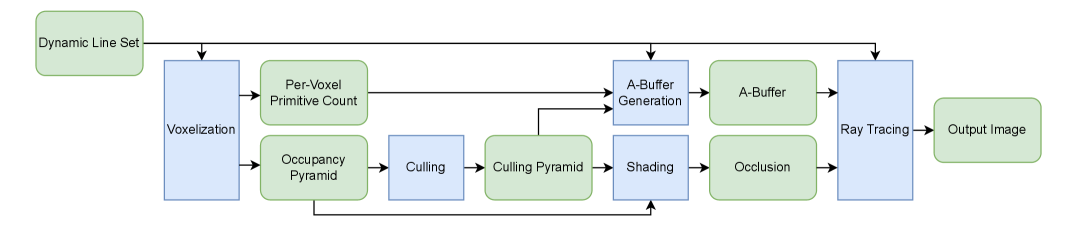
Figure 1: Schematic overview of the rendering pipeline and its intermediate outputs. Each step in the pipeline, represented by blue blocks, is described in sections 3.1-3.5. Green blocks represent (intermediate) data structures, while arrows show the in/outputs of each pipeline step.

Each line segment within each polyline of each dynamic line set is represented by a Quilez-style capsule primitive [Qui13, Qui08] during both voxelization and ray-tracing. The capsule primitive is chosen since it links adjacent line segments together without leaving gaps. As the first step of the rendering pipeline, all line segments undergo Voxelization (Section 3.1) using our efficient conservative voxelization algorithm. Voxelization quality is improved with our additions to signed distance field based occupancy estimation [HCTS10, HGVV16]. Next, by adapting standard volume rendering techniques, voxel-based Culling (Section 3.2) is used to determine the camera-visible voxels. We propose that during the A-Buffer Generation (Section 3.3) the per-voxel fragment lists are populated for just the camera-visible voxels, extending the Linearized Layered Fragment Buffer [KLZ12] into the voxel domain, while improving the performance of the secondary rendering pass. Shading is evaluated using Voxel Cone Tracing [CNS^∗11] in the Shading step (Section 3.4). Finally, we improve on the Voxel-based Line Raycasting method [KRW18] and render ground truth transparency with our voxel-based Ray-Tracing (Section 3.5).

3.1 Voxelization

To enable voxel cone tracing for dynamic line sets, we voxelize the entire line set every frame to generate the occupancy pyramid. Each voxel in the occupancy pyramid represents the volume fraction that is occupied by the line set. To use the voxelization for ray tracing, we rely on our conservative voxel traversal algorithm to ensure all capsule-voxel intersections are captured. For each intersection, we increment the per-voxel intersection count and estimate voxel occupancy using our clipped capsule signed distance function.

During voxelization, each line segment, described by its vertices $\mathbf{v_{0}}$ and $\mathbf{v_{1}}$, is treated as a capsule primitive with radius $r$. Our algorithm traverses along the axis corresponding with the largest-magnitude component, i.e. $x$, $y$ or $z$, of the line delta $\mathbf{d}=\mathbf{v_{1}}-\mathbf{v_{0}}$. At each iteration, the voxels along the two remaining (minor) axes ar voxelized. Unlike DDA, this traversal guarantees conservatism for capsule primitives, while improving performance by visiting fewer voxels than axis-aligned bounding box (AABB) voxelization. Figure 2 shows a schematic overview of the voxel traversal.

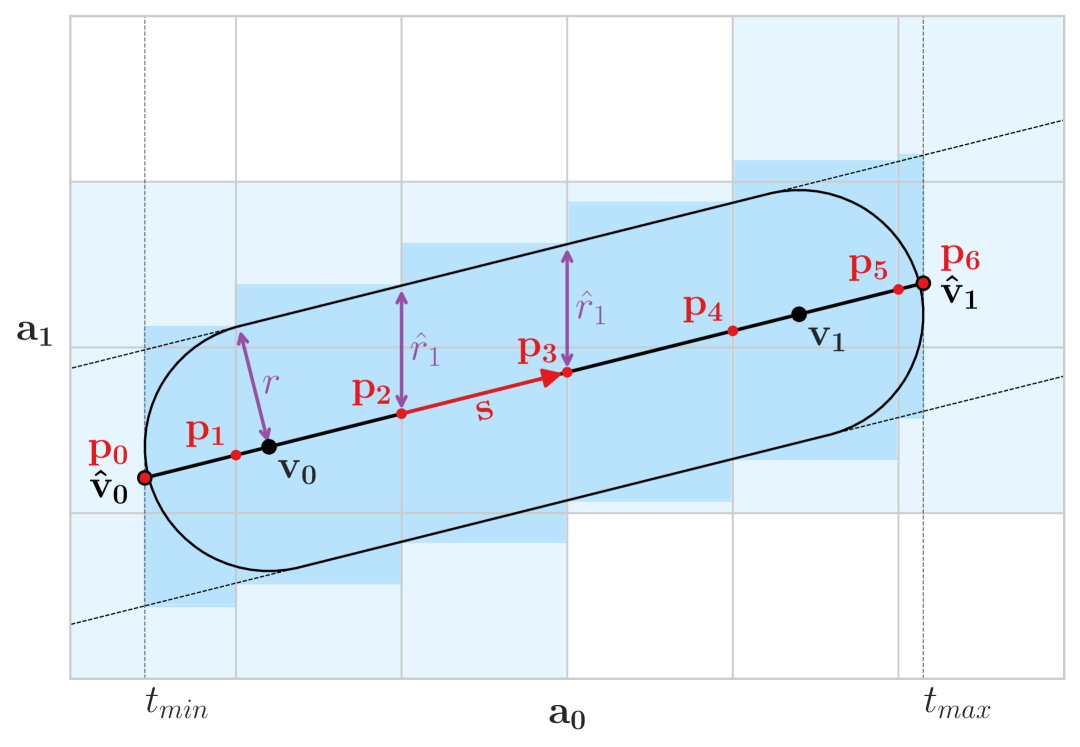
Figure 2: Illustration of our voxel traversal scheme, shown in 2D. The algorithm traverses axis $a_{0}$, visiting points $\mathbf{p_{0}}$-$\mathbf{p_{6}}$. For every consecutive pair of points a bounding box (dark blue) is computed along the minor axes $a_{1},a_{2}$ using the projected radii $\hat{r}_{1},\hat{r}_{2}$. All intersected voxels (light blue) are voxelized. See the text for details.

We first rank the vector components of line delta $\mathbf{d}$ based on their absolute magnitude to obtain axis index vector $\mathbf{a}=(a_{0},a_{1},a_{2})$ where $a_{i}\in\{x,y,z\}$. After ranking, $a_{0}$ contains the vector component index of the major axis and $a_{1},a_{2}$ contain the indices of the two minor axes. To simply traversal, we swap vertices $\mathbf{v_{0}}$ and $\mathbf{v_{1}}$ when the major axis is negative. By normalizing $\mathbf{d}$ relative to its largest vector component $d_{a_{0}}$, we obtain step vector $\mathbf{s}=\mathbf{d}/d_{a_{0}}$, as the vector from one major axis voxel boundary to the next. To capture the capsule ending caps, we extend the line segment in both directions with $\mathbf{s}\cdot r$ to obtain the extended vertices $\mathbf{\hat{v}_{0}}$ and $\mathbf{\hat{v}_{1}}$.

To capture the capsule radius along the minor axes $a_{1},a_{2}$, we compute the projected radii $\hat{r}_{1},\hat{r}_{2}$ on those axes, using:

$$\hat{r}_{i} =\dfrac{r}{\sqrt{1-\left(d_{a_{i}}/\left\|\mathbf{d}\right\|\right)^{2}}}\quad\text{where }i\in 1,2.$$ (1)

We traverse along the major axis $a_{0}$, from extended vertex $\mathbf{\hat{v}_{0}}$ to extended vertex $\mathbf{\hat{v}_{1}}$ and visiting every voxel boundary in between. For every consecutive pair of voxel intersection points along the major axis $a_{0}$, defined as $\mathbf{p_{n}}$ and $\mathbf{p_{n+1}}$, a 2D bounding box is computed along the minor axes $a_{1},a_{2}$ using radii $\hat{r}_{1},\hat{r}_{2}$ and every voxel that overlaps with this bounding box is visited. The voxel traversal pseudocode is given in Algorithm 1.

$t_{min}\leftarrow\hat{v}_{0,a_{0}}$ // major axis component of $\hat{v}_{0}$

$t_{max}\leftarrow\hat{v}_{1,a_{0}}$ // major axis component of $\hat{v}_{1}$

$t_{0}\leftarrow t_{min}$

$\mathbf{p_{0}}\leftarrow\mathbf{\hat{v}_{0}}$

while $t_{0}<t_{max}$ do

    // Compute next intersection point

    $t_{1}\leftarrow\min(t_{max},\text{floor}(t_{0}+1))$

    $\mathbf{p_{1}}\leftarrow\mathbf{\hat{v}_{0}}+\mathbf{s}(t_{1}-t_{min})$

   

    // Define 2D box to voxelize

    $j_{min}\leftarrow\text{int}(\min(p_{0,a_{1}},p_{1,a_{1}})-\hat{r}_{1})$

    $j_{max}\leftarrow\text{int}(\max(p_{0,a_{1}},p_{1,a_{1}})+\hat{r}_{1})$

    $k_{min}\leftarrow\text{int}(\min(p_{0,a_{2}},p_{1,a_{2}})-\hat{r}_{2})$

    $k_{max}\leftarrow\text{int}(\max(p_{0,a_{2}},p_{1,a_{2}})+\hat{r}_{2})$

   

    // Visit all voxels within 2D box

    for $j=j_{min}$ to $j_{max}$, $k=k_{min}$ to $k_{max}$ do

       $\mathbf{C}_{a_{0}}=\text{int}(t_{0})$, $\mathbf{C}_{a_{1}}=j$, $\mathbf{C}_{a_{2}}=k$

       Visit($\mathbf{C}$)

      

    end for

   

    // Move to next intersection point

    $t_{0}\leftarrow t_{1}$

    $\mathbf{p_{0}}\leftarrow\mathbf{p_{1}}$

   

end while

Algorithm 1 Conservative Capsule Voxelization

Our capsule voxelization algorithm has a theoretical advantage over axis-aligned bounding box voxelization. Depending on the line orientation relative to the voxel grid, AABB voxelization exhibits linear, quadratic, or cubic time complexity. Like DDA voxelization, our capsule voxelization method scales linearly with segment length, regardless of segment orientation. Given that in most line sets all line orientations are represented, our method should outperform AABB voxelization for longer line segments.

Using our capsule voxel traversal to iterate over all capsule-voxel intersections, we compute the base level of the occupancy pyramid by accumulating occupancy for each visited voxel. No closed-form expression capturing capsule-voxel intersection volume exists. Therefore we approximate occupancy using the signed distance function of our primitive, as in [HCTS10, HGVV16].

However, when representing each line segment in a polyline as a capsule, its endpoints will overlap, resulting in spherical artifacts at each interior vertex of each polyline. This results in an unwanted overestimation of occupancy, especially when vertices are densely packed together. To prevent the overlapping geometry to affect the voxelization, we follow Groß et al. [GG20] and define a clipping plane normal $\mathbf{n_{i}}$ as the tangent of vertex $\mathbf{v_{i}}$ computed using the central difference. We extend the Quilez capsule SDF [Qui08] to create the clipped capsule SDF shown in Algorithm 2, which computes the signed distance from point $\mathbf{p}$ to the clipped capsule with vertices $\mathbf{v_{0}},\mathbf{v_{1}}$, corresponding clipping planes $\mathbf{n_{0}},\mathbf{n_{1}}$ and radius $r$.

Function ClippedCapsuleSDF($\mathbf{p},\mathbf{v_{0}},\mathbf{v_{1}},\mathbf{n_{0}},\mathbf{n_{1}},r$):

    $\mathbf{d}\leftarrow\mathbf{v_{1}}-\mathbf{v_{0}}$

    $\mathbf{pv_{0}}\leftarrow\mathbf{p}-\mathbf{v_{0}}$

    $\mathbf{pv_{1}}\leftarrow\mathbf{p}-\mathbf{v_{1}}$

    $h\leftarrow\text{clamp}\left(\left(\mathbf{pv_{0}}\cdot\mathbf{d}\right)/\left(\mathbf{d}\cdot\mathbf{d}\right),0,1\right)$

   

    $sdf_{capsule}\leftarrow\|\mathbf{pv_{0}}-\mathbf{d}\cdot h\|-r$

    $sdf_{n_{0}}\leftarrow-\mathbf{pv_{0}}\cdot\mathbf{n_{0}}$

    $sdf_{n_{1}}\leftarrow\mathbf{pv_{1}}\cdot\mathbf{n_{1}}$

   

    return $\max(sdf_{capsule},sdf_{n_{0}},sdf_{n_{1}})$

   

Algorithm 2 Clipped Capsule Signed Distance Function

While the clipped capsule signed distance function can be used for approximating occupancy for capsules with large radii relative to voxel size, aliasing is introduced when the radius is smaller than half the voxel size. To reduce aliasing for small radii, we adapt Phone Wire Anti-Aliasing (PWAA) [Per12], which reduces aliasing when rendering thin lines by clamping the radius to the pixel size and fading alpha towards zero. We adapt PWAA to our clipped capsule signed distance in the voxel domain, by clamping the tube radius to a minimum value $r_{min}$ and correcting for the radius difference in the occupancy estimation. The completed occupancy estimation is shown in Algorithm 3 and visualized in Figure 3.

Function CapsuleOccupancy($\mathbf{p},\mathbf{v_{0}},\mathbf{v_{1}},\mathbf{n_{0}},\mathbf{n_{1}},r,r_{min}$):

    $r_{clamp}\leftarrow\max(r,r_{min})$

    $r_{correction}=(r/r_{clamp})^{2}$

   

    // Compute Occupancy from SDF

    $sdf\leftarrow\text{ClippedCapsuleSDF}(\mathbf{p},\mathbf{v_{0}},\mathbf{v_{1}},\mathbf{n_{0}},\mathbf{n_{1}},r_{clamp})$

    $occupancy=\text{clamp}(0.5-sdf,0,1)$

   

    return $occupancy\cdot r_{correction}$

Algorithm 3 Clipped Capsule Occupancy Estimation

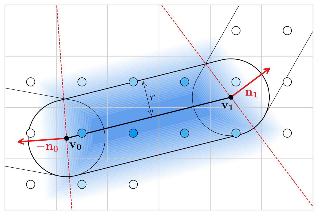
Figure 3: Illustration of the SDF-based occupancy estimation, shown in 2D. To compute the occupancy for a given capsule-voxel intersection, the clipped capsule occupancy function (Algorithm 3, shown as the blue gradient) is sampled at the center of each intersecting voxel (filled white-blue circles). See text for more details.

To construct the base level of the occupancy pyramid, each GPU thread voxelizes a single line segment at a time, summing the occupancy estimations at each voxel using atomic operations. To complete the occupancy pyramid, an averaging mipmap is generated. The resulting occupancy pyramid is shown on the right in Figure Real-Time Rendering of Dynamic Line Sets using Voxel Ray Tracing.

Along with the occupancy we compute the per-voxel primitive count: i.e. the number of primitives that intersect each voxel. Since our voxelization is bandwidth bound, we use only 32 bits per voxel to maximize performance. We achieve this by combining the occupancy and primitive count into a single 32-bit integer, reserving 16 bits for each value. Only a single 32-bit atomic addition is needed to update both values for each voxel, updating both for the cost of one. This completes the first pass of the Linearized Layered Fragment Buffer method [KLZ12], which will be used in section 3.3.

3.2 Culling

Once the line set is voxelized, we have obtained the occupancy pyramid, which be used for more than just rendering global illumination effects. By determining which voxels are visible from a particular camera perspective and restricting further work to those voxels, we can significantly increase per-frame pre-processing performance. For every voxel with non-zero occupancy a ray is traced from the voxel center towards the camera, storing whether or not the voxel is visible by the camera in the base level of a new 3D texture hierarchy called the culling pyramid. A mipmap hierarchy is then computed such that each parent voxel encodes whether any child voxel is visible to the camera or not.

Determining visibility based on the occupancy pyramid directly, however, will result in erroneously culled areas, typically when viewing dense areas at grazing angles. This happens because of the relatively low resolution of the occupancy pyramid, which causes rays to pass through seemingly occupied areas, which may be empty in reality. To create a more conservative estimation of per-voxel occupancy, we apply morphological erosion to the base level of the occupancy pyramid by taking the minimum occupancy of each voxel’s 6-neighborhood. By tracing rays through this conservative occupancy volume, visibility can be determined more conservatively and culling artifacts are removed. Culling will be used in the next section, to accelerate A-Buffer construction.

line set	# polylines	# segments	segment length	description
Bundles Small	24.000	735.080	6.17	Segmented Tractogram (AF, ATR, CST, FPT)
Aneurysm	9.213	2.267.219	1.75	Streamlines in anterior of Aneurysm
Bundles Large	216.000	4.963.145	5.27	Segmented Tractogram (All Bundles)
Brain 200k	200.000	10.846.113	0.97	Whole Brain Tractogram
Turbulence	80.000	17.468.339	1.10	Streamlines advected in forced turbulence field
Brain 1M	1.000.000	54.240.953	0.31	Whole Brain Tractogram

Table 1: Line sets used in our experiments, showing their polyline and segment count, segment length relative to the voxel size at a resolution of $128^{3}$ and a short description. Renderings of these line sets can be found in Appendix A.

3.3 A-Buffer Generation

In order to enable voxel-based ray-tracing, the A-Buffer, in the form of per-voxel fragment lists, has to be constructed. When rendering static line sets, the A-Buffer can be precomputed, but for dynamic line sets it will need to be generated on the fly. Large line datasets will produce a lot of fragments, making the complete A-Buffer both large and slow to compute. Extending the Linearized Layered Fragment Buffer [KLZ12] to the voxel domain allows us to efficiently generate the A-Buffer every frame.

A common pattern for generating 3D acceleration structures is to sort all fragments based on the morton encoded voxel coordinate, which is used in the context of line rendering in e.g. [KRW18, McG20]. However, even the fastest sorting algorithm comes with a notable overhead. OneSweep, a state of the art radix sort algorithm, sorts $n$ fragments using $5n$ memory operations, given 32-bit keys [AM22]. While many methods rely on sorting algorithms, we note that within each voxel the order of fragments is undefined, opening the door for more efficient algorithms. Instead of sorting, our method extends the Linearized Layered Fragment Buffer [KLZ12] into the voxel domain and uses only two voxelization passes to construct the A-Buffer using only $2n$ memory operations, giving it a strong theoretical advantage. Furthermore, because we use a two pass voxelization scheme, it allows us to further accelerate A-Buffer creation by selectively constructing per-voxel fragment lists, based on the culling pyramid. This will significantly improve performance when rendering (semi-)opaque line sets.

To construct the A-Buffer, a parallel prefix-sum is computed over the per-voxel primitive count buffer (see Section 3.1) for all voxels marked visible in the culling pyramid (see Section 3.2), which results in a per-voxel memory offset for all camera-visible voxels. Using these memory offsets, a secondary voxelization pass is used to directly write each line segment index to the correct location in the A-Buffer. This completes the second pass of the Linearized Layered Fragment Buffer method [KLZ12]. Since we only consider polylines that do not branch nor loop, primitive index $i$ is used to refer to the line segment from vertex $\mathbf{v_{i}}$ to vertex $\mathbf{v_{i+1}}$, reducing the number of indices that are written to the A-Buffer by half.

To accelerate this secondary voxelization pass, entire line segments are be culled by testing their bounding box against the culling pyramid. All remaining line segments are voxelized using the same traversal as in the primary voxelization pass, see Section 3.1. For all capsule-voxel intersections, the base level of the culling pyramid is sampled to check whether the fragment should be written, preventing erroneous writes to culled voxels. For all capsule-voxel intersections in the visible voxel set, we increment the per-voxel memory offset, which returns the unique memory offset to write the line segment index to. This completes the generation of the A-Buffer, which can be used with the per-voxel primitive count and per-voxel memory offset buffers to enable voxel ray tracing.

3.4 Shading

Even though Voxel Cone Tracing is an efficient method for computing global illumination effects, evaluating global illumination for every ray-capsule intersection becomes impractical when rendering dense line sets with transparency. Global Illumination effects are therefore computed in voxel space before the ray-tracing step. This makes evaluating these effects very cheap during ray-tracing by only requiring a single linearly interpolated texture sample.

Ambient occlusion is computed by sampling the occlusion pyramid using twelve voxel cone traced cones whose directions are equally distributed around the sphere. Similarly, directional shadows are computed by tracing a ray from the voxel center towards the directional light source. As an optimization, shading is only computed for voxels marked visible in the culling pyramid.

Resolution	$\mathbf{128^{3}}$			$\mathbf{256^{3}}$			$\mathbf{512^{3}}$
Dataset	DDA	capsule	AABB	DDA	capsule	AABB	DDA	capsule	AABB
Bundles Small	3.38	3.61	4.72	4.70	6.20	13.6	28.8	31.6	72.4
Aneurysm	1.29	2.70	2.81	5.22	5.24	5.22	29.2	30.8	31.9
Bundles Large	3.32	6.07	10.7	6.14	12.3	36.5	44.0	51.5	179
Brain 200k	2.70	5.19	3.92	8.97	10.2	10.2	40.8	47.3	48.8
Turbulence	6.53	8.15	7.62	22.8	28.0	29.2	64.9	78.8	85.2
Brain 1M	9.28	20.0	16.7	29.1	34.9	35.6	114	146	153

Table 2: Voxelization performance in milliseconds between our capsule traversal and AABB traversal, with DDA as a reference.

3.5 Ray-Tracing

Using the A-Buffer, voxel-based ray-tracing can be used to render all lines front to back. A ray is traced for every pixel on the screen and octree traversal is used to efficiently identify the first occupied voxel of the culling pyramid. DDA is then used to efficiently move from voxel face to voxel face along the view ray. For every visited voxel, the A-Buffer is queried for the line segments intersecting that voxel. Analytical ray-capsule intersection tests [Qui13] are then used with the clipping planes described in section 3.1 to determine whether and where the ray hits the clipped capsule. To guarantee correct ordering, only ray-capsule intersections that lie within the current voxel are considered. Because of our conservative voxelization, every ray will pass through a voxel that contains both the index and the intersection point of each intersecting primitive.

When rendering opaque geometry, only the closest intersection point within a voxel needs to be determined, after which the algorithm can employ early ray termination and proceed to shading, making ray-tracing especially effective for opaque geometry.

When rendering transparent geometry, all hits within a voxel need to be captured in visibility order. Storing many ray-capsule hits into private GPU memory, however, increases register pressure and slows down performance considerably. For this reason, each hit is encoded in a single 32-bit unsigned integer by storing the per-voxel hit depth in the most significant 16 bits and the per-voxel fragment index in the least significant 16 bits. The closest $k$ hits are found by insertion sorting the depth-index keys in private memory as fragments arrive, after which shading is evaluated and the fragments are blended together. When more than $k$ hits occur within a voxel, the procedure is repeated, this time only considering fragments with a depth larger than the $k$th entry from last iteration. Using this sorting strategy, ground truth transparency is achieved, the result of which is shown on the left in Figure Real-Time Rendering of Dynamic Line Sets using Voxel Ray Tracing.

4 Results & Discussion

To test our work, an implementation was made using Rust and wgpu and evaluated on an Apple M3 Macbook with an 18-Core GPU and 36 GB RAM. The source code and web demo are available on https://github.com/as-the-crow-flies/vibrant-tractography. We tested our method on a variety of line sets, which are summarized in Table 1. Our tractography line sets are based on diffusion MRI data from the Human Connectome Project [VESB^∗13]. The Brain 200k and Brain 1M line sets where obtained using MRtrix [TSR^∗19], while the Bundles Small and Bundles Large line sets were obtained using TractSeg [WNMH18]. The Aneurysm and Turbulence flow line sets are part of the public dataset by Kern et al. [Ker20].

In Section 4.1, we evaluate the quality and performance of our conservative capsule voxelization method. In Section 4.2, we evaluate the performance of and the impact of culling on our A-Buffer approach. Finally, in Section 4.3, we evaluate and compare our overall dynamic rendering approach with state of the art methods.

4.1 Voxelization

At the basis of our dynamic rendering method lies fast conservative voxelization, which not only enables voxel cone traced ambient occlusion, but also underlies our voxel-based culling and ray-tracing approaches. First, we will evaluate the performance of our capsule voxelization method compared to two state of the art methods:

• DDA: the digital differential analyzer (DDA) algorithm by Amanatides and Woo [AW^∗87]. Not conservative for capsules.

• AABB: conservative Axis-Aligned Bounding Box voxelization as described by Hermosilla et al. [HGVV16].

To compare the performance of these three voxelization strategies, we measured the time it takes to voxelize the six datasets at various voxel grid resolutions, shown in Table 2. For all tests, we used a line segment radius of 0.2 times the voxel size.

As expected, capsule voxelization is always slower than DDA, but is conservative and therefore visits more voxels. For line sets consisting out of very short line segments, capsule voxelization shows no performance advantage over AABB voxelization and even shows reduced performance at lower voxel resolutions. However, for the Bundles Small & Large line sets, which have longer line segments, a significant performance advantage can be observed, especially at higher resolutions.

(a) DDA occupancy

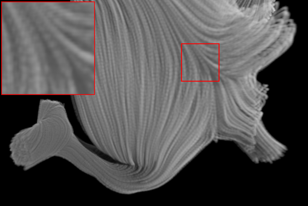
(b) SDF occupancy without clipping planes

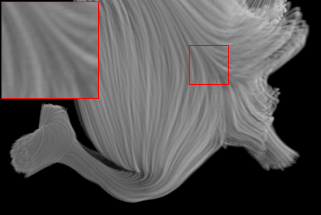
(c) SDF occupancy with clipping planes

Figure 4: Volume renderings of the occupancy pyramid of the Aneurysm line set. Without clipping, spherical artifacts appear at every interior vertex. When using the clipped capsule SDF, artifacts are resolved and aliasing is significantly reduced compared to DDA voxelization.

(a) DDA occupancy

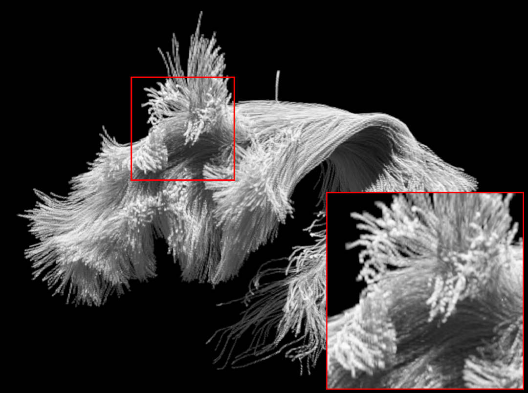
(b) SDF occupancy without PWAA

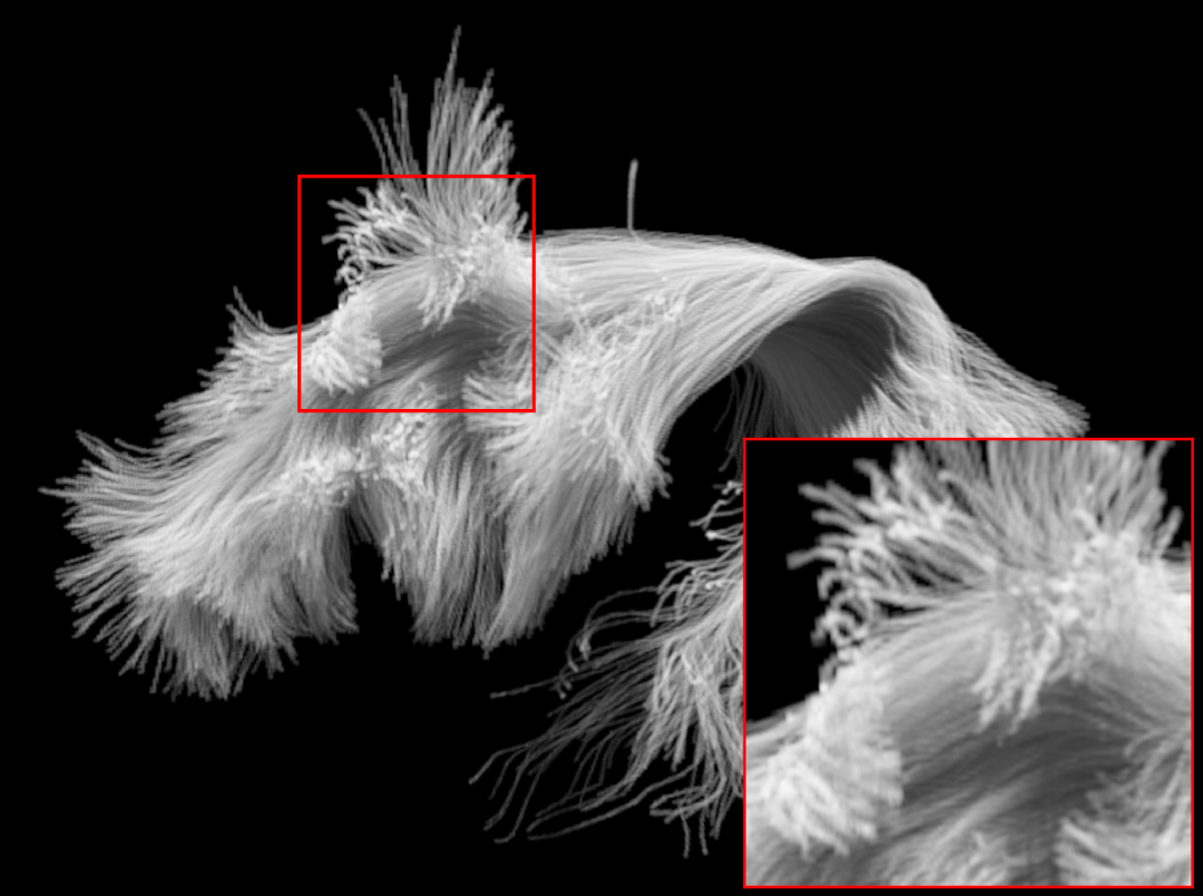
(c) SDF occupancy with PWAA

Figure 5: Volume renderings of the occupancy pyramid of the Arcuate Fasciculus line set. Without Phone-Wire Anti-Aliasing, thin lines introduce aliasing and an overestimation of total occupancy. With Phone-Wire Anti-Aliasing these artifacts are reduced.

To further investigate the voxelization performance of the three voxelization strategies, we evaluated the relation between performance and line segment length, which is shown in Figure 6. To evaluate this relation, we computed various levels of detail of the high resolution Whole Brain 1M dataset by linking every $n$th vertex to produce level of detail $n$. This resulted in datasets that span more or less the same number of voxels but have increasing average line segment lengths. For all tests, voxelization performance was measured using a resolution of $256^{3}$ and a line radius of $0.2$.

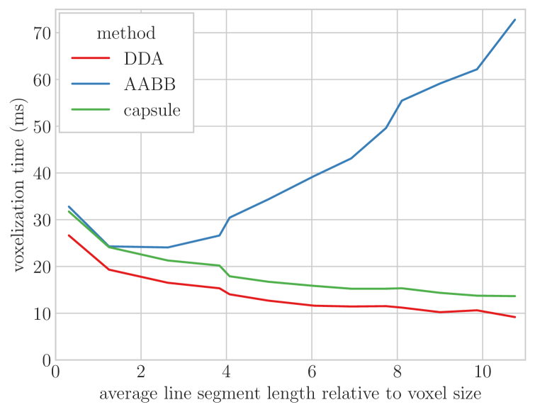
Figure 6: Voxelization performance as a function of segment length

Figure 6 clearly demonstrates the effectiveness of the proposed capsule voxelization algorithm compared to the AABB approach when voxelizing longer line segments. Capsule voxelization adds a fixed overhead compared to DDA voxelization. These findings corroborate the theorized efficiencies in Section 3.1.

Now that we have investigated the performance of three voxelization strategies, we turn our attention to the qualitative aspects of voxelization. Since DDA only visits voxels that are directly intersected by the zero-radius line segment, occupancy estimation is restricted to those voxels, leading to aliasing at larger line radii. Conservative voxelization visit all voxels that are intersected by the capsule primitive, allowing for better occupancy estimation. We will evaluate how clipping planes and Phone-Wire Anti-Aliasing improve the SDF-based occupancy estimation compared to DDA.

Figure 4 shows a comparison between DDA-based occupancy and SDF-based occupancy with and without clipping planes. The DDA-based occupancy, shown in Figure fig.˜4(a) clearly exhibits aliasing for larger line radii. When using SDF-based occupancy without clipping planes, shown Figure fig.˜4(b), aliasing is reduced, but spherical artifacts appear at every interior vertex. This leads to occupancy overestimation, especially when voxelizing short segments with relatively large radii. By using our clipped capsule signed distance function, shown in Figure fig.˜4(c), the spherical artifacts are removed and aliasing is reduced compared to DDA.

Figure 5 shows a comparison between DDA-based occupancy and SDF-based occupancy with and without Phone-Wire Anti-Aliasing (PWAA). As can be seen in Figure fig.˜5(a), DDA-based occupancy estimation produces only minimal aliasing for thin line segments. However, SDF-based occupancy without PWAA, shown in Figure fig.˜5(b), introduces severe aliasing, resulting in an overestimation of occupancy. The aliasing is removed when using PWAA, shown in Figure fig.˜5(c), and shows similar if not slightly reduced aliasing compared to DDA-based occupancy.

Figure 7 clearly demonstrates the need for conservative voxelization to remove missing-segment artifacts during ray-tracing, which happen when a ray passes through a voxel which is not aware of a primitive being in that voxel. These artifacts manifest themselves as cubical cutouts and become more apparent with larger line radii relative to voxel size. When using a conservative voxelization scheme, these artifacts are completely resolved.

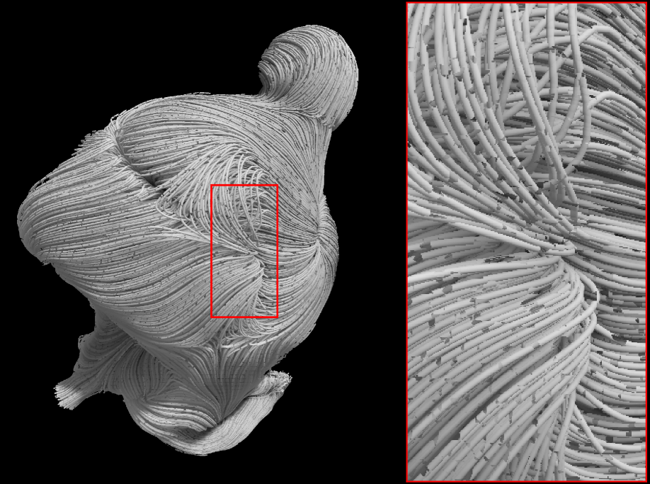
(a) Non-Conservative Voxelization

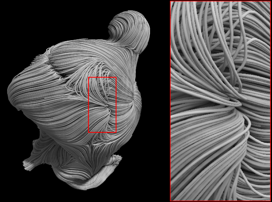
(b) Conservative Voxelization

Figure 7: Comparison of ray-tracing using conservative versus non-conservative voxelization for the Aneurysm dataset. Cube-like artifacts are visible when employing non-conservative voxelization. Conservative voxelization correctly renders the capsule primitives.

To conclude, these results show that the choice of voxelization algorithm depends on the voxelization scenario. DDA voxelization has the best performance and shows minimal aliasing for thin line segments, but is not conservative. When used as the basis for ray tracing or when voxelizing thicker line segments, conservative voxelization should be used. As theorized, capsule voxelization scales better with segment length, having linear time complexity, compared to the worst case cubic complexity of AABB voxelization.

4.2 A-Buffer

Our A-Buffer approach is based on the Linearized Layered Fragment Buffer [KLZ12], where all fragments are captured using a two pass voxelization scheme: voxelize-scan-voxelize (VSV). To improve performance for (semi-)opaque datasets, we introduced a view-dependent culling step to speed up the secondary voxelization pass: voxelize-cull-scan-voxelize (VCSV). In this section, we will compare these two approaches to another common approach in literature: voxelize-sort-scan (VSS) [KRW18, McG20], using OneSweep [AM22] as a fast sorting implementation. In Table 3 we compare these strategies to compute both the occupancy pyramid and the A-Buffer, i.e. all per-frame preprocessing required to enable dynamic ray tracing and ambient occlusion.

Dataset	VSS	VSV (ours)	VCSV (ours)
Bundles Small	14	5	4
Aneurysm	21	6	4
Bundles Large	75	18	12
Brain 200k	67	20	12
Turbulence	120	46	21
Brain 1M	1015	104	50

Table 3: Performance in milliseconds to produce both the occupancy pyramid and the A-Buffer at a resolution of $128^{3}$ for: voxelize-sort-scan (VSS), voxelize-scan-voxelize (VSV) and voxelize-cull-scan-voxelize (VCSV) for opaque geometry.

As expected, voxelize-scan-voxelize (VSV) performs better than voxelize-sort-scan (VSS) while producing the same A-Buffer and occupancy pyramid. The threefold speedup aligns with the theoretical advantage of the VSV, needing only two passes over all fragments and one scan over all voxels, while voxelize-sort-scan needs 7 passes (one write, five for sorting, one for scanning all fragments). While the morton-order sorting generates a cache efficient acceleration structure, the same can be achieved by the choice of scan pass in the voxelize-scan-voxelize strategy.

Another advantage of the voxelize-scan-voxelize (VSV) strategy is the potential of accelerating the secondary voxelization pass. The occupancy pyramid generated in the primary voxelization pass enables view-dependent culling of the secondary voxelization pass, creating a partial A-Buffer. Comparing this strategey, voxelize-cull-scan-voxelize (VCSV), with voxelize-scan-voxelize (VSV) when rendering opaque geometry, we can see a performance gain up to two times. This performance gain depends on line set density and the chosen camera angle. Altogether, our method cuts down per-frame preprocessing time by a factor of 3 when rendering transparent data (VSV) or a factor of 6 for dynamic opaque data.

4.3 Rendering

Next, we compare our dynamic rendering pipeline to the state of the art by evaluating the performance of our method against the method of Kanzler et al. [KRW18] and Groß and Gumhold [GG20], who both render line sets with ambient occlusion and transparency. We test the dynamic aspect of our method and the state of the art by including all per-frame preprocessing costs in all performance measurements. By building all acceleration structures from scratch every frame, all rendering pipelines can handle any potential dynamic behavior. Since the state of the art relies on a fast sorting algorithm, we used the OneSweep radix sort algorithm [AM22].

Groß and Gumholds rasterization method [GG20] can handle dynamic data, except for the construction of the occupancy pyramid. Therefore we used fast DDA voxelization to generate the occupancy pyramid every frame, making their method fully dynamic. Otherwise all aspects are kept the same as in the original paper.

We used the GPU quantization method of Kanzler et al. [KRW18] to construct the A-Buffer and occupancy pyramid every frame, making their method fully dynamic. We use a quantization resolution of $64^{2}$, which makes each segment fit in 32 bits for optimal performance. While the original paper includes a level of detail system, we decided to omit it in our experiments because such a system could be implemented for both Groß and Gumhold and our method. Because it reduces performance significantly, we exclude the author’s proposed voxel neighborhood sampling for both performance and quality evaluation.

As a performance reference, we additionally compare these methods to a Baseline opaque rasterization using a Z-Buffer, implemented as Groß and Gumholds method [GG20] without sorting and culling and using DDA to compute the occupancy pyramid.

All experiments target a screen resolution of $1920\times 1080$ and measure the time it takes to complete the entire dynamic rendering pipeline with ambient occlusion, assuming a full recompute of the acceleration structures every frame for every method. A voxel resolution of $128^{3}$ was chosen, since it gives optimal ray tracing performance according to our experiments and does not affect line rendering quality for our method. A line radius of 0.2 times the voxel size was chosen.

Table 4 shows the rendering performance when rendering dynamic opaque geometry. When rendering dynamic opaque line sets, our method performs best across all line sets. Our method is closely followed by Kanzler et al., but at the cost of quantization and missing-segment artifacts. Our performance gains are attributable to our proposed A-Buffer and culling method, which is especially effective when rendering opaque lne sets. Compared to the rasterization techniques (Baseline and Groß), the ray-tracing techniques (Kanzler and Ours) have the advantage of early ray termination and show superior performance on larger line sets. As expected, all methods perform better than Baseline rasterization.

Dataset	Baseline	Groß	Kanzler	Ours
Bundles Small	13	12	13	10
Aneurysm	25	20	13	9
Bundles Large	83	44	39	22
Brain 200k	138	81	30	28
Turbulence	209	127	47	41
Brain 1M	822	417	119	117

Table 4: Opaque rendering performance in milliseconds, including per-frame preprocessing costs.

Dataset	Groß	Kanzler	Ours
Bundles Small	32	35	54
Aneurysm	39	30	55
Bundles Large	81	67	89
Brain 200k	127	55	117
Turbulence	175	97	199
Brain 1M	596	158	276

Table 5: Transparent rendering performance in milliseconds at an opacity of 0.1, including all per-frame preprocessing costs.

Table 5 shows the rendering performance when rendering transparent geometry using an opacity of 0.1. When rendering transparent geometry, Kanzler et al. shows the best performance for most datasets. While our method is fast when rendering opaque data, performance is significantly reduced when rendering full transparency. This is to be expected, since the conservative voxelization increases the number of fragments and therefore ray-capsule intersection tests, which dominate the rendering time when rendering full transparency. Kanzler et al.’s quantized method increases performance by limiting the amount of ray-capsule intersections compared to more accurate methods.

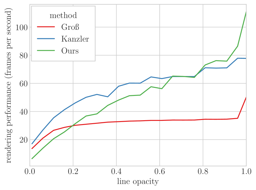
Figure 8: Performance (frames per second, including per-frame preprocessing) when rendering Aneurysm at various line opacities.

To further investigate the impact of line opacity on dynamic rendering performance, we evaluated rendering the Aneurysm line set at various opacity values, shown in Figure 8. This figure clearly shows the benefit of early ray-termination when using a ray tracing approach, compared with the hierarchical culling strategy of Groß and Gumhold. Given that our method renders correct transparency without any quantization and artifacts, it performs quite well compared to the method of Kanzler et al., even showing superior performance for very high line opacities.

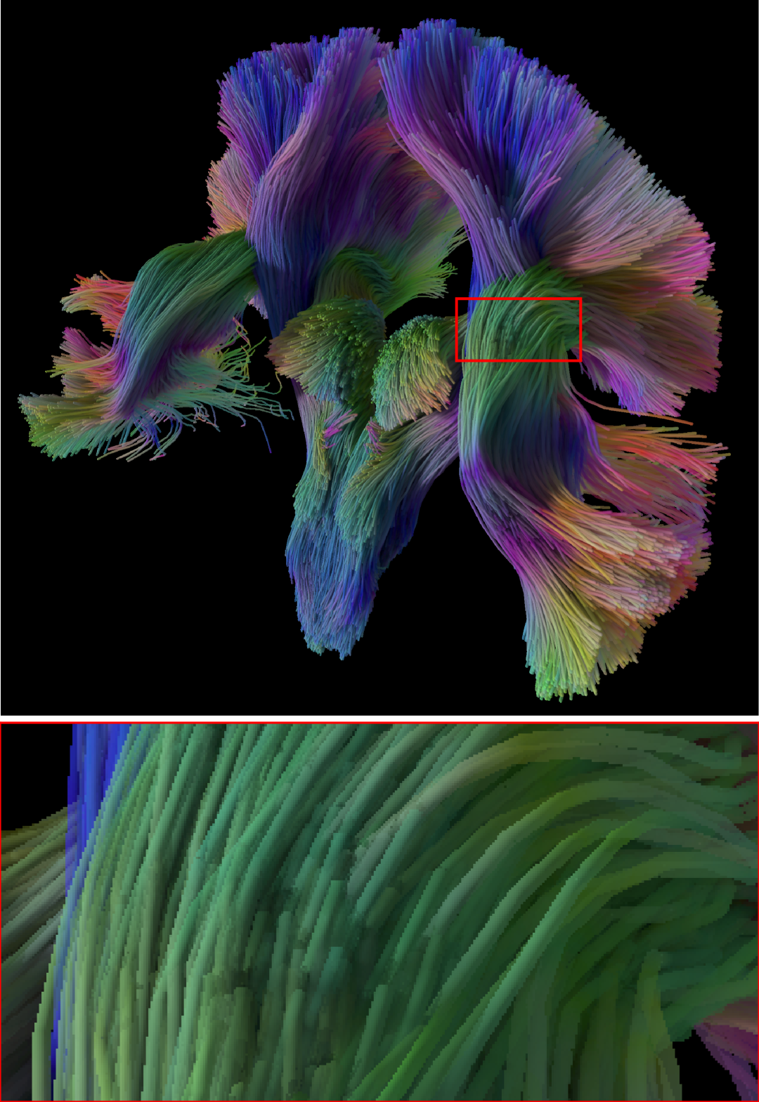
(a) Groß and Gumhold

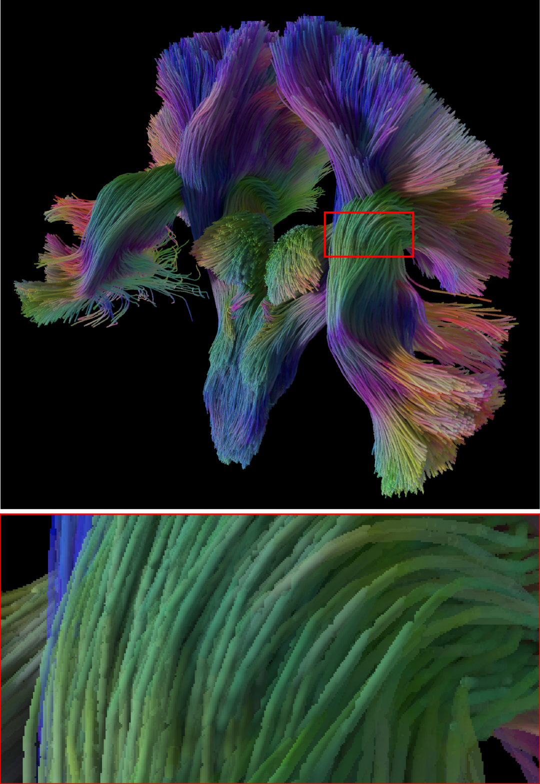
(b) Kanzler et al.

(c) Ours

Figure 9: Qualitative comparison between rendering methods.

Finally, we compare rendering quality with the state of the art by comparing semi-opaque renderings of the Bundles Small line set, shown in Figure 9, which presents a challenge for the state of the art. While all methods achieve very similar overall renderings due to the use of identical shading and tangent-coloring, looking closer reveals qualitative differences. While their method works very well for shorter line segments, Groß and Gumhold’s K-Buffer-based order correcting algorithm fails to properly sort the relatively long line segments in this dense tractogram. Being non-conservative, Kanzler et al.’s method shows missing-segment artifacts, which reduces the quality of the rendered lines, but is less noticeable when rendering full transparency. Our voxel-based ray tracing guarantees correct ordering and resolves missing-segment artifacts.

5 Conclusion and Future Work

We have presented a real-time rendering pipeline for voxel-based ray-tracing of dynamic line sets, including ambient occlusion and correct transparency. We increased rendering performance by introducing a conservative capsule voxelization method and a voxel-based culling approach to efficiently compute the A-Buffer.

A limitation of our approach is the low rendering performance when rendering lines at low opacity values, which may be resolved by incorporating a level of detail approach.

For future work, we will investigate whether rendering performance can be improved further by incorporating level of detail rendering, possibly using volume rendering, or making use of frame coherence. Finally, we will investigate how interactive tractography segmentation techniques can benefit from this rendering approach.

Appendix A Line Set Renderings

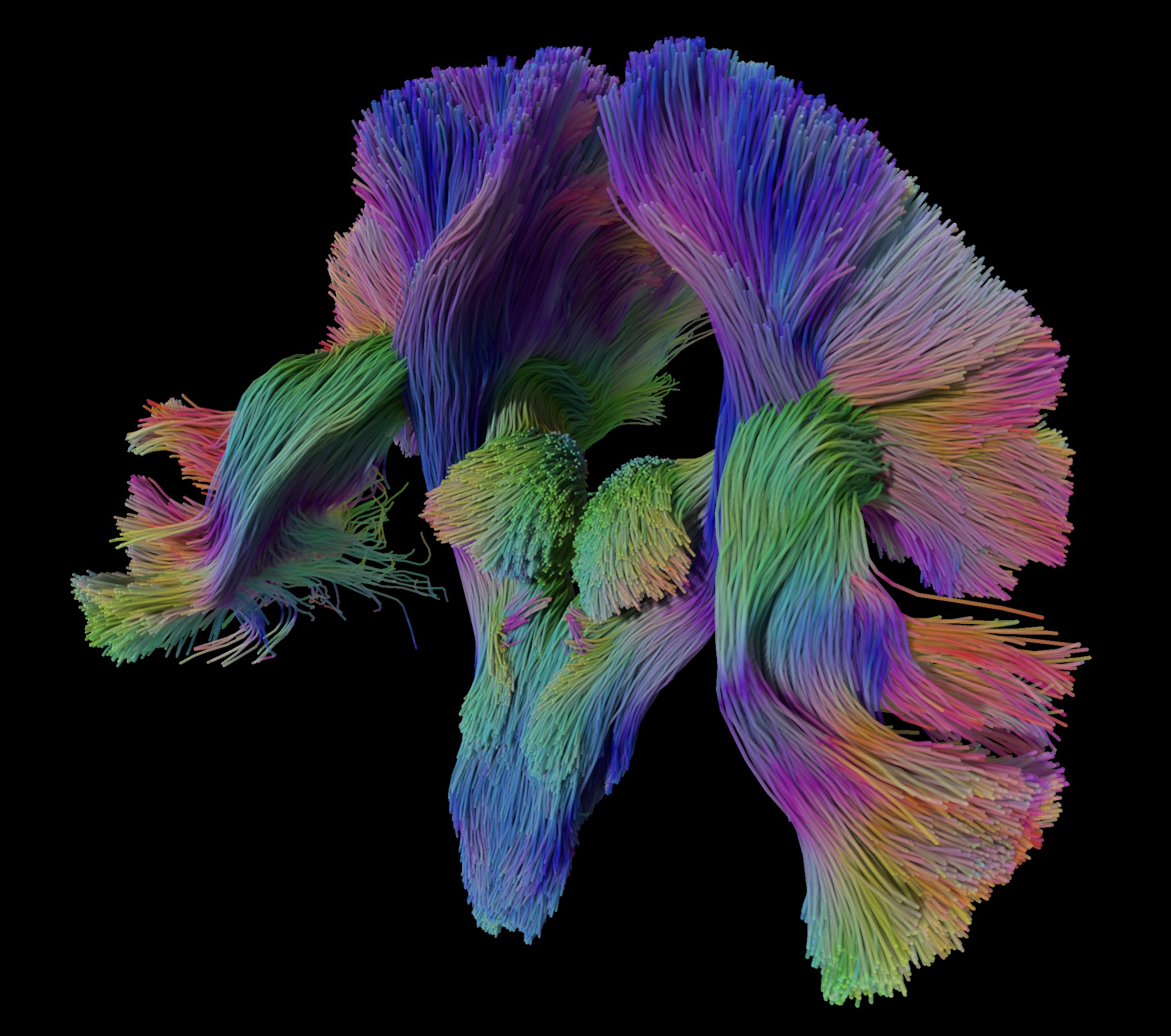
(a) Bundles Small

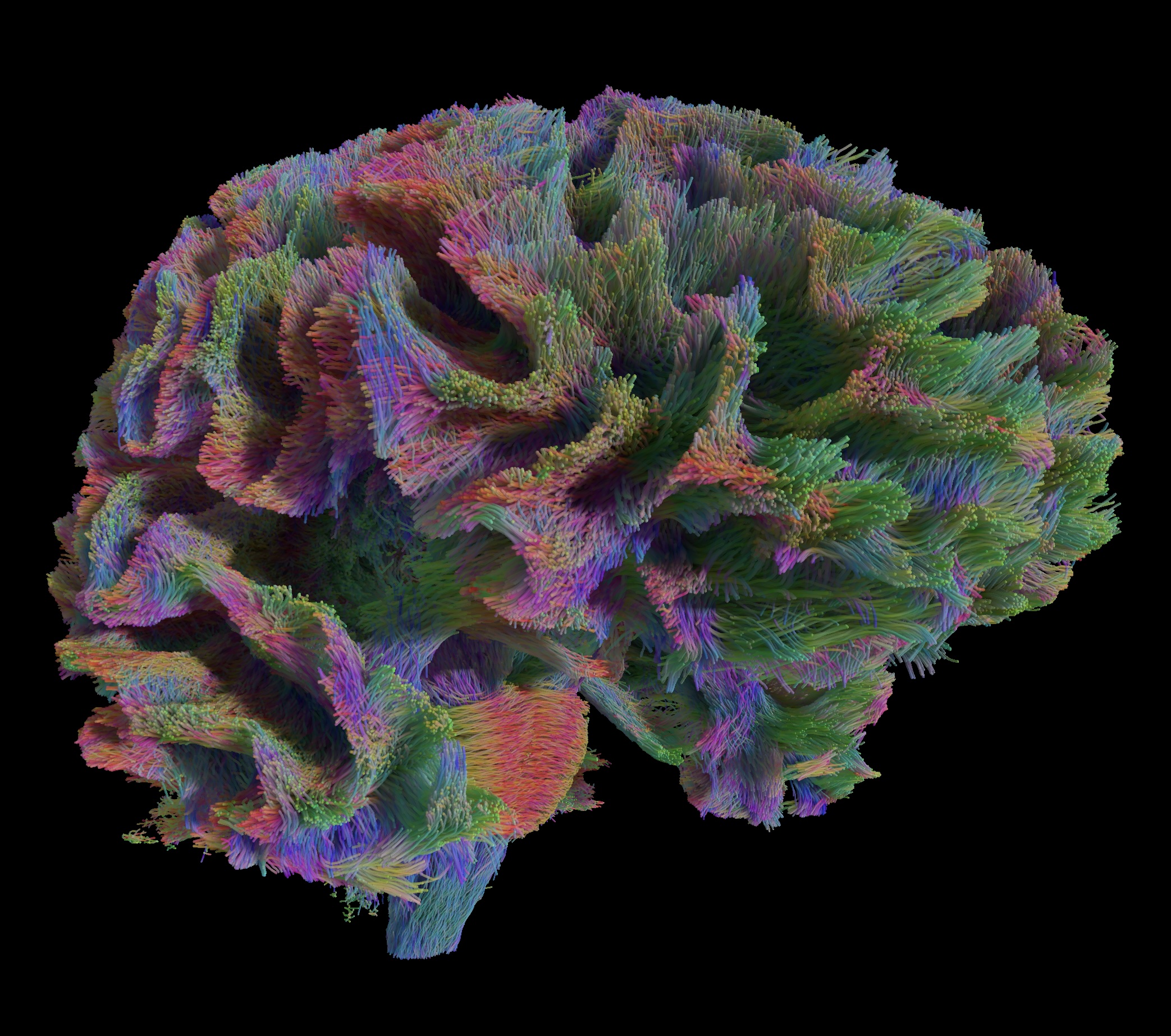
(b) Brain 200k

(c) Aneurysm

(d) Bundles Large

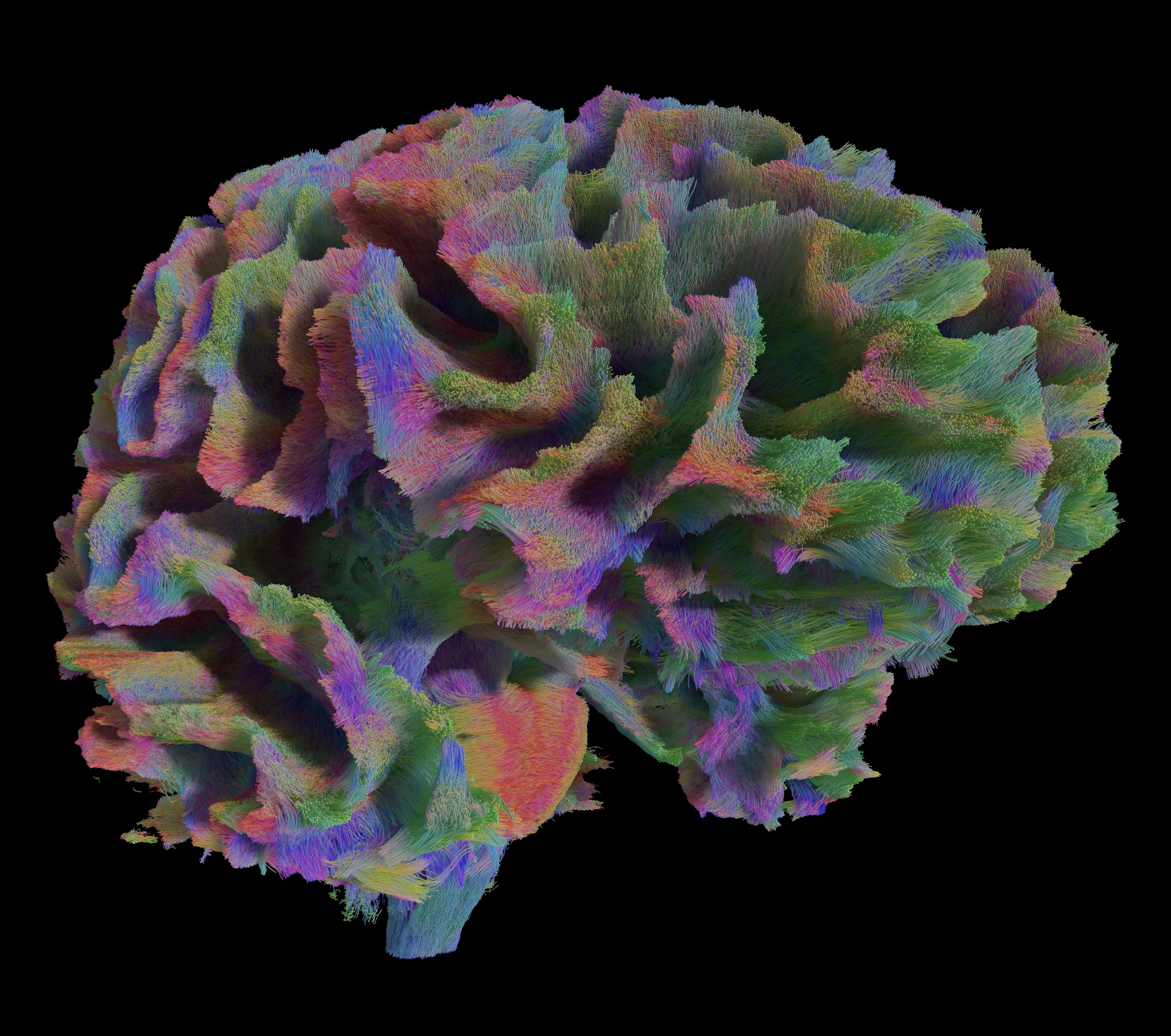
(e) Brain 1M

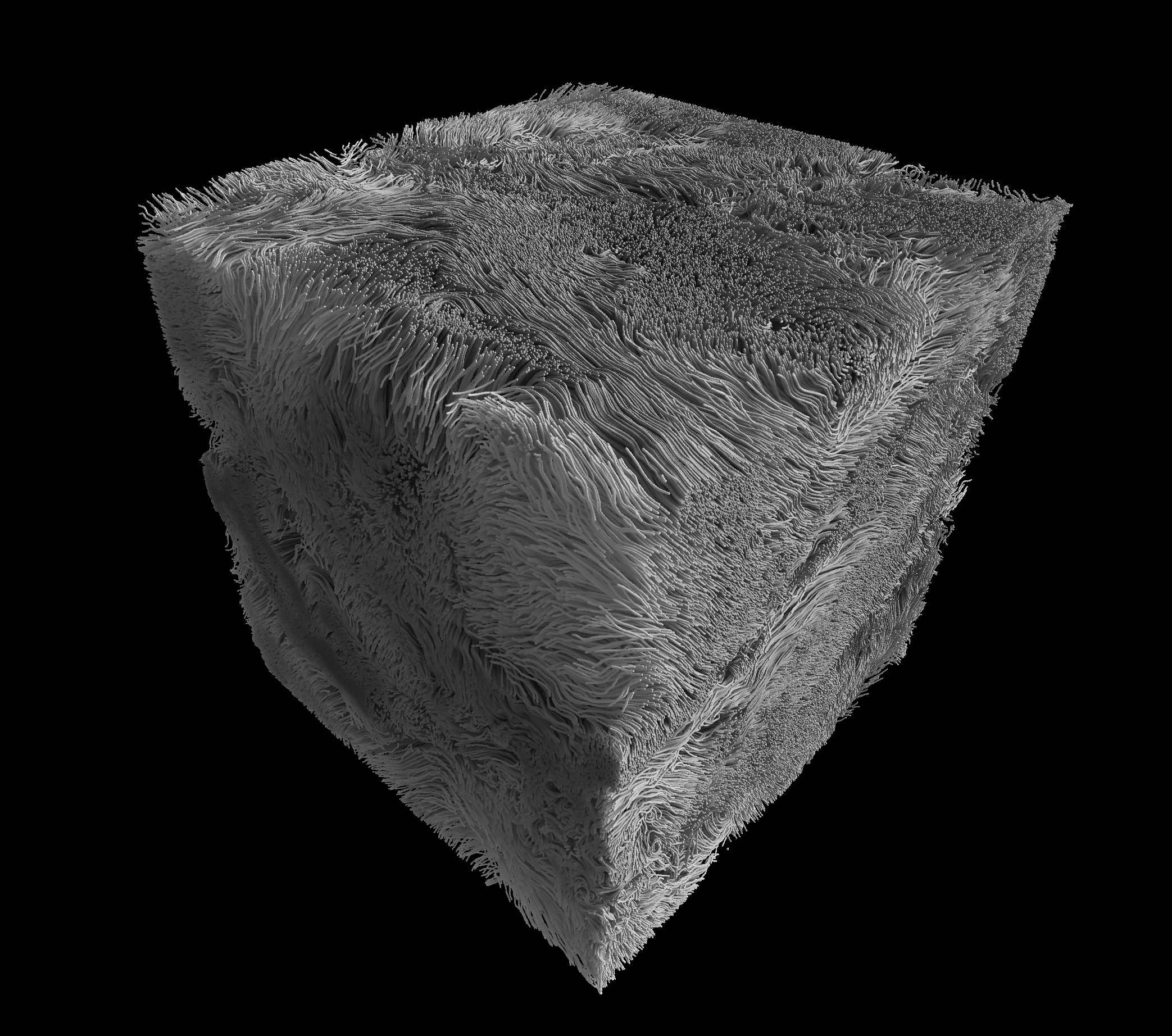
(f) Turbulence

References

- [AM22] Adinets A., Merrill D.: Onesweep: A faster least significant digit radix sort for gpus. arXiv preprint arXiv:2206.01784 (2022).
- [ASH∗09] Anwander A., Schurade R., Hlawitschka M., Scheuermann G., Knösche T. R.: White matter imaging with virtual klingler dissection. NeuroImage 47 (2009), S105.
- [AW∗87] Amanatides J., Woo A., et al.: A fast voxel traversal algorithm for ray tracing. In Eurographics (1987), vol. 87, pp. 3–10.
- [BCL∗07] Bavoil L., Callahan S. P., Lefohn A., Comba J. L., Silva C. T.: Multi-fragment effects on the gpu using the k-buffer. In Proceedings of the 2007 symposium on Interactive 3D graphics and games (2007), pp. 97–104.
- [Bre65] Bresenham J.: Algorithm for computer control of a digital plotter. IBM SYSTEMS JOURNAL 4, 1 (1965), 25.
- [Car84] Carpenter L.: The a-buffer, an antialiased hidden surface method. In Proceedings of the 11th annual conference on Computer graphics and interactive techniques (1984), pp. 103–108.
- [CNS∗11] Crassin C., Neyret F., Sainz M., Green S., Eisemann E.: Interactive indirect illumination using voxel cone tracing. In Computer Graphics Forum (2011), vol. 30, Wiley Online Library, pp. 1921–1930.
- [Cra10] Crassin C.: Opengl 4.0+ abuffer v2.0: Linked lists of fragment pages, 2010. URL: https://blog.icare3d.org/2010/07/opengl-40-abuffer-v20-linked-lists-of.html.
- [CWF∗14] Chamberland M., Whittingstall K., Fortin D., Mathieu D., Descoteaux M.: Real-time multi-peak tractography for instantaneous connectivity display. Frontiers in neuroinformatics 8 (2014), 59.
- [DRN∗17] Díaz J., Ropinski T., Navazo I., Gobbetti E., Vázquez P.-P.: An experimental study on the effects of shading in 3d perception of volumetric models. The visual computer 33, 1 (2017), 47–61.
- [EHS12] Eichelbaum S., Hlawitschka M., Scheuermann G.: Lineao—improved three-dimensional line rendering. IEEE Transactions on Visualization and Computer Graphics 19, 3 (2012), 433–445.
- [Eve01] Everitt C.: Interactive order-independent transparency. White paper, nVIDIA 2, 6 (2001), 7.
- [GG20] Groß D., Gumhold S.: Advanced rendering of line data with ambient occlusion and transparency. IEEE Transactions on Visualization and Computer Graphics 27, 2 (2020), 614–624.
- [GRDE10] Grottel S., Reina G., Dachsbacher C., Ertl T.: Coherent culling and shading for large molecular dynamics visualization. In Computer Graphics Forum (2010), vol. 29, Wiley Online Library, pp. 953–962.
- [HCTS10] Hsieh H.-H., Chang C.-C., Tai W.-K., Shen H.-W.: Novel geometrical voxelization approach with application to streamlines. Journal of Computer Science and Technology 25, 5 (2010), 895–904.
- [HG12] Harris M., Garland M.: Optimizing parallel prefix operations for the fermi architecture. In GPU Computing Gems Jade Edition. Elsevier, 2012, pp. 29–38.
- [HGVV16] Hermosilla P., Guallar V., Vinacua A., Vázquez P.-P.: High quality illustrative effects for molecular rendering. Computers & Graphics 54 (2016), 113–120.
- [Ker20] Kern M.: Large 3d line sets for opacity-based rendering, Feb 2020. URL: https://zenodo.org/records/3637625.
- [KLZ12] Knowles P., Leach G., Zambetta F.: Efficient layered fragment buffer techniques 20. OpenGL Insights (2012), 279.
- [KNM∗20] Kern M., Neuhauser C., Maack T., Han M., Usher W., Westermann R.: A comparison of rendering techniques for 3d line sets with transparency. IEEE Transactions on Visualization and Computer Graphics 27, 8 (2020), 3361–3376.
- [KRW18] Kanzler M., Rautenhaus M., Westermann R.: A voxel-based rendering pipeline for large 3d line sets. IEEE transactions on visualization and computer graphics 25, 7 (2018), 2378–2391.
- [McG20] McGraw T.: High-quality real-time raycasting and raytracing of streamtubes with sparse voxel octrees. In 2020 IEEE Visualization Conference (VIS) (2020), IEEE, pp. 21–25.
- [MLP∗10] McLoughlin T., Laramee R. S., Peikert R., Post F. H., Chen M.: Over two decades of integration-based, geometric flow visualization. In Computer Graphics Forum (2010), vol. 29, Wiley Online Library, pp. 1807–1829.
- [Per12] Person E.: Phone-wire aa, 2012. URL: https://www.humus.name/index.php?page=3D&ID=89.
- [Qui08] Quilez I.: Distance functions, 2008. Accessed: 2025‑07‑30. URL: https://iquilezles.org/articles/distfunctions/.
- [Qui13] Quilez I.: Intersectors, 2013. Accessed: 2025-07-30. URL: https://iquilezles.org/articles/intersectors/.
- [SGG15] Staib J., Grottel S., Gumhold S.: Visualization of particle-based data with transparency and ambient occlusion. In Computer Graphics Forum (2015), vol. 34, Wiley Online Library, pp. 151–160.
- [SM04] Schussman G., Ma K.-L.: Anisotropic volume rendering for extremely dense, thin line data. In IEEE Visualization 2004 (2004), IEEE, pp. 107–114.
- [SSA∗08] Schultz T., Sauber N., Anwander A., Theisel H., Seidel H.-P.: Virtual klingler dissection: Putting fibers into context. In Computer Graphics Forum (2008), vol. 27, Wiley Online Library, pp. 1063–1070.
- [TSR∗19] Tournier J.-D., Smith R., Raffelt D., Tabbara R., Dhollander T., Pietsch M., Christiaens D., Jeurissen B., Yeh C.-H., Connelly A.: Mrtrix3: A fast, flexible and open software framework for medical image processing and visualisation. Neuroimage 202 (2019), 116137.
- [VESB∗13] Van Essen D. C., Smith S. M., Barch D. M., Behrens T. E., Yacoub E., Ugurbil K., Consortium W.-M. H., et al.: The wu-minn human connectome project: an overview. Neuroimage 80 (2013), 62–79.
- [WBK∗07] Ward K., Bertails F., Kim T.-Y., Marschner S. R., Cani M.-P., Lin M. C.: A survey on hair modeling: Styling, simulation, and rendering. IEEE transactions on visualization and computer graphics 13, 2 (2007), 213–234.
- [WMZ∗20] Wald I., Morrical N., Zellmann S., Ma L., Usher W., Huang T., Pascucci V.: Using hardware ray transforms to accelerate ray/primitive intersections for long, thin primitive types. Proceedings of the ACM on Computer Graphics and Interactive Techniques 3, 2 (2020), 1–16.
- [WNMH18] Wasserthal J., Neher P., Maier-Hein K. H.: Tractseg-fast and accurate white matter tract segmentation. Neuroimage 183 (2018), 239–253.
- [Wu91] Wu X.: An efficient antialiasing technique. Acm Siggraph Computer Graphics 25, 4 (1991), 143–152.
- [YHGT10] Yang J. C., Hensley J., Grün H., Thibieroz N.: Real-time concurrent linked list construction on the gpu. In Computer Graphics Forum (2010), vol. 29, Wiley Online Library, pp. 1297–1304.