MCMC: Bridging Rendering, Optimization, and Generative AI

Gurprit Singh¹, Wenzel Jakob^2
1Max Planck Institute for Informatics, Germany, ²EPFL, Switzerland
SIGGRAPH Asia 2024 Course notes

Abstract.

Generative artificial intelligence (AI) has made unprecedented advances in vision language models over the past two years. These advances are largely due to diffusion-based generative models, which are very stable and simple to train. These diffusion models are tasked to learn the underlying unknown distribution of the training data samples. During the generative process, new samples (images) are generated from this unknown high-dimensional distribution. Markov Chain Monte Carlo (MCMC) methods are particularly effective in drawing samples from complex, high-dimensional distributions. This makes MCMC methods an integral component for both the training and sampling phases of these models, ensuring accurate sample generation.

Gradient-based optimization is at the core of modern generative models. The update step during the optimization forms a Markov chain where the new update depends only on the current state. This allows exploration of the parameter space in a memoryless manner, thus combining the benefits of gradient-based optimization and MCMC sampling. MCMC methods have shown an equally important role in physically based rendering where complex light paths are otherwise quite challenging to sample from simple importance sampling techniques.

A lot of research is dedicated towards bringing physical realism to samples (images) generated from diffusion-based generative models in a data-driven manner, however, a unified framework connecting these techniques is still missing. In this course, we take the first steps toward understanding each of these components and exploring how MCMC could potentially serve as a bridge, linking these closely related areas of research. Our course aims to provide necessary theoretical and practical tools to guide students, researchers and practitioners towards the common goal of generative physically based rendering. All Jupyter notebooks with demonstrations associated to this tutorial can be found on our project webpage https://sinbag.github.io/mcmc/.

Contents

1. 1 Overview
2. 2 Theoretical background
   1. 2.1 Stochastic differential equations (SDEs)
      1. 2.1.1 Brownian motion
      2. 2.1.2 Langevin Dynamics
      3. 2.1.3 Hamiltonian Dynamics
   2. 2.2 Monte Carlo integration
   3. 2.3 MCMC sampling methods
      1. 2.3.1 Metropolis-Hastings algorithm
      2. 2.3.2 Langevin Monte Carlo sampling
      3. 2.3.3 Annealed Langevin Monte Carlo sampling
      4. 2.3.4 Hamiltonian Monte Carlo sampling
      5. 2.3.5 Discussion
3. 3 MCMC in rendering
   1. 3.1 Path-space
   2. 3.2 Multiple Importance Sampling
   3. 3.3 Limitations of Monte Carlo Path Sampling
   4. 3.4 Metropolis Light Transport
   5. 3.5 Primary sample space MLT
   6. 3.6 Hessian-Hamiltonian MLT
4. 4 MCMC in optimization
   1. 4.1 Bayesian inference
   2. 4.2 Stochastic gradient descent (SGD)
   3. 4.3 Stochastic Gradient Langevin Dynamics (SGLD)
   4. 4.4 Bayesian inference using SGD
5. 5 MCMC in generative modeling
   1. 5.1 From variatonal autoencoders to variational diffusion models
      1. 5.1.1 Evidence lower bound (ELBO).
      2. 5.1.2 Variational autoencoders (VAEs).
      3. 5.1.3 Hiearchical VAEs (HVAEs).
      4. 5.1.4 Variational diffusion models.
   2. 5.2 Energy-based models (EBM)
      1. 5.2.1 MCMC methods for sampling from EBMs
   3. 5.3 Sampling score-based generative models
6. 6 Conclusion
7. 7 Speakers
8. A Code snippets

1 Overview

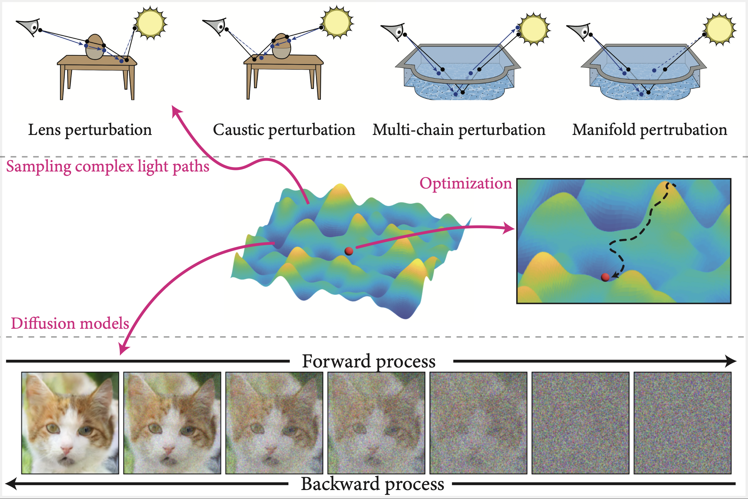
Figure 1: This course provides an overview of MCMC methods, which are powerful tools for sampling from complex distributions. An example of such a distribution is shown in the middle row (Part II). These complex distributions are common in physically based rendering and generative modeling. Additionally, we will review the impact of MCMC methods on gradient-based optimization techniques, which typically aim to find good local (or global) minima in the optimization landscape (inset on the middle-right).

MCMC methods are powerful tools for sampling from complex, high-dimensional probability distributions, which are ubiquitous in modern computational problems. Whether you are working with Bayesian inference in statistics, machine learning, or any field involving probabilistic models, MCMC provides a robust framework for gaining insights and making accurate predictions.

In this course, we introduce the terminology associated to probabilistic models. We start from the theoretical foundations essential to establish the ground work for Markov chains Section˜2. We introduce stochastic differential equations (SDEs) that are essential to describe stochastic systems evolving over time. Brownian motion is one such example. We later on discuss Langevein and Hamiltonian dynamics which are capable of exploring the anisotropic regions far more efficiently. Markov chains are a memoryless way to sample paths described by the SDEs. In Section˜3, we discuss various Markov chain Monte Carlo (MCMC) sampling methods with direct applications to physically based rendering. In Section˜4, we introduce stochastic gradient descent (SGD) optimization algorithm which is at the core of all machine learning tasks. We show that SGD update step can be seen as a Markov chain and more advanced MCMC sampling methods can be employed to better explore the optimization manifolds. Lastly, in LABEL:mcmc_generative we study variational autoencoders, how they are driven by evidence lower bound and their connection to variational diffusion models. We then discuss energy-based models which, although slow to train, provides a lot of flexibility. We conclude with the exciting research directions that can follow from this course.

2 Theoretical background

Markov Chains are mathematical models used to describe systems that transition from one state to another, where the probability of each transition depends only on the current state (this property is known as the "memoryless" property or Markov property). The system moves between discrete states with given transition probabilities. Markov Chains are often represented as sequences of random variables.

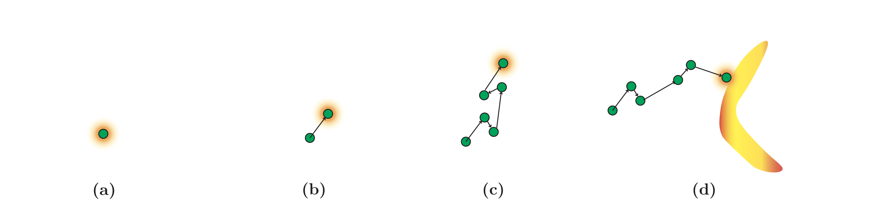
Figure 2: To create a Markov chain, we start with a random sample (a) that is generated with a given proposal (shown in orange). (b) This sample becomes the current state. The next sample (new state) is then generated from the current state following the proposal. (c) As the chain continues to grow, we obtain a sequence of samples that represents a Markov chain. (d) When run long enough, this Markov chain can generate samples that matches the target distribution.

2.1 Stochastic differential equations (SDEs)

SDEs describe systems that evolve over continuous time with randomness (noise) involved. SDEs often model complex phenomena like stock prices or physical systems influenced by random factors. It describes how we simulate motion numerically. The motion could be of organic "microscopic" particles or of inorganic particles.

Consider particles jiggling in the water (shown on the right). There are a huge number of water molecules ($\sim 10^{24}$). Each particle is on average moving along certain trajectory (i.e., drift) with some jiggle (randomness or diffusion). SDEs can be used to simulate such stochastic motion. Even though the particles are jiggling in random directions, in ensemble, their motion can be well-predicted. An SDE typically takes the form [Roberts and Stramer, 2002]:

$$d\mathbf{x}_{t}=\underbrace{\mu(\mathbf{x}_{t},t)}_{\text{drift}}dt+\underbrace{\sigma(\mathbf{x}_{t},t)}_{\text{rate of diffusion}}\!\!\!\!\!\!dW_{t}$$ (1)

where $\mathbf{x}_{t}$ is the state variable at time $t$, $\mu(\mathbf{x}_{t},t)$ is the drift term, representing the deterministic part of the dynamics, $\sigma(\mathbf{x}_{t},t)$ is the diffusion term, representing the stochastic part of the dynamics and $W_{t}$ is a Wiener process or Brownian motion, which introduces randomness into the system.

The solution of an SDE can exhibit the Markov property, where future behavior depends only on the present state and not on the path that led to it. In continuous time, the evolution of states in an SDE can be thought of as a continuous Markov process.

2.1.1 Brownian motion

Brownian motion is the simplest form of an SDE and serves as the foundation for more complex models (like Langevin dynamics). It is also known as a Wiener process. It is a continuous-time stochastic process with the following properties:

• $W_{0}=x_{0}$.

• $W_{t_{1}}$ has independent increments.

• $W_{t_{2}}-W_{t_{1}}\sim\mathcal{N}(0,t-s)$ for $0\leq t_{1}<t_{2}$.

• $W_{t}$ varies continuously wrt to $t$.

It is a fundamental stochastic process that describes the random motion of particles suspended in a fluid. The motion is typically modeled as a stochastic process or random walk. The motion is completely random with no memory of past states, and it’s often modeled using the Fokker-Planck equation for probability density evolution or as a pure diffusion process. It is used to describe motion at very small scales (e.g., molecular scales) where thermal fluctuations dominate. In Fig.˜3, we simulate the random walk in space. Although the motion is fully stochastic, it can be directed to follow certain constraints.

(a)	(b)	(c)	(d)	(e)

Figure 3: Brownian motion for different target densities. Simulating Brownian motion is the same as performing a random walk (a). However, we can restrict the motion along certain trajectories (b-e). The red dot represents the starting point, and the blue dashed line (b,d) or the blue region (c) represents the targetted region/trajectory. The motion is simulated to partially fill the space to demonstrate the evolution of the Markov chain.

2.1.2 Langevin Dynamics

Langevin dynamics describes the motion of a particle under the influence of both deterministic forces and random noise. It extends Brownian motion by adding a drift term representing deterministic forces and a damping term. It models systems where particles experience both random thermal fluctuations and deterministic forces. The Langevin equation is an SDE and is given by

$$\lambda\frac{d\mathbf{x}_{t}}{dt}=-\frac{dU(\mathbf{x})}{d\mathbf{x}}+\eta(\mathbf{x})$$ (2)

where $U(x)$ is the potential energy as a particle’s position $\mathbf{x}_{t}$ and $\eta(x)$ is the noise term. The potential energy term represents the influence of an external or internal force that depends on the particle’s position and is typically associated with physical interactions like gravity, electrostatic forces, or molecular bonds. The dynamics of the Langevin equation Eq.˜2 can be written as:

$$d\mathbf{x}_{t}=-\nabla U(\mathbf{x})dt+\sqrt{2}\;dW_{t}$$ (3)

where $dW_{t}$ represents the time derivation of the standard Brownian motion. The potential energy term guides the particles along the target distribution $p(x)$. The key relationship between potential energy $U(x)$ and the probability distribution $p(x)$ is given by the Boltzmann distribution in thermal equilibrium $p(x)\propto\exp(-\beta U(x))$. The Boltzmann distribution tells us that the probability of a particle being in a particular position is exponentially related to its potential energy at that position. Particles are more likely to be found in regions of lower potential energy. Therefore, we can set the potential energy to the negative of the logarithm of the target distribution in Eq.˜3. The resulting Langevin dynamics has the form:

$$d\mathbf{x}_{t}=\nabla\log p(\mathbf{x})+\sqrt{2}\;dW_{t}$$ (4)

where $\nabla\log p(\mathbf{x}_{t})$ is the log-probability of the target distribution $p$ and $W_{t}$ is brownian motion or the Wiener process.

Discretizing SDEs.

The Euler-Maruyama method is a numerical scheme used to approximate the solution of stochastic differential equations (SDEs). This method is particularly useful in simulating stochastic processes like those described by Langevin dynamics. The idea behind discretizing the SDE is to approximate the continuous process $\mathbf{x}(t)$ at discrete time steps $t_{0},t_{1},t_{2},\cdots$ where $t_{n+1}=t_{n}+\Delta t$ with time step $\Delta t$. The discretized SDE can have the form:

$$\mathbf{x}_{n+1}=\mathbf{x}_{n}+\mu\Delta t+\sigma\sqrt{\Delta t}\xi_{n}$$ (5)

where $\xi\sim\mathcal{N}(0,1)$ is a normally distributed random number. It is a simple and widely used method for solving SDEs, though it may require small time steps for accurate results in systems with strong noise or high variability.

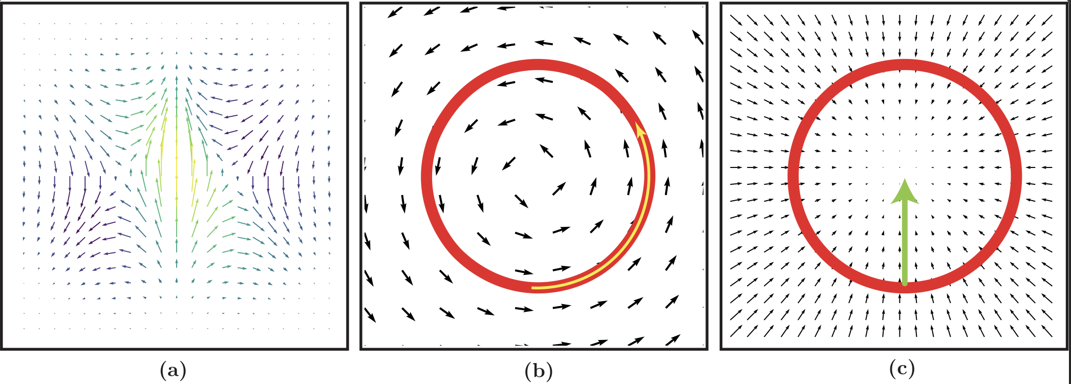
Figure 4: Access to the gradients (vector field) of the target distribution (a) is a natural information we can have for exploration. Most Markov transitions are diffusive in nature, i.e., the they can spend too much time near the initial point. In order to make large jumps away from the initial point, and into new, unexplored regions of the typical region, we need to exploit information about the geometry. Hamiltonian dynamics is the unique procedure for automatically generating this coherent exploration for sufficiently well-behaved target distributions. It not only allows efficient movement in the neighborhood of a mode (b) but also towards the mode that needs to be explored (c). The figure is inspired from Betancourt [2018].

2.1.3 Hamiltonian Dynamics

In Hamiltonian dynamics, we describe a system using a function called the Hamiltonian, which usually represents the total energy (kinetic + potential) of the system. Hamiltonian dynamics uses coordinates (where something is) and momentum (how fast it’s moving and in what direction) to describe motion. This shift helps in analyzing complex systems more easily [Betancourt, 2018].

Consider, for example, a typical problem of exploring the target distribution density during optimization. Usually, the information we have is the differential structure of the target distribution which we can query through the gradient of the target distribution density. In particular, the gradient defines a vector field in parameter space sensitive to the structure of the target distribution Fig.˜4(a). The gradients, however, can only guide us towards the parametrization-sensitive neighborhood like towards the mode (high density region)Fig.˜4(c), but not in the parameterization-invariant neighborhoods. To ensure, we can explore all regions of the distribution we need to ensure a coherent exploration of the geometry of the typical set (the red rings in Fig.˜4b,c).

Following Betancourt [2018], we can think of this exploration as if launching a satellite in a stable orbit around a planet. To ensure the satellite stays within the orbit, we need to give sufficient momentum to counteract the gravitational attraction. In probabilistic perspective, this gravitational pull can be thought of as the gradient vector field guiding the exploration. If sufficient momentum is not injected, the exploration will always be moving towards the mode. We can introduce momentum in the probabilistic structure using auxillary momentum parameters. But we have to ensure that the probabilistic structure ensures conservative dynamics. Conservative dynamics in physical systems requires that volumes are exactly preserved. Hamiltonian dynamics provides us this procedure to introduce such auxillary momentum.

Phase space.

Instead of dealing with target parameter space, the state of a Hamiltonian system is represented in a space called phase space, where each point corresponds to a unique combination of position and momentum. The points are lifted from the parameter space to the phase space, undergoes trajectory exploration and then projected back to the parameter space.

Hamilton’s equation.

The dynamics of the system are governed by two main equations, known as Hamilton’s equations, which tell us how the position and momentum change over time. They can be written as:

$$\frac{dq}{dt}=\frac{\partial H(q,m)}{\partial q}\;,\;\frac{dm}{dt}=-\frac{\partial H(q,m)}{\partial m}$$ (6)

where $q$ is the generalized coordinate (position), $m$ is the generalized momentum and $H(q,m)$ is the Hamiltonian, representing the total energy of the system.

Hamiltonian function.

The Hamiltonian function $H(q,m)$ represents the total energy of the system and is typically given by:

$$H(q,m)=U(q)+K(m)$$ (7)

where $U$ is the potential energy, often related to the negative log-likelihood of the target distribution and $K$ is the kinetic energy. When combined with stochastic elements, it leads to methods like Hamiltonian Monte Carlo, which are used for sampling from complex distributions. We will explore Hamiltonian Monte Carlo in the coming sections.

2.2 Monte Carlo integration

Estimating high-dimensional integrals e.g., $I=\int_{\Omega}f(x)dx$ is usually achieved by numerical integration methods like Monte Carlo. Monte Carlo estimator of an integral $I$ has a form:

$$I_{N}=\frac{1}{N}\sum_{i=o}^{N-1}\frac{f(\mathbf{x}_{i})}{p(\mathbf{x}_{i})}$$ (8)

where $f(\cdot)$ is the function to be integrated over the domain $\Omega$, $p$ represents the proposal distribution to extract $N$ samples $\mathbf{x}_{i}$ where $i\in{0,\ldots,N-1}$. Such estimation is error prone and is visible as noise in rendered images using physically based light transport rendering. Several variance reduction strategies are proposed in the literature Veach [1998]. Importance sampling is one such strategy and is known to reduce the variance. To perform importance sampling, samples are drawn from a proposal distribution and weighted to be used in the estimator Eq.˜8. This strategy can be quite efficient if proposal distribution is well-matched with the target distribution. However, finding a right proposal distribution is not always trivial. Also, importance sampling can become impractical for high-dimensional problems where finding a good proposal distribution is challenging. This is where MCMC sampling methods plays a crucial role.

2.3 MCMC sampling methods

MCMC method is a powerful tool to generating samples from complex arbitrary distributions. These samples can then be used to approximate integrals such as Eq.˜8. MCMC is a class of algorithms that generate samples from a target distribution by constructing a Markov chain that has the target distribution as its equilibrium distribution. MCMC algorithm works as follows:

• Initialization: Start with an initial state $\mathbf{x}_{0}$

• Transition: Define a transition mechanism (often a probability distribution) to move from the current state $\mathbf{x}_{t}$ to a new state $\mathbf{x}_{t+1}$. Common algorithms include the Metropolis-Hastings algorithm [Veach and Guibas, 1997].

• Stationarity: Ensure that the Markov chain has the target distribution as its stationary distribution. Over time, the distribution of the samples from the chain will converge to the target distribution.

• Sampling: Collect samples after a burn-in period (initial samples are discarded to allow the chain to converge).

In this part, we will introduce Metropolis-Hastings, Langevin Monte Carlo and Hamilotnian Monte Carlo sampling methods. MCMC sampling methods can be used for very complex and high-dimensional distributions where direct sampling is difficult. Different MCMC algorithms can be tailored for specific types of target distributions. We will also highlight their shortcomings e.g., MCMC methods require many iterations to converge to the target distribution, which can be computationally expensive.

2.3.1 Metropolis-Hastings algorithm

The Metropolis-Hastings algorithm is an MCMC method for obtaining a sequence of samples from a probability distribution from which direct sampling is difficult. Here’s a step-by-step algorithm for the Metropolis-Hastings method:

• Initialize the state,

• For each iteration, propose a new state from the proposal distribution,

• Compute the acceptance ratio and accept or reject the proposed state based on a random draw from a uniform distribution.

A python pseudo code is shown here:

Listing 1: Python example

⬇

import numpy as np

import matplotlib.pyplot as plt

# Target distribution: e.g. 2D Gaussian

def target_distribution(x):

return np.exp(-0.5 * np.dot(x, x))

# Proposal distribution: e.g. Gaussian with mean at the current state

def proposal_distribution(x, sigma=1.0):

return x + np.random.normal(scale=sigma, size=x.shape)

# Metropolis-Hastings algorithm

def metropolis_hastings(initial_state, num_samples, proposal_sigma):

samples = []

x_t = np.array(initial_state)

for _ in range(num_samples):

x_star = proposal_distribution(x_t, proposal_sigma)

acceptance_ratio = min(1, target_distribution(x_star) / target_distribution(x_t))

if np.random.rand() < acceptance_ratio:

x_t = x_star

samples.append(x_t.copy())

return np.array(samples)

# Parameters

initial_state = [0.0, 0.0]

num_samples = 10000

proposal_sigma = 1.0

# Generate samples using Metropolis-Hastings

samples = metropolis_hastings(initial_state, num_samples, proposal_sigma)

print(samples.shape)

# Plot the samples

plt.figure(figsize=(8, 8))

plt.plot(samples[:, 0], samples[:, 1], ’o’, markersize=1)

plt.title(’Metropolis-Hastings Samples’)

plt.xlabel(’x[0]’)

plt.ylabel(’x[1]’)

plt.show()

2.3.2 Langevin Monte Carlo sampling

Langevin Monte Carlo (LMC) is a class of Markov Chain Monte Carlo (MCMC) algorithms that generate samples from a probability distribution of interest by simulating the Langevin Equation. It leverages the gradient of the log-probability (log-likelihood) to guide the sampling process more effectively. The update rule for LMC is given by:

$$\mathbf{x}_{t+1}=\mathbf{x}_{t}+\frac{\tau^{2}}{2}\nabla\log p(\mathbf{x}_{t})+\tau\xi_{t}$$ (9)

where $\mathbf{x}_{t}$ is a current sample, $\tau$ is the time step, $\nabla\log p(\mathbf{x}_{t})$ is the log-probability of the target distribution $p$ and $\xi_{t}$ is the noise term, typically drawn from a standard normal distribution $\mathcal{N}(0,I)$.

2.3.3 Annealed Langevin Monte Carlo sampling

Annealed Langevin Monte Carlo (ALMC) is a variant of LMC that introduces an annealing schedule. Annealing is a process where the "temperature" of the system is gradually decreased, starting from a high value (which allows the sampler to explore the state space more freely) and gradually lowering it to focus more on high-probability regions.

In ALMC, the target distribution is tempered by introducing a temperature parameter T, and this parameter is gradually annealed. The tempered distribution is given by: $p_{T}(\mathbf{x})\propto p(\mathbf{x})^{1/T}$. The update rule for ALMC is similar to LMC but incorporates the temperature parameter:

$$\mathbf{x}_{t+1}=\mathbf{x}_{t}+\frac{\tau^{2}}{2T}\nabla\log p(\mathbf{x}_{t})+\tau\xi_{t}$$ (10)

where $T$ decreases over time according to a schedule. Typically, $T$ starts from a high value and gradually decreases to 1.

While LMC is effective for sampling from unimodal distributions or when the modes are well-separated and the gradient information is reliable. On the other hand, ALMC is useful for sampling from multimodal distributions where the modes are not easily separable, as the annealing process helps in exploring the global structure before focusing on high-probability regions.

2.3.4 Hamiltonian Monte Carlo sampling

A direct connection between SDEs and MCMC is also found in the Hamiltonian Monte Carlo (HMC) method. HMC leverages concepts from physics, particularly Hamiltonian dynamics, which are described by differential equations. The dynamics are typically simulated using numerical methods that solve differential equations, ensuring efficient exploration of the target distribution.

HMC offers a powerful set of Markov transitions that are capable of performing well over a large class of target distributions. The major challenge in implementing HMC is generating the Hamiltonian trajectories themselves. Formally, integrating along the vector field define by Hamiltonian equations is equivalent to solving ordinary differential equations in phase space. However, most of the ODE solvers can drift away from the trajectories accumulating error over time.

We can, however, use the geometry of the phase space to construct extremely powerful family of numerical solvers known as the use symplectic integrators [Leimkuhler and Reich, 2005, Hairer et al., 2013]. These integrators are robust to drift and enable high-performance implementaiton of HMC method. Symplectice integrators are straightforward to implement in practice. If the probabilistic distribution of the momentum is independent of the position, then we can employ a simple leapfrog integrator. Given a time discretization, the leapfrog integrator simulates the exact trajectory by precise interleaving of discrete momentum and position updates that ensures exact volume preservation on phase space.

2.3.5 Discussion

In summary, MH is simple and flexible but can be inefficient for complex or high-dimensional problems. Langevin dynamics improves on MH by using gradient information, but requires smoothness and introduces discretization issues. HMC is the most efficient in high dimensions, particularly for smooth distributions, but is computationally expensive and requires careful tuning. We provide a detailed comparison among these methods along different aspects in Table˜1.

MH can be applied to a wide variety of distributions as long as you can evaluate the target distribution’s density up to a normalizing constant. The algorithm is conceptually straightforward and easy to implement. It can be used with any proposal distribution, allowing for customization to the problem at hand. It guarantees to converge to the true target distribution (if ergodic conditions are met). However, if the proposal distribution is poorly chosen, it may explore the space inefficiently (slow mixing and high autocorrelation). The performance of the algorithm depends heavily on the proposal distribution and its scale. Poor choices can result in high rejection rates. MH can be slow for high-dimensional problems, as proposals often move inefficiently in large spaces.

Langevin dynamics can take advantage of the gradient of the log-posterior, making it more efficient than random-walk methods like MH, especially for smooth target distributions. The gradient information helps proposals move toward high-probability regions, leading to faster exploration of the space. Proposals are more informed, so they generally require less tuning than vanilla MH. On the other hand, calculating the gradient can be expensive, especially in high-dimensional or complex models. LMC assumes that the log-posterior is differentiable and smooth. It may not work well with highly non-smooth distributions. Since Langevin dynamics is a continuous process, discretizing it to use in practice introduces bias unless corrected (e.g., through the Metropolis-adjusted Langevin algorithm, MALA).

Finally, HMC can make large, informed jumps in the parameter space, allowing it to explore high-dimensional spaces much more efficiently than random-walk-based methods like MH. The proposals are designed to make larger, more informed steps, which reduces autocorrelation and improves convergence speed. Like Langevin dynamics, HMC leverages gradients to propose new states, making it well-suited for smooth, differentiable posterior distributions. However, HMC depends on parameters like step size and the number of leapfrog steps. Poor tuning can lead to either rejection of proposals or inefficient exploration. Each iteration requires solving Hamiltonian dynamics via the leapfrog integrator, which is computationally expensive in high-dimensional models. HMC can struggle to explore multimodal distributions, as its trajectories are deterministic and may not easily traverse between modes.

Aspect	Metropolis-Hastings (MH)	Langevin Monte Carlo (LMC)	Hamiltonian Monte Carlo (HMC)
Efficiency	Low for high dimensions (random walk behavior)	Better than MH, guided by gradients	Very efficient, especially in high dimensions
Gradient usage	No	Yes	Yes
Autocorrelation	High, especially with poor proposals	Lower than MH	Very low due to long, informed trajectories
Tuning required	Yes (proposal distribution)	Yes (step size for discretization)	Yes (step size, number of leapfrog steps)
Scalability	Poor in high dimensions	Moderate	Good for large dimensions
Applicability	Very general	Requires smoothness and gradients	Requires smoothness and gradients
Computational cost per step	Low	Moderate	High
Convergence	Slower, especially for bad proposals	Faster, thanks to gradient guidance	Fast, but sensitive to parameter settings
Suitability for multimodality	Decent, but still slow	May struggle with multimodal targets	Poor, deterministic paths struggle with multiple modes

Table 1: Comparing MH, LMC and HMC sampling methods

3 MCMC in rendering

Physically based rendering algorithms simulate the behavior of light to turn scene representations describing object shape and optical properties into realistic images. For this, they must simulate various physical laws that can be roughly classified into transport and scattering, i.e., the propagation of light through space, and its local interaction with the objects comprising the scene. From a mathematical perspective, the entire problem reduces to evaluating a series of high-dimensional integrals to determine the radiance $I_{j}$ received by each pixel $j$ of a virtual camera observing the scene, i.e.:

$$I_{j}=\int_{\Omega}f_{j}(\mathbf{x})\,\mathrm{d}\mathbf{x}.$$ (11)

The function $f_{j}$ characterizes this process for given pixel $j$, while $\Omega$ depends on the specific formulation and algorithm being used. The dimension of $\Omega$ is generally proportional to the number of subsequent scattering events that should be considered. This number can be rather large and ranges from tens to many thousands of dimensions to deal with highly scattering materials like clouds, milk, skin, etc. For this reason, Monte Carlo methods have become the method of choice in the last decades.

3.1 Path-space

Veach [1998] introduced a particularly general variant of the integration problem from Equation 11 known as the path space formulation that we discuss here for the special case of scenes containing only surfaces (i.e., lacking volumetric effects). It decomposes the integration domain $\Omega$ into union of subspaces:

$$\Omega\coloneqq\bigcup_{n=2}^{\infty}\Omega_{n},\text{ and}$$

$$\Omega_{n}\coloneqq\left\{\mathbf{x}_{1}\cdots\mathbf{x}_{n}\;\middle|\;\mathbf{x}_{1},\ldots,\mathbf{x}_{n}\in\mathcal{M}\right\},$$ (12)

where $\mathcal{M}$ is the set of surfaces within the virtual scene. Elements $\bar{\mathbf{x}}=\mathbf{x}_{1},\ldots\mathbf{x}_{n}\in\Omega_{n}$ referred to as paths denote potential trajectories that light can take while traveling from the light source towards the virtual sensor.

The pixel intensity $I_{j}$ is given by

$$I_{j} =\int_{\Omega_{2}}f(\mathbf{x}_{1}\mathbf{x}_{2})\,\mathrm{d}A(\mathbf{x}_{1},\mathbf{x}_{2})\ +\int_{\Omega_{3}}f(\mathbf{x}_{1}\mathbf{x}_{2}\mathbf{x}_{3})\,\mathrm{d}A(\mathbf{x}_{1},\mathbf{x}_{2},\mathbf{x}_{3})+\ldots.$$ (13)

Because some paths carry more illumination from the light source to the camera than others, the integrand $$f:\Omega\to\mathbb{R} I_{j} f$$ is needed to quantify their “light-carrying capacity”; its definition varies based on the number of input arguments and is given by Equation (15). The total illumination arriving at the camera is often written more compactly as an integral of over the entire path space, i.e.:

$$\eqqcolon\int_{\Omega}f(\bar{\mathbf{x}})\,\mathrm{d}A(\bar{\mathbf{x}}).$$ (14)

The definition of the weighting function $f$ consists of a product of terms—one for each vertex and edge of the path:

$$f(\mathbf{x}_{1}\cdots\mathbf{x}_{n})=L_{e}(\mathbf{x}_{1}\to\mathbf{x}_{2})\left[\prod_{k=2}^{n-1}G(\mathbf{x}_{k-1}\leftrightarrow\mathbf{x}_{k})\,f(\mathbf{x}_{k-1}\to\mathbf{x}_{k}\to\mathbf{x}_{k+1})\right]G(\mathbf{x}_{n-1}\leftrightarrow\mathbf{x}_{n})\,W_{e}^{(j)}(\mathbf{x}_{n-1}\to\mathbf{x}_{n}).$$ (15)

The arrows in the above expression symbolize the symmetry of the geometric terms as well as the flow of light at vertices. $\mathbf{x}_{i}\to\mathbf{x}_{i+1}$ can also be read as a spatial argument $\mathbf{x}_{i}$ followed by a directional argument $\overrightarrow{\mathbf{x}_{i}\mathbf{x}_{i+1}}$. Figure 5 shows an example light path and the different weighting terms. We summarize their meaning below:

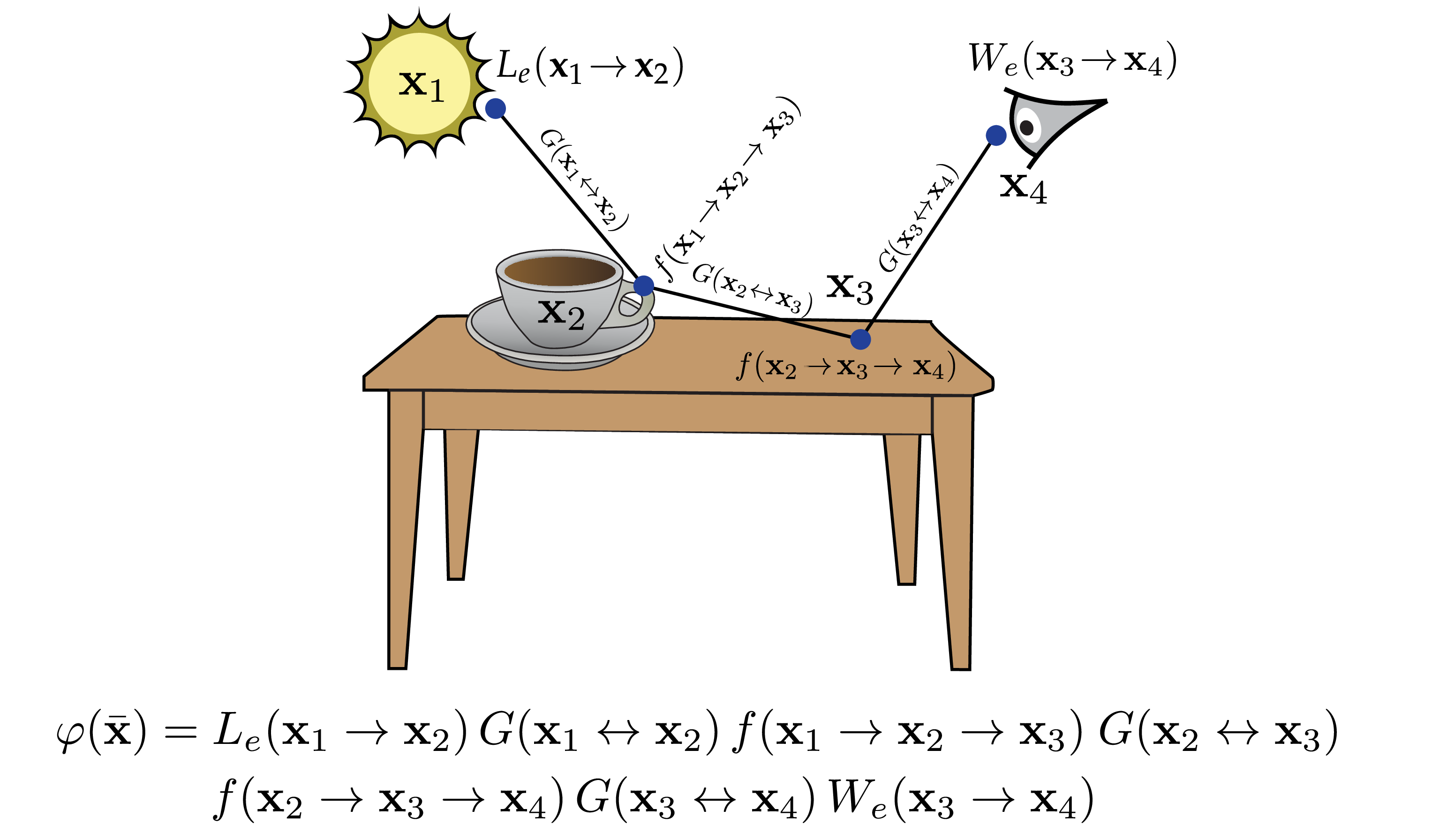
Figure 5: Illustration of a simple light path with four vertices and its corresponding weighting function.

• The first term $L_{e}(\mathbf{x}_{1}\to\mathbf{x}_{2})$ is the emission profile of the light source. This term models the amount of light emitted from position $\mathbf{x}_{1}$ traveling towards $\mathbf{x}_{2}$. It equals zero when $\mathbf{x}_{1}$ is not located on a light source.

• The last term $W_{e}^{j}(\mathbf{x}_{n-1}\to\mathbf{x}_{n})$ is the sensitivity profile of pixel $j$ of the camera; we can think of the pixel grid as an array of sensors, each with its own profile function.

• $G(\mathbf{x}\leftrightarrow\mathbf{y})$ is the geometric term, which specifies the differential amount of illumination carried along segments of the light path. Among other things, it accounts for visibility: when there is no unobstructed line of sight between $\mathbf{x}$ and $\mathbf{y}$, $G$ evaluates to zero.

• $f(\mathbf{x}_{k-1}\to\mathbf{x}_{k}\to\mathbf{x}_{k+1})$ is the bidirectional scattering distribution function (BSDF), which specifies how much of the light that travels from $\mathbf{x}_{k-1}$ to $\mathbf{x}_{k}$ then scatters towards position $\mathbf{x}_{k+1}$. This function characterizes the material appearance of an object (e.g., whether it is made of wood, plastic, concrete, etc.).

Over the last 40 years, considerable research has investigated realistic expressions for the terms listed above. In this article, we do not discuss their internals and prefer to think of them as black box functions that can be queried by the rendering algorithm. This is similar to how rendering software is implemented in practice: a scene description might reference a particular material (e.g., car paint) whose corresponding function $f$ is provided by a library of material implementations. The algorithm accesses it through a high-level interface shared by all materials, but without specific knowledge about its internal characteristics.

3.2 Multiple Importance Sampling

Many Monte Carlo rendering methods can be interpreted as sampling strategies that generate paths $\bar{\mathbf{x}}$ according to a carefully chosen probability distribution $p$. Ideally, such a strategy would employ a density function $p$ that is approximately proportional to the integrand $f$, thereby producing renderings with low variance. However, such strategies are unfortunately not available in general.

A general building block of sampling strategies are random walks: for example, starting with the endpoint vertex $\mathbf{x}_{n-1}$ (the position of the camera), we could randomly sample the predecessor $\mathbf{x}_{n-2}$ followed by $\mathbf{x}_{n-3}$, etc. Similarly, we could generate a random sample on the light source $\mathbf{x}_{1}$ and then work our way towards the camera. Paths could also be sampled from both sides or the middle (e.g. a window of a room). Combinations of such walks produce a family of sampling strategies with useful properties.

Given a set of sampling strategies on a consistent domain $\Omega$, it is possible to evaluate and compare their densities to combine them effectively. This is the key insight of a widely used technique known as multiple importance sampling (MIS) [Veach and Guibas, 1995].

Suppose two statistical estimators of the pixel intensity $I_{j}$ are available. These estimators can be used to generate two light paths $\bar{\mathbf{x}}_{1}$ and $\bar{\mathbf{x}}_{2}$, which have path space probability densities $p_{1}(\bar{\mathbf{x}}_{1})$ and $p_{2}(\bar{\mathbf{x}}_{2})$, respectively. The corresponding MC estimates are given by

$$\langle I_{j}^{(1)}\rangle=\frac{f(\bar{\mathbf{x}}_{1})}{p_{1}(\bar{\mathbf{x}}_{1})}\quad\text{and}\quad\langle I_{j}^{(2)}\rangle=\frac{f(\bar{\mathbf{x}}_{2})}{p_{2}(\bar{\mathbf{x}}_{2})}.$$

To obtain a combined estimator, we could simply average these estimators, i.e.:

$$\langle I_{j}^{(3)}\rangle\coloneqq\frac{1}{2}\big(\langle I_{j}^{(1)}\rangle+\langle I_{j}^{(2)}\rangle\big).$$

However, this is not a good idea, since the combination is affected by the variance of the worst ingredient estimator. Instead, MIS combines estimators using weights that are related to the underlying sample density functions:

$$\langle I_{j}^{(4)}\rangle\coloneqq w_{1}(\bar{\mathbf{x}}_{1})\langle I_{j}^{(1)}\rangle+w_{2}(\bar{\mathbf{x}}_{2})\langle I_{j}^{(2)}\rangle.$$

A particularly simple weighting function known as the balance heuristic has the following expression for two input strategies:

$$w_{i}(\bar{\mathbf{x}})\coloneqq\frac{p_{i}(\bar{\mathbf{x}})}{p_{1}(\bar{\mathbf{x}})+p_{2}(\bar{\mathbf{x}})}.$$ (16)

Veach originally showed that no other choice of positive weighting functions can significantly improve upon the balance heuristic. Ivo et al. [2019] later introduced a generalization to negative weights that provably minimizes variance in the general case.

Combinations of multiple sampling techniques are often an effective way to reduce variance to an acceptable amount. Yet, even such combinations can fail in simple cases, as we will discuss next.

3.3 Limitations of Monte Carlo Path Sampling

Ultimately, all Monte Carlo path sampling techniques can be seen to compute integrals of the weighting function $f$ using a variety of importance sampling techniques that evaluate $f$ at many randomly chosen points throughout the domain $\Omega$.

Certain input, particularly scenes containing metal, glass, or other shiny surfaces, can lead to integrals that are difficult to evaluate. Depending on the roughness of the surfaces, the integrand can take on large values over small regions of the integration domain. Surfaces of lower roughness lead to smaller and higher-valued regions, which eventually collapse to lower-dimensional sets with singular integrands as the surface roughness tends to zero. This case where certain paths cannot be sampled at all is known as the problem of insufficient techniques  Kollig and Keller [2002].

Figure 6: Illustration of the difficulties of sequential path sampling methods when rendering caustic patterns at the bottom of a swimming pool. (a, b): Unidirectional techniques sample light paths by executing a random walk consisting of alternating transport and scattering steps. The only way to successfully complete a path in this manner is to randomly “hit” the light source or camera, which happens with exceedingly low probability. (c): Bidirectional techniques trace paths from both sides, but in this case they cannot create a common vertex at the bottom of the pool to join the partial light paths.

Convergence problems arise whenever high-valued regions receive too few samples. Depending on the method used, this manifests as objectionable noise or other visual artifacts in the output image that gradually disappear as the sample count $N$ tends to infinity. However, due to the slow convergence rate of MC integration (typical error is $\mathcal{O}(N^{-0.5})$), it may not be an option to wait for the error to average out. Such situations can force users of rendering software to make unrealistic scene modifications (e.g., disabling certain light interactions), compromising realism in exchange for obtaining converged-looking results within a reasonable time.

Figure 6 illustrates the behavior of several path sampling methods when rendering caustics at the bottom of the swimming pool. This refers to the light patterns resulting from focused refraction by ripples in the water surface.

In Figure 6 (a), light tracing samples paths starting from the light source. This eventually leads to a path segment that leaves the pool, but it never hits the camera aperture and thus cannot contribute to the output image. Path tracing in Figure 6 (b) generates paths from the opposite end and also remains extremely inefficient. Assuming for simplicity that rays leave the pool with a uniform distribution in the probability of hitting the sun with an angular diameter of $\sim 0.5^{\circ}$ is on the order of $10^{-5}$. Bidirectional sampling methods (Figure 6 (c)) tracing from both sides also fail: they generate two vertices at the bottom of the pool as shown in the figure, but these cannot be connected: the resulting edge would be fully contained in a surface rather than representing transport between surfaces.

The main difficulty in scenes like this is that caustic paths are tightly constrained: they must start on the light source, end on the aperture, and satisfy Snell’s law in two places. Sequential sampling approaches are able to satisfy all but one constraint and run into issues when there is no way to complete the majority of paths.

Paths like the one examined in Figure 6 lead to poor convergence in other settings as well; they are collectively referred to as specular–diffuse–specular (SDS) paths due to the occurrence of this sequence of interactions in their path classification. SDS paths occur in common situations such as a tabletop seen through a drinking glass standing on it, a bottle containing shampoo or other translucent liquid, a shop window viewed and illuminated from outside, as well as scattering inside the eye of a virtual character. Even in scenes where these paths do not cause dramatic effects, their presence can lead to excessively slow convergence in rendering algorithms that attempt to account for all transport paths. It is important to note that while the SDS class of paths is a well-studied example case, other classes (e.g., involving glossy interactions) can lead to many similar issues. It is desirable that rendering methods are robust to such situations.

Correlated path sampling techniques based on MCMC offer an attractive way to approach such challenges because they provide a framework in which the costly discovery of an SDS path can be amortized by exploring its neighborhood.

3.4 Metropolis Light Transport

In 1997, Veach and Guibas proposed an unusual rendering technique named Metropolis Light Transport [Veach and Guibas, 1997], which applies the Metropolis-Hastings algorithm to Equation 14. Using correlated samples and highly specialized mutation rules, their approach enables more systematic exploration of the integration domain, avoiding many of the problems encountered by methods based on standard Monte Carlo and sequential path sampling.

MCMC rendering methods in general sample light paths proportional to the amount they contribute to the pixels of the final rendering; by increasing the pixel brightness in this way during each iteration, these methods effectively compute a 2D histogram of the marginal distribution of $f$ over pixel coordinates. This is exactly the image to be rendered up to a global scale factor, which can be recovered using a traditional MC sampling technique. The main difference among these algorithms is the underlying state space, as well as the employed set of mutation rules.

Figure 7: MLT operates on top of path space, which permits the use of a variety of mutation rules that are motivated by important physical scattering effects. The top row illustrates ones that are useful when rendering a scene involving a glass object on top of a diffuse table. The bottom row is the swimming pool example from Figure 6. In each example, the original path is black, and the proposal is highlighted in blue.

MLT distinguishes between mutations that change the structure of the path and perturbations that move the vertices by small distances while preserving the path structure, both using the building blocks of bidirectional path tracing to sample paths. One of the following operations is randomly selected in each iteration:

1. Bidirectional mutation: This mutation replaces a segment of an existing path with a new segment (possibly of different length) generated by a random walk strategy. This rule generally has a low acceptance ratio but it is essential to guarantee ergodicity of the resulting Markov Chain.

2. Lens subpath mutation: The lens subpath mutation is similar to the previous mutation but only replaces the lens subpath, which is defined as the trailing portion of the light path matching the regular expression [^S]S*E.

3. Lens perturbation: This transition rule shown in Figure 7a only perturbs the lens subpath rather than regenerating it from scratch. In the example, it slightly rotates the outgoing ray at the camera and propagates it until the first non-specular material is encountered. It then attempts to create a connection (dashed line) to the unchanged remainder of the path.

4. Caustic perturbation: The caustic perturbation (Figure 7b) works just like the lens perturbation, except that it proceeds in reverse starting at the light source. It is well-suited for rendering caustics that are directly observed by the camera.

5. Multi-chain perturbation: This transition rule (Figure 7c) is used when there are multiple separated specular interactions, e.g., in the swimming pool example encountered before. After an initial lens perturbation, a cascade of additional perturbations follows until a connection to the remainder of the path can finally be established.

The main downside of MLT is the severe effort needed to implement this method: several of the mutation and perturbation rules (including their associated proposal densities) are challenging to reproduce. Another problem is that a wide range of different light paths generally contribute to the output image. The MLT perturbations are designed to deal with specific types of light paths, but it can be difficult to foresee every kind in order to craft a suitable set of perturbation rules. In practice, the included set is insufficient.

3.5 Primary sample space MLT

While path space is a powerful foundation for reasoning about light transport, the resulting algorithms are notoriously difficult to implement. Kelemen et al. [2002] later showed that a much simpler approach can be used to directly combine MCMC sampling with existing MC rendering algorithms, making it possible to altogether avoid the complexities of path space. The main idea underlying their method named Primary Sample Space MLT (PSSMLT) is general and can also be applied to integration problems outside of rendering.

PSSMLT operates on top of an existing MC sampling technique that draws light paths $\bar{\mathbf{x}}$ from a target distribution. At the implementation level, such sampling techniques are usually implemented by warping uniformly distributed input samples $\mathbf{u}$ into the desired distribution. All randomness is provided by the input sample $\mathbf{u}$, while the warping steps are not only deterministic but usually even differentiable. In practice, the inverse transform method is almost always used to realize this warping step.

The rendering process can then be seen compute an integral of a function with with signature $\Psi:[0,1]^{n}\to\mathbb{R}$ that maps a vector of univariate samples to a pixel intensity estimate. By taking many estimates and averaging them to obtain a converged pixel intensity, path tracing is effectively integrating the estimator over a $n$-dimensional unit hypercube of “random numbers” denoted as primary sample space:

$$I_{j}=\int_{[0,1]^{n}}\Psi(\mathbf{\mathbf{u}})\,\mathrm{d}\mathbf{\mathbf{u}}.$$ (17)

The key idea of PSSMLT is to compute Equation (17) using MCMC integration on directly primary sample space, which leads to a trivial implementation, as all complications involving light paths and other rendering-specific details are encapsulated in the “black box” mapping $\Psi$ (Figure 8).

Figure 8: Primary Sample Space MLT performs mutations in an abstract random number space. A deterministic mapping $\Psi$ induces corresponding mutations in path space.

PSSMLT uses two types of mutation functions. The first is an independence sampler, i.e., it forgets the current state and switches to a new set of pseudorandom variates. This is needed to ensure that the Markov Chain is ergodic. The second is a local (e.g. Gaussian or similar) proposal centered around a current state $\mathbf{u}_{i}\in[0,1]^{n}$. Both are symmetric so that the proposal density cancels in the Metropolis-Hastings acceptance ratio.

PSSMLT uses independent proposals to find important light paths that cannot be reached using local proposals. When it finds one, local proposals are used to explore neighboring light paths which amortizes the cost of the search. This can significantly improve convergence in many challenging situations and is an important advantage of MCMC methods in general when compared to MC integration.

Another advantage of PSSMLT is that it explores light paths through a black box mapping $\Psi$ that already makes internal use of sophisticated importance sampling techniques for light paths, which in turn leads to an easier integration problem in primary sample space. The main disadvantage of this method is that its interaction with $\Psi$ is limited to a stream of pseudorandom numbers. It has no direct knowledge of the generated light paths, which prevents the design of more efficient mutation rules based on the underlying physics.

3.6 Hessian-Hamiltonian MLT

Light paths are often highly constrained because they must satisfy physical constraints at multiple vertices (Section 3.3). A consequence of such constraints is that the effective exploration of the neighborhood of a light path requires a concerted change to multiple coordinates at once. Simple isotropic transition densities that do not explicitly model dependencies between coordinates tend to be rejected following steps into low-valued regions of the integrand.

Later work on MCMC rendering algorithms introduced anisotropic proposals to alleviate these problems. Li et al. [2015] considered the behavior of Hamiltonian dynamics in a neighborhood of the integrand. When the integrand $f$ is locally approximated using a two-term Taylor expansion, a windowed HMC step reduces to a sample from a multivariate normal distribution, whose covariance can be computed from the Hessian matrix. The final method resembles MALA with an anisotropic proposal density.

4 MCMC in optimization

Stochastic gradient descent (SGD) methods are primarily used to optimize functions, particularly in training machine learning models where the objective is to minimize a loss function. SGD shares similarities with MCMC sampling methods in their iterative nature, especially in the context of Bayesian inference and machine learning [Chen et al., 2016]. In this part, we will lay down the similarites between both SGD and MCMC methods and review SGD algorithms driven by MCMC methods.

4.1 Bayesian inference

Bayesian inference is a method of statistical inference in which Bayes’ theorem is used to update the probability of a hypothesis as more evidence or data becomes available. It provides a principled way to combine prior knowledge (beliefs about parameters) with new data to make probabilistic conclusions about uncertain parameters or models. The foundations of Bayesian inference is Bayes’ theorem, which is expressed as:

$$p(\theta|\text{data})=\frac{p(\text{data}|\theta)p(\theta)}{p(\text{data})}$$ (18)

where

• $p(\theta|\text{data})$ is the posterior probability of the parameter $\theta$ given the observed data. This is what we want to infer. The posterior distribution combines the prior and likelihood to give an updated probability distribution of the parameter $\theta$ after observing the data.

• $p(\text{data}|\theta)$ is the likelihood, which represents how likely the observed data is under a given parameter $\theta$. The likelihood represents the probability of observing the data given a particular value of $\theta$. It is derived from the model and the observed data

• $p(\theta)$ is the prior probability, which reflects the prior belief about the parameter $\theta$ before seeing the data. It allows you to incorporate existing knowledge or assumptions about the parameter.

• $p(\text{data})$ is the evidence (or marginal likelihood), which normalizes the posterior and ensures that the probabilities sum to $1$. The evidence term is the probability of observing the data under all possible values of $\theta$. It is often treated as a normalizing constant and doesn’t affect the inference about $\theta$.

Bayesian inference provides a powerful framework for updating beliefs based on new data, handling uncertainty, and making probabilistic predictions. By leveraging both prior knowledge and data, it offers a flexible and rigorous approach to statistical inference.

4.2 Stochastic gradient descent (SGD)

SGD is an optimization algorithm that iteratively updates model parameters to minimize a loss function. It uses the gradient of the loss function with respect to the model parameters to guide the updates. In each iteration, a mini-batch of data is used to compute an approximate gradient, making the process stochastic. The update rule for SGD is:

$$\theta_{t+1}=\theta_{t}-\eta\nabla_{\theta}\mathcal{L}(\theta_{t})$$ (19)

where $\theta_{t}$ are the model parameters at iteration $t$, $\eta$ is the learning rate, $\nabla_{\theta}\mathcal{L}(\theta_{t})$ is the gradient of the loss function $\mathcal{L}$ with respect to $\theta_{t}$.

SGD is primarily used for deterministic optimization, It is efficient for large-scale machine learning problems due to its stochastic nature. However, it is prone to getting stuck in local minima or saddle points.

4.3 Stochastic Gradient Langevin Dynamics (SGLD)

SGLD is an algorithm that combines elements of SGD with Langevin dynamics [Welling and Teh, 2011], introducing a noise term to the parameter updates. This addition allows SGLD to perform both optimization and sampling from the posterior distribution in Bayesian inference. The update rule for SGLD is very similar to the SGD update rule from Eq.˜19 and is given by:

$$\theta_{t+1}=\theta_{t}-\frac{\eta}{2}\nabla_{\theta}\mathcal{L}(\theta_{t})+\sqrt{\eta}\xi_{t}$$ (20)

where $\theta_{t}$ are the model parameters at iteration $t$, $\eta$ is the learning rate, $\nabla_{\theta}\mathcal{L}(\theta_{t})$ is the gradient of the loss function $\mathcal{L}$ with respect to $\theta_{t}$ and $\xi_{t}$ is the noise term, typically drawn from a standard normal distribution $\mathcal{N}(0,I)$.

Listing 2: Python example

⬇

# Code snippet for SGLD update rule

import numpy as np

# Loss function and its gradient

def loss_function(theta):

return 0.5 * np.sum(theta**2)

def gradient_loss_function(theta):

return theta

# SGLD update rule

def sgld_update(theta, eta):

grad = gradient_loss_function(theta)

noise = np.random.normal(size=theta.shape)

theta = theta - 0.5 * eta * grad + np.sqrt(eta) * noise

return theta

# Parameters

theta = np.array([2.0, -3.0]) # Initial parameters

eta = 0.01 # Learning rate

num_iterations = 1000

# Perform SGLD

samples = []

for _ in range(num_iterations):

theta = sgld_update(theta, eta)

samples.append(theta.copy())

# Convert samples to numpy array for analysis

samples = np.array(samples)

# Plot the samples

import matplotlib.pyplot as plt

plt.plot(samples[:, 0], samples[:, 1], ’o-’, markersize=2)

plt.title(’SGLD Samples’)

plt.xlabel(’Theta[0]’)

plt.ylabel(’Theta[1]’)

plt.show()

SGD vs. SGLD.

There are some key differences:

• Objective: SGD aims to find a point estimate that minimizes the loss function, whereas, SGLD aims to sample from the posterior distribution of the model parameters, making it suitable for Bayesian inference.

• Update rule: SGD updates parameters using the gradient of the loss function with respect to the parameters. SGLD, on the other hand, Updates parameters using the gradient of the loss function and adds a noise term to ensure stochasticity.

• Noise term: SGD does not include an explicit noise term in the update rule. SGLD includes a noise term, which helps in exploring the parameter space more thoroughly and escaping local minima.

• Applications: SGD is used for deterministic optimization tasks, such as training neural networks, whereas, SGLD is used for probabilistic modeling and Bayesian inference, where sampling from the posterior distribution is required.

4.4 Bayesian inference using SGD

Performing Bayesian inference using Stochastic Gradient Descent (SGD) combines the ideas from Bayesian statistics with optimization techniques like SGD. The general idea is to approximate the posterior distribution over model parameters using gradient-based methods. This approach is particularly useful when exact Bayesian inference (like through Markov Chain Monte Carlo) is computationally infeasible for large datasets or complex models.

Maximum A Posteriori (MAP) Estimation using SGD

MAP estimation is a point estimate method in Bayesian inference. Instead of finding the full posterior distribution, we find the parameter value that maximizes the posterior distribution. The MAP objective is:

$$\theta_{MAP}=\arg\max_{\theta}p(\theta|\text{data})=\arg\max_{\theta}p(\text{data}|\theta)p(\theta)$$ (21)

Taking the logarithm of the posterior (since log is a monotonic function), this becomes:

$$\theta_{MAP}=\arg\max_{\theta}(\log p(\text{data}|\theta)+\log p(\theta))$$ (22)

Here, SGD can be used to optimize the MAP objective by computing gradients with respect to $\theta$, where $\log p(\text{data})$ is the likelihood (often minimized using SGD), and $p(\theta)$ is the prior (often treated as a regularization term, like $\mathcal{L}_{2}$ regularization).

To implement this optimization, we start with an initial guess for $\theta$. Then we use SGD Eq.˜19 to update the parameters by following the gradient of the posterior:

$$\theta_{t+1}=\theta_{t}-\eta\nabla_{\theta}(-\log p(\text{data}|\theta)-\log p(\theta))$$ (23)

where $\eta$ is the learning rate.

Using SGLD.

SGLD adds noise to the gradient updates from SGD to simulate Langevin dynamics, which helps approximate the posterior distribution instead of just finding a point estimate. The update rule for SGLD from Eq.˜20 is:

$$\theta_{t+1}=\theta_{t}-\eta\nabla_{\theta}(-\log p(\text{data}|\theta)-\log p(\theta))+\sqrt{\eta}\xi_{t}$$ (24)

where $\xi_{t}$ is a Gaussian noise with zero mean and unit variance. The injected noise ensures that the parameter updates sample from the posterior distribution rather than simply converging to a single point (as in MAP estimation). Over time, this stochastic process approximates the posterior distribution. In the next section, we look at Bayesian (variational) inference using neural networks. In this method, you approximate the posterior distribution with a simpler distribution (often Gaussian) and minimize the divergence between the true posterior and the approximate one.

5 MCMC in generative modeling

Diffusion models [Sohl-Dickstein et al., 2015] are the very backbone of modern generative AI pipelines and they are built on the very foundations of MCMC methods. In this part, we start by showing how MCMC can be seen as a primitive generative model. We briefly introduce evidence lower bound (ELBO), variational autoencoders (VAEs) and Hierarchical variational autoencoders (HVAEs) that lays the foundations for the variational diffusion models. We then introduce energy-based models which are known to be very flexible We then introduce score-based diffusion models that are driven by the SDEs [Song et al., 2021]. During this part, we will walk through the skeleton code that will result in a fully functional diffusion model for visual content creation.

Table 2: Commonly used notations throughout the document.

Notation	Description
$\mathbf{x},\mathbf{z}$	input (observed) data, latent space variables
$p(\mathbf{x})$	distribution of the observed data or likelihood of all observed $\mathbf{x}$ or the target distribution
$\log p(\mathbf{x})$	evidence or log-likelihood of the data
$q(\mathbf{z}|\mathbf{x})$	ground truth posterior (encoder) that defines the distribution of latent variables $\mathbf{z}$ over observed samples $\mathbf{x}$
$q_{\phi}(\mathbf{z}|\mathbf{x})$	variational posterior (encoder) distribution with parameters $\phi$ that we seek to optimize to match the ground truth $q(\mathbf{z}|\mathbf{x})$
$p_{\theta}(\mathbf{x}|\mathbf{z})$	decoder distribution parameterized by learnable parameters $\theta$

5.1 From variatonal autoencoders to variational diffusion models

The keyword variational is used in mathematical analysis when we deal with maximizing or minizming functionals. Our focus is likelihood-based generative models where the idea is to learn a model that maximizes the likelihood $p(\mathbf{x})$ of all observed data $\mathbf{x}$. We can imagine a joint distribution $p(\mathbf{x},\mathbf{z})$ that models the joint probability of the observed samples and their latent variables. There are two ways we can manipulate this joint distribution to recover the likelihood of the observed data distribution $p(\mathbf{x})$; we can explicitly marginalize the latent variable $\mathbf{z}$:

$$p(\mathbf{x})=\int p(\mathbf{x},\mathbf{z})d\mathbf{z}$$ (25)

which requires integrating over all latent variables $\mathbf{z}$ or, we can use the chain rule of the probability;

$$p(\mathbf{x})=\frac{p(\mathbf{x},\mathbf{z})}{p(\mathbf{z}|\mathbf{x})}$$ (26)

which requires access to the ground truth encoder $q(\mathbf{z}|\mathbf{x})$. Both methods of maximizing the likelihood are intractable when using complex models.

5.1.1 Evidence lower bound (ELBO).

Instead of focusing on directly maximizing the likelihood $p(\mathbf{x})$, we can work with the evidence; the log-likelihood $\log p(\mathbf{x})$. The ELBO represents the lower bound on the evidence. Let us build this lower bound in few steps. By definition ELBO is given by:

$$\mathbb{E}_{q_{\phi}(\mathbf{z}|\mathbf{x})}\left[\log\frac{p(\mathbf{x},\mathbf{z})}{q_{\phi}(\mathbf{z}|\mathbf{x})}\right]$$ (27)

Looking at Eqs.˜26 and 27, we can derive the evidence in the form (see Luo [2022] for details):

$$\underbrace{\log p(\mathbf{x})}_{\text{Evidence}}=\underbrace{\mathbb{E}_{q_{\phi}(\mathbf{z}|\mathbf{x})}\left[\log\frac{p(\mathbf{x},\mathbf{z})}{q_{\phi}(\mathbf{z}|\mathbf{x})}\right]}_{\text{ELBO}}+\underbrace{D_{KL}(q_{\phi}(\mathbf{z}|\mathbf{x})||q(\mathbf{z}|\mathbf{x}))}_{\text{Distance}}$$ (28)

where $D_{KL}(q_{\phi}(\mathbf{z}|\mathbf{x})||q(\mathbf{z}|\mathbf{x}))$ is a distance metric. This distance metric is the KL-divergence between the ground truth $q(\mathbf{z}|\mathbf{x})$ and our flexible approximate variational distribution $q_{\phi}$ with parameters $\phi$ that we seek to optimize. In other words, $q_{\phi}$ seeks to approximate the true posterior $q(\mathbf{z}|\mathbf{x})$.

Since the second summand on the RHS of Eq.˜28 is a distance metric, it is always positive. Therefore, the evidence is always higher than the ELBO term. In short, the evidence has a direct relationship wrt the ELBO term:

$$\log p(\mathbf{x})\geq\mathbb{E}_{q_{\phi}(\mathbf{z}|\mathbf{x})}\left[\log\frac{p(\mathbf{x},\mathbf{z})}{q_{\phi}(\mathbf{z}|\mathbf{x})}\right]$$ (29)

which implies that the ELBO is the lower bound of the evidence.

Note that the likelihood $p(\mathbf{x})$ of our data—and therefore our evidence term $\log p(\mathbf{x})$—is always a constant wrt $\phi$, as it is computed by marginalizing out all latents $\mathbf{z}$ from the joint distribution $p(\mathbf{x},\mathbf{z})$, thereby not depending on $\phi$ whatsoever. Consequently, maximizing the ELBO would automatically result in minimizing the KL-divergence term on the RHS of Eq.˜28, making $q_{\phi}(\mathbf{z}|\mathbf{x})$ better approximates the true posterior $q(\mathbf{z}|\mathbf{x})$. Additionally, once trained, the ELBO can be used to estimate the likelihood of observed or generated data as well, since it is learned to approximate the model evidence $\log p(\mathbf{x})$.

5.1.2 Variational autoencoders (VAEs).

An autoencoder is a type of neural network used to learn efficient codings of input data. It consists of two parts:

an encoder $q_{\phi}(\mathbf{z}|\mathbf{x})$ that maps the input data $\mathbf{x}$ to a latent space $\mathbf{z}$, and a decoder $p_{\theta}(\mathbf{x}|\mathbf{z})$ that maps the latent space back to the input data space. VAEs effectively maximizes the ELBO Eq.˜27. The aproach is variational as we optimizes our approximate posterior $q_{\phi}$ by maximizing the ELBO. Mathematically speaking:

$$\mathbb{E}_{q_{\phi}(\mathbf{z}|\mathbf{x})}\left[\log\frac{p(\mathbf{x},\mathbf{z})}{q_{\phi}(\mathbf{z}|\mathbf{x})}\right] =\mathbb{E}_{q_{\phi}(\mathbf{z}|\mathbf{x})}\left[\log\frac{p_{\theta}(\mathbf{x}|\mathbf{z})p(\mathbf{z})}{q_{\phi}(\mathbf{z}|\mathbf{x})}\right]\;\;\text{using the Chain rule of Probability}$$ (30)

$$=\mathbb{E}_{q_{\phi}(\mathbf{z}|\mathbf{x})}[\log p_{\theta}(\mathbf{x}|\mathbf{z})]+\mathbb{E}_{q_{\phi}(\mathbf{z}|\mathbf{x})}\left[\log\frac{p(\mathbf{z})}{q_{\phi}(\mathbf{z}|\mathbf{x})}\right]$$ (31)

$$=\underbrace{\mathbb{E}_{q_{\phi}(\mathbf{z}|\mathbf{x})}[\log p_{\theta}(\mathbf{x}|\mathbf{z})]}_{\text{reconstruction term}}-\underbrace{D_{KL}(q_{\phi}(\mathbf{z}|\mathbf{x})||p(\mathbf{z}))}_{\text{prior matching term}}$$ (32)

In this case, we learn an intermediate bottleneck distribution $q_{\phi}(\mathbf{z}|\mathbf{x})$ that can be treated as an encoder ; it transforms inputs into a distribution over possible latents. Simultaneously, we learn a deterministic function $p_{\theta}(\mathbf{x}|\mathbf{z})$ to convert a given latent vector $\mathbf{z}$ into an observation $\mathbf{x}$, which can be interpreted as a decoder. The $p(\mathbf{z})$ in the prior matching term represents a known prior which is usually approximated to be a normal Gaussian distribution.

5.1.3 Hiearchical VAEs (HVAEs).

HVAEs extend the concept of VAEs by incorporating multiple levels of latent variables, creating a hierarchy. This hierarchical structure allows HVAEs to model more complex data distributions and capture more intricate dependencies within the data.

Figure 9: A Markovian Hiearchical VAE model with $T$ latent steps. The observed data $\mathbf{x}$ goes through multiple levels of latent encodings $\mathbf{z}_{1},\ldots\mathbf{z}_{T}$. In the generation process, each latent variable $\mathbf{z}_{t}$ only depends on its previous level latent variable $\mathbf{z}_{t-1}$.

A standard VAE has a single layer of latent variables. The encoder maps the input data $\mathbf{x}$ to a latent representation $\mathbf{z}$, and the decoder reconstructs $\mathbf{x}$ from $\mathbf{z}$. HVAEs introduce multiple layers of latent variables, organized hierarchically. The encoder produces a series of latent variables $\mathbf{z}_{1},\ldots,\mathbf{z}_{T}$ at different levels. Each layer can capture different levels of abstraction, with higher layers capturing more abstract features and lower layers capturing more detailed features. However, this increased expressiveness comes with added complexity in training and model architecture design. In this course, we focus only on Markovian HVAEs where the the generation process at each latent variable $\mathbf{z}_{t}$ only depends on its previous level latent variable $\mathbf{z}_{t-1}$.

5.1.4 Variational diffusion models.

The easiest way to think of a Variational Diffusion Model (VDM) [Luo, 2022, Sohl-Dickstein et al., 2015, Ho et al., 2020, Kingma et al., 2023] is simply as a Markovian Hierarchical Variational Autoencoder with three key restrictions:

• The latent dimension is exactly equal to the data dimension

• The structure of the latent encoder at each timestep is not learned; it is pre-defined as a linear Gaussian model. In other words, it is a Gaussian distribution centered around the output of the previous timestep.

• The Gaussian parameters of the latent encoders vary over time in such a way that the distribution of the latent at final timestep $T$ is a standard Gaussian.

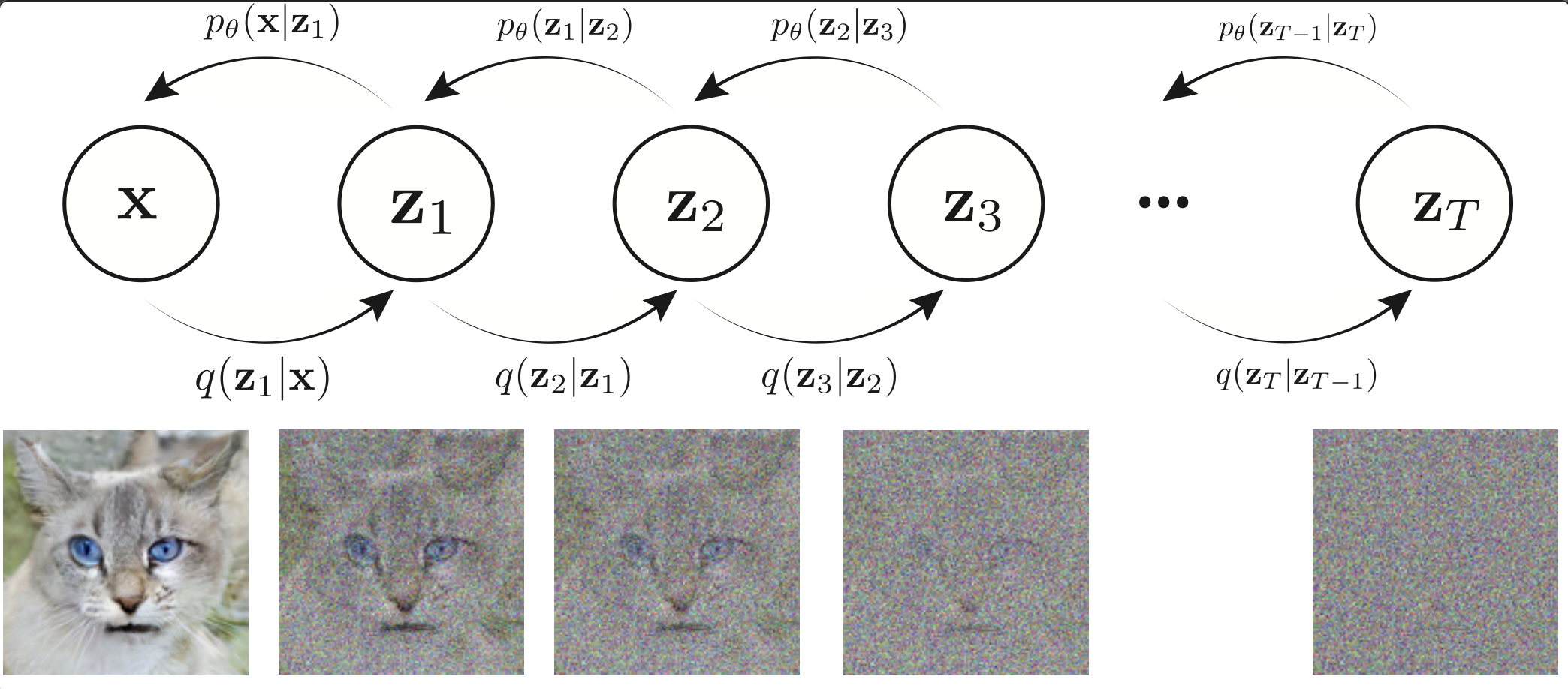
Figure 10: A variational diffusion model adds linear Gaussian noise at each time step, getting a fully Gaussian noise after $T$ latent steps.

Note that our encoder distributions $q_{\phi}(\mathbf{z}_{t}|\mathbf{z}_{t-1})$ in Fig.˜10 are no longer parameterized by $\phi$, as they are completely modeled as Gaussians with defined mean and variance parameters at each timestep. Therefore, in a VDM, we are only interested in learning conditionals $p_{\theta}(\mathbf{z}_{t-1}|\mathbf{z}_{t})$, so that we can simulate new data. After optimizing the VDM, the sampling procedure is as simple as sampling Gaussian noise from $p(\mathbf{z}_{T})$ and iteratively running the denoising transitions $p_{\theta}(\mathbf{z}_{t-1}|\mathbf{z}_{t})$ for $T$ steps to generate a novel $\mathbf{x}$.

Connecting diffusion models with ELBO.

Since in VDMs, the latent variables $\mathbf{z}$ has the same dimensionality as the input, we represent them as $\mathbf{x}_{i}$ with the input data sample as $\mathbf{x}_{0}$. We can now resume from the log likelihood relation with ELBO as (see [Luo, 2022]):

$$\log p(\mathbf{x}) \geq\mathbb{E}_{q(\mathbf{x}_{1:T}|\mathbf{x}_{0})}\left[log\frac{p(\mathbf{x}_{0:T})}{q(\mathbf{x}_{1:T}|\mathbf{x}_{0})}\right]$$ (33)

$$=\underbrace{\mathbb{E}_{q(\mathbf{x}_{1}|\mathbf{x}_{0})}[\log p_{\theta}(\mathbf{x}_{0}|\mathbf{x}_{1})]}_{\text{reconstruction term}}-\underbrace{D_{KL}(q(\mathbf{x}_{T}|\mathbf{x}_{0})||p(\mathbf{x}_{T}))}_{\text{prior matching term}}-\sum_{t=2}^{T}\underbrace{\mathbb{E}_{q(\mathbf{x}_{t}|\mathbf{x}_{0})}[D_{KL}(q(\mathbf{x}_{t-1}|\mathbf{x}_{t},\mathbf{x}_{0})\;||\;p_{\theta}(\mathbf{x}_{t-1}|\mathbf{x}_{t}))].}_{\text{denoising matching term}}$$ (34)

Each term in this formulation has an elegant interpretation:

1. The first term can be interpreted as a reconstruction term and can be approximated and optimized using a Monte Carlo estimate

2. The second term is a distance metric that tells how close the noisy version of the input $\mathbf{x}_{0}$ to the standard Gaussian prior $p(\mathbf{x}_{T})$.

While HVAEs and diffusion models are distinct in their methodologies and approaches to generative modeling, they share the common goal of learning complex data distributions. Their differences in hierarchical structures and generation processes provide unique strengths that, when combined, could lead to more advanced and capable generative models.

5.2 Energy-based models (EBM)

Another similar approach is energy-based modeling, in which a distribution is learned as an arbitrarily flexible energy function that is then normalized. EBMs are much less restrictive in functional form: instead of specifying a normalized probability, they only specify an unnormalized non-negatvive function of the form:

$$p_{\theta}(\mathbf{x})=\frac{\exp(f_{\theta}(\mathbf{x}))}{Z_{\theta}}\text{\; where \;}Z_{\theta}=\int\exp(f_{\theta}(\mathbf{x}))d\mathbf{x}$$ (35)

denotes the normalizing constant to ensure $\int p_{\theta}(\mathbf{x})d\mathbf{x}=1$. $f_{\theta}$ (the negative of the function $-f_{\theta}$ is the energy) is a nonlinear regression function with parameters $\theta$. $Z_{\theta}$ is constant wrt to $\mathbf{x}$ and depends only on the parameters $\theta$. One way to learn such a distribution is by maximizing the likelihood. However, this requires computing the normalization constant $Z_{\theta}$ which is intractable for complex energy functions.

With EBMs, we can side step such intractable computation by estimating the gradient of the log-likelihood using MCMC methods, which implicitly allows likelihood maximization with gradient ascent [Younes, 2000]. Another important property of EBMs is that even though we cannot compute the likelihood of a sample, we can report the relative importance of any sample. This could be beneficial for many applications like object recognition, sequence labeling or image restoration. Given two samples $\mathbf{x}$ and $\mathbf{x}^{\prime}$, the relative importance is the ratio:

$$\frac{p_{\theta}(\mathbf{x})}{p_{\theta}(\mathbf{x}^{\prime})}=\frac{{\exp(f_{\theta}(\mathbf{x}))}/{Z_{\theta}}}{{\exp(-f_{\theta}(\mathbf{x}^{\prime}))}/{Z_{\theta}}}=\frac{\exp(f_{\theta}(\mathbf{x}))}{\exp(-f_{\theta}(\mathbf{x}^{\prime}))}=\exp(f_{\theta}(\mathbf{x})-f_{\theta}(\mathbf{x}^{\prime})).$$ (36)

Since the normalizing constant cancels out in the above ratio, we only need to deal with the $\exp f_{\theta}(\cdot)$ terms which are tractable. In the next section, we see how MCMC methods can be used to train and sample from EBMs.

Contrastive Divergence algorithm.

Intuitively, one can maximize the likelihood (35) by increasing the numerator and decreasing the denominator. The contrastive divergence algorithm Hinton [2002] works on this contrastive idea. To maximize the log-likelihood, we optimize the parameters $\theta$. This requires computing the gradient wrt $\theta$ which has the form:

$$\nabla_{\theta}\log p_{\theta}(\mathbf{x})=\nabla_{\theta}\log(\exp(f_{\theta}(\mathbf{x}))/{Z_{\theta}}) =\nabla_{\theta}f_{\theta}(\mathbf{x})-\nabla_{\theta}\log Z_{\theta}$$ (37)

$$=\nabla_{\theta}f_{\theta}(\mathbf{x})-\frac{\nabla_{\theta}Z_{\theta}}{Z_{\theta}}$$ (38)

$$=f_{\theta}(\mathbf{x})-\frac{1}{Z_{\theta}}\nabla_{\theta}\int\exp(f_{\theta}(\mathbf{x}))d\mathbf{x}$$ (39)

$$=f_{\theta}(\mathbf{x})-\frac{1}{{{Z_{\theta}}}}\int\exp(f_{\theta}(\mathbf{x}))\nabla_{\theta}f_{\theta}(\mathbf{x})d\mathbf{x}$$ (40)

$$=f_{\theta}(\mathbf{x})-\int\frac{\exp(f_{\theta}(\mathbf{x}))}{Z_{\theta}}\nabla_{\theta}f_{\theta}(\mathbf{x})d\mathbf{x}\leftarrow\text{the ratio is a pdf $p_{\theta}(\mathbf{x})$}$$ (41)

$$=f_{\theta}(\mathbf{x})-\mathbb{E}_{\mathbf{x}}[\nabla_{\theta}f_{\theta}(\mathbf{x})]$$ (42)

$$=f_{\theta}(\mathbf{x})-\nabla_{\theta}f_{\theta}(\mathbf{x}_{\text{sample}})\leftarrow\text{one-sample estimate}$$ (43)

The expectation term in Eq.˜42 can be approximated by Monte Carlo estimation. Equation˜43 is a one sample estimate of this expectation. One can sample $\mathbf{x}_{\text{sample}}\sim\exp f(\mathbf{x}_{\text{sample}})/Z_{\theta}$ from the model $p_{\theta}$ and take step in the direction given by the gradient $\nabla\exp(f_{\theta}(\mathbf{x})-f_{\theta}(\mathbf{x}_{\text{sample}}))$ making training data more likely than a typical sample from the model. But the main question remains, how do we sample $\mathbf{x}_{\text{sample}}$? This is where MCMC methods comes into play.

5.2.1 MCMC methods for sampling from EBMs

EBMs are extremely flexible in the way $f_{\theta}$ can be chosen. There is practically no restriction on the choice of $f_{\theta}$. This means, you can plug-in whatever architecture you want to model the data. However, the problem is that sampling from $p_{\theta}(\mathbf{x})$ is very hard. Generating new samples could be computationally very expensive from an EBM. The reason is that evaluating and optimizing likelihood $p_{\theta}(\mathbf{x})$ is hard (i.e., learning is hard). Even if you train your model $p_{\theta}$, sampling would require finding the normalization constant $Z_{\theta}$, which is intractable. This is because fundamentally the numerical cost to compute $Z_{\theta}$ scales exponentially with the number of dimensions of $\mathbf{x}$.

To optimize the log-likelihood form from Eq.˜43, we would like to pick samples $\mathbf{x}_{\text{sample}}$ that represents the underlying data distribution. This can be achieved by using iterative algorithms. At each iteration, we can perform MCMC iterative sampling to obtain the sample $\mathbf{x}_{\text{sample}}$ which can be used to evaluate Eq.˜43. We discuss two important MCMC algorithms below.

Metropolis-Hastings MCMC

We can use Metropolis-Hastings MCMC sampling algorithm which is an iterative method:

• Initialize a random sample $\mathbf{x}_{0}$ at $t=0$

• Repeat the process for $t=0,1,2,\cdots,T-1$

  $\mathbf{x}^{\prime}=\mathbf{x}^{t}+\text{noise}$

  If $f(\mathbf{x}^{\prime})>f(\mathbf{x}^{t})$ then $\mathbf{x}^{t+1}=\mathbf{x}^{\prime}$

  else let $f(\mathbf{x}^{t+1})=\mathbf{x}^{\prime}$ with probability $\exp(f_{\theta}(\mathbf{x}^{t})-f_{\theta}(\mathbf{x}^{\prime}))$

Here the noise term could be any perturbation that can be added to the data sample. Note that, unlike standard MH algorithm—where the samples rejected if they fall below the accepted probability—we accept samples which have lower probability than the acceptance ratio. This is because we want to keep sampling the space. We simply ensure tehe sample is accepted with the lower probaility. In theory, MCMC sampling works but it can take quite a long time to converge.

Unadjusted Langevin MCMC

Slightly better version of MCMC sampling is using Langevin dynamics. Sampling using the unadjusted Langevin MCMC algorithm (ULA) works as follows:

• Initialize a random sample $\mathbf{x}^{0}\sim p(\mathbf{x})$ at $t=0$

• Repeat for $t=0,1,2,\ldots,T-1$

  $\mathbf{z}^{t}\sim\mathcal{N}(0,I)$

  $\mathbf{x}^{t+1}=\mathbf{x}^{t}+\epsilon\nabla_{x}\log p_{\theta}(\mathbf{x})|_{\mathbf{x}=\mathbf{x}^{t}}+\sqrt{2\epsilon}\mathbf{z}^{t}$

Here $\epsilon$ is the step size. Note that ULA has no rejection step. The samples are perturbed with a noise $\mathbf{z}_{t}$ and the new sample is accepted. However, in theory this algorithm can only converge if the step size $\epsilon$ is small. But this can slow down the convergence dramatically. At least, the perturbation is informed thanks to the $\nabla_{x}p_{\theta}(\mathbf{x})|_{\mathbf{x}=\mathbf{x}_{t}}$ term. In MH algorithm, the noise added could be any random perturbation. ULA has many noticeable properties:

• $\mathbf{x}^{T}$ converges to a sample from $p_{\theta}(\mathbf{x})$ as $T\rightarrow\infty$ and the step size $\epsilon\rightarrow 0$.

• ULA has better convergence compared to MH MCMC because now the exploration is informed thanks to the $\nabla_{\mathbf{x}}\log p_{\theta}(\mathbf{x})$ term.

• $\nabla_{\mathbf{x}}\log p_{\theta}(\mathbf{x})=\nabla_{x}f_{\theta}(\mathbf{x})$ for continuous energy models, which implies that the normalization term is completely gone.

There are still issues with this approach. Sampling converges slowly in higher dimensional spaces and is thus very expensive, yet we need sampling in every iteration in contrastive divergence. For example, every time we need to sample to solve Eq.˜43, we need to run (say 1000) large number of iterations of an MCMC algorithm to generate a valid sample that follows the underlying distribution $p_{\theta}$.Yet, we need sampling at each iteration in contrastive divergence. Gao et al. [2021] propose to train energy-based models by diffusion recovery likelihood where long-run MCMC samples from the conditional distributions do not diverge and still represent realistic images. This allows them to accurately estimate the normalized density of data even for high-dimensional datasets.

Training without sampling.

To avoid such expensive sampling procedures one can use training methods that does not require sampling. Score matching [Hyvärinen, 2005, Song and Ermon, 2020a, Song et al., 2019] and noise contrast estimation [Gutmann and Hyvärinen, 2010] algorithms are such methods that does not require sampling for training. We will not delve much into these methods. However, we will briefly looking score-based models in the next section as they require sampling to generate new samples where MCMC methods shine again.

5.3 Sampling score-based generative models

So far we have been talking about energy-based models which suffer from expensive sampling during the training stage. Score-based models can help avoid this sampling step altogether from the training stage. Score-based generative models are highly related to EBMs; instead of learning to model the energy function itself, they learn the score of the energy-based model as a neural network.

Starting from Eq.˜35:

$$p_{\theta}(\mathbf{x}) =\frac{\exp f_{\theta}(\mathbf{x})}{Z_{\theta}}$$ (44)

$$\log p_{\theta}(\mathbf{x}) =f_{\theta}(\mathbf{x})-\log Z_{\theta}$$ (45)

$$\nabla_{\mathbf{x}}\log p_{\theta}(\mathbf{x}) =\nabla_{\mathbf{x}}f_{\theta}(\mathbf{x})-\underbrace{\nabla_{\mathbf{x}}\log Z_{\theta}}_{=0}$$ (46)

$$\nabla_{\mathbf{x}}\log p_{\theta}(\mathbf{x}) =\nabla_{\mathbf{x}}f_{\theta}(\mathbf{x})=\mathbf{s}_{\theta}(\mathbf{x})$$ (47)

Taking the gradient of the log-likelihood wrt to $\mathbf{x}$ renders the summand on the RHS to zero since the normalization constant (aka the partion function) $Z_{\theta}$ only depends on $\theta$. The $\mathbf{s}_{\theta}(\mathbf{x})$ is the score function.

The score $\mathbf{s}_{\theta}(\mathbf{x})$ provides an alternative view of the original function where you are looking at things from the perspective of the gradient instead of the perspective of the likelihood itself. The key observation here is that the score is independent of the normalization constant (aka the partion function) $Z_{\theta}$.

What does the score function represent? For every $\mathbf{x}$, taking the gradient of its log likelihood with respect to $\mathbf{x}$ essentially describes what direction in data space to move in order to further increase its likelihood. Intuitively, the score function defines a vector field over the entire data space, pointing towards the modes.

Some efficient MCMC methods, such as Langevin MCMC or Hamiltonian MC Radford [2011], make use of the fact that the gradient of the log-probability wrt $\mathbf{x}$ (a.k.a score) is equal to the (negative) gradient of the energy, therefore easy to calculate.

By learning the score function of the true data distribution, we can generate samples by starting at any arbitrary point in the same space and iteratively following the score until a mode is reached. This sampling procedure is known as Langevin dynamics, and is mathematically described as:

$$\mathbf{x}_{i+1}=\mathbf{x}_{i}+c\nabla\log p(\mathbf{x}_{i})+\sqrt{2c}\epsilon$$ (48)

Collectively, learning to represent a distribution as a score function and using it to generate samples through MCMC techniques, such as Langevin dynamics, is known as Score-based Generative Modeling [Song et al., 2021, Song and Ermon, 2020a, b].

6 Conclusion

MCMC methods offer a unified framework for sampling from complex probability distributions, addressing a common challenge across the domains of rendering, generative modeling, and optimization. Significant research efforts have been dedicated to identifying the conceptual bridge between these interconnected fields.

However, there are a number of challenges that need to be addressed. For example, the chain constructed by the Ordinary Metropolis Hastings algorithm is not only invariant, but even reversible with respect to the target distribution. This invariance property, which is necessary for usage in Monte Carlo sampling, highly restricts our choice of processes, which we can use for state space exploration. That is, even when we have a process at hand, which is able to explore our given state space in a favorable manner, we cannot use it for Monte Carlo sampling, unless it is invariant. Reversibility is an even stronger condition. While it yields certain useful spectral properties of the process, it also slows down mixing and convergence to equilibrium. Reversible processes show backtracking behavior where the processes frequently revisit previously visited states before reaching unexplored areas, thereby, slowing down the convergence. Another challenge with designing MCMC algorithms is that the highly correlated Markov chains can cause excessive local exploration which in rendering are visible as overly bright pixels. To avoid this issue, MCMC algorithms should discover other contributing areas by globally discovering the paths away from the current path. All existing algorithms [Veach and Guibas, 1997, Luan et al., 2020, Li et al., 2015, Pantaleoni, 2017, Bitterli et al., 2017, Bitterli and Jarosz, 2019] are based Metropolis-Hastings which inherits its slower convergence due to the reversibility property. Recently, Holl et al. [2024] introduced a continuous time Markov framework that is based on the restore algorithm [Wang et al., 2021]. Their framework adjusts an arbitrary Markov chain for Monte Carlo integration to the graphics community. Especially, they introduced a rejection-free and target density sensitive way to deal with global discovery. They generalized the idea presented in Wang et al. [2021] and extended it for light transport rendering problems. Given the surge in generative models, this work provides a solid foundational framework that can be leveraged to establish direct connections between diffusion models in generative modeling, physically based rendering and SGD-based optimization algorithms.

We believe that this course will equip participants with the knowledge to bridge the gaps between physically based rendering and vision-based generative modeling more effectively. We are excited about how understanding MCMC will enable participants to recognize the common probabilistic foundation underlying diverse applications. This insight will enhance their ability to apply learned concepts across different domains.

7 Speakers

Gurprit Singh

is a senior researcher at the Max Planck Institute (MPI) for Informatics, where he is currently leading the sampling & rendering group. His research interests are in Markov Chain Monte Carlo (MCMC), diffusion models, noise correlations and Monte Carlo sampling for physically based (forward/inverse) rendering. He has published his research in the top-tier conferences like SIGGRAPH (North America/Asia), NeurIPS, ECCV, Eurographics. His current focus is on bridging the gap between physically based rendering and generative AI using the powerful machinery of MCMC methods.
Email: gsingh@mpi-inf.mpg.de   Webpage: https://sampling.mpi-inf.mpg.de/

Wenzel Jakob

is an associate professor leading the Realistic Graphics Lab at EPFL’s School of Computer and Communication Sciences. Wenzel has received the ACM SIGGRAPH Significant Researcher award, the Eurographics Young Researcher Award, and an ERC Starting Grant. His group develops the Mitsuba renderer Jakob et al. [2022], a research-oriented rendering system, and he has co-authored the third and fourth editions of Physically Based Rendering: From Theory To Implementation Pharr et al. [2023].
Email: wenzel.jakob@epfl.ch   Webpage: https://rgl.epfl.ch/people/wjakob

Appendix A Code snippets

Listing 3: Python example

⬇

# Brownian motion

import numpy as np

import matplotlib.pyplot as plt

# Function to simulate Brownian motion

def brownian_motion(num_steps, step_size):

# Initialize position at the origin

position = np.zeros(2)

positions = [position.copy()]

# Iterate through each step

for _ in range(num_steps):

# Generate random displacement for each dimension

displacement = np.random.normal(0, step_size, size=2)

# Update position

position += displacement

# Store the updated position

positions.append(position.copy())

return np.array(positions)

# Number of steps and step size

num_steps = 1000

step_size = 0.1

# Simulate Brownian motion

positions = brownian_motion(num_steps, step_size)

# Plot the Brownian motion trajectory

plt.plot(positions[:, 0], positions[:, 1], lw=1)

plt.title(’2D Brownian Motion’)

plt.xlabel(’X’)

plt.ylabel(’Y’)

plt.show()

Listing 4: Python example

⬇

# Unadjusted Langevin Monte Carlo sampling

import numpy as np

import matplotlib.pyplot as plt

def target_log_prob(x):

Example target distribution: standard normal distribution

def grad_target_log_prob(x):

# Gradient of the log of the target distribution: standard normal distribution

return -x

def langevin_monte_carlo(num_samples, dim, step_size, burn_in):

samples = np.zeros((num_samples, dim))

current_sample = np.random.randn(dim) # Initialize with a random sample

for i in range(num_samples + burn_in):

grad_log_prob = grad_target_log_prob(current_sample)

noise = np.random.randn(dim)

next_sample = current_sample + 0.5 * step_size * grad_log_prob + np.sqrt(step_size) * noise

# Accept the next sample

current_sample = next_sample

if i >= burn_in:

samples[i - burn_in] = current_sample

return samples

# Parameters

num_samples = 10000 # Number of samples to generate

dim = 2 # Dimension of the target distribution

step_size = 0.1 # Step size for the Langevin dynamics

burn_in = 100 # Number of burn-in steps

# Generate samples

samples = langevin_monte_carlo(num_samples, dim, step_size, burn_in)

# Create subplots

fig, axs = plt.subplots(1, 1, figsize=(5, 5))

# Plot Brownian motion trajectory

# axs[0].plot(positions[:, 0], positions[:, 1], lw=1)

axs.scatter(samples[:, 0], samples[:, 1], s=0.5)

axs.set_title(’LMC’)

axs.set_xlabel(’X’)

axs.set_ylabel(’Y’)

axs.set_xlim(-3, 3)

axs.set_ylim(-3, 3)

# axs.grid(True)

axs.set_aspect(1)

plt.tight_layout()

plt.show()

Listing 5: Python example

⬇

# Unadjusted Hamiltonian Monte Carlo

import numpy as np

import matplotlib.pyplot as plt

# Define the target distribution (posterior) - For example, a Gaussian distribution

def log_prob(theta):

"""Returns the log of the target distribution (up to a constant)"""

return -0.5 * np.sum(theta ** 2)

# Gradient of the log-probability

def grad_log_prob(theta):

"""Returns the gradient of the log-probability"""

return -theta

# Hamiltonian Monte Carlo Sampling

def hmc(log_prob, grad_log_prob, initial_theta, n_samples, step_size, n_leapfrog):

"""

log_prob: function to compute log-probability of the target distribution

grad_log_prob: function to compute the gradient of the log-probability

initial_theta: initial value of parameters (starting point)

n_samples: number of samples to generate

step_size: step size for the leapfrog integrator

n_leapfrog: number of leapfrog steps in the simulation

"""

samples = []

current_theta = initial_theta

current_log_prob = log_prob(current_theta)

for _ in range(n_samples):

% # Sample a random momentum (p) from a normal distribution

current_p = np.random.normal(0, 1, size=current_theta.shape)

initial_p = current_p

% # Hamiltonian dynamics step (Leapfrog integrator)

theta = np.copy(current_theta)

p = np.copy(current_p)

% # Half-step update of momentum

p -= 0.5 * step_size * grad_log_prob(theta)

% # Full-step updates of position (theta) and momentum (p)

for _ in range(n_leapfrog):

# Update theta

theta += step_size * p

% # Update momentum (except the last iteration)

if _ < n_leapfrog - 1:

p -= step_size * grad_log_prob(theta)

% # Final half-step update of momentum

p -= 0.5 * step_size * grad_log_prob(theta)

% # Negate the momentum to make the proposal symmetric

p = -p

% # Compute Hamiltonian at the start and end of the trajectory

current_H = -current_log_prob + 0.5 * np.sum(initial_p ** 2)

proposed_H = -log_prob(theta) + 0.5 * np.sum(p ** 2)

% # Metropolis acceptance criterion

if np.random.uniform(0, 1) < np.exp(current_H - proposed_H):

current_theta = theta

current_log_prob = log_prob(current_theta)

samples.append(current_theta)

return np.array(samples)

# Generate samples using HMC

samples = hmc(log_prob, grad_log_prob, initial_theta, n_samples, step_size, n_leapfrog)

References

- Betancourt [2018] M. Betancourt. A conceptual introduction to hamiltonian monte carlo, 2018. URL https://arxiv.org/abs/1701.02434.
- Bitterli and Jarosz [2019] B. Bitterli and W. Jarosz. Selectively Metropolised Monte Carlo light transport simulation. ACM Transactions on Graphics (Proceedings of SIGGRAPH Asia), 38(6), Nov. 2019. doi: 10.1145/3355089.3356578.
- Bitterli et al. [2017] B. Bitterli, W. Jakob, J. Novák, and W. Jarosz. Reversible jump metropolis light transport using inverse mappings. ACM Transactions on Graphics, 37(1), Oct. 2017. doi: 10.1145/3132704.
- Chen et al. [2016] C. Chen, D. Carlson, Z. Gan, C. Li, and L. Carin. Bridging the Gap between Stochastic Gradient MCMC and Stochastic Optimization. In A. Gretton and C. C. Robert, editors, Proceedings of the 19th International Conference on Artificial Intelligence and Statistics, volume 51 of Proceedings of Machine Learning Research, pages 1051–1060, Cadiz, Spain, 09–11 May 2016. PMLR. URL https://proceedings.mlr.press/v51/chen16c.html.
- Gao et al. [2021] R. Gao, Y. Song, B. Poole, Y. N. Wu, and D. P. Kingma. Learning energy-based models by diffusion recovery likelihood, 2021. URL https://arxiv.org/abs/2012.08125.
- Gutmann and Hyvärinen [2010] M. Gutmann and A. Hyvärinen. Noise-contrastive estimation: A new estimation principle for unnormalized statistical models. In Y. W. Teh and M. Titterington, editors, Proceedings of the Thirteenth International Conference on Artificial Intelligence and Statistics, volume 9 of Proceedings of Machine Learning Research, pages 297–304, Chia Laguna Resort, Sardinia, Italy, 13–15 May 2010. PMLR. URL https://proceedings.mlr.press/v9/gutmann10a.html.
- Hairer et al. [2013] E. Hairer, C. Lubich, and G. Wanner. Geometric Numerical Integration: Structure-Preserving Algorithms for Ordinary Differential Equations. Springer Series in Computational Mathematics. Springer Berlin Heidelberg, 2013. ISBN 9783662050187. URL https://books.google.cz/books?id=cPTxCAAAQBAJ.
- Hinton [2002] G. E. Hinton. Training products of experts by minimizing contrastive divergence. Neural Comput., 14(8):1771–1800, aug 2002. ISSN 0899-7667. doi: 10.1162/089976602760128018. URL https://doi.org/10.1162/089976602760128018.
- Ho et al. [2020] J. Ho, A. Jain, and P. Abbeel. Denoising diffusion probabilistic models. In Proceedings of the 34th International Conference on Neural Information Processing Systems, NIPS ’20, Red Hook, NY, USA, 2020. Curran Associates Inc. ISBN 9781713829546.
- Holl et al. [2024] S. Holl, H.-P. Seidel, and G. Singh. Jump restore light transport, 2024. URL https://arxiv.org/abs/2409.07148.
- Hyvärinen [2005] A. Hyvärinen. Estimation of non-normalized statistical models by score matching. Journal of Machine Learning Research, 6(24):695–709, 2005. URL http://jmlr.org/papers/v6/hyvarinen05a.html.
- Ivo et al. [2019] K. Ivo, P. Vévoda, P. Grittmann, T. Skřivan, P. Slusallek, and J. Křivánek. Optimal multiple importance sampling. ACM Transactions on Graphics (Proceedings of SIGGRAPH 2019), 38(4):37:1–37:14, July 2019. doi: 10.1145/3306346.3323009.
- Jakob et al. [2022] W. Jakob, S. Speierer, N. Roussel, M. Nimier-David, D. Vicini, T. Zeltner, B. Nicolet, M. Crespo, V. Leroy, and Z. Zhang. Mitsuba 3 renderer, 2022. URL https://mitsuba-renderer.org.
- Kelemen et al. [2002] C. Kelemen, L. Szirmay-Kalos, G. Antal, and F. Csonka. A simple and robust mutation strategy for the Metropolis light transport algorithm. Computer Graphics Forum, 21(3):531–540, 2002.
- Kingma et al. [2023] D. P. Kingma, T. Salimans, B. Poole, and J. Ho. Variational diffusion models, 2023. URL https://arxiv.org/abs/2107.00630.
- Kollig and Keller [2002] T. Kollig and A. Keller. Efficient bidirectional path tracing by randomized quasi-Monte Carlo integration. Springer, 2002.
- Leimkuhler and Reich [2005] B. Leimkuhler and S. Reich. Simulating Hamiltonian Dynamics. Cambridge Monographs on Applied and Computational Mathematics. Cambridge University Press, 2005.
- Li et al. [2015] T.-M. Li, J. Lehtinen, R. Ramamoorthi, W. Jakob, and F. Durand. Anisotropic Gaussian Mutations for Metropolis Light Transport through Hessian-Hamiltonian Dynamics. ACM Trans. Graph., 34(6), nov 2015. ISSN 0730-0301. doi: 10.1145/2816795.2818084. URL https://doi.org/10.1145/2816795.2818084.
- Luan et al. [2020] F. Luan, S. Zhao, K. Bala, and I. Gkioulekas. Langevin Monte Carlo Rendering with Gradient-based Adaptation. ACM Trans. Graph., 39(4), 2020. URL https://dl.acm.org/doi/abs/10.1145/3386569.3392382.
- Luo [2022] C. Luo. Understanding Diffusion Models: A Unified Perspective, 2022. URL https://arxiv.org/abs/2208.11970.
- Pantaleoni [2017] J. Pantaleoni. Charted metropolis light transport. ACM Transactions on Graphics, 36(4):1–14, July 2017. ISSN 1557-7368. doi: 10.1145/3072959.3073677. URL http://dx.doi.org/10.1145/3072959.3073677.
- Pharr et al. [2023] M. Pharr, W. Jakob, and G. Humphreys. Physically based rendering: From theory to implementation. Morgan Kaufmann, 2023. URL https://www.pbr-book.org/.
- Radford [2011] N. Radford. Mcmc using hamiltonian dynamics. May 2011. doi: 10.1201/b10905. URL https://arxiv.org/pdf/1206.1901.
- Roberts and Stramer [2002] G. O. Roberts and O. Stramer. Langevin Diffusions and Metropolis-Hastings Algorithms. Method. Comput. Appl. Prob., 4(4):337–357, dec 2002. ISSN 1387-5841. doi: 10.1023/A:1023562417138. URL https://doi.org/10.1023/A:1023562417138.
- Sohl-Dickstein et al. [2015] J. Sohl-Dickstein, E. A. Weiss, N. Maheswaranathan, and S. Ganguli. Deep Unsupervised Learning using Nonequilibrium Thermodynamics, 2015. URL https://arxiv.org/abs/1503.03585.
- Song and Ermon [2020a] Y. Song and S. Ermon. Generative modeling by estimating gradients of the data distribution, 2020a. URL https://arxiv.org/abs/1907.05600.
- Song and Ermon [2020b] Y. Song and S. Ermon. Improved techniques for training score-based generative models. In Proceedings of the 34th International Conference on Neural Information Processing Systems, NIPS ’20, Red Hook, NY, USA, 2020b. Curran Associates Inc. ISBN 9781713829546.
- Song et al. [2019] Y. Song, S. Garg, J. Shi, and S. Ermon. Sliced score matching: A scalable approach to density and score estimation, 2019. URL https://arxiv.org/abs/1905.07088.
- Song et al. [2021] Y. Song, J. Sohl-Dickstein, D. P. Kingma, A. Kumar, S. Ermon, and B. Poole. Score-Based Generative Modeling through Stochastic Differential Equations, 2021. URL https://arxiv.org/abs/2011.13456.
- Veach [1998] E. Veach. Robust Monte Carlo Methods for Light Transport Simulation. PhD thesis, Stanford University, Stanford, CA, USA, 1998. AAI9837162.
- Veach and Guibas [1995] E. Veach and L. J. Guibas. Optimally combining sampling techniques for Monte Carlo rendering. In Proceedings of the 22nd annual conference on Computer graphics and interactive techniques, SIGGRAPH ’95, pages 419–428. ACM, 1995.
- Veach and Guibas [1997] E. Veach and L. J. Guibas. Metropolis light transport. In Proceedings of the 24th Annual Conference on Computer Graphics and Interactive Techniques, SIGGRAPH ’97, page 65–76, USA, 1997. ACM Press/Addison-Wesley Publishing Co. ISBN 0897918967. doi: 10.1145/258734.258775. URL https://doi.org/10.1145/258734.258775.
- Wang et al. [2021] A. Q. Wang, M. Pollock, G. O. Roberts, and D. Steinsaltz. Regeneration-enriched markov processes with application to monte carlo. The Annals of Applied Probability, 31(2), Apr. 2021. ISSN 1050-5164. doi: 10.1214/20-aap1602. URL http://dx.doi.org/10.1214/20-AAP1602.
- Welling and Teh [2011] M. Welling and Y. W. Teh. Bayesian learning via stochastic gradient langevin dynamics. In Proceedings of the 28th International Conference on International Conference on Machine Learning, ICML’11, page 681–688, Madison, WI, USA, 2011. Omnipress. ISBN 9781450306195. URL https://icml.cc/2011/papers/398_icmlpaper.pdf.
- Younes [2000] L. Younes. On the convergence of markovian stochastic algorithms with rapidly decreasing ergodicity rates. Stochastics and Stochastics Reports, 65, 04 2000. doi: 10.1080/17442509908834179.