MEC³O: Multi-Expert Consensus for Code Time Complexity Prediction

Abstract

Predicting the complexity of source code is essential for software development and algorithm analysis. Recently, Baik et al. (2025) introduced CodeComplex for code time complexity prediction. The paper shows that LLMs without fine-tuning struggle with certain complexity classes. This suggests that no single LLM excels at every class, but rather each model shows advantages in certain classes. We propose MEC³O, a multi-expert consensus system, which extends the multi-agent debate frameworks. MEC³O assigns LLMs to complexity classes based on their performance and provides them with class-specialized instructions, turning them into experts. These experts engage in structured debates, and their predictions are integrated through a weighted consensus mechanism. Our expertise assignments to LLMs effectively handle Degeneration-of-Thought, reducing reliance on a separate judge model, and preventing convergence to incorrect majority opinions. Experiments on CodeComplex show that MEC³O outperforms the open-source baselines, achieving at least 10% higher accuracy and macro-F1 scores. It also surpasses GPT-4o-mini in macro-F1 scores on average and demonstrates competitive on-par F1 scores to GPT-4o and GPT-o4-mini on average. This demonstrates the effectiveness of multi-expert debates and a weighted consensus strategy to generate the final predictions.

envname-P envname#1

MEC³O: Multi-Expert Consensus for Code Time Complexity Prediction

Joonghyuk Hahn, Soohan Lim, Yo-Sub Han, Department of Computer Science, Yonsei University, Seoul, Republic of Korea, {greghahn,aness1219,emmous}@yonsei.ac.kr

1 Introduction

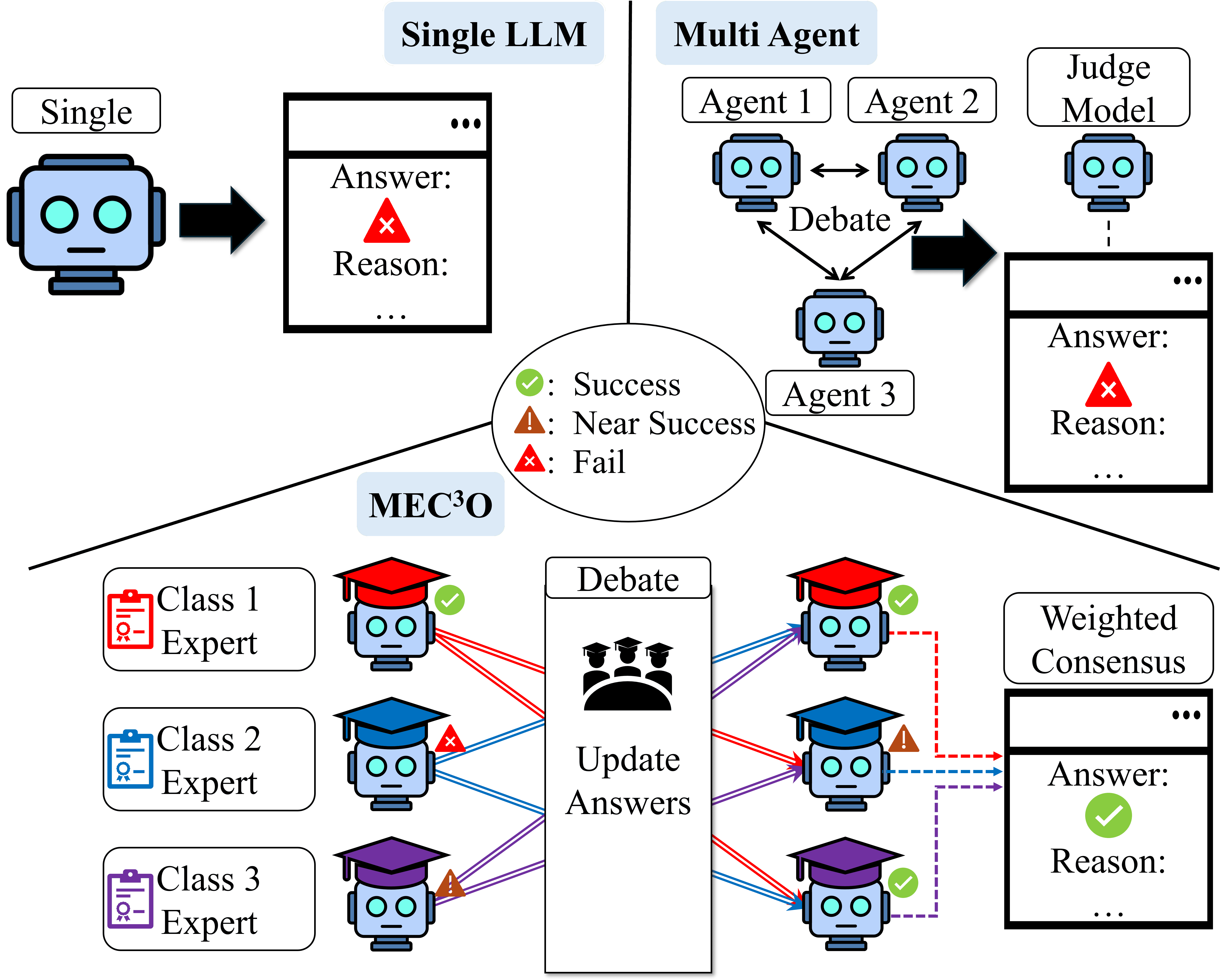
Figure 1: Procedural comparison of Single LLM, multi-agent debate, and MEC³O approaches.

Time complexity prediction of the source code is a fundamental task in software development Sikka et al. (2020) and algorithm analysis Lu et al. (2021); Peng et al. (2021); Wang et al. (2024b), since it affects the scalability and performance of real-world applications. Recent advances in large language models (LLMs) have enabled automatic code completion, bug fixing, and summarization at near-human levels of fluency Bouzenia et al. (2024); Haldar and Hockenmaier (2024); Nam et al. (2024). However, despite the success of single-model paradigms such as GPT-4 OpenAI (2023), they often become locked into a specific line of reasoning, known as ‘Degeneration-of-Thought (DoT)’ Liang et al. (2024). Once a model settles on an initial conclusion, it may fail to reconsider even when encountering contradictory evidence, limiting overall reliability and coverage. This procedural distinction among a single LLM, conventional multi-agent debate, and our proposed MEC³O framework is summarized in Figure 1.

Multi-agent debate or self-reflection strategies(Du et al., 2024; Madaan et al., 2023; Shinn et al., 2023) attempt to address DoT by involving self-refining or multiple agents that challenge each other’s reasoning. However, these solutions rely on a single underlying LLM architecture or lack a clear plan for handling conflicting statements for different models. In some cases, a separate judge model finalizes the outcome, which can overshadow correct but minority opinions. This problem is observed even in conventional majority votes. Consequently, improvements are constrained by whichever mechanism to handle the consensus of debate.

Here, we focus on predicting the time complexity of code snippets in multiple programming languages, such as Java and Python. We define a seven-class categorization scheme: $O(1)$, $O(\log n)$, $O(n)$, $O(n\log n)$, $O(n^{2})$, $O(n^{3})$, and $O(2^{n})$. We observe that a single LLM can perform well on one class and poorly on another, suggesting no single model excels across all classes Baik et al. (2025). We propose MEC³O, a multi-expert consensus system for code time complexity prediction. Our method builds on the premise that no single LLM excels at every class, but rather each model shows comparative advantages in certain classes. MEC³O first uses a small expertise set to identify the LLM that performs the best for each complexity class. That model then receives a class-specific instruction, becoming an expert on that class. After the debate of these experts, MEC³O utilizes a weighted consensus, with each expert’s vote scaled by its proven reliability for its expertise class. This setup resolves DoT by letting specialized experts challenge locked-in errors and avoids relying on a separate judge model.

Empirical results on CodeComplex (Baik et al., 2025) demonstrate that MEC³O outperforms all the baselines, and achieves competitive performance to commercial LLMs such as GPT-4o, GPT-4o-mini, and GPT-o4-mini. We believe these findings suggest that multi-LLM collaboration, guided by class-focused experts and weighted consensus, offers robust performance gains for code complexity prediction and related tasks.

2 Related Works

2.1 LLMs for Code Analysis

Recently, Large Language Models (LLMs) have advanced to code-related tasks such as code generation, debugging, and summarization Ahmed et al. (2024); Coignion et al. (2024); Zhong et al. (2024). They demonstrate remarkable fluency and adaptability, often achieving strong performance without extensive domain-specific fine-tuning Aycock and Bawden (2024); Li et al. (2023); Wang et al. (2023); Wei et al. (2022). However, these models can have biases when handling programming styles or domain elements. In many cases, a single model can be locked into its first reasoning path and fail to revise incorrect inferences, even when new evidence arises Creswell et al. (2023); Shinn et al. (2023). This behavior leads to persistent errors, which can affect code-related tasks that require deeper reasoning or algorithmic understanding.

2.2 Code Time Complexity Prediction

Time complexity prediction has conventionally relied on manual inspection by domain experts Sikka et al. (2020). As the number of code snippets scales in size and sophistication, automated approaches have become increasingly appealing. There exist several benchmark datasets (Sikka et al., 2020; Baik et al., 2025) for this task. CoRCoD Sikka et al. (2020) is the first benchmark dataset with 932 code snippets covering five complexity classes: $O(1)$, $O(\log n)$, $O(n)$, $O(n\log n)$, and $O(n^{2})$. Then, extending CoRCoD, Baik et al. (2025) presented CodeComplex, which consists of 9,800 code snippets of two programming languages, Java and Python, and covers seven complexity classes: $O(1)$, $O(\log n)$, $O(n)$, $O(n\log n)$, $O(n^{2})$, $O(n^{3})$, and $O(2^{n})$. We take CodeComplex to offer a robust testing ground for evaluating how well LLMs generalize across different algorithmic complexities.

2.3 Multi-Agent Debate

Single LLM approaches optimize individual performance Wei et al. (2022); Yao et al. (2023), whereas multi-agent debate systems leverage diverse LLMs for collaborative reasoning by debate and discussions Du et al. (2024); Chen et al. (2024); Liang et al. (2024); Wang et al. (2024a). Basic multi-agent debate frameworks typically involve agents proposing and refuting answers, with final predictions decided by majority vote Du et al. (2024) or a separate judge Liang et al. (2024). Other variants introduce confidence-weighted voting Chen et al. (2024) or a hierarchical debate across groups Wang et al. (2024a). However, these methods often suffer from wrong answer propagation, especially when incorrect majority opinions override correct minority ones. Judge models also risk bias or failure, as they depend on a single LLM for final decisions.

Our work addresses these issues by assigning class-specific expert roles to each agent and using a weighted consensus mechanism that reflects the demonstrated strengths of agents. This design encourages the refinement of answers when they are contradicted by a domain expert, thereby mitigating DoT and reducing the dilution of correct answers. In contrast to previous studies, our framework makes consensus decisions without a separate judge, enhancing robustness and leveraging expert diversity more effectively.

3 Background

We briefly overview the time complexity classes that constitute our prediction targets. Then, we formalize the overall classification problem, including the dataset, class labels, and basic notations. This setup will underpin our multi-agent system described in Section 4.

3.1 Preliminaries

We consider seven time complexity classes as the target labels for code time complexity prediction: $O(1)$, $O(\log n)$, $O(n)$, $O(n\log n)$, $O(n^{2})$, $O(n^{3})$, and $O(2^{n})$, where $n$ is the size of the input to the corresponding code snippet. Below, we briefly describe the classes and explain why we assign expertise at the class level.

Why Class-Level Expertise?​​

Time complexity labels often pose challenges for a single LLM, which may overfit to superficial loop structures or miss recursion patterns, leading to persistent errors. Assigning expertise at the class level and providing class-specific instructions help mitigate these issues by allowing models to focus on complexity patterns they handle the best. For instance, an expert specialized in $O(n\log n)$ can accurately detect sorting algorithms that a general LLM might misinterpret as $O(n)$ or $O(n^{2})$. This targeted expertise reduces errors and improves overall prediction reliability.

Constant ($O(1)$):

Code snippets in this category runs in a constant time to their input size. These code snippets have constant-time operations or immediate return conditions.

Logarithmic $O(\log n)$:

Functions in logarithmic time typically arise in divide-and-conquer scenarios, such as binary search. They involve recognizing patterns that split the input range in half each step.

Linear ($O(n)$):

Linear time patterns are the most common in practice, where a loop processes each element of the input once.

Linearithmic ($O(n\log n)$):

Many efficient sorting algorithms and divide-and-conquer methods fall into this category.

Quadratic ($O(n^{2})$):

Quadratic runtime typically emerges from a nested loop. An expert model for this class can interpret loop bounds and break conditions, and then determine the depth of the nested loop to distinguish the complexity class.

Cubic ($O(n^{3})$):

Nested loops of depth three or cubic matrix operations generally indicate $O(n^{3})$.

Exponential ($O(2^{n})$):

Exponential code snippets arise in backtracking, exhaustive searches, or subsets generation. These show the exponential number of branch factors to the input size.

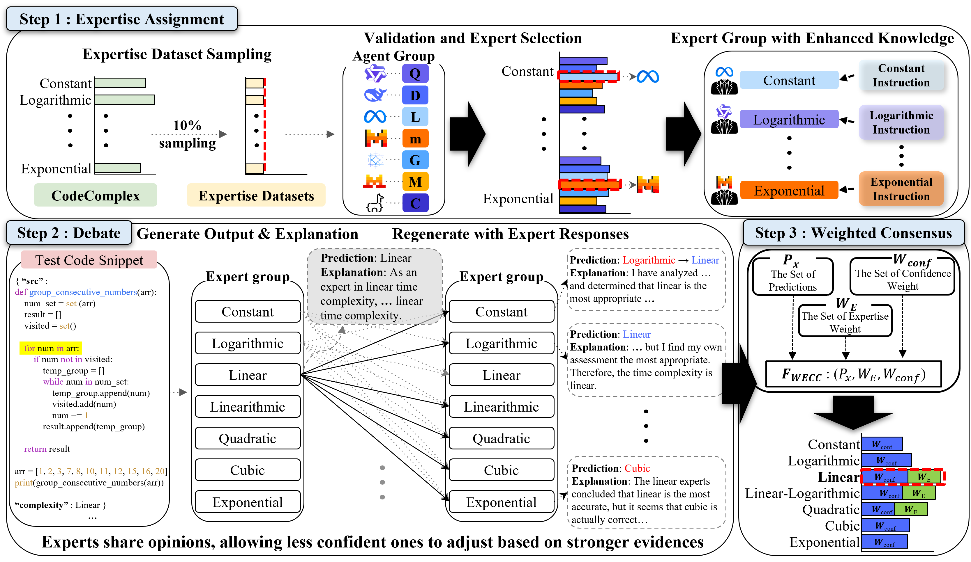
Figure 2: An Overview of MEC³O. Step 1: Expertise assignments via model selection and expertise assignments by class-specific instructions. Step 2: Multi-expert debates. Step 3: Weighted consensus strategy for the final prediction. Appendix O provides a workflow of the debate process.

3.2 Problem Setup

Let $\mathcal{X}$ be the set of code snippets and $\mathcal{C}$ be the set of time complexity classes defined in Section 3.1. Our goal is to optimize the reasoning of an LLM $\mathsf{LLM}$, which maps each code snippet $x\in\mathcal{X}$ to a complexity label $c\in\mathcal{C}$ along with its opinion $o\in\mathcal{O}$:

$$\mathsf{LLM}:\mathcal{X}\rightarrow(\mathcal{C},\mathcal{O}).$$

In our multi-expert framework, we have a set $M$ of candidate LLMs, each assigned as an expert for a specific complexity class:

$$\{M_{c_{1}},\ldots,M_{c_{7}}\}.$$

For a code snippet $x$, each expert receives a class-specific instructions $I_{\mathrm{ex}}$:

$$\mathsf{LLM}(x,I_{\mathrm{ex}})=(p_{i},o_{i})\text{ where }p_{i}\in\mathcal{C}\text{ and }o_{i}\in\mathcal{O}.$$

The experts engage in structured debates, and their outputs are aggregated using a weighted consensus mechanism to determine the final complexity prediction $\hat{c}$. This design addresses the limitation of a single model locking into an incorrect prediction, ensuring that the final decision is determined by experts in their respective complexity classes. The full methodology is described in Section 4.

4 Method

MEC³O (Multi-Experts Consensus for Code Complexity Prediction) coordinates multiple open-source LLMs into specialized experts for different complexity classes, conducts a debate phase to refine opinions, and aggregates final predictions using weighted consensus. Our system draws a clear line between an opinion–the explanatory outputs an experts provides–and a prediction–the final discrete label an expert offers once debate is complete.

4.1 Overall Framework

Let $\{M_{1},M_{2},\ldots,M_{n}\}$ be the set of LLMs, each drawn from distinct model families to enhance diversity. Given an input code snippet $x\in\mathcal{X}$, MEC³O classifies $x$ into $\hat{c}\in\mathcal{C}$ by proceeding in three steps, as illustrated in Figure 2.

1. Expertise Assignment. For each complexity class, we identify which model excels at with an expertise set, then assign the best model as the expert for that class. Appendices H–N provide class-specific instructions for expertise assignments.

2. Debate. Each designated expert then generates initial complexity predictions for code snippets using a specialized instruction prompt that highlights its corresponding class. All experts share their initial opinions. If an expert notices its overlooked logic in others’ outputs, it may revise its own prediction accordingly. This exchange supports cross-checking between models and reduces the risk of undetected classification errors.

3. Weighted Consensus. Once opinions converge, we fuse the final predictions of all experts into a final prediction $\hat{c}$ via a weighted consensus function that emphasizes each model’s expert class and logit-based confidence.

4.2 Step 1: Expertise Assignment

Expertise Set Partition.

We randomly sample from CodeComplex and construct an expertise (exp) set $\mathcal{X}_{exp}$, used exclusively to measure each LLM’s performance per class. For each class $c$, we treat $c$ as positive and all other classes $\mathcal{C}\setminus\{c\}$ as negative.

Expert Role Selection.

We compute a multi-class macro F1 score Opitz and Burst (2019) for every model thereby avoiding trivial strategies such as always predicting the most common class. Let $\mathrm{F1}_{i,c}$ indicate each LLM $M_{i}$’s macro F1 for class $c$. We select the LLM with the highest $\mathrm{F1}$ as the expert for $c$:

$$\mathrm{E}_{c}=\underset{M_{i}}{\operatorname*{arg\,max}{}}\mathrm{F1}_{i,c}\text{ for }1\leq i\leq n$$

Ties are permitted but rarely observed. Each class has a primary expert, ensuring a total $|\mathcal{C}|$ experts.

4.3 Step 2: Debate

Single Expert Response.

We then, proceed to the inference of the test dataset $\mathcal{X}_{test}$. For each code snippet $x\in\mathcal{X}_{test}$ , we provide each expert $M_{i}$ with a class-specific expertise instruction $I_{\mathrm{ex},c}$ that informs $M_{i}$ of its recognized expertise in class $c$. Formally, if $\mathrm{E}_{c}=M_{i}$, we obtain a prediction-opinion pair:

$$\{(p_{i}^{x},o_{i}^{x})\}_{i=1}^{|\mathcal{C}|}=M_{i}(I_{\mathrm{ex},c},x),$$

where $p_{i}^{x}\in\mathcal{C}$ is the expert’s initial prediction and $o_{i}^{x}$ is the expert’s textual opinion or rationale. If $p_{i}^{x}$ already matches the class $c$, then by policy, MEC³O preserves the prediction.

Exchange of Opinions.

Let $\mathcal{P}=\{P_{x}\mid x\in\mathcal{X}_{test}\}$, where

$$P_{x}=\{(p_{i}^{x},o_{i}^{x})\}_{i=1}^{|\mathcal{C}|}$$

collects each expert’s predictions and opinions for a code snippet $x$. We provide each expert with the full set of experts’ outputs:

$$\{((p_{i}^{x})^{\prime},(r_{i}^{x})^{\prime})\}=M_{i}(I_{\mathrm{ex},c},x\mid\{(p_{j}^{x},\,r_{j}^{x})\}_{j\neq i}^{|\mathcal{C}|}).$$

The updated prediction $(p_{i}^{x})^{\prime}$ may shift to a different class if the expert discovers hidden loops or recursion from others’ opinions.

Restricted Assents.

Experts have the option to ignore contradictory suggestions from non-experts if they strongly trust their own class knowledge. For instance, if $M_{i}=\mathrm{E}_{O(1)}$ and $p^{x}_{i}=O(1)$, it may discard feedback from other classes’ experts. This approach prevents the dilution of correct but specialized judgments, especially when the majority of models disagree due to partial heuristics. We present the experiments on this in Section 5.3 as ablation studies.

4.4 Step 3: Weighted Consensus

After the debate, each expert produces a final prediction $(p_{i}^{x})^{\prime}$. We introduce a Weighted Expertise-Confidence Consensus (WECC) function:

$$\mathcal{F}_{\text{WECC}}:(P_{x},\mathcal{W}_{\text{E}},\mathcal{W}_{\text{conf}})\to\hat{c}$$

where $P_{x}=\{((p^{x}_{i})^{\prime},(r^{x}_{i})^{\prime})\}_{i=1}^{\mathcal{C}}$ is the set of final predictions from all experts, $\mathcal{W}_{\text{E}}=\{w_{\text{E},i}\}_{i=1}^{\mathcal{C}}$ represents the set of expertise weights, $\mathcal{W}_{\text{conf}}=\{w_{\text{conf},i}\}_{i=1}^{\mathcal{C}}$ represents the set of confidence weights, and $\hat{c}$ is the final prediction.

For a code snippet $x$, $\mathcal{F}_{\textbf{WECC}}$ operates by starting to compute the weighted expertise-confidence score $\mathrm{Score}_{x}(c)$ for each class $c$:

$$\mathrm{Score}_{x}(c)=\sum_{i=1}^{|\mathcal{C}|}\mathbf{1}((p_{i}^{x})^{\prime}\equiv c)\cdot w_{i,c}$$

where the weight $w_{i,c}$ for each expert $M_{i}$ for the class $c$ is derived as

$$w_{i,c}=w_{\text{E},i}\cdot w_{\text{conf},i}.$$

Here, the expertise weight $w_{\text{E},i}$ prioritizes experts predicting within their assigned class. Specifically, the expertise weight is defined as

$$w_{\text{E},i}=\begin{cases}\alpha,&\text{if }(p_{i}^{x})^{\prime}\equiv c\text{ where $\mathrm{E}_{c}\equiv M_{i}$}\\ \beta,&\text{otherwise}\end{cases}$$

where $(\alpha>\beta)$ ensures that class expertise is preferentially weighted. This ensures that if $M_{i}\equiv E_{O(1)}$ and $(p_{i}^{x})^{\prime}\equiv O(1)$, it receives a strong weight. $w_{\text{conf},i}$ is derived from the expert’s logit confidence score.

The confidence weight $w_{\text{conf},i}$ reflects the normalized logit score $l_{i,x}$ or a self-reported confidence probability $c_{i,x}$ for $(p_{i}^{x})^{\prime}$. Finally, we select

$$\hat{c}=\operatorname*{arg\,max}_{c\in\mathcal{C}}\mathrm{Score}_{x}(c).$$

Because experts who reaffirm their own domain class are granted priority, MEC³O prevents contradictory or less confident peers from misleading the recognized experts. This design balances two principles: each model’s superiority in a particular complexity class, and each model’s self-reported or logit-based confidence in the input code snippet.

By preserving expert-aligned predictions, MEC³O offers a robust framework that counters typical single-model pitfalls, such as “locking” onto an initial guess, and typical multi-agent pitfalls, such as uniform voting that dilutes correct minority views. The debate and final consensus clearly reflect both class knowledge and snippet-level certainty. This results in more reliable time complexity classification.

	Java		Python		Average
Model	Acc.	F1.	Acc.	F1.	Acc.	F1.
Single LLM
Zero-Shot Instruction (Brown et al., 2020)	52.00	44.00	50.20	40.60	51.10	42.30
Seven-Shot Instruction (Brown et al., 2020)	56.30	48.90	48.00	39.40	52.15	44.15
CoT (Wei et al., 2022)	54.08	45.79	52.86	44.06	53.47	44.93
Self-Consistency (Wang et al., 2023)	51.84	42.45	51.22	40.73	51.53	41.59
Reflexion (Shinn et al., 2023)	53.47	43.89	52.24	41.96	52.86	42.93
Multi-Agent Debate
Multiagent (Majority) (Du et al., 2024)	54.49	50.21	52.86	49.97	53.68	50.09
Multiagent (Judge) (Du et al., 2024)	54.90	45.10	55.30	44.60	55.10	44.85
MAD (Liang et al., 2024)	46.33	39.72	40.00	36.36	43.17	38.04
RECONCILE (Chen et al., 2024)	55.92	52.79	55.31	51.11	55.62	51.95
CMD (Wang et al., 2024a)	56.53	47.07	55.31	45.69	55.92	46.38
Commercial LLMs
GPT-4o	71.72	62.22	61.09	53.08	66.41	57.65
GPT-4o-mini	64.96	55.68	56.09	48.40	60.53	52.04
GPT-o4-mini	65.12	62.31	62.31	54.23	63.72	58.27
Multi-Expert with Weighted Consensus
MEC3O	61.02	61.16	57.55	53.51	59.29	57.34

Table 1: Accuracy (Acc.) and macro-F1 (F1.) performance of MEC³O and baselines. Table 9 in Appendix E additionally provides weighted F1 scores.

4.5 Implementation Details

We use representative open-source LLMs both for general-purpose and code-related tasks: Qwen2.5-Coder-7B-Instruct (Qwen2.5-Coder) (Hui et al., 2024), deepseek-coder-7b-instruct-v1.5 (Deepseek-Coder) (Guo et al., 2024), Ministral-8B-Instruct-2410 (Ministral), Meta-Llama-3.1-8B-Instruct (Llama-3.1) Dubey and et al. (2024), Mistral-7B-Instruct-v0.3 (Mistral) Jiang et al. (2023), codegemma-7b-it (codegemma) Zhao et al. (2024), CodeLlama-7b-Instruct-hf (CodeLlama) Rozière et al. (2023). We designate exactly seven experts in total, as CodeComplex consists of seven time-complexity classes. Multiple labels may map to the same underlying LLM if that model achieves the top macro F1 on more than one class, but each class-specific expert is prompted with a distinct role instruction. Appendices B and A provide the performance of all LLMs and the LLM with the highest performance for each class, respectively.

5 Results and Analysis

5.1 Experimental Settings

We conduct experiments on CodeComplex Baik et al. (2025), which has 4,900 Java and 4,900 Python code snippets, each annotated with one of seven time-complexity classes. We follow the official test split in Baik et al. (2025) to evaluate and then sample 10% of the data from remaining to form an expertise dataset for identifying the LLM that excels at each complexity class. We uniformly sample the same number of samples over all classes. As discussed in Sections 4.2 and 4.3, there is no overlapping data instance from the expertise dataset and test dataset. All remaining data is not used as our experiments do not conduct fine-tuning. We use accuracy and macro-F1 for evaluation, reflecting both overall correctness and balance across classes. We provide baseline details in Appendix G. Our experiments are conducted on NVIDIA RTX 3090.

5.2 Baseline Comparisons

Table 1 summarizes the performance of MEC³O under two main categories: (1) Single LLM approaches and (2) multi-agent debate methods. All baselines are evaluated without fine-tuning. Experiments are also conducted on GPT-4o, GPT-4o-mini, and GPT-o4-mini to evaluate the competitiveness of MEC³O to powerful commercial LLMs.

Single LLM baselines include zero-, seven-shot instructions, Chain-of-Thought (CoT), Self-Consistency, and Reflexion. While they enhance reasoning through self-generated explanations or sampling-based agreement, they rely solely on their own outputs. Consequently, they suffer from DoT and internal bias reinforcement. MEC³O addresses these limitations by introducing diverse experts who can challenge, revise, and vote on each other’s outputs through structured collaboration.

Multi-agent debate baselines outperform single-LLM methods but still fall short in critical areas, especially when using the judge model. Multiagent (Majority) and Multiagent (Judge) amplify incorrect majorities or over-rely on a single judge model, underutilizing class-specific knowledge. MAD suffers from similar problems when rebuttals are weak and RECONCILE may discard correct answers by incorrect confidence signals. CMD struggles when majority opinions across agent groups overpower minority-but-correct views. MEC³O, in contrast, assigns explicit expertise to agents and use weighted consensus instead of a judge model to prioritize domain-relevant expertise. This allows minority–but correct–opinions to dominate when appropriate and as demonstrated in Table 1, MEC³O achieves about 10% performance improvements compared to multi-agent debate baselines as well as single LLM approaches in average both on accuracy and F1 scores.

Notably, MEC³O also demonstrates competitive performance compared to commercial LLMs such as GPT-4o-mini, GPT-o4-mini, and GPT-4o. Although, GPT-4o shows better overall performance, MEC³O achieves better F1 scores than GPT-4o-mini. This result indicates that when used together appropriately in a multi-agent debate manner, models with a small parameter size can outperform or be competitive to a single LLM with a much larger parameter size. We also observe the class-wise performance of MEC³O and baselines in Section 5.4 and Appendix G. MEC³O, from Table 1, accomplishes at least 10% higher accuracy and macro-F1 than any other baselines, suggesting that class-specific expertise plus a weighted consensus can surpass approaches that rely on a separate judge model. Furthermore, Appendix D provides the computational cost of MEC³O of token generations compared to the baselines.

		Java		Python
	Judge	Acc.	F1.	Acc.	F1.
Agent-Agent	Maj.	54.49	50.21	52.86	49.97
	WeightC	52.65	49.58	55.10	51.53
	WeightL	53.27	50.50	55.71	52.45
Agent-Expert	Maj.	55.10	52.13	54.49	50.01
	WeightC	57.76	56.03	55.31	51.28
	WeightL	57.14	55.40	55.51	51.56
Expert-Agent	Maj.	57.96	54.03	55.51	51.23
	WeightC	57.76	54.53	56.33	51.84
	WeightL	58.57	56.57	56.94	52.75
Expert-Expert	Maj.	57.96	54.12	56.53	52.20
	WeightC	58.78	57.44	56.73	53.04
	WeightL	61.02	61.16	57.55	53.51

Table 2: Ablation studies of MEC³O for expertise assignment and consensus strategy.

5.3 Ablation Studies

Table 2 illustrates how different configurations in MEC³O– particularly the timing of expertise assignments and the choice of final decision method–affect predictions. The comparison for ablation studies involves whether the model act as agents or experts before and after the debate phase, and whether the final prediction is determined through a simple majority vote (Maj.) or by weighted consensus function,$\mathcal{F}_{WECC}$. Weight^C and Weight^L denote the performance of $\mathcal{F}_{WECC}$ using self-reported confidence scores and logit-based scores, respectively. For instance, the ‘expert-agent’ setting uses experts to generate initial predictions and opinions, and these experts’ outputs are given to the agents. We apply a simple majority vote or a weighted consensus function on the predictions of agents to generate the final prediction. We further examine in Table 3 the effect of preserving an expert’s initial prediction when it aligns with its specialized class.

MEC3O	Java		Python
Expert Prediction	Acc.	F1.	Acc.	F1.
Preserve Prediction	61.02	61.16	57.55	53.51
Change Prediction	60.20	58.67	57.14	53.35

Table 3: Ablation studies on updates of the expert’s prediction that matches its specialized class.

The ‘Expert-Expert’ rows demonstrate that assigning expertise in the initial phase and retaining the expert role when exchanging the answers consistently yields better performance than other configurations. A closer look at the remaining rows shows that leveraging experts in generating initial outputs (Expert-Agent) performs better than leveraging experts afterward  (Agent-Expert). Overall, using experts in both steps improves performance by 8.43% in average.

MEC³O relies on a weighted consensus rather than a separate judge model. For ablation studies, we compare $\mathcal{F}_{WECC}$ to conventional majority voting. Compared to majority voting, $\mathcal{F}_{WECC}$ grants more influence to opinions of experts, achieving 3.92% and 8.71% improvements in average for accuracy and F1 scores, respectively. This clearly shows that when specialists are confident, they can resolve the problem of incorrect majority opinions, where minority opinion gives a correct prediction. The comparison between Weight^C and Weight^L suggests that logit-based weights is more appropriate for the weighted consensus, implying that numeric probabilities from the model’s final layer offer more reliable confidence than the self-generated score in the model’s textual output.

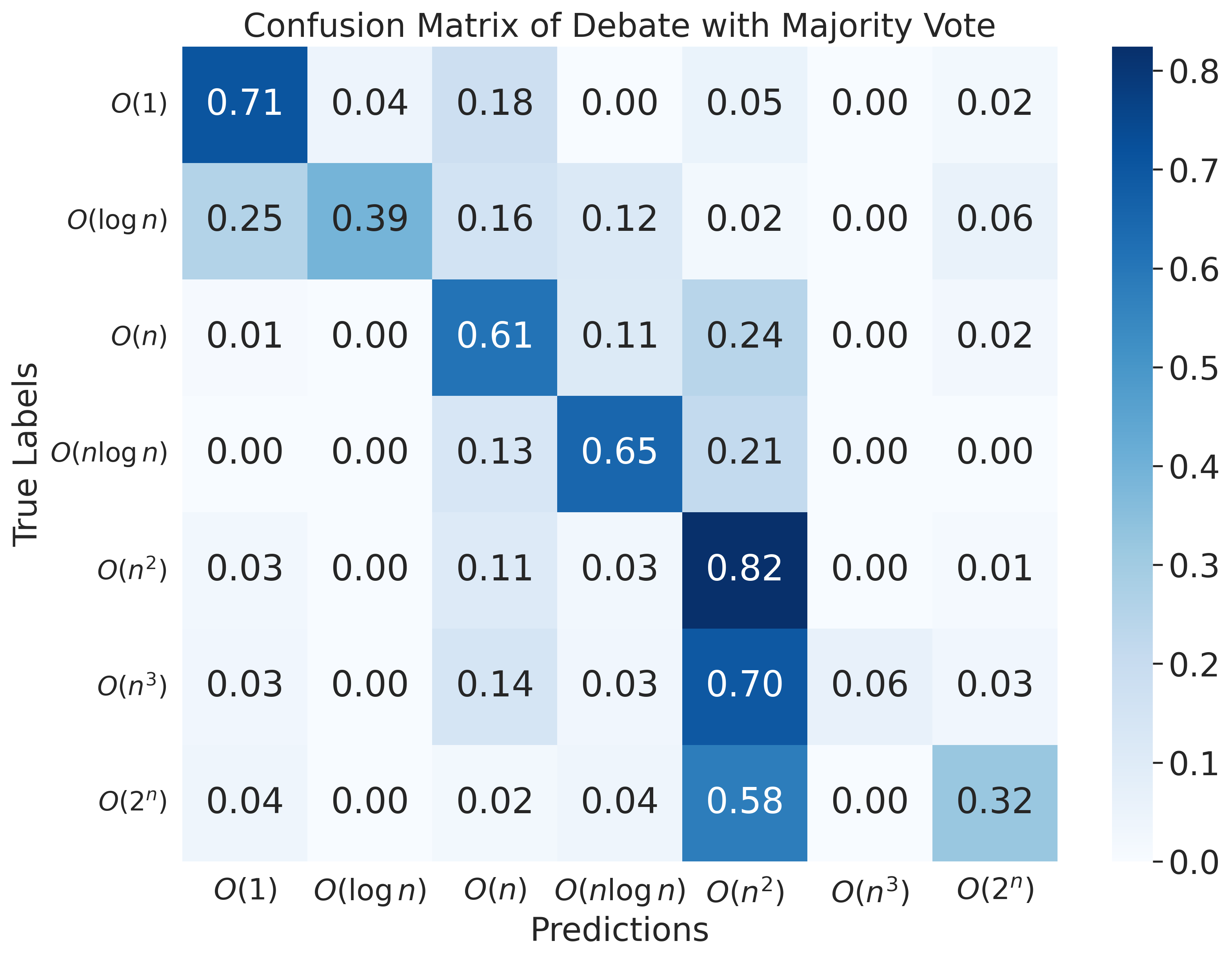
(a) Multiagent (Majority)

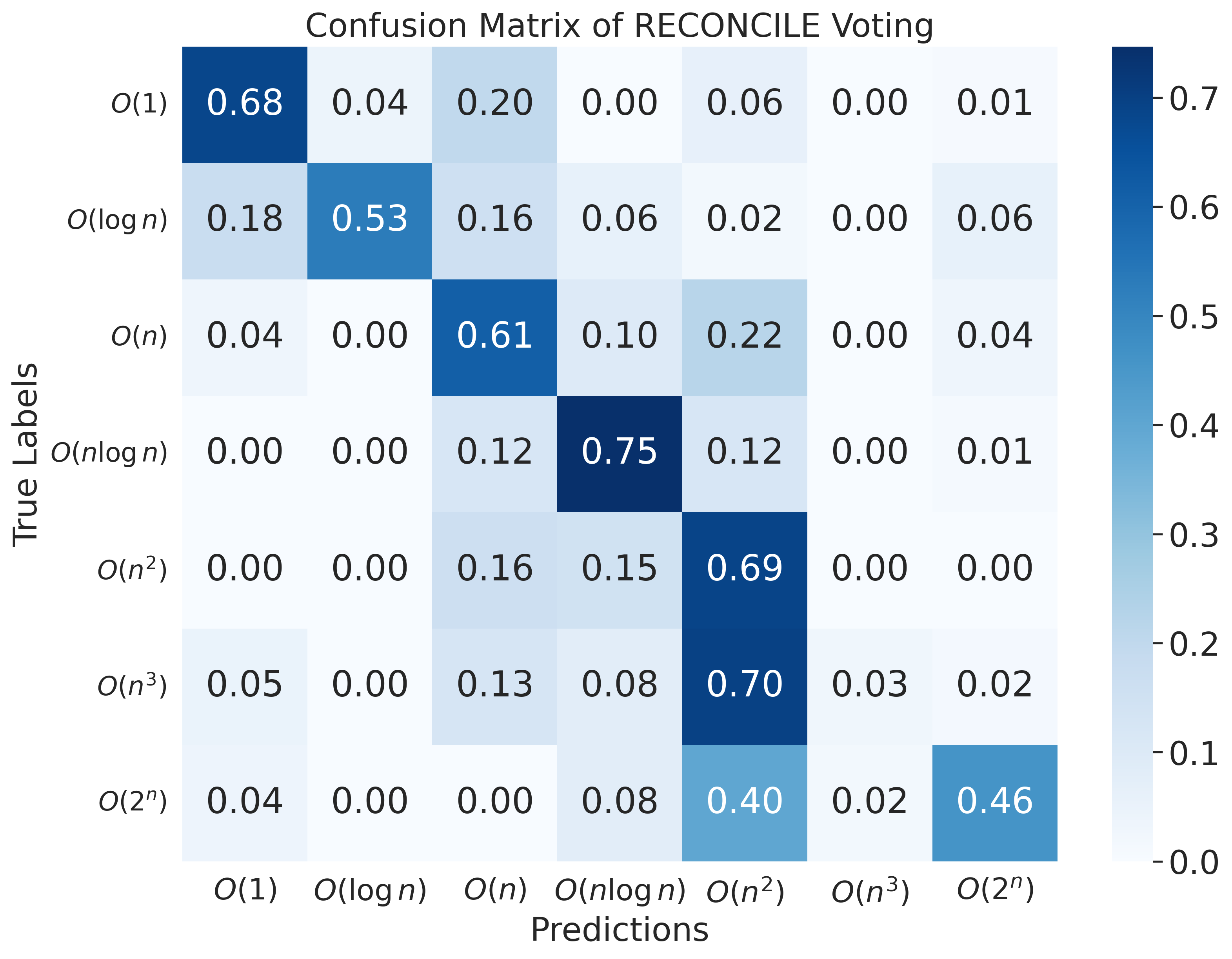
(b) RECONCILE

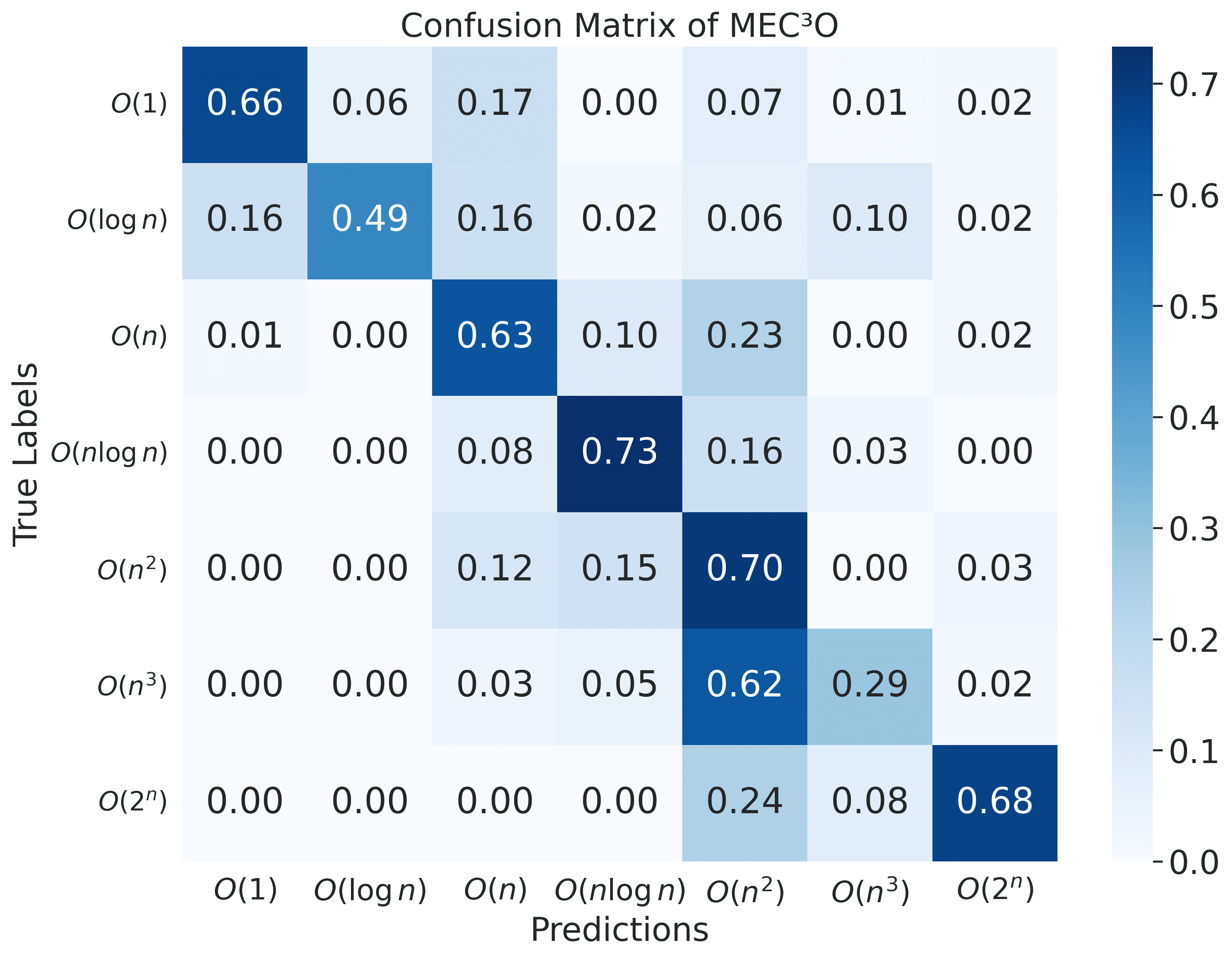
(c) MEC³O

Figure 3: Confusion matrices of Java performance.

Furthermore, we compare the experts who preserve their outputs and those who update their outputs when their predictions match their expertise class. Both cases demonstrate similar performance, but preserving the outputs gives a 4.24% higher F1 score for Java. This observation implies that experts tend to give more accurate predictions that they are specialized to, where the opinions of others might provide potential noise. For instance, when the constant specialist gives outputs of constant predictions, preserving its outputs give better performance of MEC³O.

5.4 Error Analysis

We analyze confusion matrices to assess how MEC³O mitigates class-wise ambiguity and improves robustness over conventional multi-agent baselines. For clarity, we focus on two strong baselines—Multiagent (Majority) and RECONCILE—with full results in Appendix G.

Multiagent (Majority), shown in Figure 3(a), exhibits frequent misclassifications of $O(\log n)$ and $O(n\log n)$ to their adjacent classes due to subtle structural differences. MEC³O resolves much of this confusion, improving $O(\log n)$ and $O(n\log n)$ accuracy by over 10%. This reflects the impact of weighted consensus which enforces clearer decision boundaries, especially between neighboring sublinear and linear patterns. While MEC³O shows on-par performance to RECONCILE in $O(1)$, $O(\log n)$, $O(n)$, $O(n\log n)$, and $O(n^{2})$ classes, it achieves significant improvements in $O(n^{3})$ and $O(2^{n})$ classes in Figures 3(b) and 3(c). This indicates that our expert assignment enables better recognition of nesting structures and exponential behaviors, where other systems struggle.

A key strength of MEC³O lies in its smooth and stable performance across all classes. While the baselines show spikes of strength in some classes and sharp drops in others, MEC³O achieves relatively more stable performance. Nevertheless, MEC³O does not entirely eliminate all forms of confusion. Some confusion remains between $O(n^{2})$ and $O(n^{3})$, which often differ in the depth of nested loops. LLMs may misinterpret nested loops or their scaling semantics, leading to occasional misclassifications. Similarly, some ambiguity among $O(1)$, $O(\log n)$, and $O(n)$) classes persists. Future work may explore more granular expert prompts for close polynomial orders or structured reasoning augmentation to further improve these borderline cases.

6 Conclusion

We introduce MEC³O, which selects a specialized LLM for each time complexity class using a small expertise dataset, then after turning the models into experts with class-specific instructions, coordinates these experts through a debate and a weighted consensus. Our experiments show that this approach mitigates locked-in errors and confusion among classes, achieving at least 10% higher accuracy and F1 scores, surpassing all open-source baselines. MEC³O also proves highly competitive with commercial LLMs, outperforming GPT-4o-mini in F1 score and achieving competitive performance to GPT-4o and GPT-o4-mini on average. These results highlight the value of specialized instructions for code time complexity, the value of multi-expert collaboration, as well as the weighted consensus function that substitutes a judge model.

Limitations

Computational Cost.

MEC³O requires multiple LLMs to process a single input, making it more expensive than single-LLM approaches. However, we avoid the additional cost of a separate judge model, and the system remains feasible with smaller open-source models. Optimizing expert selection or reducing redundant computations could further improve efficiency.

Borderline Class Confusion.

Some complexity classes, such as $O(n^{2})$ and $O(n^{3})$, remain difficult to distinguish, even with expert debate and weighted consensus. MEC³O’s performance on $O(n^{3})$ is comparable to baselines while demonstrating notable advances in other classes. Future improvements could refine how experts interact to handle these edge cases.

Limited Evaluations on Large LLMs.

MEC³O primarily relies on relatively small open-source LLMs with size 7B–8B parameters. This choice is reasonable given the high computational cost of using large proprietary models in a multi-agent setup, but further analysis could investigate whether incorporating larger models as experts would yield additional gains.

Appendix A Expertise Selection

We determine model expertise using a small expertise dataset, which is separate from the test set. Table 4 presents the top-performing LLM for each complexity class across different dataset sampling ratios. Qwen2.5-Coder denotes Qwen2.5-Coder-7B-Instruct, Deepseek-Coder denotes deepseek-coder-7b-instruct-v1.5, Ministral denotes Ministral-8B-Instruct-2410, and Llama-3.1 denotes Meta-Llama-3.1-8B-Instruct in Table 4. Notably, no single LLM excels in all complexity classes. Instead, models from different families demonstrate complementary strengths. For example, Qwen2.5-Coder performs well on logarithmic or linear complexity, whereas Deepseek-Coder and Ministral performs better on linearithmic complexity. Increasing the expertise dataset size (from 10% to 30%) confirms that each model’s expertise remains relatively stable across complexity classes. This consistency allows us to assign models as class-specific experts with high confidence.

Language	First Ranked Model	constant ($O(1)$)	logarithmic ($O(logn)$)	linear ($O(n)$)	linearithmic ($O(nlogn)$)	quadratic ($O(n^{2})$)	cubic ($O(n^{3})$)	exponential ($O(2^{n})$)
Python	10%	Qwen2.5-Coder	Qwen2.5-Coder	Qwen2.5-Coder	Deepseek-Coder	Qwen2.5-Coder	Llama-3.1	Ministral
	20%	Qwen2.5-Coder	Qwen2.5-Coder	Qwen2.5-Coder	Deepseek-Coder	Qwen2.5-Coder	Llama-3.1	Qwen2.5-Coder
	30%	Qwen2.5-Coder	Qwen2.5-Coder	Qwen2.5-Coder	Deepseek-Coder	Qwen2.5-Coder	Llama-3.1	Ministral
Java	10%	Deepseek-Coder	Qwen2.5-Coder	Qwen2.5-Coder	Ministral	Llama-3.1	Llama-3.1	Qwen2.5-Coder
	20%	Ministral	Qwen2.5-Coder	Qwen2.5-Coder	Ministral	Llama-3.1	Deepseek-Coder	Qwen2.5-Coder
	30%	Deepseek-Coder	Qwen2.5-Coder	Qwen2.5-Coder	Ministral	Llama-3.1	Llama-3.1	Qwen2.5-Coder

Table 4: An overview of the first-ranked model for each time complexity. We exploit the model ranks with varying expertise dataset size (10%, 20%, and 30%).

Appendix B Class‐Wise Performance Breakdown for LLMs

We use frequently used open-source LLMs of 7–8B parameter size, as illustrated in Section 4.5. As explained in Section 4.5, for each time complexity class, we select an LLM with the highest performance for the particular class and use the LLM as an expert for that class. Tables 5 and 6 present the performance of each LLM per class. Both tables show that Qwen2.5-Coder, Deepseek-Coder, Ministral, and Llama-3.1 performs the best, each achieving the highest performance for the designated class. Section A presents the model with the top performance per class.

Rate	Model	$O(1)$	$O(\log n)$	$O(n)$	$O(n\log n)$	$O(n^{2})$	$O(n^{3})$	$O(2^{n})$
Java
10%	Qwen2.5-Coder	65.67	47.31	62.03	62.50	50.62	10.53	52.43
	Deepseek-Coder	72.27	33.77	50.00	51.55	39.74	21.62	21.62
	Llama-3.1	46.15	23.68	41.86	46.51	53.62	23.08	19.18
	Ministral	69.63	27.40	53.50	70.37	45.45	0.00	35.29
	Mistral	52.17	37.77	42.64	33.33	32.47	0.00	22.54
	codegemma	9.09	14.49	15.22	11.43	2.99	0.00	0.00
	CodeLlama	31.17	3.08	22.00	21.33	17.46	0.00	0.00
20%	Qwen2.5-Coder	73.61	56.38	53.96	51.00	38.51	2.88	62.56
	Deepseek-Coder	74.56	32.89	38.91	34.94	42.23	22.22	36.27
	Llama-3.1	56.52	34.21	37.36	27.10	44.44	20.65	18.18
	Ministral	74.91	25.00	47.50	52.36	40.82	0.00	41.92
	Mistral	52.46	40.00	40.11	21.43	31.58	1.57	30.26
	codegemma	13.24	9.02	22.46	5.97	1.54	0.00	0.00
	CodeLlama	9.02	7.58	21.28	13.70	18.41	0.00	4.65
30%	Qwen2.5-Coder	70.77	56.34	54.73	55.24	44.31	16.10	58.50
	Deepseek-Coder	70.95	48.84	40.58	52.35	37.95	18.69	6.54
	Llama-3.1	53.79	27.62	36.02	38.71	45.80	19.57	16.35
	Ministral	70.59	27.27	45.49	66.88	42.58	0.00	28.94
	Mistral	51.30	40.49	41.53	19.76	30.98	0.00	25.34
	codegemma	10.05	5.10	16.90	7.69	3.03	1.05	0.00
	CodeLlama	15.61	7.14	21.62	22.73	19.24	2.09	7.14

Table 5: Per‐class accuracy of LLMs on Java subsets by sampling rate.

Rate	Model	$O(1)$	$O(\log n)$	$O(n)$	$O(n\log n)$	$O(n^{2})$	$O(n^{3})$	$O(2^{n})$
Python
10%	Qwen2.5-Coder	64.66	57.43	51.81	39.66	45.51	27.85	15.00
	Deepseek-Coder	60.00	28.57	46.72	51.43	42.77	38.64	17.95
	Llama-3.1	46.81	49.44	37.92	49.12	28.57	40.48	14.08
	Ministral	54.29	22.54	48.35	48.84	36.29	0.00	25.58
	Mistral	47.62	51.69	39.84	5.63	23.20	9.09	0.00
	codegemma	40.96	39.75	36.36	42.55	2.74	6.15	0.00
	CodeLlama	8.70	3.03	7.89	0.00	14.74	9.09	0.00
20%	Qwen2.5-Coder	64.15	55.56	52.38	52.32	42.27	35.37	32.37
	Deepseek-Coder	63.07	33.12	50.68	54.45	41.38	35.44	24.72
	Llama-3.1	42.78	32.68	36.84	29.38	34.55	40.48	8.82
	Ministral	60.87	22.38	47.70	32.91	40.34	0.00	28.92
	Mistral	46.33	35.84	38.39	5.59	24.69	7.63	0.00
	codegemma	35.37	28.95	33.76	40.86	7.19	11.94	0.00
	CodeLlama	11.68	13.24	14.53	10.07	12.50	6.06	0.00
30%	Qwen2.5-Coder	63.75	53.79	49.66	52.12	44.86	29.75	29.23
	Deepseek-Coder	63.25	34.04	45.48	55.75	43.24	35.74	27.07
	Llama-3.1	42.14	36.21	34.11	27.24	28.39	42.02	9.76
	Ministral	61.29	26.48	44.36	31.03	38.04	0.00	29.92
	Mistral	42.91	37.98	38.11	3.77	24.10	7.14	4.08
	codegemma	36.95	26.55	34.38	41.16	4.85	12.87	0.00
	CodeLlama	8.91	10.95	13.14	10.68	11.84	8.04	0.00

Table 6: Per‐class accuracy of LLMs on Python subsets by sampling rate.

Appendix C Single LLM Performance

The single LLM category compares four open-source models under zero- and 7-shot conditions. In the zero-shot setting, a brief instruction about code time complexity prediction is provided without labeled examples; in the 7-shot setup, each model sees seven demonstrations, one per class, along with their assigned time complexities. A key observation is that single LLMs often lock into incorrect reasoning when encountering less familiar code structures.

		Java		Python		Average
	Demonstrations	Acc.	F1.	Acc.	F1.	Acc.	F1.
Qwen2.5-Coder	✗	52.00	44.00	50.20	40.60	51.10	42.30
	✓	56.30	48.90	48.00	39.40	52.15	44.15
deepseek-Coder	✗	36.90	33.40	43.30	39.50	40.10	36.45
	✓	43.90	40.70	40.60	36.70	42.25	38.70
Llama-3.1	✗	32.20	26.70	34.70	27.50	33.45	27.10
	✓	37.80	33.40	34.30	25.90	36.05	29.65
Ministral	✗	44.90	34.30	42.40	30.80	43.65	32.55
	✓	46.90	37.80	43.10	35.80	45.00	36.80
Mistral	✗	33.88	26.52	31.84	21.95	32.86	24.24
	✓	40.00	35.29	33.67	27.24	36.84	31.27
codegemma	✗	25.42	24.02	23.67	23.10	24.55	23.56
	✓	26.12	24.49	29.80	24.28	27.96	24.39
CodeLlama	✗	8.78	10.22	6.94	8.25	7.86	9.24
	✓	4.65	3.92	17.14	17.56	10.90	10.74

Table 7: Accuracy and F1 performance of the baselines. Baselines include seven open-source LLMs. We use zero-shot (✗) and seven-shot (✓) settings.

Appendix D Computational Cost

We measured inference cost in terms of generated tokens. As shown in Table 8, CoT, Self-Consistency, and Reflexion–all single-LLM methods–generate substantially fewer tokens than the multi-agent debate framework. Within MAD, two agents engage in a debate, but the judge often makes an early decision to either conclude or continue, which limits the total token count. MAD generates relatively few tokens compared to other multi-agent approaches, yet it exhibits the lowest performance. MEC³O, by contrast, generates far fewer tokens than CMD and only marginally more than RECONCILE, yet delivers performance gains of 19.12% and 9.38 % in average macro-F1 improvements over these methods. Thus, MEC³O achieves a clear balance of superior effectiveness and efficiency.

Method	Cost (# Generated Tokens)
CoT	239,452
Self-Consistency	897,558
Reflexion	551,253
RECONCILE	2,012,499
CMD	3,219,188
MAD	502,751
MEC3O	2,300,898

Table 8: Total number of tokens processed by each method during inference.

Appendix E Weighted Scores

We evaluate MEC³O and baseline models–including (1) single LLMs and (2) multi-agent approaches–using accuracy and macro F1 in addition to weighted F1. Unlike macro F1, which treats all classes equally, weighted F1 adjusts for class distributions by assigning different weights based on class frequency. This provides a more representative evaluation of model performance across the dataset.

Table 9 presents the full comparison, including weighted F1. Notably, the weighted F1-scores are higher than the macro F1-scores. This is primarily because classes with fewer examples, such as cubic complexity ($O(n^{3})$), contribute less to the overall score compared to more frequent classes.

MEC³O achieves the highest weighted F1 across both Java and Python among open-source baselines, validating its effectiveness in handling diverse complexity classes while maintaining balanced performance. Furthermore, it demonstrates competitive performance to GPT-4o, GPT-4o-mini, and GPT-o4-mini.

	Java			Python			Average
	Acc.	F1.	Weighted F1.	Acc.	F1.	Weighted F1.	Acc.	F1.	Weighted F1
Single LLM
zero-shot Instruction (Brown et al., 2020)	52.00	44.00	51.80	50.20	40.60	49.70	51.10	42.30	50.75
seven-shot Instruction (Brown et al., 2020)	56.30	48.90	56.60	48.00	39.40	47.20	52.15	44.15	51.90
CoT (Wei et al., 2022)	54.08	45.79	53.62	52.86	44.06	52.99	53.47	44.93	53.31
Self-Consistency (Wang et al., 2023)	51.84	42.45	50.28	51.22	40.73	49.69	51.53	41.59	49.99
Reflexion (Shinn et al., 2023)	53.47	43.89	51.70	52.24	41.96	51.38	52.86	42.93	51.54
Multi-Agent Debate
Multiagent (Majority) (Du et al., 2024)	54.49	50.21	52.42	52.86	49.97	51.76	53.68	50.09	52.09
Multiagent (Judge) (Du et al., 2024)	54.90	45.10	53.70	55.30	44.60	54.40	55.10	44.85	54.05
MAD (Liang et al., 2024)	46.33	39.72	46.51	40.00	36.36	43.77	43.17	38.04	45.14
RECONCILE (Chen et al., 2024)	55.92	52.79	53.95	55.31	51.11	54.33	55.62	51.95	54.14
CMD (Wang et al., 2024a)	56.53	47.07	55.61	55.31	45.69	55.02	55.92	46.38	55.32
Commercial LLMs
GPT-4o	71.72	62.22	–	61.09	53.08	–	66.41	57.65	–
GPT-4o-mini	64.96	55.68	–	56.09	48.40	–	60.53	52.04	–
GPT-o4-mini	65.12	62.31	–	62.31	54.23	–	63.72	58.27	–
Multi-Expert with Weighted Consensus
MEC3O	61.02	61.16	61.65	57.55	53.51	56.30	59.29	57.34	58.98

Table 9: Accuracy, F1, and weighted F1 performance of MEC³O and baselines.

Appendix F Statistical Significance of MEC³O

We evaluate whether MEC³O’s performance improvements over baselines in Table 9 are statistically significant by using a paired sign test (Demšar, 2006), a non-parametric test suitable for single-run evaluations. We compare MEC³O to each baseline across six evaluation settings: Accuracy, macro-F1, and weighted-F1 for both Java and Python.

For each baseline, we count the number of settings where MEC³O outperforms it. Under the null hypothesis that both methods are equally good, the probability of a win on any task is 0.5. The one-sided $p$-value is calculated as:

$$p=\sum_{i=k}^{n}\binom{n}{i}\cdot 0.5^{n}$$

where $n=6$ and $k$ is the number of wins. As shown in Table 10, MEC³O achieves perfect wins against every baseline across all six settings.

Baseline	Wins ($k$)	Losses	$p$-value
Zero-Shot Instruction	6	0	0.016*
Seven-Shot Instruction	6	0	0.016*
CoT	6	0	0.016*
Self-Consistency	6	0	0.016*
Reflexion	6	0	0.016*
Multiagent (Majority)	6	0	0.016*
Multiagent (Judge)	6	0	0.016*
MAD	6	0	0.016*
RECONCILE	6	0	0.016*
CMD	6	0	0.016*

Table 10: Paired sign test comparing MEC³O to each baseline across six task-metric pairs. * denotes statistical significance at $\alpha=0.05$.

MEC³O consistently outperforms all baselines across all six metrics, achieving perfect wins in every comparison ($p=0.016$). This significantly rejects the null hypothesis at the 5% level. These results support the claim that MEC³O offers consistent and statistically meaningful gains in accuracy, macro, and weighted F1 scores across languages.

Appendix G Baselines

1. Chain of Thought (CoT) Wei et al. (2022): A brief instruction about code time complexity prediction is provided without labeled examples, and the model is encouraged to generate intermediate reasoning steps to reach a final answer.

2. Self-Consistency Wang et al. (2023): It extends CoT by sampling multiple reasoning paths and selecting the most consistent answer through majority voting.

3. Reflexion Shinn et al. (2023): Reflexion enables agents to improve through verbal self-reflection rather than weight updates. After each trial, agents generate natural language feedback based on outcomes and store it in memory to guide future decisions.

4. Multiagent Du et al. (2024): Each agent first generates its own response independently. Then, during the debate phase, agents exchange and reason over the responses of others, excluding their own. The final answer is determined via a majority vote or a separate judge model.

5. MAD Liang et al. (2024): The proposed framework consists of two agents–an affirmative and a negative one–who engage in a debate. The affirmative agent first generates a response, after which the negative agent produces a counter-argument. A separate judge model then decides whether to proceed with additional debate rounds or to conclude with a final decision based on the current arguments.

6. RECONCILE Chen et al. (2024): Each agent generates an answer with a confidence score. After several rounds of discussion, a final answer is selected via confidence-weighted voting, where each agent’s vote is weighted by its calibrated confidence.

7. CMD Wang et al. (2024a): Agents are divided into two groups. While agents within the same group share both answers and explanations, only answers are exchanged across groups. A majority vote determines the final answer, with a secretary agent resolving ties if necessary.

G.1 CoT Analysis

CoT prompting guides the model to lay out its intermediate reasoning steps before arriving at a final answer. By making its “thinking” explicit, CoT can uncover hidden reasoning patterns that lead to correct solutions. However, CoT is susceptible to DoT. Once the model commits to an initial reasoning trajectory, it rarely backtracks to correct flawed premises, causing early mistakes to propagate all the way through the final judgment.

The confusion matrices in Figure 4 provide further insight into this behavior. For both Java and Python, CoT demonstrates strong accuracy on simpler classes such as $O(1)$ and $O(n)$, and particularly excels on $O(n^{2})$ in the Java setting with an accuracy of 70%. However, the model consistently struggles with higher complexity classes like $O(n^{3})$ and $O(2^{n})$, which are frequently misclassified into adjacent lower-complexity classes–for instance, $O(n^{3})$ is often predicted as $O(n^{2})$. These errors reveal a tendency to default to more familiar or simpler reasoning patterns when the structural signals are ambiguous or sparse. This supports the interpretation that CoT’s explicit reasoning process, while beneficial for transparency, can also lead to rigid thinking paths that reinforce early misconceptions rather than revise them–underscoring its vulnerability to DoT.

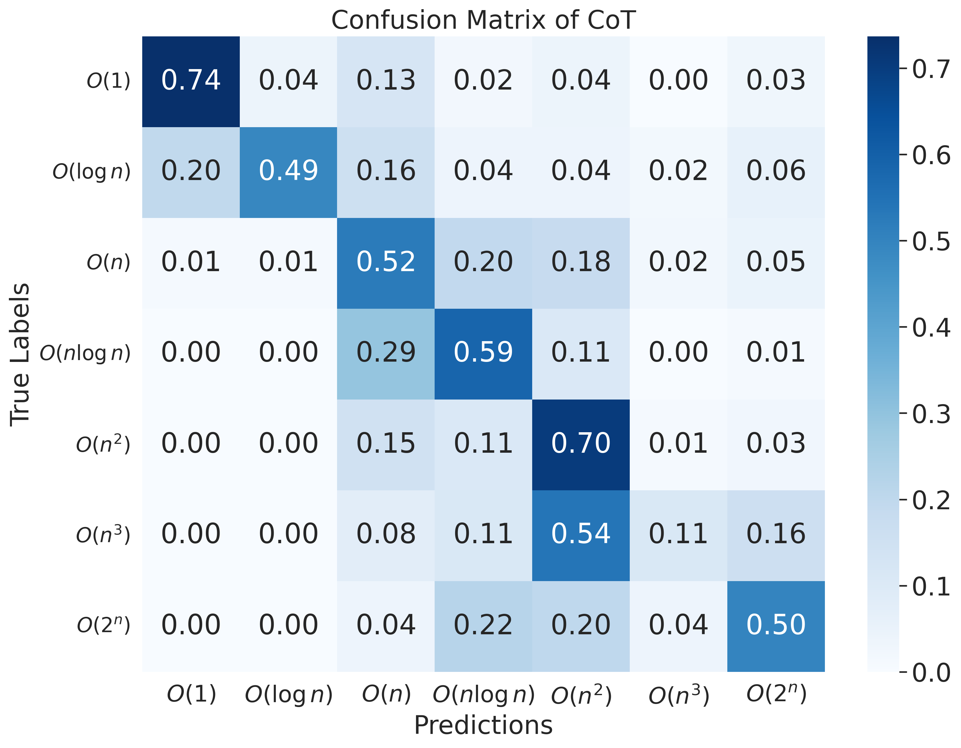
(a) Java

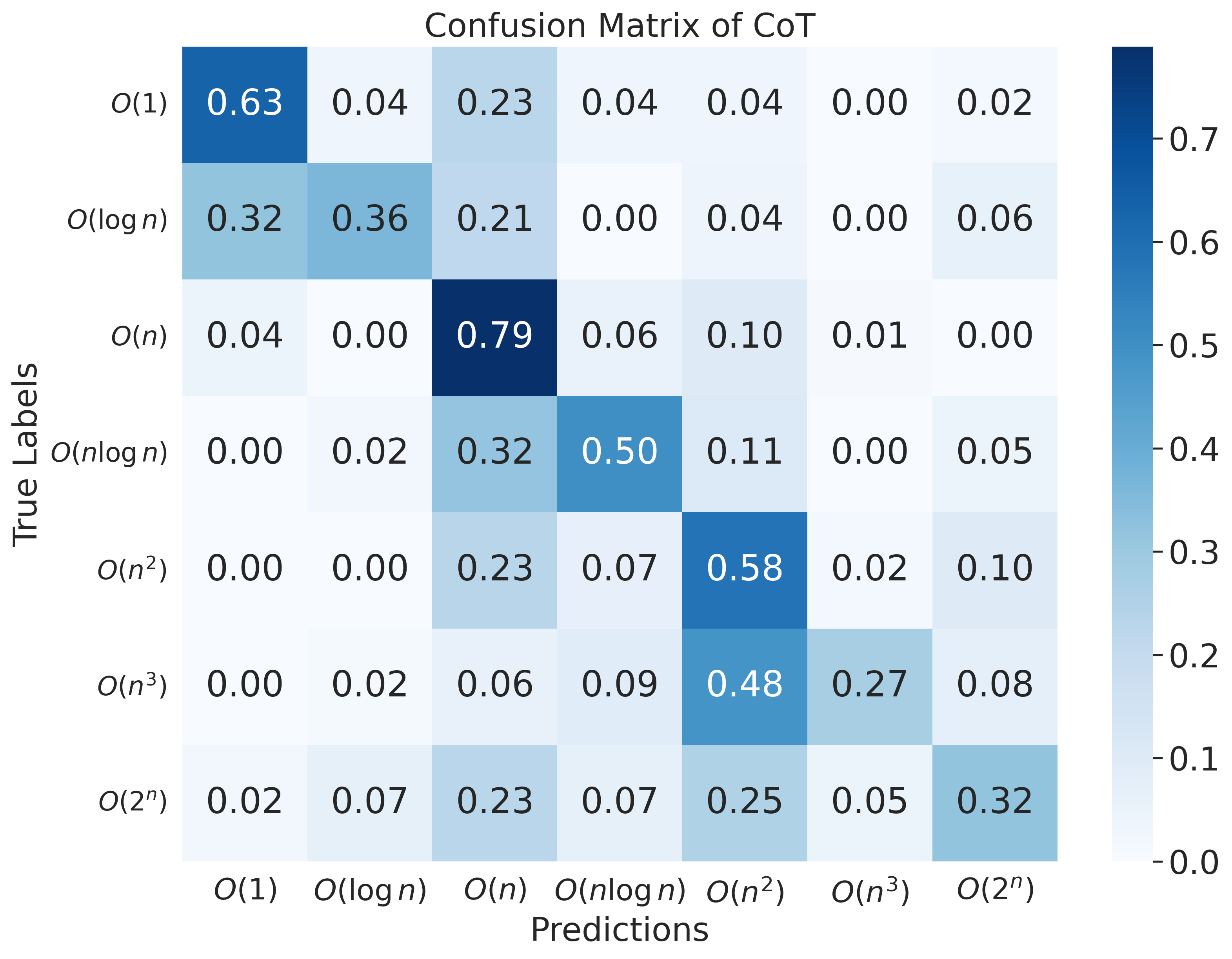
(b) Python

Figure 4: CoT confusion matrices for Java and Python.

G.2 Self-Consistency Analysis

Self-Consistency reduces output variability by sampling several independent reasoning paths and choosing the most frequent answer. This voting approach curbs random fluctuations, but reinforces the model’s built-in reasoning biases. As a result, performance gains tend to be confined to problem types that already match those biases, rather than fostering truly robust reasoning across diverse cases.

The confusion matrices in Figure 5 provide further evidence of this bias reinforcement. While Self-Consistency improves performance for frequently occurring and structurally simple classes such as $O(1)$ and $O(n)$, it performs notably worse on higher complexity classes like $O(n^{3})$ and $O(2^{n})$. In both Java and Python, these classes are frequently misclassified into simpler categories, indicating that the majority-vote mechanism amplifies the model’s tendency to converge on safe, low-complexity predictions. As a result, Self-Consistency may stabilize outputs but fails to recover from biased reasoning paths, particularly when confronting edge-case or rare complexity patterns.

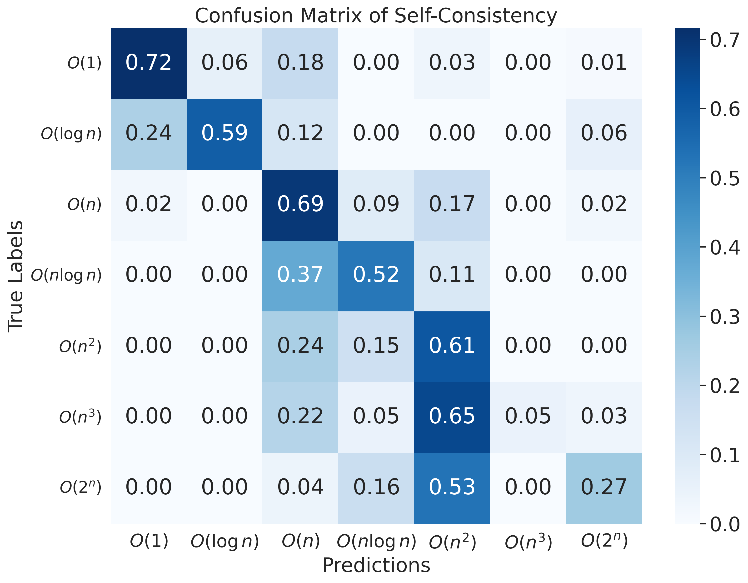
(a) Java

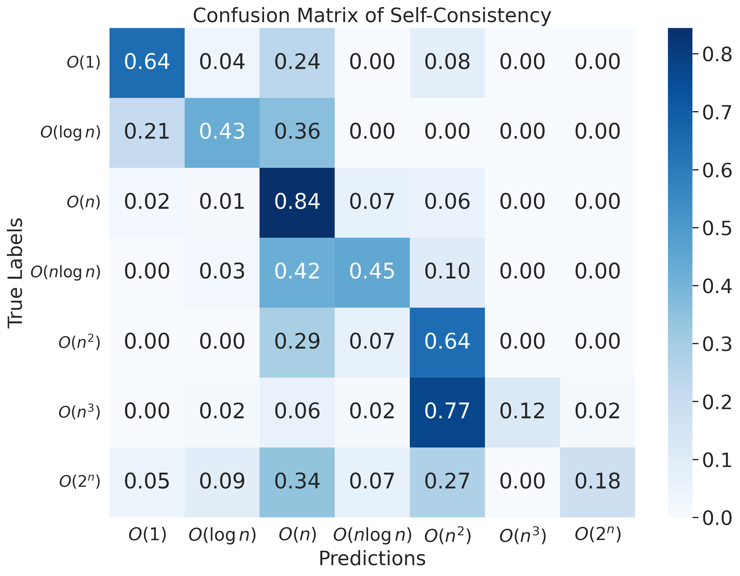
(b) Python

Figure 5: Self-Consistency confusion matrices for Java and Python.

G.3 Reflexion Analysis

Reflexion extends CoT paradigm by introducing a self-reflection loop. After generating an initial inference, the model produces a natural language summary of its own performance and stores it in memory. These stored reflections serve as semantic signals to guide subsequent attempts. However, the loop can become fixed to the initial inference, meaning that early errors persist. When feedback originates from similarly biased reasoning or lacks sufficient corrective cues, the model fails to overcome those errors, leading to a failure mode known as DoT.

Figure 6 shows that Reflexion offers marginal improvements in certain complexity classes, such as $O(n^{2})$ and $O(n^{3})$, particularly in the Python setting. However, its performance remains inconsistent across the full range of complexity levels. For instance, in the Java confusion matrix, Reflexion achieves moderate accuracy on $O(2^{n})$, but still exhibits substantial confusion with neighboring polynomial classes. Notably, predictions for $O(n^{3})$ and $O(2^{n})$ often spill into $O(n^{2})$, indicating that the model’s reflective revisions do not reliably correct initial biases. Instead, reflection tends to reinforce early reasoning paths unless strong corrective signals are available. This observation supports the concern that, despite offering semantically richer feedback than CoT, Reflexion may still perpetuate flawed inferences when the internal reflections are themselves biased or uninformative.

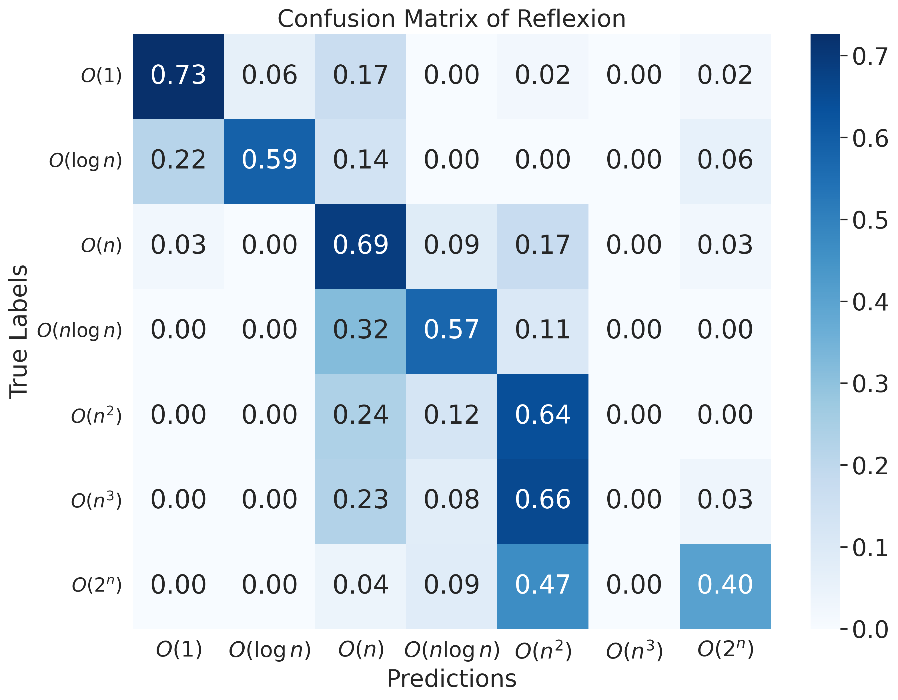
(a) Java

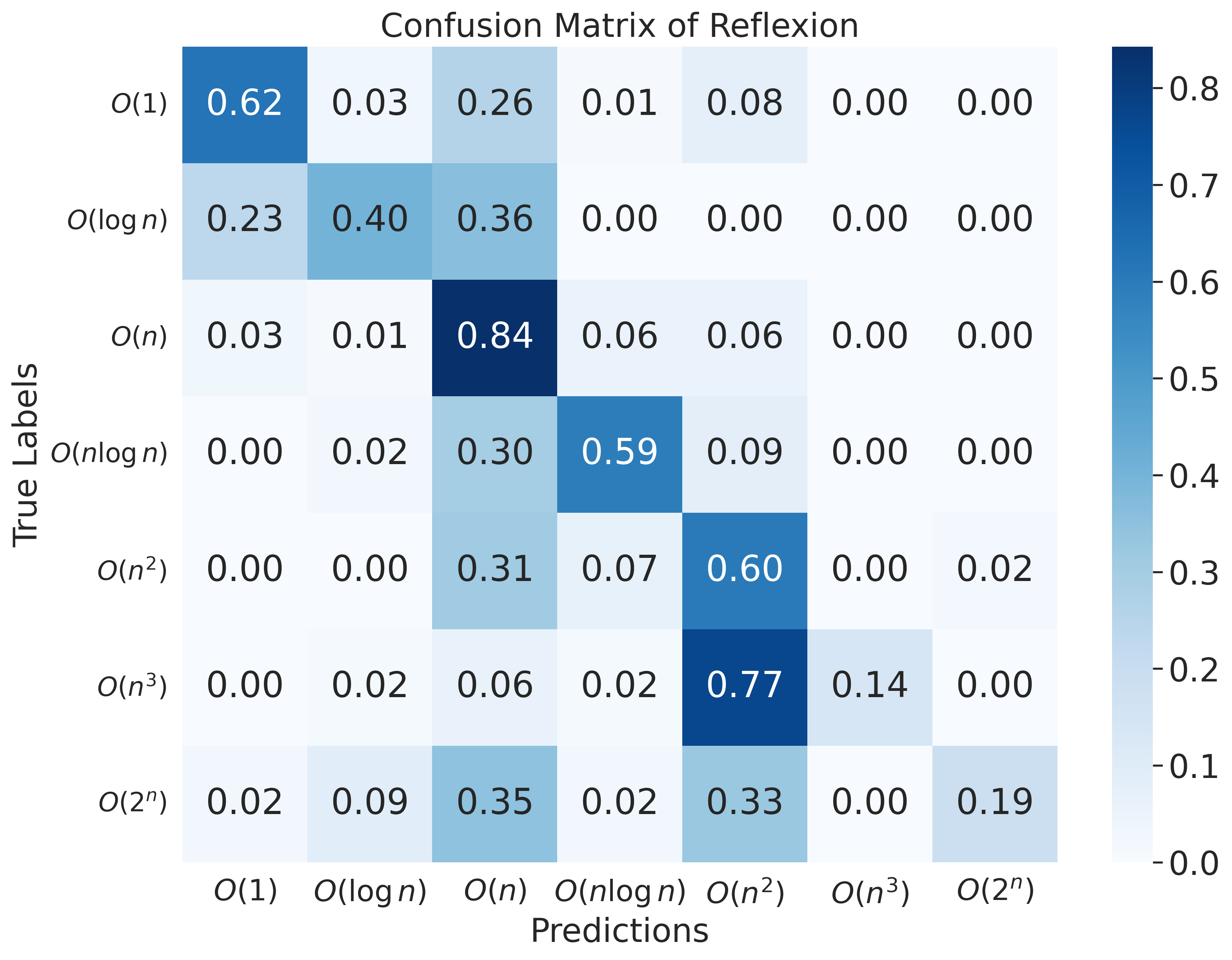
(b) Python

Figure 6: Reflexion confusion matrices for Java and Python.

G.4 Multiagent Analysis

Multiagent (Majority) relies on conventional majority voting to finalize predictions. While this approach enables simple collaborative reasoning, it does not leverage the specific expertise of each model’s class. Consequently, incorrect majority opinions get amplified, and correct answers proposed by minority agents are often ignored, limiting overall reliability.

Figure 7 demonstrates that majority voting stabilizes predictions for certain mid-range complexity classes, most notably $O(n^{2})$. However, its effectiveness diminishes for higher complexity classes. In particular, $O(n^{3})$ and $O(2^{n})$ is frequently misclassified as $O(n^{2})$. This suggests that majority-based reasoning tends to converge on dominant but suboptimal answers, amplifying collective biases rather than correcting them. Consequently, the approach fails to capture correct minority insights, especially when distinguishing between adjacent high-complexity classes.

(a) Java

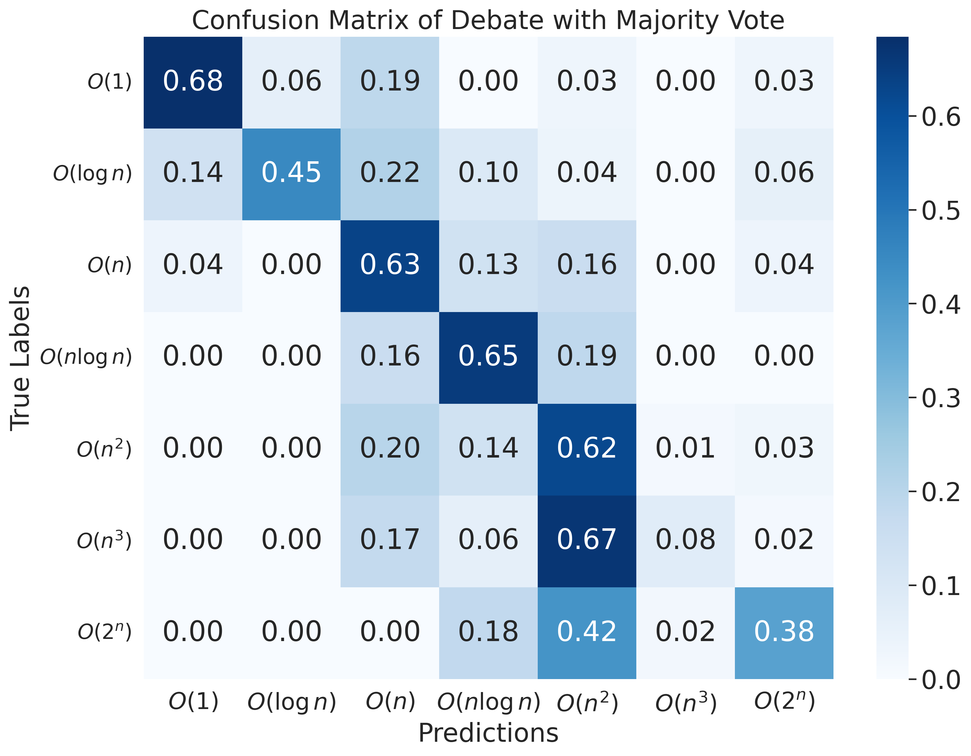
(b) Python

Figure 7: Multiagent (Majority) confusion matrices for Java and Python.

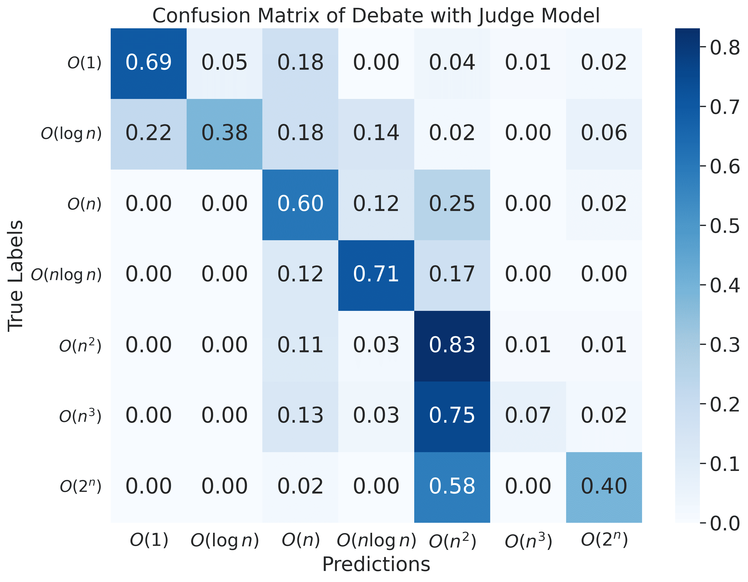
(a) Java

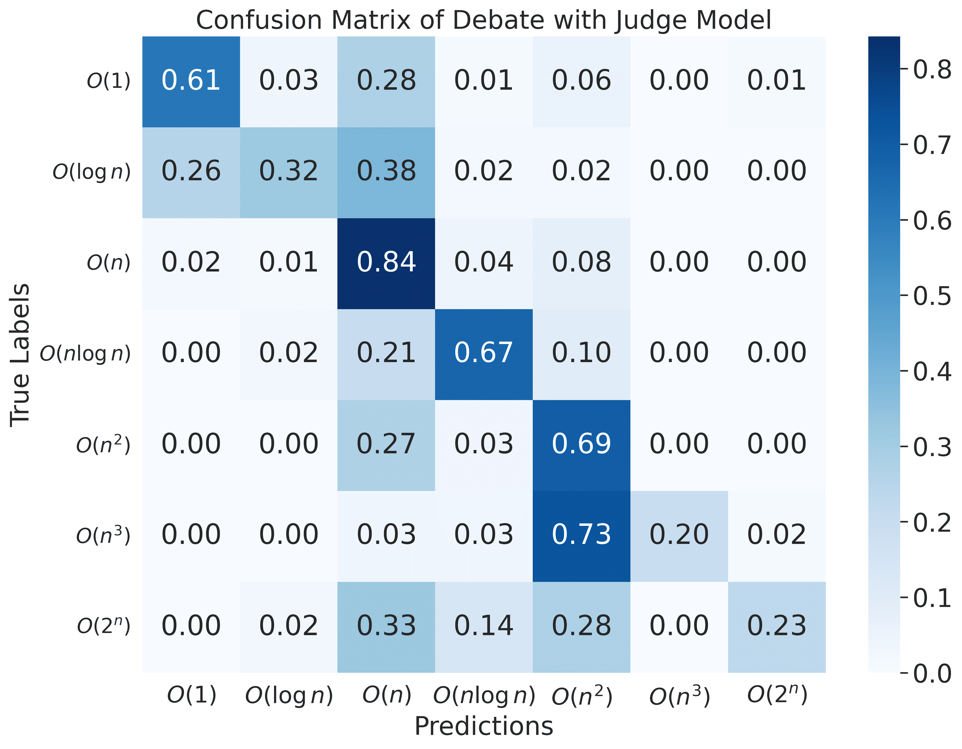
(b) Python

Figure 8: Multiagent (Judge) confusion matrices for Java and Python.

Multiagent (Judge) allocates the final decision to a separate judge model. This can help resolve ties or ambiguous votes, but it still fails to fully leverage individual agents’ strengths. The judge may unduly favor patterns seen during its own training, amplifying certain biases and overlooking minority-supported correct answers, which also constrains reliability.

Figure 8 shows that while the judge model improves prediction consistency for some mid-range classes, it fails to yield performance gains over the majority vote approach presented in Figure 7. In particular, predictions for $O(n^{3})$ remain inaccurate, with many examples misclassified as $O(n^{2})$. This pattern suggests that the judge model does not provide effective correction beyond the aggregation strategy used in majority voting.

G.5 MAD Analysis

In the MAD framework, even when the affirmative agent generates a correct response, the subsequent counterargument provided by the negative agent can degrade the overall performance. Our analysis reveals that the affirmative agent outperforms the negative agent in specific complexity classes such as $O(\log n)$ and $O(n)$. However, in these cases, the negative agent often fails to offer meaningful rebuttals, leading to a significant drop in overall accuracy. Since the final decision is made by a judge model that selects one of the two agents’ outputs, the individual strengths of each agent are not fully reflected in the final outcome. This reliance on a single judge can result in suboptimal decisions, especially when one agent consistently demonstrates superior performance on particular types of problems.

Figure 9 highlights the limitations of the MAD framework in lower-complexity classes. While performance on $O(n\log n)$ and $O(n^{2})$ remains strong, the model shows poor accuracy on $O(\log n)$ and $O(n)$ in both Java and Python. These trends suggest that the back-and-forth debate may not always converge toward the correct solution, particularly when the final judgment relies on binary selection. Compared to other approaches such as majority vote or judge-based models, MAD underperforms in simpler cases that require fine-grained loop analysis.

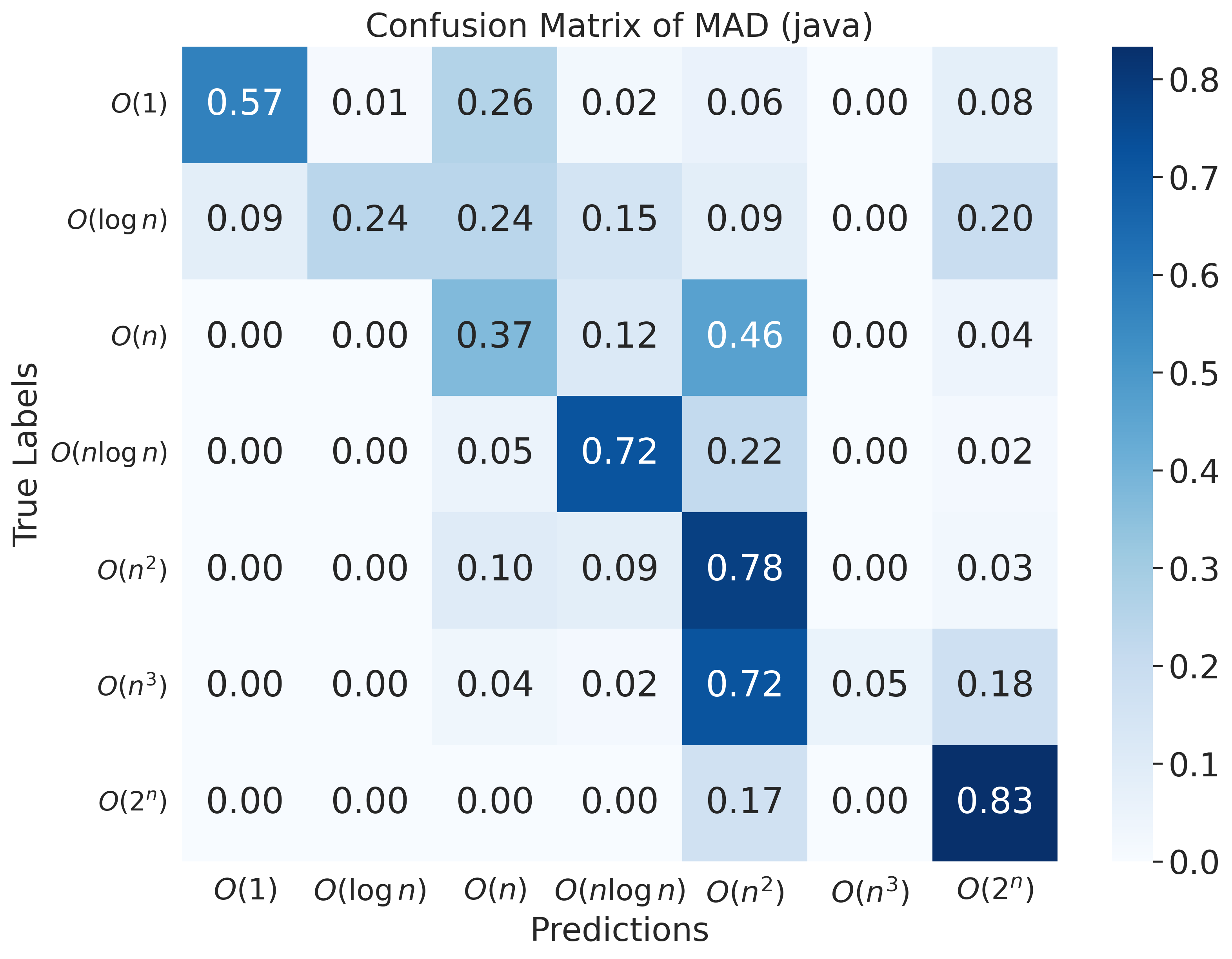
(a) Java

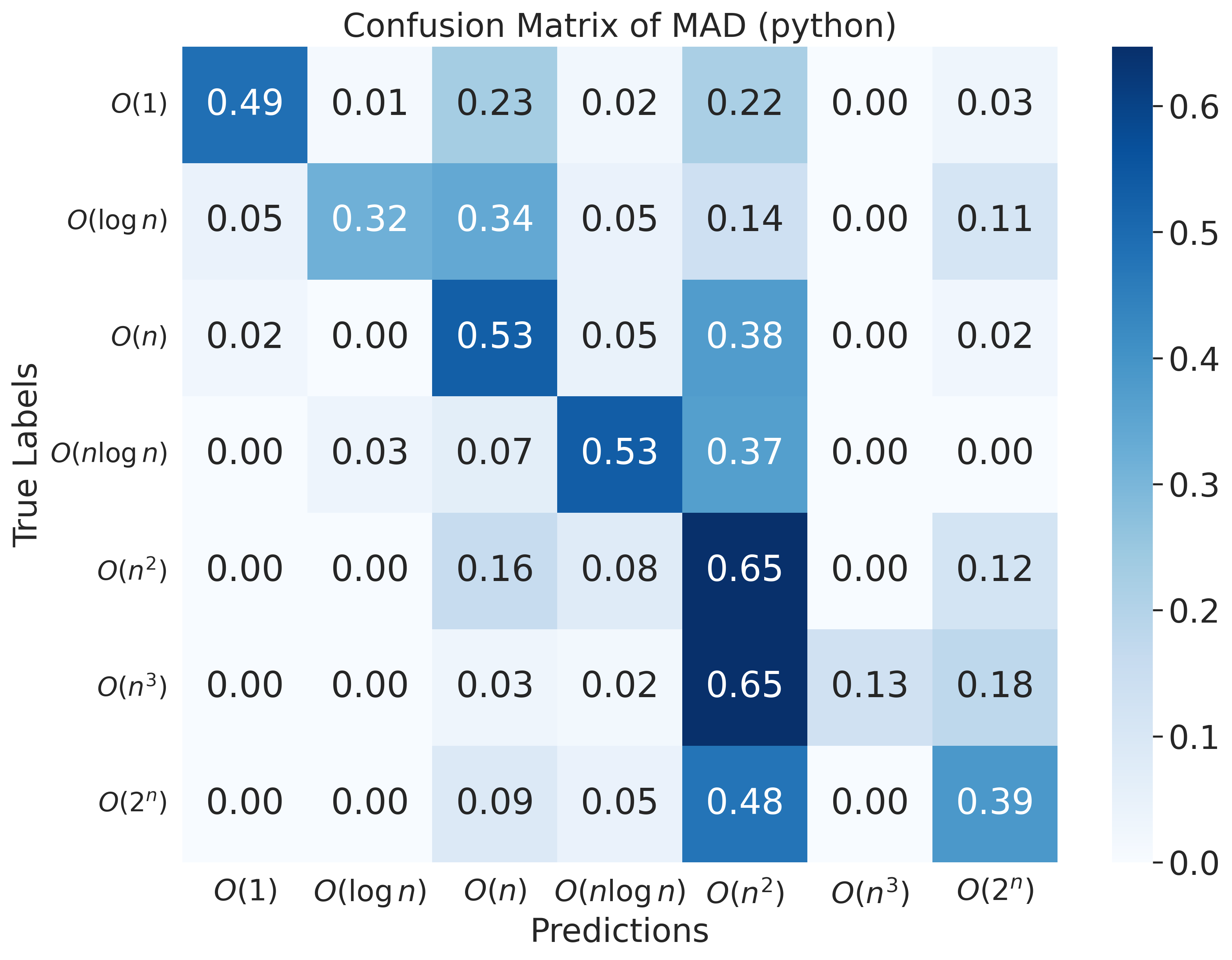
(b) Python

Figure 9: MAD confusion matrices for Java and Python.

G.6 RECONCILE Analysis

RECONCILE determines the final answer using confidence-weighted voting, where each agent’s vote is weighted by its estimated confidence. However, since the answer with the highest total confidence is selected, correct minority opinions can be overshadowed by incorrect majority responses with higher cumulative confidence. As a result, even when some agents provide the correct answer, it can be ignored if most agents confidently support an incorrect one, leading to degraded performance. Nevertheless, the use of confidence scores still provides a meaningful signal, suggesting that model-level uncertainty estimation can effectively guide collaborative reasoning.

Figure 10 confirms that RECONCILE achieves reliable performance on mid-complexity classes such as $O(n\log n)$, demonstrating consistent accuracy across both Java and Python. However, it underperforms on higher-complexity classes like $O(n^{3})$ and $O(2^{n})$, with frequent misclassifications into lower-complexity neighbors. This pattern suggests that confidence-weighted voting can amplify overconfident yet incorrect majority views, particularly when miscalibrated agents dominate the final outcome.

(a) Java

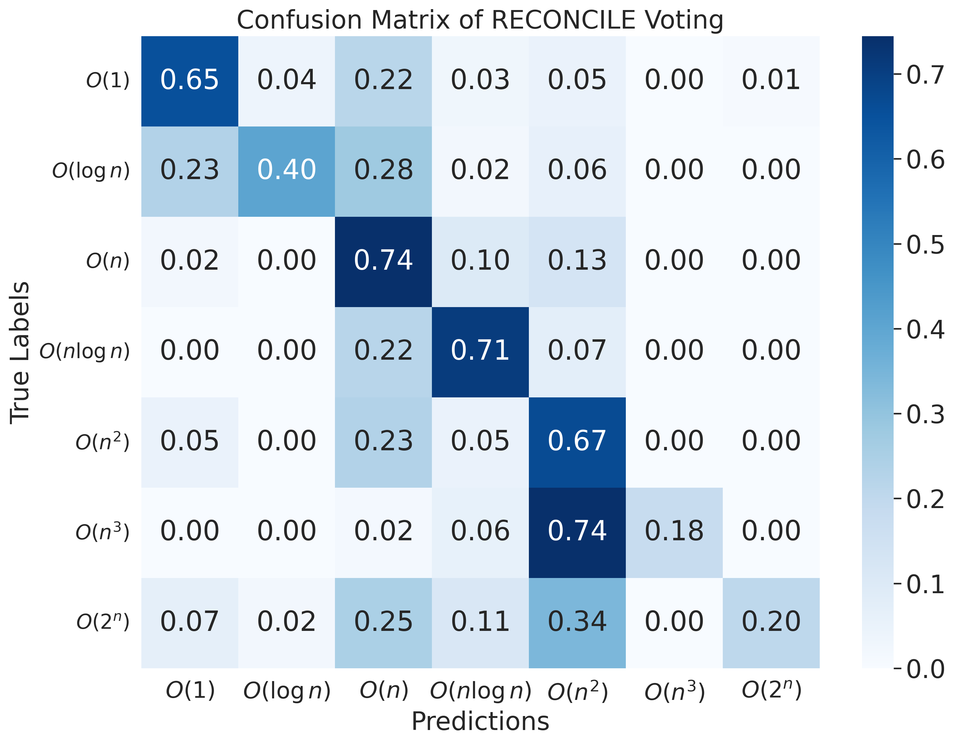
(b) Python

Figure 10: RECONCILE confusion matrices for Java and Python.

Appendix H Instruction for Constant-Time Complexity Expert

Appendix I Instruction for Logarithmic-Time Complexity Expert

Appendix J Instruction for Linear-Time Complexity Expert

Appendix K Instruction for Linearithmic-Time Complexity Expert

Appendix L Instruction for Quadratic-Time Complexity Expert

Appendix M Instruction for Cubic-Time Complexity Expert

Appendix N Instruction for Exponential-Time Complexity Expert

Appendix O Debate Workflow of MEC³O

Figure 11 illustrates how a designated expert in the MEC³O framework initially produces a prediction independently, and subsequently revises the output after considering the opinions of other experts.

The top section (“Initial Output”) shows the response generated by a constant-time complexity expert based solely on class-specific instructions. At this stage, the expert acts independently, without access to peer feedback.

In the middle section (“Debate-Based Instruction”), the expert is exposed to predictions and rationale provided by other models, each specializing in different complexity classes. These external insights allow the expert to identify overlooked patterns or reassess assumptions about the code’s structure–particularly loops or recursive calls that may not have been detected initially.

The bottom section (“Updated Output”) presents the final response after incorporating the opinions of multiple experts. This process is deliberately designed to allow each expert to preserve its strengths in its designated complexity class, while also remaining receptive to critiques from others. As a result, the system promotes more accurate and convincing time complexity predictions.

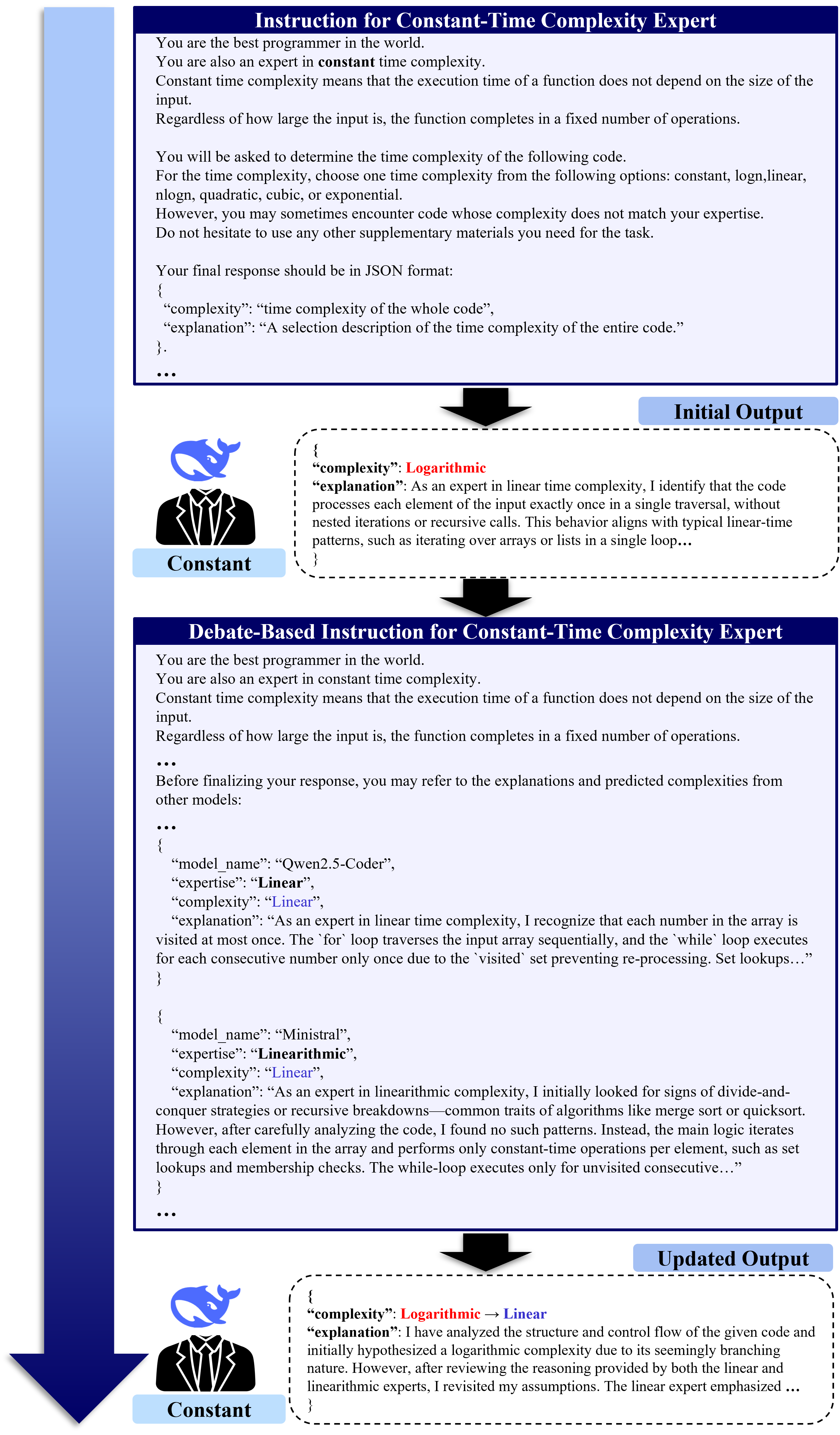
Figure 11: The procedure of debate in MEC³O.

References

- Ahmed et al. (2024) Toufique Ahmed, Kunal Suresh Pai, Premkumar T. Devanbu, and Earl T. Barr. 2024. Automatic semantic augmentation of language model prompts (for code summarization). In Proceedings of the 46th IEEE/ACM International Conference on Software Engineering, ICSE, pages 220:1–220:13.
- Aycock and Bawden (2024) Seth Aycock and Rachel Bawden. 2024. Topic-guided example selection for domain adaptation in llm-based machine translation. In Proceedings of the 18th Conference of the European Chapter of the Association for Computational Linguistics, EACL: Student Research Workshop, pages 175–195.
- Baik et al. (2025) Seung-Yeop Baik, Joonghyuk Hahn, Jungin Kim, Aditi, Mingi Jeon, Yo-Sub Han, and Sang-Ki Ko. 2025. CodeComplex: Dataset for worst-case time complexity prediction. In Findings of the Association for Computational Linguistics: EMNLP.
- Bouzenia et al. (2024) Islem Bouzenia, Premkumar T. Devanbu, and Michael Pradel. 2024. Repairagent: An autonomous, llm-based agent for program repair. ArXiV Preprint, CoRR 2403.17134.
- Brown et al. (2020) Tom B. Brown, Benjamin Mann, Nick Ryder, Melanie Subbiah, Jared Kaplan, Prafulla Dhariwal, Arvind Neelakantan, Pranav Shyam, Girish Sastry, Amanda Askell, Sandhini Agarwal, Ariel Herbert-Voss, Gretchen Krueger, Tom Henighan, Rewon Child, Aditya Ramesh, Daniel M. Ziegler, Jeffrey Wu, Clemens Winter, and 12 others. 2020. Language models are few-shot learners. In Advances in Neural Information Processing Systems 33: Annual Conference on Neural Information Processing Systems, NeurIPS.
- Chen et al. (2024) Justin Chih-Yao Chen, Swarnadeep Saha, and Mohit Bansal. 2024. Reconcile: Round-table conference improves reasoning via consensus among diverse llms. In Proceedings of the 62nd Annual Meeting of the Association for Computational Linguistics, ACL, pages 7066–7085.
- Coignion et al. (2024) Tristan Coignion, Clément Quinton, and Romain Rouvoy. 2024. A performance study of llm-generated code on leetcode. In Proceedings of the 28th International Conference on Evaluation and Assessment in Software Engineering, EASE, pages 79–89.
- Creswell et al. (2023) Antonia Creswell, Murray Shanahan, and Irina Higgins. 2023. Selection-inference: Exploiting large language models for interpretable logical reasoning. In The Eleventh International Conference on Learning Representations, ICLR.
- Demšar (2006) Janez Demšar. 2006. Statistical comparisons of classifiers over multiple data sets. Journal of Machine Learning Research, 7:1–30.
- Du et al. (2024) Yilun Du, Shuang Li, Antonio Torralba, Joshua B. Tenenbaum, and Igor Mordatch. 2024. Improving factuality and reasoning in language models through multiagent debate. In Forty-first International Conference on Machine Learning, ICML.
- Dubey and et al. (2024) Abhimanyu Dubey and et al. 2024. The llama 3 herd of models. ArXiV Preprint, CoRR 2407.21783.
- Guo et al. (2024) Daya Guo, Qihao Zhu, Dejian Yang, Zhenda Xie, Kai Dong, Wentao Zhang, Guanting Chen, Xiao Bi, Y. Wu, Y. K. Li, Fuli Luo, Yingfei Xiong, and Wenfeng Liang. 2024. Deepseek-coder: When the large language model meets programming - the rise of code intelligence. ArXiV Preprint, CoRR 2401.14196.
- Haldar and Hockenmaier (2024) Rajarshi Haldar and Julia Hockenmaier. 2024. Analyzing the performance of large language models on code summarization. In Proceedings of the 2024 Joint International Conference on Computational Linguistics, Language Resources and Evaluation, LREC/COLING, pages 995–1008.
- Hui et al. (2024) Binyuan Hui, Jian Yang, Zeyu Cui, Jiaxi Yang, Dayiheng Liu, Lei Zhang, Tianyu Liu, Jiajun Zhang, Bowen Yu, Kai Dang, An Yang, Rui Men, Fei Huang, Xingzhang Ren, Xuancheng Ren, Jingren Zhou, and Junyang Lin. 2024. Qwen2.5-coder technical report. ArXiV Preprint, CoRR 2409.12186.
- Jiang et al. (2023) Albert Q. Jiang, Alexandre Sablayrolles, Arthur Mensch, Chris Bamford, Devendra Singh Chaplot, Diego de Las Casas, Florian Bressand, Gianna Lengyel, Guillaume Lample, Lucile Saulnier, Lélio Renard Lavaud, Marie-Anne Lachaux, Pierre Stock, Teven Le Scao, Thibaut Lavril, Thomas Wang, Timothée Lacroix, and William El Sayed. 2023. Mistral 7b. ArXiV Preprint, CoRR 2310.06825.
- Li et al. (2023) Yuang Li, Yu Wu, Jinyu Li, and Shujie Liu. 2023. Prompting large language models for zero-shot domain adaptation in speech recognition. In IEEE Automatic Speech Recognition and Understanding Workshop, ASRU, pages 1–8.
- Liang et al. (2024) Tian Liang, Zhiwei He, Wenxiang Jiao, Xing Wang, Yan Wang, Rui Wang, Yujiu Yang, Shuming Shi, and Zhaopeng Tu. 2024. Encouraging divergent thinking in large language models through multi-agent debate. In Proceedings of the 2024 Conference on Empirical Methods in Natural Language Processing, EMNLP, pages 17889–17904.
- Lu et al. (2021) Shuai Lu, Daya Guo, Shuo Ren, Junjie Huang, Alexey Svyatkovskiy, Ambrosio Blanco, Colin B. Clement, Dawn Drain, Daxin Jiang, Duyu Tang, Ge Li, Lidong Zhou, Linjun Shou, Long Zhou, Michele Tufano, Ming Gong, Ming Zhou, Nan Duan, Neel Sundaresan, and 3 others. 2021. Codexglue: A machine learning benchmark dataset for code understanding and generation. In Proceedings of the Neural Information Processing Systems Track on Datasets and Benchmarks 1, NeurIPS Datasets and Benchmarks.
- Madaan et al. (2023) Aman Madaan, Niket Tandon, Prakhar Gupta, Skyler Hallinan, Luyu Gao, Sarah Wiegreffe, Uri Alon, Nouha Dziri, Shrimai Prabhumoye, Yiming Yang, Shashank Gupta, Bodhisattwa Prasad Majumder, Katherine Hermann, Sean Welleck, Amir Yazdanbakhsh, and Peter Clark. 2023. Self-refine: Iterative refinement with self-feedback. In Advances in Neural Information Processing Systems 36: Annual Conference on Neural Information Processing Systems, NeurIPS.
- Nam et al. (2024) Daye Nam, Andrew Macvean, Vincent J. Hellendoorn, Bogdan Vasilescu, and Brad A. Myers. 2024. Using an LLM to help with code understanding. In Proceedings of the 46th IEEE/ACM International Conference on Software Engineering, ICSE, pages 97:1–97:13.
- OpenAI (2023) OpenAI. 2023. GPT-4 technical report. ArXiV Preprint, CoRR 2303.08774.
- Opitz and Burst (2019) Juri Opitz and Sebastian Burst. 2019. Macro F1 and macro F1. ArXiV Preprint, CoRR 1911.03347.
- Peng et al. (2021) Dinglan Peng, Shuxin Zheng, Yatao Li, Guolin Ke, Di He, and Tie-Yan Liu. 2021. How could neural networks understand programs? In Proceedings of the 38th International Conference on Machine Learning, ICML, volume 139 of Proceedings of Machine Learning Research, pages 8476–8486.
- Rozière et al. (2023) Baptiste Rozière, Jonas Gehring, Fabian Gloeckle, Sten Sootla, Itai Gat, Xiaoqing Ellen Tan, Yossi Adi, Jingyu Liu, Tal Remez, Jérémy Rapin, Artyom Kozhevnikov, Ivan Evtimov, Joanna Bitton, Manish Bhatt, Cristian Canton-Ferrer, Aaron Grattafiori, Wenhan Xiong, Alexandre Défossez, Jade Copet, and 6 others. 2023. Code llama: Open foundation models for code. ArXiV Preprint, CoRR 2308.12950.
- Shinn et al. (2023) Noah Shinn, Federico Cassano, Ashwin Gopinath, Karthik Narasimhan, and Shunyu Yao. 2023. Reflexion: language agents with verbal reinforcement learning. In Advances in Neural Information Processing Systems 36: Annual Conference on Neural Information Processing Systems, NeurIPS.
- Sikka et al. (2020) Jagriti Sikka, Kushal Satya, Yaman Kumar, Shagun Uppal, Rajiv Ratn Shah, and Roger Zimmermann. 2020. Learning based methods for code runtime complexity prediction. In Advances in Information Retrieval - 42nd European Conference on IR Research, ECIR, Proceedings, Part I, volume 12035 of Lecture Notes in Computer Science, pages 313–325.
- Wang et al. (2024a) Qineng Wang, Zihao Wang, Ying Su, Hanghang Tong, and Yangqiu Song. 2024a. Rethinking the bounds of LLM reasoning: Are multi-agent discussions the key? In Proceedings of the 62nd Annual Meeting of the Association for Computational Linguistics, ACL, pages 6106–6131.
- Wang et al. (2024b) Shouda Wang, Weijie Zheng, and Benjamin Doerr. 2024b. Choosing the right algorithm with hints from complexity theory. Information and Computation, 296:105125.
- Wang et al. (2023) Xuezhi Wang, Jason Wei, Dale Schuurmans, Quoc V. Le, Ed H. Chi, Sharan Narang, Aakanksha Chowdhery, and Denny Zhou. 2023. Self-consistency improves chain of thought reasoning in language models. In The Eleventh International Conference on Learning Representations, ICLR.
- Wei et al. (2022) Jason Wei, Xuezhi Wang, Dale Schuurmans, Maarten Bosma, Brian Ichter, Fei Xia, Ed H. Chi, Quoc V. Le, and Denny Zhou. 2022. Chain-of-thought prompting elicits reasoning in large language models. In Advances in Neural Information Processing Systems 35: Annual Conference on Neural Information Processing Systems 2022, NeurIPS.
- Yao et al. (2023) Shunyu Yao, Dian Yu, Jeffrey Zhao, Izhak Shafran, Tom Griffiths, Yuan Cao, and Karthik Narasimhan. 2023. Tree of thoughts: Deliberate problem solving with large language models. In Advances in Neural Information Processing Systems 36: Annual Conference on Neural Information Processing Systems, NeurIPS.
- Zhao et al. (2024) Heri Zhao, Jeffrey Hui, Joshua Howland, Nam Nguyen, Siqi Zuo, Andrea Hu, Christopher A. Choquette-Choo, Jingyue Shen, Joe Kelley, Kshitij Bansal, Luke Vilnis, Mateo Wirth, Paul Michel, Peter Choy, Pratik Joshi, Ravin Kumar, Sarmad Hashmi, Shubham Agrawal, Zhitao Gong, and 7 others. 2024. Codegemma: Open code models based on gemma. ArXiV Preprint, CoRR 2406.11409.
- Zhong et al. (2024) Li Zhong, Zilong Wang, and Jingbo Shang. 2024. Debug like a human: A large language model debugger via verifying runtime execution step by step. In Findings of the Association for Computational Linguistics, ACL, pages 851–870.