Low Complexity Detector for XL-MIMO Uplink: A Cross Splitting Based Information Geometry Approach

Abstract

In this paper, we propose the cross splitting based information geometry approach (CS-IGA), a novel and low complexity iterative detector for uplink signal recovery in extra-large-scale MIMO (XL-MIMO) systems. Conventional iterative detectors, such as the approximate message passing (AMP) algorithm and the traditional information geometry algorithm (IGA), suffer from a per iteration complexity that scales with the number of base station (BS) antennas, creating a computational bottleneck. To overcome this, CS-IGA introduces a novel cross matrix splitting of the natural parameter in the a posteriori distribution. This factorization allows the iterative detection based on the matched filter, which reduces per iteration computational complexity. Furthermore, we extend this framework to nonlinear detection and propose nonlinear CS-IGA (NCS-IGA) by seamlessly embedding discrete constellation constraints, enabling symbol-wise processing without external interference cancellation loops. Comprehensive simulations under realistic channel conditions demonstrate that CS-IGA matches or surpasses the bit error rate (BER) performance of Bayes optimal AMP and IGA for both linear and nonlinear detection, while achieving this with fewer iterations and a substantially lower computational cost. These results establish CS-IGA as a practical and powerful solution for high-throughput signal detection in next generation XL-MIMO systems.

I Introduction

Massive multiple-input multiple-output (MIMO) has emerged as a cornerstone for achieving the spectral and energy efficiency targets of the fifth-generation (5G) cellular networks [1, 2, 3, 4]. Building on this success, its evolved version extra-large-scale MIMO (XL-MIMO) envisions antenna apertures extending beyond tens of meters to provide unprecedented spatial resolution, capacity, and reliability in the sixth-generation (6G) wireless communications systems [5, 6, 7]. In this context, accurate and efficient signal detection becomes increasingly critical. This paper addresses the signal detection challenge in XL‑MIMO deployments.

Concurrently, 3GPP has identified frequencies above 6 GHz (the U6G band) as a primary allocation for future wireless access [8]. In this band, the enormous spatial degrees of freedom provided by extra‑large antenna apertures facilitate precise user separation and interference suppression. While XL-MIMO will employ an extra-large array with hundreds or thousands of antennas and transmit up to hundreds of data streams [9], the vast scale of these arrays and streams dramatically increases the computational demands of uplink multi-user detection. While optimal detectors such as maximum a posteriori (MAP) and maximum likelihood (ML) offer the lowest error rates, they entail an exhaustive search over the joint symbol space whose complexity grows exponentially with the number of users [10]. As a result, MAP and ML detection become impractical in XL‑MIMO systems.

Linear receivers, particularly the zero forcing (ZF) and the linear minimum mean square error (LMMSE), offer a favorable trade-off between performance and complexity by reducing detection to matrix-vector multiplications plus a single matrix inversion [11]. However, as the number of antennas and users increases, even one inversion can become computationally intensive. To alleviate this burden, a variety of low complexity inversion approximations have been developed. For instance, the Neumann series expansion was applied in [12] to approximate the inversion, while Newton’s iterative method offering faster convergence was explored in [13]. The Jacobi iteration, introduced in [14], further reduces per iteration cost, and a Gauss-Seidel based detector in [15] achieves a similar complexity with an improved convergence rate. Additionally, the conjugate gradient (CG) algorithm has been shown to approach near optimal performance when the base-station-to-user-antenna ratio is high [16].

For nonlinear detection, Bayesian inference methods, such as belief propagation (BP) [17] and expectation propagation (EP) [18] leverage prior distributions on both channels and symbols to more effectively suppress multi-user interference, often yielding superior performance over linear receivers when high order constellations are used. Moreover, variational Bayes frameworks have been employed for joint detection and decoding [19], trading off enhanced error rate performance for additional iterative complexity.

More recently, the approximate message passing (AMP) algorithm has gained attention as an attractive detection framework, offering low per iteration complexity and near optimal performance under certain random matrix assumptions [20]. AMP variants, such as the orthogonal AMP (OAMP) [21], the vector AMP (VAMP) [22], and the memory AMP (MAMP) [23], extend the original algorithm to cope with ill conditioned channel matrices or discrete symbol priors, albeit with a modest increase in computational load. In many practical systems, user scheduling precedes detection to ensure well conditioned channel gains. Under these circumstances, standard AMP strikes an excellent balance between complexity and performance, making it particularly well suited for XL‑MIMO signal detection.

Information geometry (IG) offers an alternative framework that has been recently applied in wireless communications. For example, the decoding algorithms for turbo and low density parity check (LDPC) codes can be derived from an IG perspective, with analyses of their equilibrium points and error behavior in [24]. The information geometry approach (IGA) for channel estimation and symbol detection, developed in [25] and [26], matches the performance of AMP while providing a clear geometric interpretation for each update. Simplified IG variants, such as the simplified IGA (SIGA) for channel estimation [27], and the approximate IGA (AIGA) demonstrating connections between IGA and AMP [28], further unify message-passing and geometric viewpoints. More recently, an IGA formulation in [29] reduces per-iteration complexity so that it scales with the number of users, rather than the number of BS antennas. However, its simplified form is the same as the classical Jacobi method, which converges typically slower than AMP in signal detection.

Although IG-based detectors and Bayes optimal AMP variants have great performance in massive MIMO, they incur high per-iteration complexities in XL-MIMO because both the antenna array and data streams become extremely large. Furthermore, the shift toward very high carrier frequencies and ultra‑dense user deployments in 6G make algorithms that scale more gracefully with system dimensions more necessary. For near-field low-complexity detectors in XL-MIMO, the visibility region (VR) is utilized to develop a randomized Kaczmarz algorithm [30] and partial zero-forcing [31] for XL-MIMO multi-user detection. Nevertheless, these methods may lack applicability in far-field communication. As the visibility region expands, it inherently induces a rise in complexity, thereby posing challenges to the implementation of the methods.

Motivated by the dual goals of rapid convergence and minimizing whole array detection complexity in far field, we propose a novel information geometry based detector that employs a cross splitting of a matrix in the a posteriori probability distributions. Our main contributions are:

• We propose a novel cross splitting framework to derive the information geometry method for detection, so that the complexity per iteration grows only linearly with the number of users.

• We derive the cross splitting based information geometry approach (CS-IGA) whose convergence rate rivals that of Bayes optimal AMP, yet whose computational cost per iteration is substantially lower. We further prove that the algorithm converges to the MMSE detector.

• For discrete symbol priors, we propose a nonlinear CS‑IGA variant (NCS‑IGA) that reproduces the convergence behavior of Bayes optimal AMP while reducing per iteration cost.

The remainder of this paper is structured as the following parts. Section II formulates the XL-MIMO detection problem and reviews essential aspects of information geometry. In Section III presents the cross splitting construction, derives the CS‑IGA algorithm, and analyzes its convergence and fixed point properties. Section IV extends CS-IGA to the nonlinear detection setting. Simulation results are shown in Section V, and Section VI concludes the paper.

Notations: We use boldface upper‑case letters (e.g., $\mathbf{A}$, $\mathbf{H}$) for matrices and boldface lower‑case letters (e.g., $\mathbf{x}$, $\mathbf{y}$) for column vectors. The superscript $(\cdot)^{*}$ denotes complex conjugation and $(\cdot)^{H}$ denotes Hermitian transpose. For a matrix $\mathbf{H}$, its $(m,n)$ entry is $H_{mn}$. The identity matrix of size $N$ is $\mathbf{I}_{N}$. For a vector $\boldsymbol{a}=[a_{1},a_{2},\dots,a_{N}]^{T}$, we write $a_{n}$ for its $n$-th element and $\bar{\boldsymbol{a}}_{n}$ for the $(N-1)$-dimensional vector obtained by removing $a_{n}$. The expectation and variance operators are $\mathbb{E}[\cdot]$ and $\mathbb{V}[\cdot]$, respectively. The symbol $\odot$ denotes element‑wise multiplication. Define $\mathcal{Z}_{n}\equiv\left\{0,1,\dots,N\right\}$ as the natural number set and $\mathcal{Z}_{n}^{+}\equiv\left\{1,2,\dots,N\right\}$ as the positive integer set. Denote the complex number field as $\mathbb{C}$ and the real number field as $\mathbb{R}$. $\mathbf{P}_{1n}$ denotes the permutation matrix that brings the $n$-th row to the first position and keep the row-order invariant.

II Problem Formulation and Information Geometry

II-A System Model

Consider the uplink of an XL-MIMO system in which a base station (BS) is equipped with $M$ antennas and serves $N$ single-antenna users. Let

$$\mathbf{x}=[\,x_{1},\,x_{2},\,\dots,\,x_{N}]^{T}\in\mathbb{C}^{N}$$

be the vector of coded and modulated transmit symbols, where each $x_{n}$ is drawn from a unit-energy constellation, e.g., $L$-QAM, and satisfies $\mathbb{E}[|x_{n}|^{2}]=1$ for $n\in\mathcal{Z}_{N}^{+}$.

The received signal at the BS is modeled as

$$\mathbf{y}=\mathbf{H}\mathbf{x}+\mathbf{z},$$ (1)

where $\mathbf{y}\in\mathbb{C}^{M}$ denotes the received signal vector, $\mathbf{H}\in\mathbb{C}^{M\times N}$ represents the uplink channel matrix, and $\mathbf{z}\sim\mathcal{CN}(\mathbf{0},\sigma_{z}^{2}\mathbf{I}_{M})$ is a circularly symmetric complex Gaussian noise. In this paper, we assume that perfect channel state information (CSI) is available at the BS.

II-B Problem Statement

II-B1 Linear Detection Scheme

We assume that the transmitted symbols $\{x_{n}\}$ are mutually independent and uncorrelated with the noise vector $\mathbf{z}$. By adopting a Gaussian prior for $\mathbf{x}$, the a posteriori density becomes

$$p(\mathbf{x}\mid\mathbf{y})\propto\exp\Bigl(-\tfrac{1}{\sigma_{z}^{2}}\|\mathbf{y}-\mathbf{H}\mathbf{x}\|^{2}-\mathbf{x}^{H}\mathbf{R}_{x}\mathbf{x}\Bigr),$$ (2)

where $\mathbf{R}_{x}=\mathbb{E}[\mathbf{x}\mathbf{x}^{H}]$. Under the standard independent–unit‐variance assumption, we set $\mathbf{R}_{x}=\mathbf{I}_{N}$. Then, the a posteriori mean and variance are denoted as [32]

$$\boldsymbol{\mu}_{\mathrm{LMMSE}} =\bigl(\sigma_{z}^{-2}\mathbf{H}^{H}\mathbf{H}+\mathbf{I}_{N}\bigr)^{-1}\bigl(\sigma_{z}^{-2}\mathbf{H}^{H}\mathbf{y}\bigr),$$ (3a)

$$\boldsymbol{\Sigma}_{\mathrm{LMMSE}} =\bigl(\sigma_{z}^{-2}\mathbf{H}^{H}\mathbf{H}+\mathbf{I}_{N}\bigr)^{-1}.$$ (3b)

They are equivalent to the LMMSE detection results. These estimates are supplied to a soft demodulator, whose outputs are subsequently decoded.

Direct inversion of the $N\times N$ matrix $(\sigma_{z}^{-2}\mathbf{H}^{H}\mathbf{H}+\mathbf{I}_{N})$ requires computational complexity of order $\mathcal{O}(N^{3})$, which is prohibitive for practical XL‑MIMO systems where the number of users might up to more than $100$.

II-B2 Non‑Linear Detection Scheme

Starting from the received signal in (1), when $\mathbf{x}$ follows a discrete prior rather than Gaussian, the a posteriori distribution is written as

$$p(\mathbf{x}\mid\mathbf{y}) \propto p_{pr}(\mathbf{x})p(\mathbf{y}\mid\mathbf{x})$$ (4)

$$\propto\prod_{n=1}^{N}p_{pr,n}({x}_{n})\exp\Bigl(-\frac{1}{\sigma_{z}^{2}}\|\mathbf{y}-\mathbf{H}\mathbf{x}\|^{2}\Bigr),$$

where the prior factorizes as $p_{pr}(\mathbf{x})=\prod_{n=1}^{N}p_{pr,n}(x_{n})$. For a uniform $L$-point constellation $\{x^{(\ell)}\}_{\ell=1}^{L}$, each prior probability is

$$p_{pr,n}(x_{n})\bigl|_{x_{n}=x^{(\ell)}}=\frac{1}{L},\quad\{x^{(\ell)}\}_{\ell=1}^{L}\in\mathbb{X}^{L}.$$ (5)

The MAP detector then selects

$$\hat{\mathbf{x}}_{MAP}=\underset{{\mathbf{x}\in\mathbb{X}^{L}}}{\operatorname{arg\,max}}~p(\mathbf{x}\mid\mathbf{y}),$$ (6)

which minimizes the symbol error rate but entails an exhaustive search over $\mathbb{X}^{L}$. Since this complexity grows exponentially with $N$, exact MAP detection is infeasible for XL‑MIMO deployments.

II-C Definitions from Information Geometry

In this subsection, we introduce the definitions of statistical manifold of complex Gaussians, the objective manifold, the $m$-projection and the auxiliary manifolds that will be used in the derivation of the new IGA algorithm.

II-C1 Statistical Manifold of Complex Gaussians

Let $\mathcal{M}=\bigl\{p(\mathbf{x};\boldsymbol{\theta},\boldsymbol{\Theta})\bigr\}$ denote the family of circularly symmetric complex Gaussian distributions over $\mathbf{x}\in\mathbb{C}^{N}$ with a full-rank $\boldsymbol{\Theta}$, defined as

$$p(\mathbf{x};\boldsymbol{\theta},\boldsymbol{\Theta}) = \exp\Bigl\{{\mathbf{x}^{H}\boldsymbol{\theta}+\boldsymbol{\theta}^{H}\mathbf{x}}\;+\;{\mathbf{x}^{H}\boldsymbol{\Theta}\,\mathbf{x}}\;-\;\psi\Bigr\},$$ (7)

where

$$\psi(\boldsymbol{\theta},\boldsymbol{\Theta}) =\log\!\int_{\mathbb{C}^{N}}\exp\bigl\{\mathbf{x}^{H}\boldsymbol{\theta}+\boldsymbol{\theta}^{H}\mathbf{x}+\mathbf{x}^{H}\boldsymbol{\Theta}\,\mathbf{x}\bigr\}\,d\mathbf{x}$$ (8)

$$=N\log(\pi)-\log\det(-\boldsymbol{\Theta})-\boldsymbol{\theta}^{H}\boldsymbol{\Theta}^{-1}\boldsymbol{\theta},$$

is the normalization term and is also called free-energy. Here $\boldsymbol{\Theta}\prec\mathbf{0}$ is negative‐definite and $\boldsymbol{\theta}\in\mathbb{C}^{N}$. The pair $(\boldsymbol{\theta},\boldsymbol{\Theta})$ defines the e‐coordinates of the point on $\mathcal{M}$ and are called natural parameters.

Correspondingly, one may adopt the m‐coordinates in the affine coordinate system. Given the e-coordinates, the m-coordinates are calculated as

$$\boldsymbol{\mu}=\mathbb{E}[\mathbf{x}] = -\,\boldsymbol{\Theta}^{-1}\,\boldsymbol{\theta},$$ (9)

$$\boldsymbol{\Sigma}+\boldsymbol{\mu}\boldsymbol{\mu}^{H} = \mathbb{E}[\mathbf{x}\mathbf{x}^{H}].$$ (10)

With abuse of notation, we also call $(\boldsymbol{\mu},\boldsymbol{\Sigma})$ the the m-coordinates. The m-coordinates are also called as the expectation parameters in information geometry. The dual function of $\phi(\boldsymbol{\theta},\boldsymbol{\Theta})$ is defined as

$$\phi(\boldsymbol{\theta},\boldsymbol{\Theta})=\int p(\mathbf{x};\boldsymbol{\theta},\boldsymbol{\Theta})\log p(\mathbf{x};\boldsymbol{\theta},\boldsymbol{\Theta})~d\mathbf{x},$$ (11)

which is also called negative entropy. By using the dual affine coordinate system, $\phi$ is rewritten as

$$\phi(\boldsymbol{\mu},\boldsymbol{\Sigma})=-\log\det{\boldsymbol{\Sigma}}+c,$$ (12)

where $c$ is a constant value. It is noticeable that $\phi(\boldsymbol{\mu},\boldsymbol{\Sigma})$ is a convex function of $\boldsymbol{\mu}$ and $\boldsymbol{\Sigma}$, and induces the affine structure.

The duality between e‐ and m‐coordinates is governed by the Legendre transform and obtained from the derivatives of $\phi$ and $\psi$ as

$$\boldsymbol{\theta} = \boldsymbol{\Sigma}^{-1}\,\boldsymbol{\mu},\quad\boldsymbol{\Theta}=-\,\boldsymbol{\Sigma}^{-1},$$ (13)

$$\boldsymbol{\mu} = -\,\boldsymbol{\Theta}^{-1}\,\boldsymbol{\theta},\quad\boldsymbol{\Sigma}=-\,\boldsymbol{\Theta}^{-1}.$$ (14)

The a posteriori density of $\mathbf{x}$ for linear detection in (2) can be represented as

$$p(\mathbf{x}\mid\mathbf{y}) \propto \exp\Bigl\{\mathbf{x}^{H}\underbrace{\sigma_{z}^{-2}\mathbf{H}^{H}\mathbf{y}}_{\boldsymbol{\theta}_{\mathrm{post}}}\;+\;\underbrace{\mathbf{y}^{H}\mathbf{H}\,\sigma_{z}^{-2}}_{\boldsymbol{\theta}_{\mathrm{post}}^{H}}\mathbf{x}$$ (15)

$$\;+\; \mathbf{x}^{H}\underbrace{[-(\sigma_{z}^{-2}\mathbf{H}^{H}\mathbf{H}+\mathbf{I})]}_{\boldsymbol{\Theta}_{\mathrm{post}}}\mathbf{x}\Bigr\}.$$

Hence, it is a point in $\mathcal{M}$ and its e‐coordinates are

$$\boldsymbol{\theta}_{\mathrm{post}} = \sigma_{z}^{-2}\,\mathbf{H}^{H}\mathbf{y},\quad\boldsymbol{\Theta}_{\mathrm{post}}=-\,\bigl(\sigma_{z}^{-2}\mathbf{H}^{H}\mathbf{H}+\mathbf{I}\bigr).$$ (16)

By (14), the exact a posteriori mean $\boldsymbol{\mu}_{\mathrm{post}}$ and covariance $\boldsymbol{\Sigma}_{\mathrm{post}}$ follow as

$$\boldsymbol{\mu}_{\mathrm{post}} = -\,\boldsymbol{\Theta}_{\mathrm{post}}^{-1}\,\boldsymbol{\theta}_{\mathrm{post}},\quad\boldsymbol{\Sigma}_{\mathrm{post}}=-\,\boldsymbol{\Theta}_{\mathrm{post}}^{-1}$$ (17)

which is the same as in (3a) and (3b).

II-C2 Objective Manifold of Complex Gaussians

To mitigate the inversion complexity, we define the objective manifold as

$$\mathcal{M}_{0} = \bigl\{\,p(\mathbf{x};\boldsymbol{\theta}_{0},\boldsymbol{\Theta}_{0})\bigr\},$$ (18)

where $\boldsymbol{\Theta}_{0}$ is diagonal so that inversion complexity reduces to $O(N)$. Its m‐coordinates are

$$\boldsymbol{\mu}_{0}=-\,\boldsymbol{\Theta}_{0}^{-1}\,\boldsymbol{\theta}_{0},\quad\boldsymbol{\Sigma}_{0}=-\,\boldsymbol{\Theta}_{0}^{-1}.$$ (19)

Let $(\boldsymbol{\theta}_{\mathrm{post}},\boldsymbol{\Theta}_{\mathrm{post}})$ be the true a posteriori $e$-coordinates in the linear detection case. Our goal is to find a proper point with $e$-coordinate $(\boldsymbol{\theta}_{0},\boldsymbol{\Theta}_{0})$ in $\mathcal{M}_{0}$ to ensure its $m$-coordinate can approximate the a posteriori mean and variance, i.e.,

$$\boldsymbol{\mu}_{0}\approx\boldsymbol{\mu}_{\mathrm{post}},\quad\mathbf{I}\odot\boldsymbol{\Sigma}_{0}\approx\mathbf{I}\odot\boldsymbol{\Sigma}_{\mathrm{post}}$$ (20)

or even

$$\boldsymbol{\mu}_{0}=\boldsymbol{\mu}_{\mathrm{post}},\quad\mathbf{I}\odot\boldsymbol{\Sigma}_{0}=\mathbf{I}\odot\boldsymbol{\Sigma}_{\mathrm{post}}.$$ (21)

For nonlinear detection case, the definition of the objective manifold remains the same, only the definitions of $\boldsymbol{\mu}_{\mathrm{post}}$ and $\boldsymbol{\Sigma}_{\mathrm{post}}$ change.

II-C3 Kullback–Leibler (KL) Divergence and m-Projection

Denote two points in a manifold $\mathcal{M}$ as $P:p(\mathbf{x};\boldsymbol{\theta}_{1},\boldsymbol{\Theta}_{1})$ and $Q:p(\mathbf{x};\boldsymbol{\theta}_{2},\boldsymbol{\Theta}_{2})$ . The KL divergence from $P$ to $Q$ is defined as

$$\mathcal{D}_{\mathrm{KL}}(Q;P)=\mathcal{D}_{\mathrm{KL}}(p(\mathbf{x};\boldsymbol{\theta}_{2},\boldsymbol{\Theta}_{2});p(\mathbf{x};\boldsymbol{\theta}_{1},\boldsymbol{\Theta}_{1})),$$ (22)

which can be rewritten in the dual affine coordinate systems as [33]

$$\mathcal{D}_{\mathrm{KL}}(Q;P) =\phi(\boldsymbol{\mu}_{2},\boldsymbol{\Sigma}_{2})+\psi(\boldsymbol{\theta}_{1},\boldsymbol{\Theta}_{1})-\boldsymbol{\mu}_{2}^{H}\boldsymbol{\theta}_{1}$$ (23)

$$-~\boldsymbol{\theta}_{1}^{H}\boldsymbol{\mu}_{2}-\mathrm{tr}((\boldsymbol{\Sigma}_{2}+\boldsymbol{\mu}_{2}\boldsymbol{\mu}_{2}^{H})\boldsymbol{\Theta}_{1}).$$

Before introducing the m-projection, we first define e-flat and m-flat submanifolds. A submanifold $\mathcal{M}_{s}\subset\mathcal{M}$ is e-flat if it is defined by a set of linear constraints in the e-coordinates $(\boldsymbol{\theta},\boldsymbol{\Theta})$. Likewise, $\mathcal{M}_{s}$ is m-flat if it is defined by linear constraints in the m-coordinates $(\boldsymbol{\mu},\boldsymbol{\Sigma})$.

The projection of a distribution onto an e-flat submanifold is called an m-projection, since it is realized by a linear operation in the dual affine (m-) coordinate system. Let $P\in\mathcal{M}_{s}$ and $Q\notin\mathcal{M}_{s}$. The m-projection of $Q$ onto $\mathcal{M}_{s}$ is given by

$$p(\mathbf{x};\boldsymbol{\theta}_{2}^{0},\boldsymbol{\Theta}_{2}^{0}) =\Pi_{\mathcal{M}_{s}}^{m}\left\{p(\mathbf{x};\boldsymbol{\theta}_{2},\boldsymbol{\Theta}_{2})\right\}$$ (24)

$$=\underset{p(\mathbf{x};\boldsymbol{\theta}_{1},\boldsymbol{\Theta}_{1})\in\mathcal{M}_{s}}{\operatorname{arg\,min}}\mathcal{D}_{\mathrm{KL}}(Q;P).$$

Now consider the case where $\mathcal{M}_{s}$ is the objective manifold, i.e., $\mathcal{M}_{s}=\mathcal{M}_{0}$, in which case the precision matrix $\boldsymbol{\Theta}_{1}$ is constrained to be diagonal. The partial derivative of the KL divergence with respect to the natrual parameters of the m-projection point is then given by

$$\frac{\partial\mathcal{D}_{KL}(Q;P)}{\partial\boldsymbol{\theta}_{1}^{*}} =\frac{\partial\psi(\boldsymbol{\theta}_{1},\boldsymbol{\Theta}_{1})}{\partial\boldsymbol{\theta}_{1}^{*}}-\boldsymbol{\mu}_{2}$$ (25a)

$$=-\boldsymbol{\Theta}_{1}^{-1}\boldsymbol{\theta}_{1}-\boldsymbol{\mu}_{2}=\boldsymbol{\mu}_{1}-\boldsymbol{\mu}_{2},$$

$$\frac{\partial\mathcal{D}_{KL}(Q;P)}{\partial\boldsymbol{\Theta}_{1}} =\frac{\partial\psi(\boldsymbol{\theta}_{1},\boldsymbol{\Theta}_{1})}{\partial\boldsymbol{\Theta}_{1}}-\frac{\partial\mathrm{tr}(\mathbf{V}_{2}\boldsymbol{\Theta}_{1})}{\partial\boldsymbol{\Theta}_{1}}$$ (25b)

$$=\mathbf{I}\odot(\boldsymbol{\mu}_{1}\boldsymbol{\mu}_{1}^{H}-\boldsymbol{\Theta}_{1}^{-1})-\mathbf{I}\odot\mathbf{V}_{2}$$

$$=\mathbf{I}\odot\mathbf{V}_{1}-\mathbf{I}\odot\mathbf{V}_{2},$$

where $\mathbf{V}_{1}=\boldsymbol{\Sigma}_{1}+\boldsymbol{\mu}_{1}\boldsymbol{\mu}_{1}^{H}$ and $\mathbf{V}_{2}=\boldsymbol{\Sigma}_{2}+\boldsymbol{\mu}_{2}\boldsymbol{\mu}_{2}^{H}$. Thus, we have the following property of the m-projection

$$\boldsymbol{\mu}_{1} =\boldsymbol{\mu}_{2},$$ (26a)

$$\mathbf{I}\odot\boldsymbol{\Sigma}_{1} =\mathbf{I}\odot\boldsymbol{\Sigma}_{2}.$$ (26b)

II-C4 Auxiliary Manifolds

In the linear detection case, computing the a posteriori mean and variances of the transmitted symbols is the same as performing the $m$-projection. However, a direct computing requires the full inverse of $\boldsymbol{\Theta}_{\mathrm{post}}$. In the nonlinear detection case, even more complicated calculations are needed to obtain a similar $m$-projection.

To avoid computing the $m$-projection of the a posteriori distribution directly, a sequence of carefully constructed auxiliary manifolds is introduced to achieve the approximate or exact $m$-projection with much lower complexity. The role of constructing these auxiliary manifold is the same as the factorization of a probability density function (PDF) in the message passing algorithm, but in a different view. The detailed information geometry framework is provided in [29].

Since different constructing of auxiliary manifolds will lead to different algorithms, the specific constructing method is the key in deriving the IGA. In traditional IGA frameworks [25], the number of auxiliary manifolds equals the number of BS antennas, which entails a per-iteration computational complexity proportional to the number of BS antennas and is prohibitive in practical XL-MIMO systems.

In the next section, we propose a novel auxiliary manifolds construction that achieves fast convergence in the XL-MIMO detection while significantly reducing the number of required auxiliary manifolds. Based on this construction, we derive the CS-IGA. It might also be possible to apply the proposed construction to the message passing framework to derive a new algorithm equivalent to the proposed algorithm. However, we prefer the IG framework since the new construction looks more natural under it.

III CS-IGA for Linear Detection

In this section, we present the CS-IGA for approximate LMMSE detection in XL-MIMO systems. We begin by a new construction of the auxiliary manifolds. Next, we provide a detailed derivation of the CS-IGA. We then prove that the proposed algorithm converges to the LMMSE estimation. Finally, we analyze the computational complexity of the proposed approach.

III-A Construction of Auxiliary Manifolds with Cross Splitting

Starting from the received signal model in (1) and under the Gaussian assumption for $\mathbf{x}$ in the linear case, the exact a posteriori can be expressed in its natural‐parameter form as in (16). We begin by decomposing the precision matrix

$$\mathbf{K}=\frac{1}{\sigma_{z}^{2}}\mathbf{H}^{H}\mathbf{H}+\mathbf{I}=\bar{\mathbf{K}}+\mathbf{I}\odot\mathbf{K},$$ (27a)

$$\quad\bar{K}_{ij}=\begin{cases}K_{ij},&i\neq j,\\ 0,&i=j.\end{cases}$$ (27b)

Let $\mathbf{D}=\mathbf{I}\odot\mathbf{K}$ collect the diagonal entries. For each $n=1,\dots,N$, define the off‐diagonal vector as

$$\bar{\mathbf{k}}_{n}=\tfrac{1}{2}\bigl[\,K_{1n},\dots,K_{(n-1)n},K_{n(n+1)}^{*},\dots,K_{nN}^{*}\,\bigr]^{H}$$

and let $\mathbf{P}_{1n}$ be the permutation matrix that moves index $n$ to the first position.

We then perform a splitting of the natural parameter $\boldsymbol{\Theta}_{\mathrm{post}}$ of the a posteriori PDF into $N$ low‐rank components plus a diagonal term as

$$\boldsymbol{\theta}_{\mathrm{post}} =\sum_{n=1}^{N}\mathbf{b}_{n},$$ (28a)

$$\quad\boldsymbol{\Theta}_{\mathrm{post}} =-\Bigl(\sum_{n=1}^{N}\mathbf{C}_{n}+\mathbf{D}\Bigr),$$ (28b)

where $\mathbf{b}_{n}$ and $\mathbf{C}_{n}$ are given by

$$\mathbf{P}_{1n}\,\mathbf{b}_{n} =\begin{bmatrix}\sigma_{z}^{-2}\,\mathbf{h}_{n}^{H}\mathbf{y}\\[4.0pt] \mathbf{0}\end{bmatrix},$$ (29a)

$$\quad\mathbf{P}_{1n}\,\mathbf{C}_{n}\,\mathbf{P}_{1n}^{H} =\begin{bmatrix}0&\bar{\mathbf{k}}_{n}^{H}\\[4.0pt] \bar{\mathbf{k}}_{n}&\mathbf{0}_{N-1}\end{bmatrix}.$$ (29b)

As we can see, each $\mathbf{b}_{n}$ is a scaled element from the matched filter, and each $\mathbf{C}_{n}$ is a negative semi-definite matrix and looks like a cross-splitting of $\mathbf{K}$.

The $n$-th auxiliary manifold is defined by

$$\mathcal{M}_{n}:\quad p_{n}(\mathbf{x})\propto\exp\bigl\{\mathbf{x}^{H}\boldsymbol{\theta}_{n}+\boldsymbol{\theta}_{n}^{H}\mathbf{x}+\mathbf{x}^{H}\boldsymbol{\Theta}_{n}\mathbf{x}\bigr\},$$ (30)

with natural parameters

$$\boldsymbol{\theta}_{n} =\mathbf{b}_{n}+\boldsymbol{\lambda}_{n},$$ (31a)

$$\boldsymbol{\Theta}_{n} =-\bigl(\mathbf{C}_{n}+\mathbf{D}+\boldsymbol{\Lambda}_{n}\bigr),$$ (32a)

where $\boldsymbol{\lambda}_{n}$ and diagonal matrix $\boldsymbol{\Lambda}_{n}$ are free variables. The aim is to find fixed $\boldsymbol{\lambda}_{n}$ and $\boldsymbol{\Lambda}_{n}$ to replace $\sum_{m\neq n}\mathbf{b}_{m}$ and $\sum_{m\neq n}\mathbf{C}_{m}$ in $p(\mathbf{x}|\mathbf{y})$ while keeping the mean and diagonal of covariance matrix unchanged.

Similarly, the natural parameters of the objective manifold

$$\mathcal{M}_{0}:\quad p_{0}(\mathbf{x})\propto\exp\bigl\{\mathbf{x}^{H}\boldsymbol{\theta}_{0}+\boldsymbol{\theta}_{0}^{H}\mathbf{x}+\mathbf{x}^{H}\boldsymbol{\Theta}_{0}\mathbf{x}\bigr\},$$ (33)

is defined as

$$\boldsymbol{\theta}_{0} =\boldsymbol{\lambda}_{0},$$ (34a)

$$\boldsymbol{\Theta}_{0} =-\bigl(\boldsymbol{\Lambda}_{0}+\mathbf{D}\bigr),$$ (35a)

where $\boldsymbol{\lambda}_{0}$ and diagonal matrix $\boldsymbol{\Lambda}_{0}$ are free variables. The aim is to find fixed $\boldsymbol{\lambda}_{0}$ and $\boldsymbol{\Lambda}_{0}$ to replace $\sum_{m}\mathbf{b}_{m}$ and $\sum_{m}\mathbf{C}_{m}$ in $p(\mathbf{x}|\mathbf{y})$ while keeping the mean and diagonal of covariance matrix unchanged.

To guarantee that we can find fixed $\boldsymbol{\lambda}_{n}$, $\boldsymbol{\Lambda}_{n}$, $\boldsymbol{\lambda}_{0}$ and $\boldsymbol{\Lambda}_{0}$ as we want, the $e$- and $m$-conditions are introduced in the IG framework. The $e$-condition in the natural parameter domain is

$$\sum_{n=1}^{N}(\boldsymbol{\theta}_{n},\boldsymbol{\Theta}_{n})+(1-N)\,(\boldsymbol{\theta}_{0},\boldsymbol{\Theta}_{0})=(\boldsymbol{\theta}_{\mathrm{post}},\boldsymbol{\Theta}_{\mathrm{post}}),$$ (36)

which is equivalent to

$$\sum_{n=1}^{N}(\boldsymbol{\lambda}_{n},\boldsymbol{\Lambda}_{n})+(1-N)\,(\boldsymbol{\lambda}_{0},\boldsymbol{\Lambda}_{0})\;=\;\mathbf{0}.$$ (37)

The $m$-condition in the expectation parameter domain is

$$(\boldsymbol{\mu}_{n},\mathbf{I}\odot\boldsymbol{\Sigma}_{n})=(\boldsymbol{\mu}_{0},\mathbf{I}\odot\boldsymbol{\Sigma}_{0}),\quad\forall n=1,\dots,N.$$ (38)

Here, $\boldsymbol{\mu}_{n},\boldsymbol{\Sigma}_{n}$ and $\boldsymbol{\mu}_{0},\boldsymbol{\Sigma}_{0}$ denote the mean and covariance of the $n$-th auxiliary PDF and the objective PDF, respectively. The $m$-condition ensures all auxiliary PDFs and objective PDF have the same mean and diagonal of covariance matrix. The $e$-condition ensures these means and diagonal of covariance matrices are good approximates of that of the a posteriori PDF.

III-B CS-IGA for signal detection

The $e$-condition always holds in the iterative process. In the following, we introduce several steps to make the $m$-condition hold.

First, we introduce the calculation of $\boldsymbol{\mu}_{n},\boldsymbol{\Sigma}_{n}$. For each auxiliary defined in (31a), we denote the $n$‑th components of $(\boldsymbol{\lambda}_{n},\boldsymbol{\Lambda}_{n},\mathbf{D},\boldsymbol{\mu}_{n})$ by $(\lambda_{n},\Lambda_{n},d_{n},\mu_{n}),$ and collect the remaining $(N-1)$ entries into $(\bar{\boldsymbol{\lambda}}_{n},\bar{\boldsymbol{\Lambda}}_{n},\bar{\mathbf{D}}_{n},\bar{\boldsymbol{\mu}}_{n}).$ With this notation, the following theorem gives low complexity calculations for the expectation parameters of the $n$‑th auxiliary manifold.

Theorem 1.

For the $n$-th auxiliary manifold with natural parameters $(\boldsymbol{\theta}_{n},\boldsymbol{\Theta}_{n})$, the expectation parameters are calculated as

$$\mathbf{P}_{1n}\boldsymbol{\mu}_{n}=\begin{bmatrix}\mu_{n}\\ \bar{\boldsymbol{\mu}}_{n}\end{bmatrix}=\left[\begin{array}[]{c}\frac{r_{n}}{\sigma_{z}^{2}}\mathbf{h}_{n}^{H}\mathbf{y}+r_{n}\lambda_{n}-r_{n}v_{n}\\ -\mu_{n}\check{\boldsymbol{\Lambda}}_{n}\bar{\mathbf{k}}_{n}+\check{\boldsymbol{\Lambda}}_{n}\bar{\boldsymbol{\lambda}}_{n}\end{array}\right],$$ (41a)

$$\mathbf{P}_{1n}\boldsymbol{\Sigma}_{n}\mathbf{P}_{1n}^{H}=\left[\begin{array}[]{cc}r_{n}&\mathbf{m}_{n}^{H}\\ \mathbf{m}_{n}&\check{\boldsymbol{\Lambda}}_{n}+{r_{n}}\check{\boldsymbol{\Lambda}}_{n}\bar{\mathbf{k}}_{n}\bar{\mathbf{k}}_{n}^{H}\check{\boldsymbol{\Lambda}}_{n}\end{array}\right],$$ (44a)

where $\check{\boldsymbol{\Lambda}}_{n}$, $r_{n}$, $\mathbf{m}_{n}$ and $v_{n}$ are given by

$$\check{\boldsymbol{\Lambda}}_{n}=(\bar{\boldsymbol{\Lambda}}_{n}+\bar{\mathbf{D}}_{n})^{-1},$$ (45a)

$$r_{n}=(\Lambda_{n}+d_{n}-\bar{\mathbf{k}}_{n}^{H}\check{\boldsymbol{\Lambda}}_{n}\bar{\mathbf{k}}_{n})^{-1},$$ (46a)

$$\mathbf{m}_{n}=-{r_{n}}\check{\boldsymbol{\Lambda}}_{n}\bar{\mathbf{k}}_{n},~v_{n}=\bar{\mathbf{k}}_{n}^{H}\check{\boldsymbol{\Lambda}}_{n}\bar{\boldsymbol{\lambda}}_{n}.$$ (47a)

Proof.

See Appendix A. ∎

Then, the $m$-projection of the $n$-th auxiliary PDF to the objective manifold is obtained from (26a) as

$$\mathbf{P}_{1n}\boldsymbol{\Theta}^{0}_{n}\mathbf{P}_{1n}^{H} =-\left(\mathbf{I}\odot\mathbf{P}_{1n}\boldsymbol{\Sigma}_{n}\mathbf{P}_{1n}^{H}\right)^{-1},$$ (48a)

$$\mathbf{P}_{1n}\boldsymbol{\theta}^{0}_{n} =-\mathbf{P}_{1n}\boldsymbol{\Theta}_{n}^{0}\boldsymbol{\mu}_{n}.$$ (49a)

By substituting (44a) into (48a), $\boldsymbol{\Theta}_{n}^{0}$ can be obtained by

$$\mathbf{P}_{1n}\boldsymbol{\Theta}_{n}^{0}\mathbf{P}_{1n}^{H} =\begin{bmatrix}r_{n}&\mathbf{0}\\ \mathbf{0}&\check{\boldsymbol{\Lambda}}_{n}+r_{n}\check{\boldsymbol{\Lambda}}_{n}\bar{\mathbf{L}}_{n}\check{\boldsymbol{\Lambda}}_{n}\end{bmatrix}^{-1},$$ (50)

where $\bar{\mathbf{L}}_{n}=\mathbf{I}\odot(\bar{\mathbf{k}}_{n}\bar{\mathbf{k}}_{n}^{H})$ is diagonal. For simplicity, we define $\boldsymbol{\Phi}_{n}=\check{\boldsymbol{\Lambda}}_{n}+r_{n}\check{\boldsymbol{\Lambda}}_{n}\bar{\mathbf{L}}_{n}\check{\boldsymbol{\Lambda}}_{n}$, and its inversion can be simplified as

$$\boldsymbol{\Phi}_{n}^{-1} =(\check{\boldsymbol{\Lambda}}_{n}+r_{n}\check{\boldsymbol{\Lambda}}_{n}\bar{\mathbf{L}}_{n}\check{\boldsymbol{\Lambda}}_{n})^{-1}$$ (51)

$$=\check{\boldsymbol{\Lambda}}_{n}^{-1}(\mathbf{I}+r_{n}\bar{\mathbf{L}}_{n}\check{\boldsymbol{\Lambda}}_{n})^{-1}$$

$$=\check{\boldsymbol{\Lambda}}_{n}^{-1}-\check{\boldsymbol{\Lambda}}_{n}^{-1}\left(\mathbf{I}+r_{n}\bar{\mathbf{L}}_{n}\check{\boldsymbol{\Lambda}}_{n}\right)^{-1}r_{n}\check{\boldsymbol{\Lambda}}_{n}\bar{\mathbf{L}}_{n}$$

$$=\check{\boldsymbol{\Lambda}}_{n}^{-1}-r_{n}\bar{\mathbf{L}}_{n}\left(\mathbf{I}+r_{n}\bar{\mathbf{L}}_{n}\check{\boldsymbol{\Lambda}}_{n}\right)^{-1}.$$

We denote $\mathbf{R}_{n}=(\mathbf{I}+r_{n}\bar{\mathbf{L}}_{n}\check{\boldsymbol{\Lambda}}_{n})^{-1}$. Then $\boldsymbol{\Phi}_{n}^{-1}=\check{\boldsymbol{\Lambda}}_{n}^{-1}-r_{n}\bar{\mathbf{L}}_{n}\mathbf{R}_{n}$, and $\mathbf{P}_{1n}\boldsymbol{\Theta}_{n}^{0}\mathbf{P}_{1n}^{H}$ is rewritten as

$$\mathbf{P}_{1n}\boldsymbol{\Theta}_{n}^{0}\mathbf{P}_{1n}^{H} =\begin{bmatrix}r_{n}^{-1}&\mathbf{0}\\ \mathbf{0}&\check{\boldsymbol{\Lambda}}_{n}^{-1}-r_{n}\bar{\mathbf{L}}_{n}\mathbf{R}_{n}\end{bmatrix}.$$ (52)

Next, we calculate $\mathbf{P}_{1n}\boldsymbol{\theta}_{n}^{0}$. By substituting (41a) and (52) into (49a), $\mathbf{P}_{1n}\boldsymbol{\theta}_{n}^{0}$ can be rewritten as

$$\mathbf{P}_{1n}\boldsymbol{\theta}_{n}^{0} =\mathbf{P}_{1n}\begin{bmatrix}r_{n}^{-1}&\mathbf{0}\\ \mathbf{0}&\check{\boldsymbol{\Lambda}}^{-1}_{n}+r_{n}\bar{\mathbf{L}}_{n}\mathbf{R}_{n}\end{bmatrix}$$ (53)

$$~~~~~\begin{bmatrix}r_{n}\frac{1}{\sigma_{z}^{2}}\mathbf{h}_{n}^{H}\mathbf{y}+r_{n}\lambda_{n}-r_{n}v_{n}\\ -\mu_{n}\check{\boldsymbol{\Lambda}}_{n}\bar{\mathbf{k}}_{n}+\check{\boldsymbol{\Lambda}}_{n}\bar{\boldsymbol{\lambda}}_{n}\end{bmatrix}.$$

Then, the $n$-th element of $\boldsymbol{\theta}_{n}^{0}$ is calculated as

$$\theta_{n}^{0} =\frac{1}{\sigma_{z}^{2}}\mathbf{h}_{n}^{H}\mathbf{y}+\lambda_{n}-v_{n}.$$ (54)

The remain elements $\bar{\boldsymbol{\theta}}_{n}^{0}$ are written as

$$\bar{\boldsymbol{\theta}}_{n}^{0} =\left(\check{\boldsymbol{\Lambda}}_{n}^{-1}-r_{n}\bar{\mathbf{L}}_{n}\mathbf{R}_{n}\right)\left(-\mu_{n}\check{\boldsymbol{\Lambda}}_{n}\bar{\mathbf{k}}_{n}+\check{\boldsymbol{\Lambda}}_{n}\bar{\boldsymbol{\lambda}}_{n}\right)$$ (55)

$$=\left(\mathbf{I}-r_{n}\bar{\mathbf{L}}_{n}\mathbf{R}_{n}\check{\boldsymbol{\Lambda}}_{n}\right)(\bar{\boldsymbol{\lambda}}_{n}-\mu_{n}\bar{\mathbf{k}}_{n}).$$

We now analyze the relationship between $\left(\mathbf{I}-r_{n}\bar{\mathbf{L}}_{n}\mathbf{R}_{n}\check{\boldsymbol{\Lambda}}_{n}\right)$ and $\mathbf{R}_{n}$. For simplicity, we define $\boldsymbol{\Gamma}=r_{n}\bar{\mathbf{L}}_{n}\check{\boldsymbol{\Lambda}}_{n}$, then $\mathbf{R}_{n}=\left(\mathbf{I}+\boldsymbol{\Gamma}\right)^{-1}$. We then have

$$\mathbf{I}-\boldsymbol{\Gamma}\mathbf{R}_{n} =\mathbf{I}-\boldsymbol{\Gamma}(\mathbf{I}+\boldsymbol{\Gamma})^{-1}.$$ (56)

By factoring the identity matrix $\mathbf{I}$ as $(\mathbf{I}+\boldsymbol{\Gamma})(\mathbf{I}+\boldsymbol{\Gamma})^{-1}$, (56) can be rewritten as

$$\mathbf{I}-\boldsymbol{\Gamma}\mathbf{R}_{n} =[(\mathbf{I}+\boldsymbol{\Gamma})-\boldsymbol{\Gamma}](\mathbf{I}+\boldsymbol{\Gamma})^{-1}$$ (57)

$$=(\mathbf{I}+\boldsymbol{\Gamma})^{-1}=\mathbf{R}_{n}.$$

Thus $\bar{\boldsymbol{\theta}}_{n}^{0}$ can be rewritten as

$$\bar{\boldsymbol{\theta}}_{n}^{0} =\mathbf{R}_{n}(\bar{\boldsymbol{\lambda}}_{n}-\mu_{n}\bar{\mathbf{k}}_{n}).$$ (58)

By combining (54) and (58), (53) can be rewritten as

$$\mathbf{P}_{1n}\boldsymbol{\theta}_{n}^{0} =\begin{bmatrix}\frac{1}{\sigma_{z}^{2}}\mathbf{h}_{n}^{H}\mathbf{y}+\lambda_{n}-v_{n}\\ \mathbf{R}_{n}(\bar{\boldsymbol{\lambda}}_{n}-\mu_{n}\bar{\mathbf{k}}_{n})\end{bmatrix}.$$ (59)

Next, we calculate the beliefs that can replace $\mathbf{C}_{n}$ and $\mathbf{b}_{n}$. By observing the difference from $(\boldsymbol{\theta}_{n}^{0},\boldsymbol{\Theta}_{n}^{0})$ and $(\boldsymbol{\lambda}_{n},\boldsymbol{\Lambda}_{n})$, the beliefs corresponding to $\mathbf{C}_{n}$ and $\mathbf{b}_{n}$ are expressed as

$$\boldsymbol{\Xi}_{n} ={-\boldsymbol{\Theta}_{n}^{0}-\mathbf{D}-\boldsymbol{\Lambda}_{n}},$$ (60a)

$$\boldsymbol{\xi}_{n} =\boldsymbol{\theta}_{n}^{0}-\boldsymbol{\lambda}_{n}.$$ (61a)

Substituting (52) and (59) into (60a), the beliefs can be rewritten as

$${\left[\begin{array}[]{c}\Xi_{n}\\ {\bar{\boldsymbol{\Xi}}}_{n}\end{array}\right]}=\left[\begin{array}[]{c}-\bar{\mathbf{k}}_{n}^{H}\check{\boldsymbol{\Lambda}}_{n}\bar{\mathbf{k}}_{n}\\ -{r_{n}}\bar{\mathbf{L}}_{n}\mathbf{R}_{n}\end{array}\right],$$ (66a)

$$\left[\begin{array}[]{c}\xi_{n}\\ {\bar{\boldsymbol{\xi}}}_{n}\end{array}\right]=\left[\begin{array}[]{c}\sigma_{z}^{-2}\mathbf{h}_{n}^{H}\mathbf{y}-v_{n}\\ \mathbf{R}_{n}(\bar{\boldsymbol{\lambda}}_{n}-\mu_{n}\bar{\mathbf{k}}_{n})-\bar{\boldsymbol{\lambda}}_{n}\end{array}\right].$$ (71a)

Notice that $\Xi_{n}$ can also be written as $\text{tr}(\bar{\mathbf{L}}_{n}\check{\boldsymbol{\Lambda}}_{n})$, where $\bar{\mathbf{L}}_{n}\check{\boldsymbol{\Lambda}}_{n}$ has been calculated in $\mathbf{R}_{n}$, i.e., the calculation of $\Xi_{n}$ is straight forward.

Then, the parameters are updated as

$${\boldsymbol{\lambda}}_{0}^{t+1}=\sum_{n}\boldsymbol{\xi}_{n}^{t},\quad {\boldsymbol{\Lambda}}_{0}^{t+1}=\sum_{n}\boldsymbol{\Xi}_{n}^{t},$$ (72a)

$$\boldsymbol{\lambda}_{n}^{t+1}=\boldsymbol{\lambda}_{0}^{t+1}-\boldsymbol{\xi}_{n}^{t},\quad \boldsymbol{\Lambda}_{n}^{t+1}=\boldsymbol{\Lambda}_{0}^{t+1}-\boldsymbol{\Xi}_{n}^{t},$$ (73a)

where $t$ is the iteration number. It’s easy to verify that the $e$-condition always holds.

According to (60a) and (72a), when the iteration converges, the $m$-projection of the $n$-th auxiliary PDF satisfies

$$\boldsymbol{\theta}_{n}^{0}=\boldsymbol{\lambda}_{0},$$ (74a)

$$\boldsymbol{\Theta}_{n}^{0}=\boldsymbol{\Theta}_{0}=-(\boldsymbol{\Lambda}_{0}+\mathbf{D}),$$ (75a)

which makes the $m$-condition hold.

Then, the output mean and variance are easy to obtain by

$$\hat{\boldsymbol{\mu}}=-\boldsymbol{\Theta}_{0}^{-1}\boldsymbol{\theta}_{0}=(\boldsymbol{\Lambda}_{0}+\mathbf{D})^{-1}\boldsymbol{\lambda}_{0},$$ (76a)

$$\hat{\boldsymbol{\Sigma}}=-\boldsymbol{\Theta}_{0}^{-1}=(\boldsymbol{\Lambda}_{0}+\mathbf{D})^{-1}.$$ (77a)

Because of the $e$-condition and $m$-condition, the output mean and variance provide accurate approximations of the original values. Since $\boldsymbol{\Theta}_{0}$ is a diagonal matrix, its inversion requires significantly lower computational complexity.

In practice, we might need the damping factor in the iterations to make the algorithm converge. In such case, the parameters are updated as

$${\boldsymbol{\lambda}}_{0}^{t+1}=(1-\alpha)\boldsymbol{\lambda}_{0}^{t}+\alpha\sum_{n}\boldsymbol{\xi}_{n}^{t},$$ (78a)

$${\boldsymbol{\Lambda}}_{0}^{t+1}=(1-\alpha)\boldsymbol{\Lambda}_{0}^{t}+\alpha\sum_{n}\boldsymbol{\Xi}_{n}^{t},$$ (79a)

$$\boldsymbol{\lambda}_{n}^{t+1}=(1-\alpha)\boldsymbol{\lambda}_{n}^{t}+\alpha\sum_{m\neq n}\boldsymbol{\xi}_{m}^{t},$$ (80a)

$$\boldsymbol{\Lambda}_{n}^{t+1}=(1-\alpha)\boldsymbol{\Lambda}_{n}^{t}+\alpha\sum_{m\neq n}\boldsymbol{\Xi}_{m}^{t},$$ (81a)

where $\alpha$ is the damping factor.

We summarize the CS-IGA in Algorithm 1.

Data: Channel matrix $\mathbf{H}$, received signal $\mathbf{y}$, damping factor $\alpha$, noise power $\sigma_{z}^{2}$, maximum iteration number $T$.

Result: The mean and variance of the detected signal

Function CS-IGA ($\mathbf{H},\mathbf{y},\alpha,\sigma_{z}^{2},T$):

    $\boldsymbol{\lambda}\leftarrow\mathbf{0},\boldsymbol{\Lambda}\leftarrow\mathbf{-1}$;

   

   for $t\leftarrow 1$ to $T$ do

       Calculate ${{\mu}}_{n}$ for all auxiliary manifolds as (41a) ;

       Calculate the beliefs for all auxiliary manifolds as (66a);

       Update parameters as (78a);

      

    end for

   Calculate $\hat{\boldsymbol{\mu}}$ and $\hat{\boldsymbol{\Sigma}}$ as (76a);

    return $\hat{\boldsymbol{\mu}},\hat{\boldsymbol{\Sigma}}$;

   

Algorithm 1 CS-IGA for Signal Detection

$$\mathcal{H}_{e} =\left\{p(\mathbf{x};\boldsymbol{\theta},\boldsymbol{\Theta})\Big|(\boldsymbol{\theta},\boldsymbol{\Theta})=\sum_{n=1}^{N}\alpha_{i}(\boldsymbol{\theta}_{n},\boldsymbol{\Theta}_{n})+(1-\sum_{n=1}^{N}\alpha_{i})(\boldsymbol{\theta}_{0},\boldsymbol{\Theta}_{0})\right\},$$ (82a)

$$\mathcal{H}_{m} =\left\{p(\mathbf{x};\boldsymbol{\mu},\boldsymbol{\Sigma})\;\Big|\;(\boldsymbol{\mu},\mathbf{I}\odot\boldsymbol{\Sigma})=(\boldsymbol{\mu}_{n},\mathbf{I}\odot\boldsymbol{\Sigma}_{n})=(\boldsymbol{\mu}_{0},\mathbf{I}\odot\boldsymbol{\Sigma}_{0}),\;\forall n\in\mathcal{Z}_{N}^{+}\right\}.$$ (82b)

 

III-C Information Geometrical Interpretation

The iterative process of the CS-IGA algorithm has an elegant geometric interpretation. The convergence can be visualized as a projection process on a statistical manifold, where multiple approximate distributions (the auxiliary points) are forced to align with a simplified target distribution (the objective point). Recall that the original point lies at (15). By construction, the objective point and auxiliary point satisfy the $e$‑condition (36) at every iteration. Consequently, the objective point, the original point, and the auxiliary points all lie on the same $e$‑hyperplane $\mathcal{H}_{e}$ defined in (82a). Here $(\boldsymbol{\theta}_{0},\boldsymbol{\Theta}_{0})$ and $(\boldsymbol{\theta}_{n},\boldsymbol{\Theta}_{n})$ vary during the algorithm, while $(\boldsymbol{\theta}_{\mathrm{post}},\boldsymbol{\Theta}_{\mathrm{post}})$ remains fixed.

On the dual side, the $m$‑hyperplane $\mathcal{H}_{m}$ in (82b) constrains all points except the original point to share the same expectation parameters-namely, the a posteriori mean and the diagonal of the a posteriori covariance. At initialization, the auxiliary points generally do not satisfy $\mathcal{H}_{m}$. As CS‑IGA iterates, the auxiliary points are $m$‑projected onto the objective manifold via (48a), and upon convergence both the objective and auxiliary points lie on $\mathcal{H}_{m}$.

Since $\mathcal{H}_{e}$ and $\mathcal{H}_{m}$ shares the objective point and the auxiliary points, the original point lie on $\mathcal{H}_{e}$ will be close to the $\mathcal{H}_{m}$. Thus, the mean and diagonal of the a posteriori covariance of points on $\mathcal{H}_{m}$ is a good appoximate of the original point. In certain case, we can even prove that mean of points on $\mathcal{H}_{m}$ is equal to that of the original point.

III-D Fixed Point and Computational Complexity

In this subsection, we first prove the mean at the fixed point of CS‑IGA is equal to the LMMSE detection. Then, we analyze the computational complexity of the CS‑IGA and compare it with the Bayes‑optimal AMP and the traditional IGA.

When the algorithm converges, both the $e$‑condition and $m$‑condition hold, which leads to

$$(\boldsymbol{\mu}_{n}^{\bullet},\mathbf{I}\odot\boldsymbol{\Sigma}_{n}^{\bullet})=(\boldsymbol{\mu}_{0}^{\bullet},\boldsymbol{\Sigma}_{0}^{\bullet}),$$ (83a)

$$\sum_{n=1}^{N}(\boldsymbol{\lambda}_{n}^{\bullet},\boldsymbol{\Lambda}_{n}^{\bullet})+(1-N)(\boldsymbol{\lambda}_{0}^{\bullet},\boldsymbol{\Lambda}_{0}^{\bullet})=\mathbf{0}.$$ (84a)

The following theorem shows that the fixed point of the CS‑IGA is equivalent to the LMMSE estimation of $\mathbf{x}$.

Theorem 2.

At the fixed point of the CS‑IGA, the mean $\boldsymbol{\mu}^{\bullet}$ is equal to the LMMSE estimation or the a posteriori mean in (3a).

Proof.

See Appendix B. ∎

Next, we analyze the computational complexity of the CS‑IGA. Before the iterations begin, the CS‑IGA computes $\mathbf{H}^{H}\mathbf{H}$, which is commonly done in user scheduling [34]. The CS-IGA also calculate the matched filter result $\mathbf{H}^{H}\mathbf{y}$, which is shared across methods. We therefore omit these from the iteration complexity. In each iteration, CS‑IGA computes $\boldsymbol{\Xi}_{n}$ and $\boldsymbol{\xi}_{n}$ for each AM. Since both $\bar{\mathbf{L}}_{n}$ and $\mathbf{R}_{n}$ are diagonal, each update costs $\mathcal{O}(N)$. Over $N$ AMs and $T$ iterations, the total complexity is $\mathcal{O}(TN^{2})$. For small $T$, this complexity is significantly less than the $\mathcal{O}(N^{3})$ required for direct LMMSE detection. Compared to traditional IGA [25] and Bayes‑optimal AMP, each of which has complexity $\mathcal{O}(TMN)$, CS‑IGA is more efficient whenever $N<M$, as is typical in practical XL‑MIMO systems.

IV NCS‑IGA for Non‑Linear Detection

In this section, we extend the CS‑IGA framework to the non‑linear setting, yielding the NCS‑IGA algorithm.

IV-A Algorithm Derivation

The goal of the NCS‑IGA is to approximate the a posteriori marginal distributions $\{p(x_{k}|\mathbf{y})\}$. To derive the NCS‑IGA, we need to add an extra auxiliary manifold that incorporate the discrete priors $p_{pr,n}(x_{n})$. At each iteration, the algorithm computes the beliefs by projecting auxiliary points onto the objective manifold, exactly as in the CS‑IGA case except the extra manifold (cf. (48a)–(78a)). The aim of defining the extra auxiliary manifold is the same as the Gaussian approximation in the EP, but in the IG view. The resulting estimates of $p(x_{k}|\mathbf{y})$ are then used to form soft decisions.

For the a posteriori distribution in (4), $\mathbf{x}$ is not considered Gaussian, thus (15) is rewritten as

$$p(\mathbf{x}\mid\mathbf{y}) \propto p_{pr}(\mathbf{x})\exp\!\Bigl\{\mathbf{x}^{H}\underbrace{\sigma_{z}^{-2}\mathbf{H}^{H}\mathbf{y}}_{\boldsymbol{\theta}_{p}}\;+\;\underbrace{\mathbf{y}^{H}\mathbf{H}\,\sigma_{z}^{-2}}_{\boldsymbol{\theta}_{p}^{H}}\mathbf{x}$$ (85)

$$\;+\; \mathbf{x}^{H}\underbrace{[-(\sigma_{z}^{-2}\mathbf{H}^{H}\mathbf{H})]}_{\boldsymbol{\Theta}_{p}}\mathbf{x}\Bigr\}.$$

To use the result of the CS-IGA, we rewrite (85) as

$$p(\mathbf{x}\mid\mathbf{y})\propto p_{pr}(\mathbf{x})p(\mathbf{x};\boldsymbol{\theta}_{p},\boldsymbol{\Theta}_{p}),$$ (86)

where $p(\mathbf{x};\boldsymbol{\theta}_{p},\boldsymbol{\Theta}_{p})$ is denoted by

$$p(\mathbf{x};\boldsymbol{\theta}_{p},\boldsymbol{\Theta}_{p})\propto\exp\left\{\mathbf{x}^{H}\boldsymbol{\theta}_{p}+\boldsymbol{\theta}_{p}^{H}\mathbf{x}+\mathbf{x}^{H}\boldsymbol{\Theta}_{p}\mathbf{x}\right\}.$$ (87)

We still apply the splitting in (28a), but with $\boldsymbol{\theta}_{\mathrm{post}}$ and $\boldsymbol{\Theta}_{\mathrm{post}}$ changing to $\boldsymbol{\theta}_{p}$ and $\boldsymbol{\Theta}_{p}$ and $\mathbf{K}=\sigma_{z}^{-2}\mathbf{H}^{H}\mathbf{H}$. The definitions of the auxiliary manifolds and the objective manifold also keep the same. However, we now need to find fixed $\boldsymbol{\lambda}_{n}$ and $\boldsymbol{\Lambda}_{n}$ to replace $\sum_{m\neq n}\mathbf{b}_{m}$ and $\sum_{m\neq n}\mathbf{C}_{m}$ and also the prior term in $p(\mathbf{x}|\mathbf{y})$ while keeping the mean and diagonal of covariance matrix unchanged. For $\boldsymbol{\lambda}_{0}$ and $\boldsymbol{\Lambda}_{0}$, the situation is similar.

Then, an extra auxiliary PDF is constructed as

$$p_{e}(\mathbf{x};\hat{\boldsymbol{\theta}}_{0},\hat{\boldsymbol{\Theta}}_{0})\propto p_{pr}(\mathbf{x})p(\mathbf{x};\hat{\boldsymbol{\theta}}_{0},\hat{\boldsymbol{\Theta}}_{0}),$$ (88)

where $\hat{\boldsymbol{\theta}}_{0}$ and $\hat{\boldsymbol{\Theta}}_{0}$ are natural parameters. They are denoted as

$$\hat{\boldsymbol{\theta}}_{0} =\hat{\boldsymbol{\lambda}}_{0}=\sum_{n=1}^{N}\boldsymbol{\xi}_{n},$$ (89a)

$$\hat{\boldsymbol{\Theta}}_{0} =-\bigl(\hat{\boldsymbol{\Lambda}}_{0}+{\mathbf{D}}\bigr)=-\left(\sum_{n=1}^{N}\boldsymbol{\Xi}_{n}+{\mathbf{D}}\right),$$ (90a)

where $\hat{\boldsymbol{\Theta}}_{0}$ is diagonal and ${\mathbf{D}}=\mathbf{I}\odot\mathbf{K}$. The corresponding extra auxiliary manifold is defined as

$$\mathcal{M}_{e}=\left\{p_{e}(\mathbf{x};\hat{\boldsymbol{\theta}}_{0},\hat{\boldsymbol{\Theta}}_{0})\right\}.$$ (91)

Since an extra auxiliary manifold is introduced, the $e$-condition in (36) is rewritten as

$$\sum_{n=1}^{N}(\boldsymbol{\theta}_{n},\boldsymbol{\Theta}_{n})+(\hat{\boldsymbol{\theta}}_{0},\hat{\boldsymbol{\Theta}}_{0})-N(\boldsymbol{\theta}_{0},\boldsymbol{\Theta}_{0})=(\boldsymbol{\theta}_{p},\boldsymbol{\Theta}_{p}),$$ (92)

which is equivalent to

$$\sum_{n=1}^{N}(\boldsymbol{\lambda}_{n},\boldsymbol{\Lambda}_{n})+(\hat{\boldsymbol{\lambda}}_{0},\hat{\boldsymbol{\Lambda}}_{0})-N(\boldsymbol{\lambda}_{0},\boldsymbol{\Lambda}_{0})=\mathbf{0}.$$ (93)

The $m$-condition considered the extra auxiliary manifold is expressed as

$$(\boldsymbol{\mu}_{n},\mathbf{I}\odot\boldsymbol{\Sigma}_{n})=(\hat{\boldsymbol{\mu}}_{0},\mathbf{I}\odot\hat{\boldsymbol{\Sigma}}_{0})=(\boldsymbol{\mu}_{0},\mathbf{I}\odot\boldsymbol{\Sigma}_{0}),$$ (94)

where $\hat{\boldsymbol{\mu}}_{0}$ and $\hat{\boldsymbol{\Sigma}}_{0}$ are the mean and variance of the extra auxiliary manifold, respectively.

The computations of $\boldsymbol{\xi}_{n}^{t},\boldsymbol{\Xi}_{n}^{t}$ are the same as those in the CS-IGA steps, we only need to change the definition of $\mathbf{K}$.

The main task remain is then to $m$-project the extra PDF to the objective manifold. To do so, we need to calculate the a posteriori probability of each symbol. For the $k$-th symbol, the a posteriori distribution is written as

$$p(x_{k}\mid\mathbf{y})\propto p_{pr,k}(x_{k})p(\mathbf{x};\hat{\boldsymbol{\theta}}_{0},\hat{\boldsymbol{\Theta}}_{0}),$$ (95)

where $p(\mathbf{x};\hat{\boldsymbol{\theta}_{0}},\hat{\boldsymbol{\Theta}}_{0})$ is Gaussian, its mean and variance are denoted as

$$\hat{\boldsymbol{\mu}}_{0} =-\hat{\boldsymbol{\Theta}}_{0}^{-1}\hat{\boldsymbol{\theta}}_{0},$$ (96a)

$$\hat{\boldsymbol{\Sigma}}_{0} =-\hat{\boldsymbol{\Theta}}_{0}^{-1}.$$ (97a)

For each constellation point $\{x^{(\ell)}\}_{\ell=1}^{L}\in\mathbb{X}^{L}$, the a posteriori probability is calculated as

$$p(x_{k}\mid\mathbf{y})_{x_{k}=x^{(\ell)}} =p_{pr,k}(x_{k})_{x_{k}=x^{(\ell)}}p(x^{(\ell)};\hat{\boldsymbol{\theta}}_{0},\hat{\boldsymbol{\Theta}}_{0}),$$ (98)

$$\propto\exp\left\{\frac{\|\hat{\mu}_{0,k}-x^{(\ell)}\|^{2}_{2}}{\hat{\Sigma}_{0,k}}\right\}.$$

Then, the probability of the $k$-th symbol on the $\ell$-th constellation point is denoted as

$$\eta_{k,\ell}=\frac{\hat{\Sigma}_{0,k}^{-1}\|\hat{\mu}_{0,k}-x^{(\ell)}\|^{2}_{2}}{\sum_{x^{(m)}\in\mathbb{X}^{K}}\hat{\Sigma}_{0,k}^{-1}\|\hat{\mu}_{0,k}-x^{(m)}\|^{2}_{2}}.$$ (99)

For simplicity, we use $\boldsymbol{\eta}_{k}\in\mathbb{C}^{L\times 1}$ to denote the probability of the $k$-th symbol, where $\boldsymbol{\eta}_{k}=[\eta_{k,1},\eta_{k,2},\cdots,\eta_{k,L}]^{T}$ and $\sum_{\ell=1}^{L}{\eta}_{k,\ell}=1$. We then project this discrete probability to a Gaussian distribution whose mean and variance are calculated as

$$\tilde{{\mu}}_{0,k}=\sum\boldsymbol{\eta}_{k}\odot\mathbf{c},$$ (100a)

$$\tilde{\Sigma}_{0,k}=\sum\boldsymbol{\eta}_{k}\odot(\mathbf{c}-\tilde{{\mu}}_{0,k})\odot(\mathbf{c}-\tilde{\mu}_{0,k})^{*},$$ (101a)

where $\mathbf{c}$ denotes the complex constellation set. Let $\tilde{\boldsymbol{\mu}}_{0}=[\tilde{\mu}_{0,1},\tilde{\mu}_{0,2},\cdots,\tilde{\mu}_{0,N}]^{T}$ and $\tilde{\boldsymbol{\Sigma}}_{0}=[\tilde{\Sigma}_{0,1},\tilde{\Sigma}_{0,2},\cdots,\tilde{\Sigma}_{0,N}]^{T}$ denote the $m$-projected mean and variance of the extra auxiliary PDF, respectively.

After obtaining the expectation parameters, the natural parameters of the objective PDF can be easily obtained by

$${\boldsymbol{\lambda}}_{0} =\tilde{\boldsymbol{\Sigma}}_{0}^{-1}\tilde{\boldsymbol{\mu}}_{0},$$ (102a)

$${\boldsymbol{\Lambda}}_{0} =\tilde{\boldsymbol{\Sigma}}_{0}^{-1}.$$ (102b)

By comparing $(\hat{\boldsymbol{\lambda}}_{0},\hat{\boldsymbol{\Lambda}}_{0})$ and $(\boldsymbol{\theta}_{0},\boldsymbol{\Theta}_{0})$, the beliefs corresponding to the prior PDF can be easily obtained by

$$\boldsymbol{\xi}_{e} ={\boldsymbol{\lambda}}_{0}-\hat{\boldsymbol{\lambda}}_{0},$$ (103a)

$$\boldsymbol{\Xi}_{e} ={\boldsymbol{\Lambda}}_{0}-\hat{\boldsymbol{\Lambda}}_{0}-{\mathbf{D}}.$$ (103b)

Then, the parameters can be updated as

$$\hat{\boldsymbol{\lambda}}_{0}^{t+1}=\sum_{n=1}^{N}\boldsymbol{\xi}_{n}^{t},$$ (104a)

$$\hat{\boldsymbol{\Lambda}}_{0}^{t+1}=\sum_{n=1}^{N}\boldsymbol{\Xi}_{n}^{t},$$ (104b)

$$\boldsymbol{\lambda}_{n}^{t+1}=\hat{\boldsymbol{\lambda}}_{0}^{t+1}+\boldsymbol{\xi}_{e}^{t}-\boldsymbol{\xi}_{n}^{t},$$ (104c)

$${\boldsymbol{\Lambda}}_{n}^{t+1}=\hat{\boldsymbol{\Lambda}}_{0}^{t+1}+\boldsymbol{\Xi}_{e}^{t}-\boldsymbol{\Xi}_{n}^{t},$$ (104d)

where $t$ is the iteration number. Sometimes the algorithm will need the damping factor to converge, which can be expressed as

$$\hat{\boldsymbol{\lambda}}_{0}^{t+1}=\alpha\sum_{n=1}^{N}\boldsymbol{\xi}_{n}^{t}+(1-\alpha)\hat{\boldsymbol{\lambda}}_{0}^{t},$$ (105a)

$$\hat{\boldsymbol{\Lambda}}_{0}^{t+1}=\alpha\sum_{n=1}^{N}\boldsymbol{\Xi}_{n}^{t}+(1-\alpha)\hat{\boldsymbol{\Lambda}}_{0}^{t},$$ (105b)

$$\boldsymbol{\lambda}_{n}^{t+1}=\alpha(\sum_{m=1}^{N}\boldsymbol{\xi}_{m}^{t}+\boldsymbol{\xi}_{e}^{t}-\boldsymbol{\xi}_{n}^{t})+(1-\alpha)\boldsymbol{\lambda}_{n}^{t},$$ (105c)

$${\boldsymbol{\Lambda}}_{n}^{t+1}=\alpha(\sum_{m=1}^{N}\boldsymbol{\Xi}_{m}^{t}+\boldsymbol{\Xi}_{e}^{t}-\boldsymbol{\Xi}_{n}^{t})+(1-\alpha){\boldsymbol{\Lambda}}_{n}^{t},$$ (105d)

where $\alpha$ is the damping factor.

In NCS‑IGA, we obtain, for each user $k$, a posterior symbol‐wise probability vector $\boldsymbol{\eta}_{k}$ where

$$\eta_{k,\ell}=p\bigl(x_{k}=x^{(\ell)}\mid\mathbf{y}\bigr).$$

Each symbol $x^{(\ell)}$ is corresponding to $B=\log_{2}L$ bits $\bigl[b_{1}(x^{(\ell)}),\dots,b_{B}(x^{(\ell)})\bigr]$.

We now convert these symbol‐level probabilities into bit‐level log‐likelihood ratios (LLRs) for soft demodulation. Let

$$\mathcal{S}_{i}^{b}=\bigl\{\ell:b_{i}(x^{(\ell)})=b\bigr\},\qquad b\in\{0,1\},\quad i=1,\dots,B,$$

be the subsets of constellation indices whose $i$-th bit equals $b$. Then the bit‐posterior probabilities satisfy

$$p\bigl(b_{i}=0\mid\mathbf{y}\bigr)=\sum_{\ell\in\mathcal{S}_{i}^{0}}\eta_{k,\ell},$$ (106a)

$$p\bigl(b_{i}=1\mid\mathbf{y}\bigr)=\sum_{\ell\in\mathcal{S}_{i}^{1}}\eta_{k,\ell}.$$ (106b)

The LLR for the $i$-th bit of user $k$ is defined as

$$\mathrm{LLR}_{k}(i)=\ln\frac{p(b_{i}=0\mid\mathbf{y})}{p(b_{i}=1\mid\mathbf{y})}=\ln\frac{\displaystyle\sum_{\ell\in\mathcal{S}_{i}^{0}}\eta_{k,\ell}}{\displaystyle\sum_{\ell\in\mathcal{S}_{i}^{1}}\eta_{k,\ell}}.$$ (107)

The NCS-IGA algorithm is summarized in Algorithm 2.

Data: Channel matrix $\mathbf{H}$, received signal $\mathbf{y}$, the constellation set $\mathbf{c}$, damping factor $\alpha$, noise power $\sigma_{z}^{2}$, maximum iteration number $T$.

Result: The LLR

Function NCS-IGA ($\mathbf{H},\mathbf{y},\mathbf{c},\alpha,\sigma_{z}^{2},T$):

    $\boldsymbol{\lambda}_{n}\leftarrow\mathbf{0},\boldsymbol{\Lambda}_{n}\leftarrow\mathbf{-1}$;

   

   for $t\leftarrow 1$ to $T$ do

       Calculate ${{\mu}}_{n}$ for all auxiliary manifolds as (41a) ;

       Calculate the beliefs for all auxiliary manifolds as (66a);

       Calculate the symbol probability as (99);

       Calculate the beliefs for the extra auxiliary manifold as (103a);

       Update the parameters as (105a);

      

    end for

   Calculate the LLR as (107);

    return $\mathrm{LLR}$;

   

Algorithm 2 NCS-IGA for Signal Detection

IV-B Complexity Analysis

The overall complexity of NCS‑IGA consists of two parts: the CS‑IGA backbone and the extra non‑linear marginalization steps.

CS‑IGA backbone. As shown in Section III, the core CS‑IGA iterations computing $\mu_{n}$, $\boldsymbol{\xi}_{n}$, $\boldsymbol{\Xi}_{n}$ and updating $\boldsymbol{\lambda}_{n},\boldsymbol{\Lambda}_{n}$ incur $\mathcal{O}(TN^{2})$ operations over $T$ iterations and $N$ auxiliary manifolds.

Extra steps per iteration. For each user $k=1,\dots,N$:

1. posterior symbol probability computation via (99):

   $$\{\eta_{k,1},\dots,\eta_{k,L}\}\;=\;p_{pr,k}(x^{(\ell)})\,p(x^{(\ell)};\hat{\boldsymbol{\theta}}_{0},\hat{\boldsymbol{\Theta}}_{0})\quad\forall\ell,$$

   which takes $\mathcal{O}(L)$ evaluations of the Gaussian factor.

2. $m$‑projection of extra auxiliary manifold via (100a):

   $$\tilde{\mu}_{0,k}=\sum_{\ell=1}^{L}\eta_{k,\ell}\,c_{\ell},\quad\tilde{\Sigma}_{0,k}=\sum_{\ell=1}^{L}\eta_{k,\ell}\,\bigl|c_{\ell}-\tilde{\mu}_{0,k}\bigr|^{2},$$

   which is also $\mathcal{O}(L)$.

Hence the extra cost per user is $\mathcal{O}(L)$, and for all $N$ users $\mathcal{O}(N\,L)$. With $T$ iterations, this becomes $\mathcal{O}(T\,N\,L).$

Combining these, the total complexity of NCS-IGA is $\mathcal{O}(TN^{2}+TNL)$.

Comparison with other algorithms:

• Bayes‑Optimal AMP with discrete priors has per‐iteration cost $\mathcal{O}(MN+NL)$, where the $MN$ term arises from linear steps and $NL$ from extra steps in nonlinear scheme. When $M\gg N$, which is typical in XL‑MIMO, the complexity of the NCS‑IGA is significantly lower.

• Traditional IGA [26] for discrete priors needs $\mathcal{O}(MNL)$ operations per iteration, since each auxiliary update involves both matrix operations $MN$ and summing over $L$ symbols. Again, the complexity of NCS‑IGA is lower when $M$ is large.

• EP has per iteration costs $\mathcal{O}(N^{3}+\,L\,N)$ [18], dominated by the cubic matrix inversion. Even the complexity of EP with a single iteration exceeds that of the LMMSE, whereas NCS‑IGA remains near $\mathcal{O}(N^{2})$ per iteration.

Thus, among current non‑linear detectors for XL‑MIMO, NCS‑IGA offers the lowest computational complexity.

V Simulation Results

V-A Simulation Settings

All simulations employ the QuaDriGa [35] channel generator under the “3GPP-38.901-UMA–NLOS” scenario. We consider a uniform planar array (UPA) at the BS with $M=N_{h}\times N_{v}=32\times 16=512$ antennas, severing $128$ single-antenna users. Users are distributed randomly within a $120^{\circ}$ azimuth sector of radius 200 meters around the BS, whose coordinates are $(0,0,25)$ meters. The large‐scale path loss and spatial correlation follow the 3GPP specified parameters for urban microcells with non‐line‐of‐sight.

We employ a center frequency of $f_{c}=6.7$ GHz, $N_{c}=2048$ subcarriers, subcarrier spacing $\Delta f=30$ kHz, and a cyclic prefix length of $M_{g}=144$ for the OFDM system. The channel matrix is normalized such that $\mathbb{E}[\|\mathbf{H}\|_{F}^{2}]=M$, and each transmitted symbol has unit average power.

We evaluate both linear and non‐linear detectors over coded data. The channel code is an LDPC code from the 5G standard, with rate $R=3/4$ for the linear CS‑IGA receiver and $R=1/2$ for the non‐linear NCS‑IGA receiver. We test QPSK, 16‑QAM, and 64‑QAM modulation. User scheduling selects the best $N=128$ users out of 512 candidates based on instantaneous channel correlation matrix $\mathbf{H}^{H}\mathbf{H}$.

Table I summarizes the key system and channel parameters.

TABLE I: Parameter Setting of the QuaDriGa Channel Model

Parameter	Value
Number of BS antennas $M=N_{h}\times N_{v}$	$512=32\times 16$
Number of user antennas $N$	128
Modulation schemes	QPSK, 16‑QAM, 64‑QAM
Coding scheme	LDPC (5G standard)
Code rates	$R=3/4$ , $1/2$
Center frequency $f_{c}$	6.7 GHz
Number of subcarriers $N_{c}$	2048
Subcarrier spacing $\Delta f$	30 kHz
Cyclic prefix length $M_{g}$	144
Scheduling pool size	512 users

V-B Performance of the CS-IGA

We first present the convergence and BER performance of CS‑IGA compared to the Bayes‑optimal AMP and the conventional IGA in the linear detection scheme. The modulation formats are 16‑QAM and 64‑QAM. All methods employ soft demodulation followed by LDPC decoding. Since user scheduling is performed before detection, the channel correlation matrix $\mathbf{H}^{H}\mathbf{H}$ is well conditioned; these iterative algorithms therefore require only a few iterations to converge.

For the 16‑QAM case, Fig. 1 shows the convergence behavior of CS‑IGA at a signal‑to‑noise ratio (SNR) of 13 dB.From this figure, we can observe that CS‑IGA converges in 4 iterations to achieve the lowest BER, while AMP and IGA require 6 and 7 iterations, respectively. At BER $=10^{-3}$, CS‑IGA reduces the required number of iterations by one compared to IGA. Fig. 2 plots the BER performance of the three detectors when each is limited to 4 iterations. CS‑IGA achieves performance essentially identical to LMMSE detection within these 4 iterations. At BER $=10^{-5}$, CS‑IGA achieves SNR gains of approximately 1.5 dB over AMP and 2.2 dB over IGA.

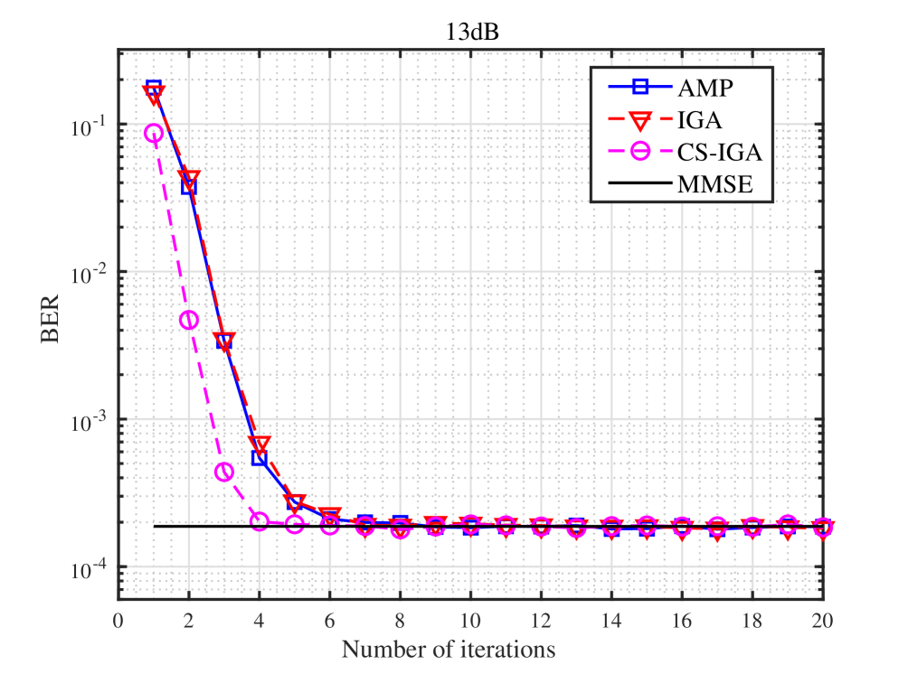
Figure 1: BER versus iteration number for different approaches at SNR=13dB under 16QAM modulation.

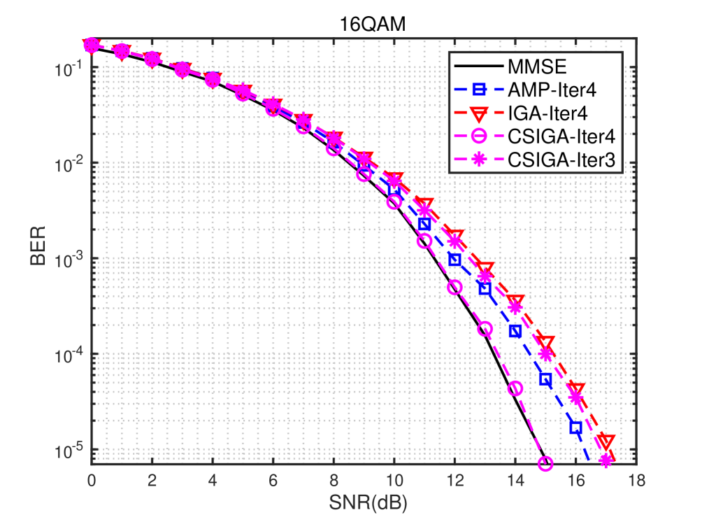
Figure 2: BER versus SNR for different approaches at 3 and 4 iterations under 16QAM modulation.

Under 64‑QAM modulation, Fig. 3 and Fig. 4 show the convergence and BER performance of the three detectors. From Fig. 3, CS‑IGA converges faster than AMP and IGA. At BER $=10^{-3}$, it requires one fewer iteration than either AMP or IGA. In Fig. 4, with the same iteration count, CS‑IGA achieves the best BER performance and most closely matches the MMSE bound. Furthermore, the BER of CS‑IGA at 5 iterations outperforms that of AMP and IGA at 6 iterations. At BER $=10^{-5}$, CS-IGA gains approximately 1.2 dB over AMP and 2 dB over IGA. We also observe that, compared to 16‑QAM, all iterative methods require more iterations to converge under 64‑QAM. These linear‑scheme results were first reported in our conference paper.

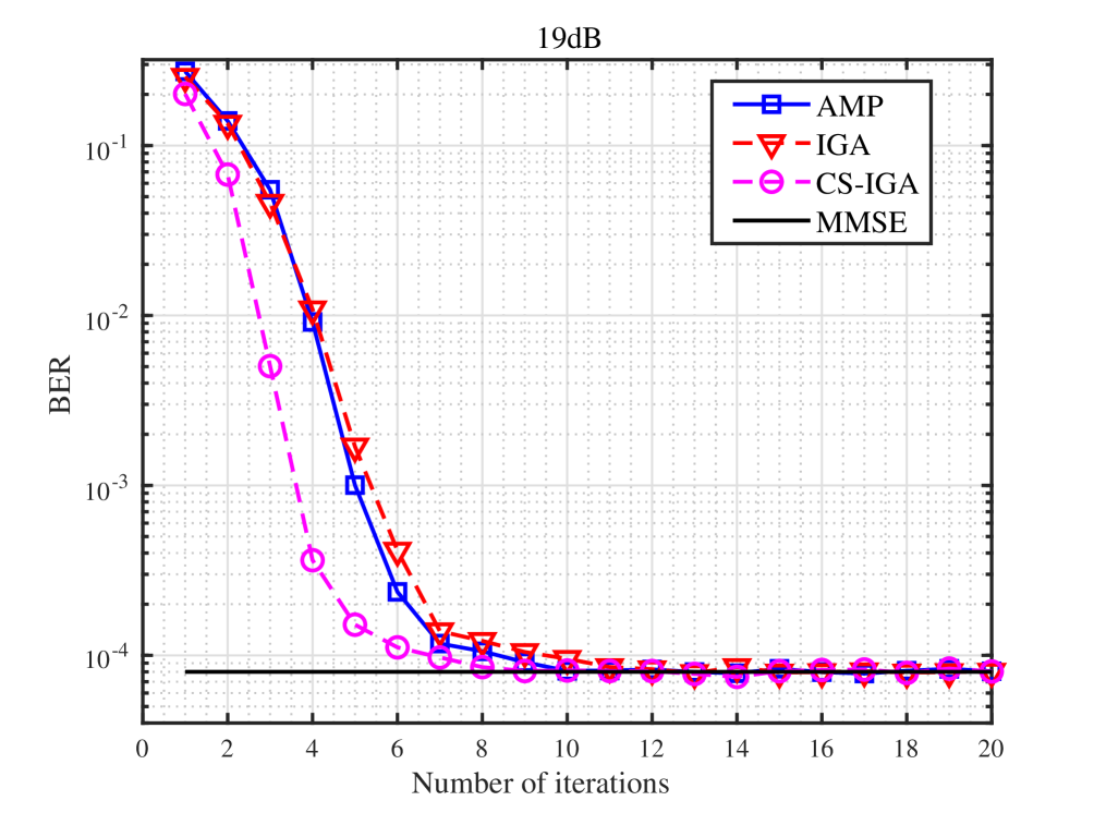
Figure 3: BER versus iteration number for different approaches at SNR=19dB under 64QAM modulation.

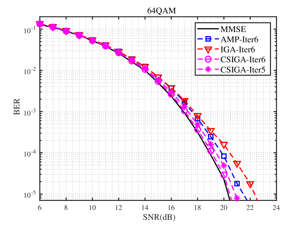
Figure 4: BER versus SNR for different approaches at 5 and 6 iterations under 64QAM modulation.

V-C Performance of the NCS-IGA

Next, we present the convergence and BER performance of NCS‑IGA compared to the Bayes‑optimal AMP, the conventional IGA, and EP in the non‑linear detection scheme. The modulation formats are QPSK, 16‑QAM, and 64‑QAM. All methods compute LLRs and then perform LDPC decoding. Fig. 5 shows the convergence behavior of NCS-IGA at SNR = 5 dB under QPSK. From this figure, we observe that both NCS‑IGA and EP converge in 2 iterations and achieve the lowest BER, while AMP and IGA require about 3 iterations. At BER = $10^{-5}$, NCS‑IGA saves one iteration compared to AMP and IGA. Notably, all of these iterative non‑linear detectors outperform the LMMSE bound. Fig. 6 shows the BER versus SNR at 1 and 2 iterations: at the same iteration counts, NCS‑IGA and EP deliver the best BER performance, and at BER = $10^{-5}$ NCS‑IGA gains approximately 0.7 dB over AMP and IGA.

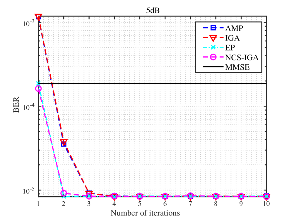
Figure 5: BER versus iteration number for different approaches at SNR=5dB under QPSK modulation.

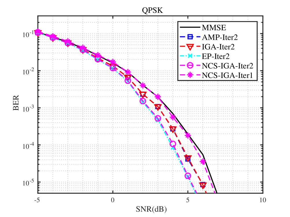
Figure 6: BER versus SNR for different approaches at 2 and 1 iterations under QPSK modulation.

The convergence and BER performance of NCS-IGA under 16-QAM modulation are shown in Fig. 7 and Fig. 8. In Fig. 7, EP converges in 2 iterations, while NCS‑IGA, IGA, and Bayes‑optimal AMP each require about 5 iterations. For iteration counts below 5, NCS‑IGA achieves a clear BER advantage over both AMP and IGA. Fig. 8 shows that, at the same iteration count, NCS‑IGA have comparable BER performance with AMP and IGA.

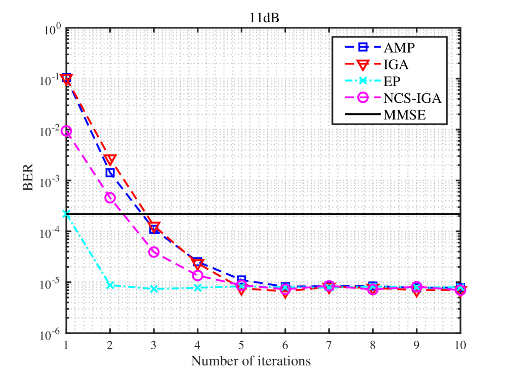
Figure 7: BER versus iteration number for different approaches at SNR=11dB under 16-QAM modulation.

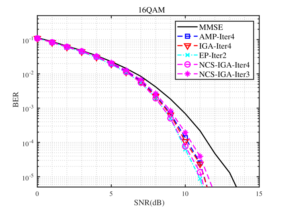
Figure 8: BER versus SNR for different approaches at 4 and 3 iterations under 16-QAM modulation.

Under 64-QAM modulation (Fig. 9 and Fig. 10), EP converges in approximately 4 iterations, whereas NCS-IGA, IGA, and AMP each need around 9 iterations. In Fig. 10, at low SNR all four methods yield nearly identical BER; at high SNR, AMP converges slightly faster than NCS-IGA and IGA. At BER $=10^{-5}$ and 6 iterations, NCS-IGA incurs about a 0.5 dB loss relative to AMP.

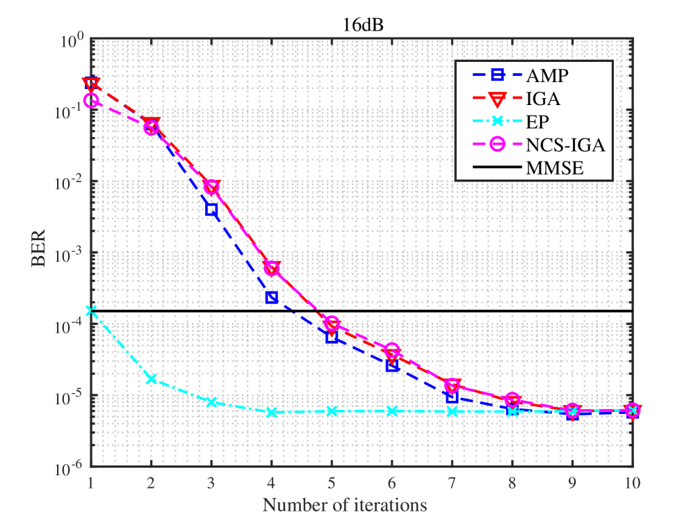
Figure 9: BER versus iteration number for different approaches at SNR=16dB under 64-QAM modulation.

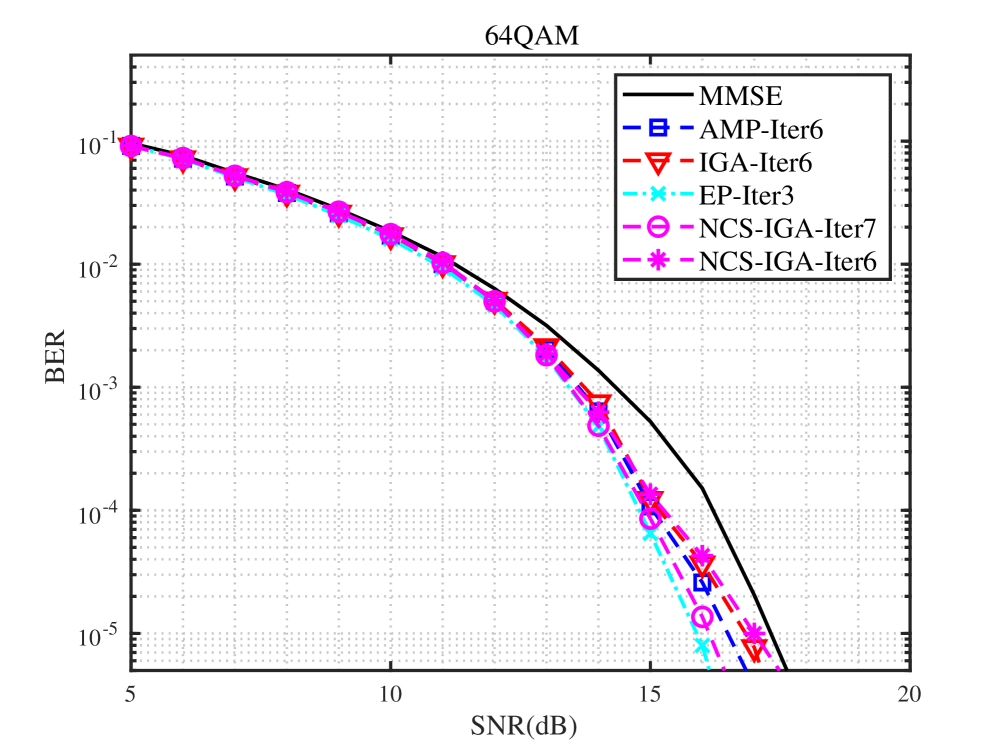
Figure 10: BER versus SNR for different approaches at 7 and 6 iterations under 64-QAM modulation.

VI Conclusion

In this paper, we have addressed the critical challenge of high-complexity signal detection in uplink XL-MIMO systems. We introduced a novel iterative detector, the CS-IGA, designed to achieve both low computational cost and rapid convergence. We further extended our method to handle discrete constellations in the nonlinear CS-IGA variant NCS-IGA. By integrating the symbol-wise moment matching directly into the geometric framework, NCS-IGA efficiently approximates the marginal a posteriori probabilities without requiring external processing loops. Our simulation results, conducted using realistic 3GPP channel models, have validated the theoretical benefits of our approach. Both CS-IGA and NCS-IGA consistently demonstrated faster convergence and matched or exceeded the BER performance of state-of-the-art AMP and IGA detectors, while operating at a fraction of the computational cost.

Appendix A Proof of Theorem 1

From the relationship between $\boldsymbol{\Theta}_{n}$ and $\boldsymbol{\Lambda}_{n}$ in (31a) , and the transform from natural parameters to expectation parameters in (13) and (14), we have the following equation

$$\mathbf{P}_{1n}\boldsymbol{\Sigma}_{n}\mathbf{P}_{1n}^{H} =-\mathbf{P}_{1n}\boldsymbol{\Theta}_{n}^{-1}\mathbf{P}_{1n}^{H},$$ (110)

$$=(\mathbf{P}_{1n}(\boldsymbol{\Lambda}_{n}+\mathbf{C}_{n}+\mathbf{D})\mathbf{P}_{1n}^{H})^{-1},$$

$$=\left(\begin{array}[]{cc}d_{n}+\Lambda_{n}&\bar{\mathbf{k}}_{n}^{H}\\ \bar{\mathbf{k}}_{n}&\bar{\mathbf{D}}_{n}+\bar{\boldsymbol{\Lambda}}_{n}\end{array}\right)^{-1},$$

Using the block matrix inversion lemma, the inversion is calculated as

$$\mathbf{P}_{1n}\boldsymbol{\Sigma}_{n}\mathbf{P}_{1n}^{H}=\left[\begin{array}[]{cc}r_{n}&\mathbf{m}_{n}^{H}\\ \mathbf{m}_{n}&\mathbf{J}_{n}\end{array}\right],$$ (113)

where $r_{n}$ and $\mathbf{m}_{n}$ are denoted by

$$r_{n}=(\Lambda_{n}+d_{n}-\bar{\mathbf{k}}_{n}^{H}\check{\boldsymbol{\Lambda}}_{n}\bar{\mathbf{k}}_{n})^{-1},$$ (114a)

$$\mathbf{m}_{n}=-{r_{n}}\check{\boldsymbol{\Lambda}}_{n}\bar{\mathbf{k}}_{n},$$ (115a)

and $\mathbf{J}_{n}$ is expressed as

$$\mathbf{J}_{n}=\left(\check{\boldsymbol{\Lambda}}_{n}^{-1}-\frac{1}{(\Lambda_{n}+d_{n})}\bar{\mathbf{k}}_{n}\bar{\mathbf{k}}_{n}^{H}\right)^{-1}.$$ (116)

Since $\bar{\mathbf{k}}_{n}\bar{\mathbf{k}}_{n}^{H}$ is a rank-1 matrix, the inversion can be easily obtained by Sherman-Morrison formula as

$$\mathbf{J}_{n} =\check{\boldsymbol{\Lambda}}_{n}+\frac{\frac{1}{(\Lambda_{n}+d_{n})}\check{\boldsymbol{\Lambda}}_{n}\bar{\mathbf{k}}_{n}\bar{\mathbf{k}}_{n}^{H}\check{\boldsymbol{\Lambda}}_{n}}{1-\frac{1}{(\Lambda_{n}+d_{n})}\bar{\mathbf{k}}_{n}^{H}\check{\boldsymbol{\Lambda}}_{n}\bar{\mathbf{k}}_{n}},$$ (117)

$$=\check{\boldsymbol{\Lambda}}_{n}+{r_{n}}\check{\boldsymbol{\Lambda}}_{n}\bar{\mathbf{k}}_{n}\bar{\mathbf{k}}_{n}^{H}\check{\boldsymbol{\Lambda}}_{n}.$$

Then, $\mathbf{P}_{1n}\boldsymbol{\Sigma}_{n}\mathbf{P}_{1n}^{H}$ can be written as

$$\mathbf{P}_{1n}\boldsymbol{\Sigma}_{n}\mathbf{P}_{1n}^{H}=\left[\begin{array}[]{cc}r_{n}&\mathbf{m}_{n}^{H}\\ \mathbf{m}_{n}&\check{\boldsymbol{\Lambda}}_{n}+{r_{n}}\check{\boldsymbol{\Lambda}}_{n}\bar{\mathbf{k}}_{n}\bar{\mathbf{k}}_{n}^{H}\check{\boldsymbol{\Lambda}}_{n}\end{array}\right].$$ (120)

Then we calculate $\mathbf{P}_{1n}\boldsymbol{\mu}_{n}$ based on $\mathbf{P}_{1n}\boldsymbol{\Sigma}_{n}\mathbf{P}_{1n}^{H}$. Based on (14), $\boldsymbol{\mu}_{n}$ is easily obtained by

$$\mathbf{P}_{1n}\boldsymbol{\mu}_{n} =\mathbf{P}_{1n}\boldsymbol{\Sigma}_{n}(\boldsymbol{\lambda}_{n}+\mathbf{b}_{n}),$$ (121)

$$=(\boldsymbol{\Lambda}_{n}+\mathbf{D}+\mathbf{C}_{n})^{-1}(\boldsymbol{\lambda}_{n}+\mathbf{b}_{n}),$$

$$=\begin{bmatrix}r_{n}&\mathbf{m}_{n}^{H}\\ \mathbf{m}_{n}&\mathbf{J}_{n}\end{bmatrix}\begin{bmatrix}\lambda_{n}+\frac{1}{\sigma_{z}^{2}}\mathbf{h}_{n}^{H}\mathbf{y}\\ \bar{\boldsymbol{\lambda}}_{n}\end{bmatrix}.$$

The $n-$th element of $\boldsymbol{\mu}_{n}$ is calculated as

$$\mu_{n} =r_{n}(\lambda_{n}+r_{n}\frac{1}{\sigma_{z}^{2}}\mathbf{h}_{n}^{H}\mathbf{y})+\mathbf{m}_{n}^{H}\bar{\boldsymbol{\lambda}}_{n},$$ (122)

$$=\frac{r_{n}}{\sigma_{z}^{2}}\mathbf{h}_{n}^{H}\mathbf{y}+r_{n}\lambda_{n}-r_{n}\bar{\mathbf{k}}_{n}^{H}\check{\boldsymbol{\Lambda}}_{n}^{H}\bar{\boldsymbol{\lambda}}_{n}.$$

Notice that $\check{\boldsymbol{\Lambda}}_{n}$ is a real diagonal matrix, so $\check{\boldsymbol{\Lambda}}_{n}^{H}=\check{\boldsymbol{\Lambda}}_{n}$. For simplicity, we define $v_{n}=\bar{\mathbf{k}}_{n}^{H}\check{\boldsymbol{\Lambda}}_{n}\bar{\boldsymbol{\lambda}}_{n}$, then $\mu_{n}$ is rewritten as

$$\mu_{n}=r_{n}\frac{1}{\sigma_{z}^{2}}\mathbf{h}_{n}^{H}\mathbf{y}+r_{n}\lambda_{n}-r_{n}v_{n}.$$ (123)

The rest elements $\bar{\boldsymbol{\mu}}_{n}$ are calculated as

$$\hskip-10.0pt\bar{\boldsymbol{\mu}}_{n} =\mathbf{m}_{n}(\lambda_{n}+\frac{1}{\sigma_{z}^{2}}\mathbf{h}_{n}^{H}\mathbf{y})+\mathbf{J}_{n}\bar{\boldsymbol{\lambda}}_{n},$$ (124)

$$=-r_{n}\frac{1}{\sigma_{z}^{2}}\check{\boldsymbol{\Lambda}}_{n}\bar{\mathbf{k}}_{n}\mathbf{h}_{n}^{H}\mathbf{y}-r_{n}\check{\boldsymbol{\Lambda}}_{n}\bar{\mathbf{k}}_{n}\lambda_{n}$$

$$~~+\check{\boldsymbol{\Lambda}}_{n}\bar{\boldsymbol{\lambda}}_{n}+r_{n}\check{\boldsymbol{\Lambda}}_{n}\bar{\mathbf{k}}_{n}\bar{\mathbf{k}}_{n}^{H}\check{\boldsymbol{\Lambda}}_{n}\bar{\boldsymbol{\lambda}}_{n},$$

$$=-\check{\boldsymbol{\Lambda}}_{n}\bar{\mathbf{k}}_{n}(\frac{r_{n}}{\sigma_{z}^{2}}\mathbf{h}_{n}^{H}\mathbf{y}+r_{n}\lambda_{n}-r_{n}\bar{\mathbf{k}}_{n}^{H}\check{\boldsymbol{\Lambda}}_{n}\bar{\boldsymbol{\lambda}}_{n})+\check{\boldsymbol{\Lambda}}_{n}\bar{\boldsymbol{\lambda}}_{n},$$

$$=-\mu_{n}\check{\boldsymbol{\Lambda}}_{n}\bar{\mathbf{k}}_{n}+\check{\boldsymbol{\Lambda}}_{n}\bar{\boldsymbol{\lambda}}_{n}.$$

Then $\mathbf{P}_{1n}\boldsymbol{\mu}_{n}$ is denoted as

$$\mathbf{P}_{1n}\boldsymbol{\mu}_{n}=\begin{bmatrix}\mu_{n}\\ \bar{\boldsymbol{\mu}}_{n}\end{bmatrix}=\left[\begin{array}[]{c}\frac{r_{n}}{\sigma_{z}^{2}}\mathbf{h}_{n}^{H}\mathbf{y}+r_{n}\lambda_{n}-r_{n}v_{n}\\ -\mu_{n}\check{\boldsymbol{\Lambda}}_{n}\bar{\mathbf{k}}_{n}+\check{\boldsymbol{\Lambda}}_{n}\bar{\boldsymbol{\lambda}}_{n}\end{array}\right].$$ (127)

This complete the proof.

Appendix B Proof of Theorem 2

Upon convergence, the algorithm satisfies both the $e$- and $m$-conditions, the relationship of expectation parameters at the fixed point is given by (83a) and (84a), which leads to

$$\sum_{n=1}^{N}\boldsymbol{\lambda}_{n}^{\bullet} =(N-1)\boldsymbol{\lambda}_{0}^{\bullet},$$ (128a)

$$\sum_{n=1}^{N}\boldsymbol{\Lambda}_{n}^{\bullet} =(N-1)\boldsymbol{\Lambda}_{0}^{\bullet}.$$ (129a)

Considering $\boldsymbol{\mu}_{n}$ satisfies

$$\boldsymbol{\mu}_{n} =-\boldsymbol{\Theta}_{n}^{-1}\boldsymbol{\theta}_{n}$$ (130)

$$=(\boldsymbol{\Lambda}_{n}+\mathbf{C}_{n}+\mathbf{D})^{-1}(\boldsymbol{\lambda}_{n}+\mathbf{b}_{n}).$$

By taking sum over natural parameters of all AMs, we have the following property

$$\sum_{n=1}^{N}\boldsymbol{\lambda}_{n}^{\bullet} =\sum_{n=1}^{N}(\boldsymbol{\Lambda}_{n}^{\bullet}+\mathbf{C}_{n}+\mathbf{D})\boldsymbol{\mu}^{\bullet}-\sum_{n=1}^{N}\mathbf{b}_{n},$$ (131)

$$=\left(\sum_{n=1}^{N}\boldsymbol{\Lambda}_{n}^{\bullet}+\mathbf{K}-\mathbf{I}\odot\mathbf{K}+\mathbf{D}\right)\boldsymbol{\mu}^{\bullet}-\mathbf{H}^{H}\mathbf{y},$$

$$=\left(\sum_{n=1}^{N}\boldsymbol{\Lambda}_{n}^{\bullet}+\mathbf{K}+\mathbf{I}\right)\boldsymbol{\mu}^{\bullet}-\mathbf{H}^{H}\mathbf{y}$$

where $\mathbf{K}=\sigma_{z}^{-2}\mathbf{H}^{H}\mathbf{H}$. Substituting (128a) into (131), we have

$$(N-1)\boldsymbol{\lambda}_{0}^{\bullet}=(N-1)\boldsymbol{\Lambda}_{0}^{\bullet}\boldsymbol{\mu}^{\bullet}+(\mathbf{K}+\mathbf{I})\boldsymbol{\mu}^{\bullet}-\mathbf{H}^{H}\mathbf{y}.$$ (132)

Since $\boldsymbol{\mu}^{\bullet}=(\boldsymbol{\Lambda}_{0}^{\bullet})^{-1}\boldsymbol{\lambda}^{\bullet}$, (132) can be rewritten as

$$\mathbf{H}^{H}\mathbf{y}=(\mathbf{K}+\mathbf{I})\boldsymbol{\mu}^{\bullet}.$$ (133)

Then $\boldsymbol{\mu}^{\bullet}$ is obtained by

$$\boldsymbol{\mu}^{\bullet} =(\mathbf{K}+\mathbf{I})^{-1}\mathbf{H}^{H}\mathbf{y},$$ (134)

$$=(\sigma_{z}^{-2}\mathbf{H}^{H}\mathbf{H}+\mathbf{I})^{-1}\mathbf{H}^{H}\mathbf{y},$$

which is equivalent to the a posteriori mean in (3a) or the LMMSE mean. This complete the proof.

References

• [1] T. L. Marzetta, “Noncooperative cellular wireless with unlimited numbers of base station antennas,” IEEE Trans. Wireless Commun., vol. 9, no. 11, pp. 3590–3600, 2010.
• [2] J. Hoydis, S. ten Brink, and M. Debbah, “Massive MIMO in the UL/DL of cellular networks: How many antennas do we need?” IEEE J. Sel. Areas Commun., vol. 31, no. 2, pp. 160–171, 2013.
• [3] L. Lu, G. Y. Li, A. L. Swindlehurst, A. Ashikhmin, and R. Zhang, “An overview of massive MIMO: Benefits and challenges,” IEEE J. Sel. Topics Signal Process., vol. 8, no. 5, pp. 742–758, 2014.
• [4] E. Björnson, J. Hoydis, M. Kountouris, and M. Debbah, “Massive MIMO systems with non-ideal hardware: Energy efficiency, estimation, and capacity limits,” IEEE Trans. Inf. Theory, vol. 60, no. 11, pp. 7112–7139, 2014.
• [5] E. De Carvalho, A. Ali, A. Amiri, M. Angjelichinoski, and R. W. Heath, “Non-stationarities in extra-large-scale massive MIMO,” IEEE Wireless Commun., vol. 27, no. 4, pp. 74–80, 2020.
• [6] M. Alsabah, M. A. Naser, B. M. Mahmmod, S. H. Abdulhussain, M. R. Eissa, A. Al-Baidhani, N. K. Noordin, S. M. Sait, K. A. Al-Utaibi, and F. Hashim, “6G wireless communications networks: A comprehensive survey,” IEEE Access, vol. 9, pp. 148 191–148 243, 2021.
• [7] Z. Wang, J. Zhang, H. Du, D. Niyato, S. Cui, B. Ai, M. Debbah, K. B. Letaief, and H. V. Poor, “A tutorial on extremely large-scale MIMO for 6G: Fundamentals, signal processing, and applications,” IEEE Commun. Surveys Tuts., vol. 26, no. 3, pp. 1560–1605, 2024.
• [8] 3GPP, “TS 38.300: NR; NR and NG-RAN overall description; stage-2,” 3rd Generation Partnership Project, Tech. Rep., 2023.
• [9] C.-X. Wang, X. You, X. Gao, X. Zhu, Z. Li, C. Zhang, H. Wang, Y. Huang, Y. Chen, H. Haas, J. S. Thompson, E. G. Larsson, M. D. Renzo, W. Tong, P. Zhu, X. Shen, H. V. Poor, and L. Hanzo, “On the road to 6G: Visions, requirements, key technologies, and testbeds,” IEEE Commun. Surveys Tuts., vol. 25, no. 2, pp. 905–974, 2023.
• [10] S. Yang and L. Hanzo, “Fifty years of MIMO detection: The road to large-scale MIMOs,” IEEE Commun. Surveys Tuts., vol. 17, no. 4, pp. 1941–1988, 2015.
• [11] M. A. Albreem, M. Juntti, and S. Shahabuddin, “Massive MIMO detection techniques: A survey,” IEEE Commun. Surveys Tuts., vol. 21, no. 4, pp. 3109–3132, 2019.
• [12] H. Prabhu, J. Rodrigues, O. Edfors, and F. Rusek, “Approximative matrix inverse computations for very-large MIMO and applications to linear pre-coding systems,” in Proc. IEEE Wireless Commun. Netw. Conf. (WCNC), 2013, pp. 2710–2715.
• [13] C. Tang, C. Liu, L. Yuan, and Z. Xing, “High precision low complexity matrix inversion based on Newton iteration for data detection in the massive MIMO,” IEEE Commun. Lett., vol. 20, no. 3, pp. 490–493, 2016.
• [14] B. Y. Kong and I.-C. Park, “Low-complexity symbol detection for massive MIMO uplink based on Jacobi method,” in Proc. IEEE Annu. Int. Symp. Pers. Indoor Mobile Radio Commun. (PIMRC), 2016, pp. 1–5.
• [15] L. Dai, X. Gao, X. Su, S. Han, C.-L. I, and Z. Wang, “Low-complexity soft-output signal detection based on gauss–seidel method for uplink multiuser large-scale mimo systems,” IEEE Transactions on Vehicular Technology, vol. 64, no. 10, pp. 4839–4845, 2015.
• [16] B. Yin, M. Wu, J. R. Cavallaro, and C. Studer, “Conjugate gradient-based soft-output detection and precoding in massive MIMO systems,” in Proc. IEEE Global Commun. Conf. (GLOBECOM), 2014, pp. 3696–3701.
• [17] T. Takahashi, A. Tölli, S. Ibi, and S. Sampei, “Low-complexity large MIMO detection via layered belief propagation in beam domain,” IEEE Trans. Wireless Commun., vol. 21, no. 1, pp. 234–249, 2022.
• [18] J. Céspedes, P. M. Olmos, M. Sánchez-Fernández, and F. Perez-Cruz, “Expectation propagation detection for high-order high-dimensional MIMO systems,” IEEE Trans. Commun., vol. 62, no. 8, pp. 2840–2849, 2014.
• [19] M. J. Beal, Variational Algorithms for Approximate Bayesian Inference, 2003.
• [20] D. L. Donoho, A. Maleki, and A. Montanari, “Message passing algorithms for compressed sensing: I. motivation and construction,” in Proc. IEEE Inf. Theory Workshop (ITW), 2010, pp. 1–5.
• [21] J. Ma and L. Ping, “Orthogonal AMP,” IEEE Access, vol. 5, pp. 2020–2033, 2017.
• [22] S. Rangan, P. Schniter, and A. K. Fletcher, “Vector approximate message passing,” IEEE Trans. Inf. Theory, vol. 65, no. 10, pp. 6664–6684, 2019.
• [23] L. Liu, S. Huang, and B. M. Kurkoski, “Memory AMP,” IEEE Trans. Inf. Theory, vol. 68, no. 12, pp. 8015–8039, 2022.
• [24] S. Ikeda, T. Tanaka, and S. Amari, “Information geometry of turbo and low-density parity-check codes,” IEEE Trans. Inf. Theory, vol. 50, no. 6, pp. 1097–1114, 2004.
• [25] J. Yang, A.-A. Lu, Y. Chen, X. Gao, X.-G. Xia, and D. T. Slock, “Channel estimation for massive MIMO: An information geometry approach,” IEEE Trans. Signal Process., vol. 70, pp. 4820–4834, 2022.
• [26] J. Yang, Y. Chen, X. Gao, D. T. Slock, and X.-G. Xia, “Signal detection for ultra-massive MIMO: An information geometry approach,” IEEE Trans. Signal Process., vol. 72, pp. 824–838, 2024.
• [27] J. Yang, Y. Chen, A.-A. Lu, W. Zhong, X. Gao, X. You, X.-G. Xia, and D. Slock, “Channel estimation for massive MIMO-OFDM: Simplified information geometry approach,” in Proc. IEEE Veh. Technol. Conf. (VTC), 2023, pp. 1–6.
• [28] B. Liu, A.-A. Lu, M. Fan, J. Yang, and X. Gao, “An information geometry interpretation for approximate message passing,” arXiv preprint arXiv:2408.06907, 2024.
• [29] A.-A. Lu, B. Liu, and X. Gao, “Interference cancellation information geometry approach for massive MIMO channel estimation,” arXiv preprint arXiv:2406.19583, 2024.
• [30] V. C. Rodrigues, A. Amiri, T. Abrão, E. de Carvalho, and P. Popovski, “Low-complexity distributed xl-mimo for multiuser detection,” in Proc. IEEE Int. Conf. Commun. Workshops (ICC Workshops), 2020, pp. 1–6.
• [31] K. Zhi, C. Pan, H. Ren, K. K. Chai, C.-X. Wang, R. Schober, and X. You, “Xl-mimo with near-field spatial non-stationarities: Low-complexity detector design,” in Proc. IEEE Global Commun. Conf. (GLOBECOM), 2023, pp. 7194–7199.
• [32] S. M. Kay, Fundamentals of Statistical Signal Processing, Volume I: Estimation Theory.   Upper Saddle River, NJ, USA: Prentice Hall, 1993.
• [33] S.-i. Amari, Information Geometry and Its Applications.   Tokyo: Springer, 2016.
• [34] S. Nam, J. Kim, and Y. Han, “A user selection algorithm using angle between subspaces for downlink MU-MIMO systems,” IEEE Trans. Commun., vol. 62, no. 2, pp. 616–624, 2014.
• [35] S. Jaeckel, L. Raschkowski, K. Börner, and L. Thiele, “Quadriga: A 3-D multi-cell channel model with time evolution for enabling virtual field trials,” IEEE Trans. Antennas Propag., vol. 62, no. 6, pp. 3242–3256, 2014.