Soft Guessing Under Logarithmic Loss Allowing Errors and Variable-Length Source Coding

Abstract

This paper considers the problem of soft guessing under a logarithmic loss distortion measure while allowing errors. We find an optimal guessing strategy, and derive single-shot upper and lower bounds for the minimal guessing moments as well as an asymptotic expansion for i.i.d. sources. These results are extended to the case where side information is available to the guesser. Furthermore, a connection between soft guessing allowing errors and variable-length lossy source coding under logarithmic loss is demonstrated. The Rényi entropy, the smooth Rényi entropy, and their conditional versions play an important role.

I Introduction

In 1994, Massey [4] introduced the information-theoretic study of guessing, or guesswork, and considered the following basic problem: a guesser seeks to determine the value of a random variable $X$, taking values in $\mathcal{X}=\{1,2,\ldots,|\mathcal{X}|\}$, by asking questions of the form: “is $X$ equal to $x_{1}$?”, “is $X$ equal to $x_{2}$?” and so on. An honest answer is returned for each query, and guessing continues until the answer is “yes”. Such a guessing strategy is specified by a permutation of $\mathcal{X}$, and is denoted henceforth as $\mathcal{G}=(x_{1},x_{2},\ldots,x_{|\mathcal{X}|})$. Any guessing strategy induces a bijective function $g:\mathcal{X}\to\{1,\ldots,|\mathcal{X}|\}$, where $g(x)$ is the guessing order of $x$, i.e., the number of guesses required when $X=x$. Massey [4] investigated the relationship between the expected number of guesses, minimized over all guessing strategies, and the Shannon entropy.

Two years later, Arıkan [5] considered the more general problem of studying the minimal $\rho$-th guessing moment, defined for every $\rho>0$ as

$$M^{\star}_{X}(\rho):=\min_{\mathcal{G}}\mathbb{E}\left[g(X)^{\rho}\right]=\min_{\mathcal{G}}\sum_{x\in\mathcal{X}}P_{X}(x)g(x)^{\rho},$$ (1)

where $P_{X}$ is the probability mass function (pmf) of $X$. Arıkan showed that all guessing moments are simultaneously minimized by a strategy that queries realizations in a decreasing order of their probability, and derived bounds on $M^{\star}_{X}(\rho)$ given by

$$M^{\star}_{X}(\rho)\leq\exp\left(\rho H_{\frac{1}{1+\rho}}(X)\right)$$ (2)

and

$$M^{\star}_{X}(\rho)\geq\left(1+\log|\mathcal{X}|\right)^{-\rho}\exp\left(\rho H_{\frac{1}{1+\rho}}(X)\right),$$ (3)

where $H_{\frac{1}{1+\rho}}(X)$ is the Rényi entropy of order $1/(1+\rho)$ [6] (see Section II-A). Together, (2) and (3) provide a tight exponential characterization of the guessing moment (known as the guessing exponent) in the i.i.d. asymptotic regime, where the task is to guess an $n$-vector $X^{n}=X_{1},\ldots,X_{n}$ of i.i.d. entries. Arıkan further generalized the problem to the case where a correlated side information random variable is available to the guesser, establishing a connection to the Arimoto-Rényi conditional entropy [7]; and applied this result to study the computational complexity and cutoff rate of sequential decoding.

Since the works of Massey and Arıkan, the original guessing problem has been extended and studied in various contexts, including: guessing subject to distortion [8, 9, 10, 11, 12], guessing allowing errors [13, 14], guessing under source uncertainty [15], guessing and large deviations [16, 17, 18, 19, 20], guessing and joint source-channel coding [21], guessing via an unreliable oracle [22], guessing with limited memory [23], guessing for Markov sources [24], multi-agent guesswork [25, 26], guesswork of hash functions [27], multi-user guesswork [28], guesswork subject to a per-symbol Shannon entropy budget [29], universal randomized guessing [9, 30], guessing based on compressed side information [31], guessing individual sequences [32], guesses transmitted via a noisy channel [33], multiple guesses under a tunable loss function [34], improved bounds and connections to variable-length source coding [35], and connections to majorization theory [36], among others. Guessing has also played a key role in analyzing a channel decoding paradigm that queries noise patterns instead of codewords, known as GRAND [37, 38, 39, 40].

Of particular interest to our current work are two extensions of the original Massey-Arıkan guessing settings: the first is the guessing allowing errors problem proposed by Kuzuoka [13], and the second is the soft guessing under log-loss problem proposed by Wu and Joudeh [12]. Next, we briefly review these two problems.

I-A Guessing Allowing Errors

In Kuzuoka’s guessing allowing errors framework, the guesser may stop guessing and declare an error at any step [13]. In particular, at the $i$-th step, the guesser gives up guessing and declares an error with probability $\pi_{i}$ or continues guessing with probability $1-\pi_{i}$, where $0\leq\pi_{i}\leq 1$. A guessing strategy is specified by a pair $(\mathcal{G},\pi)$, where $\mathcal{G}$ is as defined earlier, inducing a guessing function $g$, while $\pi=(\pi_{1},\pi_{2},\ldots,\pi_{|\mathcal{X}|})$ is a sequence of give up probabilities. For a fixed strategy, let

$$\lambda_{i}:=\prod_{j=1}^{i}(1-\pi_{j})$$ (4)

for $i=1,2,\ldots,|\mathcal{X}|$, i.e., $\lambda_{i}$ is the probability that the guesser does not give up guessing before making the $i$-th guess. Such a randomized guessing strategy gives rise to a stochastic guessing function $G:\mathcal{X}\to\{1,\ldots,|\mathcal{X}|\}\cup\{0\}$ defined as

$$G(x):=\begin{cases}g(x),&\mathrm{with~probability}~\lambda_{g(x)},\\ 0,&\mathrm{with~probability}~1-\lambda_{g(x)}.\end{cases}$$ (5)

Note that $G(x)=0$ represents the event that the guesser gives up before asking the question “is $X$ equal to $x$?”. The probability that $X$ is correctly guessed at the $i$-th step before giving up is hence $\mathbb{P}\left[G(X)=i\right]=\lambda_{i}P_{X}\big(g^{-1}(i)\big)$. On the other hand, the probability that the guesser gives up before correctly guessing $X$, i.e., error probability, is given by

$$P_{e}:=\mathbb{P}\left[G(X)=0\right]=1-\sum_{i=1}^{|\mathcal{X}|}\lambda_{i}P_{X}\big(g^{-1}(i)\big).$$ (6)

Therefore, the $\rho$-th guessing moment in this case is defined as

$$M_{X}(\rho,\mathcal{G},\pi):=\mathbb{E}\left[G(X)^{\rho}\right]=\sum_{i=1}^{|\mathcal{X}|}\lambda_{i}P_{X}\big(g^{-1}(i)\big)\times i^{\rho}.$$ (7)

Naturally, there is a trade-off between $M_{X}(\rho,\mathcal{G},\pi)$ and $P_{e}$, e.g., the former can be made arbitrarily small by making $P_{e}$ large enough. Under the constraint that $P_{e}$ must not exceed $\epsilon$, the minimal $\rho$-th guessing moment is defined as

$$M_{X}^{\star}(\rho,\epsilon):=\min_{\mathcal{G},\pi:P_{e}\leq\epsilon}M_{X}(\rho,\mathcal{G},\pi).$$ (8)

Mirroring Arıkan’s bounds in (2) and (3), Kuzuoka [13] showed that $M_{X}^{\star}(\rho,\epsilon)$ is bounded as

$$M^{\star}_{X}(\rho,\epsilon)\leq\exp\left(\rho H_{\frac{1}{1+\rho}}^{\epsilon}(X)\right)$$ (9)

and

$$M^{\star}_{X}(\rho,\epsilon)\geq\left(1+\log|\mathcal{X}|\right)^{-\rho}\exp\left(\rho H_{\frac{1}{1+\rho}}^{\epsilon}(X)\right),$$ (10)

where $H_{\frac{1}{1+\rho}}^{\epsilon}(X)$ denotes the $\epsilon$-smooth Rényi entropy, introduced by Renner and Wolf [41] (see Section II-B). The bounds in (9) and (10) provide a tight exponential characterization of guessing moments in the i.i.d. asymptotic regime. Interestingly, the guessing exponent in this case is characterized in terms of the Shannon entropy for any $\epsilon\in(0,1)$, a consequence of the smooth Rényi entropy’s asymptotic properties [14]. Kuzuoka also proposed an $\epsilon$-smooth counterpart to the Arimoto-Rényi conditional entropy [13], and employed it to bound the $\rho$-th guessing moment for the side information variant of the problem.

I-B Soft Guessing Under Log-Loss

The Wu-Joudeh soft guessing paradigm [12] can be seen as a variant of guessing subject to distortion, but instead of guessing a “hard” reconstruction, i.e., a reproduction symbol $\hat{X}$ as in previous works (e.g., [8]), the guesser seeks to find a good “soft” reconstruction of $X$, i.e., a probability distribution $\hat{P}$ on the alphabet $\mathcal{X}$. The fidelity of the soft reconstruction is measured by the logarithmic loss (log-loss) [42, 43, 44], defined for every symbol $x\in\mathcal{X}$ and soft reconstruction $\hat{P}$ as

$$d(x,\hat{P}):=\log\frac{1}{\hat{P}(x)}.$$ (11)

A soft guessing strategy is specified by a sequence $\mathcal{G}_{\mathrm{soft}}=(\hat{P}_{1},\hat{P}_{2},\ldots,\hat{P}_{N})$ of $N$ probability distributions on $\mathcal{X}$, for some integer $N$. The guesser asks questions of the form: “is $d(X,\hat{P}_{1})\leq D$?”, “is $d(X,\hat{P}_{2})\leq D$?” and so on until the answer is “yes”, where $D\geq 0$ is some predetermined distortion level. If the soft guessing strategy terminates with probability $1$ for a given distortion level $D$, then we call it $D$-admissible, and we denote it by $\mathcal{G}_{\mathrm{soft}}(D)$. Such a strategy induces a guessing function $g(x)$, which is the smallest index $j$ for which $d(x,\hat{P}_{j})\leq D$ is satisfied. Note that soft guessing can be reduced to standard guessing by setting $D=0$ and selecting a strategy that consists of distinct hard reconstructions, i.e., single-mass point distributions. For a given distortion level $D$, the minimal $\rho$-the soft guessing moment is defined as

$$M^{\star}_{X}(\rho,D):=\min_{\mathcal{G}_{\mathrm{soft}}(D)}\mathbb{E}\left[g(X)^{\rho}\right].$$ (12)

Wu and Joudeh [12] showed that $M^{\star}_{X}(\rho,D)$ is bounded as

$$M^{\star}_{X}(\rho,D)\leq 1+2^{\rho}\exp\left(\rho H_{\frac{1}{1+\rho}}(X)-\rho\log\lfloor\exp(D)\rfloor\right)$$ (13)

and

$$M^{\star}_{X}(\rho,D)\geq\left(1+\log|\mathcal{X}|\right)^{-\rho}\exp\left(\rho H_{\frac{1}{1+\rho}}(X)-\rho\log\lfloor\exp(D)\rfloor\right),$$ (14)

where the upper bound in (13) can be tightened to Arıkan’s upper bound in (2) whenever $0\leq D<1$ (i.e. $\lfloor\exp(D)\rfloor=1$). A tight characterization of the guessing exponent in the i.i.d. asymptotic regime can also be recovered from (13) and (14), and the result is also easily extended to the case where side information is available to the guesser.

I-C Soft Guessing Under Log-Loss Allowing Errors

In this paper, we propose a natural generalization of the above settings. Specifically, we study the problem of soft guessing under log-loss while allowing errors. In this formulation, the guesser seeks a good soft reconstruction of $X$ in the sense of Wu and Joudeh [12], while also being permitted to give up guessing and declare an error, following the framework of Kuzuoka [13]. A formal description of the setting is given in Section III. Our goal is to derive upper and lower bounds on the minimal guessing moments in this setting, which subsume all previously stated bounds as special cases.

Guessing subject to distortion is generally motivated by applications such as betting games, pattern matching, search algorithms, biometric authentication, and simple sequential rate–distortion encoding [8, 9, 10]. The soft guessing under log-loss framework is similarly motivated, but with the goal of recovering a probability distribution rather than a single point estimate, making it more consistent with a fully Bayesian perspective. Allowing errors further broadens the scope of applications, enabling scenarios where the search effort can be reduced at the cost of permitting a small error probability.

The close connection with source coding is another key motivation of this work. Bounds on guessing moments are known to yield bounds on the normalized cumulant function of codeword lengths in corresponding variable-length source coding problems (without the prefix constraint) (see, e.g., [35, 12]). Naturally, the guessing framework we propose is related to a variable-length lossy source coding problem under log-loss and allowing errors. A further goal of this paper is to derive bounds on the cumulant function of codeword lengths in this setting, thereby extending prior results for the error-free case [44, 12]. Next, we outline the organization of the paper and highlight our main technical contributions.

I-D Organization and Contributions

In Section II, we review the definitions of the Rényi entropy, smooth Rényi entropy, and their conditional variants. We also present several key properties and derive new ones that are useful in our proofs. In particular, we extend a chain rule for smooth Rényi entropy, due to Renner and Wolf [41], to the conditional case (see Lemma 7).

Section III forms the core of this paper. Here, we first formulate the problem of soft guessing under log-loss allowing errors, and then identify the optimal guessing strategy. This strategy is based on list guessing [12], augmented with a probabilistic stopping rule that allows termination after a certain number of attempts with a carefully chosen probability, similar to [13]. We then establish single-shot upper and lower bounds on the minimal soft guessing moment in terms of the smooth Rényi entropy of a derived random variable $Z$, representing the index of the list containing the original random variable $X$ (see Theorem 1). We also derive explicit bounds involving the smooth Rényi entropy of $X$ itself (see Proposition 2), resembling those in (13) and (14). These explicit bounds are instrumental in obtaining the guessing exponent in the i.i.d. asymptotic regime.

In Section IV, we extend the results of Section III to the case where side information is available to the guesser. In the resulting bounds, the smooth Rényi entropy is replaced by a conditional smooth Rényi entropy due to Kuzuoka [13]. Our new conditional chain rule in Lemma 7 is crucial for deriving the explicit lower bound on the guessing moment.

In Section V, we establish a connection between the considered guessing problem and the problem of variable-length lossy source coding under log-loss and allowing errors. We show that the minimal normalized cumulant generating function of codeword lengths is bounded above and below in terms of the minimal soft guessing moment. By using this relationship and the results in Section III, we give bounds on the minimal normalized cumulant generating function of codeword lengths in terms of the smooth Rényi entropy. Moreover, we investigate the tightness of these bounds.

I-E Basic Notations

Random variables are denoted by uppercase letters (e.g., $X$, $Y$, $Z$), while realizations of random variables are denoted by lowercase letters (e.g., $x$, $y$, $z$). The set in which a random variable takes values is denoted by the corresponding calligraphic letter, e.g., random variable $X$ takes values in the set $\mathcal{X}$. The $n$-fold Cartesian product of $\mathcal{X}$ is denoted by $\mathcal{X}^{n}$. Random variables take values in a finite set unless otherwise stated. We use conventional notations for probability mass functions (pmf), e.g., $P_{X}$, $P_{X,Y}$, and $P_{X|Y}$ denote the pmf of $X$, the joint pmf of $X,Y$, and the conditional pmf of $X$ given $Y$, respectively. The expectation operator is denoted by $\mathbb{E}[\cdot]$. The set of probability distributions on $\mathcal{X}$, i.e., probability simplex, is denoted by $\mathcal{P}(\mathcal{X})$. The cardinality of a set $\mathcal{X}$ is denoted by $|\mathcal{X}|$. For $a\in\mathbb{R}$, $\lfloor a\rfloor$ is the greatest integer less than or equal to $a$ and $\lceil a\rceil$ is the least integer greater than or equal to $a$. Throughout the paper, $\log(\cdot)$ denotes $\log_{2}(\cdot)$ and $\exp(\cdot)$ denotes $2^{(\cdot)}$.

II Preliminaries

The Rényi entropy, the smooth Rényi entropy, and their conditional versions play an important role in this paper. In this section, we present their definitions and some useful properties used in the proofs of the main theorems of this paper. As we see further on, in the context of guessing, Rényi entropy orders of most relevance are $\alpha\in(0,1)$. Hence, we assume $\alpha\in(0,1)$ throughout the paper. Moreover, we assume $\epsilon\in[0,1)$ for the smoothness parameter.

II-A Rényi Entropy and Arimoto-Rényi Conditional Entropy

The Rényi entropy of order $\alpha$ is defined as [6]

$$H_{\alpha}(X):=\frac{1}{1-\alpha}\log\sum_{x\in{\cal X}}[P_{X}(x)]^{\alpha}.$$ (15)

By using L’Hôpital’s rule, it can be shown that

$$\lim_{\alpha\to 1}H_{\alpha}(X)=H(X),$$ (16)

where $H(X)$ denotes the standard Shannon entropy. For brevity, we will use the convention $H_{1}(X)=H(X)$, where it is understood that $H_{1}(X)$ is obtained by taking the limit as in (16). For a pair of random variables $X$ and $Y$, the order-$\alpha$ Arimoto-Rényi conditional entropy of $X$ given $Y$ is defined as [7]

$$H_{\alpha}(X|Y):=\frac{\alpha}{1-\alpha}\log\left(\sum_{y\in\mathcal{Y}}\left[\sum_{x\in\mathcal{X}}[P_{X,Y}(x,y)]^{\alpha}\right]^{1/\alpha}\right).$$ (17)

As in (16), we have $H_{1}(X|Y)=H(X|Y)$, which is the Shannon conditional entropy. Moreover, it holds that

$$H_{\alpha}(X|Y)\leq H_{\alpha}(X),$$ (18)

with equality if $X$ and $Y$ are independent. It should be noted that there are several distinct suggestions for formulating the conditional Rényi entropy which serve different purposes, see, e.g., [45]. The Arimoto-Rényi version is best suited for characterizing guessing moments with side information, as shown by Arıkan [5].

II-B Smooth Rényi Entropy and Conditional Smooth Rényi Entropies

II-B1 Smooth Rényi Entropy

The smooth Rényi entropy was introduced by Renner and Wolf in [41]. The $\epsilon$-smooth Rényi entropy of order $\alpha$ is defined as

$$H^{\epsilon}_{\alpha}(X):=\frac{1}{1-\alpha}\log\left(\inf_{Q_{X}\in\mathcal{B}^{\epsilon}(P_{X})}\sum_{x\in\mathcal{X}}[Q_{X}(x)]^{\alpha}\right),$$ (19)

where $\mathcal{B}^{\epsilon}(P_{X})$ is a set of functions $Q_{X}:\mathcal{X}\rightarrow[0,1]$ such that $Q_{X}(x)\leq P_{X}(x)$ for all $x\in\mathcal{X}$ and $\sum_{x\in\mathcal{X}}Q_{X}(x)\geq 1-\epsilon$.

Remark 1.

$H^{0}_{\alpha}(X)$ is equal to the Rényi entropy $H_{\alpha}(X)$, since $Q_{X}(x)=P_{X}(x)$ for all $x\in\mathcal{X}$ when $\epsilon=0$.

For $X$ and $Y$, the joint $\epsilon$-smooth Rényi entropy of order $\alpha$ is defined in a similar manner as (19), and is denoted by $H^{\epsilon}_{\alpha}(X,Y)$. As shown in [41], certain properties satisfied by the Shannon entropy have counterparts for the smooth Rényi entropy. We present ones that are useful to us in our proofs.

Lemma 1 ([41, Lemma 7]).

For random variables $X$ and $Y$, we have

$$H^{\epsilon}_{\alpha}(X)\leq H^{\epsilon}_{\alpha}(X,Y).$$ (20)

Lemma 2 ([41, Eq. (12)]).

Let $f(X)$ be a function of $X$. Then

$$H^{\epsilon}_{\alpha}(f(X))\leq H^{\epsilon}_{\alpha}(X).$$ (21)

By setting $\epsilon=0$ in (21) and recalling Remark 1, we recover $H_{\alpha}(f(X))\leq H_{\alpha}(X)$. Moreover, setting $\alpha=1$ and recalling (16), we recover $H(f(X))\leq H(X)$, a well-known inequality for the Shannon entropy (see, e.g., [46, Problem 2.4]).

II-B2 Smooth Rényi Entropy Explicit Formula

Koga [47] showed that for orders $\alpha\in(0,1)$, the infimum in the definition of smooth Rényi entropy can be solved explicitly. For convenience, we henceforth assume without loss of generality that

$$P_{X}(1)\geq P_{X}(2)\geq\ldots\geq P_{X}(|\mathcal{X}|)>0.$$ (22)

Given $\epsilon\in[0,1)$, let $i^{*}_{X}$ be the minimum integer in $\{1,2,\ldots,|\mathcal{X}|\}$ such that

$$\sum_{k=1}^{i^{*}_{X}}P_{X}(k)\geq 1-\epsilon.$$ (23)

Furthermore, define $Q^{\epsilon}_{X}(j)$ such that

$$Q^{\epsilon}_{X}(j)=\begin{cases}P_{X}(j),&j=1,2,\ldots,i^{*}_{X}-1,\\ 1-\epsilon-\sum_{i=1}^{i^{*}_{X}-1}P_{X}(i),&j=i^{*}_{X},\\ 0,&j=i^{*}_{X}+1,\ldots,|\mathcal{X}|.\end{cases}$$ (24)

Lemma 3 ([47, Theorem 1]).

The smooth Rényi entropy is equal to

$$H^{\epsilon}_{\alpha}(X)=\frac{1}{1-\alpha}\log\left(\sum_{j=1}^{i^{*}_{X}}\left[Q^{\epsilon}_{X}(j)\right]^{\alpha}\right).$$ (25)

Remark 2.

For any other random variable, e.g. $Z$, we define $i^{*}_{Z}$ and $Q^{\epsilon}_{Z}$ in a similar manner as in Lemma 3.

II-B3 Renner-Wolf Conditional Smooth Rényi Entropy and Chain Rule

Similar to conditioning in the standard Rényi entropy case, there are also multiple proposals for formulating conditional versions of the $\epsilon$-smooth Rényi entropy. The Renner-Wolf conditional smooth Rényi entropy of $X$ given $Y$ is defined as [41]

$$\tilde{H}^{\epsilon}_{\alpha}(X|Y):=\frac{1}{1-\alpha}\log\left(\inf_{Q_{X,Y}\in\mathcal{B}^{\epsilon}(P_{X,Y})}\max_{\begin{subarray}{c}y\in\mathcal{Y}:\\ P_{Y}(y)>0\end{subarray}}\sum_{x\in\mathcal{X}}\left[\frac{Q_{X,Y}(x,y)}{P_{Y}(y)}\right]^{\alpha}\right),$$ (26)

where $\mathcal{B}^{\epsilon}(P_{X,Y})$ is a set of functions $Q_{X,Y}:\mathcal{X}\times\mathcal{Y}\rightarrow[0,1]$ such that $Q_{X,Y}(x,y)\leq P_{X,Y}(x,y)$ for all $x\in\mathcal{X}$, $y\in\mathcal{Y}$, and $\sum_{x\in\mathcal{X},y\in\mathcal{Y}}Q_{X,Y}(x,y)\geq 1-\epsilon$. A main utility of this conditional smooth Rényi entropy is that it enables a certain chain rule, which is particularly useful in proving the converse to our main result.

Lemma 4 ([41, Lemma 5]).

Let $\epsilon^{\prime}\geq 0$. For random variables $X$ and $Z$,

$$H^{\epsilon^{\prime}+\epsilon}_{\alpha}(X,Z)\leq\tilde{H}^{\epsilon^{\prime}}_{\alpha}(X|Z)+H^{\epsilon}_{\alpha}(Z).$$ (27)

As it turns out, a special case of the above lemma, where $\epsilon^{\prime}=0$, is what we need in the present paper.

Corollary 1.

For random variables $X$ and $Z$,

$$H^{\epsilon}_{\alpha}(X,Z)\leq\tilde{H}^{0}_{\alpha}(X|Z)+H^{\epsilon}_{\alpha}(Z),$$ (28)

where

$$\tilde{H}^{0}_{\alpha}(X|Z)=\max_{\begin{subarray}{c}z\in\mathcal{Z}:\\ P_{Z}(z)>0\end{subarray}}\frac{1}{1-\alpha}\log\sum_{x\in\mathcal{X}}\left[P_{X|Z}(x|z)\right]^{\alpha}.$$ (29)

Before we proceed, we note that (29) coincides with the third suggestion for the conditional Rényi entropy in [45].

II-B4 Kuzuoka Conditional Smooth Rényi Entropy

We now present a second version of the conditional smooth Rényi entropy proposed by Kuzuoka [13]. This version is particularly useful for studying guessing allowing errors in the presence of side information, and can be seen as the smooth counterpart to the Arimoto-Rényi conditional entropy. Kuzuoka’s version of the conditional smooth Rényi entropy of $X$ given $Y$ is defined as [13]

$$H^{\epsilon}_{\alpha}(X|Y):=\frac{\alpha}{1-\alpha}\log\left(\inf_{Q_{X,Y}\in\mathcal{B}^{\epsilon}(P_{X,Y})}\sum_{y\in\mathcal{Y}}\left[\sum_{x\in\mathcal{X}}[Q_{X,Y}(x,y)]^{\alpha}\right]^{1/\alpha}\right).$$ (30)

Remark 3.

When $\epsilon=0$ in (30), we see that $H^{0}_{\alpha}(X|Y)$ is equal to the Arimoto-Rényi conditional entropy $H_{\alpha}(X|Y)$.

The following lemma shows that Kuzuoka’s version of the conditional smooth Rényi entropy satisfies monotonicity.

Lemma 5.

For random variables $X$, $Y$, and $Z$,

$$H^{\epsilon}_{\alpha}(X|Y)\leq H^{\epsilon}_{\alpha}(X,Z|Y).$$ (31)

The above lemma can be shown using the same argument in the proof of [45, Proposition 4], where the above monotonicity property is shown to hold for the Arimoto-Rényi conditional entropy (i.e., $\epsilon=0$).

II-B5 Conditional Smooth Rényi Entropy Explicit Formula

Building on Koga’s explicit formula, Kuzuoka [13] showed a similar explicit formulation for his conditional smooth Rényi entropy of order $\alpha\in(0,1)$. To present this, for each $y\in\mathcal{Y}$, let $(x_{y}^{1},x_{y}^{2},\ldots,x_{y}^{|\mathcal{X}|})$ be a permutation of $\mathcal{X}$ such that

$$P_{X|Y}(x_{y}^{1}|y)\geq P_{X|Y}(x_{y}^{2}|y)\geq\cdots\geq P_{X|Y}(x_{y}^{|\mathcal{X}|}|y).$$ (32)

Given $\epsilon_{y}\in[0,1)$ for every $y\in\mathcal{Y}$, let $i_{X|y}^{*}$ be the minimum integer in $\{1,2,\ldots,|\mathcal{X}|\}$ such that

$$\sum_{k=1}^{i_{X|y}^{*}}P_{X|Y}(x_{y}^{k}|y)\geq 1-\epsilon_{y}.$$ (33)

Furthermore, define $Q^{\epsilon_{y}}_{X|Y}(x_{y}^{j}|y)$ such that

$$Q^{\epsilon_{y}}_{X|Y}(x_{y}^{j}|y):=\begin{cases}P_{X|Y}(x_{y}^{j}|y),&j=1,2,\ldots,i_{X|y}^{*}-1,\\ 1-\epsilon_{y}-\sum_{i=1}^{i_{X|y}^{*}-1}P_{X|Y}(x_{y}^{i}|y),&j=i_{X|y}^{*},\\ 0,&j=i_{X|y}^{*}+1,\ldots,|\mathcal{X}|.\end{cases}$$ (34)

Lemma 6 ([13, Theorem 1]).

Kuzuoka’s conditional smooth Rényi entropy is equal to

$$H^{\epsilon}_{\alpha}(X|Y)=\inf_{(\epsilon_{y})\in\mathcal{E}_{0}(\epsilon)}\frac{\alpha}{1-\alpha}\log\left(\sum_{y\in\mathcal{Y}}P_{Y}(y)\left[\sum_{j=1}^{i_{X|y}^{*}}\left[Q^{\epsilon_{y}}_{X|Y}(x_{y}^{j}|y)\right]^{\alpha}\right]^{1/\alpha}\right),$$ (35)

where $\mathcal{E}_{0}(\epsilon)$ is the set of $(\epsilon_{y})_{y\in\mathcal{Y}}$ satisfying $0\leq\epsilon_{y}\leq 1$ for all $y\in\mathcal{Y}$ and

$$\sum_{y\in\mathcal{Y}}\epsilon_{y}P_{Y}(y)=\epsilon.$$ (36)

II-B6 Conditional Chain Rule

As we see further on, in our converse proof in the presence of side information, we require a conditional form of the chain rule in Corollary 1. We present this in the following lemma.

Lemma 7.

For random variables $X$, $Y$, and $Z$,

$$H^{\epsilon}_{\alpha}(X,Z|Y)\leq\tilde{H}^{0}_{\alpha}(X|Z,Y)+H^{\epsilon}_{\alpha}(Z|Y).$$ (37)

Proof:

The proof relies on the explicit formulas of Koga and Kuzuoka. See Appendix A. ∎

Note that Renner and Wolf [41] showed that the chain rule $\tilde{H}^{\epsilon}_{\alpha}(X,Z|Y)\leq\tilde{H}^{0}_{\alpha}(X|Z,Y)+\tilde{H}^{\epsilon}_{\alpha}(Z|Y)$ holds for their version of the conditional smooth Rényi entropy (see Eq. (10) in [41]). This, however, does not imply th chain rule in Lemma 7, and more importantly, is not fit for our purpose of proving a converse under side information.

III Soft Guessing Allowing Errors

We now provide a formal description of the soft guessing allowing errors problem, which generalizes both the Kuzuoka [13] and Wu-Joudeh frameworks [12]. A soft guessing strategy with give-up probabilities is specified by the pair $(\mathcal{G}_{\mathrm{soft}},\pi)$, where

$$\mathcal{G}_{\mathrm{soft}}=(\hat{P}_{1},\hat{P}_{2},\ldots,\hat{P}_{N}),\quad\hat{P}_{i}\in\mathcal{P}(\mathcal{X})\ \text{for all}\ i=1,2,\ldots,N,$$ (38)

$$\pi=(\pi_{1},\pi_{2},\ldots,\pi_{N}),\quad 0\leq\pi_{i}\leq 1\ \text{for all}\ i=1,2,\ldots,N,$$ (39)

for some integer $N$. At the $j$-th step ($j=1,2,\ldots,N$), the guesser first makes a randomized decision to either give up and declare an error with probability $\pi_{j}$, or proceed with the guessing procedure with probability $1-\pi_{j}$. In the latter case, the guesser asks the question “is $d(x,\hat{P}_{j})\leq D$?”, where $d(x,\hat{P}_{j})$ is the log-loss defined in (11) and $D\geq 0$ is a predetermined distortion level. Guessing continues until either an error is declared, or an answer “yes” is returned.

Given a distortion level $D$, a strategy that terminates with probability $1$ is called $D$-admissible and is denoted by $(\mathcal{G}_{\mathrm{soft}}(D),\pi)$. For such a strategy, guessing continues until (a) the answer is “yes” for some $j\in\{1,2,\ldots,N\}$, or (b) the guesser declares an error. In case of (a), the induced guessing function is $g(x)=j$, i.e., the smallest $j$ for which $d(x,\hat{P}_{j})\leq D$ is satisfied. Similar to (4), the probability that the guesser does not give up before the $i$-th guess is defined as

$$\lambda_{i}:=\prod_{j=1}^{i}(1-\pi_{j})$$ (40)

for $i=1,2,\ldots,N$. Define the corresponding stochastic guessing function $G:\mathcal{X}\to\{1,\ldots,N\}\cup\{0\}$ by

$$G(x):=\begin{cases}g(x),&\mathrm{with~probability}~\lambda_{g(x)},\\ 0,&\mathrm{with~probability}~1-\lambda_{g(x)}.\end{cases}$$ (41)

The probability that a soft reconstruction for $X$ is correctly guessed at the $i$-th step ($i=1,2,\ldots,N$) before giving up is equal to $\mathbb{P}[G(X)=i]=\lambda_{i}\left(\sum_{x\in g^{-1}(i)}P_{X}(x)\right)$, where $g^{-1}(i):=\{x\in\mathcal{X}:g(x)=i\}$. On the other hand, the probability that the guesser gives up and declares an error before finding a soft reconstruction is

$$P_{e}:=\mathbb{P}[G(X)=0]=1-\sum_{i=1}^{N}\lambda_{i}\left(\sum_{x\in g^{-1}(i)}P_{X}(x)\right).$$ (42)

Hence, the $\rho$-th soft guessing moment is given by

$$M_{X}\big(\rho,\mathcal{G}_{\mathrm{soft}}(D),\pi\big):=\mathbb{E}\left[G(X)^{\rho}\right]=\sum_{i=1}^{N}\lambda_{i}\left(\sum_{x\in g^{-1}(i)}P_{X}(x)\right)\times i^{\rho}.$$ (43)

Under the error probability constraint that $P_{e}\leq\epsilon$, the minimal $\rho$-th soft guessing moment is defined as

$$M_{X}^{\star}(\rho,D,\epsilon):=\min_{\mathcal{G}_{\mathrm{soft}}(D),\pi:P_{e}\leq\epsilon}M_{X}\big(\rho,\mathcal{G}_{\mathrm{soft}}(D),\pi\big).$$ (44)

Our main object of interest is $M_{X}^{\star}(\rho,D,\epsilon)$. In particular, we wish to characterize the optimal soft guessing allowing errors strategy that achieves the minimization in (44), and find single-shot upper and lower bounds for $M_{X}^{\star}(\rho,D,\epsilon)$. It is clear that the settings of Kuzuoka [13] and Wu-Joudeh [12] are special cases of the setting defined above, i.e., $M_{X}^{\star}(\rho,D,\epsilon)$ reduces to $M_{X}^{\star}(\rho,\epsilon)$ defined in (8) under $D=0$, and to $M_{X}^{\star}(\rho,D)$ defined in (12) under $\epsilon=0$. Therefore, the bounds we seek should naturally recover those in (9)–(10) and (13)–(14) as special cases.

Remark 4.

For any error probability constraint $\epsilon$ and distortion level $D$, an obvious $D$-admissible soft guessing strategy is obtained by setting $N=|\mathcal{X}|$, choosing $\hat{P}_{1},\hat{P}_{2},\ldots,\hat{P}_{|\mathcal{X}|}$ to be distinct hard reconstructions (i.e. single mass pmfs) covering all realization in $\mathcal{X}$, and setting all give up probabilities to zero. Since we are interested in optimal strategies that attain (44), we may restrict our attention to strategies with $N\leq|\mathcal{X}|$ without any loss in generality.

III-A Bounds on Guessing Moments

We now present the first result of our paper, in which we provide bounds on $M_{X}^{\star}(\rho,D,\epsilon)$.

Theorem 1.

For any $\rho>0$, $D\geq 0$, and $\epsilon\in[0,1)$, the guessing moment $M_{X}^{\star}(\rho,D,\epsilon)$ is bounded above and below as

$$M_{X}^{\star}(\rho,D,\epsilon)\leq\exp\left(\rho H^{\epsilon}_{\frac{1}{1+\rho}}(Z)\right)$$ (45)

and

$$M_{X}^{\star}(\rho,D,\epsilon)\geq(1+\log|\mathcal{X}|)^{-\rho}\exp\left(\rho H^{\epsilon}_{\frac{1}{1+\rho}}(Z)\right)$$ (46)

respectively, where $Z$ is defined as

$$Z:=\left\lceil\frac{X}{\lfloor\exp(D)\rfloor}\right\rceil.$$ (47)

Proof:

We first find the optimal strategy in Section III-B, and then prove Theorem 1 in Section III-C. ∎

The optimal soft guessing allowing errors strategy builds upon the Wu-Joudeh list guessing strategy [12], which in turn, leverages the close connection between soft reconstruction under log-loss and list decoding established by Shkel and Verdú [44] in the context of lossy source coding. In particular, the set of realizations $\mathcal{X}$ is partitioned into lists of size no greater than $\lfloor\exp(D)\rfloor$, and each list induces a soft reconstruction which is uniformly supported on it. Therefore, correctly guessing the list containing $X$ incurs a log-loss of no more than $D$. The random variable $Z$ in the statement of Theorem 1 can be interpreted as the index of the list containing $X$, or equivalently, the index of the soft reconstruction covering $X$. Errors are allowed by identifying a “cut-off” list before which guessing never stops, and after which guessing stops with a non-zero probability carefully tuned to satisfy the error probability constraint of $\epsilon$. Details are presented in what follows.

We can see from Theorem 1 that for $0\leq D<1$, and thus $\lfloor\exp(D)\rfloor=1$, we recover Kuzuoka’s guessing allowing errors bounds in (9) and (10). In this case, the predetermined distortion level is small, and satisfying it requires that each list consists of no more than a single realization, reducing the setting to the one in [13]. On the other hand, if we set $\epsilon=0$ while allowing $D$ to be arbitrary, we obtain the following bounds for soft guessing under log-loss

$$(1+\log|\mathcal{X}|)^{-\rho}\exp\left(\rho H_{\frac{1}{1+\rho}}(Z)\right)\leq M_{X}^{\star}(\rho,D)\leq\exp\left(\rho H_{\frac{1}{1+\rho}}(Z)\right).$$ (48)

Compared to the Wu-Joudeh lower bound in (14), the lower bound in (48) is tighter, which can be deduced from Proposition 2 presented further on in Section III-D. The upper bound in (48), however, is not directly comparable to the Wu-Joudeh upper bound in (13). We discuss this point in more detail in Section III-D, where we derive an explicit bound that corresponds to (13) in the allowing errors regime of $\epsilon>0$; and demonstrate a partial relationship with the upper bound in (45).

III-B Optimal Strategy

Motivated by the connection between guessing under log-loss and list guessing [12], we now present a strategy based on list guessing with randomized stopping, and then prove its optimality afterwards. We will denote this strategy by $(\mathcal{G}_{\mathrm{soft}}^{\star},\pi^{\star})$. Recall that $P_{X}(1)\geq P_{X}(2)\geq\ldots\geq P_{X}(|\mathcal{X}|)>0$. Moreover, define the following non-negative integers

$$K :=\left\lceil\frac{i^{*}_{X}}{L}\right\rceil,$$ (49)

$$K^{\prime} :=\left\lceil\frac{|\mathcal{X}|-i^{*}_{X}}{L}\right\rceil,$$ (50)

$$N :=K+K^{\prime},$$ (51)

where $L:=\lfloor\exp(D)\rfloor$. Let $\mathcal{L}_{1},\ldots,\mathcal{L}_{N}$ be a collection of lists each of size not exceeding $L$, defined as

$$\mathcal{L}_{i} :=\{(i-1)L+1,(i-1)L+2,\ldots,iL\},~i=1,2,\ldots,K-1,$$ (52)

$$\mathcal{L}_{K} :=\{(K-1)L+1,(K-1)L+2,\ldots,i^{*}_{X}\},$$ (53)

$$\mathcal{L}_{K+j} :=\{(j-1)L+i^{*}_{X}+1,(j-1)L+i^{*}_{X}+2,\ldots,jL+i^{*}_{X}\},~j=1,2,\ldots,K^{\prime}-1,$$ (54)

$$\mathcal{L}_{N} :=\{(K^{\prime}-1)L+i^{*}_{X}+1,(K^{\prime}-1)L+i^{*}_{X}+2,\ldots,|\mathcal{X}|\}.$$ (55)

From the above construction, it is clear that the above collection of lists form a partition of $\mathcal{X}$. Moreover, from the above collection of lists, we induce a sequence of $N$ soft reconstructions $\mathcal{G}_{\mathrm{soft}}^{\star}=(\hat{P}_{1}^{\star},\hat{P}_{2}^{\star},\ldots,\hat{P}_{N}^{\star})$ such that

$$\hat{P}_{i}^{\star}(x) :=\begin{cases}\frac{1}{|\mathcal{L}_{i}|},&\forall x\in\mathcal{L}_{i},\\ 0,&\mathrm{otherwise},\end{cases}$$ (56)

for every $i=1,2,\ldots,N$. Finally, we define sequences of stopping probabilities $\pi^{\star}=(\pi_{1}^{\star},\pi_{2}^{\star},\ldots,\pi_{N}^{\star})$ as

$$\pi_{j}^{\star}:=\begin{cases}0,&j=1,2,\ldots,K-1,\\ 1-\frac{\sum_{i=(K-1)L+1}^{i^{*}_{X}}Q^{\epsilon}_{X}(i)}{\sum_{i=(K-1)L+1}^{i^{*}_{X}}P_{X}(i)},&j=K,\\ 1,&j=K+1,K+2,\ldots,N,\end{cases}$$ (57)

from which we obtain

$$\lambda_{i}^{\star}:=\prod_{j=1}^{i}(1-\pi_{j}^{\star}).$$ (58)

Note that $\mathcal{L}_{K}$ is the cut-off list we referred to earlier, at which the guesser may decide to stop with non-zero probability.

Now let $g^{\star}(x)$ be the guessing function induced by $(\mathcal{G}_{\mathrm{soft}}^{\star},\pi^{\star})$. Using $g^{\star}(x)$ and $\lambda_{i}^{\star}$, we define a corresponding stochastic guessing function $G^{\star}$ similar to (41). It follows that the error probability $P_{e}$ of this strategy is exactly $\epsilon$, as seen from

$$P_{e} =\mathbb{P}\left[G^{\star}(X)=0\right]$$ (59)

$$=1-\sum_{i=1}^{N}\lambda^{\star}_{i}\left(\sum_{x\in(g^{\star})^{-1}(i)}P_{X}(x)\right)$$ (60)

$$=1-\sum_{i=1}^{K-1}\left(\sum_{x\in(g^{\star})^{-1}(i)}P_{X}(x)\right)-\lambda^{\star}_{K}\left(\sum_{x\in(g^{\star})^{-1}(K)}P_{X}(x)\right)$$ (61)

$$=1-\sum_{i=1}^{i^{*}_{X}}Q^{\epsilon}_{X}(i)$$ (62)

$$=\epsilon,$$ (63)

where $(g^{\star})^{-1}(i):=\{x\in\mathcal{X}:g^{\star}(x)=i\}=\mathcal{L}_{i}$; (61) follows from (57) and (58); (62) follows from the definition of $(\mathcal{G}_{\mathrm{soft}}^{\star},\pi^{\star})$ and the definition of $Q^{\epsilon}_{X}$ in Lemma 3; and (63) is due to the definition of $Q^{\epsilon}_{X}$.

It is also clear that the above guessing strategy is $D$-admissible, since for any $x\in\mathcal{X}$ there exists $\hat{P}_{j}^{\star}$ such that

$$d(x,\hat{P}_{j}^{\star})=\log\frac{1}{\hat{P}_{j}^{\star}(x)}\leq\log L\leq D.$$ (64)

Therefore, $\mathcal{G}_{\mathrm{soft}}^{\star}$ can be denoted by $\mathcal{G}_{\mathrm{soft}}^{\star}(D)$. The following proposition shows the optimality of $(\mathcal{G}_{\mathrm{soft}}^{\star}(D),\pi^{\star})$.

Proposition 1.

For every $\rho>0$, the strategy $(\mathcal{G}_{\mathrm{soft}}^{\star}(D),\pi^{\star})$ satisfies

$$M^{\star}_{X}(\rho,D,\epsilon)=M_{X}\big(\rho,\mathcal{G}_{\mathrm{soft}}^{\star}(D),\pi^{\star}\big).$$ (65)

Proof:

The proof is presented in Appendix B. ∎

III-C Proof of Theorem 1

Equipped with the optimal strategy described above, we now proceed to prove Theorem 1.

III-C1 Proof of Upper Bound (Achievability)

Starting from the equality in Proposition 1, we proceed as follows.

$$M^{\star}_{X}(\rho,D,\epsilon) =M_{X}\big(\rho,\mathcal{G}_{\mathrm{soft}}^{\star}(D),\pi^{\star}\big)$$ (66)

$$=\sum_{i=1}^{N}\lambda_{i}^{\star}\left(\sum_{x\in(g^{\star})^{-1}(i)}P_{X}(x)\right)i^{\rho}$$ (67)

$$=\sum_{i=1}^{K-1}\left(\sum_{x\in(g^{\star})^{-1}(i)}P_{X}(x)\right)i^{\rho}+\lambda_{K}^{\star}\left(\sum_{x\in(g^{\star})^{-1}(K)}P_{X}(x)\right)K^{\rho}$$ (68)

$$=\sum_{i=1}^{K-1}\left(\sum_{j=(i-1)L+1}^{iL}Q^{\epsilon}_{X}(j)\right)i^{\rho}+\left(\sum_{j=(K-1)L+1}^{i^{*}_{X}}Q^{\epsilon}_{X}(j)\right)K^{\rho}$$ (69)

$$=\sum_{i=1}^{i_{Z}^{*}}Q^{\epsilon}_{Z}(i)i^{\rho}$$ (70)

$$=\sum_{i=1}^{i_{Z}^{*}}Q^{\epsilon}_{Z}(i)\left(\sum_{k:k\leq i}1\right)^{\rho}$$ (71)

$$\leq\sum_{i=1}^{i_{Z}^{*}}Q^{\epsilon}_{Z}(i)\left(\sum_{k:k\leq i}\left(\frac{Q^{\epsilon}_{Z}(k)}{Q^{\epsilon}_{Z}(i)}\right)^{\frac{1}{1+\rho}}\right)^{\rho}$$ (72)

$$\leq\sum_{i=1}^{i_{Z}^{*}}Q^{\epsilon}_{Z}(i)\left(\sum_{k=1}^{i_{Z}^{*}}\left(\frac{Q^{\epsilon}_{Z}(k)}{Q^{\epsilon}_{Z}(i)}\right)^{\frac{1}{1+\rho}}\right)^{\rho}$$ (73)

$$=\left(\sum_{j=1}^{i_{Z}^{*}}[Q^{\epsilon}_{Z}(j)]^{\frac{1}{1+\rho}}\right)^{1+\rho}$$ (74)

$$=\exp\left(\rho H^{\epsilon}_{\frac{1}{1+\rho}}(Z)\right),$$ (75)

where (68) follows from (57) and (58); and (69) follows from the definitions of $\mathcal{G}_{\mathrm{soft}}^{\star}(D)$, $\pi^{\star}$, and $Q^{\epsilon}_{X}$. To obtain (70), we recall from Remark 2 that $i^{*}_{Z}$ and $Q^{\epsilon}_{Z}$ are defined in a similar manner to $i^{*}_{X}$ and $Q^{\epsilon}_{X}$. Since $Z$ is defined by (47), it holds that

$$i^{*}_{Z}=\left\lceil\frac{i^{*}_{X}}{L}\right\rceil=K$$ (76)

and

$$Q^{\epsilon}_{Z}(i)=\begin{cases}\sum_{j=(i-1)L+1}^{iL}Q^{\epsilon}_{X}(j),&i=1,2,\ldots,i^{*}_{Z}-1,\\ \sum_{j=(i^{*}_{Z}-1)L+1}^{i^{*}_{X}}Q^{\epsilon}_{X}(j),&i=i^{*}_{Z},\\ 0,&i=i^{*}_{Z}+1,\ldots,\left\lceil\frac{|\mathcal{X}|}{L}\right\rceil,\end{cases}$$ (77)

from which (70) directly follows; (72) follows from the definition of $Q^{\epsilon}_{Z}$; and (75) is due to Lemma 3.

III-C2 Proof of Lower Bound (Converse)

For the lower bound, we use the following lemma introduced in [5].

Lemma 8 ([5, Lemma 1]).

For non-negative numbers $a_{i}$ and $b_{i}$ ($i=1,2,\ldots,N$) and any $\theta\in(0,1)$, we have

$$\sum_{i=1}^{N}a_{i}b_{i}\geq\left(\sum_{i=1}^{N}a_{i}^{\frac{-\theta}{1-\theta}}\right)^{\frac{1-\theta}{-\theta}}\left(\sum_{i=1}^{N}b_{i}^{\theta}\right)^{\frac{1}{\theta}}.$$ (78)

Starting again from Proposition 1, and using Lemma 8, we obtain

$$M^{\star}_{X}(\rho,D,\epsilon) =M_{X}\big(\rho,\mathcal{G}_{\mathrm{soft}}^{\star}(D),\pi^{\star}\big)$$ (79)

$$=\sum_{i=1}^{N}\lambda_{i}^{\star}\left(\sum_{x\in(g^{\star})^{-1}(i)}P_{X}(x)\right)i^{\rho}$$ (80)

$$\geq\left(\sum_{i=1}^{N}i^{-1}\right)^{-\rho}\left(\sum_{i=1}^{N}\left[\lambda_{i}^{\star}\left(\sum_{x\in(g^{\star})^{-1}(i)}P_{X}(x)\right)\right]^{\frac{1}{1+\rho}}\right)^{1+\rho}$$ (81)

$$\geq(1+\log|\mathcal{X}|)^{-\rho}\left(\sum_{j=1}^{i_{Z}^{*}}[Q^{\epsilon}_{Z}(j)]^{\frac{1}{1+\rho}}\right)^{1+\rho}$$ (82)

$$=(1+\log|\mathcal{X}|)^{-\rho}\exp\left(\rho H^{\epsilon}_{\frac{1}{1+\rho}}(Z)\right),$$ (83)

where (81) holds because we set $a_{i}=i^{\rho}$, $b_{i}=\lambda_{i}^{\star}\left(\sum_{x\in(g^{\star})^{-1}(i)}P_{X}(x)\right)$, and $\theta=1/(1+\rho)$ in (78); and (82) holds because $\sum_{i=1}^{N}i^{-1}\leq 1+\log N\leq 1+\log|\mathcal{X}|$ (which can be seen from the optimal strategy and Remark 4).

III-D Explicit Bounds

The bounds on $M_{X}^{\star}(\rho,D,\epsilon)$ in Theorem 1 are expressed in terms of the derived random variable $Z$. It is also of interest to find more explicit bounds that relate to the original random variable $X$. Such bounds are derived next.

Proposition 2.

For any $\rho>0$, $D\geq 0$, and $\epsilon\in[0,1)$, the guessing moment $M_{X}^{\star}(\rho,D,\epsilon)$ is bounded as

$$M_{X}^{\star}(\rho,D,\epsilon)\leq 1-\epsilon+2^{\rho}\exp\left(\rho H^{\epsilon}_{\frac{1}{1+\rho}}(X)-\rho\log\lfloor\exp(D)\rfloor\right)$$ (84)

and

$$M_{X}^{\star}(\rho,D,\epsilon)\geq(1+\log|\mathcal{X}|)^{-\rho}\exp\left(\rho H^{\epsilon}_{\frac{1}{1+\rho}}(X)-\rho\log\lfloor\exp(D)\rfloor\right).$$ (85)

For $0\leq D<1$ (i.e., $\lfloor\exp(D)\rfloor=1$), the upper bound can be strengthened to (9), while the lower bound reduces to (10).

Proof:

The upper bound in (84) generalizes the upper bound in (13) by Wu and Joudeh [12], and is similarly obtained using an inequality by Bunte and Lapidoth [48]. The lower bound in (85) is obtained by weakening (46) using the chain rule of the Renner-Wolf conditional smooth Rényi entropy (i.e., Corollary 1). Details of the proof are presented in Appendix C. ∎

Proposition 2 explicitly bounds $M_{X}^{\star}(\rho,D,\epsilon)$ in terms of the smooth Rényi entropy of $X$ and the allowed log-loss distortion level $D$. These bounds are particularly useful for obtaining a tight asymptotic characterization of the guessing exponent, as we see further on. It is clear that by setting $\epsilon=0$ in Proposition 2, and recalling Remark 1, we recover (13) and (14).

From the proof of Proposition 2, it is immediate that the explicit lower bound in (85) is looser than its counterpart in (46). As for (84), we observe that this upper bound is looser than its counterpart in (45) in the regime $0\leq D<1$ (i.e., $\lfloor\exp(D)\rfloor=1$). Beyond this regime, however, it is not immediate to see which of the two bounds is tighter. This is also not clear from the proof of (84), which takes a slightly different route to the proof of (45), making it difficult to directly compare the two. Note that even in the case $\epsilon=0$, i.e., the Wu-Joudeh soft guessing setting, this question is still open.

Our next result provides a partial answer to the above question in a regime beyond $0\leq D<1$.

Proposition 3.

Let $\rho>0$ and suppose that $D$ satisfies $1<\lfloor 2^{D}\rfloor\leq 2$. Then

$$\exp\left(\rho H^{\epsilon}_{\frac{1}{1+\rho}}(Z)\right)\leq 1-\epsilon+2^{\rho}\exp\left(\rho H^{\epsilon}_{\frac{1}{1+\rho}}(X)-\rho\log\lfloor\exp(D)\rfloor\right).$$ (86)

Proof:

Recall that $\log(\cdot)$ and $\exp(\cdot)$ have a common base of $2$. To prove (86), it suffices to prove

$$H^{\epsilon}_{\frac{1}{1+\rho}}(Z)\leq\frac{1}{\rho}\log\left[1-\epsilon+2^{\rho}\exp\left(\rho H^{\epsilon}_{\frac{1}{1+\rho}}(X)-\rho\log\lfloor\exp(D)\rfloor\right)\right].$$ (87)

This is shown as follows:

$$\frac{1}{\rho}\log\left[1-\epsilon+2^{\rho}\exp\left(\rho H^{\epsilon}_{\frac{1}{1+\rho}}(X)-\rho\log\lfloor\exp(D)\rfloor\right)\right]-H^{\epsilon}_{\frac{1}{1+\rho}}(Z)$$

$$\quad=\frac{1}{\rho}\log\left[1-\epsilon+\exp\left(\rho H^{\epsilon}_{\frac{1}{1+\rho}}(X)+\rho-\rho\log\lfloor\exp(D)\rfloor\right)\right]-H^{\epsilon}_{\frac{1}{1+\rho}}(Z)$$ (88)

$$\quad\geq\frac{1}{\rho}\log\left[\exp\left(\rho H^{\epsilon}_{\frac{1}{1+\rho}}(X)+\rho-\rho\log\lfloor\exp(D)\rfloor\right)\right]-H^{\epsilon}_{\frac{1}{1+\rho}}(Z)$$ (89)

$$\quad=H^{\epsilon}_{\frac{1}{1+\rho}}(X)-H^{\epsilon}_{\frac{1}{1+\rho}}(Z)+1-\log\lfloor\exp(D)\rfloor$$ (90)

$$\quad\geq 0,$$ (91)

where the final inequality is due to Lemma 2 and the assumption $\lfloor 2^{D}\rfloor\leq 2$. ∎

Beyond the above regimes, we conjecture that (45) is tighter than (84) in general. While we currently have no formal proof for this, numerical examples presented further on in Section V-C suggest that this may indeed be the case.

III-E Asymptotic Analysis

In this subsection, we investigate the $\rho$-th guessing moment for i.i.d. sources. Let $X^{n}=(X_{1},X_{2},\ldots,X_{n})$ be $n$ independent copies of $X$. As in [44] and [12], for $n$-letter setting, the log-loss is defined as

$$d_{n}(x^{n},\hat{P}_{n}):=\frac{1}{n}\log\frac{1}{\hat{P}_{n}(x^{n})},$$ (92)

where $\hat{P}_{n}\in\mathcal{P}(\mathcal{X}^{n})$. Note that this reduces to (11) in the single-shot case (i.e. $n=1$). Before we state our asymptotic bounds on the guessing moment, we first review a previous result by Sakai and Tan [14]. Let $H(X)$, $V(X)$, and $T(X)$ be

$$H(X) :=\mathbb{E}\left[\log\frac{1}{P_{X}(X)}\right],$$ (93)

$$V(X) :=\mathbb{E}\left[\left(\log\frac{1}{P_{X}(X)}-H(X)\right)^{2}\right],$$ (94)

$$T(X) :=\mathbb{E}\left[\left|\log\frac{1}{P_{X}(X)}-H(X)\right|^{3}\right].$$ (95)

In [14], an asymptotic expansion of the smooth Rényi entropy $H^{\epsilon}_{\alpha}(X^{n})$ up to the third-order term was derived.

Lemma 9 ([14, Theorem 1]).

Fix $\alpha\in(0,1)$ and $\epsilon\in(0,1)$. If $V(X)=0$, then

$$H^{\epsilon}_{\alpha}(X^{n})=nH(X)+O(1).$$ (96)

Otherwise, if $0<V(X)<\infty$ and $T(X)<\infty$, then we have

$$H^{\epsilon}_{\alpha}(X^{n})=nH(X)-\sqrt{nV(X)}\Phi^{-1}(\epsilon)-\frac{1}{2(1-\alpha)}\log n+O(1),$$ (97)

where $\Phi^{-1}:(0,1)\to\mathbb{R}$ is the inverse of the Gaussian cumulative distribution function $\Phi(u)=\int_{-\infty}^{u}\frac{1}{\sqrt{2\pi}}e^{-\frac{t^{2}}{2}}\mathrm{d}t.$

Next, we present an asymptotic expansion for $\frac{1}{n}\log M_{X^{n}}^{\star}(\rho,D,\epsilon)$. In our asymptotic results, we assume that $D$ satisfies $0\leq D<H(X)$. A justification for this assumption is provided in Remark 5 below.

Proposition 4.

Let $X^{n}=(X_{1},X_{2},\ldots,X_{n})$ be $n$ independent copies of $X$, and suppose that $V(X)<\infty$ and $T(X)<\infty$. For any $\rho>0$, $\epsilon\in(0,1)$, and $0\leq D<H(X)$, it holds that

$$\frac{1}{n}\log M_{X^{n}}^{\star}(\rho,D,\epsilon)=\rho\left(H(X)-D-\sqrt{\frac{V(X)}{n}}\Phi^{-1}(\epsilon)+O\left(\frac{\log n}{n}\right)\right).$$ (98)

Proof:

From Proposition 2, we obtain the following $n$-letter bounds on the moment

$$M_{X^{n}}^{\star}(\rho,D,\epsilon)\leq 1-\epsilon+2^{\rho}\exp\left(\rho H^{\epsilon}_{\frac{1}{1+\rho}}(X^{n})-\rho\log\lfloor\exp(nD)\rfloor\right)$$ (99)

and

$$M_{X^{n}}^{\star}(\rho,D,\epsilon)\geq(1+\log|\mathcal{X}^{n}|)^{-\rho}\exp\left(\rho H^{\epsilon}_{\frac{1}{1+\rho}}(X^{n})-\rho\log\lfloor\exp(nD)\rfloor\right).$$ (100)

By using Lemma 9 and the inequality $nD-1\leq\log\lfloor\exp(nD)\rfloor\leq nD$, we get (98). ∎

From Proposition 4, it directly follows that the $\rho$-th guessing exponent for the setting we study is given by

$$\lim_{n\to\infty}\frac{1}{n}\log M_{X^{n}}^{\star}(\rho,D,\epsilon)=\rho\left(H(X)-D\right).$$ (101)

Note that $H(X)-D$ is the rate distortion function under the log-loss (see, e.g., [42, Example 2] and [44, Eq. (8)]). Next, we provide a justification for the assumption $0\leq D<H(X)$ in Proposition 4.

Remark 5.

For $D\geq H(X)$, we get $\frac{1}{n}\log M_{X^{n}}^{\star}(\rho,D,\epsilon)\to 0$. In this case, a single soft reconstruction, or list of size $L\to\exp(nH(X))$, is asymptotically sufficient for achieving $D$ and $\epsilon$. Another justification comes from asymptotic analyses of lossy source coding, where similar assumptions are commonly made. For instance, in the asymptotic analysis of variable-length lossy source coding allowing errors[49, Section III-E], it is assumed that the distortion level $D$ satisfies

$$D<D_{\mathrm{max}}:=\inf_{\hat{s}}\mathbb{E}[d(S,\hat{s})],$$ (102)

where $d:\mathcal{S}\times\hat{\mathcal{S}}\to[0,+\infty]$ is a distortion measure between a source symbol $s\in\mathcal{S}$ and a reproduction symbol $\hat{s}\in\hat{\mathcal{S}}$, and the expectation in (102) is with respect to the unconditional distribution of $S$. If we calculate (102) for the setup we study, we get

$$D_{\mathrm{max}} =\inf_{\hat{P}}\mathbb{E}[d(X,\hat{P})]$$ (103)

$$=\inf_{\hat{P}}\mathbb{E}\left[\log\frac{1}{\hat{P}(X)}\right]$$ (104)

$$=H(P_{X})+\inf_{\hat{P}}D_{\mathrm{KL}}(P_{X}\|\hat{P})$$ (105)

$$=H(P_{X}),$$ (106)

where $H(P_{X})=H(X)$, and $D_{\mathrm{KL}}(P_{X}\|\hat{P})$ denotes Kullback–Leibler (KL) divergence between $P_{X}$ and $\hat{P}$. Therefore, the condition $D<H(X)$ in Proposition 4 corresponds to the condition $D<D_{\mathrm{max}}$.

IV Soft Guessing Allowing Errors with Side Information

In this section, we extend the results of the previous section to the case where side information is available to the guesser. Let $Y$ denote the side information random variable, which takes values in a finite set $\mathcal{Y}$. A soft guessing strategy with side information and give-up probabilities is specified by $\left(\mathcal{G}_{\mathrm{soft}}^{y},\pi^{y}\right)_{y\in\mathcal{Y}}$, where for each $y\in\mathcal{Y}$ we have

$$\mathcal{G}_{\mathrm{soft}}^{y}=(\hat{P}_{1}^{y},\hat{P}_{2}^{y},\ldots,\hat{P}_{N_{y}}^{y}),\quad\hat{P}_{i}^{y}\in\mathcal{P}(\mathcal{X})\ \text{for all}\ i=1,2,\ldots,N_{y},$$ (107)

$$\pi^{y}=(\pi_{1}^{y},\pi_{2}^{y},\ldots,\pi_{N_{y}}^{y}),\quad 0\leq\pi_{i}^{y}\leq 1\ \text{for all}\ i=1,2,\ldots,N_{y},$$ (108)

for some integer $N_{y}$. A $D$-admissible guessing strategy with side information is denoted by $\left(\mathcal{G}_{\mathrm{soft}}^{y}(D),\pi^{y}\right)_{y\in\mathcal{Y}}$.

For any given realization of the side information $Y=y$, the guesser seeks to find a soft reconstruction for $X$ using the strategy $(\mathcal{G}_{\mathrm{soft}}^{y}(D),\pi^{y})$ in a similar manner to the soft guessing allowing errors setting studied in Section III. For $y\in\mathcal{Y}$, we denote the induced guessing function by $g_{y}(x)$ and define the probability

$$\lambda_{i}^{y}:=\prod_{j=1}^{i}(1-\pi_{j}^{y})$$ (109)

for $i=1,2,\ldots,N_{y}$. Similar to (41), define a stochastic mapping $G:\mathcal{X}\times\mathcal{Y}\to\{1,\ldots,N_{y}\}\cup\{0\}$ by

$$G(x|y):=\begin{cases}g_{y}(x),&\mathrm{with~probability}~\lambda^{y}_{g_{y}(x)},\\ 0,&\mathrm{with~probability}~1-\lambda^{y}_{g_{y}(x)}.\end{cases}$$ (110)

Given a $D$-admissible guessing strategy $\left(\mathcal{G}_{\mathrm{soft}}^{y}(D),\pi^{y}\right)_{y\in\mathcal{Y}}$, the average error probability $P_{e}^{\mathrm{avg}}$ (i.e. the error probability averaged over the side information $Y$) is defined as

$$P_{e}^{\mathrm{avg}} =\mathbb{P}[G(X|Y)=0]$$ (111)

$$=\sum_{y\in\mathcal{Y}}P_{Y}(y)\left\{1-\sum_{i=1}^{N_{y}}\lambda_{i}^{y}\left(\sum_{x\in g^{-1}_{y}(i)}P_{X|Y}(x|y)\right)\right\}$$ (112)

$$=1-\sum_{y\in\mathcal{Y}}P_{Y}(y)\sum_{i=1}^{N_{y}}\lambda_{i}^{y}\left(\sum_{x\in g^{-1}_{y}(i)}P_{X|Y}(x|y)\right),$$ (113)

where $g^{-1}_{y}(i):=\{x\in\mathcal{X}:g_{y}(x)=i\}$. The $\rho$-th soft guessing moment with side information is defined as

$$M_{X|Y}\left(\rho,\left(\mathcal{G}_{\mathrm{soft}}^{y}(D),\pi^{y}\right)_{y\in\mathcal{Y}}\right):=\mathbb{E}[G(X|Y)^{\rho}]=\sum_{y\in\mathcal{Y}}P_{Y}(y)\sum_{i=1}^{N_{y}}\lambda_{i}^{y}\left(\sum_{x\in g^{-1}_{y}(i)}P_{X|Y}(x|y)\right)\times i^{\rho}.$$ (114)

Under the constraint $P_{e}^{\mathrm{avg}}\leq\epsilon$, the minimal $\rho$-th soft guessing moment with side information is defined as

$$M_{X|Y}^{\star}(\rho,D,\epsilon):=\min_{\left(\mathcal{G}_{\mathrm{soft}}^{y}(D),\pi^{y}\right)_{y\in\mathcal{Y}}:P_{e}^{\mathrm{avg}}\leq\epsilon}M_{X|Y}\left(\rho,\left(\mathcal{G}_{\mathrm{soft}}^{y}(D),\pi^{y}\right)_{y\in\mathcal{Y}}\right).$$ (115)

IV-A Bounds on Guessing Moments with Side Information

We now derive bounds on $M_{X|Y}^{\star}(\rho,D,\epsilon)$, extending the bounds without side information derived in Theorem 1.

Theorem 2.

For any $\rho>0$, $D\geq 0$, and $\epsilon\in[0,1)$, the guessing moment $M_{X|Y}^{\star}(\rho,D,\epsilon)$ is bounded above and below as

$$M_{X|Y}^{\star}(\rho,D,\epsilon)\leq\exp\left(\rho H^{\epsilon}_{\frac{1}{1+\rho}}(Z|Y)\right)$$ (116)

and

$$M_{X|Y}^{\star}(\rho,D,\epsilon)\geq(1+\log|\mathcal{X}|)^{-\rho}\exp\left(\rho H^{\epsilon}_{\frac{1}{1+\rho}}(Z|Y)\right).$$ (117)

Proof:

Fix $\rho$, $D$ and $\epsilon$. The proof relies on the following observation, which we shall prove shortly:

$$M_{X|Y}^{\star}(\rho,D,\epsilon)=\inf_{(\epsilon_{y})\in\mathcal{E}_{0}(\epsilon)}\sum_{y\in\mathcal{Y}}P_{Y}(y)M_{X|Y=y}^{\star}(\rho,D,\epsilon_{y}),$$ (118)

where $\mathcal{E}_{0}(\epsilon)$ is as defined in Lemma 6, while $M^{\star}_{X|Y=y}(\rho,D,\epsilon_{y})$ is the minimal guessing moment given $Y=y$, defined for every $y$ and $\epsilon_{y}$ as in (44). From Theorem 1, and the explicit form of the smooth Rénye entropy in Lemma 3, it follows that $M_{X|Y=y}^{\star}(\rho,D,\epsilon_{y})$ on the right-hand side of (118) is upper and lower bounded as

$$(1+\log|\mathcal{X}|)^{-\rho}\left(\sum_{j=1}^{i_{Z|y}^{*}}[Q^{\epsilon_{y}}_{Z|Y}(j|y)]^{\frac{1}{1+\rho}}\right)^{1+\rho}\leq M_{X|Y=y}^{\star}(\rho,D,\epsilon_{y})\leq\left(\sum_{j=1}^{i_{Z|y}^{*}}[Q^{\epsilon_{y}}_{Z|Y}(j|y)]^{\frac{1}{1+\rho}}\right)^{1+\rho}.$$ (119)

By taking the expectation of these bounds with respect to $Y$ and then the infimum over $(\epsilon_{y})\in\mathcal{E}_{0}(\epsilon)$, and using the explicit form of Kuzuoka’s conditional smooth Rényi entropy in Lemma 6, we obtain the bounds in Theorem 2.

To complete the proof, it remains to prove the statement in (118). To this end, let

$$M_{X|Y}^{\star}(\rho,D,\epsilon)=M_{X|Y}\left(\rho,\left(\mathcal{G}_{\mathrm{soft}}^{y\star}(D),\pi^{y\star}\right)_{y\in\mathcal{Y}}\right),$$ (120)

where $\left(\mathcal{G}_{\mathrm{soft}}^{y\star}(D),\pi^{y\star}\right)_{y\in\mathcal{Y}}$ denotes an optimal strategy that achieves the minimum in (115). Let $G^{\star}$ be the induced stochastic guessing function and $\epsilon_{y}^{\star}=\mathbb{P}[G^{\star}(X|y)=0|Y=y]$, i.e., the error probability of the optimal strategy given $Y=y$. Note that

$$\sum_{y\in\mathcal{Y}}P_{Y}(y)\epsilon_{y}^{\star}=\epsilon,$$ (121)

as otherwise, we can find a strategy that has lower guessing moments (see (166)–(169)). Therefore, it holds that

$$M_{X|Y}^{\star}(\rho,D,\epsilon) =M_{X|Y}\left(\rho,\left(\mathcal{G}_{\mathrm{soft}}^{y\star}(D),\pi^{y\star}\right)_{y\in\mathcal{Y}}\right)$$ (122)

$$=\sum_{y\in\mathcal{Y}}P_{Y}(y)M_{X|Y=y}\left(\rho,\mathcal{G}_{\mathrm{soft}}^{y\star}(D),\pi^{y\star}\right)$$ (123)

$$\geq\sum_{y\in\mathcal{Y}}P_{Y}(y)M_{X|Y=y}^{\star}(\rho,D,\epsilon_{y}^{\star})$$ (124)

$$\geq\inf_{(\epsilon_{y})\in\mathcal{E}_{0}(\epsilon)}\sum_{y\in\mathcal{Y}}P_{Y}(y)M_{X|Y=y}^{\star}(\rho,D,\epsilon_{y}).$$ (125)

The above inequalities can be made to hold with equality by choosing $(\epsilon_{y}^{\star})$ to achieve the infimum in (125), and $\left(\mathcal{G}_{\mathrm{soft}}^{y\star}(D),\pi^{y\star}\right)$ to attain $M_{X|Y=y}^{\star}(\rho,D,\epsilon_{y}^{\star})$ for every $y$. Since these choices yield a feasible strategy, then equality must hold. ∎

IV-B Explicit Bounds

In the next result, we derive explicit bounds mirroring the ones derived in Proposition 2. These explicit bounds are expressed in terms of $X$ instead of $Z$, and are particularly useful for deriving guessing exponents in the i.i.d. asymptotic regime.

Proposition 5.

For any $\rho>0$, $D\geq 0$, and $\epsilon\in[0,1)$,

$$M_{X|Y}^{\star}(\rho,D,\epsilon)\leq 1-\epsilon+2^{\rho}\exp\left(\rho H^{\epsilon}_{\frac{1}{1+\rho}}(X|Y)-\rho\log\lfloor\exp(D)\rfloor\right)$$ (126)

and

$$M_{X|Y}^{\star}(\rho,D,\epsilon)\geq(1+\log|\mathcal{X}|)^{-\rho}\exp\left(\rho H^{\epsilon}_{\frac{1}{1+\rho}}(X|Y)-\rho\log\lfloor\exp(D)\rfloor\right).$$ (127)

For $0\leq D<1$ (i.e., $\lfloor\exp(D)\rfloor=1$), the upper bound can be strengthened to $M_{X|Y}^{\star}(\rho,D,\epsilon)\leq\exp\left(\rho H^{\epsilon}_{\frac{1}{1+\rho}}(X|Y)\right)$.

Proof:

The proof follows that of Proposition 2, with the lower bound relying on the conditional chain rule for the smooth Rényi entropy (Lemma 7). Further details are provided in Appendix D. ∎

By setting $D=0$ in Proposition 5, we recover the upper and lower bounds of Kuzuoka [13] (see [13, Theorem 3] and [13, Theorem 4]). Further, setting $\epsilon=0$ in Proposition 5 and recalling Remark 3, we recover the upper and lower bounds of Wu and Joudeh in [12] (see the end of Section I-B in [12]).

IV-C Asymptotic Analysis

We now derive an asymptotic expansion for $M_{X^{n}|Y^{n}}^{\star}(\rho,D,\epsilon)$, where $(X^{n},Y^{n})$ comprises $n$ independent copies of $(X,Y)$. We use an asymptotic expansion of Kuzuoka’s conditional smooth Rényi entropy from [14]. Let $H(X|Y)$ and $U(X|Y)$ be

$$H(X|Y) :=\mathbb{E}\left[\log\frac{1}{P_{X|Y}(X|Y)}\right],$$ (128)

$$U(X|Y) :=\mathbb{E}\left[\left(\log\frac{1}{P_{X|Y}(X|Y)}-H(X|Y)\right)^{2}\right].$$ (129)

Lemma 10 ([14, Theorem 2]).

Fix $\alpha\in(0,1)$ and $\epsilon\in(0,1)$. If $U(X|Y)=0$, then

$$H^{\epsilon}_{\alpha}(X^{n}|Y^{n})=nH(X|Y)+O(1).$$ (130)

Otherwise, if $0<U(X|Y)<\infty$, then

$$H^{\epsilon}_{\alpha}(X^{n}|Y^{n})=nH(X|Y)+O(\sqrt{n}).$$ (131)

Combining Proposition 5 and Lemma 10, we immediately obtain the following asymptotic result.

Proposition 6.

Let $(X^{n},Y^{n})$ be $n$ independent copies of $(X,Y)$, and suppose that $U(X|Y)<\infty$. For any $\rho>0$, $\epsilon\in(0,1)$, and $0\leq D<H(X|Y)$, it holds that

$$\frac{1}{n}\log M_{X^{n}|Y^{n}}^{\star}(\rho,D,\epsilon)=\rho\left(H(X|Y)-D\right)+O\left(\frac{1}{\sqrt{n}}\right).$$ (132)

It is obvious that from Proposition 6, we characterize the corresponding $\rho$-th guessing exponent as

$$\lim_{n\to\infty}\frac{1}{n}\log M_{X^{n}|Y_{n}}^{\star}(\rho,D,\epsilon)=\rho\left(H(X|Y)-D\right),$$ (133)

where $H(X|Y)-D$ is the rate distortion function under the log-loss in the presence of side information [42, Example 1].

V Connection with Variable-Length Lossy Source Coding

In this section, we establish a connection between soft guessing under log-loss allowing errors and variable-length lossy source coding. We start with a review of the key literature. The log-loss distortion measure was introduced in the context of lossy source coding by Courtade and Wesel [42] (and later by Courtade and Weissman [43]), who focused on multi-terminal settings in the asymptotic block-length regime. Later on, Shkel and Verdú [44] established single-shot bounds for lossy source coding under log-loss. The study of Shkel and Verdú [44] is comprehensive as it treats fixed-length settings under both expected and excess distortion, and variable-length settings under both expected and excess codeword length. A key insight emerging from [44] is a connection to list decoding, which we leveraged earlier on in the context of soft guessing under log-loss.

The intimate connection between guessing and source coding has been noticed in several works, e.g., [8, 15, 18]. As noted in [35], the source coding setting that is most closely related to guessing is variable-length source coding without a prefix constraint under a generalized notion of expected codeword length due to Campbell [50]. Note that Campbell’s notion of generalized length coincides with the normalized cumulant generating function of codeword lengths [51]. More recently, Wu and Joudeh [12] built upon this relationship and established a connection between soft guessing under log-loss and variable-length source coding, and in doing so, they extended some of the single-shot bounds in [44] to Campbell’s generalized length setting. In this section, we further extend this connection to the case where errors are allowed.

V-A Variable-Length Source Coding Under Log-Loss Allowing Errors

In the considered source coding setting, let $X$ be a source random variable drawn from the alphabet $\mathcal{X}=\{1,2,\ldots,|\mathcal{X}|\}$ according to the pmf $P_{X}$. Without loss of generality, we assume that $P_{X}$ satisfies the order in (22). Moreover, we consider a soft reproduction alphabet given by the probability simplex $\mathcal{P}(\mathcal{X})$. A variable-length lossy source code with soft reconstruction is a pair of mappings $(f,\varphi)$ defined as follows. The encoder $f:{\cal X}\rightarrow\{0,1\}^{*}$ is an injective mapping, where

$$\{0,1\}^{*}:=\{\varnothing,0,1,00,01,10,11,000,\ldots\}$$ (134)

denotes the set of finite-length binary strings including an empty string $\varnothing$. On the other hand, the decoder is defined as $\varphi:f(\mathcal{X})\rightarrow\mathcal{P}(\mathcal{X})$, where $f(\mathcal{X}):=\{f(x):x\in\mathcal{X}\}$. Note that in the considered variable-length source coding setting, no prefix constraint is imposed on codewords. The motivation for considering such a setting is discussed in [52, Section I], and several other works consider variants of this source coding setting, see, e.g., [51, 53, 49, 54, 35, 44, 12].

For every $x\in{\cal X}$, the length of the codeword $f(x)$ is denoted by $\ell(f(x))$. Given a fixed parameter $\rho>0$, the normalized cumulant generating function of codeword lengths (i.e., Campbell’s expected generalized length) is defined as

$$\frac{1}{\rho}\log\mathbb{E}[\exp(\rho\ell(f(X)))].$$ (135)

Remark 6.

By using L’Hôpital’s rule, we obtain

$$\lim_{\rho\to 0}\frac{1}{\rho}\log\mathbb{E}[\exp(\rho\ell(f(X)))] =\mathbb{E}[\ell(f(X))],$$ (136)

$$\lim_{\rho\to\infty}\frac{1}{\rho}\log\mathbb{E}[\exp(\rho\ell(f(X)))] =\max_{x\in{\cal X}}\ell(f(x)).$$ (137)

Note that $\rho$ can be thought of as a tunable parameter through which (135) can be specialized to the expected codeword length, the maximum codeword length, or anything in between. The right choice of $\rho$ depends on the specific application (see, e.g., [54, Remark 1] for further discussion on using Campbell’s expected generalized length).

In the considered source coding scheme, we assume that errors are allowed in the form of excess distortion events in which the log-loss between $X$ and its reconstruction $\varphi(f(X))$ is greater than a predetermined distortion level $D$. The probability of excess distortion is defined as $\mathbb{P}[d(X,\varphi(f(X)))>D]$. The code $(f,\varphi)$ is called a $(\Lambda,\rho,D,\epsilon)$-code if

$$\frac{1}{\rho}\log\mathbb{E}[\exp(\rho\ell(f(X)))]\leq\Lambda\ \ \text{and}\ \ \mathbb{P}[d(X,\varphi(f(X)))>D]\leq\epsilon.$$ (138)

That is, the normalized cumulant generating function of codeword lengths is at most $\Lambda$ and the excess distortion probability is at most $\epsilon$. Given $\rho>0$, $D\geq 0$, and $\epsilon\in[0,1)$, the object of interest is minimal expected generalized length

$$\Lambda_{X}^{\star}(\rho,D,\epsilon):=\inf\{\Lambda:\mbox{$\exists$ $(\Lambda,\rho,D,\epsilon)${\rm-code}}\}.$$ (139)

It is readily seen that by setting any subset of the parameters $\rho,D,\epsilon$ to zero, we recover special cases of the above source coding setting studied previously in the literature, e.g., [52, 51, 44, 12].

Remark 7.

The setting we consider in this section can be seen as a special case of the general setting considered in [54], under a specific distortion measure—the log-loss. In [54, Theorem 2], Saito and Matsushima derived upper and lower bounds on $\Lambda_{X}^{\star}(\rho,D,\epsilon)$ for a general distortion measure, but the finiteness of the source and reproduction alphabets is required in their theorem. Note that the reproduction alphabet under log-loss is the probability simplex $\mathcal{P}(\mathcal{X})$, which is not a finite set. Moreover, the achievability proof in [54, Theorem 2] is based on stochastic encoding, and the optimal code is not explicit. In contrast, under the log-loss distortion measure, explicit optimal code construction is possible as shown by Shkel and Verdú [44]. In the proof of Theorem 3 presented further on, we make use of the optimal code construction in [44].

V-B Bounds on the Normalized Cumulant Generating Function

We now present the main result of this section, showing that the normalized cumulant generating function of codeword lengths $\Lambda_{X}^{\star}(\rho,D,\epsilon)$ is bounded above and below in terms of the guessing moment $M^{\star}_{X}(\rho,D,\epsilon)$.

Theorem 3.

Given $\rho>0$, $D\geq 0$, and $\epsilon\in[0,1)$, it holds that

$$\frac{1}{\rho}\log\left(2^{-\rho}M_{X}^{\star}(\rho,D,\epsilon)+\epsilon\right)<\Lambda_{X}^{\star}(\rho,D,\epsilon)\leq\frac{1}{\rho}\log\left(M_{X}^{\star}(\rho,D,\epsilon)+\epsilon\right).$$ (140)

Proof:

Theorem 3 is proved by combining the three following observations:

$$\Lambda_{X}^{\star}(\rho,D,\epsilon) =\Lambda_{Z}^{\star}(\rho,0,\epsilon),$$ (141)

$$M^{\star}_{X}(\rho,D,\epsilon) =M_{Z}^{\star}(\rho,0,\epsilon),$$ (142)

$$\frac{1}{\rho}\log\left(2^{-\rho}M_{Z}^{\star}(\rho,0,\epsilon)+\epsilon\right)<\Lambda_{Z}^{\star}(\rho,0,\epsilon) \leq\frac{1}{\rho}\log\left(M_{Z}^{\star}(\rho,0,\epsilon)+\epsilon\right),$$ (143)

where $Z$ is the list index defined in (47). The proofs of (141), (142) and (143) are presented in Appendix E. ∎

Theorem 3 generalizes [12, Lemma 4] derived by Wu and Joudeh in the error-free setting (i.e. $\epsilon=0$), and [35, Lemma 7] derived by Sason and Verdú in the error-free lossless setting (i.e. $\epsilon=D=0$). Combining the above theorem with the bounds on guessing moments derived in Section III enables us to obtain bounds on the cumulant generating function as follows.

Corollary 2.

Given $\rho>0$, $D\geq 0$, and $\epsilon\in[0,1)$, we have the upper bounds

$$\Lambda_{X}^{\star}(\rho,D,\epsilon)\leq\frac{1}{\rho}\log\left(\exp\left(\rho H^{\epsilon}_{\frac{1}{1+\rho}}(Z)\right)+\epsilon\right)$$ (144)

and

$$\Lambda_{X}^{\star}(\rho,D,\epsilon)\leq\frac{1}{\rho}\log\left(1-\epsilon+2^{\rho}\exp\left(\rho H^{\epsilon}_{\frac{1}{1+\rho}}(X)-\rho\log\lfloor\exp(D)\rfloor\right)+\epsilon\right).$$ (145)

Moreover, we also have the lower bounds

$$\Lambda_{X}^{\star}(\rho,D,\epsilon) >\frac{1}{\rho}\log\left(2^{-\rho}(1+\log|\mathcal{X}|)^{-\rho}\exp\left(\rho H^{\epsilon}_{\frac{1}{1+\rho}}(Z)\right)+\epsilon\right)$$ (146)

$$\geq\frac{1}{\rho}\log\left(2^{-\rho}(1+\log|\mathcal{X}|)^{-\rho}\exp\left(\rho H^{\epsilon}_{\frac{1}{1+\rho}}(X)-\rho\log\lfloor\exp(D)\rfloor\right)+\epsilon\right).$$ (147)

The above corollary follows by combining Theorem 3 with the bounds in Theorem 1 and Proposition 2. Note that Corollary 2 recovers the previous bounds in [44, Theorem 13] and [12, Remark 4] as special cases.

Next, we consider the asymptotic regime where the source is an i.i.d. sequence $X^{n}$ and the $n$-letter log-loss distortion is given by (92). In this case, we are interested in the per-symbol expected generalized length $\frac{1}{n}\Lambda_{X^{n}}^{\star}(\rho,D,\epsilon)$. Similar to Proposition 4, we assume that $V(X)<\infty$ and $T(X)<\infty$. By combining the bounds in Theorem 3 with the asymptotic result in Proposition 4, we obtain the following asymptotic expansion.

Corollary 3.

For any $\rho>0$, $\epsilon\in(0,1)$, and $0\leq D<H(X)$, it holds that

$$\frac{1}{n}\Lambda_{X^{n}}^{\star}(\rho,D,\epsilon)=H(X)-D-\sqrt{\frac{V(X)}{n}}\Phi^{-1}(\epsilon)+O\left(\frac{\log n}{n}\right).$$ (148)

It is clear from the above corollary that $\frac{1}{n}\Lambda_{X^{n}}^{\star}(\rho,D,\epsilon)$ converges to the rate distortion function under log-loss as $n$ goes to infinity. We also remark that the above results and discussion can be extended to the case where side information is available to both the encoder and decoder, known as conditional source coding, by leveraging the results in Section IV.

V-C Error-Free Special Case

Our next goal is to shed light on how the two upper bounds in (144) and (145) compare. Recall from Proposition 3 and the preceding discussion that (144) is tighter than (145) for all $D$ such that $1\leq\lfloor 2^{D}\rfloor\leq 2$. Beyond this regime, we are unable to establish a general relationship between the two bounds, so instead, we examine them numerically. To facilitate this, we focus on the error-free case $\epsilon=0$. The following result follows directly from Corollary 2 and Remark 1.

Corollary 4.

Given $\rho>0$ and $D\geq 0$, we have

$$\Lambda_{X}^{\star}(\rho,D,0)\leq H_{\frac{1}{1+\rho}}\left(Z\right)$$ (149)

and

$$\Lambda_{X}^{\star}(\rho,D,0)\leq\frac{1}{\rho}\log\left(1+2^{\rho}\exp\left(\rho H_{\frac{1}{1+\rho}}(X)-\rho\log\lfloor\exp(D)\rfloor\right)\right).$$ (150)

It is worth noting that while the upper bound in (150) was previously reported in [12, Remark 4], the bound in (149) is new; only a special case concerning the average length ($\rho=0$) has appeared earlier in [44, Theorem 13].

As mentioned above, we know that (149) is tighter than (150) when $\lfloor 2^{D}\rfloor\leq 2$, therefore, in our numerical examples, we focus on the regime $\lfloor 2^{D}\rfloor>2$. We consider the following examples.

• Case 1: We set $\mathcal{X}=\{1,2,\ldots,10\}$, $D=2$, and $P_{X}$ as:

  1. For $i=1,2,\ldots,9$, $P_{X}(i)=1/2^{i}$ and $P_{X}(10)=1/2^{9}$ (i.e., $P_{X}$ is a dyadic distribution),

  2. For $i=1,2,\ldots,10$, $P_{X}(i)=1/10$ (i.e., $P_{X}$ is a uniform distribution),

  3. $P_{X}$ is a randomly generated distribution.

• Case 2: We set $\mathcal{X}=\{1,2,\ldots,50\}$, $D=4$, and $P_{X}$ as:

  1. For $i=1,2,\ldots,49$, $P_{X}(i)=1/2^{i}$ and $P_{X}(50)=1/2^{49}$ (i.e., $P_{X}$ is a dyadic distribution),

  2. For $i=1,2,\ldots,50$, $P_{X}(i)=1/50$ (i.e., $P_{X}$ is a uniform distribution),

  3. $P_{X}$ is a randomly generated distribution.

For these settings, we plotted the previous upper bound in (150) and the new proposed upper bound in (149) for $\rho$ values between $0.1$ and $10$. The result for Case 1 is shown in Fig. 1 and the result for Case 2 is shown in Fig. 2. These figures suggest that the proposed upper bound in (149) is tighter than the previous upper bound in (150).

Remark 8.

We observe from Fig. 1 and Fig. 2 that the previous upper bound in (150) diverges as $\rho\to 0$. This is seen from

$$\lim_{\rho\to 0}\frac{\log\left[1+2^{\rho}\exp\left(\rho H_{\frac{1}{1+\rho}}(X)-\rho\log\lfloor\exp(D)\rfloor\right)\right]}{\rho}=\frac{\log 2}{\lim_{\rho\to 0}\rho}=\infty.$$ (151)

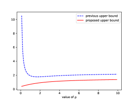
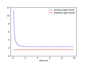
Figure 1: Left: Case 1(a), Center: Case 1(b), Right: Case 1(c)

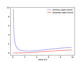
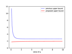
Figure 2: Left: Case 2(a), Center: Case 2(b), Right: Case 2(c)

VI Concluding remarks

We formulated and studied the problem of soft guessing under log-loss while allowing errors. We identified the optimal guessing strategy in this setting and derived single-shot upper and lower bounds on the guessing moments, expressed in terms of smooth Rényi entropies and the distortion level $D$. These bounds recover previous bounds, derived for special cases of the problem. We further derived asymptotic expansions for i.i.d. sources, leading to a sharp characterization of the guessing exponents. The results were also extended to the case where side information is available to the guesser. Finally, we established a relationship between guessing moments and the normalized cumulant generating function of codeword lengths in a corresponding variable-length source coding problem. This enabled us to bound the latter using the bounds obtained for the former.

Potential directions for future work include clarifying whether the relationship in (86), which we verified for all $D$ such that $\lfloor 2^{D}\rfloor\leq 2$, continues to hold when $\lfloor 2^{D}\rfloor>2$. The numerical results we reported above suggest that this may be the case, but currently we have no formal proof. Another direction is to refine the asymptotic analysis of the guessing moment under side information, i.e., $M^{\star}_{X^{n}|Y^{n}}(\rho,D,\epsilon)$. While we established expansions for $M^{\star}_{X^{n}}(\rho,D,\epsilon)$ up to the first- and second-order terms, for $M^{\star}_{X^{n}|Y^{n}}(\rho,D,\epsilon)$, we obtained only the first-order term. This limitation stems from the results of Sakai and Tan [14], where the smooth Rényi entropy was expanded up to the third-order term (see Lemma 9), but the conditional smooth Rényi entropy only up to the first-order term (see Lemma 10). Extending the expansion of the conditional smooth Rényi entropy, and thereby establishing the second-order term of $M^{\star}_{X^{n}|Y^{n}}(\rho,D,\epsilon)$, remains an open problem.

Appendix A Proof of Lemma 7

From the explicit formulas in Lemma 3 and Lemma 6, we can write

$$H^{\epsilon}_{\alpha}(X,Z|Y)=\inf_{(\epsilon_{y})\in\mathcal{E}_{0}(\epsilon)}\frac{\alpha}{1-\alpha}\log\left(\sum_{y\in\mathcal{Y}}P_{Y}(y)\exp\left(\frac{1-\alpha}{\alpha}H_{\alpha}^{\epsilon_{y}}\left(P_{X,Z|Y=y}\right)\right)\right),$$ (152)

where $H_{\alpha}^{\epsilon_{y}}\left(P_{X,Z|Y=y}\right)$ is the smooth Rényi entropy of $P_{X,Z|Y=y}$. From Corollary 1, we know that for every $y\in\mathcal{Y}$, we have

$$H_{\alpha}^{\epsilon_{y}}\left(P_{X,Z|Y=y}\right)\leq\tilde{H}_{\alpha}^{0}\left(P_{X|Z,Y=y}\right)+H_{\alpha}^{\epsilon_{y}}\left(P_{Z|Y=y}\right),$$ (153)

where $\tilde{H}^{0}_{\alpha}(P_{X|Z,Y=y})$ is bounded above as

$$\tilde{H}^{0}_{\alpha}(P_{X|Z,Y=y}) =\max_{z:P_{Z|Y}(z|y)>0}H_{\alpha}(P_{X|Z=z,Y=y})$$ (154)

$$\leq\max_{y:P_{Y}(y)>0}\max_{z:P_{Z|Y}(z|y)>0}H_{\alpha}(P_{X|Z=z,Y=y})$$ (155)

$$=\tilde{H}^{0}_{\alpha}(X|Z,Y).$$ (156)

Plugging everything back into (152), we get

$$H^{\epsilon}_{\alpha}(X,Z|Y) \leq\inf_{(\epsilon_{y})\in\mathcal{E}_{0}(\epsilon)}\frac{\alpha}{1-\alpha}\log\left(\sum_{y\in\mathcal{Y}}P_{Y}(y)\exp\left(\frac{1-\alpha}{\alpha}\left(\tilde{H}^{0}_{\alpha}(X|Z,Y)+H_{\alpha}^{\epsilon_{y}}\left(P_{Z|Y=y}\right)\right)\right)\right)$$ (157)

$$=\tilde{H}^{0}_{\alpha}(X|Z,Y)+\inf_{(\epsilon_{y})\in\mathcal{E}_{0}(\epsilon)}\frac{\alpha}{1-\alpha}\log\left(\sum_{y\in\mathcal{Y}}P_{Y}(y)\exp\left(\frac{1-\alpha}{\alpha}H_{\alpha}^{\epsilon_{y}}\left(P_{Z|Y=y}\right)\right)\right)$$ (158)

$$=\tilde{H}^{0}_{\alpha}(X|Z,Y)+H_{\alpha}^{\epsilon}(Z|Y),$$ (159)

which completes the proof of Lemma 7.

Appendix B Proof of Proposition 1

Consider an arbitrary $D$-admissible strategy $(\mathcal{G}_{\mathrm{soft}}(D),\pi)$ that satisfies the error probability constraint

$$P_{e}=\mathbb{P}[G(X)=0]\leq\epsilon.$$ (160)

To show Proposition 1, it suffices to prove that

$$\mathbb{E}\left[G^{\star}(X)^{\rho}\right]\leq\mathbb{E}\left[G(X)^{\rho}\right].$$ (161)

To this end, we follow in the footsteps of Sakai and Tan in their proof of [14, Lemma 10], which in turn, employs the competitive optimality idea in the proof of Arıkan [5]. In particular, to prove (161), we will show that

$$\mathbb{P}\left[G^{\star}(X)\leq k\right]\geq\mathbb{P}\left[G(X)\leq k\right]\quad(\forall k\in\{0,1,\ldots,N\}).$$ (162)

This is because if we can prove (162), then it holds that

$$\mathbb{E}\left[G^{\star}(X)^{\rho}\right] =\sum_{k=1}^{N}\big(k^{\rho}-(k-1)^{\rho}\big)\mathbb{P}\left[G^{\star}(X)\geq k\right]$$ (163)

$$\leq\sum_{k=1}^{N}\big(k^{\rho}-(k-1)^{\rho}\big)\mathbb{P}\left[G(X)\geq k\right]$$ (164)

$$=\mathbb{E}\left[G(X)^{\rho}\right].$$ (165)

We proceed by noting that for every $k=0,1,2,\ldots,K-1$, where $K$ is as defined in (49), we have

$$\mathbb{P}\left[G(X)\leq k\right] =\mathbb{P}\left[G(X)=0\right]+\sum_{i=1}^{k}\mathbb{P}\left[G(X)=i\right]$$ (166)

$$=\mathbb{P}\left[G(X)=0\right]+\sum_{i=1}^{k}\lambda_{i}\left(\sum_{x\in g^{-1}(i)}P_{X}(x)\right)$$ (167)

$$\leq\mathbb{P}\left[G^{\star}(X)=0\right]+\sum_{i=1}^{k}\lambda_{i}\left(\sum_{x\in g^{-1}(i)}P_{X}(x)\right)$$ (168)

$$\leq\mathbb{P}\left[G^{\star}(X)=0\right]+\sum_{i=1}^{k}\lambda^{\star}_{i}\left(\sum_{x\in(g^{\star})^{-1}(i)}P_{X}(x)\right)$$ (169)

$$=\mathbb{P}\left[G^{\star}(X)=0\right]+\sum_{i=1}^{k}\mathbb{P}\left[G^{\star}(X)=i\right]$$ (170)

$$=\mathbb{P}\left[G^{\star}(X)\leq k\right],$$ (171)

where (168) is due to the inequality $\mathbb{P}\left[G(X)=0\right]\leq\mathbb{P}\left[G^{\star}(X)=0\right]$ (see (63) and (160)); and (169) follows from

$$\sum_{i=1}^{k}\lambda_{i}\left(\sum_{x\in g^{-1}(i)}P_{X}(x)\right)\leq\sum_{i=1}^{k}\lambda^{\star}_{i}\left(\sum_{x\in(g^{\star})^{-1}(i)}P_{X}(x)\right).$$ (172)

To verify (172), the following lemma by Shkel and Verdú [44] is useful.

Lemma 11 ([44, Lemma 1]).

For the log-loss defined in (11), we say that $\hat{P}\in\mathcal{P}(\mathcal{X})$ $D$-covers $x\in\mathcal{X}$ if $d(x,\hat{P})\leq D$. Then, no soft reconstruction $\hat{P}$ can $D$-cover more than $\lfloor\exp(D)\rfloor$ realization of $X$, i.e., it holds that

$$\big|\big\{x\in\mathcal{X}:\hat{P}~D\text{-covers}~x\big\}\big|\leq\lfloor\exp(D)\rfloor,\ \ \text{for every}\ \hat{P}\in\mathcal{P}(\mathcal{X}).$$ (173)

Recall that in the scheme $\mathcal{G}_{\mathrm{soft}}^{\star}(D)$, each of the lists $\mathcal{L}_{1},\mathcal{L}_{2},\ldots,\mathcal{L}_{K-1}$ contains $\lfloor\exp(D)\rfloor$ realizations of $X$ (see (52)), and higher probability realizations are assigned shorter guessing orders. Combining this with Lemma 11, we get

$$\sum_{x\in g^{-1}(i)}P_{X}(x)\leq\sum_{x\in(g^{\star})^{-1}(i)}P_{X}(x)$$ (174)

for every $i=1,2,\ldots,K-1$. Moreover, from the property of $\pi^{\star}$ that $\pi^{\star}_{i}=0$ for $i=1,2,\ldots,K-1$ (see (57)), and hence $\lambda^{\star}_{i}=1$ for $i=1,2,\ldots,K-1$ (see (58)), we get

$$\lambda_{i}\leq\lambda^{\star}_{i}$$ (175)

for every $i=1,2,\ldots,K-1$. Therefore, by combining (174) and (175), we have (172).

To complete the proof, we wish to show that for every $k=K,K+1,\ldots,N$, it also holds that

$$\mathbb{P}\left[G(X)\leq k\right]\leq\mathbb{P}\left[G^{\star}(X)\leq k\right].$$ (176)

This follows by noting that

$$\mathbb{P}\left[G^{\star}(X)\leq K\right] =\mathbb{P}\left[G^{\star}(X)=0\right]+\sum_{i=1}^{K}\mathbb{P}\left[G^{\star}(X)=i\right]$$ (177)

$$=\epsilon+\sum_{i=1}^{K-1}\left(\sum_{x\in(g^{\star})^{-1}(i)}P_{X}(x)\right)+\lambda^{\star}_{K}\left(\sum_{x\in(g^{\star})^{-1}(K)}P_{X}(x)\right)$$ (178)

$$=\epsilon+\sum_{i=1}^{i^{*}_{X}}Q^{\epsilon}_{X}(i)$$ (179)

$$=\epsilon+(1-\epsilon)$$ (180)

$$=1.$$ (181)

Therefore, we have shown that (162) holds, which completes the proof.

Appendix C Proof of Proposition 2

C-A Upper Bound

As in Section III-B, let $L:=\lfloor\exp(D)\rfloor$. First, we consider the case where $L>1$. From (69), we have

$$M^{\star}_{X}(\rho,D,\epsilon) =\sum_{i=1}^{K-1}\left(\sum_{j=(i-1)L+1}^{iL}Q^{\epsilon}_{X}(j)\right)i^{\rho}+\left(\sum_{i=(K-1)L+1}^{i^{*}_{X}}Q^{\epsilon}_{X}(i)\right)K^{\rho}$$ (182)

$$=\sum_{j=1}^{i^{*}_{X}}Q^{\epsilon}_{X}(j)\left\lceil\frac{j}{L}\right\rceil^{\rho}$$ (183)

$$=\sum_{j=1}^{i^{*}_{X}}Q^{\epsilon}_{X}(j)\left\lceil\frac{1}{L}\sum_{k:k\leq j}1\right\rceil^{\rho}$$ (184)

$$\leq\sum_{j=1}^{i^{*}_{X}}Q^{\epsilon}_{X}(j)\left\lceil\frac{1}{L}\sum_{k:k\leq j}\left(\frac{Q^{\epsilon}_{X}(k)}{Q^{\epsilon}_{X}(j)}\right)^{\frac{1}{1+\rho}}\right\rceil^{\rho}$$ (185)

$$\leq\sum_{j=1}^{i^{*}_{X}}Q^{\epsilon}_{X}(j)\left\lceil\frac{1}{L}\sum_{k=1}^{i^{*}_{X}}\left(\frac{Q^{\epsilon}_{X}(k)}{Q^{\epsilon}_{X}(j)}\right)^{\frac{1}{1+\rho}}\right\rceil^{\rho}$$ (186)

$$\leq\sum_{j=1}^{i^{*}_{X}}Q^{\epsilon}_{X}(j)\left\{1+2^{\rho}\left(\frac{1}{L}\sum_{k=1}^{i^{*}_{X}}\left(\frac{Q^{\epsilon}_{X}(k)}{Q^{\epsilon}_{X}(j)}\right)^{\frac{1}{1+\rho}}\right)^{\rho}\right\}$$ (187)

$$=\sum_{j=1}^{i^{*}_{X}}Q^{\epsilon}_{X}(j)+\left(\frac{2}{L}\right)^{\rho}\left(\sum_{j=1}^{i^{*}_{X}}[Q^{\epsilon}_{X}(j)]^{\frac{1}{1+\rho}}\right)^{1+\rho}$$ (188)

$$=1-\epsilon+\left(\frac{2}{L}\right)^{\rho}\exp\left(\rho H^{\epsilon}_{\frac{1}{1+\rho}}(X)\right)$$ (189)

$$=1-\epsilon+2^{\rho}\exp\left(\rho H^{\epsilon}_{\frac{1}{1+\rho}}(X)-\rho\log\lfloor\exp(D)\rfloor\right),$$ (190)

where (185) follows from the definition of $Q^{\epsilon}_{X}$ in Lemma 3; (187) is due to the of Bunte-Lapidoth inequality $\lceil\xi\rceil^{\rho}<1+2^{\rho}\xi^{\rho}$ for $\xi\geq 0$ and $\rho>0$ (see [48, Eq. (26)]); and (189) follows from Lemma 3.

Next, we consider the case where $L=1$. Here, instead of (183), we have

$$M^{\star}_{X}(\rho,D,\epsilon)=\sum_{j=1}^{i^{*}_{X}}Q^{\epsilon}_{X}(j)j^{\rho},$$ (191)

and hence we do not need to use the inequality $\lceil\xi\rceil^{\rho}<1+2^{\rho}\xi^{\rho}$ as in the above case. Hence, we directly obtain

$$M^{\star}_{X}(\rho,D,\epsilon)\leq\exp\left(\rho H^{\epsilon}_{\frac{1}{1+\rho}}(X)\right).$$ (192)

C-B Lower Bound

We utilize the properties of the smooth Rényi entropy. Since $\rho>0$, it holds that $0<1/(1+\rho)<1$. Hence, we have

$$H^{\epsilon}_{\frac{1}{1+\rho}}(Z) \geq H^{\epsilon}_{\frac{1}{1+\rho}}(X,Z)-\tilde{H}^{0}_{\frac{1}{1+\rho}}(X|Z)$$ (193)

$$\geq H^{\epsilon}_{\frac{1}{1+\rho}}(X)-\tilde{H}^{0}_{\frac{1}{1+\rho}}(X|Z),$$ (194)

where $Z$ is defined by (47); (193) follows from the chain rule in Corollary 1; and (194) is due to monotonicity in Lemma 1. Next, we bound the term $\tilde{H}^{0}_{\frac{1}{1+\rho}}(X|Z)$ above as

$$\tilde{H}^{0}_{\frac{1}{1+\rho}}(X|Z) =\max_{z:P_{Z}(z)>0}H_{\frac{1}{1+\rho}}(P_{X|Z=z})$$ (195)

$$\leq\max_{z:P_{Z}(z)>0}\log|\mathrm{supp}(P_{X|Z=z})|.$$ (196)

Since $Z$ represents the index of the list containing $X$, as defined in (47), then the cardinality of the support of $X$ given $Z=z$ is at most $\lfloor\exp(D)\rfloor$. Hence, for every $z$ with $P_{Z}(z)>0$, we have

$$\log|\mathrm{supp}(P_{X|Z=z})|\leq\log\lfloor\exp(D)\rfloor,$$ (197)

from which it follows that

$$\tilde{H}^{0}_{\frac{1}{1+\rho}}(X|Z)\leq\log\lfloor\exp(D)\rfloor.$$ (198)

Finally, combining (46), (194), and (198), we obtain (85).

Appendix D Proof of Proposition 5

D-A Upper Bound

By the same argument used in the upper bound proof for Proposition 2, for any given side information realization $y$, $M_{X|Y=y}^{\star}(\rho,D,\epsilon_{y})$ on the right-hand side of (118) is upper bounded as

$$M_{X|Y=y}^{\star}(\rho,D,\epsilon_{y})\leq 1-\epsilon_{y}+\left(\frac{2}{L}\right)^{\rho}\left(\sum_{j=1}^{i_{X|y}^{*}}[Q^{\epsilon_{y}}_{X|Y}(x^{j}_{y}|y)]^{\frac{1}{1+\rho}}\right)^{1+\rho}.$$ (199)

Next, we take the expectation with respect to $Y$ and then the infimum over $(\epsilon_{y})\in\mathcal{E}_{0}(\epsilon)$. From the explicit form of Kuzuoka’s conditional smooth Rényi entropy in Lemma 6, we obtain (126). The upper bound for $0\leq D<1$ is similarly proved.

D-B Lower Bound

From the conditional chain rule in Lemma 7 and the conditional monotonicity in Lemma 5, we obtain

$$H^{\epsilon}_{\frac{1}{1+\rho}}(Z|Y) \geq H^{\epsilon}_{\frac{1}{1+\rho}}(X,Z|Y)-\tilde{H}^{0}_{\frac{1}{1+\rho}}(X|Z,Y)$$ (200)

$$\geq H^{\epsilon}_{\frac{1}{1+\rho}}(X|Y)-\tilde{H}^{0}_{\frac{1}{1+\rho}}(X|Z,Y).$$ (201)

Using similar argument to the ones used in the lower bound proof for Proposition 2, the term $\tilde{H}^{0}_{\frac{1}{1+\rho}}(X|Z,Y)$ is bounded as

$$\tilde{H}^{0}_{\frac{1}{1+\rho}}(X|Z,Y) =\max_{y:P_{Y}(y)>0}\max_{z:P_{Z|Y}(z|y)>0}H_{\alpha}(P_{X|Z=z,Y=y})$$ (202)

$$\leq\max_{y:P_{Y}(y)>0}\max_{z:P_{Z|Y}(z|y)>0}\log|\mathrm{supp}(P_{X|Z=z,Y=y})|$$ (203)

$$\leq\log\lfloor\exp(D)\rfloor.$$ (204)

Finally, combining (117), (201), and (204), we obtain (127).

Appendix E Proof of Theorem 3

Here we prove (141), (142) and (143). We begin by finding an optimal variable-length source code that attains $\Lambda_{X}^{\star}(\rho,D,\epsilon)$ in (139). We denote this by $(f^{\star}_{X},\varphi^{\star}_{X})$. Note that in [44, Section IV], Shkel and Verdú found a competitively optimal variable-length source code under log-loss with no errors. The code we present next can be seen as an extension of their code.

Let $L:=\lfloor\exp(D)\rfloor$. For $l=1,2,\ldots,\left\lceil\frac{|\mathcal{X}|}{L}\right\rceil-1$, define the following sets (or lists)

$$\mathcal{L}_{l}:=\{(l-1)L+1,(l-1)L+2,\ldots,lL\}$$ (205)

and

$$\mathcal{L}_{\left\lceil\frac{|\mathcal{X}|}{L}\right\rceil}:=\left\{\left(\left\lceil\frac{|\mathcal{X}|}{L}\right\rceil-1\right)L+1,\ldots,|\mathcal{X}|\right\}.$$ (206)

Let $\mathcal{L}_{l^{*}}\in\left\{\mathcal{L}_{1},\mathcal{L}_{2},\ldots,\mathcal{L}_{\left\lceil\frac{|\mathcal{X}|}{L}\right\rceil}\right\}$ be the set such that $i^{*}_{X}\in\mathcal{L}_{l^{*}}$, where $i^{*}_{X}$ is defined in (23). The encoder $f^{*}_{X}$ maps the elements in $\mathcal{L}_{1},\mathcal{L}_{2},\ldots,\mathcal{L}_{l^{*}-1}$ to the elements of $\{0,1\}^{*}$ in the lexicographic order, i.e.,

$$f^{\star}_{X}(x)=\begin{cases}\varnothing,&x\in\mathcal{L}_{1},\\ 0,&x\in\mathcal{L}_{2},\\ 1,&x\in\mathcal{L}_{3},\\ 00,&x\in\mathcal{L}_{4},\\ 01,&x\in\mathcal{L}_{5},\\ 10,&x\in\mathcal{L}_{6},\\ 11,&x\in\mathcal{L}_{7},\\ 000,&x\in\mathcal{L}_{8},\\ &\vdots\\ {\sf s},&x\in\mathcal{L}_{l^{*}-1},\end{cases}$$ (207)

where ${\sf s}\in\{0,1\}^{*}$ is a binary string of length $\lfloor\log(l^{*}-1)\rfloor$. Second, $f^{\star}_{X}$ maps each element $x\in\mathcal{L}_{l^{*}}$ as

$$f^{\star}_{X}(x)=\begin{cases}\varnothing,&\mathrm{with~probability}~\alpha,\\ {\sf s}^{+},&\mathrm{with~probability}~1-\alpha,\end{cases}$$ (208)

where ${\sf s}^{+}\in\{0,1\}^{*}$ is a binary string that follows ${\sf s}$ in the lexicographic order, and $\alpha$ is chosen so that

$$\epsilon=\alpha\sum_{x\in\mathcal{L}_{l^{*}}}P_{X}(x)+\sum_{i=l^{*}+1}^{\left\lceil\frac{|\mathcal{X}|}{L}\right\rceil}\sum_{x\in\mathcal{L}_{i}}P_{X}(x).$$ (209)

Finally, $f^{\star}_{X}$ maps all the elements in $\mathcal{L}_{l^{*}+1},\mathcal{L}_{l^{*}+2},\ldots,\mathcal{L}_{\left\lceil\frac{|\mathcal{X}|}{L}\right\rceil}$ to the empty string $\varnothing$. The decoder $\varphi^{\star}_{X}$ is defined as

$$\varphi^{\star}_{X}(s)=\begin{cases}\hat{P}_{1},&s=\varnothing,\\ \hat{P}_{2},&s=0,\\ \hat{P}_{3},&s=1,\\ \hat{P}_{4},&s=00,\\ &\vdots\\ \hat{P}_{l^{*}-1},&s={\sf s},\\ \hat{P}_{l^{*}},&s={\sf s}^{+},\end{cases}$$ (210)

where

$$\hat{P}_{i}(x):=\begin{cases}\frac{1}{|\mathcal{L}_{i}|},&\forall x\in\mathcal{L}_{i},\\ 0,&\mathrm{otherwise}.\end{cases}$$ (211)

From the code construction, it can be verified that excess distortion probability satisfies

$$\mathbb{P}[d(X,\varphi^{\star}_{X}(f^{\star}_{X}(X)))>D]=\epsilon,$$ (212)

and thus $(f^{\star}_{X},\varphi^{\star}_{X})$ is a $(\Lambda,D,\rho,\epsilon)$-code for some $\Lambda$. We see that $(f^{\star}_{X},\varphi^{\star}_{X})$ is optimal because no codeword can $D$-cover more than $L=\lfloor\exp(D)\rfloor$ elements in $\mathcal{X}$ (see Lemma 11), and $f^{\star}_{X}$ assigns shorter strings to the more likely elements. Therefore

$$\Lambda_{X}^{\star}(\rho,D,\epsilon)=\frac{1}{\rho}\log\mathbb{E}[\exp\{\rho\ell(f^{\star}_{X}(X))\}].$$ (213)

Next, to prove (141), we look at $\Lambda_{Z}^{\star}(\rho,0,\epsilon)$, where $Z$ is defined in (47). We repeat its definition here for convenience.

$$Z:=\left\lceil\frac{X}{\lfloor\exp(D)\rfloor}\right\rceil.$$ (214)

For coding $Z$, we have $D=0$ and the condition $\mathbb{P}[d(Z,\varphi(f(Z)))>D]\leq\epsilon$ becomes

$$\mathbb{P}[Z~\text{is correctly recovered}]\geq 1-\epsilon,$$ (215)

because $d(z,\hat{P})=0$ if and only if $\hat{P}(z)=1$, i.e., $\hat{P}$ is a correct “hard” reconstruction. An optimal code that attains $\Lambda_{Z}^{\star}(\rho,0,\epsilon)$, denoted by $(f^{\star}_{Z},\varphi^{\star}_{Z})$, is obtained by setting the encoder as $f^{\star}_{Z}(z)=f^{\star}_{X}((z-1)L+1)$ and the decoder as

$$\varphi^{\star}_{Z}(s)=\begin{cases}\hat{P}_{1},&s=\varnothing,\\ \hat{P}_{2},&s=0,\\ \hat{P}_{3},&s=1,\\ \hat{P}_{4},&s=00,\\ &\vdots\\ \hat{P}_{l^{*}-1},&s={\sf s},\\ \hat{P}_{l^{*}},&s={\sf s}^{+},\end{cases}$$ (216)

where

$$\hat{P}_{i}(z):=\begin{cases}1,&z=i,\\ 0,&\mathrm{otherwise}.\end{cases}$$ (217)

From the choice of the encoder $f^{\star}_{Z}$ and (209), it immediately follows that

$$\epsilon=\alpha P_{Z}(l^{*})+\sum_{i=l^{*}+1}^{\left\lceil\frac{|\mathcal{X}|}{L}\right\rceil}P_{Z}(i).$$ (218)

The code $(f^{\star}_{Z},\varphi^{\star}_{Z})$ coincides with the optimal code of Kostina et al. in [49, Section II]. Moreover, $Z$ corresponds to the index of the lists in (205), which explains the close relationship between $(f^{\star}_{X},\varphi^{\star}_{X})$ and $(f^{\star}_{Z},\varphi^{\star}_{Z})$. It follows that (141) is obtained as

$$\Lambda_{X}^{\star}(\rho,D,\epsilon) =\frac{1}{\rho}\log\mathbb{E}[\exp\{\rho\ell(f^{\star}_{X}(X))\}]$$ (219)

$$=\frac{1}{\rho}\log\mathbb{E}[\exp\{\rho\ell(f^{\star}_{Z}(Z))\}]=\Lambda_{Z}^{\star}(\rho,0,\epsilon).$$ (220)

Next, we prove (142). For $D=0$, the guessing problem reduces to the lossless problem of Kuzuoka [13]. Sakai and Tan [14] investigated the optimal guessing strategy for this setting, which is a special case of the lossy setting we consider. Let $G^{\star}_{Z}$ be the guessing function of the optimal guessing strategy for $Z$ with $D=0$. From [14, Lemma 10], $G^{\star}_{Z}$ is given by

$$G^{\star}_{Z}(i) =i,\quad(i=1,2,\ldots,l^{*}-1),$$ (221)

$$G^{\star}_{Z}(l^{*}) =\begin{cases}0,&\mathrm{with~probability}~\alpha,\\ l^{*},&\mathrm{with~probability}~1-\alpha,\end{cases}$$ (222)

$$G^{\star}_{Z}(j) =0,\quad\left(j=l^{*}+1,\ldots,\left\lceil\frac{|\mathcal{X}|}{L}\right\rceil\right),$$ (223)

where $\alpha$ is chosen so that (218) holds. Noting that $l^{*}=i_{Z}^{*}$, we have

$$M_{Z}^{\star}(\rho,0,\epsilon) =\mathbb{E}[G^{\star}_{Z}(Z)^{\rho}]$$ (224)

$$=\sum_{i=1}^{i_{Z}^{*}}Q^{\epsilon}_{Z}(i)i^{\rho}.$$ (225)

Combining (70) and (225), we obtain (142).

Finally, we prove (143). From the definitions of the foregoing $f^{\star}_{Z}$ and $G^{\star}_{Z}$, it holds that

$$\Lambda_{Z}^{\star}(\rho,0,\epsilon) =\frac{1}{\rho}\log\mathbb{E}[\exp(\rho\ell(f^{\star}_{Z}(Z)))]$$ (226)

$$=\frac{1}{\rho}\log\left(\sum_{z=1}^{l^{*}-1}P_{Z}(z)\exp(\rho\ell(f^{\star}_{Z}(z)))+(1-\alpha)P_{Z}(l^{*})\exp(\rho\ell({\sf s}^{+}))+\alpha P_{Z}(l^{*})\exp(\rho\ell(\varnothing))\right.$$

$$\qquad\qquad\qquad\left.+\sum_{z=l^{*}+1}^{\left\lceil\frac{|\mathcal{X}|}{L}\right\rceil}P_{Z}(z)\exp(\rho\ell(\varnothing))\right)$$ (227)

$$=\frac{1}{\rho}\log\left(\sum_{z=1}^{l^{*}-1}P_{Z}(z)\exp(\rho\ell(f^{\star}_{Z}(z)))+(1-\alpha)P_{Z}(l^{*})\exp(\rho\ell({\sf s}^{+}))+\alpha P_{Z}(l^{*})+\sum_{z=l^{*}+1}^{\left\lceil\frac{|\mathcal{X}|}{L}\right\rceil}P_{Z}(z)\right)$$ (228)

$$=\frac{1}{\rho}\log\left(\sum_{z=1}^{l^{*}-1}P_{Z}(z)\exp(\rho\ell(f^{\star}_{Z}(z)))+(1-\alpha)P_{Z}(l^{*})\exp(\rho\ell({\sf s}^{+}))+\epsilon\right)$$ (229)

$$=\frac{1}{\rho}\log\left(\sum_{z=1}^{l^{*}-1}P_{Z}(z)\exp(\rho\lfloor\log G^{\star}_{Z}(z)\rfloor)+(1-\alpha)P_{Z}(l^{*})\exp(\rho\lfloor\log l^{*}\rfloor)+\epsilon\right)$$ (230)

$$\leq\frac{1}{\rho}\log\left(\sum_{z=1}^{l^{*}-1}P_{Z}(z)\exp(\rho\log G^{\star}_{Z}(z))+(1-\alpha)P_{Z}(l^{*})\exp(\rho\log l^{*})+\epsilon\right)$$ (231)

$$=\frac{1}{\rho}\log\left(\sum_{z=1}^{l^{*}-1}P_{Z}(z)G^{\star}_{Z}(z)^{\rho}+(1-\alpha)P_{Z}(l^{*})(l^{*})^{\rho}+\epsilon\right)$$ (232)

$$=\frac{1}{\rho}\log\left(\mathbb{E}[G^{\star}_{Z}(Z)^{\rho}]+\epsilon\right)$$ (233)

$$=\frac{1}{\rho}\log\left(M_{Z}^{\star}(\rho,0,\epsilon)+\epsilon\right),$$ (234)

where (228) is due to $\ell(\varnothing)=0$; (229) follows from (218); (230) follows because $\ell(f^{\star}_{Z}(z))=\lfloor\log G^{\star}_{Z}(z)\rfloor$ for $z=1,\ldots,l^{*}-1$ and $\ell({\sf s}^{+})=\lfloor\log l^{*}\rfloor$ from the definitions of $f^{\star}_{Z}$ and $G^{\star}_{Z}$; and (231) is due to $\lfloor a\rfloor\leq a$ for $a\in\mathbb{R}$. Moreover, we have

$$\Lambda_{Z}^{\star}(\rho,0,\epsilon) >\frac{1}{\rho}\log\left(\sum_{z=1}^{l^{*}-1}P_{Z}(z)\exp(\rho\log G^{\star}_{Z}(z)-\rho)+(1-\alpha)P_{Z}(l^{*})\exp(\rho\log l^{*}-\rho)+\epsilon\right)$$ (235)

$$=\frac{1}{\rho}\log\left(2^{-\rho}\left[\sum_{z=1}^{l^{*}-1}P_{Z}(z)G^{\star}_{Z}(z)^{\rho}+(1-\alpha)P_{Z}(l^{*})(l^{*})^{\rho}\right]+\epsilon\right)$$ (236)

$$=\frac{1}{\rho}\log\left(2^{-\rho}\mathbb{E}[G^{\star}_{Z}(Z)^{\rho}]+\epsilon\right)=\frac{1}{\rho}\log\left(2^{-\rho}M_{Z}^{\star}(\rho,0,\epsilon)+\epsilon\right),$$ (237)

where (235) follows from (230) and $\lfloor a\rfloor>a-1$ for $a\in\mathbb{R}$.

References

- [1] S. Saito, “Soft guessing under log-loss distortion allowing errors,” in 2024 IEEE International Symposium on Information Theory (ISIT), 2024, pp. 2957–2962.
- [2] ——, “An upper bound of cumulant generating function of codeword lengths in variable-length lossy source coding under logarithmic loss,” in 2024 International Symposium on Information Theory and its Applications (ISITA), 2024, pp. 346–348.
- [3] S. Saito and H. Joudeh, “A note on two upper bounds of cumulant generating function of codeword lengths in variable-length lossy source coding under logarithmic loss,” in the 47th Symposium on Information Theory and its Applications, 2024, (a domestic conference in Japan).
- [4] J. Massey, “Guessing and entropy,” in 1994 IEEE International Symposium on Information Theory (ISIT), 1994, pp. 204–.
- [5] E. Arıkan, “An inequality on guessing and its application to sequential decoding,” IEEE Transactions on Information Theory, vol. 42, no. 1, pp. 99–105, 1996.
- [6] A. Rényi, “On measures of entropy and information,” in Proceedings of the Fourth Berkeley Symposium on Mathematical Statistics and Probability, 1961, pp. 547–561.
- [7] S. Arimoto, “Information measures and capacity of order for discrete memoryless channels,” Topics in Information Theory, pp. 41–52, 1977.
- [8] E. Arıkan and N. Merhav, “Guessing subject to distortion,” IEEE Transactions on Information Theory, vol. 44, no. 3, pp. 1041–1056, 1998.
- [9] A. Cohen and N. Merhav, “Universal randomized guessing subject to distortion,” IEEE Transactions on Information Theory, vol. 68, no. 12, pp. 7714–7734, 2022.
- [10] N. Merhav, R. Roth, and E. Arıkan, “Hierarchical guessing with a fidelity criterion,” IEEE Transactions on Information Theory, vol. 45, no. 1, pp. 330–337, 1999.
- [11] S. Saito and T. Matsushima, “Non-asymptotic fundamental limits of guessing subject to distortion,” in 2019 IEEE International Symposium on Information Theory (ISIT), 2019, pp. 652–656.
- [12] H. Wu and H. Joudeh, “Soft guessing under logarithmic loss,” in 2023 IEEE International Symposium on Information Theory (ISIT), 2023, pp. 466–471.
- [13] S. Kuzuoka, “On the conditional smooth rényi entropy and its applications in guessing and source coding,” IEEE Transactions on Information Theory, vol. 66, no. 3, pp. 1674–1690, 2020.
- [14] Y. Sakai and V. Y. F. Tan, “On smooth rényi entropies: A novel information measure, one-shot coding theorems, and asymptotic expansions,” IEEE Transactions on Information Theory, vol. 68, no. 3, pp. 1496–1531, 2022.
- [15] R. Sundaresan, “Guessing under source uncertainty,” IEEE Transactions on Information Theory, vol. 53, no. 1, pp. 269–287, 2007.
- [16] E. Arıkan, “Large deviations of probability rank,” in 2000 IEEE International Symposium on Information Theory (ISIT), 2000, p. 27.
- [17] M. M. Christiansen and K. R. Duffy, “Guesswork, large deviations, and shannon entropy,” IEEE Transactions on Information Theory, vol. 59, no. 2, pp. 796–802, 2013.
- [18] M. K. Hanawal and R. Sundaresan, “Guessing revisited: A large deviations approach,” IEEE Transactions on Information Theory, vol. 57, no. 1, pp. 70–78, 2011.
- [19] C. Pfister and W. Sullivan, “Rényi entropy, guesswork moments, and large deviations,” IEEE Transactions on Information Theory, vol. 50, no. 11, pp. 2794–2800, 2004.
- [20] R. Sundaresan, “Guessing based on length functions,” in 2007 IEEE International Symposium on Information Theory (ISIT), 2007, pp. 716–719.
- [21] E. Arıkan and N. Merhav, “Joint source-channel coding and guessing with application to sequential decoding,” IEEE Transactions on Information Theory, vol. 44, no. 5, pp. 1756–1769, 1998.
- [22] A. Burin and O. Shayevitz, “Reducing guesswork via an unreliable oracle,” IEEE Transactions on Information Theory, vol. 64, no. 11, pp. 6941–6953, 2018.
- [23] W. Huleihel, S. Salamatian, and M. Médard, “Guessing with limited memory,” in 2017 IEEE International Symposium on Information Theory (ISIT), 2017, pp. 2253–2257.
- [24] D. Malone and W. Sullivan, “Guesswork and entropy,” IEEE Transactions on Information Theory, vol. 50, no. 3, pp. 525–526, 2004.
- [25] S. Salamatian, A. Beirami, A. Cohen, and M. Médard, “Centralized vs decentralized multi-agent guesswork,” in 2017 IEEE International Symposium on Information Theory (ISIT), 2017, pp. 2258–2262.
- [26] S. Salamatian, W. Huleihel, A. Beirami, A. Cohen, and M. Médard, “Why botnets work: Distributed brute-force attacks need no synchronization,” IEEE Transactions on Information Forensics and Security, vol. 14, no. 9, pp. 2288–2299, 2019.
- [27] Y. Yona and S. Diggavi, “The effect of bias on the guesswork of hash functions,” in 2017 IEEE International Symposium on Information Theory (ISIT), 2017, pp. 2248–2252.
- [28] M. M. Christiansen, K. R. Duffy, F. du Pin Calmon, and M. Médard, “Multi-user guesswork and brute force security,” IEEE Transactions on Information Theory, vol. 61, no. 12, pp. 6876–6886, 2015.
- [29] A. Beirami, R. Calderbank, K. Duffy, and M. Médard, “Quantifying computational security subject to source constraints, guesswork and inscrutability,” in 2015 IEEE International Symposium on Information Theory (ISIT), 2015, pp. 2757–2761.
- [30] N. Merhav and A. Cohen, “Universal randomized guessing with application to asynchronous decentralized brute–force attacks,” IEEE Transactions on Information Theory, vol. 66, no. 1, pp. 114–129, 2020.
- [31] R. Graczyk, A. Lapidoth, N. Merhav, and C. Pfister, “Guessing based on compressed side information,” IEEE Transactions on Information Theory, vol. 68, no. 7, pp. 4244–4256, 2022.
- [32] N. Merhav, “Guessing individual sequences: Generating randomized guesses using finite–state machines,” IEEE Transactions on Information Theory, vol. 66, no. 5, pp. 2912–2920, 2020.
- [33] ——, “Noisy guesses,” IEEE Transactions on Information Theory, vol. 66, no. 8, pp. 4796–4803, 2020.
- [34] G. R. Kurri, O. Kosut, and L. Sankar, “Evaluating multiple guesses by an adversary via a tunable loss function,” in 2021 IEEE International Symposium on Information Theory (ISIT), 2021, pp. 2002–2007.
- [35] I. Sason and S. Verdú, “Improved bounds on lossless source coding and guessing moments via rényi measures,” IEEE Transactions on Information Theory, vol. 64, no. 6, pp. 4323–4346, 2018.
- [36] I. Sason, “Tight bounds on the rényi entropy via majorization with applications to guessing and compression,” Entropy, vol. 20, no. 12, 2018.
- [37] K. R. Duffy, J. Li, and M. Médard, “Capacity-achieving guessing random additive noise decoding,” IEEE Transactions on Information Theory, vol. 65, no. 7, pp. 4023–4040, 2019.
- [38] K. R. Duffy, W. An, and M. Médard, “Ordered reliability bits guessing random additive noise decoding,” IEEE Transactions on Signal Processing, vol. 70, pp. 4528–4542, 2022.
- [39] H. Joudeh, “On guessing random additive noise decoding,” in 2024 IEEE International Symposium on Information Theory (ISIT), 2024, pp. 1291–1296.
- [40] V. Y. F. Tan and H. Joudeh, “Ensemble-tight second-order asymptotics and exponents for guessing-based decoding with abandonment,” IEEE Transactions on Information Theory, vol. 71, no. 10, pp. 7555–7567, 2025.
- [41] R. Renner and S. Wolf, “Simple and tight bounds for information reconciliation and privacy amplification,” in Advances in Cryptology - ASIACRYPT 2005, B. Roy, Ed. Berlin, Heidelberg: Springer Berlin Heidelberg, 2005, pp. 199–216.
- [42] T. A. Courtade and R. D. Wesel, “Multiterminal source coding with an entropy-based distortion measure,” in 2011 IEEE International Symposium on Information Theory (ISIT), 2011, pp. 2040–2044.
- [43] T. A. Courtade and T. Weissman, “Multiterminal source coding under logarithmic loss,” IEEE Transactions on Information Theory, vol. 60, no. 1, pp. 740–761, 2014.
- [44] Y. Y. Shkel and S. Verdú, “A single-shot approach to lossy source coding under logarithmic loss,” IEEE Transactions on Information Theory, vol. 64, no. 1, pp. 129–147, 2018.
- [45] S. Fehr and S. Berens, “On the conditional rényi entropy,” IEEE Transactions on Information Theory, vol. 60, no. 11, pp. 6801–6810, 2014.
- [46] T. M. Cover and J. A. Thomas, Elements of Information Theory, 2nd ed. John Wiley & Sons, 2006.
- [47] H. Koga, “Characterization of the smooth rényi entropy using majorization,” in 2013 IEEE Information Theory Workshop (ITW), 2013, pp. 1–5.
- [48] C. Bunte and A. Lapidoth, “Encoding tasks and rényi entropy,” IEEE Transactions on Information Theory, vol. 60, no. 9, pp. 5065–5076, 2014.
- [49] V. Kostina, Y. Polyanskiy, and S. Verdú, “Variable-length compression allowing errors,” IEEE Transactions on Information Theory, vol. 61, no. 8, pp. 4316–4330, 2015.
- [50] L. L. Campbell, “A coding theorem and rényi’s entropy,” Inf. Control., vol. 8, pp. 423–429, 1965.
- [51] T. A. Courtade and S. Verdú, “Cumulant generating function of codeword lengths in optimal lossless compression,” in 2014 IEEE International Symposium on Information Theory (ISIT), 2014, pp. 2494–2498.
- [52] I. Kontoyiannis and S. Verdú, “Optimal lossless data compression: Non-asymptotics and asymptotics,” IEEE Transactions on Information Theory, vol. 60, no. 2, pp. 777–795, 2014.
- [53] T. A. Courtade and S. Verdú, “Variable-length lossy compression and channel coding: Non-asymptotic converses via cumulant generating functions,” in 2014 IEEE International Symposium on Information Theory (ISIT), 2014, pp. 2499–2503.
- [54] S. Saito and T. Matsushima, “Non-asymptotic bounds of cumulant generating function of codeword lengths in variable-length lossy compression,” IEEE Transactions on Information Theory, vol. 69, no. 4, pp. 2113–2119, 2023.