TripScore: Benchmarking and rewarding real-world travel planning with fine-grained evaluation

Abstract

Travel planning is a valuable yet complex task that poses significant challenges even for advanced large language models (LLMs). While recent benchmarks have advanced in evaluating LLMs’ planning capabilities, they often fall short in evaluating feasibility, reliability, and engagement of travel plans. We introduce a comprehensive benchmark for travel planning that unifies fine-grained criteria into a single reward, enabling direct comparison of plan quality and seamless integration with reinforcement learning (RL). Our evaluator achieves moderate agreement with travel-expert annotations (60.75%) and outperforms multiple LLM-as-judge baselines. We further release a large-scale dataset of 4,870 queries including 219 real-world, free-form requests for generalization to authentic user intent. Using this benchmark, we conduct extensive experiments across diverse methods and LLMs, including test-time computation, neuro-symbolic approaches, supervised fine-tuning, and RL via GRPO. Across base models, RL generally improves itinerary feasibility over prompt-only and supervised baselines, yielding higher unified reward scores.

1 Introduction

Planning is widely regarded as one of the most sophisticated cognitive skills in humans. Recently, large language models (LLMs) (Anil et al., 2023; OpenAI, 2023) have demonstrated promising capabilities in complex reasoning tasks. However, benchmarks such as meeting scheduling and graph coloring (Jimenez et al., 2024; Zheng et al., 2024; Stechly et al., 2025) reveal that planning remains a challenging domain to solve comprehensively.

Travel planning, in particular, has gained significant attention due to its real-world applicability and inherent complexity (Shao et al., 2024a; Chen et al., 2024). Several benchmarks have been proposed to evaluate AI systems’ travel planning capabilities. TravelPlanner (Xie et al., 2024) revealed that even state-of-the-art models achieved only a 4.4% pass rate when evaluating LLMs solely on their planning skills.  Hao et al. (2025) later proposed a method integrating LLM-based and algorithm-based planning approaches, dramatically improving the pass rate to 97%. Recognizing the limitations of TravelPlanner’s simplicity, more sophisticated benchmarks such as ChinaTravel (Shao et al., 2024a) and TripTailor (Wang et al., 2025) were developed. These benchmarks incorporate larger datasets, user preferences, and soft constraints to better reflect real-world scenarios. However, user queries in these benchmarks are primarily based on LLM-generated content or questionnaires, which may not fully capture the nuances and unpredictability of real-world travel requests. For instance, a user might need to plan around a concert, prefer a themed trail (e.g., a Harry Potter or Hans Christian Andersen route), or prioritize certain landmarks.

To address the travel planning problem, various approaches have been proposed to enhance the planning capabilities of LLMs. Shao et al. (2024a) propose utilizing LLMs to determine the next step while employing depth-first search to identify the optimal plan. Kambhampati et al. (2024) advocate for iterative thinking based on feedback. Gui et al. (2025) introduce the construction of hypertree-structured planning outlines to guide models in hierarchical thinking. While these methods have shown promise in passing constraints, they rely heavily on test-time computation, which may not be practical in real-world applications where users eagerly await immediate results. They also continue to suffer from hallucinations, misaligned schedules, and unengaging itineraries, highlighting the need for reliable fine-grained metrics and a robust unified reward, which can be leveraged in reinforcement learning for better alignment. Recently, reinforcement learning (DeepSeek-AI et al., 2025; Hao et al., 2023) (RL) has emerged as a key paradigm for scaling LLM reasoning capability and shows strong potential for planning. The lack of high-quality user query dataset with fine-grained unified assessments further hinders the development of more advanced travel planning methods.

In this work, we propose a comprehensive framework that evaluates itinerary quality along fine-grained criteria and aggregates the results into a single reward score. Leveraging this reward, our benchmark enables the integration with RL, and our experiments accordingly assess the resulting improvements in effectiveness and performance. Our main contributions are:

• Comprehensive Evaluation Framework. We propose a comprehensive evaluation framework that synthesizes multiple criteria into a single reward for trip quality assessment, enabling more direct comparisons of plan quality. Our evaluation shows moderate agreement with travel-expert annotations (60.75%), and it outperforms a range of LLM-as-judge baselines.

• Large-scale Dataset. We introduce a 4,870 query dataset, split into 3,493 training, 158 validation, and 1,219 test samples. The test set includes 1,000 synthetic queries and 219 real-world, free-form user requests, enabling a fair assessment of generalization to authentic requests.

• Experimental Analysis. We conduct extensive experiments across diverse methods and LLMs on our benchmark, including test-time computation, neuro-symbolic approaches, and fine-tuning. Across base models, reinforcement learning (GRPO) generally improves itinerary quality over prompt-only and supervised baselines, resulting in higher reward scores.

Table 1: Comparison among TripScore and other travel planning benchmarks. - denotes that the corresponding dataset is not available or not provided in the original benchmark. # City Size denotes the total number of unique cities included across all data in each benchmark.

Benchmark	# Train & Dev	# Test	# City	User	Commonsense	Soft	User Preference	Unified
	Examples	Examples	Size	Request	Constraint	Constraint	Constraint	Score
TravelPlanner (Xie et al., 2024)	225	1,000	312	Synthetic	✓	✗	✗	✗
Trip Planning (Zheng et al., 2024)	-	1,600	48	Synthetic	✓	✗	✗	✗
ChinaTravel (Shao et al., 2024a)	154	1,000	10	Survey-based	✓	✓	✗	✗
TripTailor (Wang et al., 2025)	3,145	703	40	AI-generated	✓	✗	✓	✗
PersonalTravel (Shao et al., 2025)	155	1,000	77	AI-generated	✓	✗	✓	✗
TripScore (ours)	3,651	1,219	897	Real-world	✓	✓	✓	✓

2 Related Work

Travel planning methods. Researchers have developed diverse approaches to address travel planning challenges. These include solver-based optimization methods Ju et al. (2024); Hao et al. (2025) and test-time compute methods Gui et al. (2025); Shao et al. (2024a); Kambhampati et al. (2024); Yang et al. (2025b). While solver-based methods achieve high success rates by adhering to rule-based constraints, they often struggle to capture nuanced user preferences. Conversely, test-time compute methods, although potentially more flexible, face limitations in real-time deployment due to their test time demands. The key to advancing travel planning while maintaining user-friendly response times lies in enhancing the reasoning capabilities of Large Language Models (LLMs). Recently, Reinforcement Learning (RL) has emerged as a promising paradigm for improving LLMs’ reasoning and planning abilities (Hao et al., 2023; Shao et al., 2024b; DeepSeek-AI et al., 2025). Building on these advancements, our work investigates the integration of RL techniques into travel planning framework, aiming to strike an optimal balance between itinerary quality and computational efficiency.

Travel planning benchmarks. Although LLMs have made significant strides in reasoning and planning capabilities, evaluation benchmarks remain far from perfect. Previous benchmarks primarily focused on domains with clear, easily quantifiable objectives, such as mathematics (Cobbe et al., 2021; Chen et al., 2023), coding and software engineering (Nguyen et al., 2025; Jain et al., 2025), web interactions (Rawles et al., 2023; Pan et al., 2024) and games (Hu et al., 2025; Paglieri et al., 2025). Recently, several travel planning benchmarks have been proposed to assess the itinerary quality. TravelPlanner (Xie et al., 2024) introduces commonsense and hard constraints to evaluate the feasibility of itineraries. ChinaTravel (Shao et al., 2024a) and ITINERA (Tang et al., 2024) incorporate the soft constraint to evaluate the aspects that cannot be addressed as boolean constraint satisfaction problems. TripTailor (Wang et al., 2025) and RealTravel (Shao et al., 2025) further advances the field by integrating LLM-based evaluation to assess the rationality and personalization of travel itineraries. Our work introduces a comprehensive benchmark that unifies multifaceted evaluation criteria into a single reward, enabling more direct comparisons of plan quality. Furthermore, we incorporate real-world large-scale user queries to assess the model’s planning capabilities in complex and unpredictable scenarios. Table 1 provides an overview of the constraints and datasets used across the benchmarks.

3 Benchmark

3.1 Overview

We introduce TripScore, a comprehensive benchmark for evaluating LLMs’ capabilities in complex, multi-constraint travel planning scenarios. To focus on assessing the model’s core reasoning abilities, we streamline the evaluation process by directly providing all relevant information, thus eliminating extraneous tool usage complexities. This approach aligns with the sole-planning setting described in Xie et al. (2024). A representative example is illustrated in Figure 1.

Figure 1: Overview of TripScore. Given a query and the relevant recalled information, planning model is expected to deliver a plan that satisfies all specified constraints. The resulting plan is then evaluated to produce a comprehensive final reward score, reflecting its overall quality and adherence to user requirements.

Our benchmark encompasses a total of 4,870 queries, categorized into 3 splits: 3,493 training samples, 158 validation samples and 1,219 test samples. The test set contains 1,219 queries from two sources: 1,000 synthetic queries constructed from usage statistics (combinations of popular destinations and frequent durations, with randomized preferences) and 219 real-world free-form user requests. The dataset spans 897 cities, 9,376 hotels and 10,997 attractions. For a comprehensive breakdown of the dataset distribution, please refer to Appendix B.

3.2 Constraint Introduction

Table 2: Constraint description. The format constraints assess whether the plan adheres to the specified format guidelines. The commonsense constraints evaluate the logical feasibility of the plan. The soft and preference constraints measure the alignment of the plan with plan quality standards and user preferences.

Constraint	Description	Evaluation
[gray]0.85      Format Constraint
Response Format	All responses must follow the requested structure and organization exactly as specified.	Rule
Information Verification	All attractions, transportation, and hotels in the plan must come from the provided information, otherwise, it will be considered a hallucination.	Rule
Information Accuracy	Details like name and departure time must match the provided information.	Rule
Information Relevance	All descriptions must specifically match their intended attractions (e.g., not mixing up or blending details from different places).	Rule
[gray]0.85      Commonsense Constraint
Information Completeness	All necessary information must be included, especially accommodation for each destination with multi-day stay and essential transportation.	Rule
Chronological Order	All activities must be listed in chronological order.	Rule
Location Consistency	Each day’s activity must be scheduled in the city where the traveler is actually present and change only after any required transportation.	Rule
Operating Hours	Visits to attractions must only be scheduled during their confirmed opening hours.	Rule
Travel Block-Out	No activities can be scheduled between departure and arrival times during transportation.	Rule
Transport. Consistency	Arrange the transportation from the starting city to each destination in sequence to avoid jumps or repetitive routes.	Rule
[gray]0.85      Soft Constraint
Schedule Density	Each day’s itinerary should be thoughtfully paced, ensuring neither overly lengthy nor excessively brief periods of activity.	Rule
Hotel Consistency	When staying in the same city, the same hotel should be used throughout to avoid unnecessary check-ins and check-outs.	Rule
Daytime Utilization	Fill daytime hours when evening travel is planned; avoid starting the day with attractions that open late.	Rule
Unique Attractions	Attractions should not appear more than once in the itinerary.	Rule
Location Clustering	When possible, group attractions that are close to each other to reduce travel time and maximize sightseeing time.	Rule
Iconic Landmarks	Include renowned local attractions and must-see sites in the itinerary.	LLM
Attraction Diversity	Avoid overrepresentation of similar attractions to ensure a varied and engaging itinerary.	LLM
[gray]0.85      Personal Preference Constraint
Budget Preference	The itinerary should align with the user’s budget expectations (eg. “premium”, “budget-conscious”, or “best value”).	Rule
Pacing Preference	The itinerary should reflect the user’s desired pacing (eg. “relaxed”, “moderate”, or “compact”).	Rule
Attraction Prioritization	The itinerary should prioritize or include the user-specified types of attractions.	Rule
Physical Effort Preference	The itinerary should balance walking distances and physical intensity, matching the user’s indicated effort level (eg. “light”, “moderate”, or “strenuous”).	Rule
User Request Fulfillment	The itinerary should follow the user’s specific request.	LLM

To comprehensively evaluate the plan quality, we have incorporated four distinct types of constraints in TripScore, as outlined in Table 3.2.

1) Format Constraint. Format constraints ensure the structural integrity and accuracy of the generated plan. These constraints encompass a wide range of elements: strict adherence to the specified response format, rigorous information verification to prevent hallucinations, meticulous attention to detail accuracy including times and names, and ensuring the relevance of all descriptions.

2) Commonsense Constraint. Commonsense constraints rigorously test the model’s ability to apply real-world logic and practical considerations to travel planning. These constraints are multifaceted, including: maintaining the completeness of essential information, such as not omitting necessary round-trip transportation and hotel accommodations; ensuring a logical chronological order of activities that respects natural time progression; guaranteeing location consistency to avoid impossible movements; strictly adhering to the operating hours of attractions; and maintaining transportation consistency, such as not scheduling attractions during transit periods and ensuring consistency between arrival and departure points for subsequent transportation segments.

3) Soft Constraint. Soft constraints, while not strictly mandatory, play a crucial role in assessing the quality and practicality of an itinerary. While adherence to these constraints is not obligatory, the degree to which a plan complies correlates directly with its reward score, indicating enhanced practicality. They cover aspects such as appropriate schedule density, consistent hotel bookings, efficient use of daytime hours, avoiding repetition of attractions, and geographic clustering of locations to maximize sightseeing efficiency. Owing to their logical and arithmetic nature, we assess them with a set of rule-based metrics. Additionally, we also integrate LLMs to evaluate the itinerary’s coverage of iconic landmarks and the diversity of attractions included, ensuring a comprehensive and well-balanced travel experience.

4) Personal Preference Constraint. Personal preference constraints evaluate the model’s ability to tailor the itinerary to individual user preferences. For the synthetic dataset, the evaluation encompasses several criteria: adherence to budget expectations, alignment with desired travel pacing, prioritization of specific attraction types, and physical effort preferences. For the real-world dataset, the assessment focuses solely on whether the model fulfills specific user requests. We apply rule-based checks for the synthetic set and LLM-based judgments for the real-world set.

3.3 Dataset Construction

Synthetic query construction.

We construct synthetic queries from user interaction logs by sampling the top 900 most requested destinations. For each destination, we attach the five most frequently chosen trip durations observed in the logs. Moreover, to capture diverse user needs, we augment queries with randomized user preferences, selected from a predefined set outlined in the personal preference constraints in Table 3.2.

Real-world query construction. To enhance the benchmark’s authenticity, we incorporate real user requests from production travel applications under appropriate permissions. Users submit free-form text describing their needs, and our system will return a tailored itinerary for them. In this way, these logs capture genuine planning intent rather than contrived prompts. These queries span a wide range, from specific tasks (e.g., attending a meeting), to day-by-day attraction preferences (e.g., Day 1: city, Day 2: zoo), and to theme-based trips (e.g., a Harry Potter trail). To maintain quality, we exclude requests under 10 words, as such inputs are overly simplistic and insufficiently challenging for models to generate tailored itineraries.

Relevant information recall.

To ensure comprehensive and accurate retrieval, we rely on production-grade industry data curated and maintained by professional operators, with the benchmark snapshot frozen and last updated in August 2025. Time-dependent facts (e.g., operating hours) are normalized to local time and tagged with source timestamps and seasonality notes; when unavailable, constraints are marked as unknown rather than imputed. In deployment, an agent gathers relevant information via tool calls and stops once sufficient context is obtained. The planning model then consumes both the collected information and the user request to produce the final plan. However, to streamline the evaluation process in this benchmark, we bypass the tool-call stage and directly provide the planning model with the information collected by the agent. This approach allows us to focus specifically on assessing the model’s planning capabilities while ensuring access to all necessary data for generating final travel plans.

Quality control. After collecting the user request and corresponding information, we implement a rigorous quality assurance process to remove the invalid request, leveraging both LLMs and human evaluation. We filter out requests with empty retrieved information, ensuring that each query has adequate information for planning. Then we use Gemini-2.5-flash to filter out samples whose relevant information is inconsistent with the user query. After the automated filtering step, human annotators review the remaining pool to remove requests that are prohibitively difficult or nonsensical.

3.4 Evaluation

Following previous work (Xie et al., 2024), we evaluate travel plans using Delivery Rate and Commonsense Constraint Pass Rate. The delivery rate calculates the ratio of plans that successfully meet all format constraints, reflecting the model’s ability to understand and follow structural requirements. The commonsense constraint pass rate calculates the ratio of plans that pass all commonsense constraints among tested plans, ensuring that the generated itineraries exhibit logical consistency and real-world practicality. The Pass Rate is defined as:

$$\text{Pass Rate}=\frac{\sum_{p\in P}\mathbbm{1}_{\text{passed}(p)}}{|P|}.$$ (1)

where $P$ represents the set of plans being evaluated by corresponding constraints, and $\text{passed}(p)$ is a function determining whether $p$ meets all the format or commonsense constraints.

Furthermore, we introduce the Reward for the quality of the itinerary, which integrates all constraints into a single metric. The final reward $\mathcal{R}$ is calculated as follow:

$$\mathcal{R}(\bm{S};\bm{\theta})=S_{\text{format}}+S_{\text{com}}+w_{3}\frac{\sum_{j}w_{1,j}S_{\text{soft},j}}{\sum_{j}w_{1,j}}+w_{4}\frac{\sum_{k}w_{2,k}S_{\text{pref},k}}{\sum_{k}w_{2,k}}$$ (2)

where $\bm{S}=(S_{\text{format}},S_{\text{com}},\bm{S_{\text{soft}}},\bm{S_{\text{pref}}})$. $S_{\text{format}}$ and $S_{\text{com}}$ represent the format and commonsense scores. $\bm{S_{\text{soft}}}$ comprises fine-grained soft constraint scores for the individual sub-items. $\bm{S_{\text{pref}}}$ contains sub-scores for personal preference constraints. $\bm{\theta}=(\bm{w_{1}},\bm{w_{2}},w_{3},w_{4})$ are learnable weights, and the specific weight values are provided in Table 5. $j$ and $k$ denote the numbers of soft and personal preference constraint sub-items, respectively.

We adopt a lexicographic gate for hard constraints to prevent pathologically invalid plans from being rewarded: format must pass first, then commonsense. To avoid hard-penalty dominance and score compression, we bound the penalties to small constant ($S_{\text{format}}\in\{-3,\,+1\},S_{\text{com}}\in\{-1,\,+1\}$), normalize all soft and preference sub-scores to $[0,1]$, and combine them with weights that sum to 1. If format fails, the evaluation stops with $S_{\text{format}}=-3$; if format passes but commonsense fails, the final reward is $S_{\text{format}}+S_{\text{com}}=0$. Otherwise, soft and preference components contribute additively. For $\bm{S_{\text{soft}}}$, each subscore follows predefined rules (Appendix F); for $\bm{S_{\text{pref}}}$, synthetic queries assess budget/pace/attraction/effort, while real-world queries use a 1-5 fulfillment score normalized to [0,1] (Appendix G). We report sensitivity to penalty constants and weight choices (Appendix C.3); results are stable across a broad range of settings, indicating the penalties do not dominate downstream contributions.

3.5 Evaluation Validation

Expert annotation. To validate our reward score, we recruited 203 travel experts to rank in pairs of travel plans. For each query, we presented two distinct itineraries to three experts and asked them to determine which one is superior. Experts were assigned destinations with which they were familiar. In total, we obtained 1,468 route pairs with 3 annotation. The result show that inter-annotator agreement was moderate (Cohen’s $\kappa=0.5421$ for pairwise; Fleiss’s $\kappa=0.5039$ across three raters), with mean pairwise agreement of 71.69% and overall three-rater agreement of 59.00%. Further details are provided in Appendix C.1.

Weight optimization. We optimize the weight used in the Equation 2 based on expert annotations to compute the reward. The annotation dataset was given the final label by majority voting. Given route pairs and the ground-truth labels, we learn a scoring function $\mathcal{R}(p)$ that maximizes agreement with labels.

We formulate weight learning as:

$$\bm{\theta}^{*}=\arg\max_{\bm{\theta}}\frac{1}{|\mathcal{D}_{\text{train}}|}\sum_{i}\mathbb{I}[\text{sgn}(\mathcal{R}(p_{1}^{(i)})-\mathcal{R}(p_{2}^{(i)}))=y^{(i)}]$$ (3)

where $y^{(i)}$ is the human label. $\mathcal{R}(p_{1}^{(i)})$ and $\mathcal{R}(p_{2}^{(i)})$ are the final reward scores of the plan $p_{1}$ and $p_{2}$ correspondingly. $\mathcal{D}_{\text{train}}$ is the training set.

We employ grid search optimization to find optimal weight configurations for our evaluation framework (details in Appendix C.2). To mitigate overfitting on the 1,468-pair set, we utilize three complementary diagnostics: (i) stratified 5-fold cross-validation with a nested inner-loop grid search, (ii) 1,000$\times$ bootstrap 95% confidence intervals, and (iii) correlation analyses (Kendall’s $\tau$) between model score differences and human preferences. The selected weights align well with human annotations, achieving a cross-validated validation accuracy of $0.6075\pm 0.0275$ (mean $\pm$ std) and a bootstrap accuracy of $0.6138$ with a 95% CI of $[0.5967,\,0.6383]$. Ordinal associations are positive on both splits (train $\tau{=}0.2316$, validation $\tau{=}0.1892$).

We contextualize the 60.75% raw agreement with a K-class symmetric-noise model. The human reliability ceiling is $r\approx 83.9\%$, and the implied latent agreement of our evaluator is $r_{\text{model}}\approx 69.5\%$, corresponding to about 82.8% of the human ceiling (Appendix C.4). This suggests the reward captures many of the factors experts use when judging itineraries.

Evaluation comparison.

In this section, we compare our evaluation framework with LLM-as-judge (Zheng et al., 2023; Singh et al., 2024) under multiple backbones (Gemini-2.5-flash/pro, GPT-4o, GPT-4.1-Mini, DeepSeek-V3-0324). Table 6 reports validation agreement and Kendall’s $\tau$. Across the backbones where our method is applied, it consistently attains the highest agreement (e.g., Gemini-2.5-pro: 62.62%), and exhibits stronger ordinal alignment with human preferences. Point-wise performance drops sharply once ties are included (values in parentheses), e.g. Gemini-2.5-flash 61.42 to 49.77, Gemini-2.5-pro 62.35 to 53.05, GPT-4o 53.05 to 36.15. This indicates many undecided comparisons and is consistent with weak or even negative Kendall’s $\tau$. Pair-wise judging is competitive in some cases (e.g., Gemini-2.5-pro 58.77%) but requires $O(n^{2})$ or $O(n\log n)$ comparisons, causing cost to grow rapidly with the number of candidates. By contrast, our framework achieves higher agreement with lower evaluation overhead.

4 Experiments

4.1 Experimental Setup

LLMs. Our comprehensive evaluation encompassed a diverse range of state-of-the-art models, including both proprietary and open-source LLMs. We evaluated GPT-4.1-Mini, GPT-4o (OpenAI, 2023), DeepSeek-V3-0324 (DeepSeek-AI et al., 2025), Qwen3-8B, Qwen3-14B, Qwen3-32B (Yang et al., 2025a).

Evaluation. We adopt the metrics of Delivery rate (DR), Commonsense constraint Pass Rate (CPR), Reward score, and the generation time to evaluate the different methods comprehensively. Because DR is a hard feasibility gate, a high correlation between DR and Reward is expected. To avoid DR dominating the interpretation, we additionally report a Conditional Reward (CondR) computed only over plans that pass all format and commonsense constraints (i.e., $\mathrm{DR}\wedge\mathrm{CPR}$).

Given that Table 6 shows Gemini-2.5-flash achieves the second highest agreement with human raters among candidate judges, we use it as the anchor judge in our LLM-based evaluation, considering both cost and effectiveness. And we set the temperature to 0 to ensure deterministic outputs.

Methods. We examined four categories of planning approaches. First, we evaluated direct methods, which involve the straightforward application of LLMs to the planning task. Second, we explore test-time compute methods, including ZS-CoT (Wei et al., 2022), LLM-Modulo (Kambhampati et al., 2024), and HyperTree (Gui et al., 2025), which enhance model performance by increasing inference time. Third, we investigate the neural-symbolic methods, including TTG (Ju et al., 2024) and NESY (Shao et al., 2024a), which integrate LLM and symbolic method. We also assess fine-tuning techniques, including Supervised Fine-Tuning (SFT), Rejection Sampling Fine-Tuning (RFT) (Yuan et al., 2023), and GRPO (Shao et al., 2024b), which enhance the planning capability of models by parameter optimization. To mitigate bias from using LLM-based evaluation (Goodhart’s law) and to accelerate training, we enable only the rules-based component of our evaluator for reward feedback in both RL and RFT. For implementation and training details, please refer to Appendix D.

4.2 Main Results

Table 3: Performance comparison of various planning approaches across different LLMs. Time denotes the average inference time in seconds. DR and CPR are multiplied by 100.

Method	LLM	Synthetic					Real-world
		DR$\uparrow$	CPR $\uparrow$	CondR $\uparrow$	Reward$\uparrow$	Time$\downarrow$	DR$\uparrow$	CPR$\uparrow$	CondR $\uparrow$	Reward$\uparrow$	Time$\downarrow$
Direct	GPT-4o	77.23	93.73	2.87	1.40	20.71	76.71	80.61	3.73	1.61	21.36
	GPT-4.1-Mini	75.69	91.43	2.89	1.27	13.96	75.34	68.49	3.74	1.19	14.22
	DSV3	73.92	96.00	2.87	1.26	27.61	75.78	78.10	3.66	1.44	25.03
	Qwen3-8B	27.14	94.98	3.39	-1.31	9.37	39.73	56.30	3.61	-1.00	10.48
	Qwen3-14B	39.93	88.70	3.05	-0.72	12.35	51.59	67.26	3.49	-0.24	13.15
	Qwen3-32B	42.32	95.13	2.98	-0.53	19.33	60.27	71.86	3.88	0.49	19.83
CoT	GPT-4o	81.65	93.96	2.88	1.66	20.48	82.19	80.55	3.70	1.92	20.14
	Qwen3-8B	22.53	93.47	3.39	-1.61	13.77	36.07	51.89	3.62	-1.24	13.51
	Qwen3-14B	30.85	83.43	2.89	-1.33	17.59	45.79	70.40	3.68	-0.44	17.27
LLM-Modulo	GPT-4o	84.38	92.91	2.91	1.81	44.78	90.86	89.95	3.63	2.69	62.39
	Qwen3-8B	44.33	90.32	2.94	-0.49	34.17	50.22	72.72	3.65	-0.16	40.23
	Qwen3-14B	49.54	85.42	2.89	-0.29	64.38	56.62	81.56	3.40	0.27	54.14
HyperTree	GPT-4o	81.51	89.39	2.89	1.55	49.10	84.01	70.11	3.73	1.72	45.96
	Qwen3-8B	14.67	85.75	2.94	-2.19	31.31	4.56	100.00	3.80	-2.62	35.92
	Qwen3-14B	27.25	66.92	2.86	-1.66	34.21	42.01	63.04	3.85	-0.72	41.71
TTG	GPT-4o	37.10	99.38	3.60	-0.56	2.21	-	-	-	-	-
NESY	GPT-4o	57.96	98.74	3.25	0.60	77.92	-	-	-	-	-
	Qwen3-8B	47.37	98.04	2.86	-0.25	62.58	-	-	-	-	-
SFT	Qwen3-8B	74.02	91.23	2.88	1.17	9.00	77.16	82.84	3.46	1.53	11.85
	Qwen3-14B	82.80	93.41	2.86	1.70	12.69	85.38	76.47	3.56	1.89	15.34
RFT	Qwen3-8B	74.49	93.66	2.90	1.26	9.77	82.19	81.11	3.53	1.82	12.21
	Qwen3-14B	84.75	93.44	2.88	1.83	15.13	84.02	77.71	3.52	1.82	14.43
GRPO	Qwen3-8B	75.59	90.05	2.91	1.25	8.97	88.31	76.72	3.53	2.04	9.67
	Qwen3-14B	84.91	94.56	2.89	1.87	15.34	90.27	78.50	3.52	2.20	14.04

In this section, we discuss the performance of various methods and LLMs in Table 3. We have the following observations:

Test-time methods improve reward but are slower. Within the same base model, approaches such as LLM-Modulo, and HyperTree consistently raise DR/CPR and reward relative to Direct prompting on both synthetic and real-world settings, but they incur substantially larger inference time (e.g., GPT-4o, real-world: Reward 1.61 to 2.69, Time 21.36s to 62.39s). The extra reasoning steps executed at test time are effective for LLMs planning tasks.

Neural-symbolic methods raise CPR but DR is very low. Neuro-symbolic approaches (TTG/NESY) significantly increase CPR (often near 100%), yet do not translate into higher Reward because DR remains low. We found that the low DR is due to strict hard constraints leading to no feasible solutions for travel plan generation, resulting in consistent failures.

Fine-tuning improves reward while keeping time low; GRPO shows added gains on the SFT base. Across backbones, fine-tuned variants (SFT/RFT/GRPO) simultaneously lift DR, CPR, and reward, while keeping inference time comparable to Direct. On a fixed Qwen3-8B SFT backbone, GRPO further improves the reward over RFT/SFT (e.g., real-world: 1.82/1.53 to 2.04) and keeps CondR broadly comparable, with a small gain on Qwen3-8B synthetic (2.88/2.90 to 2.91) and a slight decrease on Qwen3-14B real-world (3.56/3.52 to 3.52), indicating that RL helps enhance plan feasibility without sacrificing plan quality.

For small models, test-time methods are ineffective; only fine-tuning yields substantive gains. On Qwen3-8B, test-time methods (e.g., LLM-Modulo, HyperTree) deliver only modest improvements in DR/CPR/Reward and often increase latency. By contrast, fine-tuned variants (SFT/RFT/GRPO) markedly raise DR and CPR and translate these gains into higher Reward with moderate time overhead, indicating that capacity-limited models benefit far more from parameter adaptation than from additional test-time reasoning.

4.3 Distribution analysis of error types.

To analyze the pass rate, Figure 2 breaks down violations of format and commonsense constraints on the real-world set. For clarity, we report the top 5 most frequently broken constraints for each method. And we found consistent dominant errors across all methods are format: information accuracy and response format, and commonsense: operating hours and chronological order. Notably, Qwen3-8B exhibits the highest proportion of information-accuracy failures. These typically manifest as hallucinations, such as mismatched attraction IDs and names. Both SFT and GRPO training methodologies demonstrate significant efficacy in mitigating this type of hallucinations.

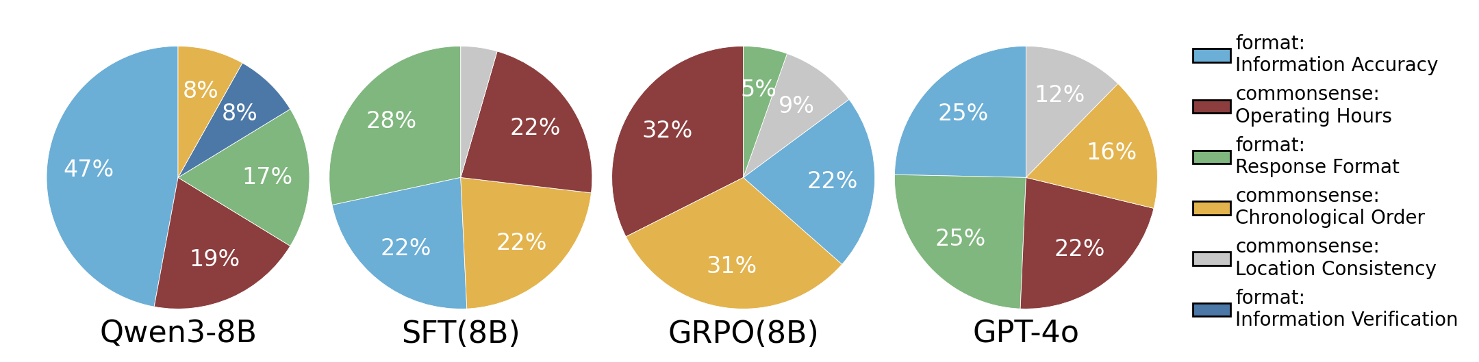
Figure 2: Format and commonsense constraints error distribution in the real-world test set.

4.4 Performance on various trip durations.

Figure 3 model performance as task complexity increases (longer trip durations). To maintain statistical significance, we focus on results for trips ranging from 1 to 5 days, excluding longer durations with insufficient data points. As the trip duration extends from 1 to 5 days, we observe a notable degradation in performance across vanilla baselines. This decline is evident in both format constraint (Average DR) and commonsense constraint (Average CPR), with a corresponding decrease in reward. In contrast, GRPO (14B), which denotes the GRPO method applied to the Qwen3-14B model, generally achieves the highest DR and CPR scores while exhibiting the smallest performance decline as trip duration increases, indicating superior stability in long-horizon planning scenarios. This suggests that GRPO improves the model’s reasoning ability for complex itineraries: it learns to maintain the consistency and constraint satisfaction (e.g., operating hours and chronological order) while preserving valid output structure, leading to stronger performance when scheduling becomes more challenging.

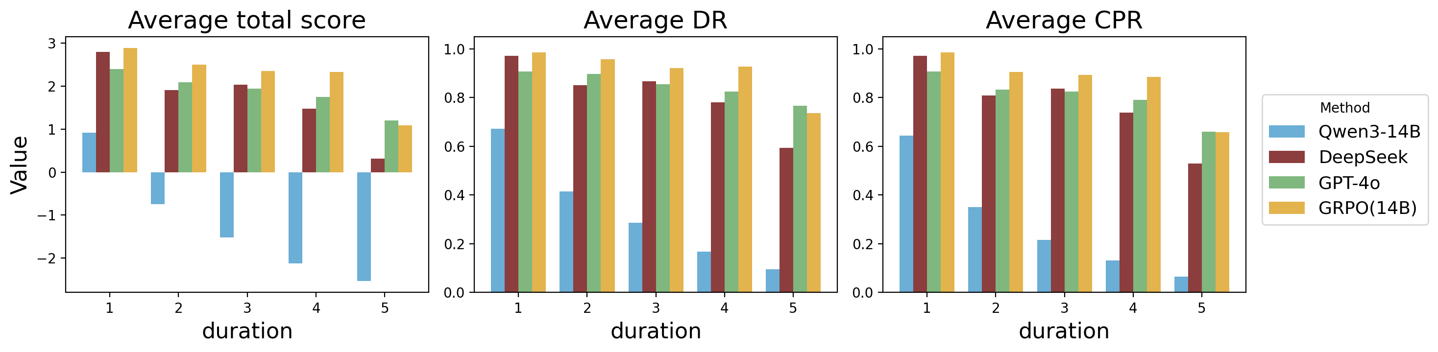
Figure 3: Performance distribution across varying trip durations in the synthetic test set.

4.5 Case Study.

To examine how itinerary quality is assessed, we present several head-to-head cases in Figure 4. Although all plans are feasible, side-by-side comparison under our criteria clearly exposes which route is superior. This underscores the need for fine-grained comparative evaluation rather than relying solely on rules or single-pass LLM judgments. Reliable evaluation must account for structural validity, spatio-temporal coherence, semantic value (iconicity and diversity), and user preferences. A practical evaluator should fuse rule-based diagnostics with preference signals, quantify uncertainty, and return actionable feedback.

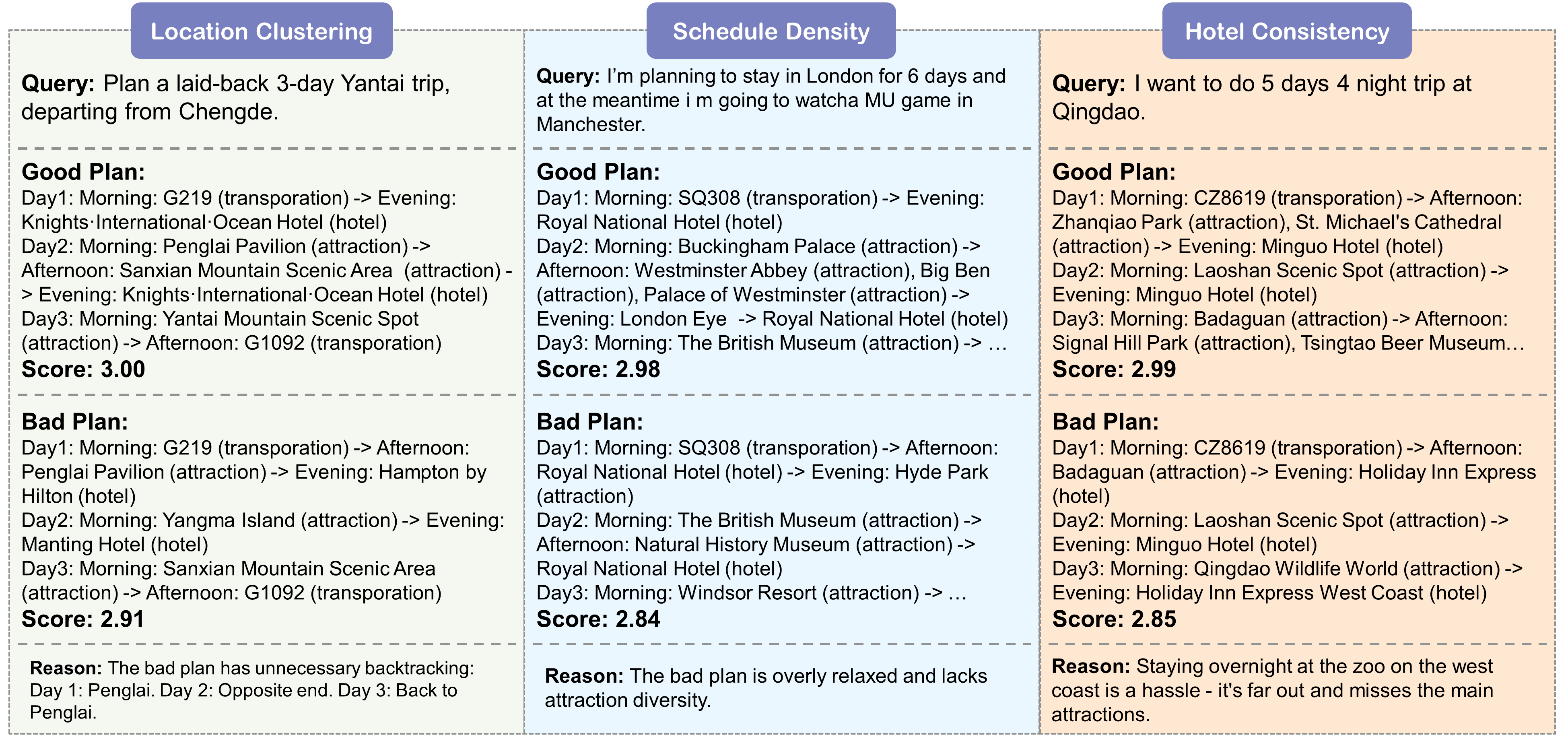
Figure 4: Case studies of the comparison of the itinerary quality.

5 Conclusion

In this work, we introduce a comprehensive evaluation framework that aggregates fine-grained criteria into a single reward for itinerary quality, achieving 60.75% agreement with expert annotations and surpassing LLM-as-judge baselines. And we also present a large-scale, real-world dataset that encapsulates authentic user requests, providing a rich resource for developing and testing travel planning systems. Finally, we conduct extensive comparative experiments that underscore the effectiveness of our framework and demonstrate the promise of fine-tuning techniques for improving itinerary quality while maintaining low inference time.

Ethics Statement

User Data Authorization. All user data utilized in this study was obtained with explicit authorization from the users. We affirm that this data is used solely for academic research purposes and will not be employed for any commercial applications.

Appendix A The Use of Large Language Models (LLMs)

In the preparation of this manuscript, large language models were employed exclusively for the purpose of writing refinement and stylistic enhancement. These models were not used for generating research ideas, conducting analyses, or drawing conclusions.

Appendix B Benchmark Details

In Table 4, we list the detailed data distribution on training, validation and test set.

Table 4: Statistics of dataset distribution. We divide the dataset into training, validation and test splits and calculate the entity number correspondingly.

Dataset	Type	#Examples	#City	#Hotel	#Attraction
Training	Synthetic	3,493	781	7,830	9,788
Validation	Synthetic	100	70	1,057	1,525
	Real-world	58	41	638	1,313
Test	Synthetic	1,000	358	4,459	5,452
	Real-world	219	122	1,894	2,057
All		4,870	897	9,376	10,997

Appendix C Expert Annotation

C.1 Expert Annotation

We conducted a comprehensive comparative evaluation, integrating expert assessments with our automated framework. We employed DeepSeek-V3, Qwen3-32B and GPT-4 to independently generate travel plans based on 3,000 user queries. After filtering out plans that failed to meet format and commonsense constraints, we obtained 1,468 final pairwise comparisons: 267 between Qwen3-32B and DeepSeek-V3, 303 between Qwen3-32B and GPT-4o, and 898 between GPT-4o and DeepSeek-V3. Then a panel of 203 travel specialists was tasked with ranking these pairs of travel plans and providing rationales for their choices. For each pair, the specialists had three options: favor route A, favor route B, or neither route met satisfactory standards. To ensure the reliability of the labeling results, each specialist was assigned routes featuring destinations with which they were familiar. And each plan pair was independently evaluated by three expert annotators.

We computed inter-annotator agreement using Cohen’s $\kappa$ for pairwise comparisons and Fleiss’ $\kappa$ for multi-rater reliability. The results demonstrated moderate agreement among the experts, with Cohen’s $\kappa$ reaching 0.5421 for pairwise comparisons and Fleiss’ $\kappa$ achieving 0.5039 for multi-rater reliability. Furthermore, we examined the agreement from different perspectives: the average pairwise agreement between annotators was 71.69%, while the overall agreement across all three raters was 59.00%.

C.2 Grid Search

We employ a grid search optimization to find the optimal weight for our evaluation framework. The search space consists of 13 parameters: 7 soft constraint weights ($w_{1}$), 4 preference weights ($w_{2}$), and 2 multiplier weights ($w_{3}$, $w_{4}$). We discretize the parameter space using coarse grids: $w_{1}\in\{0.1,0.4,0.7\}$, $w_{2}\in\{0.2,0.6,1.0\}$, $w_{3}\in\{0.8,1.0,1.2\}$, and $w_{4}\in\{0.1,0.4,0.6,0.8,1.0,1.2,1.4\}$. The optimized weight values are provide in Table 5.

We conduct stratified 5-fold cross-validation with a nested inner-loop grid search. The outer-fold validation accuracies are $[0.5933,\,0.6049,\,0.6185,\,0.5743,\,0.6466]$, yielding a mean of $0.6075\pm 0.0272$ (mean $\pm$ std). On the full 1,468-pair set, 1,000$\times$ bootstrap gives an accuracy of $0.6138$ with a 95% CI of $[0.5967,\,0.6383]$. Correlation analysis shows a positive but weak ordinal association between our model’s score differences and human preferences: train set Kendall’s $\tau{=}0.2316$; validation set Kendall’s $\tau{=}0.1892$.

C.3 Sensitive Analysis

Moreover, we probe robustness by jointly scaling the penalty multipliers $(w_{3},w_{4})\in\{(0.5,0.05),(1.0,0.10),(1.5,0.15),(2.0,0.20)\}$ and by applying simplex normalization (including temperature smoothing) to the soft and preference constraint weights. Across all variants, train agreement remains in the range 59.40%-62.26% and validation agreement in 58.47%-61.32%, i.e., within $\approx\!2.8$ pp (train) and $\approx\!2.9$ pp (val) absolute of the baseline. The near-constant validation accuracy under multiplier scaling and simplex reparameterizations indicates the method is robust to these design choices and does not rely on a narrow hyperparameter configuration.

Table 5: Optimized weights value. Due to the different evaluation method, synthetic and real-world datasets share the weights for soft constraints but utilize distinct preference weights.

Parameter		Synthetic	Real-world
w1 (soft constraints)	Schedule Density	0.70
	Hotel Consistency	0.50
	Daytime Utilization	0.40
	Unique Attraction	0.20
	Location Clustering	0.70
	Iconic Landmark	0.10
	Attraction Diversity	0.20
w2 (preferences)	Attraction Prioritization	0.20	-
	Pacing	0.60	-
	Budget	0.60	-
	Physical Effort	0.60	-
	User Request	-	1.00
w3 (soft constraint multiplier)		1.00
w4 (preference multiplier)		0.10	1.40

C.4 Noise-adjusted Analysis

Under a standard K-class symmetric-noise model, we can relate the average human-human pairwise agreement $A_{\text{pair}}$ and a typical annotator’s agreement with respect to the latent truth $r$ as follows:

$$A_{\text{pair}}=r^{2}+\frac{(1-r)^{2}}{K-1}$$ (4)

$$r=\frac{1+\sqrt{(K-1)(K\cdot A_{\text{pair}}-1)}}{K}$$ (5)

Where $K$ is the number of classes. With $K=3$ and $A_{\text{pair}}=0.7169$, we calculate the human reliability ceiling, $r\approx 0.8390$. Then the expected model-human agreement $A_{\text{model},h}$ relates to the model’s latent-truth agreement $r_{\text{model}}$ by:

$$A_{\text{model},h}=r_{\text{model}}\cdot r+\frac{(1-r_{\text{model}})(1-r)}{K-1}$$ (6)

Which can be rearranged to solve for $r_{\text{model}}$:

$$r_{\text{model}}=\frac{K\cdot A_{\text{model},h}-A_{\text{model},h}+r-1}{K\cdot r-1}$$ (7)

Substituting $A_{\text{model},h}=0.6075$, $K=3$ and $r\approx 0.8390$ yields $r_{\text{model}}\approx 0.695$. Thus, the raw 60.75% agreement corresponds to a noise-adjusted latent agreement of approximately 69.5%. We can express this as a ratio of the model’s performance to the human reliability ceiling $r_{\text{model}}/r\approx 0.828$. This indicates that the model achieves about 82.8% of the human reliability ceiling.

As a verification, we can also calculate the predicted three-annotator all-agree rate $A_{\text{all}}$ by the calculated human reliability ceiling $r$:

$$A_{\text{all}}=r^{3}+\frac{(1-r)^{3}}{(K-1)^{2}}\approx 0.594$$ (8)

This closely matches the observed overall agreement of 0.590 between all annotators, providing a sanity check for our calculations.

C.5 Evaluation Comparison Experiments

We implement two LLM-as-judge paradigms to evaluate pairs of candidate itineraries and evaluate agreement with expert labels as well as rank correlation (Kendall’s $\tau$). Both paradigms use a structured rubric of hard/soft constraints and explicitly condition on the user request. To improve reproducibility, we use frozen prompts, temperature 0, and report results across 3 runs. And we report the results for multiple LLMs (GPT-4o, GPT-4.1-Mini, DeepSeek-V3-0324, Gemini-2.5-flash/pro).

Point-wise scoring. The LLM independently scores each itinerary in $[0,100]$ under the same request and rubric. To mitigate instability reported in prior work (Bai et al., 2023), we adopt comparative prompting, anchoring scores with comparative references. The predicted winner is the itinerary with the higher score; ties yield a neither decision. We report two point-wise metrics: tie-excluded accuracy and tie-inclusive accuracy. The full prompt is provided in Appendix H.5.

Pair-wise comparison. The LLM receives the request and both itineraries, first eliminates candidates with hard-constraint violations, then compares soft quality and preference matching; if still uncertain, it selects the clearer, more executable plan. The model must output exactly one token from route A, route B. The prompt is provided in Appendix H.6.

Ours scoring method. For our rule-and-LLM-hybrid evaluation framework, we have the same setting as point-wise scoring: the predicted winner is the itinerary with the higher score, and ties yield neither decision. We employ various LLMs for the LLM-based component. Because tie-excluded and tie-inclusive accuracies are nearly identical, we report only the tie-inclusive accuracy in Table 6.

Table 6: Comparison with human annotations for our method and LLM-as-judge baselines. For point-wise results, values in parentheses indicate tie-inclusive accuracies.

Method	LLM	Accuracy	Kendall’s $\tau$
Point-wise	Gemini-2.5-flash	61.42 (49.77)	0.2182
	Gemini-2.5-pro	62.35 (53.05)	0.2347
	GPT-4.1-Mini	47.01 (34.74)	-0.0224
	GPT-4o	53.05 (36.15)	0.0466
	DeepSeek-V3	51.02 (29.76)	0.0193
Pair-wise	Gemini-2.5-flash	57.94	0.1529
	Gemini-2.5-pro	58.77	0.1675
	GPT-4.1-Mini	49.53	-0.0795
	GPT-4o	53.27	0.0762
	DeepSeek-V3	51.64	0.0104
Ours	Gemini-2.5-flash	60.75	0.1892
	Gemini-2.5-pro	61.32	0.2124
	GPT-4o	57.94	0.1488
	DeepSeek-V3	56.48	0.1196

Appendix D Experiment Details

D.1 Fine tuning

SFT. We fine‑tune the pretrained model with pairwise query–response supervision. The SFT training set is constructed by prompting GPT‑4o to answer queries from the synthetic training split. Then we filter out samples that violate our format or commonsense constraints. This yields 2,094 training and 71 validation examples. As GPT-4o does not expose an explicit chain-of-thought, we train the base model in a non-thinking configuration. During training, we set the maximum sequence length to 115,000 tokens and training epochs to 3. As the context length is too long, which may lead to GPU out of memory, we set the sequence parallel to 8 to ensure training progress.

RFT (Yuan et al., 2023). We further refine the SFT-tuned Qwen3-8B models via RFT. Starting from the queries in the synthesis training split, we prompt the SFT model to generate five candidate routes per query and score each route with our own evaluator. The highest-scoring route is retained; queries for which all five candidates fail the quality bar are dropped. This curation leaves 2,372 clean training samples. We then fine-tune the SFT model for three epochs on this set, using the same hyperparameters as SFT.

GRPO (Shao et al., 2024b). The detailed explanation of GRPO is provided in Appendix E. We train the SFT model based on GRPO algorithm on queries from the synthetic training set. Given that the SFT model was trained without a thinking mode, we preserve this setting and continue fine-tuning it using the GRPO algorithm. For each query, the policy model generates 8 rollouts, and rewards are computed by our evaluation framework. To speed up training, we use only the rule‑based components of the evaluator. During training process, the maximum prompt length is 79000 and the maximum answer length is 7000.

We perform early stopping by selecting the best-performing checkpoint for each task independently. The hyperparameters employed in fine-tuning baselines are presented in Table 7.

Table 7: The hyperparameters we employ in baselines.

Method	Hyperparameter	value
SFT	learning rate	1e-5
	scheduler type	cosine
	batch size	1
	training epoch	3
	warmup ratio	0.1
RFT	learning rate	1e-5
	scheduler type	cosine
	batch size	1
	training epoch	3
	warmup ratio	0.1
GRPO	actor learning rate	1e-6
	scheduler type	constant
	batch size	24
	training epoch	1
	rollout temperature	1.2
	rollout times	8

For deployment, we leverage vLLM (Kwon et al., 2023) to serve both Qwen3-8B and Qwen3-14B. To maximize inference throughput, we configure tensor parallelism to 8 and run the models on a single 8×A100 node.

D.2 Other Baselines

Direct. This approach involves inputting the query directly into the model, accompanied by comprehensive instructions detailing the task requirements and all relevant gathered information. The model is expected to generate a response based solely on this input. For Qwen3-8B, we disable the thinking mode for the direct method.

Zero-Shot Chain-of-Thought (ZS-CoT) (Wei et al., 2022). This method enhances the reasoning process by encouraging the model to articulate intermediate steps. Building upon the Direct method, we augment the prompt with the phrase “Let’s think step by step.” This addition is designed to elicit a more detailed, structured reasoning process from the model, potentially leading to more accurate and transparent outcomes. For Qwen3-8B, we enable the thinking mode for the ZS-COT method.

TTG (Ju et al., 2024). TTG (To The Globe) is a hybrid travel-planning system that translates natural language requests into structured JSON constraints using a fine-tuned LLM. It then solves these constraints with a Mixed Integer Linear Programming (MILP) solver to guarantee feasible and near-optimal itineraries in under 5 seconds. It combines the LLMs’ natural language abilities with the mathematical guarantees of MILP solvers.

To implement TTG into our benchmark, we define a symbolic type to represent feasible travel constraints, serving as the intermediate format for MILP problem generation. Then we translate travel requests into MILP formulations that encode itinerary feasibility and optimization objectives. Finally, we integrate the Python PuLP library to solve the constructed MILP problems using appropriate solver strategies.

NESY (Shao et al., 2024a). The NESY baseline scheme consists of a two-stage process: (1) In the NL2DSL translation stage, natural language queries are converted into logical and preference DSL requirements; (2) In the interactive search stage, a neuro-symbolic solver sequentially arranges activities under the guidance of a symbolic sketch and LLM-driven POI recommendations, generating a multi-day itinerary with DSL validation.

To adapt NESY to our dataset, we implement the following modifications:

• Dataset Adaptation. We streamline the planning process by removing redundant logical modules irrelevant to our study, such as restaurants, ensuring the workflow aligns with the available data support.

• DSL and Concept Function Reconstruction. We reconstruct the concept functions and augmented the DSL statements with commonsense constraints to match the specific format of our itinerary results. Specifically, we removed DSL statements related to restaurants, people number, dishes, and room types, while expanding commonsense constraints. Ultimately, 32 concept functions were obtained, and the input of each function includes the planned itinerary elements as well as relevant information.

• Multi-Destination Planning. To address the limitations of the original NESY framework, which only supported single-destination planning and lacked mechanisms for sequencing multiple destinations, we implement a two-phase modification: (1) For determining the destination sequence, we prioritize transportation data (e.g. direct accessibility, travel duration) to determine the planning order. In the absence of such data, we default to the sequence extracted from user input via LLMs. (2) For day allocation, we introduce a “cyclic allocation method”: each destination is initially assigned one day, with additional days distributed sequentially according to the predetermined order until meeting the total day requirement.

• Transportation Mode Adaptation. To address the original method’s limitation of deeming planning infeasible when large-scale transportation data (e.g. flights, trains) are unavailable, we implement a more flexible approach. In the absence of such data, we now default to a “self-driving” mode. This adaptation accommodates scenarios like local trips and self-driving tours, maximizing the utilization of POI resources in areas lacking comprehensive transportation data. We establish fixed time windows for self-driving based on typical travel patterns: outbound trips are scheduled from 9:00 to 11:00, and return trips from 18:00 to 20:00.

LLM-Modulo (Kambhampati et al., 2024). LLM-Modulo is a hybrid method where a large language model (LLM) generates structured representations from a user’s request, and a symbolic planner verifies them and flags issues in a feedback loop. The method benefits from the bidirectional interaction: The symbolic module actively gives feedback to the LLM, and the LLM refines the itinerary iteratively.

To implement the LLM-Modulo into our benchmark, we develop specialized prompts to guide the LLM in generating initial itineraries and refining them based on evaluator feedback. We reuse our existing constraint evaluators to automatically score itineraries and provide structured feedback to the LLM, and for fairness we only utilize the rule-based part in our evaluation framework. We also add a controller that coordinates iterations between the LLM and the evaluators until constraints are satisfied or a timeout is reached. We set a maximum of 3 iteration steps and stop the refinement process if the reward score exceeds 3.5.

HyperTree (Gui et al., 2025). This baseline employs a hypertree-structured reasoning paradigm that recursively decomposes a travel query into transportation, accommodation, and attraction subtasks. By employing this recursive decomposition strategy, the baseline ensures that each aspect of the travel plan can be meticulously crafted and seamlessly integrated, resulting in a highly personalized and adaptable itinerary.

To adapt HyperTree to our dataset, we implement several modifications. We remove all the hypertree rules and nodes related to Dining to align with our schema. We also refactor the hypertree library to handle an arbitrary-length destination list, dynamically generating city-specific subtrees and their corresponding inter-city transportation segments, with no upper bound on the number of cities. Additionally, as the repository does not provide prompts, we write them from scratch based on the descriptions in the paper.

Appendix E Reinforcement Learning

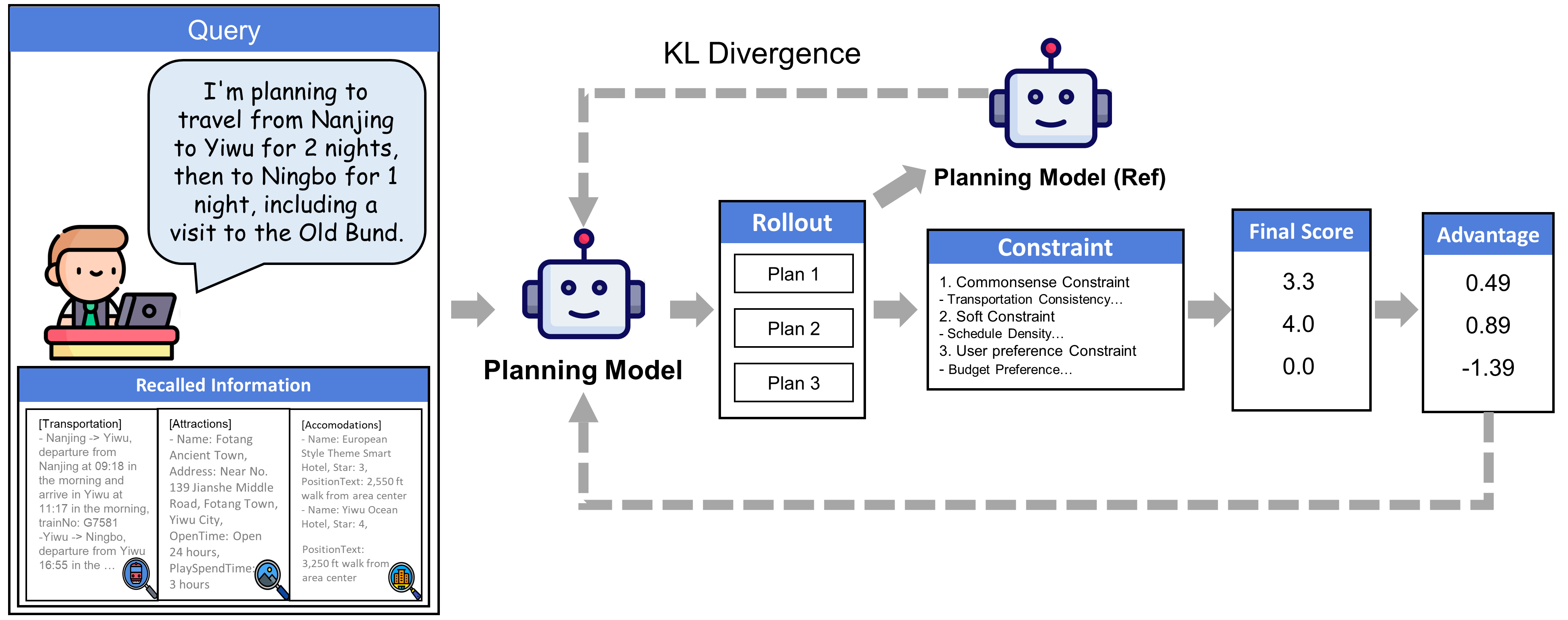
Figure 5: Demonstration of the Grouped Relative Policy Optimization (GRPO). GRPO estimates the baseline from group scores, and normalize them into a standard value. The planning model undergoes iterative optimization by maximizing the objective function $\mathcal{L}(\pi_{\theta})$.

We leverage reinforcement learning to enhance the reasoning capabilities of Large Language Models (LLMs) for travel planning. We implement the Grouped Relative Policy Optimization (GRPO) (Shao et al., 2024b) algorithm, as illustrated in Figure 5. This approach is well-suited for our travel planning task due to its ability to handle fine-grained ordinal reward.

For each user query $q$, we sample a group of travel plans $\{o_{1},o_{2},\ldots,o_{G}\}$, from the current planning model $\pi_{\theta_{\text{old}}}$. These plans are then evaluated by our framework, which assigns a reward score to each plan $r=\{r_{1},r_{2},\ldots,r_{G}\}$. To improve training efficiency, we utilize only the rule-based component of our evaluation, omitting the LLM-based assessment. We normalize these rewards within each group $\tilde{r}_{i}=(r_{i}-\mathrm{mean}(r))/\mathrm{std}(r)$. For each plan $o_{i}$ in the group, we set the advantage $\hat{A}_{i,t}$, for all tokens in the plan as the normalized reward $\hat{A}_{i,t}=\tilde{r}_{i}$. The planning model is then optimized by maximizing the objective $\mathcal{L}(\pi_{\theta})$.

$$r_{i,t}(\theta)\coloneqq\frac{\pi_{\theta}(o_{i,t}\mid q,\,o_{i,<t})}{\pi_{\theta_{\text{old}}}(o_{i,t}\mid q,\,o_{i,<t})}$$ (9)

$$\mathcal{L}(\pi_{\theta})=\frac{1}{G}\sum_{i=1}^{G}\frac{1}{|o_{i}|}\sum_{t=1}^{|o_{i}|}\!\left\{\min\!\left[r_{i,t}(\theta)\hat{A}_{i,t},\;\text{clip}\bigl(r_{i,t}(\theta),1\!-\!\varepsilon,1\!+\!\varepsilon\bigr)\hat{A}_{i,t}\right]\!-\!\beta D_{\mathrm{KL}}\!\left[\pi_{\theta}\ \|\pi_{\text{ref}}\right]\right\}$$ (10)

where $\beta$ serves as a coefficient that regulates the influence of the KL divergence constraint and $\varepsilon$ is a hyperparameter that determines the extent of the clipping in the surrogate objective.

Appendix F Soft Constraint Score Rule

The soft constraints $\bm{S_{\text{soft}}}$ encompass schedule density, hotel consistency, daytime utilization, unique attractions, location clustering, iconic landmark, and attraction diversity. Formally, $\bm{S_{\text{soft}}}=(S_{\text{schedule}},S_{\text{hotel}},S_{\text{daytime}},S_{\text{unique}},S_{\text{location}},S_{\text{iconic}},S_{\text{diversity}})$.

1. Schedule Density. This metric assesses the temporal feasibility of daily itineraries by checking minimum and maximum activity hours against day-specific thresholds. Scoring is by day-level violation (at most one penalty per day):

$$S_{\text{schedule}}=1-\frac{|d_{v}|}{D}$$ (11)

where $D$ is the total number of days. $d_{v}$ is the set of days where the total activity hours exceed the upper bound or fall below the lower bound.

2. Hotel Consistency. The hotel consistency metric applies penalties to unnecessary hotel changes within a single city:

$$S_{\text{hotel}}=1-\frac{|S_{\text{switches}}|}{|H|}$$ (12)

where $S_{\text{switches}}$ represents the number of nights involving a switch to a nearby hotel (within 100 km) in the same city, and $|H|$ is the total number of hotel nights.

3. Daytime Utilization. This constraint ensures the efficient utilization of daytime hours, with a focus on avoiding idle time or overcrowded scheduling:

$$S_{\text{daytime}}=1-\frac{\sum_{d=1}^{D}\mathbf{1}[\text{violation}_{d}]}{D}$$ (13)

where $\text{violation}_{d}$ occurs when there is not arranged any activities in the morning and afternoon.

4. Unique Attractions. The uniqueness score employs a combination of linear and exponential penalties to quantify the degree of redundancy among selected attractions:

$$S_{\text{unique}}=\max\left(0,1-\frac{|A_{\text{dup}}|}{|A_{\text{total}}|}-\sum_{a\in A_{\text{dup}}}\frac{(n_{a}-1)^{2}\cdot 0.05}{|A_{\text{total}}|}\right)$$ (14)

where $A_{\text{dup}}$ represents non-consecutively duplicated attractions. $n_{a}$ is the number of times an activity appears. $A_{\text{total}}$ represents the total attractions in the itinerary.

5. Location Clustering. This metric optimizes the spatial distribution of daily activities by applying penalties proportional to inter-attraction distances:

$$S_{\text{location}}=\max\left(0,1-\frac{\mathcal{P}_{\text{total}}}{|A_{\text{total}}|}$$ (15)

where $\mathcal{P}_{\text{total}}$ represents the consecutive activity pairs for the same day that are among the top 20% farthest of all activity pairs.

6. Iconic Landmark and Attraction Diversity. These two metrics are assessed using a 5-point Likert scale, with evaluations conducted by LLMs. The resulting scores are then normalized to ensure they fall within the range of 0 to 1. The corresponding prompts are provided in Appendix H.2 and Appendix H.1. The calculation applied to both the Iconic Landmark and Attraction Diversity metrics is as follows.

$$S=\frac{\text{rating}-1}{4},\quad\text{rating}\in{1,2,3,4,5}$$ (16)

This formulation ensures that the lowest rating (1) corresponds to a normalized score of 0, while the highest rating (5) yields a normalized score of 1, providing a standardized measure for both iconic landmarks and attraction diversity.

Appendix G Preference Constraint Score Rule

Synthesis Datasets. The preference evaluator measures how well an itinerary aligns with the user’s stated preferences. We consider four dimensions: $\bm{S_{\text{pref}}}=(S_{\text{budget}},S_{\text{pacing}},S_{\text{attraction}},S_{\text{effort}})$.

1. Budget Preference ($E_{budget}$): The budget preference metric calculates the proportion of consistency between users’ budget-corresponding expected hotel star ratings and actual hotel star ratings, aiming to measure the matching degree of budget and hotel star:

$$S_{\text{budget}}=\frac{1}{|H|}\sum_{h\in H}g(h;\,\text{pref}).$$ (17)

where $H$ is the set of hotel nights, and $g(h;\,\text{pref})\in\{0,1\}$ indicate whether night $h$ matches the budget preference (e.g., 0-2 stars for ”cost-effective”, 3-4 stars for ”comfortable” and 5 stars for ”High-end”).

2. Pacing Preference ($E_{\text{pacing}}$): Pacing Preference quantifies the consistency between the actual itinerary arrangement and users’ pace preferences based on key indicators such as play duration and the number of activities:

$$S_{\text{pacing}}=\frac{1}{D}\sum_{d=1}^{D}f(d;\,\text{pref}).$$ (18)

where $D$ is the number of days and $f(d;\,\text{pref})\in[0,1]$ is a day-level compliance function (1 when daily maximum or minimum activity time thresholds are met, intermediate value otherwise)

3. Attraction Preference ($E_{\text{attraction}}$): We map user attraction preferences to POI tags and measure coverage among visited POIs. It is calculated by the proportion of qualified attraction:

$$S_{\text{attraction}}=\frac{1}{|A_{\text{total}}|}\sum_{a\in A_{\text{total}}}m(a;\,\text{pref}).$$ (19)

where $A_{\text{total}}$ represents all visited attractions and $m(a;\,\text{pref})\in\{0,1\}$ indicating whether attraction $a$ matches any preferred tag.

4. Physical Effort Preference ($E_{\text{effort}}$): Calculates activity’s physical effort value by rules, determines itinerary exertion type via high-effort activity and duration ratios, and quantifies consistency with users’ physical effort preferences.

$$S_{\text{attraction}}=\frac{1}{D}\sum_{d=1}^{D}h(d;\,\text{pref}).$$ (20)

where $h(d;\,\text{pref})\in\{0,1\}$ indicate whether the day $d$ matches the preferred physical effort tag. A day is labeled strenuous if (i) its single‑day physical‑exertion score is greater than 2, where hiking, theme-park and mountain-climbing each contribute 1, cycling contributes 2, and all other activities contribute 0; or (ii) it requires physical exertion on two consecutive days. A day is light if it involves no exertion and neither adjacent day involves exertion. All remaining cases are moderate.

Real-world Datasets. For real-world datasets, we employ LLM-based evaluation to assess overall user request compliance. $S_{pref}=\{S_{user}\}$. The corresponding prompt is provided in Appendix H.3.

$$S_{user}=\alpha\text{LLM}(\text{prompt},\text{response},\text{user\_request})$$ (21)

where $\alpha$ represents the scaling weight (0.2) employed to normalize the score within the range of 0 to 1.

Appendix H Prompt List

H.1 Iconic Landmarks Evaluation Prompt

H.2 Attraction Diversity Evaluation Prompt

H.3 User Request Fulfillment Evaluation Prompt

H.4 Itinerary Generation Prompt

H.5 Point-wise evaluation Prompt

H.6 Pair-wise evaluation Prompt

References

- Anil et al. (2023) Rohan Anil, Sebastian Borgeaud, Yonghui Wu, Jean-Baptiste Alayrac, Jiahui Yu, Radu Soricut, Johan Schalkwyk, Andrew M. Dai, Anja Hauth, Katie Millican, David Silver, Slav Petrov, Melvin Johnson, Ioannis Antonoglou, Julian Schrittwieser, Amelia Glaese, Jilin Chen, Emily Pitler, Timothy P. Lillicrap, Angeliki Lazaridou, Orhan Firat, James Molloy, Michael Isard, Paul Ronald Barham, Tom Hennigan, Benjamin Lee, Fabio Viola, Malcolm Reynolds, Yuanzhong Xu, Ryan Doherty, Eli Collins, Clemens Meyer, Eliza Rutherford, Erica Moreira, Kareem Ayoub, Megha Goel, George Tucker, Enrique Piqueras, Maxim Krikun, Iain Barr, Nikolay Savinov, Ivo Danihelka, Becca Roelofs, Anaïs White, Anders Andreassen, Tamara von Glehn, Lakshman Yagati, Mehran Kazemi, Lucas Gonzalez, Misha Khalman, Jakub Sygnowski, and et al. Gemini: A family of highly capable multimodal models. CoRR, abs/2312.11805, 2023. doi: 10.48550/ARXIV.2312.11805. URL https://doi.org/10.48550/arXiv.2312.11805.
- Bai et al. (2023) Yushi Bai, Jiahao Ying, Yixin Cao, Xin Lv, Yuze He, Xiaozhi Wang, Jifan Yu, Kaisheng Zeng, Yijia Xiao, Haozhe Lyu, Jiayin Zhang, Juanzi Li, and Lei Hou. Benchmarking foundation models with language-model-as-an-examiner. In Alice Oh, Tristan Naumann, Amir Globerson, Kate Saenko, Moritz Hardt, and Sergey Levine (eds.), Advances in Neural Information Processing Systems 36: Annual Conference on Neural Information Processing Systems 2023, NeurIPS 2023, New Orleans, LA, USA, December 10 - 16, 2023, 2023. URL http://papers.nips.cc/paper_files/paper/2023/hash/f64e55d03e2fe61aa4114e49cb654acb-Abstract-Datasets_and_Benchmarks.html.
- Chen et al. (2024) Aili Chen, Xuyang Ge, Ziquan Fu, Yanghua Xiao, and Jiangjie Chen. Travelagent: An AI assistant for personalized travel planning. CoRR, abs/2409.08069, 2024. doi: 10.48550/ARXIV.2409.08069. URL https://doi.org/10.48550/arXiv.2409.08069.
- Chen et al. (2023) Wenhu Chen, Ming Yin, Max Ku, Pan Lu, Yixin Wan, Xueguang Ma, Jianyu Xu, Xinyi Wang, and Tony Xia. Theoremqa: A theorem-driven question answering dataset. In Houda Bouamor, Juan Pino, and Kalika Bali (eds.), Proceedings of the 2023 Conference on Empirical Methods in Natural Language Processing, EMNLP 2023, Singapore, December 6-10, 2023, pp. 7889–7901. Association for Computational Linguistics, 2023. doi: 10.18653/V1/2023.EMNLP-MAIN.489. URL https://doi.org/10.18653/v1/2023.emnlp-main.489.
- Cobbe et al. (2021) Karl Cobbe, Vineet Kosaraju, Mohammad Bavarian, Mark Chen, Heewoo Jun, Lukasz Kaiser, Matthias Plappert, Jerry Tworek, Jacob Hilton, Reiichiro Nakano, Christopher Hesse, and John Schulman. Training verifiers to solve math word problems. CoRR, abs/2110.14168, 2021. URL https://arxiv.org/abs/2110.14168.
- DeepSeek-AI et al. (2025) DeepSeek-AI, Daya Guo, Dejian Yang, Haowei Zhang, Junxiao Song, Ruoyu Zhang, Runxin Xu, Qihao Zhu, Shirong Ma, Peiyi Wang, Xiao Bi, Xiaokang Zhang, Xingkai Yu, Yu Wu, Z. F. Wu, Zhibin Gou, Zhihong Shao, Zhuoshu Li, Ziyi Gao, Aixin Liu, Bing Xue, Bingxuan Wang, Bochao Wu, Bei Feng, Chengda Lu, Chenggang Zhao, Chengqi Deng, Chenyu Zhang, Chong Ruan, Damai Dai, Deli Chen, Dongjie Ji, Erhang Li, Fangyun Lin, Fucong Dai, Fuli Luo, Guangbo Hao, Guanting Chen, Guowei Li, H. Zhang, Han Bao, Hanwei Xu, Haocheng Wang, Honghui Ding, Huajian Xin, Huazuo Gao, Hui Qu, Hui Li, Jianzhong Guo, Jiashi Li, Jiawei Wang, Jingchang Chen, Jingyang Yuan, Junjie Qiu, Junlong Li, J. L. Cai, Jiaqi Ni, Jian Liang, Jin Chen, Kai Dong, Kai Hu, Kaige Gao, Kang Guan, Kexin Huang, Kuai Yu, Lean Wang, Lecong Zhang, Liang Zhao, Litong Wang, Liyue Zhang, Lei Xu, Leyi Xia, Mingchuan Zhang, Minghua Zhang, Minghui Tang, Meng Li, Miaojun Wang, Mingming Li, Ning Tian, Panpan Huang, Peng Zhang, Qiancheng Wang, Qinyu Chen, Qiushi Du, Ruiqi Ge, Ruisong Zhang, Ruizhe Pan, Runji Wang, R. J. Chen, R. L. Jin, Ruyi Chen, Shanghao Lu, Shangyan Zhou, Shanhuang Chen, Shengfeng Ye, Shiyu Wang, Shuiping Yu, Shunfeng Zhou, Shuting Pan, and S. S. Li. Deepseek-r1: Incentivizing reasoning capability in llms via reinforcement learning. CoRR, abs/2501.12948, 2025. doi: 10.48550/ARXIV.2501.12948. URL https://doi.org/10.48550/arXiv.2501.12948.
- Gui et al. (2025) Runquan Gui, Zhihai Wang, Jie Wang, Chi Ma, Hui-Ling Zhen, Mingxuan Yuan, Jianye Hao, Defu Lian, Enhong Chen, and Feng Wu. Hypertree planning: Enhancing LLM reasoning via hierarchical thinking. CoRR, abs/2505.02322, 2025. doi: 10.48550/ARXIV.2505.02322. URL https://doi.org/10.48550/arXiv.2505.02322.
- Hao et al. (2023) Shibo Hao, Yi Gu, Haodi Ma, Joshua Jiahua Hong, Zhen Wang, Daisy Zhe Wang, and Zhiting Hu. Reasoning with language model is planning with world model. In Houda Bouamor, Juan Pino, and Kalika Bali (eds.), Proceedings of the 2023 Conference on Empirical Methods in Natural Language Processing, EMNLP 2023, Singapore, December 6-10, 2023, pp. 8154–8173. Association for Computational Linguistics, 2023. doi: 10.18653/V1/2023.EMNLP-MAIN.507. URL https://doi.org/10.18653/v1/2023.emnlp-main.507.
- Hao et al. (2025) Yilun Hao, Yongchao Chen, Yang Zhang, and Chuchu Fan. Large language models can solve real-world planning rigorously with formal verification tools. In Luis Chiruzzo, Alan Ritter, and Lu Wang (eds.), Proceedings of the 2025 Conference of the Nations of the Americas Chapter of the Association for Computational Linguistics: Human Language Technologies (Volume 1: Long Papers), pp. 3434–3483, Albuquerque, New Mexico, April 2025. Association for Computational Linguistics. ISBN 979-8-89176-189-6. doi: 10.18653/v1/2025.naacl-long.176. URL https://aclanthology.org/2025.naacl-long.176/.
- Hu et al. (2025) Lanxiang Hu, Qiyu Li, Anze Xie, Nan Jiang, Ion Stoica, Haojian Jin, and Hao Zhang. Gamearena: Evaluating LLM reasoning through live computer games. In The Thirteenth International Conference on Learning Representations, ICLR 2025, Singapore, April 24-28, 2025. OpenReview.net, 2025. URL https://openreview.net/forum?id=SeQ8l8xo1r.
- Jain et al. (2025) Naman Jain, King Han, Alex Gu, Wen-Ding Li, Fanjia Yan, Tianjun Zhang, Sida Wang, Armando Solar-Lezama, Koushik Sen, and Ion Stoica. Livecodebench: Holistic and contamination free evaluation of large language models for code. In The Thirteenth International Conference on Learning Representations, ICLR 2025, Singapore, April 24-28, 2025. OpenReview.net, 2025. URL https://openreview.net/forum?id=chfJJYC3iL.
- Jimenez et al. (2024) Carlos E. Jimenez, John Yang, Alexander Wettig, Shunyu Yao, Kexin Pei, Ofir Press, and Karthik R. Narasimhan. Swe-bench: Can language models resolve real-world github issues? In The Twelfth International Conference on Learning Representations, ICLR 2024, Vienna, Austria, May 7-11, 2024. OpenReview.net, 2024. URL https://openreview.net/forum?id=VTF8yNQM66.
- Ju et al. (2024) Da Ju, Song Jiang, Andrew Cohen, Aaron Foss, Sasha Mitts, Arman Zharmagambetov, Brandon Amos, Xian Li, Justine T Kao, Maryam Fazel-Zarandi, and Yuandong Tian. To the globe (TTG): Towards language-driven guaranteed travel planning. In Delia Irazu Hernandez Farias, Tom Hope, and Manling Li (eds.), Proceedings of the 2024 Conference on Empirical Methods in Natural Language Processing: System Demonstrations, pp. 240–249, Miami, Florida, USA, November 2024. Association for Computational Linguistics. doi: 10.18653/v1/2024.emnlp-demo.25. URL https://aclanthology.org/2024.emnlp-demo.25/.
- Kambhampati et al. (2024) Subbarao Kambhampati, Karthik Valmeekam, Lin Guan, Mudit Verma, Kaya Stechly, Siddhant Bhambri, Lucas Saldyt, and Anil Murthy. Position: Llms can’t plan, but can help planning in llm-modulo frameworks. In Forty-first International Conference on Machine Learning, ICML 2024, Vienna, Austria, July 21-27, 2024. OpenReview.net, 2024. URL https://openreview.net/forum?id=Th8JPEmH4z.
- Kwon et al. (2023) Woosuk Kwon, Zhuohan Li, Siyuan Zhuang, Ying Sheng, Lianmin Zheng, Cody Hao Yu, Joseph Gonzalez, Hao Zhang, and Ion Stoica. Efficient memory management for large language model serving with pagedattention. In Proceedings of the 29th Symposium on Operating Systems Principles, SOSP ’23, pp. 611–626, New York, NY, USA, 2023. Association for Computing Machinery. ISBN 9798400702297. doi: 10.1145/3600006.3613165. URL https://doi.org/10.1145/3600006.3613165.
- Nguyen et al. (2025) Dung Manh Nguyen, Thang Chau Phan, Nam Le Hai, Tien-Thong Doan, Nam V. Nguyen, Quang Pham, and Nghi D. Q. Bui. Codemmlu: A multi-task benchmark for assessing code understanding & reasoning capabilities of codellms. In The Thirteenth International Conference on Learning Representations, ICLR 2025, Singapore, April 24-28, 2025. OpenReview.net, 2025. URL https://openreview.net/forum?id=CahIEKCu5Q.
- OpenAI (2023) OpenAI. GPT-4 technical report. CoRR, abs/2303.08774, 2023. doi: 10.48550/ARXIV.2303.08774. URL https://doi.org/10.48550/arXiv.2303.08774.
- Paglieri et al. (2025) Davide Paglieri, Bartlomiej Cupial, Samuel Coward, Ulyana Piterbarg, Maciej Wolczyk, Akbir Khan, Eduardo Pignatelli, Lukasz Kucinski, Lerrel Pinto, Rob Fergus, Jakob Nicolaus Foerster, Jack Parker-Holder, and Tim Rocktäschel. BALROG: benchmarking agentic LLM and VLM reasoning on games. In The Thirteenth International Conference on Learning Representations, ICLR 2025, Singapore, April 24-28, 2025. OpenReview.net, 2025. URL https://openreview.net/forum?id=fp6t3F669F.
- Pan et al. (2024) Yichen Pan, Dehan Kong, Sida Zhou, Cheng Cui, Yifei Leng, Bing Jiang, Hangyu Liu, Yanyi Shang, Shuyan Zhou, Tongshuang Wu, and Zhengyang Wu. Webcanvas: Benchmarking web agents in online environments. CoRR, abs/2406.12373, 2024. doi: 10.48550/ARXIV.2406.12373. URL https://doi.org/10.48550/arXiv.2406.12373.
- Rawles et al. (2023) Christopher Rawles, Alice Li, Daniel Rodriguez, Oriana Riva, and Timothy P. Lillicrap. Androidinthewild: A large-scale dataset for android device control. In Alice Oh, Tristan Naumann, Amir Globerson, Kate Saenko, Moritz Hardt, and Sergey Levine (eds.), Advances in Neural Information Processing Systems 36: Annual Conference on Neural Information Processing Systems 2023, NeurIPS 2023, New Orleans, LA, USA, December 10 - 16, 2023, 2023. URL http://papers.nips.cc/paper_files/paper/2023/hash/bbbb6308b402fe909c39dd29950c32e0-Abstract-Datasets_and_Benchmarks.html.
- Shao et al. (2024a) Jie-Jing Shao, Xiao-Wen Yang, Bo-Wen Zhang, Baizhi Chen, Wen-Da Wei, Guohao Cai, Zhenhua Dong, Lan-Zhe Guo, and Yu-feng Li. Chinatravel: A real-world benchmark for language agents in chinese travel planning. CoRR, abs/2412.13682, 2024a. doi: 10.48550/ARXIV.2412.13682. URL https://doi.org/10.48550/arXiv.2412.13682.
- Shao et al. (2024b) Zhihong Shao, Peiyi Wang, Qihao Zhu, Runxin Xu, Junxiao Song, Mingchuan Zhang, Y. K. Li, Y. Wu, and Daya Guo. Deepseekmath: Pushing the limits of mathematical reasoning in open language models. CoRR, abs/2402.03300, 2024b. doi: 10.48550/ARXIV.2402.03300. URL https://doi.org/10.48550/arXiv.2402.03300.
- Shao et al. (2025) Zijian Shao, Jiancan Wu, Weijian Chen, and Xiang Wang. Personal travel solver: A preference-driven LLM-solver system for travel planning. In Wanxiang Che, Joyce Nabende, Ekaterina Shutova, and Mohammad Taher Pilehvar (eds.), Proceedings of the 63rd Annual Meeting of the Association for Computational Linguistics (Volume 1: Long Papers), pp. 27622–27642, Vienna, Austria, July 2025. Association for Computational Linguistics. ISBN 979-8-89176-251-0. doi: 10.18653/v1/2025.acl-long.1339. URL https://aclanthology.org/2025.acl-long.1339/.
- Singh et al. (2024) Harmanpreet Singh, Nikhil Verma, Yixiao Wang, Manasa Bharadwaj, Homa Fashandi, Kevin Ferreira, and Chul Lee. Personal large language model agents: A case study on tailored travel planning. In Franck Dernoncourt, Daniel Preotiuc-Pietro, and Anastasia Shimorina (eds.), Proceedings of the 2024 Conference on Empirical Methods in Natural Language Processing: EMNLP 2024 - Industry Track, Miami, Florida, USA, November 12-16, 2024, pp. 486–514. Association for Computational Linguistics, 2024. doi: 10.18653/V1/2024.EMNLP-INDUSTRY.37. URL https://doi.org/10.18653/v1/2024.emnlp-industry.37.
- Stechly et al. (2025) Kaya Stechly, Karthik Valmeekam, and Subbarao Kambhampati. On the self-verification limitations of large language models on reasoning and planning tasks. In The Thirteenth International Conference on Learning Representations, ICLR 2025, Singapore, April 24-28, 2025. OpenReview.net, 2025. URL https://openreview.net/forum?id=4O0v4s3IzY.
- Tang et al. (2024) Yihong Tang, Zhaokai Wang, Ao Qu, Yihao Yan, Zhaofeng Wu, Dingyi Zhuang, Jushi Kai, Kebing Hou, Xiaotong Guo, Jinhua Zhao, Zhan Zhao, and Wei Ma. ItiNera: Integrating spatial optimization with large language models for open-domain urban itinerary planning. In Franck Dernoncourt, Daniel Preoţiuc-Pietro, and Anastasia Shimorina (eds.), Proceedings of the 2024 Conference on Empirical Methods in Natural Language Processing: Industry Track, pp. 1413–1432, Miami, Florida, US, November 2024. Association for Computational Linguistics. doi: 10.18653/v1/2024.emnlp-industry.104. URL https://aclanthology.org/2024.emnlp-industry.104/.
- Wang et al. (2025) Kaimin Wang, Yuanzhe Shen, Changze Lv, Xiaoqing Zheng, and Xuanjing Huang. Triptailor: A real-world benchmark for personalized travel planning. In Wanxiang Che, Joyce Nabende, Ekaterina Shutova, and Mohammad Taher Pilehvar (eds.), Findings of the Association for Computational Linguistics, ACL 2025, Vienna, Austria, July 27 - August 1, 2025, pp. 9705–9723. Association for Computational Linguistics, 2025. URL https://aclanthology.org/2025.findings-acl.503/.
- Wei et al. (2022) Jason Wei, Xuezhi Wang, Dale Schuurmans, Maarten Bosma, Brian Ichter, Fei Xia, Ed H. Chi, Quoc V. Le, and Denny Zhou. Chain-of-thought prompting elicits reasoning in large language models. In Sanmi Koyejo, S. Mohamed, A. Agarwal, Danielle Belgrave, K. Cho, and A. Oh (eds.), Advances in Neural Information Processing Systems 35: Annual Conference on Neural Information Processing Systems 2022, NeurIPS 2022, New Orleans, LA, USA, November 28 - December 9, 2022, 2022. URL http://papers.nips.cc/paper_files/paper/2022/hash/9d5609613524ecf4f15af0f7b31abca4-Abstract-Conference.html.
- Xie et al. (2024) Jian Xie, Kai Zhang, Jiangjie Chen, Tinghui Zhu, Renze Lou, Yuandong Tian, Yanghua Xiao, and Yu Su. Travelplanner: A benchmark for real-world planning with language agents. In Forty-first International Conference on Machine Learning, ICML 2024, Vienna, Austria, July 21-27, 2024. OpenReview.net, 2024. URL https://openreview.net/forum?id=l5XQzNkAOe.
- Yang et al. (2025a) An Yang, Anfeng Li, Baosong Yang, Beichen Zhang, Binyuan Hui, Bo Zheng, Bowen Yu, Chang Gao, Chengen Huang, Chenxu Lv, Chujie Zheng, Dayiheng Liu, Fan Zhou, Fei Huang, Feng Hu, Hao Ge, Haoran Wei, Huan Lin, Jialong Tang, Jian Yang, Jianhong Tu, Jianwei Zhang, Jian Yang, Jiaxi Yang, Jingren Zhou, Junyang Lin, Kai Dang, Keqin Bao, Kexin Yang, Le Yu, Lianghao Deng, Mei Li, Mingfeng Xue, Mingze Li, Pei Zhang, Peng Wang, Qin Zhu, Rui Men, Ruize Gao, Shixuan Liu, Shuang Luo, Tianhao Li, Tianyi Tang, Wenbiao Yin, Xingzhang Ren, Xinyu Wang, Xinyu Zhang, Xuancheng Ren, Yang Fan, Yang Su, Yichang Zhang, Yinger Zhang, Yu Wan, Yuqiong Liu, Zekun Wang, Zeyu Cui, Zhenru Zhang, Zhipeng Zhou, and Zihan Qiu. Qwen3 technical report. CoRR, abs/2505.09388, 2025a. doi: 10.48550/ARXIV.2505.09388. URL https://doi.org/10.48550/arXiv.2505.09388.
- Yang et al. (2025b) Dongjie Yang, Chengqiang Lu, Qimeng Wang, Xinbei Ma, Yan Gao, Yao Hu, and Hai Zhao. Plan your travel and travel with your plan: Wide-horizon planning and evaluation via LLM. CoRR, abs/2506.12421, 2025b. doi: 10.48550/ARXIV.2506.12421. URL https://doi.org/10.48550/arXiv.2506.12421.
- Yuan et al. (2023) Zheng Yuan, Hongyi Yuan, Chengpeng Li, Guanting Dong, Chuanqi Tan, and Chang Zhou. Scaling relationship on learning mathematical reasoning with large language models. CoRR, abs/2308.01825, 2023. doi: 10.48550/ARXIV.2308.01825. URL https://doi.org/10.48550/arXiv.2308.01825.
- Zheng et al. (2024) Huaixiu Steven Zheng, Swaroop Mishra, Hugh Zhang, Xinyun Chen, Minmin Chen, Azade Nova, Le Hou, Heng-Tze Cheng, Quoc V. Le, Ed H. Chi, and Denny Zhou. NATURAL PLAN: benchmarking llms on natural language planning. CoRR, abs/2406.04520, 2024. doi: 10.48550/ARXIV.2406.04520. URL https://doi.org/10.48550/arXiv.2406.04520.
- Zheng et al. (2023) Lianmin Zheng, Wei-Lin Chiang, Ying Sheng, Siyuan Zhuang, Zhanghao Wu, Yonghao Zhuang, Zi Lin, Zhuohan Li, Dacheng Li, Eric P. Xing, Hao Zhang, Joseph E. Gonzalez, and Ion Stoica. Judging llm-as-a-judge with mt-bench and chatbot arena. In Alice Oh, Tristan Naumann, Amir Globerson, Kate Saenko, Moritz Hardt, and Sergey Levine (eds.), Advances in Neural Information Processing Systems 36: Annual Conference on Neural Information Processing Systems 2023, NeurIPS 2023, New Orleans, LA, USA, December 10 - 16, 2023, 2023. URL http://papers.nips.cc/paper_files/paper/2023/hash/91f18a1287b398d378ef22505bf41832-Abstract-Datasets_and_Benchmarks.html.