SQS: Bayesian DNN Compression through Sparse Quantized Sub-distributions

Abstract

Compressing large-scale neural networks is essential for deploying models on resource-constrained devices. Most existing methods adopt weight pruning or low-bit quantization individually, often resulting in suboptimal compression rates to preserve acceptable performance drops. We introduce a unified framework for simultaneous pruning and low-bit quantization via Bayesian variational learning (SQS), which achieves higher compression rates than prior baselines while maintaining comparable performance. The key idea is to employ a spike-and-slab prior to inducing sparsity and model quantized weights using Gaussian Mixture Models (GMMs) to enable low-bit precision. In theory, we provide the consistent result of our proposed variational approach to a sparse and quantized deep neural network. Extensive experiments on compressing ResNet, BERT-base, Llama3, and Qwen2.5 models show that our method achieves higher compression rates than a line of existing methods with comparable performance drops.

1 Introduction

Deep Neural Networks (DNNs) have achieved state-of-the-art performance across a wide range of tasks but at the cost of significantly increased computational and memory requirements (Radford et al., 2018; Xu et al., 2020; Touvron et al., 2023; Kumar et al., 2025), making deployment on resource-constrained devices challenging. Model compression is thus proposed to reduce the size and computational complexity of DNNs while maintaining predictive accuracy, including pruning (LeCun et al., 1989; Han et al., 2016), weight quantization (Courbariaux et al., 2015; Rastegari et al., 2016; Frantar et al., 2023; Lin et al., 2024), knowledge distillation (Park et al., 2019; Gou et al., 2021), and neural architecture search (Liu et al., 2018; Wang et al., 2020b).

Among these, weight pruning and low-bit quantization are particularly effective and widely adopted for compressing DNNs (Buciluǎ et al., 2006; Choudhary et al., 2020; Liu et al., 2025). Weight pruning eliminates redundant or unimportant weights by setting selected weights to zero, thereby reducing the number of active parameters without significantly altering the model architecture (You et al., 2019; Guo et al., 2016; Dong et al., 2017). On the other hand, quantization reduces the bit-width of numerical representations for inputs, outputs, and weights, by converting high-precision formats (e.g., FP32) to lower-precision alternatives, like FP8 or BF8. This quantization coarsens the model representation and yields significant reductions in memory footprint and computation overhead. It enhances efficiency in both training and inference across diverse architectures, including ResNet (Banner et al., 2018), Transformers (Sun et al., 2019), Large language model (Dettmers et al., 2023; Wang et al., 2025), and vision-language models (Wortsman et al., 2023).

However, quantization and pruning inevitably introduce distributional shifts from the original DNNs, often leading to performance degradation (Dong et al., 2022). To mitigate this, existing methods adopt conservative compression rates, limiting their applicability to resource-constrained environments (Wang et al., 2020c, b; Bai et al., 2022; Frantar and Alistarh, 2022; Bai et al., 2023). How to achieve high compression rates while maintaining acceptable performance remains an interesting question to explore.

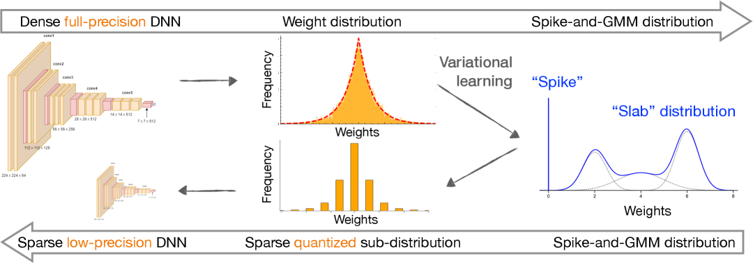
Figure 1: Our SQS method achieves high compression with minimal performance degradation by jointly pruning and quantizing model weights through variational learning. We employ a spike-and-GMM variational distribution to approximate full-precision weights: the spike component promotes sparsity for pruning, while the slab component (i.e., GMM) models a quantized weight distribution.

To tackle the above problem, we introduce a unified framework: Sparse Quantized Sub-distribution (SQS) compression method, which unifies pruning and quantization within a single variational learning process. Instead of applying pruning and quantization separately, the key idea of SQS is joint pruning and quantization that learns a sparse, quantized sub-distribution over network weights through variational learning. To model the variational posterior, we adopt a spike-and-slab prior combined with a Gaussian Mixture Model (GMM): the spike component encourages sparsity for pruning, while the GMM component models a quantized weight distribution, effectively mitigating performance degradation. The training pipeline of SQS is in Figure 1. Theoretically, we show that under mild conditions, our SQS method finds a sparse and quantized neural network that converges to the true underlying target neural network with high probability.

In our experiments, we compare several recent state-of-the-art compression methods across a range of widely used neural networks, including ResNet, BERT-base, LLaMA3, and Qwen2.5. Our findings show that (1) Under the same bit-width setting, our SQS achieves the highest compression rate, requiring fewer parameters than baselines. (2) At the same compression rate, our SQS achieves the smallest accuracy drop or F1 score drop among all approaches, with particularly strong performance at 2-bit and 4-bit precision.

Further ablation studies highlight the contributions of individual components: (1) The spike-and-slab distribution is more effective in promoting sparsity than Gaussian alternatives. (2) Bayesian averaging during inference outperforms greedy decoding. (3) An outlier-aware window strategy better preserves informative weight outliers compared to uniform windowing, further improving performance.

2 Preliminaries

Low-bit Quantization uses discrete low-bit values to approximate full-precision floating points, primarily to reduce precision for more efficient storage and computation while preserving essential information (Gholami et al., 2022). Formally, it is defined as a mapping $Q:\theta\in\mathbb{R}\rightarrow\mathcal{Q}=\{\mu_{1},\dots\mu_{K}\}$, where $\theta$ is the full-precision weight and $\mathcal{Q}$ denotes the set of low-bit discrete values. Representative quantization methods include deterministic quantization (Jacob et al., 2018), stochastic quantization (Courbariaux et al., 2015), and end-to-end learnable quantization (Dong et al., 2022).

Specifically, let $\theta=(\theta_{1},\ldots,\theta_{T})\in\mathbb{R}^{T}$ represent the full-precision weights of a deep neural network, with $\theta_{i}$ denoting the $i$-th weight. Given a quantization set $\mathcal{Q}=\{\mu_{1},\dots,\mu_{K}\}$, a general stochastic quantization is a mapping $Q:\theta\rightarrow\mathcal{Q}$, which is

$$Q(\theta_{i})=\mu_{k}, \qquad\text{with probability }p_{ki},$$

for $i=1,\dots,T$. Here $\mu_{k}$ is the learnable parameter and $p_{ki}$ is the corresponding probability for weight $\theta_{i}$ to be quantized to weights $\mu_{k}$. A key challenge is the distribution divergence between the quantized weights and the original weights, leading to significant performance degradation (Dong et al., 2022). To mitigate this, (Dong et al., 2022) propose to approximate the quantized weight distribution using a Gaussian Mixture Model (GMM):

$$Q(\theta_{i})\approx\sum_{k=1}^{K}\phi_{k}(\theta_{i};\pi_{k})\mathcal{N}(\mu_{k},\sigma^{2}_{k}),$$ (1)

where $\mathcal{N}(\mu_{k},\sigma_{k}^{2})$ denotes a Gaussian distribution, and $\phi_{k}(\theta_{i};\pi_{k})$ is the mixture weight for the Gaussian components $\mathcal{N}(\mu_{k},\sigma^{2}_{k})$. To control the sharpness of this mixture, a temperature-scaled softmax is applied to obtain $\phi_{k}(\theta_{i};\pi_{k})$, that is:

$$\phi_{k}(\theta_{i};\pi_{k})=\frac{\exp\left(\varphi_{k}(\theta_{i};\pi_{k})/\tau\right)}{\sum_{j=1}^{K}\exp\left(\varphi_{j}(\theta_{i};\pi_{j})/\tau\right)},$$ (2)

where the temperature parameter $\tau>0$ controls the concentration of the distribution. As $\tau\rightarrow 0$, the GMM in Equation (1) approaches a single dominant Gaussian component. Given a prior distribution $(\pi_{1},\dots,\pi_{K})$ over the quantization set $\mathcal{Q}$, the posterior component weight $\varphi_{k}(\theta_{i};\pi_{k})$ is:

$$\varphi_{k}(\theta_{i};\pi_{k})=\frac{\exp({\pi_{k}\mathcal{N}(\theta_{i}|\mu_{k},\sigma^{2}_{k})})}{\sum_{j=1}^{K}\exp({\pi_{j}\mathcal{N}(\theta_{i}|\mu_{j},\sigma^{2}_{j})})}.$$

Additionally, with sufficiently small $\sigma_{k}^{2}$, the GMM approximates a multinomial distribution over $\mathcal{Q}$, effectively bridging continuous and discrete quantization. For simplicity, we denote $\phi_{k}(\theta_{i})$ as a shorthand for $\phi_{k}(\theta_{i};\pi_{k})$ throughout the remainder of this paper.

In our experiments, we find that the GMM-based compression method (Dong et al., 2022) still cannot achieve a high compression rate while maintaining low-performance drop, as it cannot efficiently encourage sparsity during training.

Variational learning. Given an observed dataset $D$, the goal of a Bayesian framework is to infer the true posterior distribution $\pi(\mathbf{\theta}|D)\propto\pi(\mathbf{\theta})p(D;\mathbf{\theta})$, where $\pi(\mathbf{\theta})$ denotes the prior and $p(D;\mathbf{\theta})$ the likelihood. Since the posterior is generally intractable, variational learning (Jordan et al., 1999) is proposed to approximate it by selecting the closest distribution from a variational family $\mathcal{F}$ in terms of the Kullback–Leibler (KL) divergence (Csiszár, 1975):

$$q^{*}(\theta)\;=\;\operatorname*{arg\,min}_{q(\theta)\in\mathcal{F}}\,D_{\mathrm{KL}}\!\left(q(\theta)\,\|\,\pi(\theta\mid D)\right).$$ (3)

Following (Blei et al., 2017), this optimization is equivalent to minimizing the negative Evidence Lower Bound (ELBO), defined as:

$$\Omega(q):=-\mathbb{E}_{q(\theta)}[\log p(D;{\theta})]+D_{\mathrm{KL}}(q(\theta)\|\pi(\theta)),$$ (4)

where the first term measures how well the variational distribution $q(\theta)$ aligns with the log-likelihood of the observed data, and the second term regularizes $q(\theta)$ to stay close to the prior $\pi(\theta)$.

Our SQS method employs a variational family based on a spike-and-GMM distribution to approximate the sparse and quantized posterior. The first term in Equation (4) allows the spike-and-GMM to learn the posterior distribution given the data. For the second term, we adopt a slack-and-slab prior $\pi(\cdot)$ distribution to promote sparsity in the network weights.

3 Methodology

The objective is to approximate a full-precision neural network $f(\cdot;\theta)$ with a Bayesian model $f(\cdot;\tilde{\theta})$ that is both sparse and low-precision, while minimizing performance degradation. To achieve this, we employ a spike-and-slab distribution combined with a GMM to parameterize the variational posterior.

3.1 SQS: Variational learning for sparse and quantized sub-distribution

The spike-and-slab prior consists of a point mass at zero (spike) and a continuous distribution (slab) (Bai et al., 2020; Ishwaran and Rao, 2005). Formally, let $\gamma=(\gamma_{1},\ldots,\gamma_{T})$ be a binary indicator vector, where each $\gamma_{i}$ determines whether the corresponding weight $\theta_{i}$ is preserved ($\gamma_{i}=1$) or pruned ($\gamma_{i}=0$). The prior for each weight $\tilde{\theta}_{i}$ is defined as:

$$\tilde{\theta}_{i}\mid\gamma_{i}\sim\gamma_{i}\mathcal{N}(0,\sigma_{0}^{2})+(1-\gamma_{i})\delta_{0},\quad\gamma_{i}\sim\mathrm{Bern}(\lambda),$$

where $\lambda$ is the prior probability of retaining a weight, and $\sigma_{0}^{2}$ is the prior variance of the Gaussian slab. Marginalizing out the binary variable $\gamma_{i}$, the prior distribution over $\tilde{\theta}_{i}$ becomes:

$$\pi(\tilde{\theta}_{i})=\lambda\mathcal{N}(0,\sigma_{0}^{2})+(1-\lambda)\delta_{0},$$ (5)

where $1-\lambda$ corresponds to the prior pruning probability. For example, in a DNN with a target sparsity of $90\%$, setting $\lambda=0.1$ implies that each weight has a $90\%$ prior probability of being pruned.

To incorporate quantization into the variational family, we extend the spike-and-slab formulation by modeling the slab using a $K$-component GMM. Each variational distribution $q(\theta_{i})$ is then defined as:

$$\gamma_{i} \sim\mathtt{Bern}(\tilde{\lambda}_{i})$$

$$\tilde{\theta}_{i}|\gamma_{i} \sim\gamma_{i}\sum_{k=1}^{K}\phi_{k}(\theta_{i})\mathcal{N}(\mu_{k},\sigma^{2}_{k})+(1-\gamma_{i})\delta_{0}$$

where $\phi_{k}(\theta_{i})$ is the mixture weight for component $k$, and $\tilde{\lambda}_{i}$ is the variational probability of retaining weight $\theta_{i}$. The marginal variational distribution $q(\tilde{\theta}_{i})$ is:

$$q(\tilde{\theta}_{i})=\tilde{\lambda}_{i}\sum_{k=1}^{K}\phi_{k}(\theta_{i})\mathcal{N}(\mu_{k},\sigma^{2}_{k})+(1-\tilde{\lambda}_{i})\delta_{0}.$$ (6)

Given this variational family, we define the learning objective based on the ELBO:

$$\Omega(\tilde{\theta})=-\mathbb{E}_{q(\tilde{\theta})}\big[\log p(D;\tilde{\theta})\big]+\sum_{i=1}^{T}D_{\mathrm{KL}}\left(q(\tilde{\theta}_{i})\|\pi(\tilde{\theta}_{i})\right).$$ (7)

Yet, computing Equation (7) is intractable, as no closed-form solution exists for the KL divergence between $q(\tilde{\theta}_{i})$ and the spike-and-slab prior $\pi(\tilde{\theta}_{i})$. To overcome this challenge, we propose the following approximation:

$$\Omega_{\mathtt{apx}}(\tilde{\theta})= \log{p\left(D;\tilde{\lambda}_{i}\sum_{k=1}^{K}\mu_{k}\phi_{k}(\theta_{i})\right)}$$

$$+\sum_{i=1}^{T}D_{\mathrm{KL}}(\mathtt{Bern}(\tilde{\lambda}_{i})\|\mathtt{Bern}(\lambda_{i}))$$

$$+\sum_{i=1}^{T}\tilde{\lambda}_{i}D_{\mathrm{KL}}(\mathcal{N}(\mu_{k^{*}},\sigma^{2}_{k^{*}})\|\mathcal{N}(0,\sigma^{2}_{0})),$$ (8)

where $k^{*}=\operatorname*{arg\,max}_{1\leq k\leq K}\phi_{k}(\theta_{i})$. The first term is an approximation of the $\mathbb{E}_{q(\tilde{\theta})}[\log p(D;\tilde{\theta})]$ in Equation (7) by replacing $q(\tilde{\theta})$ with the Delta measure at the mean $\mathbb{E}[\tilde{\theta}]=\tilde{\lambda}_{i}\sum_{k=1}^{K}\mu_{k}\phi_{k}(\theta_{i};\pi,\tau)$. The second and the third terms provide an upper bound of the term $\sum_{i=1}^{T}D_{\mathrm{KL}}\left(q(\tilde{\theta}_{i})\|\pi(\tilde{\theta}_{i})\right)$ by applying Lemma 2. A detailed derivation of Equation (8) is in Appendix A.

Inference. In the inference stage, we first sample the sparse and quantized weight given the learned parameters and predict the output $\widehat{y}$ for each testing input $x$. Let $\widehat{q}(\cdot)$ denote the optimization solution of the above variational learning, associated with the optimal parameter estimations $\{\hat{\theta}_{i},\hat{\mu}_{i},\hat{\sigma}^{2}_{i},\hat{\lambda}_{i}\}_{i=1}^{T}$, and the corresponding $\widehat{\phi}_{k}$’s (for each $\hat{\theta}_{i}$) are obtained from Equation (2). Then the $i$-th quantized weight $\theta_{i}$ are sampled from the quantization function:

$$Q(\tilde{\theta}_{i})=\hat{\mu}_{k} \qquad\text{with probability }\widehat{\phi}_{k}(\hat{\theta}_{i})$$ (9)

Compared to sampling from $\mathcal{N}(\hat{\mu}_{k},\hat{\sigma}^{2}_{k})$, posterior sampling in Equation (9) reduces memory consumption.

To enforce sparsity, we introduce a user-specified pruning parameter, the Non-zero rate. Each weight ($\theta_{i}$) is associated with a score ($\hat{\lambda}_{i}$), which reflects the likelihood of being retained. We deterministically prune by setting the (i)-th weight to zero if ($\hat{\lambda}_{i}$) is smaller than the Non-zero-quantile of all ($\hat{\lambda}_{i}$) values; otherwise, the weight is kept unchanged. Formally,

$$\theta_{i}=\begin{cases}0,&\text{if }\hat{\lambda}_{i}<\texttt{Non-zero}\text{ quantile of all }\hat{\lambda}_{i},\\ \theta_{i},&\text{otherwise}.\end{cases}$$

This deterministic rule provides exact control over the sparsity level, in contrast to stochastic pruning via posterior sampling (Bai et al., 2020; Sun et al., 2022), which does not guarantee a fixed sparsity rate and often requires an additional pruning step.

Bayesian averaging. Given a test input $x$, the predicted output $\widehat{y}$ is computed using Bayesian averaging:

$$\widehat{y}=\frac{1}{M}\sum_{m=1}^{M}f(x;\tilde{\theta}^{m})$$ (10)

where $\tilde{\theta}^{m}$’s are $M$ many samples from the sparse quantized sub-distribution. Our ablation study (Figure 3) shows that Bayesian averaging consistently yields smaller accuracy degradation than the greedy alternative (Equation 34, Appendix C).

Outlier-aware windowing. Recent studies show that the weight distribution of large language models (LLMs) often contains significant outliers (Wei et al., 2022). To address this, we use an outlier-aware windowing strategy to enhance the performance of SQS. Specifically, the full-precision weights are partitioned into four groups using window sizes determined by a modified $1.5\times$Interquartile Range (IQR) rule (Dekking, 2005), which helps preserve large-magnitude weights during quantization. Each group is then quantized to $K$ representative values. As shown in the ablation study (Figure 2), this strategy outperforms the approach using equal-sized windows. Implementation details are provided in Appendix C, and the full procedure is summarized in Algorithm 1 in the Appendix.

Remarks. DGMS (Dong et al., 2022) adopts a mixture of Gaussians, but uses it primarily as a clustering mechanism. In contrast, our method leverages a principled Bayesian framework that supports posterior inference and enables Bayesian model averaging, enhancing robustness to quantization noise. Furthermore, by unifying pruning and quantization within a spike-and-GMM variational family, our approach creates a joint optimization space that encourages globally optimal solutions across both pruning and quantization.

3.2 Theoretical Justification of SQS method

For clarity, this section focuses on regression tasks with fully connected neural networks and shows that the variational posterior of sparse and quantized neural networks, i.e., the optimization of Equation (7). We show that this variational posterior converges to a true regression function under some mild conditions.

Consider a regression problem with random covariates,

$$Y_{i}=f_{0}(X_{i})+\varepsilon_{i},\quad\text{ for }i=1,\ldots,n,$$ (11)

where $f_{0}:[0,1]^{p}\rightarrow\mathbb{R}$ is the underlying unknown true function, $X_{i}\sim\mathcal{U}([0,1]^{p})$ sample from $p$-dimensional uniform distribution, $\epsilon_{i}\overset{iid}{\sim}\mathcal{N}(0,\sigma^{2}_{\epsilon})$ is the noise term from Gaussian distribution of zero mean and variance $\sigma^{2}_{\epsilon}$. Let $P_{0}$ denote the true underlying probability measure of the data, and $p_{0}$ denote the corresponding density function. A $L$-hidden layer fully connected NNs with constant layer width $N$ and parameters $W_{i}\in\mathbb{R}^{N\times N}$, $b_{i}\in\mathbb{R}^{N}$ and activation function $\sigma(\cdot)$ can be defined as:

$$f_{\theta}(X)=W_{L+1}\sigma_{b_{L}}(W_{L}\sigma_{b_{L-1}}\ldots\sigma_{b_{1}}(W_{1}X))+b_{L+1}.$$ (12)

For simplicity, $\sigma_{\epsilon}$ is assumed to be known. Let $s^{*}$ be the “oracle” sparsity level (see Equation 16 in Appendix B for formal definition) and $H(T,s,K)$ be the set of network weight parameters such that the network has a sparsity of $s$ and shares at most $K$ distinct values. Let $P_{0}$ and $P_{\theta}$ be the true data distribution and the distribution under parameter $\theta$, respectively.

Theorem 1.

Let $r_{n}^{*}=\left((L+1)s^{*}/n\right)\log N+(s^{*}/n\log(p\sqrt{n/s^{*}}))$, $\varepsilon_{n}^{*}=\sqrt{r_{n}^{*}}\log^{\delta}(n)$ for any $\delta>1$, and $\xi_{n}^{*}=\inf_{\theta\in H(T,s,K),\left\|\theta\right\|\leq B}\left\|f_{\theta}-f_{0}\right\|_{\infty}^{2}$. Then, under mild conditions specified in the supplementary material, with high probability:

$$\int_{\mathbb{R}^{T}}d^{2}(P_{\theta},P_{0})\widehat{q}(\theta)d\theta\leq C\varepsilon_{n}^{*2}+C^{\prime}(r_{n}^{*}+\xi_{n}^{*}),$$ (13)

where $d(\cdot,\cdot)$ denotes the Hellinger distance, and $C$ and $C^{\prime}$ are some constants.

Sketch of Proof.

Based on prior work (Bai et al., 2020), the proof proceeds in two steps. Lemma 4 establishes a high-probability bound on the ELBO in Equation (7). Lemma 5 connects this bound to the convergence of the variational distribution toward the true full-precision posterior. Together, these results show that the variational posterior induced by our method converges to the true regression function with high probability. The full proof is in Appendix B. ∎

Remark. Similar to previous Bayesian sparse DNN results (Bai et al., 2020; Chérief-Abdellatif, 2020), the convergence rate of variational Bayes is determined by the deep neural network structure via 1) statistical estimation error $\varepsilon_{n}^{*}$, 2) variational error $r_{n}^{*}$, and 3) approximation error $\xi_{n}^{*}$. The first two positively relate to the network capacity, while the third one negatively relates to the network capacity. The estimation error $\varepsilon_{n}^{*}$ and variational error $r_{n}^{*}$ vanish as $n\to\infty$. Prior work (Beknazaryan, 2022) shows that under $B\geq 2$, $K\geq 6$, and $\beta$-Hölder smoothness of $f_{0}$, the approximation error $\xi_{n}^{*}$ also vanishes.

While the theoretical analysis mainly considers an $L$-hidden layer fully connected NN with constant layer width $N$, our method $SQS$ is empirically validated on a variety of models such as ResNets, BERT-based models, and LLMs (refer to Section 5).

4 Related Works

Weight pruning was initially introduced by (LeCun et al., 1989), with further development by (Hassibi et al., 1993) through a mathematical method known as the Optimal Brain Surgeon (OBS). This approach selects weights for removal from a trained neural network using second-order information. Subsequent improvements, as indicated by studies (Dong et al., 2017; Wang et al., 2019; Singh and Alistarh, 2020), have adapted OBS for large-scale DNNs by employing numerical techniques to estimate the second-order information required by OBS. Meanwhile, (Louizos et al., 2018) has introduced an $L_{0}$-regularized method to promote sparsity in DNNs. (Frankle and Carbin, 2019) established a critical insight that within a randomly initialized DNN, an optimal sub-network can be identified and extracted. Recently, (Xia et al., 2024) showed that structured pruning combined with targeted retraining can significantly reduce computational costs while preserving robust performance for large language models. Concurrently, spike-and-slab distributions have been employed to promote sparsity in DNNs using Bayesian Neural Networks formulation (Deng et al., 2019; Blundell et al., 2015; Bai et al., 2020).

Low-bit quantization. Quantization improves DNN efficiency, particularly in resource-constrained environments (Sze et al., 2017; Frantar et al., 2023; Lin et al., 2024, 2025). Research in this field typically follows two paradigms: discontinuous-mapping and continuous-mapping quantization. Discontinuous-mapping methods project full-precision weights onto a low-bit grid using rounding operations (Gupta et al., 2015; Hubara et al., 2018; Wu et al., 2018; Louizos et al., 2019; Courbariaux et al., 2015; De Sa et al., 2018; Marchesi et al., 1993). The non-differentiability of these mappings necessitates the use of the straight-through estimator (STE) for gradient approximation (Courbariaux and Bengio, 2016; Rastegari et al., 2016). However, STE-based training may introduce pseudo-gradients, leading to training instability (Yin et al., 2019). Meanwhile, many researchers propose post-training quantization methods that have limited access to the training dataset (Wang et al., 2020a; Hubara et al., 2021; Li et al., 2021; Frantar and Alistarh, 2022; Frantar et al., 2023; Lin et al., 2024).

Table 1: For compressing ResNet models, we benchmark all methods evaluated on the CIFAR-10 dataset. Using ResNet-32 and ResNet-56 models, our SQS consistently achieves higher compression rates with smaller Top-1 Accuracy drops compared to all baselines.

ResNet-20	Methods	Comp.	Bits	Non-zero	Compression	Top-1 Accuracy
		type		rate (%)	rate	drop
	LQNets (Zhang et al., 2018)	Q	$2$	$100\%$	$16\times$	$1.20\%$
	DGMS (Dong et al., 2022)	P+Q	$2$	$56\%$	$29\times$	$\mathbf{0.87\%}$
	SQS (Ours)	P+Q	$2$	$\mathbf{50\%}$	$\mathbf{32\times}$	$1.47\%$
(a) Compressing 32Bits ResNet-20 model on CIFAR-10 dataset with Top-1 Accuracy $92.60\%$.
ResNet-32	Methods	Comp.	Bits	Non-zero	Compression	Top-1 Accuracy
		type		rate (%)	rate	drop
	TTQ (Zhu et al., 2017)	Q	$2$	$100\%$	$16\times$	$1.90\%$
	DGMS (Dong et al., 2022)	P+Q	$2$	$59\%$	$27\times$	$1.30\%$
	SQS (Ours)	P+Q	$2$	$\mathbf{50\%}$	32$\times$	$\mathbf{1.29\%}$
(b) Compressing 32Bits ResNet-32 model on CIFAR-10 dataset with Top-1 Accuracy $93.53\%$.
ResNet-56	Methods	Comp.	Bits	Non-zero	Compression	Top-1 Accuracy
		type		rate (%)	rate	drop
	TTQ (Zhu et al., 2017)	Q	2	$100\%$	16$\times$	$1.06\%$
	L1 (Li et al., 2017)	P	32	$10\%$	10$\times$	$1.83\%$
	DGMS (Dong et al., 2022)	P+Q	$2$	$52\%$	$31\times$	$0.89\%$
	SQS (Ours)	P+Q	2	$\mathbf{50\%}$	$\mathbf{32\times}$	$\mathbf{0.84\%}$
(c) Compressing 32Bits ResNet-56 model on CIFAR-10 dataset with Top-1 Accuracy $94.37\%$.

Continuous-mapping quantization offers an alternative that avoids pseudo-gradients, leading to more stable training (Yin et al., 2019; Nielsen et al., 2025). These methods often use variational learning (Ullrich et al., 2017; Louizos et al., 2017; Shayer et al., 2018) or Markov Chain Monte Carlo techniques (Roth and Pernkopf, 2018) to approximate discrete weight distributions. However, variational methods often require manual prior specification (Ullrich et al., 2017; Louizos et al., 2017; Shayer et al., 2018), while MCMC approaches can be memory-intensive (Roth and Pernkopf, 2018). DGMS (Dong et al., 2022) addresses these limitations through automated quantization using GMMs. Our work extends DGMS by integrating pruning and quantization into a unified framework, thereby achieving higher compression rates.

5 Experiments

In this section, we show that our SQS achieves a much higher compression rate (see the second-to-last column in Tables 1-3) while incurring a comparable or smaller performance drop (see the last column in the same tables). Through ablation studies, we further validate that (1) under the same sparsity level, the spike-and-slab prior more effectively preserves model accuracy (see Table 4). (2) Under identical hyperparameter settings, we show that SQS with Bayesian averaging is better than using the greedy approach (see Figure 3).

5.1 Experiment settings

We evaluate all methods using two metrics: the compression rate and the performance drop (i.e., Accuracy drop or F1 score drop). The compression rate is defined as the memory footprint of the compressed over the original dense full-precision model:

$$\text{Compression rate}=\frac{32}{\texttt{Bits}}\times\frac{1}{\texttt{Non-zero}},$$ (14)

where Bits indicates the number of low-precision bits needed to represent the model, for SQS the Bits is equal to $\log_{2}(K)$. Non-zero is the proportion of non-zero weights over the total weights. In all our experiments, the Non-zero is configured as a hyperparameter to control the sparsity.

To ensure fair comparison, each method is initialized with the same full-precision pre-trained model and is run with the same set of hyperparameters for compression. All methods are constrained to a maximum runtime of 24 hours. The resulting compressed models are then evaluated on the same test sets, and the key performance metrics are summarized in the corresponding tables.

We compare methods of different compression types (the “Comp. type” column): “P+Q” denotes combined pruning and quantization, “P” denotes pruning only, and “Q” denotes quantization only. Appendix D provides detailed experimental configurations and baseline settings.

Table 2: Compressing 32Bits Bert-base model on SQuADv1.1 dataset with F1 score $88.68\%$. Our SQS achieves higher compression rates with smaller F1 score drops compared to all baselines.

BERT-base	Methods	Comp.	Bits	Non-zero	Compression	F1 score
		type		rate (%)	rate	drop
	GMP (Zhu and Gupta, 2017)	P	$32$	$50\%$	$2\times$	$22.89$
	L-OBS (Dong et al., 2017)	P	$32$	$50\%$	$2\times$	$10.86$
	ExactOBS (Frantar and Alistarh, 2022)	P	$32$	$25\%$	$4\times$	$6.43$
	PLATON (Zhang et al., 2022)	P	$32$	$20\%$	$5\times$	$2.20$
	OBQ (Frantar and Alistarh, 2022)	Q	$3$	$100\%$	$11\times$	$3.24$
	GPTQ (Frantar et al., 2023)	Q	$3$	$100\%$	$11\times$	$2.51$
	OBC (Frantar and Alistarh, 2022)	P+Q	$4$	$50\%$	$16\times$	$2.33$
	SQS (Ours)	P+Q	4	$\mathbf{25\%}$	$\mathbf{32\times}$	$\mathbf{1.66}$

Table 3: Compression results for LLAMA3.2 and Qwen2.5 models on the SST-2 dataset. Our SQS achieves significantly higher compression rates than AWQ while maintaining comparable ($\leq 3\%$) performance drops.

Llama3.2	Methods	Comp.	Bits	Non-zero	Compression	Top-1 accuracy
		type		rate (%)	rate	drop
	AWQ (Lin et al., 2024)	P	$4$	$100\%$	$8\times$	$\mathbf{0.46\%}$
	DGMS (Dong et al., 2022)	P+Q	$6$	$82\%$	$7\times$	$46.67\%$
	SQS (Ours)	P+Q	$6$	$\mathbf{25\%}$	$\mathbf{21\times}$	$1.48\%$
(a) Compressing 32Bits Llama3.2-1B model on SST-2 dataset with Top-1 Accuracy $94.72\%$.
Qwen2.5	Methods	Comp.	Bits	Non-zero	Compression	Top-1 accuracy
		type		rate (%)	rate	drop
	AWQ (Lin et al., 2024)	P	4	100%	$8\times$	$\mathbf{1.54\%}$
	DGMS (Dong et al., 2022)	P+Q	$6$	$\mathbf{34\%}$	$\mathbf{16}\times$	$50.80\%$
	SQS (Ours)	P+Q	$6$	$50\%$	${11\times}$	$2.46\%$
(b) Compressing 32Bits Qwen2.5-0.5B model on SST-2 dataset with Top-1 Accuracy $92.60\%$.

5.2 Experimental analysis

Compression on ResNet models. Table 1 summarizes the result of all methods for compressing ReNet-18, ReNet-32 and ReNet-56, evaluated on the CIFAR-10 dataset. On compressing the ResNet-18 model, our SQS attains a better compression rate than the baselines. On compressing ResNet-32 and ResNet-56 models, our SQS attains substantially higher compression rates while incurring smaller accuracy drops compared to the baselines. Optimizing pruning and quantization separately overlooks redundancies in each step; by merging them into a single optimization, we effectively eliminate these inefficiencies

Compression on BERT-base model. We apply our compression method to the BERT-base model (Devlin et al., 2019) and evaluate its performance on the SQuAD v1.1 dataset (Rajpurkar et al., 2016). The evaluation metrics include the F1 score drop and the compression rate. As shown in Table 2, our method achieves the lowest F1 score drop and the highest compression rate, outperforming existing methods. This demonstrates the effectiveness of our SQS method in preserving accuracy under aggressive compression.

Compression on Llama and Qwen models. In Table 3, we compare our method SQS with others on the SST2 task in the GLUE benchmark using Llama3.2-1B and Qwen2.5-0.5B models, as our method could preserve the weights outliers, which are crucial in maintaining the performance (Lin et al., 2024). We further observe a big performance drop of the DGMS (Dong et al., 2022) method for compressing Llama3.2-1B and Qwen2.5-0.5B, which occurs because the attention weights distribution is not Gaussian (see Figure 2(left)), and it fails to capture large magnitude weights. Furthermore, DGMS doesn’t allow customization of the sparsity level, thus it presents an unreasonable performance drop.

Table 4: Impact of the Gaussian prior and the spike-and-slab prior, for compressing a 32 bits ResNet-18 model on the CIFAR-100 dataset with Top-1 Accuracy $79.26\%$. The spike-and-slab prior used in our SQS consistently yields better performance than the Gaussian prior across all sparsity-level settings.

ResNet-18	Bits	Non-zero (%)	Compression rate	Top-1 Accuracy drop
				Gaussian prior	Spike-and-slab prior (Ours)
	$4$	$50\%$	$16\times$	$4.51\%$	$\mathbf{3.12}\%$
	$4$	$40\%$	$20\times$	$5.60\%$	$\mathbf{3.21}\%$
	$4$	$30\%$	$27\times$	$11.42\%$	$\mathbf{5.54}\%$
	$4$	$20\%$	$40\times$	$44.04\%$	$\mathbf{5.59}\%$

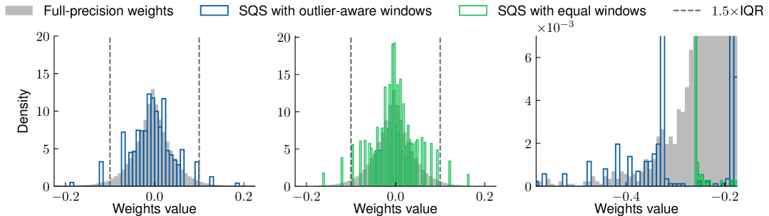
Figure 2: Impact of different window strategies. For the compressed weight distributions in the first attention layer of the Llama3.2-1B model, SQS with outlier-aware window strategy (left) yields better preservation of the full-precision weight distribution compared to the equal-sized window (middle). This advantage is also evident in the left tail region shown in (right). Weight visualization of layers of Llama3.2-1B and Qwen2.5 is provided in the Appendix E.

5.3 Ablation studies for SQS method

Impact of different priors. We evaluate the impact of the choices of prior—specifically, the Gaussian prior vs. the spike-and-slab prior—on model performance. Please see Appendix D.2 for detailed setup on the Gaussian prior. The task involves compressing a ResNet-18 model at varying sparsity levels by representing each layer’s weights using $K=16$ components and evaluating performance on the CIFAR-100 dataset. In Table 4, the spike-and-slab prior consistently outperforms the Gaussian prior across all sparsity levels. Notably, the Gaussian prior leads to significantly degraded performance under high sparsity, suggesting its limitation in inducing effective posterior sparsity in DNN weights.

Impact of different window strategies. We use the first attention layer weights in the Llama3.2-1B model as the case study. The full-precision weights exhibit a long-tail distribution, where a fraction of weights have large magnitudes. Based on this observation, we further introduce an outlier-aware window strategy to fit the full-precision weights distribution. As shown in Figure 2 (left) and (middle), the quantized weight generated from SQS with the outlier-aware window strategy matches the distribution better than using the equal window strategy. In Figure 2 (right), The SQS with an outlier-aware window strategy matches the distribution at the tails better than using the equal window strategy. More results on the rest of the layers’ weight distribution are provided in the Appendix E.

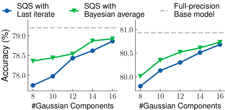
Figure 3: Comparison of inference accuracy on the CIFAR-100 dataset using ResNet-18 (left) and ResNet-50 (right). Under the same number of Gaussian components, SQS with Bayesian averaging (in Equation 10) results in a smaller accuracy drop compared to using a greedy approach (in Equation 34).

Impact of different inference strategies. We evaluate the effectiveness of two inference strategies—Bayesian averaging and greedy approach, as defined in Equation (10)—within our SQS framework. To ensure a fair comparison, we assess the performance of compressing ResNet-18 and ResNet-50 models while varying the number of Gaussian components. The sparsity level is fixed to zero (i.e., no pruning), so that all performance degradation arises purely from quantization. As shown in Figure 3, using fewer components results in a larger accuracy drop. Under the same number of components, SQS with Bayesian averaging consistently achieves a smaller accuracy drop compared to the greedy approach strategy.

6 Conclusion

In this paper, we proposed a unified framework for compressing full-precision DNNs by combining pruning and quantization into one integrated optimization process through variational learning. Unlike conventional approaches that apply pruning and quantization sequentially—often resulting in suboptimal solutions—our method jointly explores a broader solution space, achieving significantly higher compression rates with comparable performance degradation. To address the intractability of the original objective, we introduce an efficient approximation that enables scalable optimization. We evaluate our method across a range of benchmarks, including ResNets, BERT-base, Llama3, and Qwen2.5.

Experimental results demonstrate that our approach consistently outperforms existing baselines in compression rate while maintaining competitive accuracy, highlighting its potential for efficient deployment in resource-constrained environments.

Contents

Appendix A Derivation of Approximate Objective

A.1 An upper bound on the KL divergence between two mixtures

To simplify the ELBO and validate our approach, we reformulate a key lemma from previous work (Chérief-Abdellatif and Alquier, 2018, Lemma 6.1). It is a tool widely used in signal processing (Hershey and Olsen, 2007). We provide the proof for the sake of completeness.

Lemma 2 (From Lemma 6.1 in (Chérief-Abdellatif and Alquier, 2018) ).

For any $K>0$, the KL divergence between any two mixture densities $\sum_{k=1}^{K}w_{k}g_{k}$ and $\sum_{k=1}^{K}\tilde{w}_{k}\tilde{g}_{k}$ is upper bounded by

$$D_{\mathrm{KL}}\left(\sum_{k=1}^{K}w_{k}g_{k}\Big\|\sum_{k=1}^{K}\tilde{w}_{k}\tilde{g}_{k}\right)\leq\sum^{K}_{k=1}w_{k}D_{\mathrm{KL}}(g_{k}\|\tilde{g}_{k})+\sum_{k=1}^{K}w_{k}\log\left(\frac{w_{k}}{\tilde{w}_{k}}\right)$$

Proof.

We expand the KL divergence term by its definition, thus it could have the following:

$$D_{\mathrm{KL}}\left(\sum_{k=1}^{K}w_{k}g_{k}\Big\|\sum_{k=1}^{K}\tilde{w}_{k}\tilde{g}_{k}\right) =\int\left(\sum_{k=1}^{K}w_{k}g_{k}\right)\log\left(\frac{\sum_{k=1}^{K}w_{k}g_{k}}{\sum_{k=1}^{K}\tilde{w}_{k}\tilde{g}_{k}}\right)$$

$$\leq\int\sum_{k=1}^{K}w_{k}g_{k}\log\left(\frac{w_{k}g_{k}}{\tilde{w}_{k}\tilde{g}_{k}}\right)$$

$$=\int\sum_{k=1}^{K}w_{k}g_{k}\log\left(\frac{g_{k}}{\tilde{g}_{k}}\right)+\int\sum_{k=1}^{K}w_{k}g_{k}\log\left(\frac{w_{k}}{\tilde{w}_{k}}\right)$$

$$=\sum_{k=1}^{K}w_{k}\int g_{k}\log\left(\frac{g_{k}}{\tilde{g}_{k}}\right)+\sum_{k=1}^{K}w_{k}\log\left(\frac{w_{k}}{\tilde{w}_{k}}\right)\left(\int g_{k}\right)$$

$$=\sum^{K}_{k=1}w_{k}D_{\mathrm{KL}}(g_{k}\|\tilde{g}_{k})+\sum_{k=1}^{K}w_{k}\log\left(\frac{w_{k}}{\tilde{w}_{k}}\right),$$

where the first inequality is due to the Jensen inequality and the convexity of the function $x\log(x)$. This completes the proof. ∎

A.2 Derivation of Approximate Objective

We aim to approximate the ELBO objective:

$$\Omega(\tilde{\theta})=-\underbrace{\mathbb{E}_{q(\tilde{\theta})}[\log p(D;\tilde{\theta})]}_{\mathtt{Part\;1}}+\sum_{i=1}^{T}D_{\mathrm{KL}}\left(q(\tilde{\theta}_{i})\|\pi(\tilde{\theta}_{i})\right).$$ (15)

where $\pi(\tilde{\theta}_{i})$ is defined in Equation (5) and $q(\tilde{\theta}_{i})$ is defined in Equation (6):

$$q(\tilde{\theta}_{i}) =\tilde{\lambda}_{i}\sum_{k=1}^{K}\phi_{k}(\theta_{i})\mathcal{N}(\mu_{k},\sigma_{k}^{2})+(1-\tilde{\lambda}_{i})\delta_{0},$$

$$\pi(\tilde{\theta}_{i}) =\lambda\mathcal{N}(0,\sigma_{0}^{2})+(1-\lambda)\delta_{0}.$$

It is important to note that the KL divergence between the variational distribution and the spike-and-slab prior distribution does not have a closed-form solution.

Step 1: Approximate the expected log-likelihood.

The first term $\mathbb{E}_{q(\tilde{\theta})}[\log p(D;\tilde{\theta})]$ can be expensive to compute, due to the sampling over spike-and-slab distribution. A tractable approximation is to replace the expectation with the log-likelihood at the mean parameter: $\mathbb{E}_{q(\tilde{\theta})}[\log p(D;\tilde{\theta})]\approx\log p(D;\mathbb{E}_{q(\tilde{\theta})}[\tilde{\theta}])$. Since,

$$\mathbb{E}_{q(\tilde{\theta})}[\tilde{\theta}]=\tilde{\lambda}_{i}\sum_{k=1}^{K}\mu_{k}\phi_{k}(\theta_{i})+(1-\tilde{\lambda}_{i})*0=\tilde{\lambda}_{i}\sum_{k=1}^{K}\mu_{k}\phi_{k}(\theta_{i}),$$

We then have:

$$\mathtt{Part\;1}\approx\log{p\left(D;\tilde{\lambda}_{i}\sum_{k=1}^{K}\mu_{k}\phi_{k}(\theta_{i})\right)}.$$

Step 2: Upper Bound KL between spike-and-slab distributions.

The KL divergence between the marginal variational posterior and the prior is intractable due to the presence of both the Dirac delta and the mixture components. To upper-bound the KL divergence between them, we apply Lemma 2 by matching component structure:

$$D_{\mathrm{KL}}(q\|\pi) \leq\sum_{j=1}^{2}w_{j}D_{\mathrm{KL}}(g_{j}\|\tilde{g}_{j})+\sum_{j=1}^{2}w_{j}\log\left(\frac{w_{j}}{\tilde{w}_{j}}\right),$$

with $$w_{1}=\tilde{\lambda}_{i},g_{1}=\sum_{k=1}^{K}\phi_{k}(\theta_{i})\mathcal{N}(\mu_{k},\sigma_{k}^{2}),\tilde{w}_{1}=\lambda,\tilde{g}_{1}=\mathcal{N}(0,\sigma_{0}^{2})$$

$$w_{2}=1-\tilde{\lambda}_{i},g_{2}=\delta_{0},\tilde{w}_{2}=1-\lambda,\tilde{g}_{2}=\delta_{0}$$

Substituting into the bound, we obtain:

$$D_{\mathrm{KL}}(q(\tilde{\theta}_{i})\|\pi(\tilde{\theta}_{i}))\leq \tilde{\lambda}_{i}D_{\mathrm{KL}}\left(\sum_{k=1}^{K}\phi_{k}(\theta_{i})\mathcal{N}(\mu_{k},\sigma_{k}^{2})\Big\|\mathcal{N}(0,\sigma_{0}^{2})\right)+(1-\tilde{\lambda}_{i})\underbrace{D_{\mathrm{KL}}(\delta_{0}\|\delta_{0})}_{=0}$$

$$+\tilde{\lambda}_{i}\log\frac{\tilde{\lambda}_{i}}{\lambda}+(1-\tilde{\lambda}_{i})\log\frac{1-\tilde{\lambda}_{i}}{1-\lambda}.$$

Combining the terms, we have:

$$D_{\mathrm{KL}}(q(\tilde{\theta}_{i})\|\pi(\tilde{\theta}_{i}))\leq\tilde{\lambda}_{i}D_{\mathrm{KL}}\left(\sum_{k=1}^{K}\phi_{k}(\theta_{i})\mathcal{N}(\mu_{k},\sigma^{2}_{k})\Big\|\mathcal{N}(0,\sigma_{0}^{2})\right)+D_{\mathrm{KL}}(\mathrm{Bern}(\tilde{\lambda}_{i})\|\mathrm{Bern}(\lambda)),$$

Note that the first term on the right-hand side, which is the KL divergence between the GMM and the Gaussian distribution, does not have a closed form. But it can be further upper-bounded as:

$$D_{\mathrm{KL}} \left(\sum_{k=1}^{K}\phi_{k}(\theta_{i})\mathcal{N}(\mu_{k},\sigma^{2}_{k})\Big\|\mathcal{N}(0,\sigma^{2}_{0})\right)=D_{\mathrm{KL}}\left(\sum_{k=1}^{K}\phi_{k}(\theta_{i})\mathcal{N}(\mu_{k},\sigma^{2}_{k})\Big\|\sum_{k=1}^{K}\phi_{k}(\theta_{i})\mathcal{N}(0,\sigma^{2}_{0})\right)$$

$$\leq \sum_{k=1}^{K}\phi_{k}(\theta_{i})D_{\mathrm{KL}}\left(\mathcal{N}(\mu_{k},\sigma^{2}_{k})\|\mathcal{N}(0,\sigma^{2}_{0})\right)+\sum_{k=1}^{K}\phi_{k}(\theta_{i})\underbrace{\log\left(\frac{\phi_{k}(\theta_{i})}{\phi_{k}(\theta_{i})}\right)}_{=0}$$

$$= \underbrace{\sum_{k=1}^{K}\phi_{k}(\theta_{i})D_{\mathrm{KL}}\left(\mathcal{N}(\mu_{k},\sigma^{2}_{k})\|\mathcal{N}(0,\sigma^{2}_{0})\right)}_{\mathtt{Part\penalty 10000\ 2}},$$

where the inequality is obtained by Lemma 2. Empirically, we approximate the mixture KL by evaluating only the dominant component:

$$\mathtt{Part\;2}\approx D_{\mathrm{KL}}(\mathcal{N}(\mu_{k^{*}},\sigma^{2}_{k^{*}})\|\mathcal{N}(0,\sigma^{2}_{0})),\qquad\text{where }k^{*}=\operatorname*{arg\,max}_{k}\phi_{k}(\theta_{i})$$

where we approximate the inner sum over $k$ using the maximum-weight component, which is the $k^{*}$-th component.

As a small temperature is needed to avoid a flat posterior distribution, which could introduce large differences between the training phase and inference phase.

Finally, putting all approximations together, we obtain:

$$\Omega_{\mathtt{apx}}(\tilde{\theta})= -\log{p\left(D;\tilde{\lambda}_{i}\sum_{k=1}^{K}\mu_{k}\phi_{k}(\theta_{i};\pi,\tau)\right)}$$

$$+\sum_{i=1}^{T}D_{\mathrm{KL}}(\mathrm{Bern}(\tilde{\lambda}_{i})\|\mathrm{Bern}(\lambda))$$

$$+\sum_{i=1}^{T}\tilde{\lambda}_{i}D_{\mathrm{KL}}(\mathcal{N}(\mu_{k^{*}},\sigma^{2}_{k^{*}})\|\mathcal{N}(0,\sigma^{2}_{0})),\qquad\text{where }k^{*}=\operatorname*{arg\,max}_{1\leq k\leq K}\phi_{k}(\theta_{i}).$$

which is the result shown in Equation (8).

Appendix B Proof of Theorem 1

Consider a $L$-hidden layer fully connected neural network with the ReLU activation function $\sigma_{b}:\mathbb{R}^{d}\rightarrow\mathbb{R}^{d}$ defined as $\sigma_{b}(X)=\max\{0,X-b\}$ on some dimension $d$ and parameter $b$. The number of neurons in each layer is defined as $p_{i}$ for $i=1,\dots,L$. The weights and biases are denoted as the $W_{i}\in\mathbb{R}^{N\times N}$ and $b_{i}\in\mathbb{R}^{N}$. Thus given the parameters $\mathbf{p}=(p_{1},\cdots,p_{L})$ and let $\theta$ denote the vector obtained by stacking all entries of the weight matrices $W_{i}$ and bias vectors $b_{i}$, then the fully connected network can be presented as:

$$f_{\theta}(X)=W_{L+1}\sigma_{b_{L}}(W_{L}\sigma_{b_{L-1}}\ldots\sigma_{b_{1}}(W_{1}X))+b_{L+1}.$$

The DNN $f_{\theta}$ also introduces a probability measure of the data, which we denote as $P_{\theta}$, and $p_{\theta}$ is the corresponding density function, $p_{\theta}(D)$ would be the likelihood of the data $D$.

One can define the sparse parameter space with sparsity parameter $s$ as $\{\theta\in\mathbb{R}:\left\|\theta\right\|_{0}<s\}$, where $\theta$ has only $s$ many non-zero entries. Then we can further introduce the sparse and quantized weights space $H(T,s,K)$ as follows:

$$\mathcal{I}(T,s,K) =\{I=[r_{1},\dots,r_{T}]^{\top}|\left\|I\right\|_{0}\leq s,r_{i}\in\{0,1\}^{K},\left\|r_{i}\right\|_{0}\leq 1\},$$

$$H(T,s,K) =\left\{\theta\in\mathbb{R}^{T}|\theta=I\cdot E,E\in[-B,B]^{K},I\in\mathcal{I}(T,s,K)\right\},$$

where $B$ is some constant satisfies $B>2$ and $\mathcal{I}(T,s,K)$ is the indexing space, each element $I\in\mathcal{I}(T,s,K)$ consists of $s$ many $K$-dimension one-hot rows, and the rest $T-s$ rows are zero vectors indicating the corresponding weight is pruned. In such a way, any $\theta\in H(T,s,K)$ satisfies that $\left\|\theta\right\|_{0}\leq s$ and $\theta$ only have $K$ many distinct entry values then the DNN $f_{\theta}(\cdot)=f(\cdot;\theta)$ is sparse and quantized. The following conditions are assumed, similarly to (Bai et al., 2020):

Condition B.1.

$p_{i}\equiv N\in\mathbb{Z}^{+}$ that can depend on n, and $\lim T=\infty$.

Condition B.2.

$\sigma(x)$ is 1-Lipschitz continuous.

Condition B.3.

The hyperparameter $\sigma_{0}^{2}$ is set to be some constant, and $\lambda$ satisfies

$$\log\left(\frac{1}{\lambda}\right) =O\left((L+1)\log N+\log(p\sqrt{n/s^{*}})\right)$$

$$\log\left(\frac{1}{1-\lambda}\right) =O\left(\frac{s^{*}}{T}\left((L+1)\log N+\log(p\sqrt{n/s^{*}})\right)\right)$$

Condition B.4.

$\max\{s^{*}\log(p\sqrt{n/s^{*}},(L+1)s^{*}\log N\}=o(n)$ and $r_{n}^{*}\asymp\xi_{n}^{*}$.

where the “oracle” sparsity $s^{*}$ is defined in Equation (16).

Definition 1.

The true function $f_{0}$ defined in Equation 11 is $\beta$-Hölder continuous if

$$f_{0}\in\mathcal{C}^{\beta}_{d}(M)=\Big\{ f:[0,1]^{p}\rightarrow\mathbb{R}:\sum_{\alpha:|\alpha|<\beta}\|\partial^{\alpha}f\|_{\infty}+\sum_{\alpha:\alpha=\lfloor\beta\rfloor}\sup_{\stackrel{{\scriptstyle x,y\in[0,1]^{p}}}{{x\neq y}}}\frac{|\partial^{\alpha}f(x)-\partial^{\alpha}f(y)|}{|x-y|_{\infty}^{\beta-\lfloor\beta\rfloor}}\leq M\Big\}.$$

for some constant $M>0$.

Following previous paper (Bai et al., 2020), we define:

$$s^{*}=\arg\min_{s}\{r_{n}(L,p,s)+\xi_{n}(L,p,s)\}$$ (16)

where

$$r_{n}(L,p,s) =((L+1)s/n)\log N+(s/n)\log(p\sqrt{n/s})$$

$$\xi_{n}(L,p,s) =\inf_{\theta\in H(T,s,K),\|\theta\|_{\infty}\leq B}\|f_{\theta}-f_{0}\|^{2}_{\infty}.$$

Correspondingly, we define $r_{n}^{*}=r_{n}(L,p,s^{*}),\xi_{n}^{*}=\xi_{n}(L,p,s^{*})$.

In this section, we reformulate the variational distribution by introducing a latent index variable. For any $q(\tilde{\theta})\in\mathcal{F}$, it has the following equivalent form:

$$\tilde{\theta}_{i}|z_{i},\gamma_{i} \sim\gamma_{i}\sum_{k=1}^{K}\mathbbm{1}\{z_{i}=k\}\mathcal{N}(\mu_{k},\sigma_{k}^{2})+(1-\gamma_{i})\delta_{0},$$ (17)

$$z_{i} \sim\text{Categorical}(\phi_{1}(\theta_{i}),\phi_{2}(\theta_{i}),\dots,\phi_{K}(\theta_{i})),$$ (18)

$$\gamma_{i} \sim\text{Bernoulli}(\lambda_{i}),$$ (19)

In addition, for theoretical convenience, we further restrict the variational family to satisfy

Condition B.5.

$|\mu_{k}|\leq B$ and $\sigma_{k}^{2}\leq\frac{1}{2\log(T/r_{n}^{*}\log^{2}(n))}$.

Note that the requirement of $|\mu_{k}|\leq B$ is fairly reasonable, as most of the existing approximation results (Chérief-Abdellatif, 2020) only need bounded DNN weights.

We restate a formal version of our Theorem 1 as follows:

Theorem 3.

Under Conditions B.1-B.2 and B.4-B.5, Let $\sigma_{0}^{2}$ be a constant and $-\log\lambda=\log(T)+\delta[(L+1)\log N+\log\sqrt{n}p]$ for any constant $\delta>0$, Then with high probability:

$$\int_{\mathbb{R}^{T}}d^{2}(P_{\theta},P_{0})\widehat{q}(\theta)\mathit{d}\theta\leq C\varepsilon_{n}^{*2}+C^{\prime}(r_{n}^{*}+\xi_{n}^{*}),$$ (20)

where $d(\cdot,\cdot)$ denotes the Hellinger distance, and $C$ and $C^{\prime}$ are some constants.

Proof.

We introduce Lemma 4 and 5 to help us finish the proof.

Lemma 4.

Under Condition B.1-B.3, then with dominating probability,

$$\inf_{q(\theta)\in\mathcal{F}}\Big\{D_{\mathrm{KL}}\left(q(\theta)\|\pi(\theta|\lambda)\right)+\int_{\mathbb{R}^{T}}l_{n}(P_{0},P_{\theta})q(\theta)\mathit{d}\theta\Big\}\leq Cn(r_{n}^{*}+\xi_{n}^{*})$$

where $C$ is either some positive constant if $\lim n(r_{n}^{*}+\xi^{*}_{n})=\infty$, or any diverging sequence if $\lim\sup n(r_{n}^{*}+\xi^{*}_{n})\neq\infty$. And $l_{n}(P_{0},P_{\theta})$ is defined as:

$$l_{n}(P_{0},P_{\theta})=\frac{1}{2\sigma^{2}_{\epsilon}}(\left\|Y-f_{\theta}(X)\right\|^{2}_{2}-\left\|Y-f_{0}(X)\right\|^{2}_{2}).$$

Lemma 5.

Under Conditions B.1-B.4, if $\sigma_{0}^{2}$ is set to be constant and $\lambda\leq T^{-1}\exp\{-Mnr_{n}^{*}/s_{n}\}$ for any positive diverging sequence $M\rightarrow\infty$, then with dominating probability, we have

$$\int_{\Theta}d^{2}(P_{\theta},P_{0})\widehat{q}(\theta)\mathit{d}\theta\leq C\varepsilon^{*2}_{n}+\frac{3}{n}\inf_{q(\theta)\in\mathcal{F}}\Bigl\{D_{\mathrm{KL}}(q(\theta)\|\pi(\theta|\lambda))+\int_{\Theta}l_{n}(P_{0},P_{\theta})q(\theta)\mathit{d}\theta\Bigr\},$$ (21)

where $C$ is some constant, and

$$\varepsilon^{*}_{n}:=\varepsilon_{n}(L,N,s^{*})=\sqrt{r_{n}(L,N,s^{*})}\log^{\delta}(n),\mbox{ for any }\delta>1.$$

Then convergence in squared Hellinger distance follows directly from Lemmas 4 and 5, as the chosen value of $\lambda$ meets the necessary assumptions. ∎

Remark. Compared to prior results, Lemma 4 demonstrates that a spike-and-slab prior combined with a Gaussian mixture model (GMM) with finitely many components can effectively approximate the true underlying function. In contrast, Lemma 5 establishes that the statistical estimation error of the spike-and-GMM variational distribution vanishes as the sample size $n\to\infty$.

B.1 Proof of Lemma 4

Proof.

Let $\theta^{*}=\arg\min_{\theta\in H(L,N,s,K)}\|f_{\theta}-f_{0}\|^{2}_{\infty}$. By definition, they are only $K$ many unique non-zero number in $\theta^{*}$, denoted as $\mu_{k}^{*}\in\mathbb{R}$, for $k=1,\dots,K$. In other words, for any $\theta_{i}^{*}\neq 0$, $\theta_{i}^{*}$ must choose from the quantization set $\mathcal{Q}=\{\mu_{1}^{*},\dots,\mu_{K}^{*}\}$, and we denote the choice index of $\theta_{i}^{*}$ from $\mathcal{Q}$ as $(i)$, (i.e. $\theta_{i}^{*}=\mu_{(i)}^{*}$). Now, given $\theta^{*}$, we construct $q^{*}(\tilde{\theta})$ as the following:

$$\tilde{\theta}_{i}|z_{i}^{*},\gamma_{i}^{*} \sim\gamma^{*}_{i}\sum_{k=1}^{K}\mathbbm{1}\{z_{i}^{*}=k\}\mathcal{N}(\mu_{k}^{*},\sigma_{n}^{2})+(1-\gamma_{i}^{*})\delta_{0},$$

$$z_{i}^{*} \sim\text{Categorical}(\phi_{1}(\theta_{i}^{*}),\phi_{2}(\theta_{i}^{*}),\dots,\phi_{K}(\theta_{i}^{*})),$$

$$\gamma_{i}^{*} \sim\text{Bernoulli}(\psi^{*}_{i}),\qquad\psi^{*}_{i}=\mathbbm{1}\{\theta_{i}^{*}\neq 0\}$$

where $\sigma_{n}^{2}=\frac{s^{*}}{32n}\log(3N)^{-1}(2BN)^{-2L}\{(p+1+\frac{1}{BN-1})+\frac{1}{(2BN)^{2}-1}+\frac{2}{(2BN-1)^{2}}\}^{-1}$. Thus, we can have the following marginal distribution:

$$q^{*}(\theta)=\sum\mathbf{1}\{\gamma=\gamma^{*}\}\prod_{i=1}^{T}\gamma_{i}\left[\phi_{(i)}(\theta_{i}^{*})\mathcal{N}(\mu_{(i)}^{*},\sigma_{n}^{2})+\sum_{k\neq(i)}\phi_{k}(\theta_{i}^{*})\mathcal{N}(\mu_{k}^{*},\sigma_{n}^{2})\right]+(1-\gamma_{i}^{*})\delta_{0}$$

Next we first need to the bound $\int\left\|f_{\theta}-f_{\theta^{*}}\right\|_{\infty}^{2}q^{*}(\mathit{}\theta)$. We can also write $\theta^{*}=\{W_{1}^{*},b_{1}^{*},\dots,W_{L+1}^{*},b_{L+1}^{*}\}$, then we define the following terms as:

$$\tilde{W}_{l} =\sup_{i,j}|W_{l,i,j}-W_{l,i,j}^{*}|,$$

$$\tilde{b}_{l} =\sup_{i}|b_{l,i}-b_{l,i}^{*}|.$$

Then, following the proof in (Chérief-Abdellatif, 2020, Proof of Theorem 7), we can have the following:

$$\int\left\|f_{\theta}-f_{\theta^{*}}\right\|_{\infty}^{2}q^{*}(\mathit{d}\theta)$$

$$\leq 2N^{2L-2}\bigg(d+1+\frac{1}{BN-1}\bigg)^{2}\bigg(\sum_{l=1}^{L}B^{2l-2}\prod_{v=l+1}^{L}\int(B+\tilde{W}_{v})^{2}q(\mathit{d}\theta)\int\tilde{W}_{l}^{2}q_{l}(\mathit{d}\theta_{l})$$

$$+2\sum_{l=1}^{L}\sum_{k=1}^{l-1}B^{l-1}B^{k-1}\prod_{v=l+1}^{L}\int(B+\tilde{W}_{v})^{2}q(\mathit{d}\theta)\int\tilde{W}_{l}q_{l}(\mathit{d}\theta_{l})\prod_{v=k+1}^{l}\int(B+\tilde{W}_{v})q(\mathit{d}\theta)\int\tilde{W}_{k}q(\mathit{d}\theta)\bigg)$$

$$+2\bigg(\sum_{l=1}^{L}D^{2(L-l)}\prod_{v=l+1}^{L}\int(B+\tilde{W}_{v})^{2}q(\mathit{d}\theta)\int\tilde{b}_{l}^{2}q(\mathit{d}\theta)$$

$$+2\sum_{l=1}^{L}\sum_{k=1}^{l-1}D^{L-l}D^{L-k}\prod_{v=l+1}^{L}\int(B+\tilde{W}_{v})^{2}q(\mathit{d}\theta)\int\tilde{b}_{l}q(\mathit{d}\theta)\prod_{v=k+1}^{l}\int(B+\tilde{W}_{v})q(\mathit{d}\theta)\int\tilde{b}_{k}q(\mathit{d}\theta)\bigg).$$ (22)

Then next we need to upper bound the term:

$$\int\tilde{W}_{l}q^{*}(\mathit{d}\theta)=\int\sup_{i,j}|W_{l,i,j}-W_{l,i,j}^{*}|q^{*}(\mathit{d}\theta)$$

We first bound the following, for some $t>0$,

$$\exp\Big(\mathbb{E}[t\sup_{i,j}|W_{l,i,j}-W_{l,i,j}^{*}|]\Big) \leq\mathbb{E}\sup_{i,j}\exp\Big(t|W_{l,i,j}-W_{l,i,j}^{*}|\Big)$$

$$\leq N^{2}\mathbb{E}\Big[\exp\Big(t|W_{l,i,j}-W_{l,i,j}^{*}|\Big)\Big]$$

$$=N^{2}\mathbb{E}\Bigg[\mathbb{E}_{\mathcal{N}(\mu_{k}^{*},\sigma_{n}^{2})}\Big[\exp(t|W_{l,i,j}-W_{l,i,j}^{*}|)|z_{l,i,j}=k\Big]\Bigg]$$

$$=N^{2}\sum_{k=1}^{K}\phi_{k}(W_{l,i,j}^{*})\mathbb{E}_{\mathcal{N}(\mu_{k}^{*},\sigma_{n}^{2})}\Big[\exp\Big(t|W_{l,i,j}-W_{l,i,j}^{*}|\Big)\Big]$$

$$=N^{2}\Bigg(\phi_{(i)}(W_{l,i,j}^{*})\mathbb{E}_{\mathcal{N}(\mu_{(i)}^{*},\sigma_{n}^{2})}\Big[\exp\Big(t|W_{l,i,j}-{W}_{l,i,j}^{*}|\Big)\Big]$$

$$\qquad\qquad+\sum_{k\neq(i)}^{K}\phi_{k}(W_{l,i,j}^{*})\mathbb{E}\Big[\exp\Big(t|W_{l,i,j}-W_{l,i,j}^{*}|\Big)\Big]\Bigg)$$ (23)

Notice that by definition $W_{l,i,j}^{*}=\mu_{(i)}^{*}$, thus we can bound the first term as:

$$\mathbb{E}_{\mathcal{N}(\mu_{(i)}^{*},\sigma_{n}^{2})}\Big[\exp\Big(t|W_{l,i,j}-{W}_{l,i,j}^{*}|\Big)\Big] =\mathbb{E}_{\mathcal{N}(\mu_{(i)}^{*},\sigma_{n}^{2})}\Big[\exp\Big(t|W_{l,i,j}-\mu_{(i)}^{*}|\Big)\Big]$$

$$=\int_{0}^{\infty}P(\exp(t|W_{l,i,j}-\mu_{(i)}^{*}|>x))\mathit{d}x$$

$$=\int_{0}^{\infty}P\left(|W_{l,i,j}-\mu_{i}^{*}|>\frac{\log x}{t}\right)\mathit{d}x$$

$$=\int_{0}^{\infty}2P\left(W_{l,i,j}-\mu_{(i)}^{*}>\frac{\log x}{t}\right)\mathit{d}x$$

$$=\int_{0}^{\infty}2P\left(z>\frac{\log x}{t\sigma_{n}}\right)\mathit{d}x$$

$$=2\exp\left(\frac{t^{2}\sigma^{2}_{n}}{2}\right)$$

Next, we bound the second term of the Equation (23):

$$\mathbb{E}_{\mathcal{N}(\mu_{k}^{*},\sigma_{n}^{2})}\Big[\exp(t|W_{l,i,j}-\mu_{(i)}^{*}|)\Big] =\int_{0}^{\infty}P\Big(\exp(t|W_{l,i,j}-\mu_{(i)}^{*}|>x)\Big)\mathit{d}x$$

$$=\int_{0}^{\infty}2P\Big(W_{l,i,j}-\mu_{(i)}^{*}>\frac{\log x}{t}\Big)\mathit{d}x$$

$$=\int_{0}^{\infty}2P\Big(W_{l,i,j}-\mu_{k}^{*}+\mu_{k}^{*}-\mu_{(i)}^{*}>\frac{\log x}{t}\Big)\mathit{d}x$$

$$=\int_{0}^{\infty}2P\Big(\sigma_{n}z+\mu_{k}^{*}-\mu_{(i)}^{*}>\frac{\log x}{t}\Big)\mathit{d}x$$

$$=2\exp\left(t(\mu_{k}^{*}-\mu_{(i)}^{*})+\frac{\sigma_{n}^{2}t^{2}}{2}\right)$$

$$\leq 2\exp\Big(4t+\frac{\sigma_{n}^{2}t^{2}}{2}\Big)$$

Notice that the last inequality is because of $\sup_{i,j}(\mu_{i}^{*}-\mu_{j}^{*})\leq 4$. And by choosing $t=\sqrt{2\log(3N^{2})}/\sigma_{n}$, the Equation (23), can be bounded by:

$$\exp\left(\mathbb{E}\left[t\sup_{i,j}|W_{l,i,j}-W_{l,i,j}^{*}|\right]\right) \leq 2N^{2}\Bigg(\phi_{(i)}(W_{l,i,j}^{*})\exp(t^{2}\sigma_{n}^{2}/2)+\sum_{k\neq(i)}\phi_{k}(W_{l,i,j}^{*})\exp(4t+t^{2}\sigma_{n}^{2}/2)\Bigg)$$

$$=2N^{2}\Big(\exp(t^{2}\sigma_{n}^{2}/2)+\sum_{k\neq(i)}\phi_{k}(W_{l,i,j}^{*})\exp(4t+t^{2}\sigma_{n}^{2}/2)\Big)$$

$$\leq 2N^{2}\Big(\exp(t^{2}\sigma_{n}^{2}/2)+1/2\exp(t^{2}\sigma_{n}^{2}/2)\Big)$$

$$=3N^{2}\exp\Big(t^{2}\sigma_{n}^{2}/2\Big)$$

The second inequality is obtained by setting $\tau$ such that $\sum_{k\neq(i)}\phi_{k}(W_{l,i,j}^{*})\leq 1/2$. Note that given a fixed DNN structure, such a $\tau$ always exists as the $\sum_{k\neq(i)}\phi_{k}(W_{l,i,j}^{*})$ monotonically decrease to zero as $\tau$ decrease. Thus, we can have the

$$\mathbb{E}\Big[\sup_{i,j}|W_{l,i,j}-W_{l,i,j}^{*}|\Big] \leq\frac{3N^{2}}{t}+\frac{t\sigma_{n}^{2}}{2}=\sqrt{2\sigma_{n}^{2}\log(3N^{2})}\leq\sqrt{8\sigma_{n}^{2}\log(3N)}$$

Next we bound $\int\tilde{W}_{l}^{2}q^{*}(\mathit{d}x)$, following similar procedure, for some $t>0$, we can have:

$$\exp\Big(\mathbb{E}\big[t\sup_{i,j}(W_{l,i,j}-W_{l,i,j}^{*})^{2}\big]\Big) \leq N^{2}\mathbb{E}\Big[\exp(t(W_{l,i,j}-W^{*}_{i,i,j})^{2})\Big]$$

$$\leq N^{2}\mathbb{E}\Bigg[\mathbb{E}_{\mathcal{N}(\mu_{k},\sigma_{n}^{2})}[t(W_{l,i,j}-W_{l,i,j}^{*})^{2}|z_{l,i,j}=k]\Bigg]$$

$$=N^{2}\Big(\phi_{(i)}(W_{l,i,j}^{*})\mathbb{E}_{\mathcal{N}({\mu_{(i)}^{*},\sigma_{n}^{2}})}\Big[\exp(t(W_{l,i,j}-W_{l,i,j}^{*})^{2})\Big]$$

$$\qquad\qquad+\sum_{k\neq(i)}\mathbb{E}_{\mathcal{N}(\mu_{k},\sigma_{n}^{2})}\Big[\exp(t(W_{l,i,j}-W_{l,i,j}^{*})^{2})\Big]\Big)$$ (24)

Note that with a slight abuse of notation, the $z_{l,i,j}$ in the above equation means the latent variable $z_{i}$ (introduced in (17)) corresponding to the weight $W_{l,i,j}$. The first term of Equation (24) can be bounded for $t<\frac{1}{2\sigma_{n}^{2}}$ as following:

$$\mathbb{E}_{\mathcal{N}(\mu_{(i)}^{*},\sigma_{n}^{2})}\Big[\exp\Big(t(W_{l,i,j}-W_{l,i,j}^{*})^{2}\Big)\Big] =\mathbb{E}_{\mathcal{N}(\mu_{(i)}^{*},\sigma_{n}^{2})}\Big[\exp\Big(t(W_{l,i,j}-\mu_{(i)}^{*})^{2}\Big)\Big]=\frac{1}{\sqrt{1-2t\sigma_{n}^{2}}}.$$

And the second term of Equation (24) can be bounded as:

$$\mathbb{E}_{\mathcal{N}(\mu_{k},\sigma_{n}^{2})}\Big[\exp\Big(t(W_{l,i,j}-W_{l,i,j}^{*})^{2}\Big)\Big] =\mathbb{E}_{\mathcal{N}(\mu_{k},\sigma_{n}^{2})}\Big[\exp\Big(t(W_{l,i,j}-\mu_{(i)}^{*})^{2}\Big)\Big]$$

$$=\mathbb{E}_{\mathcal{N}(\mu_{k},\sigma_{n}^{2})}\Big[\exp\Big(t(W_{l,i,j}-\mu_{k}^{*}+\mu_{k}^{*}-\mu_{(i)}^{*})\Big)\Big]$$

$$=\mathbb{E}\Big[\exp\Big(t(\sigma_{n}z+\mu_{k}^{*}-\mu_{(i)}^{*})^{2}\Big)\Big]$$

$$=\frac{1}{\sqrt{1-2t\sigma_{n}^{2}}}\exp\Big(\frac{(\mu_{k}^{*}-\mu_{(i)}^{*})^{2}t}{1-2t\sigma_{n}^{2}}\Big)$$

$$\leq\frac{1}{\sqrt{1-2t\sigma_{n}^{2}}}\exp\Big(\frac{16t}{1-2t\sigma_{n}^{2}}\Big)$$

The last inequality is again because of the property that $\sup_{i,j}|\mu_{i}^{*}-\mu_{j}^{*}|\leq 4$. Thus Equation (24) can be bounded by:

$$\exp\Big(\mathbb{E}\big[t\sup_{i,j}(W_{l,i,j}-W_{l,i,j}^{*})^{2}\big]\Big) \leq N^{2}\Bigg(\frac{1}{\sqrt{1-2t\sigma_{n}^{2}}}+\sum_{k\neq(i)}\phi_{k}(W_{l,i,j}^{*})\frac{1}{\sqrt{1-2t\sigma_{n}^{2}}}\exp\Big(\frac{16t}{1-2t\sigma_{n}^{2}}\Big)\Bigg)$$

$$\leq 2N^{2}\frac{1}{\sqrt{1-2t\sigma_{n}^{2}}},$$

where the last inequality is because of choosing a small $\tau$ such $\sum_{k\neq(i)}\phi_{k}(W_{l,i,j}^{*})\leq\exp(\frac{16t}{1-2t\sigma_{n}^{2}})$, such $\tau$ always exist since $\sum_{k\neq(i)}\phi_{k}(W_{l,i,j}^{*})$ monotonically decrease to $0$ as $\tau\to 0$.

Thus we can bound $\int\tilde{W}_{l}^{2}q^{*}(\mathit{d}x)$ by the following:

$$\int\tilde{W}_{l}^{2}q^{*}(\mathit{d}x) =\int\sup_{i,j}(W_{l,i,j}-W_{l,i,j}^{*})^{2}\mathit{d}x$$

$$\leq\log(N^{2})/t+\log\Big(\frac{2}{\sqrt{1-2t\sigma_{n}^{2}}}\Big)/t$$

$$=4\log(N^{2})\sigma_{n}^{2}+4\log\left(\frac{2}{\sqrt{\frac{1}{2}}}\right)\sigma_{n}^{2}$$

$$\leq 8\sigma_{n}^{2}\log(3N)$$

By choosing $\sqrt{8\sigma_{n}^{2}\log(3N)}\leq B$, we can have:

$$\int\Big(B+\tilde{W}_{l}\Big)q^{*}(\mathit{d}\theta)\leq 2B,$$

$$\int\Big(B+\tilde{W}_{l}\Big)^{2}q^{*}(\mathit{d}\theta)\leq B^{2}+2B\sqrt{8\sigma_{n}^{2}\log(3N)}+8\sigma_{n}^{2}\log(3N)\leq 4B^{2}.$$

Similarly, we can have the following:

$$\int\tilde{b}_{l}q^{*}(\mathit{d}\theta) \leq\sqrt{8\sigma_{n}^{2}\log(3N)},$$

$$\int\tilde{b}_{l}^{2}q^{*}(\mathit{d}\theta) \leq 8\sigma_{n}^{2}\log(3N).$$

Combined with Equation (22), we can have:

$$\int\left\|f_{\theta}-f_{\theta^{*}}\right\|_{\infty}^{*}q^{*}(\mathit{d}\theta) \leq 2N^{2L-2}\bigg(p+1+\frac{1}{BN-1}\bigg)^{2}\bigg(\sum_{\ell=1}^{L}B^{2\ell-2}(4B^{2})^{L-\ell}8\sigma_{n}^{2}\log(3N)$$

$$\qquad+2\sum_{\ell=1}^{L}\sum_{k=1}^{\ell-1}B^{\ell-1}B^{k-1}(4B^{2})^{L-\ell}\sqrt{8\sigma_{n}^{2}\log(3N)}(2B)^{\ell-k}\sqrt{8\sigma_{n}^{2}\log(3N)}\bigg)$$

$$\qquad+2\bigg(\sum_{\ell=1}^{L}N^{2(L-\ell)}(4B^{2})^{L-\ell}8\sigma_{n}^{2}\log(3N)$$

$$\qquad+2\sum_{\ell=1}^{L}\sum_{k=1}^{\ell-1}N^{L-\ell}N^{L-k}(4B^{2})^{L-\ell}\sqrt{8\sigma_{n}^{2}\log(3N)}(2B)^{\ell-k}\sqrt{8\sigma_{n}^{2}\log(3N)}\bigg).$$

With some algebra, we can have:

$$\int \|f_{\theta}-f_{\theta^{*}}\|_{2}^{2}q_{n}^{*}(\mathit{d}\theta)$$

$$\leq 2N^{2L-2}\bigg(d+1+\frac{1}{BN-1}\bigg)^{2}\bigg(B^{2L-2}8\sigma_{n}^{2}\log(3N)\sum_{\ell=0}^{L-1}4^{\ell}+2B^{2L-2}8\sigma_{n}^{2}\log(3D)\sum_{\ell=1}^{L}\sum_{k=1}^{\ell-1}2^{L-\ell}2^{L-k}\bigg)$$

$$\quad+2\bigg(8\sigma_{n}^{2}\log(3N)\sum_{\ell=1}^{L}(2BN)^{2L-2\ell}+16\sigma_{n}^{2}\log(3N)\sum_{\ell=1}^{L}\sum_{k=1}^{\ell-1}(2BN)^{L-\ell}(2BN)^{L-k}\bigg)$$

$$\leq 2N^{2L-2}\bigg(p+1+\frac{1}{BN-1}\bigg)^{2}\bigg(B^{2L-2}8\sigma_{n}^{2}\log(3N)\frac{4^{L}-1}{4-1}+2B^{2L-2}8\sigma_{n}^{2}\log(3N)\sum_{\ell=1}^{L}2^{L-\ell}2^{L-\ell+1}\sum_{k=0}^{\ell-2}2^{k}\bigg)$$

$$\quad+2\bigg(8\sigma_{n}^{2}\log(3N)\sum_{\ell=0}^{L-1}(2BN)^{2\ell}+16\sigma_{n}^{2}\log(3N)\sum_{\ell=1}^{L}(2BD)^{L-\ell}(2BN)^{L-\ell+1}\sum_{k=0}^{\ell-2}(2BN)^{k}\bigg)$$

$$\leq 2N^{2L-2}\bigg(d+1+\frac{1}{BN-1}\bigg)^{2}\bigg(B^{2L-2}8\sigma_{n}^{2}\log(3N)\frac{4^{L}}{3}+2B^{2L-2}8\sigma_{n}^{2}\log(3N)\sum_{\ell=1}^{L}2^{L-\ell}2^{L-\ell+1}2^{\ell-1}\bigg)$$

$$\quad+2\bigg(8\sigma_{n}^{2}\log(3N)\frac{(2BN)^{2L}}{(2BN)^{2}-1}+16\sigma_{n}^{2}\log(3N)\sum_{\ell=1}^{L}(2BN)^{L-\ell}(2BN)^{L-\ell+1}\frac{(2BN)^{\ell-1}}{2BN-1}\bigg)$$

$$\leq 2N^{2L-2}\bigg(d+1+\frac{1}{BN-1}\bigg)^{2}\bigg(B^{2L-2}8\sigma_{n}^{2}\log(3N)\frac{4^{L}}{3}+2B^{2L-2}8\sigma_{n}^{2}\log(3N)2^{L}\sum_{\ell=0}^{L-1}2^{\ell}\bigg)$$

$$\quad+2\bigg(8\sigma_{n}^{2}\log(3N)\frac{(2BN)^{2L}}{(2BN)^{2}-1}+16\sigma_{n}^{2}\log(3N)\sum_{\ell=0}^{L-1}(2BN)^{\ell}\frac{(2BN)^{L}}{2BN-1}\bigg)$$

$$\leq 2N^{2L-2}\bigg(p+1+\frac{1}{BN-1}\bigg)^{2}\bigg(B^{2L-2}8\sigma_{n}^{2}\log(3N)\frac{4^{L}}{3}+2B^{2L-2}8\sigma_{n}^{2}\log(3N)2^{2L}\bigg)$$

$$\quad+2\bigg(8\sigma_{n}^{2}\log(3N)\frac{(2BN)^{2L}}{(2BN)^{2}-1}+16\sigma_{n}^{2}\log(3N)\frac{(2BN)^{2L}}{(2BN-1)^{2}}\bigg)$$

$$=2N^{2L-2}\bigg(p+1+\frac{1}{BN-1}\bigg)^{2}8\sigma_{n}^{2}\log(3N)\bigg(B^{2L-2}\frac{4^{L}}{3}+2B^{2L-2}2^{2L}\bigg)$$

$$\quad+2\bigg(\frac{(2BN)^{2L}}{(2BN)^{2}-1}+2\frac{(2BN)^{2L}}{(2BN-1)^{2}}\bigg)8\sigma_{n}^{2}\log(3N),$$

as $BN>2$,

$$\int \|f_{\theta}-f_{\theta^{*}}\|_{\infty}^{2}q^{*}(\mathit{d}\theta)$$

$$\leq 6\sigma_{n}^{2}\log(3N)\bigg\{N^{2L-2}\bigg(p+1+\frac{1}{BN-1}\bigg)^{2}\frac{7}{3}B^{2L-2}2^{2L}+(2BN)^{2L}\bigg(\frac{1}{(2BN)^{2}-1}+\frac{2}{(2BN-1)^{2}}\bigg)\bigg\}$$

$$=6\sigma_{n}^{2}\log(3N)\bigg\{(2BN)^{2L}\frac{1}{(BN)^{2}}\bigg(p+1+\frac{1}{BN-1}\bigg)^{2}\frac{7}{3}+(2BN)^{2L}\bigg(\frac{1}{(2BN)^{2}-1}+\frac{2}{(2BN-1)^{2}}\bigg)\bigg\}$$

$$\leq 6\sigma_{n}^{2}\log(3N)(2BN)^{2L}\bigg\{\bigg(p+1+\frac{1}{BN-1}\bigg)^{2}+\frac{1}{(2BN)^{2}-1}+\frac{2}{(2BN-1)^{2}}\bigg\}$$

$$=\frac{s^{*}}{2n}\leq r_{n}^{*}$$

The last equality is due to the definition of $\sigma_{n}$, and the last inequality is due to the definition of $r_{n}^{*}$.

In the next step, we aim to bound the integral $\int_{\mathbb{R}^{T}}l_{n}(P_{0},P_{\theta})\mathit{d}\theta$. Note that by definition:

$$l_{n}(P_{0},P_{\theta}) =\frac{1}{2\sigma_{\epsilon}^{2}}(\left\|Y-f_{\theta}(X)\right\|^{2}_{2}-\left\|Y-f_{0}(X)\right\|^{2}_{2})$$

$$=\frac{1}{2\sigma^{2}_{\epsilon}}(\|Y-f_{0}(X)+f_{0}(X)-f_{\theta}(X))\|^{2}_{2}-\|Y-f_{0}(X)\|^{2}_{2})$$

$$=\frac{1}{2\sigma^{2}_{\epsilon}}(\|f_{\theta}(X)-f_{0}(X)\|^{2}_{2}+2\langle Y-f_{0}(X),f_{0}(X)-f_{\theta}(X)\rangle),$$

We can define the following:

$$\mathcal{R}_{1} =\int_{\mathbb{R}^{T}}\|f_{\theta}(X)-f_{0}(X)\|^{2}_{2}q^{*}(\theta)(\mathit{d}\theta),$$

$$\mathcal{R}_{2} =\int_{\mathbb{R}^{T}}\langle Y-f_{0}(X),f_{0}(X)-f_{\theta}(X)\rangle q^{*}(\theta)(\mathit{d}\theta).$$

Since $\|f_{\theta}(X)-f_{0}(X)\|^{2}_{2}\leq n\|f_{\theta}-f_{0}\|^{2}_{\infty}\leq n(r_{n}^{*}+\|f_{\theta^{*}}-f_{0}\|^{2}_{\infty})$, it follows that

$$\mathcal{R}_{1}\leq nr_{n}^{*}+n\|f_{\theta^{*}}-f_{0}\|^{2}_{\infty}.$$

Given $Y-f_{0}(X)=\epsilon\sim\mathcal{N}(0,\sigma_{\epsilon}^{2}I)$, we have

$$\mathcal{R}_{2}=\epsilon^{T}\int_{\Theta}(f_{0}(X)-f_{\theta}(X))q^{*}(\theta)(\mathit{d}\theta)\sim\mathcal{N}(0,c_{f}\sigma_{\epsilon}^{2}),$$

whereby the Cauchy-Schwarz inequality,

$$c_{f}=\|\int_{\Theta}(f_{0}(X)-f_{\theta}(X))q^{*}(\theta)(\mathit{d}\theta)\|^{2}_{2}\leq\mathcal{R}_{1}$$

Thus, $\mathcal{R}_{2}=O_{p}(\sqrt{\mathcal{R}_{1}})$, and with high probability, $\mathcal{R}_{2}\leq C_{0}^{\prime}\mathcal{R}_{1}$ for some positive constant $C_{0}^{\prime}$ if $\lim n(r_{n}^{*}+\xi_{n}^{*})=\infty$, or for any diverging sequence $C_{0}^{\prime}$ if $\lim\sup n(r_{n}^{*}+\xi_{n}^{*})\neq\infty$. Therefore,

$$\int_{\mathbb{R}^{T}}l_{n}(P_{0},P_{\theta})q^{*}(\theta)(\mathit{d}\theta)\leq C_{1}^{\prime}(nr_{n}^{*}+\|f_{\theta^{*}}-f_{0}\|^{2}_{\infty})\quad\text{w.h.p.}$$ (25)

In the next step, we try to bound the $D_{\mathrm{KL}}$ divergence between $q^{*}$ and $\pi(\theta|\lambda)$,

$$D_{\mathrm{KL}}\Big(q^{*}(\theta)\|\pi(\theta|\lambda)\Big)$$

$$\leq \log\left(\frac{1}{\pi(\gamma^{*})}\right)+\sum_{i=1}^{T}D_{\mathrm{KL}}\left[\gamma_{i}^{*}\left[\sum_{k}\phi_{k}(\theta_{i}^{*})\mathcal{N}(\mu_{k}^{*},\sigma_{n}^{2})\right]+(1-\gamma_{i}^{*})\delta_{0}\Big\|\gamma_{i}^{*}\mathcal{N}(0,\sigma_{0}^{2})+(1-\gamma_{i}^{*})\delta_{0}\right]$$ (26)

$$= \log\frac{1}{\lambda^{s^{*}}(1-\lambda)^{T-s^{*}}}+\sum_{i=1}^{T}\gamma_{i}^{*}D_{\mathrm{KL}}\left[\sum_{k}\phi_{k}(\theta_{i}^{*})\mathcal{N}(\mu_{k}^{*},\sigma_{n}^{2})\|\mathcal{N}(0,\sigma_{n}^{2})\right]$$

$$\leq s^{*}\log\left(\frac{1}{\lambda}\right)+(T-s^{*})\log\left(\frac{1}{1-\lambda}\right)+\sum_{i=1}^{T}\gamma_{i}^{*}\sum_{k=1}^{K}\phi_{k}(\theta_{i}^{*})D_{\mathrm{KL}}(\mathcal{N}(\mu_{k}^{*},\sigma_{n}^{2})\|\mathcal{N}(0,\sigma_{0}^{2}))$$ (27)

$$\leq s^{*}\log\left(\frac{1}{\lambda}\right)+(T-s^{*})\log\left(\frac{1}{1-\lambda}\right)+\sum_{i=1}^{T}\gamma_{i}^{*}\sum_{k=1}^{K}\phi_{k}(\theta_{i}^{*})\Big[\frac{1}{2}\log\frac{\sigma_{0}^{2}}{\sigma_{n}^{2}}+\frac{\sigma_{n}^{2}+(\mu_{k}^{*})^{2}}{2\sigma_{0}^{2}}-\frac{1}{2}\Big]$$

$$\leq s^{*}\log\left(\frac{1}{\lambda}\right)+(T-s^{*})\log\left(\frac{1}{1-\lambda}\right)+\sum_{i=1}^{T}\gamma_{i}^{*}\Big[\frac{1}{2}\log\frac{\sigma_{0}^{2}}{\sigma_{n}^{2}}+\frac{\sigma_{n}^{2}+4}{2\sigma_{0}^{2}}-\frac{1}{2}\Big]$$

$$\leq C_{0}nr_{n}^{*}+\frac{s^{*}}{2}\sigma_{n}^{2}+\frac{s^{*}}{2\sigma_{0}^{2}}(B^{2}-1)+\frac{s^{*}}{2}\log\left(\frac{\sigma_{0}^{2}}{\sigma_{n}^{2}}\right)$$ (28)

$$\leq (C_{0}+1)nr_{n}^{*}+\frac{s^{*}}{2\sigma_{0}^{2}}B^{2}+\frac{s^{*}}{2}\log\Bigl(\frac{16n}{s^{*}}\log(3pN)(2BN)^{2L+2}\Bigl\{(p+1+\frac{1}{BN-1})^{2}+\frac{1}{(2BN)^{2}-1}+\frac{2}{(2BN-1)^{2}}\Bigr\}\Bigr)$$

$$\leq (C_{0}+2)nr_{n}^{*}+\frac{s^{*}}{2\sigma_{0}^{2}}B^{2}+(L+1)s^{*}\log(2BN)+\frac{s^{*}}{2}\log\log(3BN)+\frac{s^{*}}{2}\log\Bigl(\frac{n}{s^{*}}p^{2}\Bigr)$$

$$\leq (C_{0}+3)nr^{*}_{n}+(L+1)s^{*}\log N+s^{*}\log\Bigl(p\sqrt{\frac{n}{s^{*}}}\Bigr)$$

$$\leq C_{1}nr^{*}_{n},\mbox{ for sufficiently large }n.$$

where the inequality (26) and (27) are due the Lemma 2 and the inequality (28) is because of the fact that $B>2$ and $\sum_{i=1}^{T}\gamma_{i}^{*}=s^{*}$, thus combined with the result in equation 25, we finish the proof. ∎

B.2 Proof of Lemma 5

Proof.

Following previous work (Bai et al., 2020, proof of Lemma 4.2), we first define the space

$$H_{n}(\theta) =\{\theta\in\mathbb{R}^{T}:\left\|\theta\right\|_{0}\leq s_{n},\left\|\theta\right\|_{\infty}\leq B+1\},$$

$$H^{\prime}_{n}(\theta) =\{\theta\in\mathbb{R}^{T}:\left\|\theta\right\|_{0}>s_{n},\left\|\theta\right\|_{\infty}\leq B+1\},$$

$$H^{\prime\prime}_{n}(\theta) =\{\theta\in\mathbb{R}^{T}:\left\|\theta\right\|_{\infty}>B+1\}.$$

By the above definitions, we now have:

$$\int_{\mathbb{R}^{T}}d^{2}(P_{\theta},P_{0})\widehat{q}(\mathit{d}\theta)=\int_{H_{n}(\theta)}d^{2}(P_{\theta},P_{0})\widehat{q}(\mathit{d}\theta)+\int_{H^{\prime}_{n}(\theta)}d^{2}(P_{\theta},P_{0})\widehat{q}(\mathit{d}\theta)+\int_{H^{\prime\prime}_{n}(\theta)}d^{2}(P_{\theta},P_{0})\widehat{q}(\mathit{d}\theta).$$ (29)

Lemma 6 presents a variational characterization of the $D_{\mathrm{KL}}$ divergence, originally due to Donsker and Varadhan. The proof is available in (Boucheron et al., 2013).

Lemma 6.

Let $\mu$ be any probability measure and $h$ a measurable function with $e^{h}\in L_{1}(\mu)$, then

$$\log\int e^{h(\eta)}\mu(d\eta)=\sup_{\rho}\left[\int h(\eta)\rho(d\eta)-D_{\mathrm{KL}}(\rho\|\mu)\right].$$

We can define the truncation of distribution $\widehat{q}(\cdot)$ on the set $H_{n}(\theta)$ denoted as $\check{q}(\cdot)$, (i.e. $\check{q}(\theta)=\widehat{q}(\theta)\mathbbm{1}\{\theta\in H_{n}(\theta)\}/\widehat{q}(H_{n}(\theta))$ ), similarly we can also define the $\tilde{\pi}(\theta)=\pi(\theta)\mathbbm{1}\{\theta\in H_{n}(\theta)\}/\widehat{q}(H_{n}(\theta))$. By adopting the arguments from (Bai et al., 2020), and following steps analogous to those leading to Equation (17) therein, we obtain:

$$\int_{H_{n}(\theta)}\eta(P_{\theta},P_{0})\,\widetilde{\pi}(\theta)\,\mathit{d}\theta\leq\exp\left({C_{0}n\varepsilon^{*2}_{n}}\right),\quad\text{w.h.p.}$$ (30)

for some constant $C_{0}>0$, where $\log\eta(P_{\theta},P_{0})=l_{n}(P_{\theta},P_{0})+\frac{n}{3}d^{2}(P_{\theta},P_{0})$.

Then, given the Lemma 4 and equation (30), we can show that the first term can be bounded w.h.p. as:

$$\begin{split}&\frac{n}{3\widehat{q}(H_{n}(\theta))}\int_{H_{n}(\theta)}d^{2}(P_{\theta},P_{0})\widehat{q}(\theta)\mathit{d}\theta\\ &\leq Cn\varepsilon_{n}^{*2}+\mbox{KL}(\check{q}(\theta)\|\widetilde{\pi}(\theta))-\int_{H_{n}(\theta)}l_{n}(P_{\theta},P_{0})\check{q}(\theta)\mathit{d}\theta\\ &=Cn\varepsilon_{n}^{*2}+\frac{1}{\widehat{q}(H_{n}(\theta))}\left(\mbox{KL}(\widehat{q}(\theta)\|\pi(\theta))-\int_{\Theta}l_{n}(P_{\theta},P_{0})\widehat{q}(\theta)\mathit{d}\theta\right)\\ &-\frac{1}{\widehat{q}(H_{n}(\theta))}\left(\int_{H_{n}(\theta)^{c}}\log\frac{\widehat{q}(\theta)}{\pi(\theta)}\widehat{q}(\theta)\mathit{d}\theta-\int_{H_{n}(\theta)^{c}}l_{n}(P_{\theta},P_{0})\widehat{q}(\theta)\mathit{d}\theta\right)+\log\frac{\pi(H_{n}(\theta))}{\widehat{q}(H_{n}(\theta))}.\end{split}$$ (31)

Additionally, notice that:

$$\int_{\theta\in H_{n}^{\prime}(\theta)}d^{2}(P_{\theta},P_{0})\widehat{q}(\theta)\mathit{d}\theta\leq\int_{\theta\in H_{n}^{\prime}(\theta)}\widehat{q}(\theta)\mathit{d}\theta=\widehat{q}(H_{n}^{\prime}(\theta)),$$

combined with the fact that $d^{2}(P_{\theta},P_{0})\leq 1$, the second term of the Equation (29) can be bounded with high probability as:

$$\begin{split}\int d^{2}(P_{\theta},P_{0})\widehat{q}(\theta)\mathit{d}\theta\leq&3\widehat{q}(\Theta_{n})C\varepsilon^{*2}_{n}+\frac{3}{n}\left({D_{\mathrm{KL}}}(\widehat{q}(\theta)\|\pi(\theta))-\int_{H_{n}(\theta)}l_{n}(P_{\theta},P_{0})\widehat{q}(\theta)\mathit{d}\theta\right)\\ &+\frac{3}{n}\int_{H_{n}^{\prime}(\theta)^{c}}l_{n}(P_{\theta},P_{0})\widehat{q}(\theta)\mathit{d}\theta+\frac{3}{n}\int_{H_{n}^{\prime}(\theta)^{c}}\log\frac{\pi(\theta)}{\widehat{q}(\theta)}\widehat{q}(\theta)\mathit{d}\theta\\ &+\frac{3\widehat{q}(H_{n}(\theta))}{n}\log\frac{\pi(H_{n}(\theta))}{\widehat{q}(H_{n}(\theta))}+\widehat{q}(H_{n}^{\prime}(\theta))+\widehat{q}(H_{n}^{\prime\prime}(\theta)).\end{split}$$ (32)

Following the procedure in (Bai et al., 2020, Lemma 4.2, equation 20), we can show with high probability that:

$$\int d^{2}(P_{\theta},P_{0})\widehat{q}(\theta)\mathit{d}\theta$$

$$\leq 3\widehat{q}(H_{n})C\varepsilon^{*2}_{n}+\frac{3}{n}\left(D_{\mathrm{KL}}(\widehat{q}(\theta)\|\pi(\theta))-\int l_{n}(P_{\theta},P_{0})\widehat{q}(\theta)\mathit{d}\theta\right)+\frac{3}{n}\int_{H_{n}^{c}}l_{n}(P_{\theta},P_{0})\widehat{q}(\theta)\mathit{d}\theta$$

$$\qquad+\frac{3}{n}\int_{H_{n}^{c}}\log\frac{\pi(\theta)}{\widehat{q}(\theta)}\widehat{q}(\theta)\mathit{d}\theta+\frac{3\widehat{q}(H_{n})}{n}\log\frac{\pi(H_{n})}{\widehat{q}(H_{n})}+\widehat{q}(H_{n}^{\prime}(\theta))+\widehat{q}(H_{n}^{\prime\prime}(\theta))$$

$$=3\widehat{q}(H_{n})C\varepsilon^{*2}_{n}+\frac{3}{n}\left(D_{\mathrm{KL}}(\widehat{q}(\theta)\|\pi(\theta))-\int_{\mathbb{R}^{T}}l_{n}(P_{\theta},P_{0})\widehat{q}(\theta)\mathit{d}\theta\right)+\frac{3}{n}\int_{H_{n}^{c}}l_{n}(P_{\theta}d,P_{0})\widehat{q}(\theta)\mathit{d}\theta$$

$$\qquad+\frac{3}{n}\int_{H_{n}^{c}}\log\frac{\pi(\theta)}{\widehat{q}(\theta)}\widehat{q}(\theta)\mathit{d}\theta+\frac{3\widehat{q}(H_{n})}{n}\log\frac{\pi(H_{n})}{\widehat{q}(H_{n})}+\widehat{q}(H^{\prime}_{n})+\widehat{q}(H^{\prime\prime}_{n})$$

$$\leq C\varepsilon^{*2}_{n}+\frac{3}{n}\left(D_{\mathrm{KL}}(\widehat{q}(\theta)\|\pi(\theta))-\int_{\mathbb{R}^{T}}l_{n}(P_{\theta},P_{0})\widehat{q}(\theta)\mathit{d}\theta\right)+O(1/n)+\widehat{q}(H^{\prime\prime}_{n}),$$

where $C$ is some constant. Next, we show that $\widehat{q}(H^{\prime\prime}_{n}(\theta))=O(\varepsilon_{n}^{*2})$.

Lemma 7.

Given the Condition B.5, $\widehat{q}(H^{\prime\prime}_{n}(\theta))=O(\varepsilon_{n}^{*2})$ holds.

Proof.

Let $\widehat{\sigma}_{m}=\max\{\widehat{\sigma}_{1},\dots,\widehat{\sigma}_{K}\}$, then by definition of the variational distribution $q(\theta)$,we can know that:

$$\widehat{q}(H^{\prime\prime}_{n}(\theta))\leq\sum_{i=1}^{T}\widehat{q}(|\theta_{i}|>(B+1))=\sum_{i=1}^{T}\widehat{q}(\theta_{i}>(B+1))+\widehat{q}(\theta_{i}<-(B+1)).$$

By the definition of variational distribution $\widehat{q}(\cdot)$, we know:

$$\widehat{q}(\theta_{i}>B+1) \leq\int_{B+1}^{\infty}\frac{1}{\sqrt{2\pi\sigma_{m}^{2}}}\exp\Big(\frac{-(t-B)^{2}}{2\sigma_{m}^{2}}\Big)\mathit{d}t,$$

$$\widehat{q}(\theta_{i}<-(B+1)) \leq\int^{-(B+1)}_{-\infty}\frac{1}{\sqrt{2\pi\sigma_{m}^{2}}}\exp\Big(\frac{-(t-B)^{2}}{2\sigma_{m}^{2}}\Big)\mathit{d}t.$$

And by Chernoff bound and the fact that $\sigma_{m}^{2}\leq\frac{1}{2\log(T/\varepsilon_{n}^{*2})}$, we can have:

$$\int_{B+1}^{\infty}\frac{1}{\sqrt{2\pi\sigma_{m}^{2}}}\exp\Big(\frac{-(t-B)^{2}}{2\sigma_{m}^{2}}\Big)\mathit{d}t\leq\frac{1}{2}\exp\Big(-\frac{1}{2\sigma_{m}^{2}}\Big)\leq\frac{\varepsilon_{n}^{*2}}{2T}.$$

Thus we show that $\widehat{q}(H^{\prime\prime}_{n})\leq\varepsilon_{n}^{*2}$. ∎

Then by Lemma 7, we complete the proof. ∎

Appendix C Implementation of SQS

Algorithm 1 SQS: Variational learning and inference for sparse and quantized sub-distribution.

1:// Variational Learning

2:Training data $D$; Full-precision weights $(\theta_{1},\ldots,\theta_{T})$; #components in GMM $K$; initial temperature $\tau,\tau^{\prime}$; prior variance $\sigma_{0}^{2}$.

3:Initialize trainable parameters $\{(\hat{\mu}_{k},\hat{\pi}_{k},\hat{\sigma}_{k})\}_{k=0}^{K}$;

4:while not converged do

5:  calculate the approximate objective $\Omega_{\mathtt{apx}}$; $\triangleright$ in Equation (8)

6:  update learnable parameters with the stochastic gradient descent; return the sparse quantized weight sub-distribution $\widehat{q}(\tilde{\theta})$.

7: // Variational Inference

8:A sparse quantized weight distribution $\widehat{q}(\tilde{\theta})$; #Bayesian average $M$; percentage of non-zero weights Non-zero (%).

9:for $n\leftarrow 1$ to $M$ do

10:  sample quantized weight $\tilde{\theta}^{m}$ from the posterior $\widehat{q}(\tilde{\theta})$; $\triangleright$ in Equation (9)

11:  get pruned weight $\tilde{\theta}^{m}$ with Non-zero, according to $\hat{\lambda}_{i}$;

12:predict output $\widehat{y}$ for each testing input $x$, using Bayesian average with $\{\tilde{\theta}^{1},\ldots,\tilde{\theta}^{M}\}$; $\triangleright$ in Equation (10)

13:return The set of predicted outputs.

Pretrained model setting.

Taking the compression of the Llama3.2-1B model as an example, we first download the pre-trained model from Hugging Face using the Python package “transformers”. We then fine-tune the model on the considered SST-2 task before applying our SQS for compression. We find that omitting the fine-tuning step significantly degrades the performance of SQS.

For ResNet models, we use publicly available pre-trained models obtained by the Python package “timm” on the CIFAR-10 and CIFAR-100 datasets and directly apply our SQS for compression.

For the Bert-base model, we download the pre-trained model from Hugging Face using the Python package “transformers”.

Initialization.

To initialize the learnable parameters of our SQS method, denoted as $\{\mu_{k},\sigma_{k},\pi_{k}\}_{k=1}^{K}$, we employ the K-means algorithm. Specifically, the DNN weights of a given layer are first clustered into $K$ groups. For each group $G_{k}$, the mean $\mu_{k}$ and standard deviation $\sigma_{k}$ are computed as the empirical statistics of the weights in that group, while the mixture coefficient $\pi_{k}$ is set to the proportion of weights in group $k$ relative to the total number of weights in the layer.

We assume that K-means yields $K$ disjoint groups of weights, denoted as $\{G_{1},\dots,G_{K}\}$, such that $\bigcup_{k=1}^{K}G_{k}$ covers all weights in the selected layer. The initial parameters are then defined as:

$$\mu_{k}=\frac{1}{|G_{k}|}\sum_{\theta_{i}\in G_{k}}\theta_{i},\qquad\sigma_{k}=\sqrt{\frac{1}{|G_{k}|-1}\sum_{\theta_{i}\in G_{k}}(\theta_{i}-\mu_{k})^{2}},\qquad\pi_{k}=\frac{|G_{k}|}{\sum_{j=1}^{K}|G_{j}|}.$$

Implementing marginal $q(\theta_{i})$.

To make the distribution differentiable, we reparameterize $\tilde{\lambda}_{i}$ (as defined in Equation 6) using the following equation:

$$\tilde{\lambda}_{i}=\frac{\exp(\tilde{s}_{i}/\tau^{\prime})}{1+\exp(\tilde{s}_{i}/\tau^{\prime})},$$ (33)

where the temperature $\tau^{\prime}$ is set to a fixed constant to stabilize the training process. To better exploit the learned pruning parameters in later stages of training, we halve $\tau^{\prime}$ after completing half of the total training steps to stabilize the training and exploit more around the optimal.

Implementing quantization.

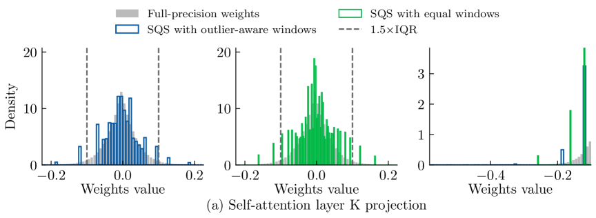
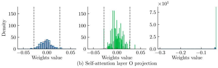
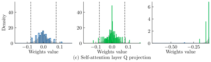
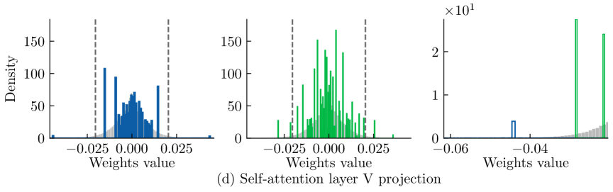
Figure 8: For the compressed weight distributions of the $K$, $O$, $Q$, and $V$ matrices in the self-attention layer of the Llama3.2-1B model, SQS using the outlier-aware window strategy (Left) more effectively preserves the characteristics of the full-precision weight distribution compared to the equal-sized window strategy (Middle). This improvement is particularly noticeable in the left tail region, as highlighted in (Right).

We observe that weight distributions vary significantly across layers, including Gaussian and long-tailed forms. In particular, long-tailed distributions contain a small subset of weights with large magnitudes, as illustrated in Figure 8 for the Llama model. And the previous works (Nagel et al., 2020; Hubara et al., 2021; Frantar and Alistarh, 2022) have demonstrated that layer-wise compression methods lead to better performance.

To address performance degradation arising from such heterogeneous distributions, we extend our proposed method to support layer-wise quantization, where each group of weight parameters within a layer is assigned its own quantization set. This enables each layer to learn and utilize a distinct, trainable quantization set tailored to its distribution.

For layers with long-tailed distributions, we further introduce an outlier-aware windowing strategy. Specifically, the weights $\theta$ in each layer are partitioned into four windows, with two dedicated to capturing the lower and upper tails of the distribution. To identify these tail regions, we apply a standard outlier detection rule based on the $5\times$ interquartile range (IQR): let $q_{1}$ and $q_{3}$ denote the first and third quartiles of the weights, and define $\texttt{IQR}=q_{3}-q_{1}$. The outlier-aware windows are then defined as $[\min(\theta),q_{1}-5\times\texttt{IQR}]$ and $[q_{3}+5\times\texttt{IQR},\max(\theta)]$. Within each of the four windows in every layer, we fit a $K$-component GMM to approximate the local weight distribution.

We adopt the layer-wise quantization scheme with outlier-aware windowing in all our experiments. This approach improves the preservation of extreme values during quantization and enhances robustness across layers. An ablation study evaluating the effectiveness of outlier-aware windowing is presented in Figure 2.

Hyperparameter Configuration.

The number of Gaussian components is set to $K=16$, which balances compression rate and performance degradation. This setting is further analyzed in the case study shown in Figure 3. All models are trained on an NVIDIA H100 GPU with 80GB of memory.

During training and testing, for ResNet-18, ResNet-20, ResNet-32, ResNet-50, ResNet-56, BERT-base, LLaMA3.2-1B, and Qwen2.5-0.5B models, the settings are:

• Training Time: Approximately 30 minutes for ResNet models (ResNet-18 through ResNet-56); 4 hours for BERT-base; 24 hours for both LLaMA3.2-1B and Qwen2.5-0.5B.

• Optimizer: AdamW is used consistently across all models.

• Quantization Learning Rate: $5\times 10^{-4}$ for ResNet-18; $5\times 10^{-5}$ for all other models.

• Pruning Learning Rate: Fixed at $0.012$ for all models.

• Temperature Hyperparameters: $\tau$ in Eq. 6 is set to $5\times 10^{-4}$ and $\tau^{\prime}$ in Eq. 33 is set to $0.0125$.

• Pruning Schedule: A polynomial schedule is used for all models.

Appendix D Experiment Settings

D.1 Experiment settings for benchmark with all baselines

Benchmark compression on ResNet models.

We present experiments using ResNet architectures on the CIFAR-10 and CIFAR-100 datasets. When compressing ResNet models, our method requires fine-tuning over the training dataset, completing the compression process within $10$ epochs. To achieve high compression rates, we represent each layer’s weights with either $4$ or $16$ components (i.e. $K=4$ or $K=16$ for each layer) and apply a sparsity level of $50\%$. As shown in Table 1, our methods compress the models by factors ranging from $16\sim 32\times$ while keeping accuracy drops below $1.3\%$. For example, compressing ResNet-20 by a factor of $16$ results in an accuracy drop of only $0.52\%$. Likewise, compressing ResNet-32 by a factor of $32\times$ yields a minimal accuracy reduction of $1.29\%$. Additionally, we compress ResNet-56 by a factor of $32$, observing an accuracy drop of only $0.84\%$. Compared to other methods, our approach achieves much higher compression rates with smaller decreases in accuracy.

Benchmark compression on Bert-base model.

We further investigate our compression method on attention-based models. We apply our compression model on BERT-base (Devlin et al., 2019) model and test it on the SQuAD V1.1 dataset (Rajpurkar et al., 2016). Similarly, we consider the F1 score drop and compression rate as the evaluation metrics. During the compression process, the BERT model is fine-tuned on the training dataset, with the entire procedure completed within $3$ epochs.

We compressed the BERT model using $K=16$ Gaussian components and pruned $75\%$ of its parameters, leading to a $32\times$ compression rate. We employed layer-wise quantization combined with unstructured pruning to attain these results.

Benchmark compression on Llama and Qwen models.

Due to hardware limitations, we cannot run very large-scale LLMs, which are Llama3.1-8B and Qwen2.5-7B.

D.2 Experiment settings for ablation studies for SQS method

Impact of different window strategies.

For Equal Window strategy, Given a layer of weights $\theta$, we group the weights into 4 windows where each one has an equal window size $\frac{\max(\theta)-\min(\theta)}{4}$. Within each window, a $K$-components GMM is applied to approximate the weights distribution.

Impact of different inference strategies.

The alternative is greedy approach is to greedily select the most likely weight for making predictions on the test set. Specifically, for each quantized weight $\theta_{i}$, we choose the index $k^{*}$ corresponding to the highest posterior probability $\widehat{\phi}_{k^{*}}(\tilde{\theta}_{i})$. The quantized weight is then set to the mean $\mu_{k^{*}}$ of the selected component, and the predicted output $\widehat{y}$ is computed using these selected means. Formally, this greedy inference strategy is given by:

$$\widehat{y}=f(x;\hat{\mu}_{k^{*}}),\qquad k^{*}=\arg\max_{k}\widehat{\phi}_{k}(\tilde{\theta}_{i}),\qquad Q(\theta_{i})=\mu_{k^{*}}.$$ (34)

We empirically compare the greedy inference approach with Bayesian averaging in the ablation study shown in Figure 3.

Impact of different priors.

For comparison, we consider a zero-mean Gaussian distribution as the prior and replace the delta distribution with a Gaussian distribution in the variational family. That is, any $q^{\prime}(\theta)\in\mathcal{F}^{\prime}$ has the form:

$$\tilde{\theta}_{i}|\gamma_{i}\sim\gamma_{i}\sum_{k=1}^{K}\phi_{k}(\theta_{i})\mathcal{N}(\mu_{k},\sigma^{2}_{k})+(1-\gamma_{i})\mathcal{N}(0,\sigma^{2}_{0}), \qquad\gamma_{i}\sim\texttt{Bern}(\tilde{\lambda}_{i}).$$

Based on this, we can get the modified marginal variational distribution $q^{\prime}(\tilde{\theta}_{i})$ as:

$$q^{\prime}(\tilde{\theta}_{i})=\tilde{\lambda}_{i}\sum_{k=1}^{K}\phi_{k}(\theta_{i})\mathcal{N}(\mu_{k},\sigma^{2}_{k})+(1-\tilde{\lambda}_{i})\mathcal{N}(0,\sigma^{2}_{0}).$$ (35)

Thus, following the same reasoning and derivation as we get the equation (8), The Gaussian prior can be obtained by:

$$\Omega^{\prime} =-\mathbb{E}_{q^{\prime}(\tilde{\theta})}\big[\log p(D;\tilde{\theta})\big]+\sum_{i=1}^{T}D_{\mathrm{KL}}\left(q^{\prime}(\tilde{\theta}_{i})\|\mathcal{N}(0,\sigma^{2}_{0})\right)$$

$$=-\mathbb{E}_{q^{\prime}(\tilde{\theta})}\big[\log p(D;\tilde{\theta})\big]+\sum_{i=1}^{T}D_{\mathrm{KL}}\left(q^{\prime}(\tilde{\theta}_{i})\|(\tilde{\lambda}_{i}+(1-\tilde{\lambda}_{i}))\mathcal{N}(0,\sigma^{2}_{0})\right)$$

$$\leq-\mathbb{E}_{q^{\prime}(\tilde{\theta})}\big[\log p(D;\tilde{\theta})\big]+\sum_{i}^{T}\tilde{\lambda}_{i}D_{\mathrm{KL}}\left(\sum_{k=1}^{K}\phi_{k}(\theta_{i})\mathcal{N}(\mu_{k},\sigma^{2}_{k})\Big\|\mathcal{N}(0,\sigma_{0}^{2})\right).$$ (Gaussian prior)

We compare the impact of the above Gaussian prior with the proposed Spike-and-GMM priors and summarize the result in Table 4.

Description of Baselines. For the following lines of baselines, we use the reported results in their papers:

• Optimal Brain Surgeon (OBS) (Hassibi et al., 1993) selects weights for removal from a trained neural network using second-order information.

• BitSplit (Wang et al., 2020a) incrementally constructs quantized values using a squared error metric based on residual errors.

• AdaQuant (Hubara et al., 2021) utilizes STE for direct optimization.

• BRECQ (Li et al., 2021) integrates Fisher information into the optimization process and focuses on the joint optimization of layers within individual residual blocks.

• Exact Optimal Brain Quantization (OBQ) (Frantar and Alistarh, 2022) adapts second-order weight pruning methods to quantization tasks.

• GPTQ (Frantar et al., 2023) employs second-order information for error compensation on calibration sets to speed up generative models.

We adopt their implemented code and use the same setting for training and testing:

• AWQ (Lin et al., 2024) implements activation-aware quantization, selectively bypassing the quantization of key weights. This method is a training-free method, which does not need extra training on the selected dataset.

• DGMS (Dong et al., 2022) is an automated quantization method that utilizes Mixtures of Gaussian to avoid the aforementioned problem. We use their code base and configure it with the same hyperparameters. Their algorithm is trained on the same dataset for fairness of comparison.

Definition of Evaluation Metrics.

Let $K$ denote the number of shared weight vectors. Then, the metric Bits is defined as $\log_{2}K$.

Appendix E Experiment Results for Full-precision Weight Distribution Visualization

We present the visualization of the long-tailed weight distributions for the Llama3.2 model in Figures 6 and 7, and for the Qwen2.5 model in Figures 4 and 5.

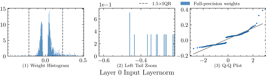
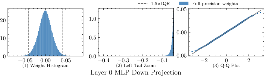
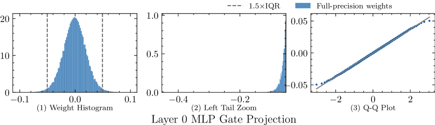
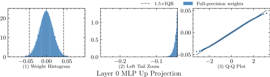
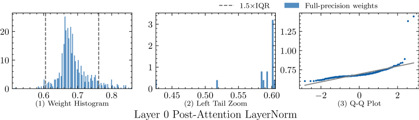
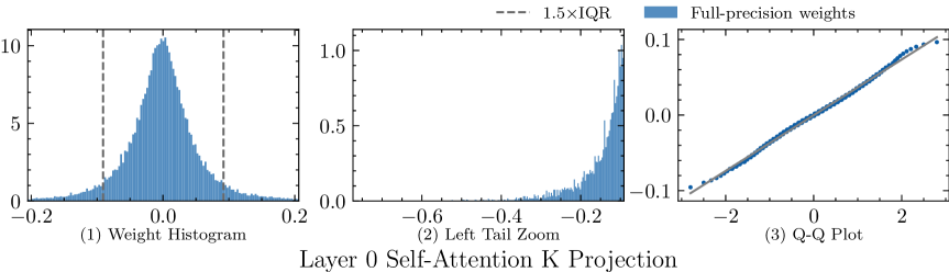
Figure 4: Weight distribution of different layers in Qwen2.5 model (part 1).

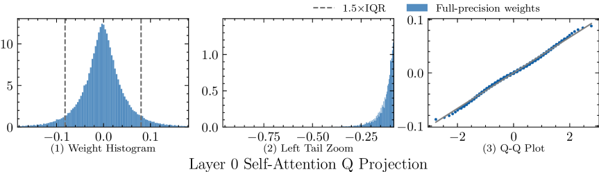
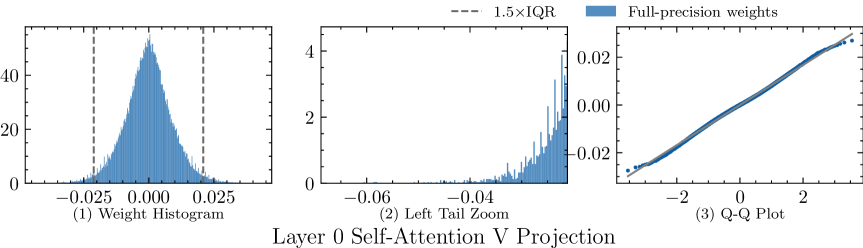
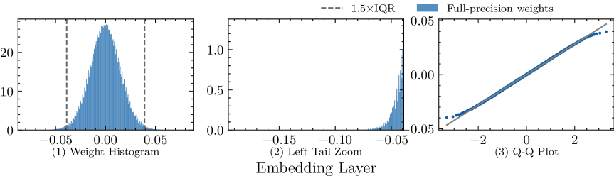
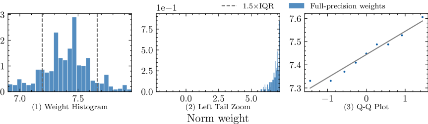
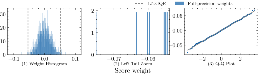
Figure 5: Weight distribution of different layers in Qwen2.5 model (part 2).

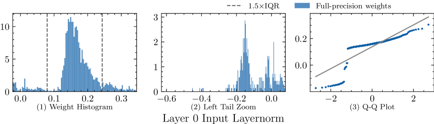
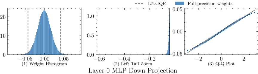
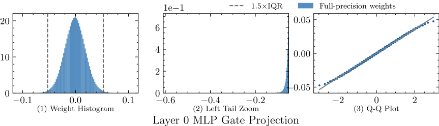
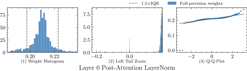
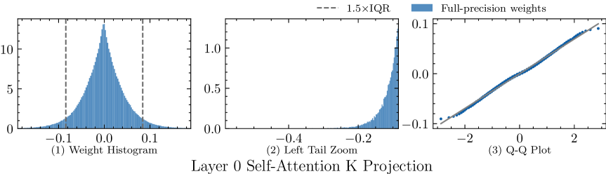
Figure 6: Weight distribution of different layers in Llama3 model (part 1).

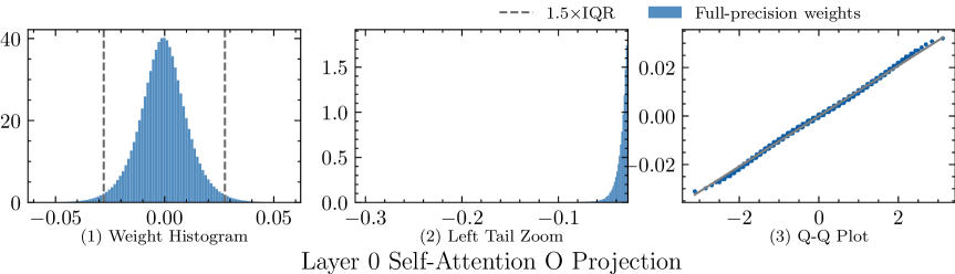
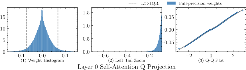
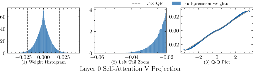
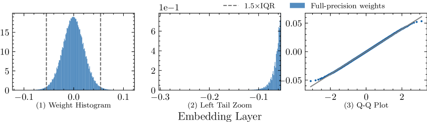
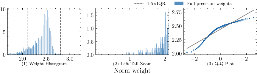
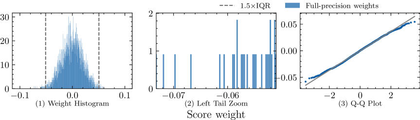
Figure 7: Weight distribution of different layers in Llama3 model (part 2).

References

- Bai et al. (2020) Jincheng Bai, Qifan Song, and Guang Cheng. Efficient variational inference for sparse deep learning with theoretical guarantee. In NeurIPS, volume 33, pages 466–476, 2020.
- Bai et al. (2023) Shipeng Bai, Jun Chen, Xintian Shen, Yixuan Qian, and Yong Liu. Unified data-free compression: Pruning and quantization without fine-tuning. In ICCV, pages 5876–5885, 2023.
- Bai et al. (2022) Yue Bai, Huan Wang, Zhiqiang Tao, Kunpeng Li, and Yun Fu. Dual lottery ticket hypothesis. In ICLR, 2022.
- Banner et al. (2018) Ron Banner, Itay Hubara, Elad Hoffer, and Daniel Soudry. Scalable methods for 8-bit training of neural networks. NeurIPS, 31:5151–5159, 2018.
- Beknazaryan (2022) Aleksandr Beknazaryan. Function approximation by deep neural networks with parameters 0,1 2,1, 2. Journal of Statistical Theory and Practice, 16(1):7, 2022.
- Blei et al. (2017) David M Blei, Alp Kucukelbir, and Jon D McAuliffe. Variational inference: A review for statisticians. Journal of the American statistical Association, 112(518):859–877, 2017.
- Blundell et al. (2015) Charles Blundell, Julien Cornebise, Koray Kavukcuoglu, and Daan Wierstra. Weight uncertainty in neural network. In ICML, pages 1613–1622, 2015.
- Boucheron et al. (2013) Stephane Boucheron, Gabor Lugosi, and Pascal Massart. Concentration inequalities: A nonasymptotic theory of independence. Oxford University press, 2013.
- Buciluǎ et al. (2006) Cristian Buciluǎ, Rich Caruana, and Alexandru Niculescu-Mizil. Model compression. In ICDM, pages 535–541, 2006.
- Chérief-Abdellatif (2020) Badr-Eddine Chérief-Abdellatif. Convergence rates of variational inference in sparse deep learning. In ICML, pages 1831–1842, 2020.
- Chérief-Abdellatif and Alquier (2018) Badr-Eddine Chérief-Abdellatif and Pierre Alquier. Consistency of variational bayes inference for estimation and model selection in mixtures. Electronic Journal of Statistics, 12(2):2995 – 3035, 2018.
- Choudhary et al. (2020) Tejalal Choudhary, Vipul Mishra, Anurag Goswami, and Jagannathan Sarangapani. A comprehensive survey on model compression and acceleration. Artificial Intelligence Review, 53:5113–5155, 2020.
- Courbariaux and Bengio (2016) Matthieu Courbariaux and Yoshua Bengio. Binarynet: Training deep neural networks with weights and activations constrained to +1 or -1. CoRR, abs/1602.02830, 2016.
- Courbariaux et al. (2015) Matthieu Courbariaux, Yoshua Bengio, and Jean-Pierre David. Binaryconnect: Training deep neural networks with binary weights during propagations. NeurIPS, 28:3123–3131, 2015.
- Csiszár (1975) Imre Csiszár. I-divergence geometry of probability distributions and minimization problems. The annals of probability, pages 146–158, 1975.
- De Sa et al. (2018) Christopher De Sa, Megan Leszczynski, Jian Zhang, Alana Marzoev, Christopher R Aberger, Kunle Olukotun, and Christopher Ré. High-accuracy low-precision training. arXiv preprint arXiv:1803.03383, 2018.
- Dekking (2005) Frederik Michel Dekking. A Modern Introduction to Probability and Statistics: Understanding why and how. Springer Science & Business Media, 2005.
- Deng et al. (2019) Wei Deng, Xiao Zhang, Faming Liang, and Guang Lin. An adaptive empirical bayesian method for sparse deep learning. In NeurIPS, volume 32, pages 5564–5574, 2019.
- Dettmers et al. (2023) Tim Dettmers, Artidoro Pagnoni, Ari Holtzman, and Luke Zettlemoyer. Qlora: Efficient finetuning of quantized llms. In NeurIPS, 2023.
- Devlin et al. (2019) Jacob Devlin, Ming-Wei Chang, Kenton Lee, and Kristina Toutanova. BERT: pre-training of deep bidirectional transformers for language understanding. In NAACL, pages 4171–4186, 2019.
- Dong et al. (2022) Runpei Dong, Zhanhong Tan, Mengdi Wu, Linfeng Zhang, and Kaisheng Ma. Finding the task-optimal low-bit sub-distribution in deep neural networks. In ICML, pages 5343–5359. PMLR, 2022.
- Dong et al. (2017) Xin Dong, Shangyu Chen, and Sinno Pan. Learning to prune deep neural networks via layer-wise optimal brain surgeon. NeurIPS, 30:4857–4867, 2017.
- Frankle and Carbin (2019) Jonathan Frankle and Michael Carbin. The lottery ticket hypothesis: Finding sparse, trainable neural networks. In ICLR, 2019.
- Frantar and Alistarh (2022) Elias Frantar and Dan Alistarh. Optimal brain compression: A framework for accurate post-training quantization and pruning. NeurIPS, 35:4475–4488, 2022.
- Frantar et al. (2023) Elias Frantar, Saleh Ashkboos, Torsten Hoefler, and Dan Alistarh. OPTQ: Accurate quantization for generative pre-trained transformers. In The Eleventh ICLR, 2023.
- Gholami et al. (2022) Amir Gholami, Sehoon Kim, Zhen Dong, Zhewei Yao, Michael W Mahoney, and Kurt Keutzer. A survey of quantization methods for efficient neural network inference. In Low-power computer vision, pages 291–326. Chapman and Hall/CRC, 2022.
- Gou et al. (2021) Jianping Gou, Baosheng Yu, Stephen J Maybank, and Dacheng Tao. Knowledge distillation: A survey. International Journal of Computer Vision, 129(6):1789–1819, 2021.
- Guo et al. (2016) Yiwen Guo, Anbang Yao, and Yurong Chen. Dynamic network surgery for efficient dnns. NeurIPS, 29:1379–1387, 2016.
- Gupta et al. (2015) Suyog Gupta, Ankur Agrawal, Kailash Gopalakrishnan, and Pritish Narayanan. Deep learning with limited numerical precision. In ICML, pages 1737–1746, 2015.
- Han et al. (2016) Song Han, Huizi Mao, and William J. Dally. Deep compression: Compressing deep neural network with pruning, trained quantization and huffman coding. In ICLR, 2016.
- Hassibi et al. (1993) Babak Hassibi, David G Stork, and Gregory J Wolff. Optimal brain surgeon and general network pruning. In IEEE international conference on neural networks, pages 293–299. IEEE, 1993.
- Hershey and Olsen (2007) John R. Hershey and Peder A. Olsen. Approximating the kullback leibler divergence between gaussian mixture models. In IEEE International Conference on Acoustics, Speech, and Signal Processing, pages 317–320. IEEE, 2007.
- Hubara et al. (2018) Itay Hubara, Matthieu Courbariaux, Daniel Soudry, Ran El-Yaniv, and Yoshua Bengio. Quantized neural networks: Training neural networks with low precision weights and activations. Journal of Machine Learning Research, 18(187):1–30, 2018.
- Hubara et al. (2021) Itay Hubara, Yury Nahshan, Yair Hanani, Ron Banner, and Daniel Soudry. Accurate post training quantization with small calibration sets. In ICML, pages 4466–4475, 2021.
- Ishwaran and Rao (2005) Hemant Ishwaran and J Sunil Rao. Spike and slab variable selection: frequentist and bayesian strategies. Annals of Statistics, 33:730–73, 2005.
- Jacob et al. (2018) Benoit Jacob, Skirmantas Kligys, Bo Chen, Menglong Zhu, Matthew Tang, Andrew Howard, Hartwig Adam, and Dmitry Kalenichenko. Quantization and training of neural networks for efficient integer-arithmetic-only inference. In CVPR, pages 2704–2713, 2018.
- Jordan et al. (1999) Michael I Jordan, Zoubin Ghahramani, Tommi S Jaakkola, and Lawrence K Saul. An introduction to variational methods for graphical models. Machine learning, 37:183–233, 1999.
- Kumar et al. (2025) Tanishq Kumar, Zachary Ankner, Benjamin Frederick Spector, Blake Bordelon, Niklas Muennighoff, Mansheej Paul, Cengiz Pehlevan, Christopher Re, and Aditi Raghunathan. Scaling laws for precision. In ICLR, 2025.
- LeCun et al. (1989) Yann LeCun, John Denker, and Sara Solla. Optimal brain damage. NeurIPS, 2:598–605, 1989.
- Li et al. (2017) Hao Li, Asim Kadav, Igor Durdanovic, Hanan Samet, and Hans Peter Graf. Pruning filters for efficient convnets. In ICLR, 2017.
- Li et al. (2021) Yuhang Li, Ruihao Gong, Xu Tan, Yang Yang, Peng Hu, Qi Zhang, Fengwei Yu, Wei Wang, and Shi Gu. {BRECQ}: Pushing the limit of post-training quantization by block reconstruction. In ICLR, 2021.
- Lin et al. (2024) Ji Lin, Jiaming Tang, Haotian Tang, Shang Yang, Wei-Ming Chen, Wei-Chen Wang, Guangxuan Xiao, Xingyu Dang, Chuang Gan, and Song Han. AWQ: activation-aware weight quantization for on-device LLM compression and acceleration. In Annual Conference on Machine Learning and Systems, 2024.
- Lin et al. (2025) Moule Lin, Shuhao Guan, Weipeng Jing, Goetz Botterweck, and Andrea Patane. Stochastic weight sharing for bayesian neural networks. In AISTATS, volume 258 of Proceedings of Machine Learning Research, pages 4519–4527. PMLR, 2025.
- Liu et al. (2018) Chenxi Liu, Barret Zoph, Maxim Neumann, Jonathon Shlens, Wei Hua, Li-Jia Li, Li Fei-Fei, Alan Yuille, Jonathan Huang, and Kevin Murphy. Progressive neural architecture search. In ECCV, pages 19–34, 2018.
- Liu et al. (2025) Kai Liu, Qian Zheng, Kaiwen Tao, Zhiteng Li, Haotong Qin, Wenbo Li, Yong Guo, Xianglong Liu, Linghe Kong, Guihai Chen, Yulun Zhang, and Xiaokang Yang. Low-bit model quantization for deep neural networks: A survey, 2025. URL https://arxiv.org/abs/2505.05530.
- Louizos et al. (2017) Christos Louizos, Karen Ullrich, and Max Welling. Bayesian compression for deep learning. In NeurIPS, volume 30, pages 3288–3298, 2017.
- Louizos et al. (2018) Christos Louizos, Max Welling, and Diederik P. Kingma. Learning sparse neural networks through regularization. In ICLR, 2018.
- Louizos et al. (2019) Christos Louizos, Matthias Reisser, Tijmen Blankevoort, Efstratios Gavves, and Max Welling. Relaxed quantization for discretized neural networks. In ICLR, 2019.
- Marchesi et al. (1993) Michele Marchesi, Gianni Orlandi, Francesco Piazza, and Aurelio Uncini. Fast neural networks without multipliers. IEEE transactions on Neural Networks, 4(1):53–62, 1993.
- Nagel et al. (2020) Markus Nagel, Rana Ali Amjad, Mart Van Baalen, Christos Louizos, and Tijmen Blankevoort. Up or down? adaptive rounding for post-training quantization. In ICML, pages 7197–7206, 2020.
- Nielsen et al. (2025) Jacob Nielsen, Peter Schneider-Kamp, and Lukas Galke. Continual quantization-aware pre-training: When to transition from 16-bit to 1.58-bit pre-training for bitnet language models? In ACL (Findings), pages 13483–13493. Association for Computational Linguistics, 2025.
- Park et al. (2019) Wonpyo Park, Dongju Kim, Yan Lu, and Minsu Cho. Relational knowledge distillation. In CVPR, pages 3967–3976, 2019.
- Radford et al. (2018) Alec Radford, Karthik Narasimhan, Tim Salimans, and Ilya Sutskever. Improving language understanding by generative pre-training. 2018.
- Rajpurkar et al. (2016) Pranav Rajpurkar, Jian Zhang, Konstantin Lopyrev, and Percy Liang. Squad: 100, 000+ questions for machine comprehension of text. In EMNLP, pages 2383–2392, 2016.
- Rastegari et al. (2016) Mohammad Rastegari, Vicente Ordonez, Joseph Redmon, and Ali Farhadi. Xnor-net: Imagenet classification using binary convolutional neural networks. In ECCV, pages 525–542. Springer, 2016.
- Roth and Pernkopf (2018) Wolfgang Roth and Franz Pernkopf. Bayesian neural networks with weight sharing using dirichlet processes. IEEE transactions on pattern analysis and machine intelligence, 42(1):246–252, 2018.
- Shayer et al. (2018) Oran Shayer, Dan Levi, and Ethan Fetaya. Learning discrete weights using the local reparameterization trick. In ICLR, 2018. URL https://openreview.net/forum?id=BySRH6CpW.
- Singh and Alistarh (2020) Sidak Pal Singh and Dan Alistarh. Woodfisher: Efficient second-order approximation for neural network compression. In NeurIPS, volume 33, pages 18098–18109, 2020.
- Sun et al. (2019) Xiao Sun, Jungwook Choi, Chia-Yu Chen, Naigang Wang, Swagath Venkataramani, Vijayalakshmi Viji Srinivasan, Xiaodong Cui, Wei Zhang, and Kailash Gopalakrishnan. Hybrid 8-bit floating point (hfp8) training and inference for deep neural networks. NeurIPS, 32:4901–4910, 2019.
- Sun et al. (2022) Yan Sun, Qifan Song, and Faming Liang. Consistent sparse deep learning: Theory and computation. Journal of the American Statistical Association, 117(540):1981–1995, 2022.
- Sze et al. (2017) Vivienne Sze, Yu-Hsin Chen, Tien-Ju Yang, and Joel S Emer. Efficient processing of deep neural networks: A tutorial and survey. Proceedings of the IEEE, 105(12):2295–2329, 2017.
- Touvron et al. (2023) Hugo Touvron, Thibaut Lavril, Gautier Izacard, Xavier Martinet, Marie-Anne Lachaux, Timothée Lacroix, Baptiste Rozière, Naman Goyal, Eric Hambro, Faisal Azhar, et al. Llama: Open and efficient foundation language models. arXiv preprint arXiv:2302.13971, 2023.
- Ullrich et al. (2017) Karen Ullrich, Edward Meeds, and Max Welling. Soft weight-sharing for neural network compression. In ICLR, 2017.
- Wang et al. (2019) Chaoqi Wang, Roger Grosse, Sanja Fidler, and Guodong Zhang. Eigendamage: Structured pruning in the kronecker-factored eigenbasis. In ICML, pages 6566–6575, 2019.
- Wang et al. (2020a) Peisong Wang, Qiang Chen, Xiangyu He, and Jian Cheng. Towards accurate post-training network quantization via bit-split and stitching. In ICML, pages 9847–9856, 2020a.
- Wang et al. (2025) Ruizhe Wang, Yeyun Gong, Xiao Liu, Guoshuai Zhao, Ziyue Yang, Baining Guo, Zheng-Jun Zha, and Peng CHENG. Optimizing large language model training using FP4 quantization. In ICLR, 2025.
- Wang et al. (2020b) Tianzhe Wang, Kuan Wang, Han Cai, Ji Lin, Zhijian Liu, Hanrui Wang, Yujun Lin, and Song Han. Apq: Joint search for network architecture, pruning and quantization policy. In CVPR, pages 2078–2087, 2020b.
- Wang et al. (2020c) Ying Wang, Yadong Lu, and Tijmen Blankevoort. Differentiable joint pruning and quantization for hardware efficiency. In ECCV, pages 259–277, 2020c.
- Wei et al. (2022) Xiuying Wei, Yunchen Zhang, Xiangguo Zhang, Ruihao Gong, Shanghang Zhang, Qi Zhang, Fengwei Yu, and Xianglong Liu. Outlier suppression: Pushing the limit of low-bit transformer language models. In NeurIPS, 2022.
- Wortsman et al. (2023) Mitchell Wortsman, Tim Dettmers, Luke Zettlemoyer, Ari Morcos, Ali Farhadi, and Ludwig Schmidt. Stable and low-precision training for large-scale vision-language models. NeurIPS, 36:10271–10298, 2023.
- Wu et al. (2018) Shuang Wu, Guoqi Li, Feng Chen, and Luping Shi. Training and inference with integers in deep neural networks. arXiv preprint arXiv:1802.04680, 2018.
- Xia et al. (2024) Mengzhou Xia, Tianyu Gao, Zhiyuan Zeng, and Danqi Chen. Sheared LLaMA: Accelerating language model pre-training via structured pruning. In ICLR, 2024.
- Xu et al. (2020) Canwen Xu, Wangchunshu Zhou, Tao Ge, Furu Wei, and Ming Zhou. Bert-of-theseus: Compressing BERT by progressive module replacing. In EMNLP, pages 7859–7869, 2020.
- Yin et al. (2019) Penghang Yin, Jiancheng Lyu, Shuai Zhang, Stanley J. Osher, Yingyong Qi, and Jack Xin. Understanding straight-through estimator in training activation quantized neural nets. In ICLR, 2019.
- You et al. (2019) Zhonghui You, Kun Yan, Jinmian Ye, Meng Ma, and Ping Wang. Gate decorator: Global filter pruning method for accelerating deep convolutional neural networks. NeurIPS, 32:2130–2141, 2019.
- Zhang et al. (2018) Dongqing Zhang, Jiaolong Yang, Dongqiangzi Ye, and Gang Hua. Lq-nets: Learned quantization for highly accurate and compact deep neural networks. In ECCV, pages 365–382, 2018.
- Zhang et al. (2022) Qingru Zhang, Simiao Zuo, Chen Liang, Alexander Bukharin, Pengcheng He, Weizhu Chen, and Tuo Zhao. Platon: Pruning large transformer models with upper confidence bound of weight importance. In ICML, pages 26809–26823, 2022.
- Zhu et al. (2017) Chenzhuo Zhu, Song Han, Huizi Mao, and William J. Dally. Trained ternary quantization. In ICLR, 2017.
- Zhu and Gupta (2017) Michael Zhu and Suyog Gupta. To prune, or not to prune: exploring the efficacy of pruning for model compression. arXiv preprint arXiv:1710.01878, 2017.