Beyond the Carnot limit: work extraction via an entropy battery

Abstract

We explore the consequences of generalized thermodynamics, as interpreted from the perspective of information theory, on an ensemble’s capacity to extract energetic work. We demonstrate that by utilizing unitary heat engines of different kinds, we can capitalize on the full entropy capacity of the ensemble across multiple conserved quantities. This leads to the extraction of energetic work with efficiencies surpassing the standard Carnot efficiency limit, all the while running at maximum power. This is achieved without requiring modified thermal sources, which is a method commonly used in the field of quantum heat engines. We pay particular attention to spin angular momentum, and show that when treated as a mutually independent conserved quantity, spin baths exhibit thermodynamic behaviour analogous to conventional heat baths, with corresponding quantities and models. This includes spin-analogous heat capacities, Einstein solid and Debye models, entropic responses, and Bose-Einstein and Fermi-Dirac statistics. Spin baths also follow the fluctuation-dissipation theorem. Further, we examine the role of particle statistics in determining the maximum entropy capacity of the battery. In doing so, we argue that indistinguishability is necessary for interactions to occur, motivating a perspective in which information itself is treated as the indistinguishable property of particles, with information (in the form of coherence) transferable between both physical degrees of freedom such as energy and spin, and particles when the system acts unitarily. This work will find application in fields that require near energy degenerate spin statistics, such as in spinor Bose–Einstein condensates and spintronics. Further, our method will have implications for the fields of quantum heat engines, quantum batteries, quantum error correction, and information and resource theories.

I Introduction

Born out of the Industrial Revolution, heat engines provided not only practical utility but, more importantly, a theoretical framework for describing some of the most fundamental principles of nature. The pursuit of increasingly powerful and efficient engines, refrigerators, and related devices, driven by both technological ambition and the intellectual curiosity of figures such as Carnot and Clausius [1], led to the formulation of the four laws of thermodynamics, which govern the dynamics of heat and energy. The need to explain the emergence of these laws from the microscopic constituents of thermodynamic systems lead to statistical mechanics, a theory that successfully described the macroscopic properties of the ensemble using probability and statistical techniques. Maxwell, by utilizing statistical mechanics, proposed a mechanism by which an entity with sufficient knowledge of the microscopic states could violate the laws of thermodynamics [2], in what came to be known as Maxwell’s demon.

Szilard [3], Landauer [4], and Bennett [5] each contributed, at times indirectly, to the resolution of this paradox, with Bennett ultimately recognising that such a demon would only operate for as long as it’s memory has capacity to store information about the state of the system. If this capacity were saturated, as would occur for a demon constrained by finite physical resources, no further work could be extracted from the system. Bennett showed, using Landauer’s principal, that the energetic cost of erasing the demon’s memory would be greater-than or equal-to the amount of work extracted during the engine cycles, therefore closing the paradox.

The roles of Information and entropy (the latter being the lack of the former) in thermodynamics became a recurring theme in the study of thermodynamic systems, even prior to the resolution of the demon paradox. Jaynes, from the perspective of information theory, generalized statistical mechanics to include arbitrary conserved quantities, therefore removing the special treatment given to energy [6, 7]. His rational can be intuitively understood by recognising that the time invariant nature of conserved quantities must allow for the storage of information. Vaccaro and Barnett later used Jaynes’s principle to show how the erasure of information in the Maxwell demon thought experiment can be performed using spin angular momentum [8, 9], leading to the development of memory powered heat engines [10] and gas spin heat engines [11]. The application of Jayne’s work to quantum systems has also led to developments in generalized heat baths, quantum batteries, and resource theories [12, 13, 14]. With a renewed focus on information as a general resource, it appears as though thermodynamics is not describing the flow of energy and heat, but instead the flow of information and entropy at the most fundamental level, with conserved quantities acting merely as the physical degrees of freedom for which the information is encoded. Yet, the concept of generalized information as a resource has not been widely utilized by the scientific community, as no clear practicality has emerged for applying thermodynamics in this manner. This paper provides one such practicality.

To be precise, the term “information” is coherence, corresponding to certainty in the system’s state. For instance, a pure state conveys unambiguous information about a particle’s position in state space and thus the coherence of the state is a manifestation of information. For an ensemble of interacting particles, information is extended to include coherent correlations, or entanglement. Entropy on the other hand is a measure of the “mixed”, or classical uncertainty of the conserved quantity, with entropy representing the lack of information about the particle’s state. Whether this entropy is an ‘anthropomorphic’ by-product of our ignorance as an observer [15], or is as physical as the conserved quantities themselves, the act of obtaining information and thus reducing the systems entropy takes physical resources [5, 8], thus entropy must be treated as a resource itself.

The promises of modern resource theories, quantum batteries, and quantum heat engines include: collective power enhancement in the charging of quantum batteries [16], heat engines utilizing non-energetic cold baths [10, 11], the saturation and surpassing of the classical Carnot energy efficiency limit [17, 18], and methods of error correction in quantum computers [19, 20]. Information and resource theories have also found broad application across the fields of quantum state amplification and metrology [21, 22, 23]. Of the works presented thus far, none have explicitly explored how the entropy capacity of an ensemble changes once other conserved quantities are introduced. More importantly, none have explored how coherent coupling mechanisms between conserved quantities, such as those used by [10, 11], change both the efficiency of energetic work extraction and the total work extractable. [24, 25, 12] have independently explored the reversible exchange of conserved quantities within the framework of generalized thermodynamics; however, they did not address the extent to which these methods influence the practicality of applying such principles to large ensembles for performing useful work.

Furthermore, a common approach used in the field of quantum heat engines to surpass the Carnot efficiency limit is to exploit intrinsic quantum coherence in the thermal bath, for example via squeezed-thermal sources [26, 27, 28], or through induced quantum coherence [29, 30, 31]. However, introducing coherence into a thermal system incurs an energy cost under the second law of thermodynamics, as such non-thermal states are ‘purer’ than the corresponding thermal state at the same temperature, which by definition maximizes entropy. Taking the totality of the resources required to run such quantum heat engines above the Carnot limit, one finds no such energy efficiency gain was made. This is reflected in the fact that such devices operate below the generalized Carnot limit [32], which accounts for the efficiency gains achievable with engineered non-thermal states. Furthermore, the field of quantum heat engines is often limited in total extractable work as it generally relies on individual quantum systems, such as single ions or molecules, where quantum effects significantly influence the engine cycle. In general, the Carnot efficiency limit for two thermal sources has prevailed as unsurpassable, with quantum systems only possibly saturating the limit [17].

We argue, in the spirit of Jaynes, Vaccaro and others, that a reinterpretation of thermodynamics into a purely informational basis allows for an intuitive interpretation of the operation of all adiabatic and unitary heat engines, with them now acting as mechanisms that transfer coherent information and incoherent entropy across every conserved quantity. This interpretation applies also to the engines we use in what we call the entropy battery. The entropy battery, and this paper, will also consider conserved quantities that meet the criteria of being experimentally accessible and controllable.

There are 8 conserved quantities for which one can in principle encode information. This is because there exist eight fundamental physical symmetries, each associated with a corresponding conservation law and conserved quantity, in accordance with Noether’s theorem [33, 34]. The known conserved quantities are presented in Table 1.

Conserved quantity	‘Heat’ analogue	‘Work’ analogue
Energy	heat $Q$	work $W$
Spin angular momentum	spin therm $\mathcal{Q}$	spin labor $\mathcal{L}$
Linear momentum	Generalized heat $\mathbb{Q}$	Generalized work $\mathbb{W}$
Lorentz 3-vector boost
Electric charge
Color charge
Weak isospin

Table 1: The known conserved quantities as derived from continuous physical symmetries according to Noether’s theorem, excluding Baryon, Lepton difference. Also shown are the known analogous definitions of ‘heat’ and ‘work’ for these conserved quantities, with $\mathbb{Q}$ and $\mathbb{W}$ in place for the quantities without literature definitions. Energy, linear momentum, and the Lorentz 3-vector boost may be defined on both discrete and continuous state spaces, spin angular momentum, electric charge, color charge, and weak isospin are intrinsically discrete and bounded. The generalized heat and work are assumed to exist for these conserved quantities based on the commentary in this paper, although the application of these quantities as useful thermodynamic properties is questionable with the current state of technology.

Among the eight conserved quantities, only energy and spin angular momentum satisfy the criteria of accessibility and controllability, with systems such as Bose–Einstein condensates and trapped atoms allowing controllable preparation of both thermal motion and internal spin states. We will therefore focus our efforts in this paper on energy in a single degree of freedom and the z-component of spin angular momentum, without loss of generality.

We anticipate that the entropy battery will have applications extending beyond future high-efficiency heat engines and batteries. For example, heat storage in environments where waste heat removal is challenging (e.g., the vacuum of space), mitigation of entropy-induced noise in quantum measurements such as those in quantum computing, and refrigeration with efficiencies surpassing those of present technologies. Separately, our analysis of information thermodynamics applied to spin angular momentum will have application in fields that require a description of ensemble spin state statistics in energy degenerate regimes, such as spinor BEC’s and spintronics.

The results of the entropy battery and the corresponding spin thermodynamics are presented in §II, followed by a discussion of entropy capacity maximization in §III. Model derivations are provided in the Appendix.

II The entropy battery

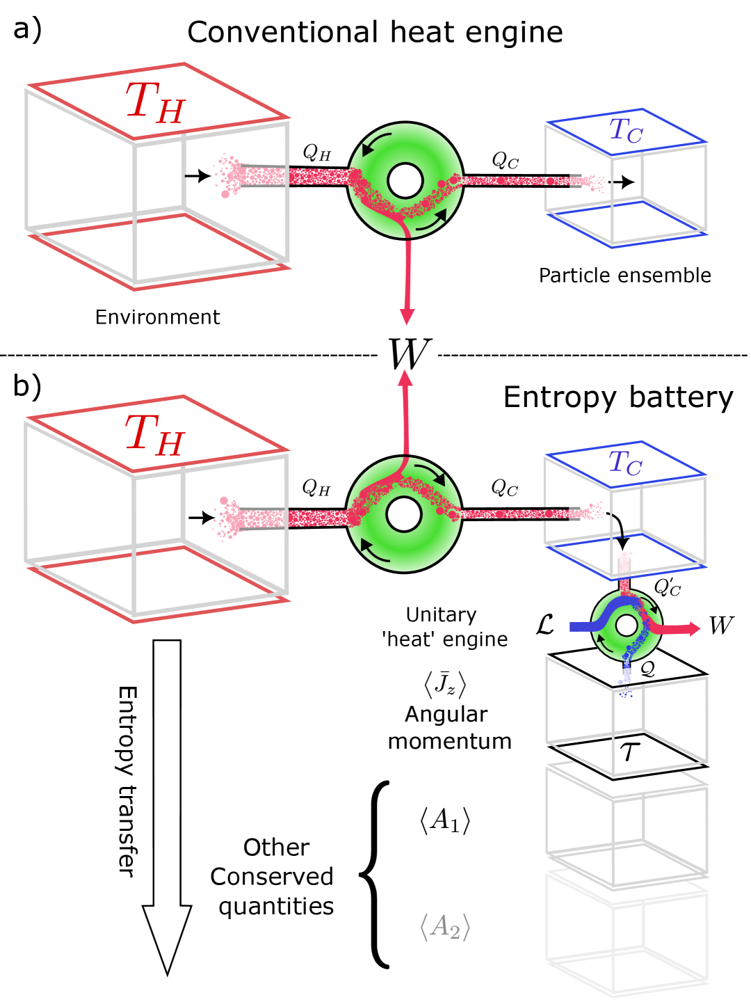
Figure 1: Overview of (a) a conventional Carnot heat engine between hot and cold baths, and (b) the entropy battery. In (b), the equivalent conserved quantity ‘heat’ baths with general conserved quantity $\braket{A_{m}}$ are represented by black cubes aligned vertically. Energy couples to spin angular momentum within the entropy battery via a unitary “heat engine,” realized experimentally through coherent Raman transitions [10, 11]. Spin labor $\mathcal{L}$ supplied by the entropy battery enables the conversion of heat energy into work. There aren’t any equivalent coupling mechanisms for the other conserved quantities. Entropy from the environmental heat bath is transferred into the battery’s internal baths (energy, spin, etc.), enhancing work extraction until their entropy capacities are saturated or equilibrium is reached. As these other conserved quantity ‘heat’ baths reside within the battery’s particles, the scheme achieves a higher volumetric work density than conventional heat engines.

In Fig.1 we present an overview of the entropy transfer process during the operation of the entropy battery. In our model, we assume the energy and z-component of spin angular momentum conserved quantities are mutually independent, making the entropy of the ensemble initially extensive over energy $\mathbb{S}_{\text{energy}}$ and spin $\mathbb{S}_{\text{spin}}$,

$$\mathbb{S}_{\text{battery}}=\mathbb{S}_{\text{energy}}+\mathbb{S}_{\text{spin}}.$$ (1)

Since spin angular momentum is independent of any other quantity in our model, it behaves as an independent thermodynamic system. Table 2 summarizes the analogous spin-angular-momentum thermodynamic relations derived in this paper, with derivations provided in Appendices A–E, including the four laws of generalized thermodynamics.

	Thermodynamic property	Energy	Spin angular momentum
	Entropy	$\displaystyle\mathbb{S}_{E}=\ln(Z_{E})+\beta\braket{E}$	$\displaystyle\mathbb{S}_{s}=\ln(Z_{s})+\gamma\braket{\bar{J}_{z}}$	(2)
	Partition function ($\Omega=\text{microstates}$)	$\displaystyle Z_{E}=\sum_{\Omega}e^{-\beta E(\Omega)}$	$\displaystyle Z_{s}=\sum_{\Omega}e^{-\gamma J(\Omega)}$	(3)
	Inverse temperature	$\displaystyle\beta=\frac{1}{k_{B}T}$	$\displaystyle\gamma=\frac{1}{\tau}$	(4)
	Entropy-energy/ spin relation	$\displaystyle\frac{\partial\mathbb{S}_{E}}{\partial\braket{E}}=\frac{1}{T}$	$\displaystyle\frac{\partial\mathbb{S}_{s}}{\partial\braket{\bar{J}_{z}}}=\frac{1}{\tau}$	(5)
	Average conserved quantity	$\displaystyle\braket{E}=-\frac{\partial}{\partial\beta}\ln(Z_{E})=T^{2}\frac{\partial}{\partial T}\ln(Z_{E})$	$\displaystyle\braket{\bar{J}_{z}}=-\frac{\partial}{\partial\gamma}\ln(Z_{s})=\tau^{2}\frac{\partial}{\partial\tau}\ln(Z_{s})$	(6)
	Heat capacity/ waste response	$\displaystyle C_{V}=\left(\frac{\partial\braket{E}}{\partial T}\right)_{V}$	$\displaystyle C_{s}=\frac{d\braket{\bar{J}_{z}}}{d\tau}$	(7)
	Entropic response	$\displaystyle\frac{1}{T}C_{V}=\left(\frac{\partial\mathbb{S}_{E}}{\partial T}\right)_{V}$	$\displaystyle\frac{1}{\tau}C_{s}=\frac{d\mathbb{S}_{s}}{d\tau}$	(8)
	Heat/spin therm	$\displaystyle Q=\int C_{V}dT$	$\displaystyle\mathcal{Q}=\int C_{s}d\tau$	(9)
	Bosonic heat for solids in the thermodynamic limit	$\displaystyle\frac{Q}{N}=\frac{1}{2}\sum_{j}\varepsilon_{j}(\coth(\varepsilon_{j}/2k_{B}T)-1)$	$\displaystyle\frac{\mathcal{Q}}{N}=\frac{1}{2}\sum_{j=1}^{2S}j\left(\coth(j/2\tau)-1\right)$	(10)
	Work/spin labor [9]	$\displaystyle W=Q_{1}+Q_{2}$	$\displaystyle\mathcal{L}=\mathcal{Q}_{1}+\mathcal{Q}_{2}$	(11)
Four lawshi	Zero’th law	$\displaystyle\lim_{T\rightarrow 0}\mathbb{S}_{E}=0$	$\displaystyle\lim_{\tau\rightarrow 0}\mathbb{S}_{s}=0$	(12)
	First law (closed system)	$\displaystyle\delta\braket{E}=0$	$\displaystyle\delta\braket{\bar{J}_{z}}=0$	(13)
	Second law (closed system)	$\displaystyle\delta\mathbb{S}_{E}=0$	$\displaystyle\delta\mathbb{S}_{s}=0$	(14)
	Third law	$\displaystyle T_{1}=T_{2}$	$\displaystyle\tau_{1}=\tau_{2}$	(15)
Ensemble statisticshihihihihihihihi	Bose-Einstein/Fermi-dirac ($\mp$) distributions [35]	$\displaystyle\braket{n_{\varepsilon}}=\frac{1}{e^{(\varepsilon-\mu)/k_{B}T}\mp 1}$	$\displaystyle\braket{n_{j}}=\frac{1}{e^{(j-S)/\tau}\mp 1}$	(16)
	Distinguishable heat capacity/waste response [36]	$\displaystyle\frac{C_{V}}{N}=\frac{1}{k_{B}T^{2}}\times\text{Var}(E(T))$	$\displaystyle\frac{C_{s}}{N}=\frac{1}{\tau^{2}}\times\text{Var}(\bar{J}_{z}(\tau))$	(17)
	Einstein Solid model per degree of freedom [37]	$\displaystyle\frac{C_{V}}{N}=\frac{1}{4k_{B}T^{2}}\,\times\,\frac{\varepsilon}{\sinh^{2}(\varepsilon/2k_{B}T)}$	$\displaystyle\frac{C_{s}}{N}=\frac{1}{4\tau^{2}}\,\times\,\frac{1}{\sinh^{2}(1/2\tau)}$	(18)
	Bosonic heat capacity/ waste response	$\displaystyle\frac{C_{V}}{N}=\frac{1}{4k_{B}T^{2}}\sum_{j}\frac{\varepsilon_{j}^{2}}{\sinh^{2}(\varepsilon_{j}/2k_{B}T)}$	$\displaystyle\frac{C_{s}}{N}=\frac{1}{4\tau^{2}}\sum_{j=1}^{2S}\frac{j^{2}}{\sinh^{2}(j/2\tau)}$	(19)
	Debye model per degree of freedom [37]	$\displaystyle\frac{C_{V}}{N}=\frac{3}{4k_{B}T^{2}\varepsilon_{D}^{2}}\int_{0}^{\varepsilon_{D}}\frac{\varepsilon_{j}^{2}}{\sinh^{2}(\varepsilon_{j}/2k_{B}T)}\varepsilon_{j}^{2}d\varepsilon$	$\displaystyle\frac{C_{s}}{N}=\frac{3}{4\tau^{2}(2S)^{2}}\int_{0}^{2S}\frac{j^{2}}{\sinh^{2}(j/2\tau)}j^{2}dj$	(20)
	Distinguishable Entropy capacity	$\mathbb{S}_{\text{max}}=N\ln(d_{E})$	$\displaystyle\mathbb{S}_{\text{max}}=N\ln(d_{s})$	(21)
	Bosonic Entropy capacity	$\mathbb{S}_{\text{max}}=\ln\begin{pmatrix}N+d_{E}-1\\ d_{E}-1\end{pmatrix}$	$\displaystyle\mathbb{S}_{\text{max}}=\ln\begin{pmatrix}N+d_{s}-1\\ d_{s}-1\end{pmatrix}$	(22)
	Fermionic Entropy capacity	$\mathbb{S}_{\text{max}}=\ln\begin{pmatrix}d_{E}\\ N\end{pmatrix}$	$\displaystyle\mathbb{S}_{\text{max}}=\ln\begin{pmatrix}d_{s}\\ N\end{pmatrix}$	(23)

Table 2: Summary of the spin-analogous thermodynamic properties. In these expressions, $\braket{\bar{J}_{z}}=\braket{J_{z}}/\hbar$ is the unitless average angular momentum, $d_{m}$ is number of non-degenerate states for the energy, spin $m=E,s$ degrees of freedom respectively, $N$ is the number of particles, $\varepsilon_{j}=h\nu_{j}$ is the energy of the $j$^th vibrational mode with frequency $\nu_{j}$, and $\varepsilon_{D}=h\nu_{D}$ is the Debye energy. Where relevant we have also included references. The waste response is a generalization of the heat capacity to arbitrary conserved quantities, and is coined based on the results of the fluctuation-dissipation theorem, whereby $C_{V}$ and $C_{s}$ are response functions (2). The derivation for each of these expressions for the spin angular momentum conserved quantity is presented in appendices A-D. The first and second laws of generalized thermodynamics apply to closed systems, which is the scenario used in the entropy battery model. The third law describes the generalized thermalization condition of two canonical ensembles.

In the entropy battery model (Fig.II), we assume the $N_{\text{res}}$ particles that make up the battery have $d_{s}$ energy degenerate internal spin states and $d_{E}$ evenly spaced external (harmonic position, momentum) energy modes, and as such the ensemble has an entropy capacity determined by equations (2), (2) and (2) for distinguishable, bosonic or fermionic particles respectively. Energy and spin angular momentum are only coupled in the presence of a magnetic field $B_{z}$, as such we assume $|B_{z}|=0$. Even if this is only approximately true, our analysis will continue to apply for as long as the Zeeman splitting $|\delta_{B}|=g\mu_{0}B_{z}$ is much less than the harmonic spacing $h\nu$ as to avoid inadvertent coupling of the spin and energy degrees of freedom. Each particle in the battery has spin $S\hbar$, where $d_{s}=2S+1$, and spin state eigenvalues $m_{j}=(j-S)\hbar$, or equivalently labeled in the computational basis $j$ as is often done in this paper, where $j\in\{0,1,\dots,2S\}$. The distribution of particles across the $j$ spin states is governed by Bose-Einstein statistics for bosons and Fermi-Dirac statistics for fermions, depending on their overall wavefunction symmetry upon exchange, as derived in appendices B.2, B.3. Table 2 also summarises these distributions, along with the generalized heat capacities (waste responses), and the entropy capacities for both energy and spin angular momentum.

What is notable upon viewing Table 2 is that an ensemble with only a spin angular momentum degree of freedom (energy degenerate system) still contains thermodynamic properties. If we pay particular attention to the heat capacity equations, (2), (2)-(2), then it would appear as though spin angular momentum can store heat similarly to an energy heat bath, or rather the spin-analogous of heat. This is where we expand the concept of heat to generally ‘waste’, which we define as incoherence within an arbitrary conserved quantity. According to the fluctuation-dissipation theorem [36] and (2), $C_{s}$ and $C_{V}$ are also response functions of the ensemble. For this reason, we introduce the term “waste response” as a generalized replacement for heat capacity across arbitrary conserved quantities. A similar argument motivates our naming of the entropic response in eq.(2). When independent of all other properties, the spin degree of freedom of the particles collectively forms an effective “waste” bath, separate from the energy heat bath. This spin waste bath does not store heat energy directly; rather, as noted above, it stores the spin equivalent of heat, the spin therm $\mathcal{Q}$. One might wonder then if the entropy associated with the spin waste bath immediately affects an ensembles ability to extract energetic work. When in the presence of a magnetic field that couples the internal spin to the external energy modes, one typically does observe an impact, with this documented as the Schottky anomaly [38]. However, as there is an energy cost in generating the magnetic field, then there is no advantage in work extraction. We also find no advantage when energy and spin angular momentum degrees of freedom are mutually independent, $|B_{z}|\rightarrow 0$, as spin/energy collisions cannot exchange heat between the two conserved quantities, by definition of mutual independence. This is despite the real extensive entropy of the spin-energy system when mutually independent (1). It is only upon introducing the unitary “heat engine” that a genuine work advantage arises.

A unitary heat engine is any mechanism that adiabatically couples heat baths with work extractable during the thermalization process, and operating without an intrinsic resource cost. An adiabatic Carnot-like heat engine is one example, with it coupling two energy heat baths. Another example is the coherent Raman transition, which unitarily couples two ground spin states $\ket{\uparrow}$, $\ket{\downarrow}$ of a 3 level $\lambda$ internal energy system to the motional modes of the quantum harmonic oscillator [10, 11]. The Raman heat engine therefore couples not two energy heat baths, but an energy and spin waste bath. This coupling is apparent when observing the evolution of the motional states and spin states during the adiabatic Raman transition, with the evolution governed by the unitary operator

$$\hat{U}= \mathinner{|{\uparrow}\rangle\langle{\uparrow}|}\cos\left(\Omega t\sqrt{\hat{d}^{\dagger}\hat{d}}\right)+\mathinner{|{\downarrow}\rangle\langle{\downarrow}|}\cos\left(\Omega t\sqrt{\hat{d}\hat{d}^{\dagger}}\right)$$

$$+ i\mathinner{|{\uparrow}\rangle\langle{\downarrow}|}\hat{d}^{\dagger}\frac{\sin\left(\Omega t\sqrt{\hat{d}\hat{d}^{\dagger}}\right)}{\sqrt{\hat{d}\hat{d}^{\dagger}}}+i\mathinner{|{\downarrow}\rangle\langle{\uparrow}|}\hat{d}\frac{\sin\left(\Omega t\sqrt{\hat{d}^{\dagger}\hat{d}}\right)}{\sqrt{\hat{d}^{\dagger}\hat{d}}},$$

where $\hat{d}^{\dagger}\hat{d}\ket{n}\approx n\ket{n}$, and $\ket{n}$ are the number states of the QHO [11]. If the ensemble spin degree of freedom is initially at a low spin temperature, and the motion is a relatively high energetic temperature, the system’s joint state, $\rho_{\text{spin}}\otimes\rho_{\text{energy}}$, evolves in a way that transfers entropy from the thermal bath to the spin waste bath [11]. This process is analogous to thermalization between two heat baths, but now occurs between different conserved quantities. The Raman heat engine does this while liberating some thermal energy as coherent work via the stimulated photons [11, 10]. Because the operation is unitary, there is no net increase in entropy, and thus no intrinsic resource cost to run, making this an ideal engine for the entropy battery. This coupling mechanism makes the extra entropy capacity of the entropy battery (1) accessible for use in energetic work extraction without an energy cost.

Before proceeding, we note that the Raman-based coupling heat engine incurs a non-energetic resource cost. Specifically, the engine requires coherence to convert heat into work, as dictated by the second law of generalized thermodynamics (2). In our model, this coherence is provided by spin labor, $\mathcal{L}$, which corresponds physically to the polarization of the spin particles within the battery reservoir. Thus, the entropy battery can be viewed as a device that exploits general quantum resources, in this case coherent spin angular momentum, to enhance work extraction efficiency.

II.1 Specifics of the entropy battery

The specific design of the entropy battery is shown in Fig.2. The battery contains two overlapping ensembles, one small ensemble that acts as the working fluid (WF) for the Raman heat engine, and the other being a much larger reservoir (RES) of spin-polarized, energetically cold particles.

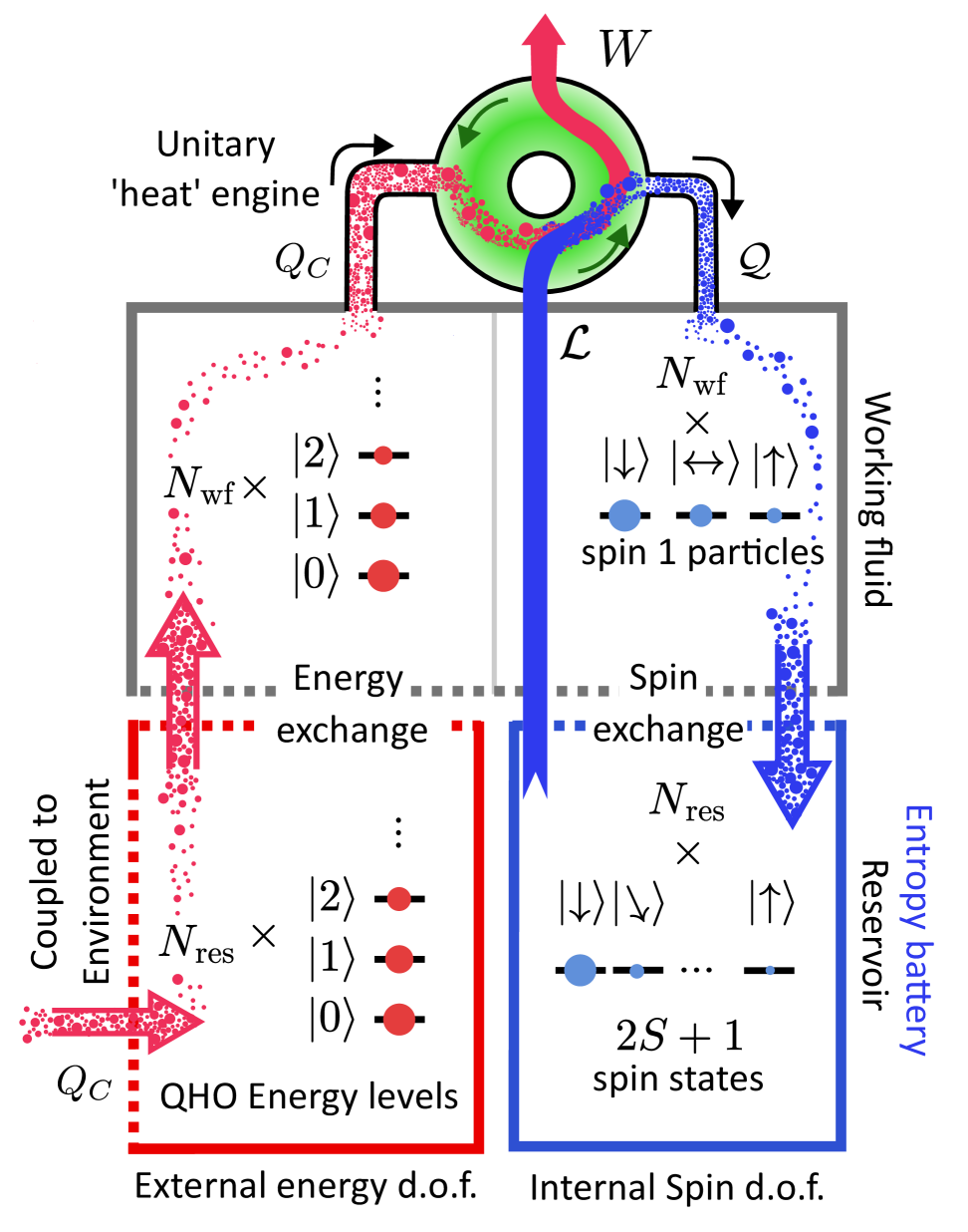
Figure 2: Schematic of the internal structure of the entropy battery. The device consists of two thermal, energy- and spin-coupled canonical ensembles: the working fluid and the reservoir, containing $N_{\text{wf}}$ and $N_{\text{res}}$ particles, respectively. Each ensemble has two mutually independent conserved quantities: the external energy modes of the quantum harmonic oscillators, labeled in the number basis $\ket{n}$, and internal spin states, labeled using the arrows $\ket{\uparrow}$. The particle distributions across these states are illustrated with circles and horizontal lines, where circle size represents the population at the respective temperatures. Since $N_{\text{res}}\gg N_{\text{wf}}$, the two ensembles equilibrate rapidly in both spin and energy, so that $T_{\text{res}}\approx T_{\text{wf}}$ and $\tau_{\text{res}}\approx\tau_{\text{wf}}$. The reservoir also couples thermally to an external hot environment, represented here by a canonical coupling in the bottom left, as in Fig.1. Particles in the reservoir have spin $S$, which sets the entropy capacity of the battery according to eqs.(2)–(2). In this schematic, incoherent properties (entropy) are represented with a spotted pattern, while coherent properties (information) are indicated by solid colors, illustrating the flow of entropy and information.

The working fluid consists of $N_{\text{wf}}$ spin-1 particles, and the reservoir contains $N_{\text{res}}$ spin-$S$ particles. These ensembles continuously thermalize in both spin and energy degrees of freedom via spin and energy exchange collisions, such that at any moment in time $T_{\text{wf}}\approx T_{\text{res}}$ and $\tau_{\text{wf}}\approx\tau_{\text{res}}$. Since $N_{\text{res}}\gg N_{\text{wf}}$, we approximate the total entropy of the entropy battery as arising primarily from the reservoir, $\mathbb{S}_{\text{battery}}=\mathbb{S}_{\text{wf}}+\mathbb{S}_{\text{res}}\approx\mathbb{S}_{\text{res}}$. The entropy capacity of the battery depends on the number of spin and energy states, as well as the number of particles, as dictated by eqs.(2)–(2). We now introduce the environment ensemble, which possesses only an energy degree of freedom. The joint environment, entropy battery system is assumed to be isolated from any ‘grander’ system, such that the composite system is closed, and there is a net zero change in entropy during the environment-battery thermalization process. As the environment couples to the entropy battery only via the energy degree of freedom, then the total change in entropy must be constrained by

$$\Delta\mathbb{S}_{\text{env}}(\tau_{\text{env}},\tau_{f})+\int_{\tau_{E,0}}^{\tau_{f}}\frac{1}{\tau_{E}}C_{V}d\tau_{E}+\int_{\tau_{s,0}}^{\tau_{f}}\frac{1}{\tau_{s}}C_{s}d\tau_{s}=0,$$ (24)

where $\tau_{E,0}$ and $\tau_{s,0}$ are the battery’s unitless energy and spin initial temperatures, and $\tau_{\text{env}}$ is the environments initial temperature, where $\tau_{\text{env}}>\tau_{E,0},\tau_{s,0}$. The unitless energetic temperature is $\tau_{E}=Tk_{B}/h\nu$, see Appendix E.3. $\tau_{f}$ is the unitless final temperature once equilibrium is reached, and is common across the conserved quantity waste baths as required by the zero’th law (2). The final temperature is dependent on the entropic responses $C_{s}/\tau$ of the environment, and the energy, spin waste baths of the battery.

II.2 Results

As we are interested in the theoretical potential of work extraction using the entropy battery, then we should use particle statistics that maximize the battery’s entropy capacity. At face value, it would appear as though distinguishable particles would provide the highest entropy capacity according to eq.(2), however, as will be discussed in §III, distinguishability implies non-interaction, making distinguishable particles unrealistic as our model (and real systems) require interactions between the canonical ensembles for entropy to transfer. The next best case is an ensemble of bosons. If both the environment and the battery have a large number of bosons, on the order of Avogadro’s number or more, then the waste responses $C_{s},C_{V}$ in the integrals of eq.(24) are approximately eq.(2), and the indefinite integrals $\int C_{s}/\tau d\tau$ evaluate to

$$\mathbb{S}_{\text{Boson}}= \sum_{j=1}^{d-1}\left(\frac{j}{2\tau}\frac{1}{\tanh(j/2\tau)}-\ln(\sinh(j/2\tau))\right)$$ (25)

$$-(d-1)\ln(2).$$

We use this expression to numerically solve for the final temperature by minimising $|\Delta\mathbb{S}|$ in eq.(24).

The final temperature is used in the analytic boson heat expression (2) to calculate the energetic heat transferred from the environment to the energy bath of the battery, and therefore the energetic work liberated. This represents the unitless work that is made available during a conventional heat engine cycle

$$W_{\text{conventional}}=|Q_{\text{env}}|-|Q_{\text{batt}}|.$$

The spin bath also absorbs entropy via the coupling heat engine, while simultaneously liberating heat energy in the battery as energetic work, at the cost of spin labor [10, 11]. Therefore, the total unitless energetic work of the entropy battery becomes

$$W_{\text{battery}}=|Q_{\text{env}}|-|Q_{\text{batt}}|+|\mathcal{Q}_{\text{batt}}|$$ (26)

where $\mathcal{Q}_{\text{batt}}$ is the spin therm absorbed by the battery’s spin waste bath. These heats and spin equivalents are all dependent on their respective waste responses $C_{s}$, and so the number of states each waste bath has access to. The energy baths of both the environment and the battery have in principal an infinite number of states as they are thermal motional states. We use a truncated energy state space ($d_{E}=400$) in our analysis without impacting accuracy.

The energy efficiency of the battery is

$$\eta_{\text{energy}}=\frac{W_{\text{battery}}}{|Q_{\text{env}}|}=1-\frac{|Q_{\text{batt}}|-|\mathcal{Q}_{\text{batt}}|}{|Q_{\text{env}}|},$$ (27)

and the results are shown in Fig.3 for varying initial battery temperatures. Fig.3 shows that once $d_{s}\geq 2$, the energy efficiency surpasses the Carnot limit. At 5 spin states, all initial temperatures considered reach close to $100\%$ energy efficiency. This occurs despite all waste baths being initially thermal states, without induced quantum coherence. Further, as the entropy transfer occurs adiabatically, the thermalization process must be endoreversible. The energy efficiency with 0 spin states follows $1-\sqrt{\tau_{1}/\tau_{2}}$, meaning our model represents the expected efficiency one would obtain when running a heat engine at maximum power [39, 40, 41]. See Appendix G.

Figure 3: Efficiency of energetic work extraction $\eta_{\text{energy}}$ for varying number of spin states per particle calculated using the entropy and heat equations (25) and (2). In these simulations we used $d_{\text{env}}=d_{\text{ens},E}=400$ without loss in accuracy. Also shown are 4 sets of initial temperatures for the ensembles energy and spin baths, with $\tau_{\text{batt}}=\tau_{E,0}=\tau_{s,0}$, while the environments initial temperature was set to $\tau_{\text{env}}=0.6$ for cases. These unitless temperatures were chosen as it would correspond to a temperature range between room temperature (300 K) for $\tau_{\text{batt}}=0.3$ on the low end and 600 K $\tau_{\text{env}}=0.6$ on the high end with a Debye cut off frequency of $21$ THz, which is a typical maximum frequency for metals [37]. These temperature ranges are typical in coal and nuclear power plants, and concentrated solar farms. As the number of spin states increases, the energy efficiency approaches 100%, with all initial conditions reaching approximately this limit at 5 states. This is well above the Carnot efficiency limit $\eta_{\text{Carnot}}=1-\tau_{\text{batt}}/\tau_{\text{env}}$ which is shown by the red bars when $d=0$, with values between 16%-50% for the varying initial ensemble temperatures.

II.3 Discussion

The Carnot limit sets the maximum efficiency achievable by a heat engine operating between two thermal reservoirs of different temperatures. As mentioned in the introduction, a common strategy in quantum heat engines to surpass this limit is to induce quantum coherence within the thermal bath, either via squeezed thermal states [26, 27, 28] or other induced coherences [29, 30, 31]. All of these devices operate below the generalized Carnot limit [32], therefore there is no real quantum advantage. In contrast, the entropy battery achieves super-Carnot efficiencies in large ensembles using only maximum entropy states, characterised by their unitless temperatures, demonstrating that this limit can be surpassed only when an energetically hot source is coupled to an ensemble with multiple conserved quantities via multiple unitary heat engines.

It must be re-iterated that this increase in energy efficiency comes at the cost of spin labor, with the generalized work of the battery being

$$\mathbb{W}=|Q_{\text{env}}|-|Q_{\text{batt}}|+|\mathcal{Q}_{\text{batt}}|-|\mathcal{L}|,$$

where $|\mathcal{L}|=|\mathcal{Q}_{\text{batt}}|$. The generalized efficiency of the battery when considering all resource costs therefore returns to the Carnot efficiency limit $\eta=1-|Q_{\text{batt}}|/|Q_{\text{env}}|$. Eq.(27) is therefore the energetic efficiency of the battery. If the initial preparation of spin labor within the battery requires energy, and if this energy cost is equal to the energy saved during the entropy transfer process in the unitary heat engine, then the entropy battery would not have an advantageous net energy efficiency. However, charging spin-polarized reservoirs does not necessarily require an energy input. Naturally occurring sources of spin coherence can instead be used to re-polarize the reservoir, analogously to how we currently use natural cold energetic baths to cool hot ensembles (from an entropic perspective). Consequently, the entropy battery now has an additional advantage: it extends the range of usable natural resources for energetic work extraction beyond energy alone. Further, the unitary heat engine that couples the external energy and internal spin degrees of freedom is controllable in the sense that it can be switched on/off. Combining this controllability with the assumed mutual independence of the spin degree of freedom, the state of ‘charge’ of the battery would remain approximately constant even in an energetically hot environment. This makes the entropy battery useful in applications that require such controllability, with it effectively performing the job of a conventional battery, all the while storing not energy, but information in the form of coherence when charged. Such a device could find broad applications, improving the energy efficiency of conventional batteries, power plants, and vehicles, while also enabling new methods of heat storage and refrigeration. Since the battery can, in principle, be charged using naturally occurring sources of quantum coherence in arbitrary conserved quantities, it opens the way to a future in which information itself becomes the only resource, a resource that can be controllably exchanged between conserved quantities as desired.

This paper focuses on an ideal scenario in which the battery-environment systems operate adiabatically. We briefly note the role of open-system effects here. Irreversibility may arise from the injection of entropy from an external source during thermalization, or from non-independent conserved quantities, such that the total entropy is non-extensive, $\mathbb{S}_{\text{battery}}<\mathbb{S}_{\text{energy}}+\mathbb{S}_{\text{spin}}$. Both reduce the effective entropy capacity of the battery, increasing the final temperature once energy and spin equilibrate across the conserved quantities and ensembles, and decreases the extractable work. Beyond improving isolation or enhancing the mutual independence of the conserved quantities, one could compensate for this loss by increasing the number of states, however that analysis is beyond the scope of this paper.

Another particular field that may apply the concepts developed in this paper is quantum error correction. The decoherence of a qubit over time can be described as a thermalization process with a thermal environment [42, 43], and as such, one can imagine that having access to another conserved quantity waste bath that is independent of the basis of measurement (the qubit) within a single physical system (the ion, superconductor etc.) would allow for the ‘re-direction’ of decoherence into the unused degree of freedom. If possible, this would slow the decoherence time of the measured qubit, potentially leading to less dependence on error correcting qubits. Actual implementation of such an error correcting technique is beyond the scope of this paper, however NMR algorithmic cooling [20, 19] bears some similarities in terms of using ancillary qubits (the spin states) for reversibly cooling the measurement qubit (the energy states).

III Maximizing entropy capacity

The analysis presented in this paper focuses on a single operating cycle, after which the environment is left cooler than its initial state, $\tau_{f}<\tau_{\text{env}}$. Repeated operation of the battery, assuming the environment is reset to its original temperature after each cycle, would allow continuous extraction of energetic work until the battery reaches the same dimensionless temperature as the now effectively isothermal environment, $\tau_{f}=\tau_{\text{env}}$. These extra cycles increase the amount of work extractable, where the number of cycles depends on the entropy capacity of the ensemble. Therefore, it is of interest to understand how one could maximize the battery’s entropy capacity. According to eqs.(2) and (2), one could increase the number of particles $N$ or states $d$, as either of these increases the number of microstates $\Omega$ and thus the entropy capacity. Another way would be to increase the number of independent conserved quantities. The dependence of the entropy capacity on these variables can be understood directly by application of the maximum entropy principle [6].

Consider a particle confined within a closed volume and isolated from any external interactions. Let the particle possess a total of $M$ conserved quantities, comprising both external (e.g., kinetic energy, momentum) and internal (e.g., spin, charge) degrees of freedom. For the $m^{\text{th}}$ unitless conserved quantity $A_{m}$, there are $d_{m}$ orthogonal eigenstates with eigenvalues $j$, labeled in the computational basis $j=0,1,2\dots,d_{m}-1$. Expanding the system to $N$ particles, we now introduce the definition of the macrostate, denoted $a_{j}$. Each particle can occupy a discrete state $j$, where there are $k_{j}$ such particles in the same state. The macrostate is then defined as $a_{j}=jk_{j}$, where $\sum_{j}k_{j}=N$. For any macrostate, there can be, in principal, many microstate. We denote these microstates $\Omega_{m}$, with $\Omega_{m}$ being the set of distinguishable configurations of particles across the $j$ states for the $m^{\text{th}}$ conserved quantity. In the most general case, permutations of individual particles add a combinatorial factor to the number of microstates that share the macrostate $a_{j}$. For example, if the particles are distinguishable, then there are $N!/(k_{0}!k_{1}!...)$ microstates for each $a_{j}$. In contrast, if the particles are indistinguishable then there are no such distinguishable permutations. Importantly, the Shannon entropy must be calculated as a sum over all distinguishable microstates

$$\mathbb{S}=-\sum_{\Omega}P(\Omega)\ln P(\Omega),$$ (28)

where $\Omega$ is the set of microstates across every conserved quantity.

The probability distribution that maximizes entropy, under the constraints of normalization $\sum_{\Omega}P(\Omega)=1$, Shannon entropy (28), and the $M$ total conserved quantities

$$\braket{A_{m}}= \sum_{\Omega}\left(\sum_{j=0}^{d-1}a_{j}(\Omega)\right)P(\Omega)$$ (29)

$$= \sum_{\Omega}a(\Omega)P(\Omega),$$

is [6]

$$P(\Omega)=\prod_{m=0}^{M}c_{m}P_{m}(\Omega,\gamma_{m})=\prod_{m=0}^{M}c_{m}e^{-\gamma_{m}a_{m}(\Omega)},$$ (30)

where $\gamma_{m}$ and $c_{m}$ are the Lagrange multiplier and normalization constant for the $m$^th conserved quantity. In this paper, all ensembles are treated as canonical, with no particle exchange and therefore no associated chemical potential. The ensemble normalization $\prod_{m}c_{m}=Z$ is,

$$Z=\sum_{\Omega}\prod_{m=0}^{M}e^{-\gamma_{m}a_{m}(\Omega)},$$

where $Z$ is the partition function. The entropy is therefore generally [6]

$$\mathbb{S}=\ln(Z)+\sum_{m=0}^{M}\gamma_{m}\braket{A_{m}}.$$

As defined, this entropy is sub-additive over the conserved quantities $\mathbb{S}\leq\sum_{m}\mathbb{S}_{m}$ as $Z$ is not necessarily separable over $m$, $Z\neq Z_{1}Z_{2}\dots Z_{M}$. However, if the conserved quantities are assumed to be mutually independent, then the total partition function factorises as $Z=\prod_{m}Z_{m}$, and the entropy becomes extensive, $\mathbb{S}=\sum_{m}\mathbb{S}_{m}$ where

$$\mathbb{S}_{m}=\ln(Z_{m})+\gamma_{m}\braket{A_{m}}.$$

Treating the conserved quantities as mutually independent also allows let’s us focus on each conserved quantity individually. For the conserved quantity $A_{m}$, the normalized probability distribution is

$$P(\Omega_{m},\gamma_{m})=\frac{e^{-\gamma_{m}a_{m}(\Omega_{m})}}{Z_{m}}$$ (31)

where

$$Z_{m}=\sum_{\Omega_{m}}e^{-\gamma_{m}a_{m}(\Omega_{m})}.$$

The microstates $\Omega_{m}$ of the $m$^th conserved quantity are now independent of the other conserved quantities. Therefore, mutual independence over the conserved quantities maximizes the ensembles entropy capacity. To further increase the entropy capacity, we are limited to increasing the number of microstates associated with the $M$ conserved quantities.

III.1 Distinguishability

Figure 4: An example entropy distribution over spin temperature for the different particle statistics, distinguishable, bosonic and fermionic with 7 states. In (a) and (b) we show example distributions with $N=4$ and $N=6$ particles respectively, illustrating how distinguishable and bosonic maximum entropies increase with $N$ without bound, while the fermionic maximum entropy decreases as saturation is approached $N=d$ where $\mathbb{S}_{\text{Fermi}}=0$ for all temperature. Maximum entropy is achieved once $\tau=\infty$, which we have labeled for the different ensemble statistics.

As shown in Fig.4, an ensemble of distinguishable particles achieves the largest entropy capacity. The partition function of such an ensemble is

$$Z_{\text{dist}}=\sum_{\mathbf{k}}\frac{N!}{k_{0}!k_{1}!...k_{d-1}!}\prod_{j=0}^{d-1}e^{-\gamma a_{j}},$$

where $\mathbf{k}=\{k_{0},k_{1},...,k_{d-1}\}$ specifies a configuration of the $k_{j}$ particles over the $j$ states. See Appendix B.1 for further details. This partition function is immediately factorizable for every one of the $N$ particles, since it is identically a multinomial expansion

$$Z_{\text{dist}}=\left(\sum_{j=0}^{d-1}e^{-\gamma j}\right)^{N}=Z^{N}.$$

This separability applies to the probability distribution (40)

$$P(\Omega,\gamma)=\left(\frac{e^{-\gamma a(\Omega)}}{Z}\right)^{N}=p(\gamma)^{N},$$

where $p(\gamma)$ is the single particle Boltzmann distribution. The entropy at infinite temperature $\gamma=0$ is therefore proportional to the number of particles

$$\mathbb{S}_{\text{max}}=N\ln(d).$$

A separable probability distribution and extensive entropy represents mutually independent entities. In the distinguishable particle ensemble, this mutual independence holds for each of the $N$ particles. Mutual independence therefore implies non-interaction, where interaction is defined generally as an event in which particles exchange a conserved quantity under the constraint of the relevant conservation law, or as a transfer of mutual information between particles. Consequently, distinguishable particles that maintain distinguishability at all times must be non-interacting. This has important implications for the entropy capacity of a realizable entropy battery. For unitary heat engines to operate, or for two canonical ensembles to thermalize, interactions between particles are required. For these reasons, distinguishable particles cannot be used in the entropy battery. Further discussion can be found in Appendix F.

The next best scenario is an ensemble of bosons. As discussed in Appendix B.2, unlike distinguishable particles, the probability distribution for an ensemble of bosons is non-separable down to the individual particles. Therefore, as a contrasting argument to the distinguishable particles, bosons must allow interaction, such that one cannot describe the particles as individuals after there becomes an exchange of information. The inseparability of the probability distributions after interaction is exactly how one would describe particle indistinguishability, and entanglement. The description we give implies that it is the mutual information upon interaction that ultimately determines a particles distinguishability. If the information is mutually exclusive then there remains a form of distinguishability, yet no interaction, but if the information is mutually dependent, then we lose distinguishability and there must have been an interaction. In this sense, what is ultimately indistinguishable upon interactions is the information that is encoded in the conserved quantities of the system. This is especially apparent when monitoring the mutual exchange of information between typically mutually independent conserved quantities like that used in the entropy battery. The exchange of generalized heats between conserved quantities is best understood in the context of information transfer.

Therefore, a system of bosons is the best case scenario for our model of the entropy battery, as they maximize entropy capacity while allowing information and entropy to be transferred between both the canonical ensembles of the battery and environment, and the independent conserved quantity.

IV Conclusion

From the perspective of information thermodynamics, an ensemble of particles with multiple, mutually independent conserved quantities exhibits an expanded entropy capacity. By applying unitary operations that couple these conserved quantities, this entropy capacity can be harnessed during work extraction, yielding energy efficiencies beyond the Carnot limit. We refer to such an ensemble as the entropy battery. We further justify treating spin angular momentum as an independent thermodynamic system by showing that, like energy, it obeys the laws of generalized thermodynamics, follows Bose-Einstein and Fermi-Dirac statistics, satisfies the fluctuation-dissipation and equipartition theorems (see Appendix B), and has analogous Einstein solid and Debye models of heat capacity. We also discuss the conditions under which particles are distinguishable (Appendices B.1 and F), concluding that distinguishable particles can exist only if they are non-interacting. Consequently, the apparent entropy capacity of such particles cannot be used for energetic work extraction via heat engines. This leads naturally to a generalization of indistinguishability in informational terms, independent of the specific conserved quantities or particles, and provides a conceptual understanding of the entropy battery as a device that transfers entropy through subsystem entanglement.

Appendix A Information Thermodynamics

In this section we derive, and present where assumed, the laws of spin thermodynamics, with these laws applying equally to arbitrary conserved quantities.

From the probability distribution in eq.(31), the Shannon entropy (28) of the spin component of the ensemble when mutually independent of any other degree of freedom is

$$\mathbb{S}=\ln(Z)+\gamma\braket{\bar{J}_{z}},$$ (32)

where $\braket{\bar{J_{z}}}=\braket{J_{z}}/\hbar$ and $\gamma$ are the unitless average angular momentum and spin Lagrange multipliers respectively. We have removed the ‘$m$’ label for brevity. From eq.(32), we show a familiar, and generally known relation

$$\frac{\partial\mathbb{S}}{\partial\braket{\bar{J}_{z}}}=\gamma$$ (33)

[7], which is directly analogous to the thermodynamic relation of energy and entropy [44]

$$\frac{\partial\mathbb{S}}{\partial\braket{E}}=\frac{1}{T}.$$ (34)

This leads to the interpretation of the Lagrange multiplier of the average spin angular momentum constraint, $\gamma$, as the inverse spin temperature $\tau=\frac{1}{\gamma}$ [12]. From eq.(31), we also obtain expressions of average angular momentum in terms of the partition function

$$\braket{\bar{J}_{z}}=\tau^{2}\frac{\partial}{\partial\tau}\ln(Z)=-\frac{\partial}{\partial\gamma}\ln(Z),$$ (35)

which is analogous to the expression of average energy

$$\braket{E}=-\frac{\partial}{\partial\beta}\ln(Z)$$

where $\beta=k_{B}T$ is the energy Lagrange multiplier [6, 7]. Negative spin temperatures appear due to having finite eigenstates, which is a phenomena also found in energetic systems with finite energy eigenstates [45, 46].

Showing the zero’th and third laws of spin thermodynamics is straightforward from here. Consider a spin ensemble with many particles, that is also in a state of maximum entropy such that it’s probability distribution is described by eq.(31) with spin temperature $\tau_{1}$. Take another similar spin system that is independently at a state of maximum entropy, with spin temperature $\tau_{2}$, where initially $\tau_{1}\neq\tau_{2}$. Upon spin exchange contact without particle exchange, the ensembles evolve in what can be considered a spin thermalization process. By the first law of generalized thermodynamics, the net change in spin between the ensembles is 0

$$\delta\braket{\bar{J}_{z,1}}=-\delta\braket{\bar{J}_{z,2}}.$$ (36)

Since this is a closed system, then the net change in entropy during thermalization must also be 0,

$$\delta\mathbb{S}_{1} =-\delta\mathbb{S}_{2}.$$ (37)

Eq.(37) would imply that in principal the system is reversible as it follows Liouvillian trajectories, which are deterministic. Eq.(37) is the second law of spin thermodynamics for freely evolving isolated systems.

As these two ensembles are initially independent, then both the total spin angular momentum and total entropy of each ensemble add extensively. Changes in a systems spin angular momentum therefore has a corresponding change in entropy, and this is balanced by an equivalent change in the other system. During the spin thermalization process these systems will exchange spin and entropy deterministically up until the ratio $\delta J_{z}/\delta S$ for the two systems are equal, which comes from the division of eqs.(36) and (37)

$$\frac{\delta\braket{\bar{J}_{z,1}}}{\delta\mathbb{S}_{1}}=\frac{\delta\braket{\bar{J}_{z,2}}}{\delta\mathbb{S}_{2}}.$$

For ensembles with large $N$, the fluctuations of spin angular momentum and entropy between the baths become vanishingly small with respect to the average equilibrium values, as the relative variation scales with $1/\sqrt{N}$ [36]. We can therefore approximate the small changes as an infinitesimal, and make use of the result in eq.(33) to show that this can only be true if

$$\tau_{1}=\tau_{2},$$ (38)

meaning the two systems will reach spin exchange equilibrium when $\tau_{1}=\tau_{2}$. This is the zero’th law of spin thermodynamics.

Finally, the entropy of this system will approach 0 as the spin temperature approaches 0. This can be shown explicitly using the expression of the probability distribution (31). As $\tau\rightarrow 0$

$$P(\Omega)=\begin{cases}0,&k_{0}\text{ or }k_{d-1}\neq N\\ 1,&k_{0}\text{ or }k_{d-1}=N,\end{cases}$$

which is to say the spin system becomes maximally polarized. In this case, the entropy (32) is 0 for all microstates, and so the total entropy is 0. This is the third law of spin thermodynamics.

Aside from the laws of thermodynamics applying to spin angular momentum, Vaccaro et. al. have explored the concepts of spin ‘heat’ and spin ‘work’ , renamed spin therm $\mathcal{Q}$ and spin labor $\mathcal{L}$ respectively [11, 10]. It was shown that heat engines operating with spin systems can be written in terms of these analogous thermodynamic properties.

We conclude that spin, when treated as an independent conserved quantity, follows the same laws of thermodynamics as energy. It can be expected that any application of thermodynamics, such as heat engines, would also work within spin systems. In the case of spin heat engines that operate between two spin reservoirs, the ‘work’ that is extracted will be in the form of coherent spin angular momentum, or spin labor $\mathcal{L}$. However, unitary coupling of the energy basis to the spin basis within a single system can allow for the extraction of energetic work [11, 24]. As spin follows the laws of thermodynamics, then thermodynamics is clearly not a theory of only energy and heat. With this section applying to arbitrary unitless mutually independent conserved quantity $A_{m}$ by substitution, then a general interpretation of these results is that thermodynamics is fundamentally an information theory.

Appendix B Ensemble Probability distributions

B.1 Distinguishable particles

An ensemble of labeled particles are, by definition, distinguishable. The exact labeling scheme one might use is discussed in Appendix F. For this ensemble, the number of microstates $\Omega$ increases as permutations of the particles that are in a particular configuration $\mathbf{k}=\{k_{0},k_{1},...k_{d-1}\}$ constitute new microstates. The multiplicity of state configurations $g(\mathbf{k})$ that result in the same macrostate $a(\Omega)$ if all particles are distinguishable from one another is a multinomial

$$g_{\text{dist}}(\mathbf{k})=\begin{pmatrix}N\\ k_{0},k_{1},...k_{d-1}\end{pmatrix}=\begin{pmatrix}N\\ \mathbf{k}\end{pmatrix}.$$

This multiplicity is the same used by Bernoulli and Laplace for distinguishable particles [47]. The partition function can then be represented as

$$Z_{\text{dist}}={\sum_{\mathbf{k}}}\begin{pmatrix}N\\ \mathbf{k}\end{pmatrix}\prod_{j=0}^{d-1}e^{-\gamma m_{j}k_{j}}$$

which is a multinomial expansion of the variables $e^{-\gamma m_{j}}$, and so the partition function can be simplified to

$$Z_{\text{dist}}=\left(\sum_{j=0}^{d-1}e^{-\gamma m_{j}}\right)^{N}=Z^{N}.$$ (39)

The partition function for distinguishable particles is therefore separable into a product of the per particle partition function $Z=\sum_{j=0}^{d-1}e^{-\gamma m_{j}}$. This separability applies also to the probability distribution. From eq.(31),

$$P(\Omega) =\frac{e^{-\gamma\sum_{j=0}^{d-1}m_{j}k_{j}}}{Z^{N}}$$

$$P(\Omega) =\left(\frac{e^{-\gamma m_{0}k_{0}}}{Z^{k_{0}}}\right)\left(\frac{e^{-\gamma m_{1}k_{1}}}{Z^{k_{1}}}\right)\dots$$

$$=\prod_{j=0}^{d-1}p(j)^{k_{j}}=p(j)^{N}$$ (40)

where $p(j)=e^{-\gamma m_{j}}/Z$ is the Boltzmann distribution for a single particle in state $j$. Eq.(40) is separable down to the individual particles.

The separability of the particles’ probability distributions is significant, as probability theory requires that such particles be mutually independent. Each particle must act as an independent entity, unable to influence the outcomes of the others. Consequently, particles can only be considered distinguishable if they are non-interacting. This is discussed further in Appendix F.

B.1.1 Polarization, spin temperature relation

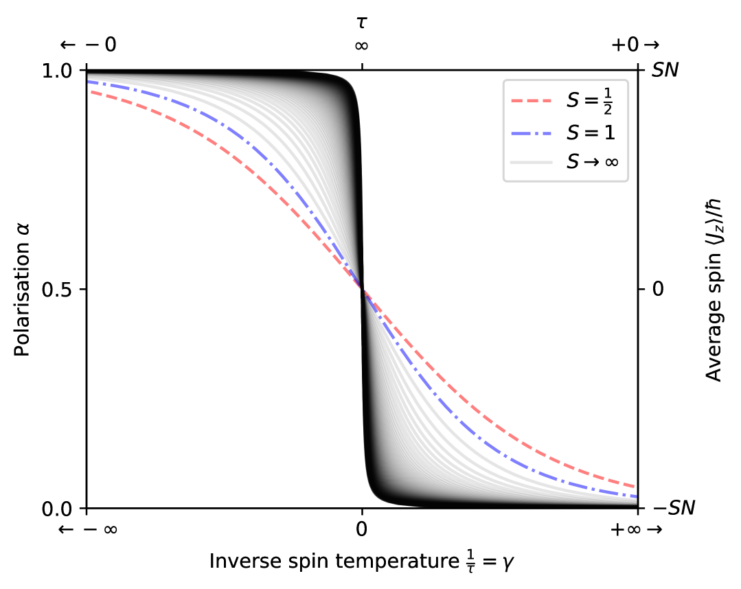
Figure 5: Mapping of spin temperature $\tau$ to polarization, eq.(42), for different ensembles of distinguishable particles with per particle spins $S$. This plot shows up to $S=200$, but trends towards a steepening slope around $\gamma=0$, where in the limit of $S\rightarrow\infty$ one would expect a step function centred at $\gamma=0$

It is convenient to re-express the spin temperature $\tau$ in terms of the spin-polarization $\alpha$, thus providing a mapping to the macroscopic observable $J_{z}$. From eq.(35)

$$\left(2\alpha S-S\right)N =-\frac{\partial}{\partial\gamma}\ln\left(Z_{\text{dist}}\right)$$

$$2\alpha S-S =-\frac{\partial}{\partial\gamma}\ln\left(\sum_{j=0}^{d-1}e^{-\gamma m_{j}}\right)$$

where $\braket{\bar{J}_{z}}=(2\alpha-1)SN$. From this we obtain a polynomial

$$2\alpha S-S =\frac{\sum_{j=0}^{d-1}m_{j}e^{-\gamma m_{j}}}{\sum_{i=0}^{d-1}e^{-\gamma m_{j}}}$$

$$0 =\sum_{j=0}^{d-1}e^{-\gamma m_{j}}(2\alpha S-m_{j}-S).$$ (41)

Since spin angular momentum is quantised with evenly spaced spin states, then $m_{j}=j-S$ and eq.(41) can be written as

$$0=\sum_{j=0}^{d-1}e^{-\gamma j}(2\alpha S-j).$$

This polynomial is of the $d-1=2S$ order for the variable $e^{-\gamma}$ with coefficients $2\alpha S-j$. Solving the root provides the mapping of spin temperature to polarization

$$\tau=\ln\left(\frac{1}{f(\alpha)}\right)^{-1},$$

where $f(\alpha)$ is the real positive root of the polynomial $\sum_{j=0}^{d-1}x^{j}(2\alpha-j)$. The roots must be real and positive as $\tau$ must be real, and $\ln(x)$ requires positive arguments to compute.

Some example solutions that can be analytically expressed include the $S=\frac{1}{2}$ (linear) and $S=1$ (quadratic) systems

$$S=\frac{1}{2}: \quad\tau=\ln\left(\frac{1-\alpha}{\alpha}\right)^{-1}$$ (42)

$$S=1: \quad\tau=\ln\left(\frac{4(1-\alpha)}{(2\alpha-1)+\sqrt{-12\alpha^{2}+12\alpha+1}}\right)^{-1}$$

Higher-order solutions are solved numerically and are presented in Fig.5. These relations of temperature to polarization are equivalent to expressions found in the equipartition theorem for discrete systems [48], with our work generalizing to an arbitrary number of orthogonal states $d=2S+1$ for distinguishable particles.

B.2 Bosons

For a canonical ensemble of indistinguishable bosons, any permutations on the configuration of particles $\mathbf{k}$ is not itself a new microstate like that for distinguishable particles. Therefore, the multiplicity $g(\mathbf{k})=1$ for all configurations of $\mathbf{k}$, and the microstates $\Omega=\mathbf{k}$. The probability distribution from eq.(31) now becomes

$$P_{\text{Boson}}(\mathbf{k})=\frac{e^{-\gamma\sum_{j=0}^{d-1}m_{j}k_{j}}}{Z_{\text{Boson}}},$$ (43)

where

$$Z_{\text{Boson}}=\sum_{\mathbf{k}}e^{-\gamma\sum_{j=0}^{d-1}m_{j}k_{j}}.$$ (44)

By changing the index from the particle configuration $\mathbf{k}$ to the macrostate $a(\mathbf{k})=\sum_{j=0}^{d-1}m_{j}k_{j}$, we show that spin bosons follow Bose-Einstein statistics [35]. The macrostate index $a(\mathbf{k})$ ranges from $-SN$ to $SN$, which we can shift to the computational macrostate $m=a(\mathbf{k})+SN=\sum_{j=0}^{d-1}jk_{j}$ without affecting the distribution. The multiplicity using this index is derived in Appendix C, and is explicitly the coefficient of the $[x^{m}]$^th term of a Gaussian binomial,

$$g_{\text{Boson}}(m)=[x^{m}]\begin{pmatrix}N+d-1\\ d-1\end{pmatrix}_{x}.$$ (45)

This shows that the partition function is

$$Z_{\text{Boson}}=\begin{pmatrix}N+d-1\\ d-1\end{pmatrix}_{p}:\quad p=e^{-\gamma}.$$ (46)

Both eqs.(44) and (46) are equivalent, however they do not automatically allow for separable distributions like that for the distinguishable particles. These expressions obey Bose-Einstein statistics, with $\sum_{m}g_{\text{Boson}}={}^{N+d-1}C_{N}$ being the multiplicity used by Bose for an ensemble of bosons in the energy basis [35]. Going further, we explicitly show that spin bosons follow the Bose–Einstein distribution in the limit of an infinite number of particles. The partition function (46) can then be expressed as a generating function

$$Z_{\text{Boson}} =[t^{N}]\sum_{k_{j}=0}^{\infty}\begin{pmatrix}k_{j}+d-1\\ d-1\end{pmatrix}_{e^{-\gamma}}t^{k_{j}}$$ (47)

$$=[t^{N}]\prod_{j=0}^{d-1}\frac{1}{1-te^{-\gamma m_{j}}},$$ (48)

where $[t^{N}]$ is a selection variable, used to select the polynomials of $t$ that correspond to $N$ particles, and eq.(48) is an identity from Newton’s generalized binomial theorem. Eq.(48) demonstrates that, in the infinite-particle limit, the boson partition function becomes separable over the macrostates

$$Z_{\text{Boson}}=[t^{N}]\prod_{j=0}^{d-1}z_{\text{Boson}}(j,t).$$ (49)

As in the distinguishable case (Appendix B.1), this implies that in the infinite-particle limit, the probability distributions of each state $j$ are mutually independent, though the particles themselves are not. The state dependent probability distribution is

$$P(j)=\frac{e^{-\gamma m_{j}k_{j}}}{z(j)},$$

where

$$z(j)=\frac{1}{1-e^{\gamma m_{j}}}=\sum_{k_{j}=0}^{\infty}e^{-\gamma m_{j}k_{j}}.$$

The selection variable $t$ was removed as the states $j$ are now effectively mutually independent grand canonical ensembles, and we are no longer considering a finite system. The average occupation of particles in state $j$ is then

$$\braket{n_{j}} =\sum_{k_{j}=0}^{\infty}k_{j}P(j)=\frac{1}{z(j)}\sum_{n=0}^{\infty}k_{j}e^{-k_{j}\gamma(j-S)}$$

$$=\frac{1}{z(j)\gamma}\left(\frac{\partial}{\partial S}z(j)\right)$$

$$=\frac{1}{e^{\gamma m_{j}}-1},$$ (50)

where we used $m_{j}=j-S$. Eq.(50) represents the Bose–Einstein distribution [35] in the spin degree of freedom. The separability of the probability distributions occurs only in the limit of an infinite number of particles, and only separable over the states. Since this separability does not apply to individual particles, the particles themselves are not mutually independent and bosons must allow interaction.

B.3 Fermions

Fermionic systems modify the ensemble statistics further due to the antisymmetric nature of particle exchange, which gives rise to the Pauli exclusion principle [49]. We can no longer assume that an arbitrary number of particles may occupy the same spin state, as this would violate the exclusion principle if the particles also shared identical values in all other conserved quantities.

Assuming the particles occupy identical states across all other degrees of freedom, the system can contain at most $N=d$ particles, corresponding to one particle per spin state. Therefore, this system is constrained by

$$\sum_{j=0}^{d-1}k_{j}=N\leq d;\quad k_{j}\in\{0,1\}.$$ (51)

The set of microstates $\Omega$ is then $\Omega=\mathbf{k}_{\text{Fermi}}=\{k_{j}\in\{0,1\}:k_{0},k_{1},...,k_{d-1}\}$, and the probability distribution is

$$P(\mathbf{k}_{\text{Fermi}})=\frac{e^{-\gamma\sum_{j=0}^{d-1}jk_{j}}}{Z_{\text{Fermi}}}.$$

where

$$Z_{\text{Fermi}}=\sum_{\mathbf{k}_{\text{Fermi}}}e^{-\gamma\sum_{j=0}^{d-1}jk_{j}}$$

As in the bosonic case, by changing to the macrostate index $m$, we can explicitly show that spin fermions follow Fermi–Dirac statistics. The multiplicity of the macrostate $m=a(\mathbf{k}_{\text{fermi}})+SN=\sum_{j=0}^{d-1}jk_{j}$ is calculated using the generating function

$$g_{\text{Fermi}}(m)=[t^{N}x^{m}]\prod_{j=0}^{d-1}(1+tx^{j})$$

where $[t^{N}x^{m}]$ selects the polynomial terms that correspondingly have $N$ atoms with macrostate index $m$. The fermion partition function using the $m$ index is then

$$Z_{\text{Fermi}}=[t^{N}]\prod_{j=0}^{d-1}(1+te^{-\gamma j})=[t^{N}]\prod_{j=0}^{d-1}z_{\text{Fermi}}(j,t).$$ (52)

The fermion partition function is thus separable over the macrostates $m$, allowing each state to be treated as a mutually independent grand canonical ensemble, where

$$z_{\text{Fermi}}(j,t) =\sum_{n=0}^{1}t^{n}e^{-n\gamma j}=1+te^{-\gamma j}.$$

The state probability distribution with only 0 or 1 particles in state $j$ is then

$$P(j,t)=\frac{e^{-\gamma jk_{j}}}{1+te^{-\gamma j}}$$

and

$$P(\mathbf{k}_{\text{Fermi}})=[t^{N}]\prod_{j=0}^{d-1}P(j,t),$$

showing directly that the states $j$ are mutually independent. The average number of particles in state $j$ then becomes

$$\braket{n_{j}}=\sum_{k_{j}=0}^{1}k_{j}P(j)=\frac{1}{e^{\gamma j}+1}$$

which is the Fermi-Dirac distribution [50]. We have removed the selection variable $t$, as this expression does not impose a constraint on the total particle number $N$. The separability of the probability distribution across the states $j$ allows each state to be treated as mutually independent. However, as in the bosonic case, the particles themselves cannot be considered mutually independent. Consequently, from a statistical perspective, fermions also permit interaction between particles. Finally, in the limit that $\tau\rightarrow\infty$, eq.(52) becomes

$$Z_{\text{Fermi}}=\begin{pmatrix}d\\ N\end{pmatrix}.$$

The entropy of distinguishable, bosonic and fermionic ensembles is presented in Fig.4, showing that an ensemble of distinguishable particles can store far more entropy than bosonic and fermionic ensembles. What we hope is clear is that the statistics and probability distributions for energetic systems apply equally to any mutually independent conserved quantity, like spin angular momentum.

Appendix C Multiplicity of Boson spin states

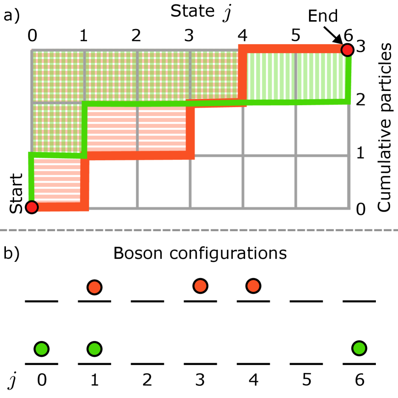
Figure 6: Boson microstates (b) represented using the $N\times d$ grid problem (a), where the grid dimensions correspond to the total particle number $N$ and the number of states per particle $d$. The grid problem counts the number of unique paths starting from the “Start” corner and ending at the “End” corner, restricted to upward and rightward moves, that result in the same area above the path. In (a) two example paths are shown, with (b) displaying the corresponding boson configurations in the $j$ states. The shaded area represents the macrostate, with areas of 7 and 8 for the green and red paths, respectively, corresponding to the correct macrostates for the particle distributions depicted in (b).

The number of configurations of indistinguishable bosons that yield the same total spin angular momentum can be reformulated as a combinatorial problem: counting the number of unique paths on an $N\times d$ grid, starting from the bottom-left corner and ending at the top-right corner, with movement restricted to upward and rightward steps, as illustrated in Fig.6. The grid represents $N$ particles distributed among $d$ states, and the area of the grid above the path taken represents the macrostate $m(\mathbf{k})=\sum_{j=0}^{d-1}jk_{j}$.

The question then becomes ‘how many unique paths result in the same area’? Answering this question is equivalent to determining how many configurations of indistinguishable particles yield the same macrostate. The solution is a generating function of the Gaussian binomial [51],

$$\text{Comb}=[q^{m}]\begin{pmatrix}N+d-1\\ d-1\end{pmatrix}_{q}$$

where $m=m(\mathbf{k})\in\{0,1,2\dots(d-1)N\}$. This can then be interpreted as simply the multiplicity of microstates $g(m)$ for boson when indexed over the macrostates. We can then use this to derive the boson partition function in terms of the macrostates,

$$Z_{\text{Boson}}=\begin{pmatrix}N+d-1\\ d-1\end{pmatrix}_{q}:\quad q=e^{-\gamma}.$$

Appendix D Waste and Entropic responses

In thermodynamics, the heat capacity is commonly defined as the amount of heat required to raise the temperature of a system by one unit. Equivalently, it can be interpreted as the amount of waste energy (i.e., heat) that the system can store for a given change in temperature. Heat capacity is defined as

$$C_{V}=\left(\frac{\partial U}{\partial T}\right)_{V}$$

for constant volume $V$ [52]. It can also be expressed in terms of the system’s entropy

$$C_{V}=T\left(\frac{\partial\mathbb{S}}{\partial T}\right)_{V}.$$

We can define an analogous quantity for the spin degree of freedom. Since spin angular momentum depends only on the spin temperature $\tau$ and has no analog of volume or pressure, we define the “spin therm capacity” as

$$C_{s}=\frac{d\braket{\bar{J}_{z}}}{d\tau}.$$ (53)

Using eq.(2), we can equivalently write

$$C_{s}=\tau\frac{d\mathbb{S}}{d\tau}$$ (54)

where we can interpret

$$\frac{1}{\tau}C_{s}=\frac{d\mathbb{S}}{d\tau}$$ (55)

as the amount of entropy the system can store per unit change in spin temperature. It should be clear that any mutually independent conserved quantity possesses an analogous heat capacity. It is therefore natural to define $C_{s}/\tau$ as the entropic response of the ensemble, a quantity that applies generally to any independent conserved variable, such as spin or energy. $C_{s}$ should be interpreted as the waste response of the ensemble, specific to the conserved quantity in question and associated with an analogous “heat” or the loss of usefulness of that conserved quantity. Re-naming $C_{s}$ from what is conventionally the ‘heat’ capacity emphasizes that $C_{s}$ is not a measure of capacity per se, but rather quantifies the absorbed ‘waste’ in response to a change in temperature. This is especially evident when considering the expression of the distinguishable waste response from table 2. The proportionality to the variance of the conserved quantity is a phenomena found generally in the fluctuation-dissipation theorem [36], where $C_{s}$ is the response function. Renaming the heat capacity to the waste response is therefore justified from this perspective. Eqs.(53) and (55) are presented as alternate, yet equivalent interpretations of a systems ability to store waste, both from a physical and an entropic perspective. These two equations allow for us to interpret heat engines in §II as being machines that either filter conserved quantities by separating the ‘heat’ from the ‘work’, or machines that merely transport entropy and information between the heat baths, with these interpretation also applying to the operation of conventional energy heat engine. The information interpretation of the heat engine is general, and leads naturally to concepts involving information transfer between ‘waste’ baths of different conserved quantities, such as spin and energy.

$C_{s}$ can be expressed generally using eqs.(2) and (2)

$$C_{s}=2\tau\left(\frac{d}{d\tau}\ln(Z)\right)+\tau^{2}\left(\frac{d^{2}}{d\tau^{2}}\ln(Z)\right),$$ (56)

showing a dependence only on the partition function. For an ensemble of bosons with infinite particles, where we can treat each state as independent Grand canonical ensembles (49), then $C_{s}$ is analytically the specific heat capacity of an Einstein-solid [37] when $S=\frac{1}{2}$. The waste response is derived for arbitrary spin system composed of bosons and distinguishable particles in Appendix E.1-E.3, with the results summarised in Table.2. These results are also presented in Fig.7, along with the unitless, per degree of freedom Debye and Einstein-solid models of specific heat capacity.

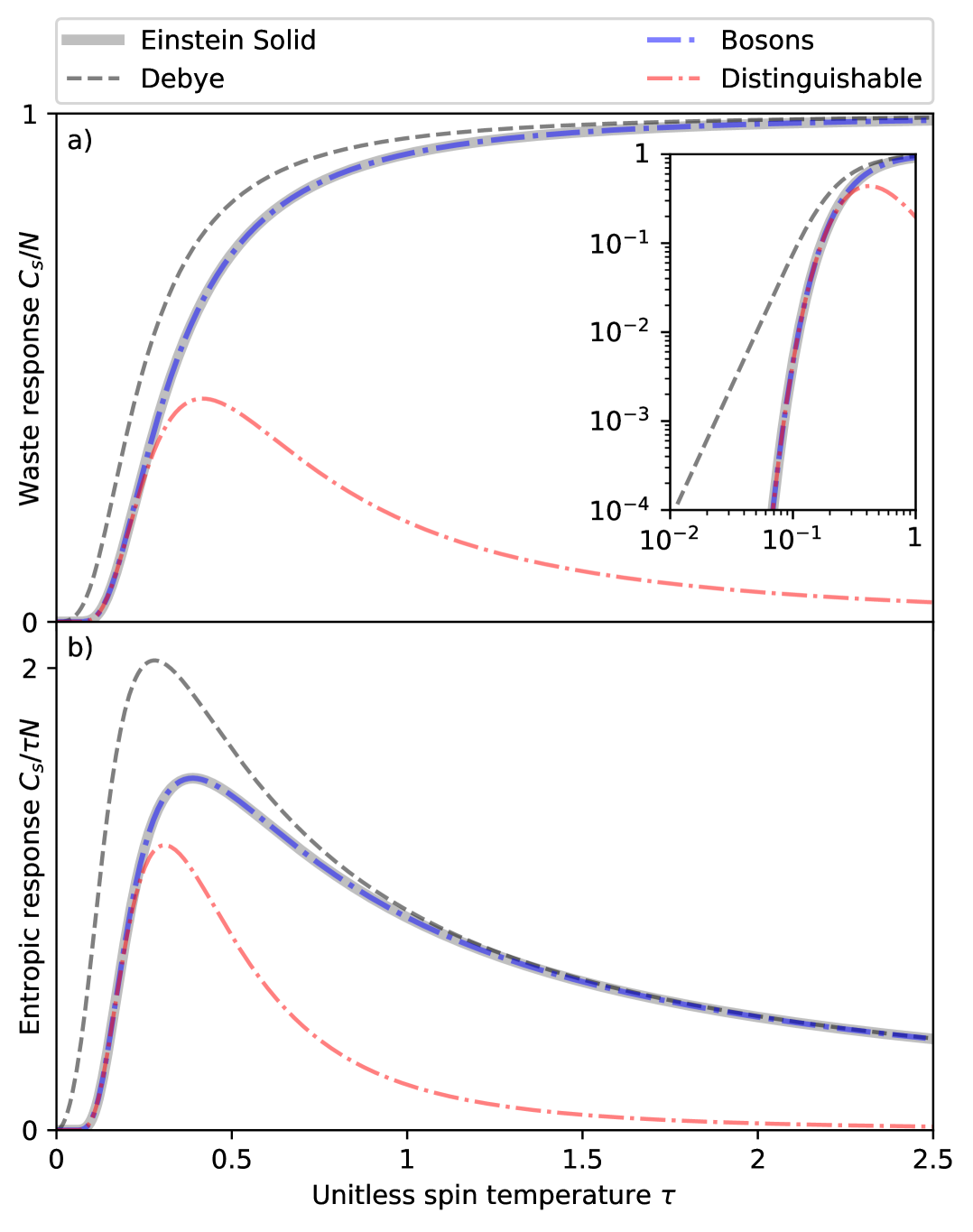
Figure 7: (a) The waste response - colloquially the specific heat capacity - and (b) the entropic response for bosonic and distinguishable ensembles. Also shown are the Einstein solid and Debye models of specific heat capacity for a single degree of freedom [37]. For all curves $S=1/2$ and the expressions from Table.2 were used. The Debye model provides the most accurate description of energetic heat capacity across all temperatures, as it accounts for low-temperature phonon effects commonly observed in metals. The inset in (a) shows the deviation between the Einstein and Debye models in the low-temperature limit and is included for comparison with Fig. 1 of [53].

The system’s entropy capacity, $\mathbb{S}_{\text{max}}$, defined as the maximum entropy the system can store, is given by the integral of the entropic response with respect to temperature. From eq.(55)

$$\mathbb{S}_{\max}=\int_{0}^{\mathbb{S}_{\max}}d\mathbb{S}=\int_{0}^{\infty}C_{s}\frac{1}{\tau}d\tau.$$ (57)

The waste capacity, defined as the maximum unitless “heat” that the ensemble can absorb, can be calculated similarly using eq.(56).

$$\mathcal{Q}_{\text{max}}=\int_{-SN}^{0}d\braket{\bar{J}_{z}}=\int_{0}^{\infty}C_{s}d\tau$$

Although trivial in their derivation, these two equations should be understood as representing two distinct ways in which an ensemble can store waste. In one representation, the ensemble stores entropy, corresponding to the lack of information about the system’s distribution across its microstates. In the other, it stores the “disordered” physical quantity, heat, or more generally, waste. Evaluating eq.(57), we find that the entropy capacity is

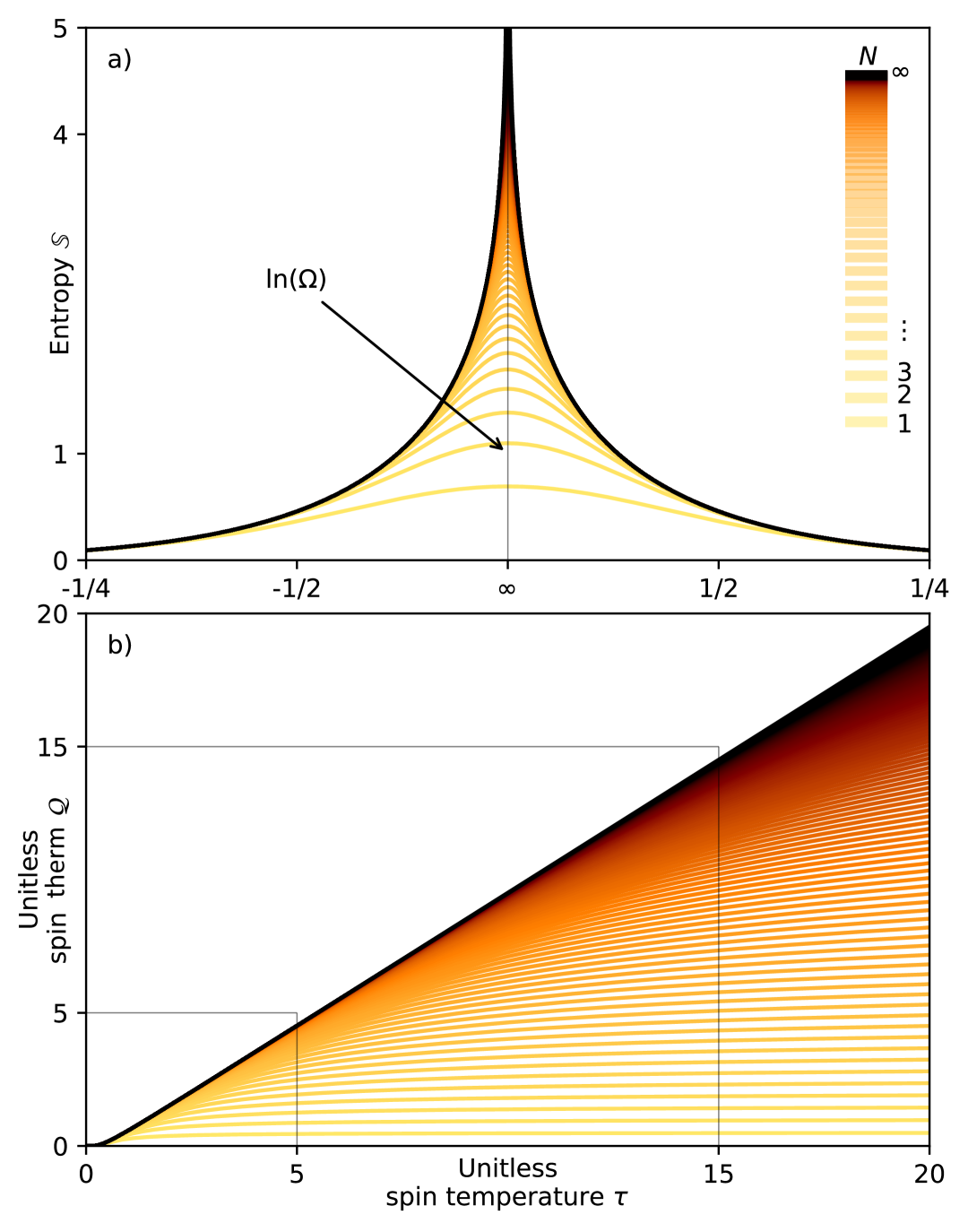
Figure 8: (a) The bosonic entropy and (b) spin therm for varying spin temperature $\tau$ with $S=1/2$. The coloured lines show the numerical entropy and heat for increasing $N$ from $N=1$, calculated using the waste response from eq.(56), $Z_{\text{Boson}}$ from eq.(46) and integrating eqs.(53) and (55). In black in both subplots is the analytic entropy and heat from (25) and (2). In (a) we labeled the maximum entropy when $\tau=\infty$ using the grey vertical line, and in (b) we make it clear how in the large $\tau$ limit with large $N$ that $\mathcal{Q}\propto\tau$. (b) also shows the large $\tau$ limit of heat with finite $N$ of $\mathcal{Q}_{\text{max}}=SN$ from eq.(59).

$$\mathbb{S}_{\text{max}}=\lim_{\tau\rightarrow\infty}\mathbb{S}=\ln\left(\sum_{\Omega}1\right)=\ln(\Omega).$$ (58)

$\mathbb{S}_{\text{max}}$ is therefore determined by the total number of microstates. This is Boltzmann’s definition of entropy for energy systems $\mathbb{S}/k_{B}=\ln(\Omega)$ [54]. The entropy for distinguishable particles is extensive with the number of particles, as $|\Omega|=d^{N}$. However it is non-extensive for indistinguishable particles. The waste capacity or maximum spin therm the spin ensemble can absorb is

$$\mathcal{Q}_{\text{max}}=SN=\frac{d-1}{2}N$$ (59)

which is extensive in the number of particles, regardless of whether they are distinguishable or indistinguishable.

Finally, in the infinite $N$ limit the entropy and spin therm for bosons becomes eqs.(25) and (2). The boson spin therm is proportional to $\tau$ in the high temperature limit, as the Taylor expansion of $\coth(1/x)\approx x$ for $x\gg 0$, which re-derives the usual heat expression $\mathcal{Q}\propto\tau$ used in, for example, deriving the standard Carnot efficiency limit $\eta=1-\tau_{c}/\tau_{h}$. Eqs.(25) and (2) are presented graphically in Fig.8.

Appendix E Analytic waste response

E.1 Distinguishable particles

From eq.(39), the partition function for an ensemble of $N$ distinguishable particles with $d$ states per particle is

$$Z_{\text{dist}}=\left(\sum_{j=0}^{d-1}e^{-j/\tau}\right)^{N}=Z^{N}$$

where we have written the distinguishable partition function in terms of the per particle partition function $Z$. The derivative of $\ln(Z_{\text{dist}})$ is

$$\frac{d}{d\tau}\ln(Z_{\text{dist}})=\frac{N\sum_{j=0}^{d-1}je^{-j/\tau}}{\tau^{2}\sum_{j=0}^{d-1}e^{-j/\tau}}=\frac{N}{\tau^{2}}\braket{j(\tau)}$$

where we have identified the average spin state index $\braket{j(\tau)}$ as being the weighted sum of the states

$$\braket{j(\tau)}=\sum_{j=0}^{d-1}jP(j,\tau)$$

for probability $P(j,\tau)=e^{-j/\tau}/Z$, and $Z=\sum_{j=0}^{d-1}e^{-j/\tau}$. Note also that $\braket{j}N=\braket{\bar{J}_{z}}+SN$. The second derivative is then

$$\frac{d}{d\tau}\frac{N}{\tau^{2}}\braket{j(\tau)}=-\frac{2N}{\tau^{2}}\braket{j(\tau)}+\frac{N}{\tau^{4}}\left(\braket{j(\tau)^{2}}-\braket{j(\tau)}^{2}\right).$$

We can identify the variance in $j$, $\text{Var}(j(\tau))=\braket{j(\tau)^{2}}-\braket{j(\tau)}^{2}$, and therefore derive the final form of the waste response

$$C_{s}=\frac{N}{\tau^{2}}\text{Var}(j(\tau))$$

It can be shown by using

$$\braket{\bar{J}_{z}}=\sum_{j=0}^{d-1}m_{j}P(j)=\sum_{j=0}^{d-1}m_{j}\frac{e^{-j/\tau}}{Z}$$

that

$$\text{Var}(\bar{J}_{z}(\tau))=\text{Var}(j(\tau)).$$

This gives us the final form of the per particle waste response for distinguishable information

$$\frac{C_{s}}{N}=\frac{1}{\tau^{2}}\text{Var}(\bar{J}_{z}(\tau))$$

E.2 Bosons

From appendix B.2, the partition function for an ensemble of $N$ boson with $d$ states per particle is

$$Z_{\text{Boson}}=\begin{pmatrix}N+d-1\\ d-1\end{pmatrix}_{p}:\quad p=e^{-\gamma}$$

In the limit that $N\rightarrow\infty$, this becomes

$$Z_{\text{Boson}}=\prod_{j=1}^{d-1}\frac{1}{1-e^{-j\gamma}}$$

from Newton’s generalized binomial theorem. We can exploit the fact that the partition function may be multiplied by any constant without altering the normalized probability distribution or the waste response. The choice of constant is motivated by our desire to rewrite $1-e^{-j\gamma}$ into $(e^{j\gamma/2}-e^{-j\gamma/2})/2=\sinh(j\gamma/2)$ for every $j$. Accordingly, we multiply $Z_{\text{Boson}}$ by

$$\prod_{m=1}^{d-1}2^{m}e^{-\gamma m/2}$$

leaving

$$Z_{\text{Boson}}=\prod_{j=1}^{d-1}\frac{1}{\sinh(j/2\tau)}$$

where we have substituted $\gamma=1/\tau$. Taking the derivative of $Z_{\text{Boson}}$ with respect to $\tau$,

$$\frac{dZ}{d\tau}=\sum_{p=1}^{d-1}\left(\frac{d}{d\tau}\frac{1}{\sinh(p/2\tau)}\right)\frac{1}{\prod_{j=1,j\neq p}^{d-1}\sinh(j/2\tau)},$$

and dividing by $Z$, we obtain

$$\frac{d}{d\tau}\ln(Z)=\frac{1}{Z}\frac{dZ}{d\tau} =\sum_{p=1}^{d-1}\left(\frac{d}{d\tau}\frac{1}{\sinh(p/2\tau)}\right)\sinh(p/2\tau)$$

$$=\sum_{j=1}^{d-1}\frac{j\cosh(j/2\tau)}{2\tau^{2}\sinh^{2}(j/2\tau)}.$$

We have removed the “Boson” label for the sake of brevity. The second derivative is

$$\frac{d^{2}}{d\tau^{2}}\ln(Z)=\sum_{j=1}^{d-1}\left[\frac{j^{2}}{4\tau^{4}\sinh^{2}(j/2\tau)}-\frac{j\cosh(j/2\tau)}{\tau^{3}\sinh(j/2\tau)}\right].$$

Upon substitution into the waste response $C_{s}$, we obtain the final form

$$C_{s}=\sum_{j=1}^{d-1}\frac{j^{2}}{4\tau^{2}\sinh^{2}(j/2\tau)}.$$ (60)

It should be noted that taking the $N\rightarrow\infty$ limit of the partition function yields the per-particle waste response, as this corresponds to a grand canonical treatment of each spin state.

E.3 Debye and Einstein models

From [37] eq.(5.3.2), the Einstein heat capacity is

$$C_{E}=3k_{B}N\left(\frac{h\nu}{k_{B}T}\right)^{2}\frac{e^{h\nu/k_{B}T}}{(e^{h\nu/k_{B}T}-1)^{2}}.$$

This is for 3 degrees of freedom with $N$ particles, energy $h\nu$, and units J/K thanks to the presence of the Boltzmann constant. For 1 degree of freedom, the unitless, per particle heat capacity is

$$C_{E}=\left(\frac{h\nu}{k_{B}T}\right)^{2}\frac{e^{h\nu/k_{B}T}}{(e^{h\nu/k_{B}T}-1)^{2}}.$$

The energy levels of the harmonic oscillator are evenly spaced, $h\nu_{j}=h\nu j$, so that the unitless index is $j=h\nu/h\nu_{j}$, with $h\nu$ corresponding to the $j=1$ level. We also identify the unitless temperature as the Einstein temperature $T_{E}=h\nu/k_{B}$, $T/T_{E}=\tau$, which is equivalent to the unitless spin temperature. The unitless Einstein Solid is therefore

$$C_{E}=\frac{1}{\tau^{2}}\frac{e^{1/\tau}}{(e^{1/\tau}-1)^{2}}=\frac{1}{\tau^{2}}\left(\frac{1}{e^{1/2\tau}-e^{-1/2\tau}}\right)^{2}.$$

As for the Debye model, the heat capacity is the sum of the individual heat capacities for each $d=2S+1$ states per atom per degree of freedom,

$$C_{D}=\sum_{j}^{2S}C_{j}=\frac{1}{\tau^{2}}\sum_{j}^{2S}\left(\frac{j}{e^{j/2\tau}-e^{-j/2\tau}}\right)^{2},$$ (61)

where we have made the equivalent substitution in the spin degree of freedom, with $2S$ typically being the Debye cut off frequency $\nu_{D}$. Eq.(61) is equal to the boson model (60). The Debye model approximates the sum using an integral, while including the density of frequency modes [37], which is $j^{2}dj$ in the spin basis, resulting in the un-normalized Debye model

$$C_{D}=\frac{1}{\tau^{2}}\int_{0}^{2S}\left(\frac{j}{e^{j/2\tau}-e^{-j/2\tau}}\right)^{2}j^{2}dj$$

A normalization factor must be included due to the inclusion of the extra $j^{2}$ mode density term in the integral. The final unitless Debye model is therefore

$$C_{D}=\frac{1}{\tau^{2}}\frac{3}{(2S)^{2}}\int_{0}^{2S}\left(\frac{j}{e^{j/2\tau}-e^{-j/2\tau}}\right)^{2}j^{2}dj.$$

This expression equals the per degree of freedom, per particle Debye model from [37] eq.(6.2.16).

Appendix F Distinguishability discussion

With the goal of this paper being to present a realizable entropy storage device, and with entropy capacity translating into extractable energetic work as demonstrated by the entropy battery, then we require an understanding of how one would could increase entropy capacity by means other than enlarging the size of the system. As already discussed in §III and appendix B.1, aside from increasing the number of particles, number of states or the number of independent conserved quantities, the only other apparent means of increasing entropy capacity is to render each particle distinguishable. However, as also established in those sections, a system of distinguishable particles must necessarily be non-interacting. Since particles do in fact interact and heat capacities for distinguishable particles are very different from experimental heat capacities, then particles must be indistinguishable. In this section, we examine whether it is possible to retain the physical entropy capacity associated with distinguishable particles while still allowing interaction. Our conclusion, inspired largely by Saunders’ analysis of indistinguishability [55], is that this is not possible even in principle. The reader is referred to his work for a thorough treatment of the indistinguishability problem.

We begin by clarifying what we mean by distinguishability. From an entropic perspective, physical distinguishability increases the number of accessible microstates $\Omega$ available to the ensemble, leading to an enlarged entropy capacity. The total number of microstates is determined by the number of unique distributions of the particles in state space. Under this definition, if two ensemble states at the same temperature are physically identifiable, then these are distinct microstates that contribute to the system’s physical entropy and hence to its extractable work.

Consider first a single classical particle with physical properties such as position, momentum, and charge. If these properties are localised in state space (a minimum entropy state), then the particle can be tracked continuously through unitary evolution, rendering it distinguishable at all times. Now introduce a second identical particle (same physical properties), however occupying a different location in state space. As long as these particles do not interact and their probability distributions remain separable, they are distinguishable and their entropies add extensively. However, once the particles approach sufficiently closely to interact via mutual forces, can they still be considered distinguishable?

To address this, let us restrict the state space to a single conserved property: linear momentum in one dimension. The initially distinguishable particles now occupy two unique, distinguishable positions in this reduced state space. If a mutual force acts between them, for example, in an elastic collision, momentum is redistributed under conservation laws. After the interaction, the individual particle momenta no longer provide a reliable distinguishing feature. Thus, in the momentum degree of freedom, the initially distinguishable particles become indistinguishable after collision. Attempts to preserve distinguishability through continuous measurement only introduce further complications. While in principle classical properties of the two particles can be defined with arbitrary precision, this requires that the mutual forces driving momentum exchange also become arbitrarily negligible. In the limit of perfect precision, the particles are effectively non-interacting, as in the ideal gas model, which is not physically realistic. Moreover, defining distinguishability through measurement is problematic. Measurement must be performed using a probe particle. This probe must be initially at non-equilibrium with the ensemble, and ‘observes’ the microstates through thermalization, effectively performing a temperature measurement for each conserved quantity (see Appendix A). The probe particle (measurement device) necessarily interacts with the system during the thermalization with the system. For sufficiently small particles in the two particle collision, a probe would perturb the final momentum distribution. If the probe is non-perturbative or only weakly interacting, then insufficient information is obtained to guarantee distinguishability of the colliding particles [56].

The difficulty of persistent distinguishability continues when additional conserved properties are reintroduced. If each conserved quantity is mutually independent, then they can only interact within their respective state-space axes, with the example already discussed now applying to each conserved quantity independently. From the information-theoretic viewpoint adopted in this paper, interactions correspond to the redistribution of information between particles, producing correlations that make particle states inseparable and hence indistinguishable. Even when conserved quantities are not mutually independent, interactions still generate mutual information that limits distinguishability in accordance with all conservation laws. Therefore, small classical particles cannot, even in principle, remain distinguishable from an entropic perspective if they interact. The fact that particles do interact, and that measured heat capacities are consistent with ensembles of indistinguishable particles [55], reinforces this conclusion.

We are now in a position to propose a general description of particle indistinguishability from the perspective of information thermodynamics. What is fundamentally indistinguishable? Is it the conserved quantities themselves? Is it the particles? We argue that it is neither. Rather, it is information, or coherence in it’s most general form that is indistinguishable. The generalization of thermodynamics to arbitrary conserved quantities (Appendices A–D), combined with the inseparability of probability distributions under interaction, supports this view. It also provides a natural intuition for the coherent transfer of information between mutually independent conserved quantities. It is precisely this redistribution of information, and the correlations it generates, that the entropy battery exploits.

Appendix G Endoreversible efficiency for two thermal reservoirs

In this section we will show that a Carnot like heat engine running between two thermal reservoirs using the models developed in this paper satisfy the maximum power efficiency limit for a single endoreversible cycle. With the entropy battery being an extension of these models into the spin angular momentum degree of freedom, then the entropy battery represents the efficiency achievable at maximum power when acting reversibly.

For this heat engine, the reservoirs have temperatures $\tau_{\text{env}},\tau_{\text{batt}}$ with $\tau_{\text{env}}>\tau_{\text{batt}}$. These reservoirs thermalize to a final temperature $\tau_{f}$ as the unitary heat engines run. The unitless bosonic heat (2) for $\tau\gg 0$ is

$$Q=\frac{1}{2}\sum_{j=1}^{d-1}(j\coth(j/2\tau)-1)\approx(d-1)(\tau-1/2)$$

to first order. The heat released by the hot reservoir at temperature $\tau_{\text{env}}$ is therefore

$$Q_{\text{env}}=Q(\tau_{f})-Q(\tau_{\text{env}})=(d-1)\Delta\tau_{f,\text{env}},$$

where $\Delta\tau_{i,j}=\tau_{i}-\tau_{j}$. Likewise, the heat absorbed by the cold reservoir at temperature $\tau_{\text{batt}}$ is

$$Q_{\text{batt}}=Q(\tau_{f})-Q(\tau_{\text{batt}})=(d-1)\Delta\tau_{f,\text{batt}}$$

The liberated work is therefore

$$W=Q_{\text{env}}+Q_{\text{batt}}=(d-1)(2\tau_{f}-\tau_{\text{env}}-\tau_{\text{batt}})$$

and the efficiency is

$$\eta=\frac{W}{Q_{\text{env}}}=\frac{2\tau_{f}-\tau_{\text{env}}-\tau_{\text{batt}}}{\tau_{f}-\tau_{\text{env}}}$$

For the endoreversible heat engine with no spin waste bath, the final temperature is a standard result $\tau_{f}=\sqrt{\tau_{1}\tau_{2}}$, which is calculated based on the conditions of reversibility $\Delta\mathbb{S}=0$ and eq.(2). See [41] for details of the derivation. Upon substitution, and with some algebraic manipulation, we obtain the efficiency

$$\eta=1-\sqrt{\frac{\tau_{\text{batt}}}{\tau_{\text{env}}}}.$$

which is the energy efficiency at maximum power [39, 41]. The results in Fig.3 uses an endoreversible cycle, even as the number of spin states increases. Therefore, the results in Fig.3 represent the efficiency at maximum power.

References

- Carnot [1872] S. Carnot, Réflexions sur la puissance motrice du feu et sur les machines propres à développer cette puissance, in Annales scientifiques de l’École normale supérieure, Vol. 1 (1872) pp. 393–457.
- Maxwell [1871] J. Maxwell, 1902, theory of heat (1871).
- Szilard [1964] L. Szilard, Uber die entropieverminderung in einem thermodynamischen system bei eingriffen intelligenter wesen. zietschrift für physik, 53: 840–856, 1929, English translation in Behavioral Science 9, 301 (1964).
- Landauer [1961] R. Landauer, Irreversibility and heat generation in the computing process, IBM Journal of Research and Development 5, 183 (1961).
- Bennett [2003] C. H. Bennett, Notes on Landauer’s principle, reversible computation, and Maxwell’s demon, Studies In History and Philosophy of Science Part B: Studies In History and Philosophy of Modern Physics 34, 501 (2003).
- Jaynes [1957a] E. T. Jaynes, Information theory and statistical mechanics, Physical review 106, 620 (1957a).
- Jaynes [1957b] E. T. Jaynes, Information theory and statistical mechanics. ii, Physical review 108, 171 (1957b).
- Vaccaro and Barnett [2011] J. A. Vaccaro and S. M. Barnett, Information erasure without an energy cost, Proceedings of the Royal Society A: Mathematical, Physical and Engineering Sciences 467, 1770–1778 (2011).
- Croucher et al. [2018a] T. Croucher, J. Wright, A. R. R. Carvalho, S. M. Barnett, and J. A. Vaccaro, Information erasure, in Thermodynamics in the Quantum Regime (Springer International Publishing, 2018) p. 713–730.
- Wright et al. [2018] J. S. S. T. Wright, T. Gould, A. R. R. Carvalho, S. Bedkihal, and J. A. Vaccaro, Quantum heat engine operating between thermal and spin reservoirs, Phys. Rev. A 97, 052104 (2018).
- Manakil et al. [2025] R. Manakil, J. A. Vaccaro, E. W. Streed, and L. McClelland, A quantum gas spin heat engine, Unpublished (2025).
- Guryanova et al. [2016] Y. Guryanova, S. Popescu, A. J. Short, R. Silva, and P. Skrzypczyk, Thermodynamics of quantum systems with multiple conserved quantities, Nature Communications 7, 10.1038/ncomms12049 (2016).
- Yunger Halpern et al. [2016] N. Yunger Halpern, P. Faist, J. Oppenheim, and A. Winter, Microcanonical and resource-theoretic derivations of the thermal state of a quantum system with noncommuting charges, Nature Communications 7, 10.1038/ncomms12051 (2016).
- Chitambar and Gour [2019] E. Chitambar and G. Gour, Quantum resource theories, Reviews of modern physics 91, 025001 (2019).
- Jaynes et al. [1965] E. T. Jaynes et al., Gibbs vs Boltzmann entropies, American Journal of Physics 33, 391 (1965).
- Ferraro et al. [2018] D. Ferraro, M. Campisi, G. M. Andolina, V. Pellegrini, and M. Polini, High-power collective charging of a solid-state quantum battery, Phys. Rev. Lett. 120, 117702 (2018).
- Bender et al. [2000] C. M. Bender, D. C. Brody, and B. K. Meister, Quantum mechanical carnot engine, Journal of Physics A: Mathematical and General 33, 4427 (2000).
- Roßnagel et al. [2014] J. Roßnagel, O. Abah, F. Schmidt-Kaler, K. Singer, and E. Lutz, Nanoscale heat engine beyond the carnot limit, Physical review letters 112, 030602 (2014).
- Fernandez et al. [2004] J. M. Fernandez, S. Lloyd, T. Mor, and V. Roychowdhury, Algorithmic cooling of spins: A practicable method for increasing polarization, International Journal of Quantum Information 2, 461 (2004).
- Boykin et al. [2002] P. O. Boykin, T. Mor, V. Roychowdhury, F. Vatan, and R. Vrijen, Algorithmic cooling and scalable nmr quantum computers, Proceedings of the National Academy of Sciences 99, 3388 (2002), https://www.pnas.org/doi/pdf/10.1073/pnas.241641898 .
- Marvian and Spekkens [2014] I. Marvian and R. W. Spekkens, Extending Noether’s theorem by quantifying the asymmetry of quantum states, Nature communications 5, 3821 (2014).
- Marvian and Spekkens [2016] I. Marvian and R. W. Spekkens, How to quantify coherence: Distinguishing speakable and unspeakable notions, Physical Review A 94, 10.1103/physreva.94.052324 (2016).
- Caves [1982] C. M. Caves, Quantum limits on noise in linear amplifiers, Physical Review D 26, 1817 (1982).
- Croucher et al. [2018b] T. Croucher, J. Wright, A. R. Carvalho, S. M. Barnett, and J. A. Vaccaro, Information erasure, Thermodynamics in the Quantum Regime: Fundamental Aspects and New Directions , 713 (2018b).
- Croucher and Vaccaro [2021] T. Croucher and J. A. Vaccaro, Thermodynamics of memory erasure via a spin reservoir, Physical Review E 103, 042140 (2021).
- Klaers et al. [2017] J. Klaers, S. Faelt, A. Imamoglu, and E. Togan, Squeezed thermal reservoirs as a resource for a nanomechanical engine beyond the carnot limit, Phys. Rev. X 7, 031044 (2017).
- Huang et al. [2012] X. L. Huang, T. Wang, and X. X. Yi, Effects of reservoir squeezing on quantum systems and work extraction, Phys. Rev. E 86, 051105 (2012).
- Manzano et al. [2016] G. Manzano, F. Galve, R. Zambrini, and J. M. R. Parrondo, Entropy production and thermodynamic power of the squeezed thermal reservoir, Phys. Rev. E 93, 052120 (2016).
- Correa et al. [2014] L. A. Correa, J. P. Palao, D. Alonso, and G. Adesso, Quantum-enhanced absorption refrigerators, Scientific reports 4, 3949 (2014).
- Scully et al. [2003] M. O. Scully, M. S. Zubairy, G. S. Agarwal, and H. Walther, Extracting work from a single heat bath via vanishing quantum coherence, Science 299, 862 (2003).
- Dillenschneider and Lutz [2009] R. Dillenschneider and E. Lutz, Energetics of quantum correlations, Europhysics Letters 88, 50003 (2009).
- Abah and Lutz [2014] O. Abah and E. Lutz, Efficiency of heat engines coupled to nonequilibrium reservoirs, EPL (Europhysics Letters) 106, 20001 (2014).
- Noether [1971] E. Noether, Invariant variation problems, Transport Theory and Statistical Physics 1, 186–207 (1971).
- Kosmann-Schwarzbach [2011] Y. Kosmann-Schwarzbach, The noether theorems, in The Noether Theorems: Invariance and Conservation Laws in the Twentieth Century (Springer New York, New York, NY, 2011) pp. 55–64.
- Majumdar et al. [1994] C. K. Majumdar, P. Ghose, E. Chatteqjee, S. Bandyopadhyay, and S. Chatterjee, S N Bose: The man and his work part I (S N Bose National Centre for Basic Sciences Calcutta, 1994) pp. 35–36.
- Marconi et al. [2008] U. Marconi, A. Puglist, L. Rondoni, and A. Vulpiani, Fluctuation–dissipation: Response theory in statistical physics, Physics Reports 461, 111–195 (2008).
- Rogers [2005] D. W. Rogers, Einstein’s other theory: the Planck-Bose-Einstein theory of heat capacity (Princeton University Press, 2005).
- Adhikari et al. [2019] R. B. Adhikari, P. Shen, D. L. Kunwar, I. Jeon, M. B. Maple, M. Dzero, and C. C. Almasan, Magnetic field dependence of the Schottky anomaly in filled skutterudites Pr1-xEuxPt4Ge12, Phys. Rev. B 100, 174509 (2019).
- Novikov [1958] I. Novikov, The efficiency of atomic power stations (a review), Journal of Nuclear Energy (1954) 7, 125 (1958).
- Curzon and Ahlborn [1975] F. L. Curzon and B. Ahlborn, Efficiency of a carnot engine at maximum power output, American Journal of Physics 43, 22 (1975).
- Lavenda [2007] B. H. Lavenda, The thermodynamics of endoreversible engines, American Journal of Physics 75, 169 (2007).
- Riera et al. [2012] A. Riera, C. Gogolin, and J. Eisert, Thermalization in nature and on a quantum computer, Phys. Rev. Lett. 108, 080402 (2012).
- Prathik Cherian et al. [2019] J. Prathik Cherian, S. Chakraborty, and S. Ghosh, On thermalization of two-level quantum systems, Europhysics Letters 126, 40003 (2019).
- Schrödinger [1948] E. Schrödinger, Statistical Thermodynamics (Cambridge University Press, 1948).
- Braun et al. [2013] S. Braun, J. P. Ronzheimer, M. Schreiber, S. S. Hodgman, T. Rom, I. Bloch, and U. Schneider, Negative absolute temperature for motional degrees of freedom, Science 339, 52–55 (2013).
- Ramsey [1956] N. F. Ramsey, Thermodynamics and statistical mechanics at negative absolute temperatures, Phys. Rev. 103, 20 (1956).
- Jaynes [1982] E. Jaynes, On the rationale of maximum-entropy method, Proc. IEEE 70, 939 (1982).
- Davis [2024] S. Davis, Temperature and equipartition in discrete systems (2024), arXiv:2407.07772 [cond-mat.stat-mech] .
- Pauli [1924] W. Pauli, Pauli exclusion principle, Naturwiss 12, 741 (1924).
- Rosser [1986] W. Rosser, The Fermi-Dirac and Bose-Einstein distribution functions, European Journal of Physics 7, 297 (1986).
- Azose and Benjamin [2020] J. J. Azose and A. T. Benjamin, A tiling interpretation of the q-binomial coefficients, The Fibonacci Quarterly 58, 99 (2020), https://doi.org/10.1080/00150517.2020.12427593 .
- Callen [1980] H. B. Callen, Thermodynamics and an introduction to thermostatistics, John Wiley& Sons 2 (1980).
- Ashcroft et al. [1972] N. Ashcroft, R. Stephens, and R. Pohl, Lattice vibrations of noncrystalline solids, Tech. Rep. (Cornell Univ., Ithaca, NY Dept. of Physics, 1972).
- Perrot [1998] P. Perrot, A to Z of Thermodynamics (Oxford University Press, USA, 1998) p. 22.
- Saunders [2020] S. Saunders, The concept ‘indistinguishable’, Studies in History and Philosophy of Science Part B: Studies in History and Philosophy of Modern Physics 71, 37 (2020).
- Cheong and Lee [2012] Y. W. Cheong and S.-W. Lee, Balance between information gain and reversibility in weak measurement, Physical review letters 109, 150402 (2012).